Stochastic Smoothed Gradient Descent Ascent for Federated Minimax Optimization

Abstract

In recent years, federated minimax optimization has attracted growing interest due to its extensive applications in various machine learning tasks. While Smoothed Alternative Gradient Descent Ascent (Smoothed-AGDA) has proved its success in centralized nonconvex minimax optimization, how and whether smoothing technique could be helpful in federated setting remains unexplored. In this paper, we propose a new algorithm termed Federated Stochastic Smoothed Gradient Descent Ascent (FESS-GDA), which utilizes the smoothing technique for federated minimax optimization. We prove that FESS-GDA can be uniformly used to solve several classes of federated minimax problems and prove new or better analytical convergence results for these settings. We showcase the practical efficiency of FESS-GDA in practical federated learning tasks of training generative adversarial networks (GANs) and fair classification.

1 Introduction

Table 1: Comparison of per-client sample complexity and communication complexity for different classes of nonconvex minimax problems. For comparison, we only list convergence results for finding an $\epsilon$ stationary point of $\Phi$ (Definition 2.2) for NC-PL and of $\Phi_{1/2l}$ (Definition 2.4) for NC-1PC under full client participation ($m=M$). We also provide convergence results of finding an $\epsilon$ stationary point of $f$ (Definition 2.1), and consider partial client participation ($m<M$) in our paper. $\kappa:=l/\mu$ is the conditional number.

Algorithms	Partial Client Participation	Full Client Participation (FCP)
		Per-client Sample complexity	Communication complexity
Nonconvex-Strongly-Concave (NC-SC)/ Nonconvex-PL (NC-PL)
Local SGDA (Sharma et al., 2022)	✗	$O(\kappa^{4}m^{-1}\epsilon^{-4})$	$O(\kappa^{3}\epsilon^{-3})$
SAGDA (Yang et al., 2022a)	✓	$O(\kappa^{4}m^{-1}\epsilon^{-4})$	$O(\kappa^{2}\epsilon^{-2})$
Fed-Norm-SGDA (Sharma et al., 2023)	✓	$O(\kappa^{4}m^{-1}\epsilon^{-4})$	$O(\kappa^{2}\epsilon^{-2})$
FedSGDA-Ma   (Wu et al., 2023)	✗	$O(\kappa^{3}m^{-1}\epsilon^{-3})$	$O(\kappa^{2}\epsilon^{-2})$
FESS-GDA Corollary 3.1	✓	$O(\kappa^{2}m^{-1}\epsilon^{-4})$	$O(\kappa\epsilon^{-2})$
Nonconvex-One-Point-Concave (NC-1PC)
Local SGDA+b   (Sharma et al., 2022)	✗	$O(\epsilon^{-8})$	$O(\epsilon^{-7})$
Fed-Norm-SGDA+b  c   (Sharma et al., 2023)	✓	$O(m^{-1}\epsilon^{-8})$	$O(\epsilon^{-4})$
FESS-GDA Theorem 3.2	✓	$O(m^{-1}\epsilon^{-8})$	$O(\epsilon^{-4})$
Nonconvex-Concave (NC-C)
Local SGDA+b   (Sharma et al., 2022)	✗	$O(m^{-1}\epsilon^{-8})$	$O(\epsilon^{-7})$
Fed-Norm-SGDA+b   (Sharma et al., 2023)	✓	$O(m^{-1}\epsilon^{-8})$	$O(\epsilon^{-4})$
FedSGDA+ (Wu et al., 2023)	✗	$O(m^{-1}\epsilon^{-8})$	$O(\epsilon^{-6})$
FESS-GDAd   Theorem 3.2	✓	$O(m^{-1}\epsilon^{-8})$	$O(\epsilon^{-4})$
Objective function has a form of (2) (A special case of NC-C problems)
FESS-GDA Theorem 3.4	✓	$O(m^{-1}\epsilon^{-4})$	$O(\epsilon^{-2})$

• Their better performance comes from using additional variance reduction, while we do not.

• Their proofs need additional assumptions that each local loss function $f_{i}$ also satisfies the NC-C (NC-1PC) condition, while ours only needs the global loss function $f$ to be NC-C (NC-1PC). They also assume $\|y_{t}\|^{2}\leq D$, but does not mention how to guarantee this. We use projection operator in our algorithm to guarantee this.

• Their proof requires additional assumption that each local loss function $f_{i}$ satisfies the one-point-concave condition with a common global minimizer $y^{*}(x)$.

• We have better convergence results for NC-C setting of finding an $\epsilon$ stationary point of $f$; see Theorem 3.3 for details.

Table 2: Comparison of per-client sample complexity and communication complexity needed to find $(x_{T},y_{T})$ that satisfy $\mathbb{E}\|x_{T}-x^{*}\|^{2}+\mathbb{E}\|y_{T}-y^{*}\|^{2}\leq\epsilon^{2}$. We use $\tilde{O}$ to hide logarithmic terms.

Algorithms	Type	Partial Client Participation	Data Heterogeneity	Per-client Sample complexity	Communication complexity
Local SGDAa Deng and Mahdavi (2021)	SC-SC	✗	✗	$\tilde{O}(m^{-1}\epsilon^{-2})$	$\tilde{O}(m)$
		✗	✓	$O(m^{-1}\epsilon^{-2})$	$O(\epsilon^{-1})$
FESS-GDA Theorem 3.5	PL-PL	✗	✓	$\tilde{O}(m^{-1}\epsilon^{-2})$	$\tilde{O}(1)$
		✓	✗	$\tilde{O}(m^{-1}\epsilon^{-2})$	$\tilde{O}(1)$
		✓	✓	$\tilde{O}(m^{-1}\epsilon^{-2})$	$\tilde{O}(m^{-1}\epsilon^{-2})$

• Their proofs need assumption that each local loss function $f_{i}$ satisfies the SC-SC condition, while ours only needs the global loss function $f$ to satisfy the PL-PL condition (Assumption 3.7).

Minimax optimization is widely encountered in modern machine learning tasks such as generative adversarial networks (GANs) (Goodfellow et al., 2014a), AUC maximization (Liu et al., 2019), reinforcement learning (Zhang et al., 2021), adversarial training (Goodfellow et al., 2014b), and fair machine learning (Nouiehed et al., 2019). In recent years, many progresses on minimax optimization problems have been reported, with the majority focusing on solutions at a single client level. However, modern machine learning tasks usually demand a huge amount of data. A significant portion of this data may be sensitive, rendering it unsuitable for sharing with servers due to privacy concerns (Léauté and Faltings, 2013). Furthermore, data sourced from edge devices can be hindered by limited communication capabilities with the server. To preserve data privacy and to address communication issues, federated learning (FL) was proposed (McMahan et al., 2017). In FL, clients do not send their data directly to the server. Instead, each client trains its model locally using its own data. Periodically, clients communicate with the server, sending their models for aggregation. The server then returns the updated model to the clients.

Solutions and analyses for federated minimax problems have been developed in recent years. Some focus on convex-concave problems (Deng et al., 2020a; Hou et al., 2021; Sun and Wei, 2022), and others are devoted to more general nonconvex minimax problems (Deng and Mahdavi, 2021; Sharma et al., 2022, 2023). Because the objective functions are usually nonconvex in the min variables for many practical applications, we mainly focus on federated nonconvex minimax problems in this paper.

Gradient descent ascent (GDA) and its stochastic version stochastic gradient descent ascent (SGDA) are the simplest single-loop algorithms for centralized minimax problems. Most existing federated minimax algorithms are extensions of GDA (SGDA) to the federated setting, i.e. Local SGDA (Deng and Mahdavi, 2021), Fed-Norm-SGDA (Sharma et al., 2022). Zhang et al. (2020) propose Smoothed-AGDA, a single-loop algorithm utilizing smoothing technique, and prove that it has a faster convergence rate for centralized nonconvex-concave problems compared with GDA. Yang et al. (2022b) then prove that Smoothed-AGDA and its stochastic version Stochastic Smoothed-AGDA also have faster convergence rates for centralized nonconvex-PL (Polyak-Lojasiewicz) problems compared with GDA (SGDA). So a natural question arises: Can we utilize smoothing techniques and design a faster algorithm for federated nonconvex minimax optimization?

Furthermore, in the current literature, usually two different algorithms (such as Local SGDA and Local SGDA+ (Deng and Mahdavi, 2021; Sharma et al., 2022)) are needed for different nonconvex minimax settings, which limites their practical applicability. Another question thus arises: Can we design a single, uniformly applicable algorithm for federated nonconvex minimax optimization?

1.1 Problem Setting

In this paper, we study the federated minimax optimization problems in the following form:

$$\min_{x\in X}\max_{y\in Y}\bigg{\{}f(x,y)=\frac{1}{M}\sum_{i=1}^{M}f_{i}(x,y)\bigg{\}},$$ (1)

where $X=\mathbb{R}^{d_{1}},Y\subseteq\mathbb{R}^{d_{2}}$, $M$ is the number of clients, $f_{i}(x,y)=\mathbb{E}_{\xi_{i}\sim\mathcal{D}_{i}}[f(x,y;\xi_{i})]$ is the local loss function at client $i$, $f(x,y;\xi_{i})$ denotes the loss for the data point $\xi_{i}$, sampled from the local data distribution $\mathcal{D}_{i}$ at client $i$.

For the nonconvex-concave setting, we also consider a special case:

$$\min_{x\in X}\max_{y\in Y}f(x,y)=\min_{x\in X}\max_{y\in Y}F(x)^{T}y,$$ (2)

where $Y=\{(y_{1},...,y_{n})^{T}|\sum_{i=1}^{n},y_{i}=1,y_{i}\geq 0\}$ and $F(x)=(f_{1}(x),...,f_{n}(x))^{T}$ is a mapping from $X=\mathbb{R}^{d_{1}}$ to $\mathbb{R}^{n}$. Note that (2) is equivalent to the problem of minimizing the point-wise maximum of a finite collection of functions:

$$\min_{x}\max_{1\leq i\leq n}f_{i}(x),$$ (3)

problems with form of (2) and (3) are commonly appeared in many practical applications such as adversarial training Nouiehed et al. (2019); Madry et al. (2017) and fairness training Nouiehed et al. (2019).

1.2 Contributions

We propose a new algorithm termed FEderated Stochastic Smoothed Gradient Descent Ascent (FESS-GDA). We prove that FESS-GDA can be uniformly used to solve several classes of federated nonconvex minimax problems, and prove new or better convergence results for these settings. We summarize our main theoretical results in Tables 1, 2 with the following abbreviations:

SC-SC: Strongly-Convex in $x$, Strongly-concave in $y$,

PL-PL: PL condition in $x$, PL condition in $y$ (Assumption 3.7),

NC-SC: Nonconvex in $x$, Strongly-concave in $y$,

NC-PL: Nonconvex in $x$, PL condition in $y$ (Assumption 3.1),

NC-C: Nonconvex in $x$, Concave in $y$ (Assumption 3.5),

NC-1PC: Nonconvex in $x$, One-Point-Concave in $y$ (Assumption 3.4).

More specifically, our contributions are the following.

• For NC-PL and NC-SC problems, we prove that FESS-GDA achieves a per-client sample complexity of $O(\kappa^{2}m^{-1}\epsilon^{-4})$ and a communication complexity of $O(\kappa\epsilon^{-2})$ in terms of the stationarity of both $f$ and $\Phi$. Previous best-known results without variance reduction in federated setting is $O(\kappa^{4}m^{-1}\epsilon^{-4})$ per-client sample complexity and $O(\kappa^{2}\epsilon^{-2})$ communication complexity, we improve these results by a factor of $O(\kappa^{2})$ in sample complexity, and a factor of $O(\kappa)$ in communication complexity.

• To the best of our knowledge, we are the first to prove convergence results of solving (2) under federated setting. We prove that FESS-GDA has a sample complexity of $O(m^{-1}\epsilon^{-4})$ and a communication complexity of $O(\epsilon^{-2})$ in terms of the stationarity of both $f$ and $\Phi$, which is much better than the complexity we can achieve for general NC-C problems.

• For general NC-C and NC-1PC problems, we prove that FESS-GDA achieves comparable performances as the current state-of-the-art algorithm, but with weaker assumptions. Moreover, we provide additional convergence results for these two settings in terms of the stationarity of $f$. For the NC-C problems, we prove a best-known per-client sample complexity of $O(m^{-1}\epsilon^{-6})$ and a communication complexity of $O(\epsilon^{-3})$ in terms of stationarity of $f$.

• For PL-PL settings, to the best of our knowledge, we are the first to derive specific sample and communication complexity under the federated setting. Interestingly, we are able to prove a better communication complexity of FESS-GDA in the PL-PL setting, compared with Local SGDA under the SC-SC setting (Deng and Mahdavi, 2021), despite that PL-PL is much weaker than SC-SC.

1.3 Related Works

Nonconvex-Strongly-Concave. For stochastic NC-SC problems, Lin et al. (2020) proved that SGDA achieves $O(\kappa^{3}\epsilon^{-4})$ sample complexity with a batch size of $O(\epsilon^{-2})$. Qiu et al. (2020); Luo et al. (2020) improved the sample complexity to $O(\kappa^{3}\epsilon^{-3})$ with variance-reduction technique. Yang et al. (2022b) proved that Stochastic Smoothed-AGDA can achieve $O(\kappa^{2}\epsilon^{-4})$ sample complexity.

Nonconvex-Concave. Lin et al. (2020) analyzed GDA and SGDA for NC-C problems and proved that GDA can achieve $O(\epsilon^{-6})$ sample complexity for deterministic setting and SGDA can achieve $O(\epsilon^{-8})$ sample complexity for stochastic setting. Zhang et al. (2020) proposed Smoothed-AGDA and proved that it can achieve $O(\epsilon^{-4})$ sample complexity for deterministic setting. For stochastic setting, Rafique et al. (2021); Zhang et al. (2022) improved the complexity to $O(\epsilon^{-6})$ with nested structure.

Federated minimax. Recently, many works for federated minimax problems have been proposed. Some focused on convex-concave problems (Deng et al., 2020a; Hou et al., 2021; Liao et al., 2021; Sun and Wei, 2022). There is also growing interest in the nonconvex setting. Deng et al. (2020b) analyzed nonconvex-linear setting. Reisizadeh et al. (2020) analyzed PL-PL and NC-PL settings. However, their algorithm only communicates min variables between client and server and did not report the specific sample and communication complexities. Deng and Mahdavi (2021) proposed Local SGDA and Local SGDA+ and analyzed their convergence results under several nonconvex settings. Sharma et al. (2022) improved the convergence results in Deng and Mahdavi (2021). Yang et al. (2022a) proposed SAGDA and improved the communication complexity for NC-PL setting. Sharma et al. (2023) proposed Fed-Norm-SGDA and Fed-Norm-SGDA+ and further improved the convergence results under several nonconvex settings. Recently, Wu et al. (2023) proposed FedSGDA-M and improve the sample complexity to $O(\kappa^{3}\epsilon^{-3})$ for NC-PL setting with variance-reduction technique.

2 Preliminaries

Notations. We use $\|\cdot\|$ denote the $l_{2}$ norm $\|\cdot\|_{2}$. For a differentiable function $g(x,y)$, we denote its gradient as $\nabla g(x,y)=(\nabla_{x}g(x,y)^{T},\nabla_{y}g(x,y)^{T})^{T}$. We define $\Phi(x)=\max_{y\in Y}f(x,y)$, $P_{Y}(y)=\mathop{\rm argmin}_{y^{\prime}\in Y}\frac{1}{2}\|y-y^{\prime}\|^{2}$.

We state some common assumptions that will be used throughout the paper. They are commonly used in (federated) minimax optimization; e.g., (Yang et al., 2022b; Zhang et al., 2020; Deng and Mahdavi, 2021; Sharma et al., 2022).

Assumption 2.1 (Lipschitz Smooth)

Each local function $f_{i}$ is differentiable and there exists a positive constant $l$ such that for all $i\in[M]$, and for all $x_{1},x_{2}\in X,y_{1}$, $y_{2}\in Y$, we have

$$\|\nabla f_{i}(x_{1},y_{1})-\nabla f_{i}(x_{2},y_{2})\|\leq l[\|x_{1}-x_{2}\|+\|y_{1}-y_{2}\|].$$

Assumption 2.2 (Bounded Variance)

The gradient of each local function $f_{i}(x,y,\xi_{i})$, with a random data sample $\xi_{i}\sim\mathcal{D}_{i}$, is unbiased and has bounded variance, i.e., there exists a constant $\sigma>0$ such that for all $i\in[M]$, and for all $x\in X,y\in Y$, $\mathbb{E}[\nabla f_{i}(x,y;\xi_{i})]=\nabla f_{i}(x,y)$, and $\mathbb{E}\|\nabla f_{i}(x,y;\xi_{i})-\nabla f_{i}(x,y)\|^{2}\leq\sigma^{2}.$

Assumption 2.3 (Bounded Heterogeneity)

To bound the heterogeneity of the local functions $\{f_{i}(x,y)\}$ across the clients, we assume there exits a constant $\sigma_{G}>0$ such that

$$\sup_{x\in X,y\in Y,i\in[M]}\|\nabla f_{i}(x,y)-\nabla f(x,y)\|^{2}\leq\sigma_{G}^{2}.$$

Assumption 2.4

$\Phi(x)=\max_{y\in Y}f(x,y)$ is lower bounded by a finite $\Phi^{*}>-\infty$.

Following notions of stationarity measures are also commonly used in the study of minimax optimization.

Definition 2.1 (Stationarity Measures of $f$)

We say $(\hat{x},\hat{y})$ is an $(\epsilon_{1},\epsilon_{2})$-stationary point of a differentiable function $f(\cdot,\cdot)$ if $\|\nabla_{x}f(\hat{x},\hat{y})\|\leq\epsilon_{1}$ and $l\|P_{Y}(\hat{y}+1/l\nabla_{y}f(\hat{x},\hat{y}))-\hat{y}\|\leq\epsilon_{2}$. If $(\hat{x},\hat{y})$ is an $(\epsilon,\epsilon)$-stationary point of $f$, we say it is an $\epsilon$-stationary point of $f$.

Definition 2.2 (Stationarity Measures of $\Phi$)

We say $\hat{x}$ is an $\epsilon$-stationary point of a differentiable function $\Phi(\cdot)$ if $\|\nabla\Phi(\hat{x})\|\leq\epsilon$.

When $f$ satisfies the PL condition in $y$, $\Phi(x)=\max_{y\in Y}f(x,y)$ is $2\kappa l$-Lipschitz smooth (Nouiehed et al., 2019). Thus, the stationarity measure of $\Phi$ is widely used in NC-PL and NC-SC settings. However, for other settings like NC-C, NC-1PC, $\Phi(x)$ is not guaranteed to be smooth, and the stationarity measure of the Moreau Envelope of the $\Phi(x)$ is commonly used.

Definition 2.3 (Moreau Envelope)

A function $\Phi_{\lambda}(z)$ is the Moreau envelope of $\Phi(x)$ with $\lambda>0$, if for all $z\in X$, $\Phi_{\lambda}(z)=\min_{x}\Phi(x)+(1/2\lambda)\|z-x\|^{2}.$

Definition 2.4 (Stationarity Measures of $\Phi_{1/2l}$)

We say $\hat{x}$ is an $\epsilon$-stationary point of $\Phi_{1/2l}(\cdot)$ if $\|\nabla\Phi_{1/2l}(\hat{x})\|\leq\epsilon$.

3 FESS-GDA

3.1 Algorithm

Inspired by the success of Smoothed-AGDA in the centralized setting (Zhang et al., 2020; Yang et al., 2022b), we propose FESS-GDA, which is compactly presented in Algorithm 1, for the federated minimax optimization problem. We consider a system with $M$ clients and one central server. In each communication round, the server first randomly samples $m$ clients and then sends them the current global model $(x_{t},y_{t})$. For all participating clients, they synchronize their local models with the global model and perform $K$ local updates with their local data and local learning rate $\eta_{x,l},\eta_{y,l}$. After completion of local updates, each client sends back their local models to the server. Then, instead of standard aggregation for local models like Local SGDA (Deng and Mahdavi, 2021), the key difference of FESS-GDA here is that we introduce an auxiliary parameter $z_{t}$ to smooth the update of $x_{t}$.

Note that with a small local learning rate that $x^{k}_{t,i}\approx x_{t},y^{k}_{t,i}\approx y_{t}$ and Assumption 2.2, the local updates can be approximated as $x^{k+1}_{t,i}\approx x^{k}_{t,i}-\eta_{x,l}\nabla_{x}f_{i}(x_{t},y_{t}),y^{k+1}_{t,i}\approx y^{k}_{t,i}+\eta_{y,l}\nabla_{y}f_{i}(x_{t},y_{t})$,

and with Assumption 2.3, the update of $x_{t},y_{t}$ can be approximated as

$$x_{t+1}\approx x_{t}-\eta_{x,l}\eta_{x,g}K[\nabla_{x}f(x_{t},y_{t})+p(x_{t}-z_{t})],$$

$$y_{t+1}\approx y_{t}+\eta_{y,l}\eta_{y,g}K\nabla_{y}f(x_{t},y_{t}),$$

$$z_{t+1}=z_{t}+\beta(x_{t+1}-z_{t}),$$

which has a similar form as the Smoothed-AGDA in the centralized setting.

Define $\hat{f}(x,y,z)=f(x,y)+\frac{p}{2}\|x-z\|^{2}$. Thus, in each communication round, we approximately perform gradient descent ascent of the following problem

$$\min_{x}\max_{y}\hat{f}(x,y,z_{t})=f(x,y)+\frac{p}{2}\|x-z_{t}\|^{2}.$$

We set $\beta\in(0,1)$ to guarantee that $z_{t}$ is not too far from $x_{t}$. We choose $p=2l$ for the NC-PL, NC-1PC, NC-C settings so that $\hat{f}(x,y,z)$ is $l$-strongly convex in $x$. For the PL-PL setting, since $f$ satisfies the PL condition in $x$, we set $p=0$. Note that when $p=0,Y=\mathbb{R}^{d_{2}}$, FESS-GDA is equivalent to FSGDA (Yang et al., 2022a), and when $p=0,Y=\mathbb{R}^{d_{2}},\eta_{x,g}=\eta_{y,g}=1$, FESS-GDA is equivalent to Local SGDA (Deng and Mahdavi, 2021).

Algorithm 1 FESS-GDA

1:  Input: $x_{0},y_{0},z_{0},\eta_{x,l},\eta_{y,l},\eta_{x,g},\eta_{y,g},\beta,p,T,K$

2:  for $t=0,1,...,T-1$ do

3:     Server randomly samples a subset $S_{t}$ of clients with $|S_{t}|=m$, and send them $(x_{t},y_{t})$.

4:     for each client $i\in S_{t}$ do

5:        $x^{1}_{t,i}=x_{t},y^{1}_{t,i}=y_{t}$.

6:        for $k=1,2,...,K$ do

7:           $x^{k+1}_{t,i}=x^{k}_{t,i}-\eta_{x,l}\nabla_{x}f_{i}(x^{k}_{t,i},y^{k}_{t,i},\xi^{k}_{t,i})$

8:           $y^{k+1}_{t,i}=P_{Y}(y^{k}_{t,i}+\eta_{y,l}\nabla_{y}f_{i}(x^{k}_{t,i},y^{k}_{t,i},\xi^{k}_{t,i}))$

9:        end for

10:        Each client send their local models $(x^{K+1}_{t,i},y^{K+1}_{t,i})$ to the server.

11:     end for

12:     Server aggregate local models and compute $(x_{t+1},y_{t+1})$.

13:     $x_{t+1}=x_{t}+\eta_{x,g}(\frac{1}{m}\sum_{i\in S_{t}}x^{K+1}_{t,i}-x_{t})-\eta_{x,l}\eta_{x,g}Kp(x_{t}-z_{t})$

14:     $y_{t+1}=P_{Y}(y_{t}+\eta_{y,g}(\frac{1}{m}\sum_{i\in S_{t}}y^{K+1}_{t,i}-y_{t}))$

15:     $z_{t+1}=z_{t}+\beta(x_{t+1}-z_{t})$

16:  end for

3.2 Convergence

We analyze the convergence behaviors of FESS-GDA under the following settings. All proofs are deferred to the appendix.

3.2.1 Nonconvex-PL

Nonconvex-PL is a well-known weaker setting compared with Nonconvex-Strongly-Concave (NC-SC). Thus, the results in this section also hold for NC-SC.

Assumption 3.1 (PL condition in $y$)

Assume $X=\mathbb{R}^{d_{1}},Y=\mathbb{R}^{d_{2}}$. For any fixed $x\in X$, $\max_{y\in Y}f(x,y)$ has a nonempty solution set and a finite optimal value. There exists $\mu>0$ such that: $\|\nabla_{y}f(x,y)\|^{2}\geq 2\mu[\max_{y}f(x,y)-f(x,y)],\forall x\in X,y\in Y.$

We denote $\kappa:=l/\mu$ in this section.

Theorem 3.1

Under Assumptions 2.1, 2.2, 2.3, 2.4 and 3.1, if we apply Algorithm 1 with appropriately chosen parameters (see Appendix D), with full client participation: $m=M$ or with homogeneous data: $\sigma_{G}=0$, we can find an $(\epsilon,\epsilon/\sqrt{\kappa})$-stationary point of $f$ with a per-client sample complexity of $O(\kappa^{2}m^{-1}\epsilon^{-4})$ and a communication complexity of $O(\kappa\epsilon^{-2})$. For partial client participation: $m<M$ and heterogeneous data: $\sigma_{G}>0$, we can find an $(\epsilon,\epsilon/\sqrt{\kappa})$-stationary point of $f$ with a per-client sample complexity of $O(\kappa^{2}m^{-1}\epsilon^{-4})$ and a communication complexity of $O(\kappa^{2}m^{-1}\epsilon^{-4})$.

The formal statement and proof of Theorem 3.1 can be found in the appendix D. When $m=M$ or $\sigma_{G}=0$, Theorem 3.1 demonstrates a significant communication saving from multiple local updates. However, when $m<M$ and $\sigma_{G}>0$, our result does not show any convergence benefits from multiple local updates. Similar behaviors have also been observed in other federated minimization and minimax problems (Yang et al., 2021; Jhunjhunwala et al., 2022; Yang et al., 2022a; Sharma et al., 2023). As for the complexity, our per-client sample complexity exhibits a linear speedup w.r.t the number of participated clients.

When $M=1$, our results recover the convergence results of Smoothed-AGDA in the centralized setting (Yang et al., 2022b). Similar to Yang et al. (2022b), we can also translate an $(\epsilon,\epsilon/\sqrt{\kappa})$-stationary point of $f$ to an $\epsilon$-stationary point of $\Phi$ under the federated setting, as stated below.

Proposition 3.1 (Translation)

Under Assumptions 2.1, 2.2, 2.3, 2.4 and 3.1, if $(\tilde{x},\tilde{y})$ is an $(\epsilon,\epsilon/\sqrt{\kappa})$-stationary point of $f$, then we can find an $O(\epsilon)$-stationary point of $\Phi$ by solving $\min_{x}\max_{y}\{f(x,y)+l\|x-\tilde{x}\|^{2}\}$ from the initial point $(\tilde{x},\tilde{y})$ using FESS-GDA. When $m=M$ or $\sigma_{G}=0$, we need additional $O(\kappa^{5}m^{-1}\epsilon^{-2}\log(\kappa))$ per-client sample complexity and $O(\kappa\log(\kappa))$ communication complexity. When $m<M$ and $\sigma_{G}>0$, we need additional $O(\kappa^{5}m^{-1}\epsilon^{-2}\log(\kappa))$ per-client sample complexity and $O(\kappa^{5}m^{-1}\epsilon^{-2}\log(\kappa))$ communication complexity.

With Proposition 3.1, we have the following corollary.

Corollary 3.1

Under Assumptions 2.1, 2.2, 2.3, 2.4 and 3.1, when $m=M$ or $\sigma_{G}=0$, we can use FESS-GDA to find an $\epsilon$-stationary point of $\Phi$ with a per-client sample complexity of $O(\kappa^{2}m^{-1}\epsilon^{-4}+\kappa^{5}m^{-1}\epsilon^{-2}\log(\kappa))$ and a communication complexity of $O(\kappa\epsilon^{-2}+\kappa\log(\kappa))$. When $m<M$ and $\sigma_{G}>0$, we can use FESS-GDA to find an $\epsilon$-stationary point of $\Phi$ with a per-client sample complexity of $O(\kappa^{2}m^{-1}\epsilon^{-4}+\kappa^{5}m^{-1}\epsilon^{-2}\log(\kappa))$ and a communication complexity of $O(\kappa^{2}m^{-1}\epsilon^{-4}+\kappa^{5}m^{-1}\epsilon^{-2}\log(\kappa))$.

When $\epsilon$ is small such that $\epsilon\leq\tilde{O}(\kappa^{-3/2})$, the sample and communication complexity needed to find an $\epsilon$-stationary point of $\Phi$ have the same order as the complexity in finding $(\epsilon,\epsilon/\sqrt{\kappa})$-stationary point of $f$. Therefore, in terms of finding an $\epsilon$-stationary point of $\Phi$, our result presents the best-known communication complexity under similar settings. Compared with previous algorithms without variance reduction, we improve the sample complexity by a factor of $O(\kappa^{2})$. We also establish additional convergence results in terms of stationarity of $f$.

3.2.2 Nonconvex-One-Point-Concave

Nonconvex-One-Point-Concave (Assumption 3.4) is a weaker setting than Nonconvex-Concave, and is studied in many federated minimax works (Deng and Mahdavi, 2021; Sharma et al., 2022, 2023). We use the following assumptions for this setting.

Assumption 3.2 (Compactness in $y$)

$X=\mathbb{R}^{d_{1}}$. $Y$ is a convex, compact set of $\mathbb{R}^{d_{2}}$, and $D(Y)$ denotes the diameter of $Y$.

Assumption 3.3 (Lipschitz continuity in $y$)

For any $x\in X,y,y^{\prime}\in Y$, we have a finite number $G_{y}$, such that $\|f(x,y)-f(x,y^{\prime})\|\leq G_{y}\|y-y^{\prime}\|.$

Similar assumption (Lipschitz continuity in $x$) is also made in Deng and Mahdavi (2021); Sharma et al. (2022, 2023).

Assumption 3.4 (One-Point-Concave in $y$)

For any fixed $x\in X$, for all $y\in Y$, we have $\langle\nabla_{y}f(x,y),y-y^{*}(x)\rangle\leq f(x,y)-f(x,y^{*}(x)),$

where $y^{*}(x)\in\mathop{\rm argmax}_{y\in Y}f(x,y)$.

Theorem 3.2

Under Assumptions 2.1, 2.2, 2.3, 2.4, 3.2, 3.3, 3.4 and $\epsilon^{2}\leq lD(Y)$, if we apply Algorithm 1 with appropriately chosen parameters (see Appendix F), with full client participation: $m=M$ or with homogeneous data: $\sigma_{G}=0$, we can find an $(\epsilon,\epsilon^{2})$-stationary point of $f$ and an $\epsilon$-stationary point of $\Phi_{1/2l}$ with a per-client sample complexity of $O(m^{-1}\epsilon^{-8})$ and a communication complexity of $O(\epsilon^{-4})$.

We achieve comparable sample and communication complexity as the state-of-the-art algorithm Fed-Norm-SGDA+ (Sharma et al., 2023). However, their proof requires an additional assumption that each local loss function $f_{i}$ satisfies the NC-1PC condition with a common global minimizer $y^{*}(x)$, while ours only requires the global loss functions to be NC-1PC. Moreover, several federated minimax papers (Deng and Mahdavi, 2021; Sharma et al., 2022, 2023) assume $\|y_{t}\|^{2}\leq D$, but did not specify how to guarantee it. We not only use this assumption but also use the projection operators in our algorithm to achieve this guarantee.

3.2.3 Nonconvex-Concave

Since NC-1PC is weaker than NC-C, the results in Theorem 3.2 also hold for NC-C. Moreover, we have improved complexity results in terms of stationarity of $f$, as shown in this subsection.

Assumption 3.5 (Concavity in $y$)

For any fixed $x\in X$, for all $y,y^{\prime}\in Y$, we have $f(x,y)\leq f(x,y^{\prime})+\langle\nabla_{y}f(x,y^{\prime}),y-y^{\prime}\rangle.$

Theorem 3.3

Under Assumptions 2.1, 2.2, 2.3, 2.4, 3.2, 3.3, 3.5 and $\epsilon\leq 2lD(Y)$, we can apply Algorithm 1 to solve $\tilde{f}(x,y)=f(x,y)-\frac{\epsilon}{4D(Y)}\|y-y_{0}\|^{2}$, with full client participation: $m=M$ or with homogeneous data: $\sigma_{G}=0$, we can find an $\epsilon$-stationary point of $f$ with a per-client sample complexity of $O(m^{-1}\epsilon^{-6})$ and a communication complexity of $O(\epsilon^{-3})$. Here $y_{0}\in Y$.

To the best of our knowledge, this is the best-known sample and communication complexity achieved in terms of stationarity of $f$ under similar settings.

3.2.4 Minimizing the Point-Wise Maximum of Finite Functions

We now consider optimizing $f$ with a form of (2), which is widely used in many practical applications.

Zhang et al. (2020) prove that Smoothed-AGDA can achieve a sample complexity of $O(\epsilon^{-2})$ in terms of stationarity of $f$ for solving (2) under centralized and deterministic settings, which is much better than the complexity needed for solving general nonconvex-concave problems. However, to the best of our knowledge, solving (2) under stochastic and federated settings remains unexplored.

For any stationary solution of (2) denoted as $(x^{*},y^{*})$, the following KKT conditions hold: $\nabla F(x^{*})y^{*}=0,\sum_{i=1}^{m}y_{i}^{*}=1,y_{i}^{*}\geq 0,\forall i\in[n],\lambda-\nu_{i}=f_{i}(x^{*}),\forall i\in[n],\nu_{i}\geq 0,\nu_{i}y_{i}^{*}=0,\forall i\in[n]$, where $\nabla F(x)$ denotes the Jacobian matrix of $F$ at $x$, $\lambda$ and $\nu$ are the multipliers for the equality constraint $\sum_{i=1}^{n}y_{i}=1$ and the inequality constraint $y_{i}\geq 0$ respectively. We denote a set $\mathcal{I}_{+}(y^{*})$ to represent the set of indices for which $y_{i}^{*}>0$. We make following assumption on this set.

Assumption 3.6 (Strict complementarity)

For any stationary solution $(x^{*},y^{*})$ of (2), we have $\nu_{i}>0,\forall i\notin\mathcal{I}_{+}(y^{*})$.

Remark 3.1

This assumption is commonly used in many optimization papers (Forsgren et al., 2002; Carbonetto et al., 2009; Liang et al., 2014; Namkoong and Duchi, 2016; Lu et al., 2019; Zhang et al., 2020). This assumption is generically true if there is a linear term in the objective function and the data is from a continuous distribution (Zhang and Luo, 2020; Lu et al., 2019; Zhang et al., 2020).

Theorem 3.4

Under Assumptions 2.1, 2.2, 2.3, 2.4, 3.3, 3.6, if we apply Algorithm 1 with appropriately chosen parameters (see Appendix H) to solve problem (2), and assume $\|x_{t}\|\leq D_{x}$ for all $t$, with full client participation: $m=M$ or with homogeneous data: $\sigma_{G}=0$, we can find an $\epsilon$-stationary point of $f$ and $\Phi_{1/2l}$ with a per-client sample complexity of $O(m^{-1}\epsilon^{-4})$ and a communication complexity of $O(\epsilon^{-2})$.

To the best of our knowledge, we are the first to give convergence results for solving (2) under federated setting. Set $M=1$, our results also indicate that we can find an $\epsilon$-stationary point of $f$ and $\Phi_{1/2l}$ of (2) with a sample complexity of $O(\epsilon^{-4})$ under the centralized stochastic setting. Assumptions similar to $\|x_{t}\|\leq D_{x}$ are also made in Deng and Mahdavi (2021); Sharma et al. (2022, 2023).

3.2.5 PL-PL

PL-PL is a much weaker setting compared with SC-SC. However, the specific sample and communication complexity for PL-PL problems under the federated setting remains largely unexplored, which is the focus of this subsection.

Assumption 3.7 (Two-sided PL condition)

Assume $X=\mathbb{R}^{d_{1}},Y=\mathbb{R}^{d_{2}}$. For any fixed $y$, $\min_{x}f(x,y)$ has a nonempty solution set and a finite optimal value, and for any fixed $x$, $\max_{y}f(x,y)$ has a nonempty solution set and a finite optimal value. There exist constants $\mu_{1},\mu_{2}>0$ such that: $\forall x,y$, $\|\nabla_{x}f(x,y)\|^{2}\geq 2\mu_{1}[f(x,y)-\min_{x}f(x,y)]$ and $\|\nabla_{y}f(x,y)\|^{2}\geq 2\mu_{2}[\max_{y}f(x,y)-f(x,y)]$.

Assumption 3.8 (Existence of saddle point)

$(x^{*},y^{*})$ is a saddle point of $f$, if for any $(x,y):f(x^{*},y)\leq f(x^{*},y^{*})\leq f(x,y^{*})$.

We assume $f$ has at least one saddle point.

Since $f$ is already $\mu_{1}$-PL in $x$, we set $p=0$ in this section. We further denote $\kappa^{\prime}=\max\{l/\mu_{1},l/\mu_{2}\}$, $\kappa^{\prime\prime}=\min\{l/\mu_{1},l/\mu_{2}\}$ in this section.

Theorem 3.5

Under Assumptions 2.1, 2.2, 2.3, 2.4, 3.7, 3.8, if we apply Algorithm 1 with appropriately chosen parameters (see Appendix I) for full client participation: $m=M$ or with homogeneous data: $\sigma_{G}=0$, we can find $(x_{T},y_{T})$ satisfying $\mathbb{E}\|x_{T}-x^{*}\|^{2}+\mathbb{E}\|y_{T}-y^{*}\|^{2}\leq\epsilon^{2}$ with a per-client sample complexity of $O(m^{-1}\kappa^{\prime 3}\kappa^{\prime\prime 4}\epsilon^{-2}\log(\epsilon^{-1}\kappa^{\prime}))$ and a communication complexity of $O(\kappa^{\prime}\kappa^{\prime\prime 2}\log(\epsilon^{-1}\kappa^{\prime}))$. For partial client participation: $m<M$ and heterogeneous data: $\sigma_{G}>0$, we can find $x_{T},y_{T}$ satisfying $\mathbb{E}\|x_{T}-x^{*}\|^{2}+\mathbb{E}\|y_{T}-y^{*}\|^{2}\leq\epsilon^{2}$ with a per-client sample complexity of $O(m^{-1}\kappa^{\prime 3}\kappa^{\prime\prime 4}\epsilon^{-2}\log(\epsilon^{-1}\kappa^{\prime}))$ and a communication complexity of $O(m^{-1}\kappa^{\prime 3}\kappa^{\prime\prime 4}\epsilon^{-2}\log(\epsilon^{-1}\kappa^{\prime}))$.

When $M=1$, our results recover the convergence results in Yang et al. (2020). Compared with Deng and Mahdavi (2021) (see Table 2), for full client participation with heterogeneous data, we achieve a better communication complexity under a much weaker assumption. We also provide additional convergence results for partial client participation.

4 Experiments

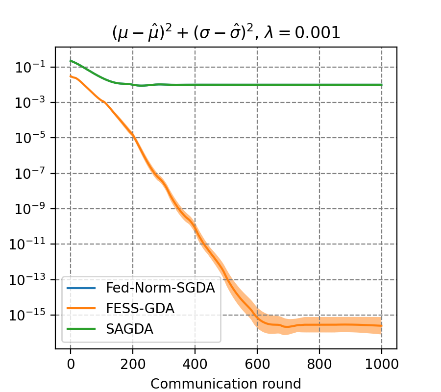
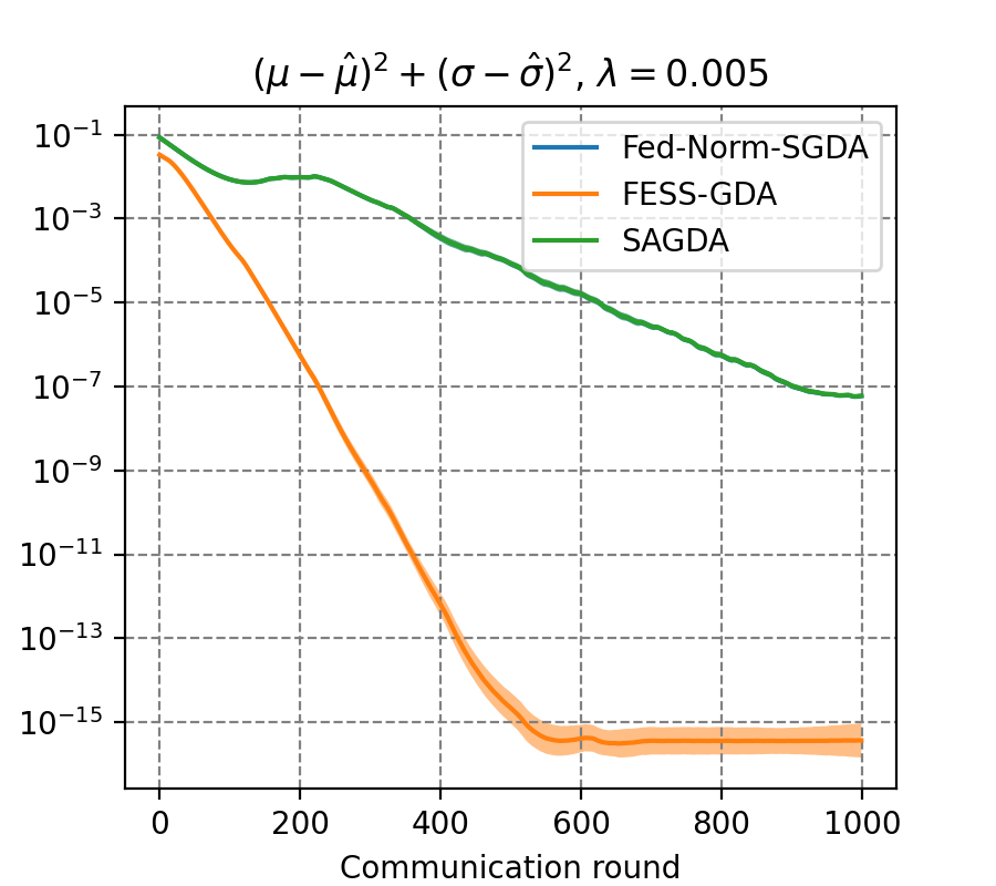
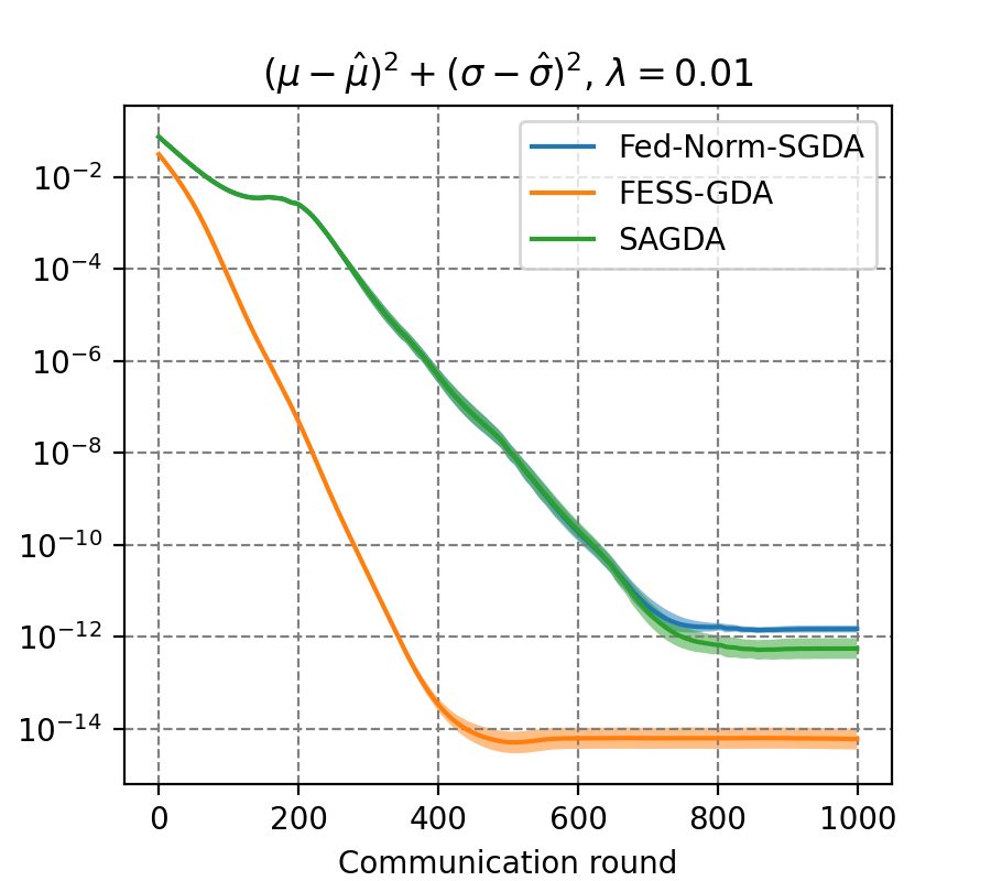
Figure 1: Comparison between Fed-Norm-SGDA and FESS-GDA for training a regularized WGAN with different regularization coefficients $\lambda$.

We perform GANs training and fair classification tasks in the federated setting to demonstrate the practical efficiency of FESS-GDA and verify our theoretical claims. We conduct our experiments in a computer with two NVIDIA RTX 3090 GPUs.

4.1 GAN

We consider a setting similar to Yang et al. (2022b), Loizou et al. (2020), using a Wasserstein GAN (Arjovsky et al., 2017) to approximate a one-dimensional Gaussian distribution in the federated setting. We first randomly generate a synthetic dataset of $n=10000$ datapoints $z$ sampled from a normal distribution with zero mean and unit variance and their corresponding real data $x^{\text{real}}=\hat{\mu}+\hat{\sigma}z$, where $\hat{\mu}=0,\hat{\sigma}=0.1$. We then evenly divide them into 10 disjoint sets for 10 clients. The generator is defined as $G_{\mu,\sigma}(z)=\mu+\sigma z$ and the discriminator is defined as $D_{\phi_{1},\phi_{2}}(x)=\phi_{1}x+\phi_{2}x^{2}$. The problem can be formulated as

$$\min_{\mu,\sigma}\max_{\phi_{1},\phi_{2}}\{f(\mu,\sigma,\phi_{1},\phi_{2})=\frac{1}{n}\sum_{j=1}^{n}D_{\phi}(x^{\text{real}}_{j})-$$

$$D_{\phi}(G_{\mu,\sigma}(z_{j}))-\lambda\|\phi\|^{2}\},$$

where $\lambda>0$ is the regularization coefficient to make the problem strongly concave.

We set a batch size of 100 for every update, and each client communicates with the server after every 10 local updates. We use the term $(\mu-\hat{\mu})^{2}+(\sigma-\hat{\sigma})^{2}$ to measure the algorithm performances.

With $\lambda=0.001,0.005,0.01$, we compare the performances between Fed-Norm-SGDA, SAGDA and FESS-GDA (see Figure 1). We use $\beta=0.05,p=1$ for FESS-GDA. For each algorithm, we test their local learning rate from $\{1e-1,1e-2,1e-3\}$ and global learning rate from $\{1,2\}$ in order to select the best for each algorithm under different $\lambda$. Each experiment is repeated 5 times and we report the average performance. As we can see from Figure 1, FESS-GDA achieves a significant speedup over Fed-Norm-SGDA and SAGDA with carefully tuned learning rates under different $\lambda$. Especially, when $\lambda$ is relatively small, the performance gap between Fed-Norm-SGDA, SAGDA and FESS-GDA is more pronounced. Note that a smaller $\lambda$ means a larger condition number $\kappa$ (if we assume that the problem has a similar Lipschitz smooth constant $l$ for different $\lambda$). This clearly validates our theoretical results that FESS-GDA improves the dependence of $\kappa$ for nonconvex-strongly-concave problems.

4.2 Fair Classification

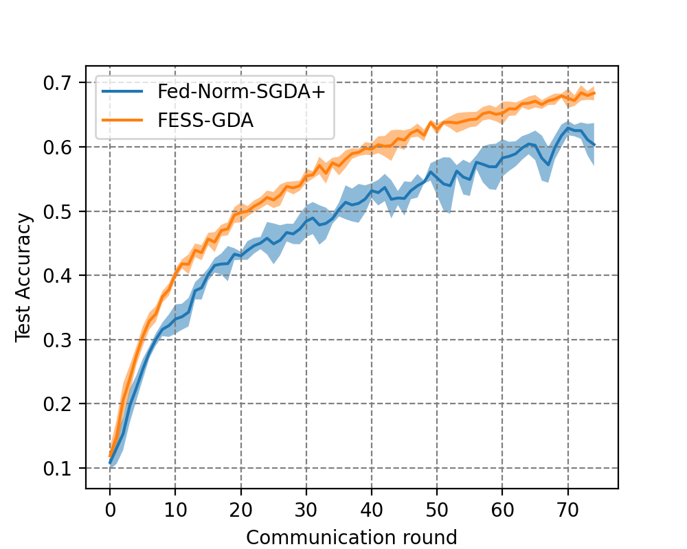
Figure 2: Comparison between Fed-Norm-SGDA+ and FESS-GDA for the fair classification task on CIFAR-10.

We consider a similar setting as Wu et al. (2023); Sharma et al. (2022); Nouiehed et al. (2019). The fair classification problem can be formulated as

$$\min_{x}\max_{y\in Y}\sum_{c=1}^{C}F_{c}(x)y_{c}$$

where $Y=\{(y_{1},...,y_{C})^{T}|\sum_{c=1}^{C},y_{c}=1,y_{c}\geq 0\}$, $x$ is the parameters of the model, and $F_{c}$ is the loss function of class $c$. Clearly, this problem has a form of (2) and is nonconvex-concave. We run the experiment on the CIFAR-10 dataset (Krizhevsky et al., 2009) with a convolutional neural network. We evenly divide the dataset into 10 disjoint sets for 10 clients. We compare the performance of Fed-Norm-SGDA+ and FESS-GDA for solving this problem and use the test accuracy as the performance measurement. We set a batch size of 100, inner loop $K=20$ for both algorithms. For both algorithms we adjust their local learning rate from $\{1e-1,1e-2\}$ and global learning rate from $\{1,1.5\}$. For FESS-GDA, we adjust its $\beta$ from $\{0.1,0.5,0.9\}$ and its $p$ from $\{0,1e-2,1e-1\}$. For Fed-Norm-SGDA+, we adjust its $S$ from $\{1,5,10,20\}$. We tune all the parameters to the best for both algorithms. Each experiment is repeated 5 times and we report the average performance. As we can see from Figure 2, FESS-GDA achieves a better performance than Fed-Norm-SGDA+.

5 Conclusion

In this paper, we have proposed a new federated minimax optimization algorithm named FESS-GDA. We showed that FESS-GDA can be uniformly used for solving different classes of federated nonconvex minimax problems and theoretically established new or better convergence results for the considered settings. We further showcased the practical efficiency of FESS-GDA in practical federated learning tasks of training GANs and fair classification tasks.

Appendix

The Appendix is organized as follows. In Section A, we introduce notations that will be used throughout the proofs. In Section B, we present some preliminary lemmas. In Section C, we derive necessary lemmas of the potential function for NC-PL and NC-1PC. In the subsequent sections, we provide the convergence results of FESS-GDA for NC-PL functions (Section D), NC-SC functions (Section E), NC-1PC functions (Section F), NC-C functions (Section G), functions having a form of (2) (Section H) and PL-PL functions (Section I). In Section J, we prove Proposition 3.1. Finally, in Section K, we provide additional results and details of our experiments.

Appendix A Notations

We introduce the following notations, which will play a significant role in our proof.

$$\hat{f}(x,y,z)=f(x,y)+\frac{p}{2}\|x-z\|^{2},$$

$$\Psi(y,z)=\min_{x\in X}\hat{f}(x,y,z),$$

$$\Phi(x)=\max_{y\in Y}f(x,y),$$

$$\Phi(x,z)=\max_{y\in Y}\hat{f}(x,y,z),,$$

$$P(z)=\min_{x\in X}\max_{y\in Y}\hat{f}(x,y,z),$$

$$V_{t}=V(x_{t},y_{t},z_{t})=\hat{f}(x_{t},y_{t},z_{t})-2\Psi(y_{t},z_{t})+2P(z_{t}),$$

$$x^{*}(y,z)=\arg\min_{x\in X}\hat{f}(x,y,z),$$

$$x^{*}(z)=\arg\min_{x\in X}\Phi(x,z),$$

$$y^{*}(x)\in\mathop{\rm argmax}_{y\in Y}f(x,y),$$

$$\hat{y}^{*}(z)\in\mathop{\rm argmax}_{y\in Y}\Psi(y,z),$$

$$x^{+}(y,z)=x-\eta_{x}K\nabla_{x}\hat{f}(x,y,z),$$

$$y^{+}(z)=P_{Y}(y+\eta_{y}K\nabla_{y}f(x^{*}(y,z),y)).$$

We denote $w_{t}=(x_{t},y_{t})$, $\eta_{x}=\eta_{x,g}\eta_{x,l}$, $\eta_{y}=\eta_{y,g}\eta_{y,l}$ for simplicity.

We summarize the main updates of FESS-GDA as:

$$x_{t+1}=x_{t}-\eta_{x}K[u_{x,t}-e_{x,t}+p(x_{t}-z_{t})],$$

$$y_{t+1}=P_{Y}(y_{t}+\eta_{y}K(u_{y,t}-e_{y,t})),$$

$$z_{t+1}=z_{t}+\beta(x_{t+1}-z_{t}),$$

$$u_{x,t}=\frac{1}{m}\sum_{i\in S_{t}}\nabla_{x}f_{i}(w_{t}),$$

$$u_{y,t}=\frac{1}{m}\sum_{i\in S_{t}}\nabla_{y}f_{i}(w_{t}),$$

$$e_{x,t}=\frac{1}{mK}\sum_{i\in S_{t}}\sum_{j\in[K]}\left(\nabla_{x}f_{i}(w_{t})-\nabla_{x}f_{i}(w^{j}_{t,i},\xi^{j}_{t,i})\right),$$

$$\bar{e}_{x,t}=\mathbb{E}[e_{x,t}]=\frac{1}{mK}\sum_{i\in S_{t}}\sum_{j\in[K]}\left(\nabla_{x}f_{i}(w_{t})-\nabla_{x}f_{i}(w^{j}_{t,i})\right),$$

$$e_{y,t}=\frac{1}{mK}\sum_{i\in S_{t}}\sum_{j\in[K]}\left(\nabla_{y}f_{i}(w_{t})-\nabla_{y}f_{i}(w^{j}_{t,i},\xi^{j}_{t,i})\right),$$

$$\bar{e}_{y,t}=\mathbb{E}[e_{y,t}]=\frac{1}{mK}\sum_{i\in S_{t}}\sum_{j\in[K]}\left(\nabla_{y}f_{i}(w_{t})-\nabla_{y}f_{i}(w^{j}_{t,i})\right).$$

We further define the following notations

$$d_{x,t}=\mathbb{E}\|\nabla_{x}\hat{f}(w_{t},z_{t})-u_{x,t}+e_{x,t}-p(x_{t}-z_{t})\|^{2},$$

$$d_{y,t}=\mathbb{E}\|\nabla_{y}f(w_{t})-u_{y,t}+e_{y,t}\|^{2}.$$

Define $\bar{y}_{t+1}=P_{Y}(y_{t}+\eta_{y}K\nabla_{y}f(w_{t}))$, when $Y=\mathbb{R}^{d_{2}}$, we have $\bar{y}_{t+1}=y_{t}+\eta_{y}K\nabla_{y}f(w_{t})$. Define $\Phi^{*}=\min_{x\in X}\max_{y\in Y}f(x,y),\quad\Delta=V_{0}-\Phi^{*}$. Because $V(x,y,z)=P(z)+(f(x,y,z)-\Psi(y,z))+(P(z)-\Psi(y,z))\geq P(z)\geq\Phi^{*}$, we have

$$V_{0}-V_{t}\leq V_{0}-\min V_{t}\leq V_{0}-\Phi^{*}=\Delta.$$ (4)

Appendix B Preliminary Lemmas

Lemma B.1 (Lemma C.1 [Yang et al., 2022b])

When $p>l$, we have

$$\|x^{*}(y,z)-x^{*}(y,z^{\prime})\|\leq\gamma_{1}\|z-z^{\prime}\|,$$

$$\|x^{*}(z)-x^{*}(z^{\prime})\leq\gamma_{1}\|z-z^{\prime}\|,$$

$$\|x^{*}(y,z)-x^{*}(y^{\prime},z)\|\leq\gamma_{2}\|y-y^{\prime}\|,$$

where $\gamma_{1}=\frac{p}{-l+p}$, $\gamma_{2}=\frac{l+p}{-l+p}$.

Lemma B.2 (Karimi et al. [2016])

If function $g(x)$ is $l$-smooth and satisfies PL condition with constant $\mu$, then the following conditions hold

$$g(x)-\min_{z}g(z) \geq\frac{\mu}{2}\|x_{p}-x\|^{2},$$

$$\|\nabla_{x}g(x)\|^{2} \geq 2\mu(g(x)-\min_{z}g(z)),$$

$$\|\nabla_{x}g(x)\|^{2} \geq\mu\|x_{p}-x\|^{2},$$

where $x_{p}$ is the projection of $x$ onto the optimal set.

Lemma B.3

When $p=2l$, we have

$$\|\nabla_{x}\Phi(x^{*}(x_{t}))\|=\|\nabla_{x}\Phi_{1/2l}(x_{t})\|=p\|x_{t}-x^{*}(x_{t})\|.$$

Proof   Note that $x^{*}(x_{t})=\mathop{\rm argmin}_{x}\{\max_{y}f(x,y)+\frac{p}{2}\|x-x_{t}\|^{2}\}$. According to Lemma A.4 in Yang et al. [2022b], we have $\|\nabla_{x}\Phi(x^{*}(x_{t}))\|=\|\nabla_{x}\Phi_{1/2l}(x_{t})\|=p\|x_{t}-x^{*}(x_{t})\|$. $\blacksquare$

Lemma B.4

When the local step sizes $\eta_{x,l},\eta_{y,l}$ satisfy

$$\eta_{x,l}\leq \frac{1}{2l\sqrt{2(2K-1)(K-1)}},$$

$$\eta_{y,l}\leq \frac{1}{2l\sqrt{2(2K-1)(K-1)}},$$

the following two inequalities hold:

$$\mathbb{E}\|\bar{e}_{x,t}\|^{2}\leq l^{2}[24K^{2}\eta_{x,l}^{2}\mathbb{E}\|\nabla_{x}f(w_{t})\|^{2}+24K^{2}\eta_{y,l}^{2}\mathbb{E}\|\nabla_{y}f(w_{t})\|^{2}+24K^{2}(\eta_{x,l}^{2}+\eta_{y,l}^{2})\sigma_{G}^{2}+3K(\eta_{x,l}^{2}+2K\eta_{y,l}^{2})\sigma^{2}],$$

$$\mathbb{E}\|\bar{e}_{y,t}\|^{2}\leq l^{2}[24K^{2}\eta_{x,l}^{2}\mathbb{E}\|\nabla_{x}f(w_{t})\|^{2}+24K^{2}\eta_{y,l}^{2}\mathbb{E}\|\nabla_{y}f(w_{t})\|^{2}+24K^{2}(\eta_{x,l}^{2}+\eta_{y,l}^{2})\sigma_{G}^{2}+3K(\eta_{x,l}^{2}+2K\eta_{y,l}^{2})\sigma^{2}].$$

Proof   According to the definition of $\|\bar{e}_{x,t}\|$, we have

$$\mathbb{E}\|w_{t}-w_{t,i}^{j+1}\|^{2}$$

$$= \mathbb{E}\|x^{j}_{t,i}-\eta_{x,l}\nabla_{x}f_{i}(w^{j}_{t,i},\xi^{j}_{t,i})-x_{t}\|^{2}+\mathbb{E}\|P_{Y}(y^{j}_{t,i}+\eta_{y,l}\nabla_{y}f_{i}(w^{j}_{t,i},\xi^{j}_{t,i}))-y_{t}\|^{2}$$

$$\overset{(a)}{\leq} \mathbb{E}\|x^{j}_{t,i}-x_{t}-\eta_{x,l}\nabla_{x}f_{i}(w^{j}_{t,i})\|^{2}+\mathbb{E}\|P_{Y}(y^{j}_{t,i}+\eta_{y,l}\nabla_{y}f_{i}(w^{j}_{t,i},\xi^{j}_{t,i}))-y_{t}\|^{2}+\eta_{x,l}^{2}\sigma^{2}$$

$$\overset{(b)}{\leq} \left(1+\frac{1}{2K-1}\right)\mathbb{E}\|x_{t,i}^{j}-x_{t}\|^{2}+2K\eta_{x,l}^{2}\|\nabla_{x}f_{i}(w_{t,i}^{j})\|^{2}+\left(1+\frac{1}{2K-1}\right)\mathbb{E}\|y_{t,i}^{j}-y_{t}\|^{2}+$$

$$2K\mathbb{E}\|P_{Y}(y_{t,i}^{j}+\eta_{y,l}\nabla_{y}f_{i}(w_{t,i}^{j},\xi^{j}_{t,i}))-y_{t,i}^{j}\|^{2}+\eta_{x,l}^{2}\sigma^{2}$$

$$\overset{(c)}{\leq} \left(1+\frac{1}{2K-1}\right)\mathbb{E}\|w_{t,i}^{j}-w_{t}\|^{2}+2K\eta_{x,l}^{2}\mathbb{E}\|\nabla_{x}f_{i}(w_{t,i}^{j})\|^{2}+2K\eta_{y,l}^{2}\mathbb{E}\|\nabla_{y}f_{i}(w_{t,i}^{j},\xi^{j}_{t,i})\|^{2}+\eta_{x,l}^{2}\sigma^{2}$$

$$\overset{(d)}{\leq} \left(1+\frac{1}{2K-1}\right)\mathbb{E}\|w_{t,i}^{j}-w_{t}\|^{2}+2K\eta_{x,l}^{2}\mathbb{E}\|\nabla_{x}f_{i}(w_{t,i}^{j})\|^{2}+2K\eta_{y,l}^{2}\mathbb{E}\|\nabla_{y}f_{i}(w_{t,i}^{j})\|^{2}+(\eta_{x,l}^{2}+2K\eta_{y,l}^{2})\sigma^{2}$$

$$\leq \left(1+\frac{1}{2K-1}\right)\mathbb{E}\|w_{t,i}^{j}-w_{t}\|^{2}+4K\eta_{x,l}^{2}\mathbb{E}\|\nabla_{x}f_{i}(w_{t})\|^{2}+4K\eta_{y,l}^{2}\mathbb{E}\|\nabla_{y}f_{i}(w_{t})\|^{2}+(\eta_{x,l}^{2}+2K\eta_{y,l}^{2})\sigma^{2}+$$

$$4K\eta_{x,l}^{2}\mathbb{E}\|\nabla_{x}f_{i}(w_{t})-\nabla_{x}f_{i}(w_{t,i}^{j})\|^{2}+4K\eta_{y,l}^{2}\mathbb{E}\|\nabla_{y}f_{i}(w_{t})-\nabla_{y}f_{i}(w_{t,i}^{j})\|^{2}$$

$$\overset{(e)}{\leq} \left(1+\frac{1}{2K-1}\right)\mathbb{E}\|w_{t,i}^{j}-w_{t}\|^{2}+4K\eta_{x,l}^{2}\mathbb{E}\|\nabla_{x}f_{i}(w_{t})\|^{2}+4K\eta_{y,l}^{2}\mathbb{E}\|\nabla_{y}f_{i}(w_{t})\|^{2}+(\eta_{x,l}^{2}+2K\eta_{y,l}^{2})\sigma^{2}+$$

$$4K\eta_{x,l}^{2}l^{2}\|w_{t}-w_{t,i}^{j}\|^{2}+4K\eta_{y,l}^{2}l^{2}\|w_{t}-w_{t,i}^{j}\|^{2}$$

$$= \left(1+\frac{1}{2K-1}+4Kl^{2}(\eta_{x,l}^{2}+\eta_{y,l}^{2})\right)\mathbb{E}\|w_{t,i}^{j}-w_{t}\|^{2}+4K\eta_{x,l}^{2}\mathbb{E}\|\nabla_{x}f_{i}(w_{t})\|^{2}+4K\eta_{y,l}^{2}\mathbb{E}\|\nabla_{y}f_{i}(w_{t})\|^{2}+$$

$$(\eta_{x,l}^{2}+2K\eta_{y,l}^{2})\sigma^{2}$$

$$\overset{(f)}{\leq} \left(1+\frac{1}{K-1}\right)\mathbb{E}\|w_{t,i}^{j}-w_{t}\|^{2}+4K\eta_{x,l}^{2}\mathbb{E}\|\nabla_{x}f_{i}(w_{t})\|^{2}+4K\eta_{y,l}^{2}\mathbb{E}\|\nabla_{y}f_{i}(w_{t})\|^{2}+(\eta_{x,l}^{2}+2K\eta_{y,l}^{2})\sigma^{2}$$

$$\overset{(g)}{\leq} \sum_{\tau=0}^{j-1}\left(1+\frac{1}{K-1}\right)^{\tau}[4K\eta_{x,l}^{2}\mathbb{E}\|\nabla_{x}f_{i}(w_{t})\|^{2}+4K\eta_{y,l}^{2}\mathbb{E}\|\nabla_{y}f_{i}(w_{t})\|^{2}+(\eta_{x,l}^{2}+2K\eta_{y,l}^{2})\sigma^{2}]$$

$$\overset{(h)}{\leq} 12K^{2}\eta_{x,l}^{2}\mathbb{E}\|\nabla_{x}f_{i}(w_{t})\|^{2}+12K^{2}\eta_{y,l}^{2}\mathbb{E}\|\nabla_{y}f_{i}(w_{t})\|^{2}+3K(\eta_{x,l}^{2}+2K\eta_{y,l}^{2})\sigma^{2}$$

$$\overset{(i)}{\leq} 24K^{2}\eta_{x,l}^{2}\mathbb{E}\|\nabla_{x}f(w_{t})\|^{2}+24K^{2}\eta_{y,l}^{2}\mathbb{E}\|\nabla_{y}f(w_{t})\|^{2}+24K^{2}(\eta_{x,l}^{2}+\eta_{y,l}^{2})\sigma_{G}^{2}+3K(\eta_{x,l}^{2}+2K\eta_{y,l}^{2})\sigma^{2}.$$

The $(a),(d)$ are a consequence of the bounded variance of the stochastic gradient. $(b)$ arises from the property that $\|a+b\|^{2}\leq(1+c)\|a\|^{2}+(1+1/c)\|b\|^{2},c>0$. $(c)$ is a result of the nonexpansiveness of the projection operator. $(e)$ is derived from the $l$-smoothness of the function $f$, while $(f)$ is established based on the condition:

$$l^{2}\eta_{x,l}^{2}\leq \frac{1}{8(2K-1)(K-1)},$$

$$l^{2}\eta_{y,l}^{2}\leq \frac{1}{8(2K-1)(K-1)}.$$

$(h)$ is due to

$$\sum_{\tau=0}^{j-1}\left(1+\frac{1}{K-1}\right)^{\tau}\leq (K-1)\left(\frac{K}{K-1}\right)^{K}$$

$$\frac{1}{K}\sum_{\tau=0}^{j-1}\left(1+\frac{1}{K-1}\right)^{\tau}\leq \left(\frac{K}{K-1}\right)^{K-1}\leq e\leq 3$$

$$\sum_{\tau=0}^{j-1}\left(1+\frac{1}{K-1}\right)^{\tau}\leq 3K.$$

$(i)$ is from Assumption 2.3. We thus have

$$\mathbb{E}\|\bar{e}_{x,t}\|^{2}\leq l^{2}[24K^{2}\eta_{x,l}^{2}\mathbb{E}\|\nabla_{x}f(w_{t})\|^{2}+24K^{2}\eta_{y,l}^{2}\mathbb{E}\|\nabla_{y}f(w_{t})\|^{2}+24K^{2}(\eta_{x,l}^{2}+\eta_{y,l}^{2})\sigma_{G}^{2}+3K(\eta_{x,l}^{2}+2K\eta_{y,l}^{2})\sigma^{2}].$$

The inequality for $y$ can be proven in a similar fashion. $\blacksquare$

Lemma B.5

The following inequalities establish upper bounds for $d_{x,t}$ and $d_{y,t}$:

$$d_{x,t}= \mathbb{E}\|\nabla_{x}\hat{f}(w_{t},z_{t})-u_{x,t}+e_{x,t}-p(x_{t}-z_{t})\|^{2}\leq 2\mathbb{E}\|\bar{e}_{x,t}\|^{2}+4\left(M-m\right)\frac{\sigma_{G}^{2}}{mM}+\frac{2}{mK}\sigma^{2},$$

$$d_{y,t}= \mathbb{E}\|\nabla_{y}f(w_{t})-u_{y,t}+e_{y,t}\|^{2}\leq 2\mathbb{E}\|\bar{e}_{y,t}\|^{2}+4\left(M-m\right)\frac{\sigma_{G}^{2}}{mM}+\frac{2}{mK}\sigma^{2}.$$

Proof   According to the definition of $d_{x,t}$, we have

$$d_{x,t}= \mathbb{E}\|\nabla_{x}\hat{f}(w_{t},z_{t})-u_{x,t}+e_{x,t}-p(x_{t}-z_{t})\|^{2}$$

$$= \mathbb{E}\|\nabla_{x}f(w_{t})-u_{x,t}+e_{x,t}\|^{2}$$

$$\leq 2\mathbb{E}\|\nabla_{x}f(w_{t})-u_{x,t}\|^{2}+2\mathbb{E}\|e_{x,t}\|^{2}$$

$$\leq 2\mathbb{E}\left\|\frac{1}{M}\sum_{j\in[M]}\nabla_{x}f_{j}(w_{t})-\frac{1}{m}\sum_{i\in S_{t}}\nabla_{x}f_{i}(w_{t})\right\|^{2}+2\mathbb{E}\|\bar{e}_{x,t}\|^{2}+\frac{2}{mK}\sigma^{2}$$

$$\leq 2\mathbb{E}\left\|\left(\frac{1}{M}-\frac{1}{m}\right)\sum_{j\in S_{t}}\nabla_{x}f_{j}(w_{t})-m\left(\frac{1}{M}-\frac{1}{m}\right)\nabla_{x}f(w_{t})+\frac{1}{M}\sum_{i\in[M]/S_{t}}\nabla_{x}f_{i}(w_{t})-\frac{M-m}{M}\nabla_{x}f(w_{t})\right\|^{2}+$$

$$2\mathbb{E}\|\bar{e}_{x,t}\|^{2}+\frac{2}{mK}\sigma^{2}$$

$$\leq 4\mathbb{E}\left\|\left(\frac{1}{M}-\frac{1}{m}\right)\sum_{j\in S_{t}}\nabla_{x}f_{j}(w_{t})-m\left(\frac{1}{M}-\frac{1}{m}\right)\nabla_{x}f(w_{t})\right\|^{2}+$$

$$4\mathbb{E}\left\|\frac{1}{M}\sum_{i\in[M]/S_{t}}\nabla_{x}f_{i}(w_{t})-\frac{M-m}{M}\nabla_{x}f(w_{t})\right\|^{2}+2\mathbb{E}\|\bar{e}_{x,t}\|^{2}+\frac{2}{mK}\sigma^{2}$$

$$\overset{(a)}{\leq} 4\left[m\left(\frac{1}{M}-\frac{1}{m}\right)^{2}+(M-m)\frac{1}{M^{2}}\right]\sigma_{G}^{2}+2\mathbb{E}\|\bar{e}_{x,t}\|^{2}+\frac{2}{mK}\sigma^{2}$$

$$\leq 2\mathbb{E}\|\bar{e}_{x,t}\|^{2}+4\left(M-m\right)\frac{\sigma_{G}^{2}}{mM}+\frac{2}{mK}\sigma^{2},$$

where $(a)$ is due to $\|\sum_{i}^{k}x_{i}\|^{2}\leq k\sum_{i}^{k}\|x_{i}\|^{2}$ and Assumption 2.3. Similarly, we have

$$d_{y,t}= \mathbb{E}\|\nabla_{y}f(w_{t})-u_{y,t}+e_{y,t}\|^{2}\leq 2\mathbb{E}\|\bar{e}_{y,t}\|^{2}+4\left(M-m\right)\frac{\sigma_{G}^{2}}{mM}+\frac{2}{mK}\sigma^{2}.$$

$\blacksquare$

Lemma B.6

Under the update rule of FESS-GDA, we have

$$\mathbb{E}\|x_{t+1}-x_{t}\|^{2}\leq 2\eta_{x}^{2}K^{2}\mathbb{E}\|\nabla_{x}\hat{f}(w_{t},z_{t})\|^{2}+2\eta_{x}^{2}K^{2}d_{x,t},$$

$$\mathbb{E}\|y_{t+1}-y_{t}\|^{2}\leq 2\mathbb{E}\|\bar{y}_{t+1}-y_{t}\|^{2}+2\eta_{y}^{2}K^{2}d_{y,t}.$$

When $Y=\mathbb{R}^{d_{2}}$, we have $\mathbb{E}\|y_{t+1}-y_{t}\|^{2}\leq 2\eta_{y}^{2}K^{2}\mathbb{E}\|\nabla_{y}f(w_{t})\|^{2}+2\eta_{y}^{2}K^{2}d_{y,t}$.

Proof   According to the update rule of $x_{t},y_{t}$, we have

$$\mathbb{E}\|x_{t+1}-x_{t}\|^{2}= \eta_{x}^{2}K^{2}\mathbb{E}\|u_{x,t}-e_{x,t}-p(x_{t}-z_{t})\|^{2}$$

$$\leq 2\eta_{x}^{2}K^{2}\mathbb{E}\|\nabla_{x}\hat{f}(w_{t},z_{t})\|^{2}+2\eta_{x}^{2}K^{2}\mathbb{E}\|\nabla_{x}\hat{f}(w_{t},z_{t})-u_{x,t}+e_{x,t}-p(x_{t}-z_{t})\|^{2}$$

$$= 2\eta_{x}^{2}K^{2}\mathbb{E}\|\nabla_{x}\hat{f}(w_{t},z_{t})\|^{2}+2\eta_{x}^{2}K^{2}d_{x,t},$$

$$\mathbb{E}\|y_{t+1}-y_{t}\|^{2}= \mathbb{E}\|P_{Y}(y_{t}+\eta_{y}K(u_{y,t}-e_{y,t}))-y_{t}\|^{2}$$

$$\overset{(a)}{\leq} 2\mathbb{E}\|P_{Y}(y_{t}+\eta_{y}K\nabla_{y}f(w_{t}))-y_{t}\|^{2}+2\eta_{y}^{2}K^{2}\|\nabla_{y}f(w_{t})-u_{y,t}+e_{y,t}\|^{2}$$

$$= 2\mathbb{E}\|\bar{y}_{t+1}-y_{t}\|^{2}+2\eta_{y}^{2}K^{2}d_{y,t},$$

where $(a)$ is due to the nonexpansiveness of the projection operator. $\blacksquare$

Appendix C Intermediate Lemmas for Potential Function

Recall the potential function is defined as

$$V_{t}=V(x_{t},y_{t},z_{t})=\hat{f}(x_{t},y_{t},z_{t})-2\Psi(y_{t},z_{t})+2P(z_{t}).$$

The outline of the convergence proof for FESS-GDA aims to demonstrate the monotonic decrease of $V_{t}$. In this section, we present the essential lemmas required to establish bounds on the potential function.

Lemma C.1

When $\eta_{x}\leq\frac{1}{4(p+l)K}$, we have the following inequality:

$$\mathbb{E}\hat{f}(w_{t},z_{t})-\mathbb{E}\hat{f}(w_{t+1},z_{t})$$

$$\geq \frac{\eta_{x}K}{4}\|\nabla_{x}\hat{f}(w_{t},z_{t})\|^{2}-\frac{\eta_{x}K}{2}\|\bar{e}_{x,t}\|^{2}-(p+l)\eta_{x}^{2}K^{2}d_{x,t}+\mathbb{E}\langle\nabla_{y}f(w_{t}),y_{t}-y_{t+1}\rangle-\frac{p+l}{2}\mathbb{E}\|y_{t+1}-y_{t}\|^{2}.$$

Proof   Because of the $(p+l)$-smoothness of $\hat{f}(\cdot,z)$, we have

$$\mathbb{E}\hat{f}(w_{t},z_{t})-\mathbb{E}\hat{f}(w_{t+1},z_{t})$$

$$\geq \mathbb{E}\langle\nabla_{x}\hat{f}(w_{t},z_{t}),x_{t}-x_{t+1}\rangle+\mathbb{E}\langle\nabla_{y}\hat{f}(w_{t},z_{t}),y_{t}-y_{t+1}\rangle-\frac{p+l}{2}\mathbb{E}\|x_{t+1}-x_{t}\|^{2}-\frac{p+l}{2}\mathbb{E}\|y_{t+1}-y_{t}\|^{2}$$

$$= \eta_{x}K\mathbb{E}\langle\nabla_{x}\hat{f}(w_{t},z_{t}),u_{x,t}+p(x_{t}-z_{t})-\bar{e}_{x,t}\rangle+\mathbb{E}\langle\nabla_{y}f(w_{t}),y_{t}-y_{t+1}\rangle-\frac{p+l}{2}\mathbb{E}\|x_{t+1}-x_{t}\|^{2}-\frac{p+l}{2}\mathbb{E}\|y_{t+1}-y_{t}\|^{2}$$

$$= \eta_{x}K\mathbb{E}\langle\nabla_{x}\hat{f}(w_{t},z_{t}),\nabla_{x}\hat{f}(w_{t},z_{t})-\bar{e}_{x,t}\rangle+\mathbb{E}\langle\nabla_{y}f(w_{t}),y_{t}-y_{t+1}\rangle-\frac{p+l}{2}\mathbb{E}\|x_{t+1}-x_{t}\|^{2}-\frac{p+l}{2}\mathbb{E}\|y_{t+1}-y_{t}\|^{2}$$

$$= \eta_{x}K\mathbb{E}\|\nabla_{x}\hat{f}(w_{t},z_{t})\|^{2}+\frac{\eta_{x}K}{2}\mathbb{E}\|\nabla_{x}\hat{f}(w_{t},z_{t})-\bar{e}_{x,t}\|^{2}-\frac{\eta_{x}K}{2}\mathbb{E}\|\nabla_{x}\hat{f}(w_{t},z_{t})\|^{2}-\frac{\eta_{x}K}{2}\mathbb{E}\|\bar{e}_{x,t}\|^{2}+$$

$$\mathbb{E}\langle\nabla_{y}f(w_{t}),y_{t}-y_{t+1}\rangle-\frac{p+l}{2}\mathbb{E}\|x_{t+1}-x_{t}\|^{2}-\frac{p+l}{2}\mathbb{E}\|y_{t+1}-y_{t}\|^{2}$$

$$\geq \frac{\eta_{x}K}{2}\mathbb{E}\|\nabla_{x}\hat{f}(w_{t},z_{t})\|^{2}-\frac{\eta_{x}K}{2}\mathbb{E}\|\bar{e}_{x,t}\|^{2}+\mathbb{E}\langle\nabla_{y}f(w_{t}),y_{t}-y_{t+1}\rangle-\frac{p+l}{2}\mathbb{E}\|x_{t+1}-x_{t}\|^{2}-\frac{p+l}{2}\mathbb{E}\|y_{t+1}-y_{t}\|^{2}$$

$$\overset{(a)}{\geq} (\frac{\eta_{x}K}{2}-(p+l)\eta_{x}^{2}K^{2})\mathbb{E}\|\nabla_{x}\hat{f}(w_{t},z_{t})\|^{2}-(p+l)\eta_{x}^{2}K^{2}d_{x,t}-\frac{\eta_{x}K}{2}\mathbb{E}\|\bar{e}_{x,t}\|^{2}+$$

$$\mathbb{E}\langle\nabla_{y}f(w_{t}),y_{t}-y_{t+1}\rangle-\frac{p+l}{2}\mathbb{E}\|y_{t+1}-y_{t}\|^{2}$$

$$\overset{(b)}{\geq} \frac{\eta_{x}K}{4}\mathbb{E}\|\nabla_{x}\hat{f}(w_{t},z_{t})\|^{2}-\frac{\eta_{x}K}{2}\mathbb{E}\|\bar{e}_{x,t}\|^{2}-(p+l)\eta_{x}^{2}K^{2}d_{x,t}+\mathbb{E}\langle\nabla_{y}f(w_{t}),y_{t}-y_{t+1}\rangle-\frac{p+l}{2}\mathbb{E}\|y_{t+1}-y_{t}\|^{2}$$

where the $(a)$ is due to the Lemma B.6, and $(b)$ is due to the condition $\eta_{x}\leq\frac{1}{4(p+l)K}$. $\blacksquare$

Lemma C.2

The $z$-update in FESS-GDA yields

$$\hat{f}(w_{t+1},z_{t})-\hat{f}(w_{t+1},z_{t+1})\geq \frac{p}{2\beta}\|z_{t}-z_{t+1}\|^{2}.$$

Proof   By definition of $\hat{f}$ and the update rule of $z$, as $0<\beta<1$, we have

$$\hat{f}(w_{t+1},z_{t})-\hat{f}(w_{t+1},z_{t+1})= \frac{p}{2}[\|x_{t+1}-z_{t}\|^{2}-\|x_{t+1}-z_{t+1}\|^{2}]$$

$$= \frac{p}{2}\left[\frac{1}{\beta^{2}}\|(z_{t+1}-z_{t})\|^{2}-\|(1-\beta)(x_{t+1}-z_{t})\|^{2}\right]$$

$$= \frac{p}{2}\left[\frac{1}{\beta^{2}}\|z_{t+1}-z_{t}\|^{2}-\frac{(1-\beta)^{2}}{\beta^{2}}\|z_{t+1}-z_{t}\|^{2}\right]$$

$$\geq \frac{p}{2\beta}\|z_{t}-z_{t+1}\|^{2}.$$

$\blacksquare$

Lemma C.3

With $L_{\Psi}=l+l\gamma_{2}$, $\gamma_{2}=\frac{l+p}{p-l}$, we have

$$\Psi(y_{t+1},z_{t})-\Psi(y_{t},z_{t})\geq \langle\nabla_{y}\Psi(y_{t},z_{t}),y_{t+1}-y_{t}\rangle-\frac{L_{\Psi}}{2}\|y_{t+1}-y_{t}\|^{2},$$

$$\Psi(y_{t+1},z_{t+1})-\Psi(y_{t+1},z_{t})\geq \frac{p}{2}(z_{t+1}-z_{t})^{\top}[z_{t+1}+z_{t}-2x^{*}(y_{t+1},z_{t+1})].$$

Proof   Since the dual function $\Psi(\cdot,z)$ is $L_{\Psi}$-smooth by Lemma B.3 in Zhang et al. [2020], we have

$$\Psi(y_{t+1},z_{t})-\Psi(y_{t},z_{t})\geq \langle\nabla_{y}\Psi(y_{t},z_{t}),y_{t+1}-y_{t}\rangle-\frac{L_{\Psi}}{2}\|y_{t+1}-y_{t}\|^{2}.$$

By the definition of $x^{*}(y_{t+1},z_{t})$, we have

$$\Psi(y_{t+1},z_{t+1})-\Psi(y_{t+1},z_{t})= \hat{f}(x^{*}(y_{t+1},z_{t+1}),y_{t+1},z_{t+1})-\hat{f}(x^{*}(y_{t+1},z_{t}),y_{t+1},z_{t})$$

$$\geq \hat{f}(x^{*}(y_{t+1},z_{t+1}),y_{t+1},z_{t+1})-\hat{f}(x^{*}(y_{t+1},z_{t+1}),y_{t+1},z_{t})$$

$$= \frac{p}{2}\left[\|z_{t+1}-x^{*}(y_{t+1},z_{t+1})\|^{2}-\|z_{t}-x^{*}(y_{t+1},z_{t+1})\|^{2}\right]$$

$$= \frac{p}{2}(z_{t+1}-z_{t})^{\top}[z_{t+1}+z_{t}-2x^{*}(y_{t+1},z_{t+1})].$$

$\blacksquare$

Lemma C.4

$$P(z_{t+1})-P(z_{t})\leq \frac{p}{2}(z_{t+1}-z_{t})^{\top}[z_{t+1}+z_{t}-2x^{*}(\hat{y}^{*}(z_{t+1}),z_{t})].$$

Proof   By the definition of $\hat{y}^{*}(z_{t})$ and $x^{*}(\hat{y}^{*}(z_{t+1}),z_{t+1})$, we have

$$P(z_{t+1})-P(z_{t})= \Psi(\hat{y}^{*}(z_{t+1}),z_{t+1})-\Psi(\hat{y}^{*}(z_{t}),z_{t})$$

$$\leq \Psi(\hat{y}^{*}(z_{t+1}),z_{t+1})-\Psi(\hat{y}^{*}(z_{t+1}),z_{t})$$

$$= \hat{f}(x^{*}(\hat{y}^{*}(z_{t+1}),z_{t+1}),\hat{y}^{*}(z_{t+1}),z_{t+1})-\hat{f}(x^{*}(\hat{y}^{*}(z_{t+1}),z_{t}),\hat{y}^{*}(z_{t+1}),z_{t})$$

$$\leq \hat{f}(x^{*}(\hat{y}^{*}(z_{t+1}),z_{t}),\hat{y}^{*}(z_{t+1}),z_{t+1})-\hat{f}(x^{*}(\hat{y}^{*}(z_{t+1}),z_{t}),\hat{y}^{*}(z_{t+1}),z_{t})$$

$$= \frac{p}{2}(z_{t+1}-z_{t})^{\top}[z_{t+1}+z_{t}-2x^{*}(\hat{y}^{*}(z_{t+1}),z_{t})].$$

$\blacksquare$

Lemma C.5

The following inequality holds:

$$2\mathbb{E}(\Psi(y_{t+1},z_{t+1})-\Psi(y_{t+1},z_{t}))-2\mathbb{E}(P(z_{t+1})-P(z_{t}))$$

$$\geq -\left(2p\gamma_{1}+\frac{p}{6\beta}-48p\beta\gamma_{1}^{2}\right)\|z_{t+1}-z_{t}\|^{2}-24p\beta\mathbb{E}\|x^{*}(z_{t})-x^{*}(y_{t},z_{t})\|^{2}-48p\beta\gamma_{2}^{2}\|\bar{y}_{t+1}-y_{t}\|^{2}-$$

$$48p\beta\gamma_{2}^{2}\eta_{y}^{2}K^{2}d_{y,t}.$$

Proof   Combining Lemmas C.3 and C.4, we have

$$2\mathbb{E}(\Psi(y_{t+1},z_{t+1})-\Psi(y_{t+1},z_{t}))-2\mathbb{E}(P(z_{t+1})-P(z_{t}))$$

$$\geq 2p\mathbb{E}(z_{t+1}-z_{t})^{\top}[x^{*}(\hat{y}^{*}(z_{t+1}),z_{t})-x^{*}(y_{t+1},z_{t+1})]$$

$$= 2p\mathbb{E}(z_{t+1}-z_{t})^{\top}[x^{*}(\hat{y}^{*}(z_{t+1}),z_{t})-x^{*}(\hat{y}^{*}(z_{t+1}),z_{t+1})]+2p\mathbb{E}(z_{t+1}-z_{t})^{\top}[x^{*}(\hat{y}^{*}(z_{t+1}),z_{t+1})-x^{*}(y_{t+1},z_{t+1})]$$

$$\overset{(a)}{\geq} -2p\gamma_{1}\|z_{t+1}-z_{t}\|^{2}+2p\mathbb{E}(z_{t+1}-z_{t})^{\top}[x^{*}(\hat{y}^{*}(z_{t+1}),z_{t+1})-x^{*}(y_{t+1},z_{t+1})]$$

$$\geq -\left(2p\gamma_{1}+\frac{p}{6\beta}\right)\|z_{t+1}-z_{t}\|^{2}-6p\beta\mathbb{E}\|x^{*}(z_{t+1})-x^{*}(y_{t+1},z_{t+1})\|^{2}$$

$$\geq -\left(2p\gamma_{1}+\frac{p}{6\beta}\right)\|z_{t+1}-z_{t}\|^{2}-24p\beta\mathbb{E}\|x^{*}(z_{t})-x^{*}(y_{t},z_{t})\|^{2}-24p\beta\mathbb{E}\|x^{*}(z_{t})-x^{*}(z_{t+1})\|^{2}-$$

$$24p\beta\mathbb{E}\|x^{*}(y_{t+1},z_{t+1})-x^{*}(y_{t+1},z_{t})\|^{2}-24p\beta\mathbb{E}\|x^{*}(y_{t+1},z_{t})-x^{*}(y_{t},z_{t})\|^{2}$$

$$\overset{(b)}{\geq} -\left(2p\gamma_{1}+\frac{p}{6\beta}+48p\beta\gamma_{1}^{2}\right)\|z_{t+1}-z_{t}\|^{2}-24p\beta\mathbb{E}\|x^{*}(z_{t})-x^{*}(y_{t},z_{t})\|^{2}-24p\beta\gamma_{2}^{2}\|y_{t+1}-y_{t}\|^{2}$$

$$\overset{(c)}{\geq} -\left(2p\gamma_{1}+\frac{p}{6\beta}+48p\beta\gamma_{1}^{2}\right)\|z_{t+1}-z_{t}\|^{2}-24p\beta\mathbb{E}\|x^{*}(z_{t})-x^{*}(y_{t},z_{t})\|^{2}-48p\beta\gamma_{2}^{2}\|\bar{y}_{t+1}-y_{t}\|^{2}-$$

$$48p\beta\gamma_{2}^{2}\eta_{y}^{2}K^{2}d_{y,t},$$

where $(a)$ and $(b)$ are due to Lemma B.1, and $(c)$ is due to Lemma B.6. $\blacksquare$

Lemma C.6

Suppose we have $\eta_{y}\leq\frac{1}{8(2L_{\Psi}+l+p)K}$, $\eta_{y}=\eta_{x}/256$ and $p=2l$. In the unconstrained case when $Y=\mathbb{R}^{d_{2}}$, we have

$$\mathbb{E}\hat{f}(w_{t},z_{t})-\mathbb{E}\hat{f}(w_{t+1},z_{t})+2(\mathbb{E}\Psi(y_{t+1},z_{t})-\mathbb{E}\Psi(y_{t},z_{t}))$$

$$\geq \frac{\eta_{x}K}{8}\mathbb{E}\|\nabla_{x}\hat{f}(w_{t},z_{t})\|^{2}+\frac{\eta_{y}K}{8}\mathbb{E}\|\nabla_{y}f(w_{t})\|^{2}-\frac{\eta_{x}K}{2}\mathbb{E}\|\bar{e}_{x,t}\|^{2}-(p+l)\eta_{x}^{2}K^{2}d_{x,t}-$$

$$\frac{3\eta_{y}K}{4}\mathbb{E}\|\bar{e}_{y,t}\|^{2}-(2L_{\Psi}+l+p)\eta_{y}^{2}K^{2}d_{y,t}.$$

In the constrained case when $Y\subset\mathbb{R}^{d_{2}}$ is convex and compact, we have

$$\mathbb{E}\hat{f}(w_{t},z_{t})-\mathbb{E}\hat{f}(w_{t+1},z_{t})+2(\mathbb{E}\Psi(y_{t+1},z_{t})-\mathbb{E}\Psi(y_{t},z_{t}))$$

$$\geq \frac{\eta_{x}K}{8}\mathbb{E}\|\nabla_{x}\hat{f}(w_{t},z_{t})\|^{2}+\frac{1}{8\eta_{y}K}\mathbb{E}\|\bar{y}_{t+1}-y_{t}\|^{2}-\frac{\eta_{x}K}{2}\mathbb{E}\|\bar{e}_{x,t}\|^{2}-(p+l)\eta_{x}^{2}K^{2}d_{x,t}-$$

$$4\eta_{y}K\mathbb{E}\|\bar{e}_{y,t}\|^{2}-2\eta_{y}Kd_{y,t},$$

Proof   Combining Lemmas C.2 and C.3, we have

$$\mathbb{E}\hat{f}(w_{t},z_{t})-\mathbb{E}\hat{f}(w_{t+1},z_{t})+2(\mathbb{E}\Psi(y_{t+1},z_{t})-\mathbb{E}\Psi(y_{t},z_{t}))$$

$$\geq \frac{\eta_{x}K}{4}\|\nabla_{x}\hat{f}(w_{t},z_{t})\|^{2}-\frac{\eta_{x}K}{2}\mathbb{E}\|\bar{e}_{x,t}\|^{2}-(p+l)\eta_{x}^{2}K^{2}d_{x,t}+\mathbb{E}\langle\nabla_{y}f(w_{t}),y_{t}-y_{t+1}\rangle-\frac{p+l}{2}\mathbb{E}\|y_{t+1}-y_{t}\|^{2}+$$

$$2\mathbb{E}\langle\nabla_{y}\Psi(y_{t},z_{t}),y_{t+1}-y_{t}\rangle-L_{\Psi}\mathbb{E}\|y_{t+1}-y_{t}\|^{2}.$$ (5)

Denote $A_{1}=\mathbb{E}\langle\nabla_{y}f(w_{t}),y_{t}-y_{t+1}\rangle-\frac{p+l}{2}\mathbb{E}\|y_{t+1}-y_{t}\|^{2}+2\mathbb{E}\langle\nabla_{y}\Psi(y_{t},z_{t}),y_{t+1}-y_{t}\rangle-L_{\Psi}\mathbb{E}\|y_{t+1}-y_{t}\|^{2}$.

When $Y=\mathbb{R}^{d_{2}}$, we have

$$A_{1}= \mathbb{E}\langle\nabla_{y}f(w_{t}),y_{t+1}-y_{t}\rangle+2\mathbb{E}\langle\nabla_{y}\Psi(y_{t},z_{t})-\nabla_{y}f(w_{t}),y_{t+1}-y_{t}\rangle-\frac{2L_{\Psi}+l+p}{2}\mathbb{E}\|y_{t}-y_{t+1}\|^{2}$$

$$\overset{(a)}{\geq} \eta_{y}K\mathbb{E}\langle\nabla_{y}f(w_{t}),u_{y,t}-e_{y,t}\rangle-2\eta_{y}K\mathbb{E}\langle\nabla_{y}\Psi(y_{t},z_{t})-\nabla_{y}f(w_{t}),u_{y,t}-e_{y,t}\rangle-$$

$$\eta_{y}^{2}K^{2}(2L_{\Psi}+l+p)\|\nabla_{y}f(w_{t})\|^{2}-\eta_{y}^{2}K^{2}(2L_{\Psi}+l+p)d_{y,t}$$

$$\geq \eta_{y}K\mathbb{E}\langle\nabla_{y}f(w_{t}),\nabla_{y}f(w_{t})-\bar{e}_{y,t}\rangle-2\eta_{y}K\mathbb{E}\|\nabla_{y}\Psi(y_{t},z_{t})-\nabla_{y}f(w_{t})\|\|\nabla_{y}f(w_{t})-\bar{e}_{y,t}\|-$$

$$\eta_{y}^{2}K^{2}(2L_{\Psi}+l+p)\mathbb{E}\|\nabla_{y}f(w_{t})\|^{2}-\eta_{y}^{2}K^{2}(2L_{\Psi}+l+p)d_{y,t}$$

$$\geq \eta_{y}K\mathbb{E}\|\nabla_{y}f(w_{t})\|^{2}-\frac{\eta_{y}K}{2}\mathbb{E}\|\nabla_{y}f(w_{t})\|^{2}-\frac{\eta_{y}K}{2}\mathbb{E}\|\bar{e}_{y,t}\|^{2}-\frac{\eta_{y}K}{8}\mathbb{E}\|\nabla_{y}f(w_{t})-\bar{e}_{y,t}\|^{2}-$$

$$8\eta_{y}K\mathbb{E}\|\nabla_{y}\Psi(y_{t},z_{t})-\nabla_{y}f(w_{t})\|^{2}-\eta_{y}^{2}K^{2}(2L_{\Psi}+l+p)\mathbb{E}\|\nabla_{y}f(w_{t})\|^{2}-\eta_{y}^{2}K^{2}(2L_{\Psi}+l+p)d_{y,t}$$

$$\geq \frac{\eta_{y}K}{2}\mathbb{E}\|\nabla_{y}f(w_{t})\|^{2}-\frac{\eta_{y}K}{2}\mathbb{E}\|\bar{e}_{y,t}\|^{2}-\frac{\eta_{y}K}{4}\mathbb{E}\|\nabla_{y}f(w_{t})\|^{2}-\frac{\eta_{y}K}{4}\mathbb{E}\|\bar{e}_{y,t}\|^{2}-$$

$$8\eta_{y}Kl^{2}\mathbb{E}\|x^{*}(y_{t},z_{t})-x_{t}\|^{2}-\eta_{y}^{2}K^{2}(2L_{\Psi}+l+p)\mathbb{E}\|\nabla_{y}f(w_{t})\|^{2}-\eta_{y}^{2}K^{2}(2L_{\Psi}+l+p)d_{y,t}$$

$$\overset{(b)}{\geq} \left(\frac{\eta_{y}K}{4}-\eta_{y}^{2}K^{2}(2L_{\Psi}+l+p)\right)\mathbb{E}\|\nabla_{y}f(w_{t})\|^{2}-\frac{3\eta_{y}K}{4}\mathbb{E}\|\bar{e}_{y,t}\|^{2}-(2L_{\Psi}+l+p)\eta_{y}^{2}K^{2}d_{y,t}-$$

$$\frac{8\eta_{y}Kl^{2}}{(p-l)^{2}}\mathbb{E}\|\nabla_{x}\hat{f}(w_{t},z_{t})\|^{2}$$

$$\overset{(c)}{\geq} \frac{\eta_{y}K}{8}\mathbb{E}\|\nabla_{y}f(w_{t})\|^{2}-8\eta_{y}K\mathbb{E}\|\nabla_{x}\hat{f}(w_{t},z_{t})\|^{2}-\frac{3\eta_{y}K}{4}\mathbb{E}\|\bar{e}_{y,t}\|^{2}-(2L_{\Psi}+l+p)\eta_{y}^{2}K^{2}d_{y,t}$$ (6)

where $(a)$ is due to Lemma B.6 and when $Y=\mathbb{R}^{d_{2}},y_{t+1}-y_{t}=\eta_{y}K(u_{y,t}-e_{y,t})$, $(b)$ is because of the $(p-l)$-strongly convexity of $\hat{f}(\cdot,y,z)$, and $(c)$ is due to the condition $\eta_{y}\leq\frac{1}{8(2L_{\Psi}+l+p)K}$ and $p=2l$. Combining (5) and (6), we have

$$\mathbb{E}\hat{f}(w_{t},z_{t})-\mathbb{E}\hat{f}(w_{t+1},z_{t})+2(\mathbb{E}\Psi(y_{t+1},z_{t})-\mathbb{E}\Psi(y_{t},z_{t}))$$

$$\geq \left(\frac{\eta_{x}K}{4}-8\eta_{y}K\right)\mathbb{E}\|\nabla_{x}\hat{f}(w_{t},z_{t})\|^{2}-\frac{\eta_{x}K}{2}\mathbb{E}\|\bar{e}_{x,t}\|^{2}-(p+l)\eta_{x}^{2}K^{2}d_{x,t}+$$

$$\frac{\eta_{y}K}{8}\mathbb{E}\|\nabla_{y}f(w_{t})\|^{2}-\frac{3\eta_{y}K}{4}\mathbb{E}\|\bar{e}_{y,t}\|^{2}-(2L_{\Psi}+l+p)\eta_{y}^{2}K^{2}d_{y,t}$$

$$\geq \frac{\eta_{x}K}{8}\mathbb{E}\|\nabla_{x}\hat{f}(w_{t},z_{t})\|^{2}+\frac{\eta_{y}K}{8}\mathbb{E}\|\nabla_{y}f(w_{t})\|^{2}-\frac{\eta_{x}K}{2}\mathbb{E}\|\bar{e}_{x,t}\|^{2}-(p+l)\eta_{x}^{2}K^{2}d_{x,t}-$$

$$\frac{3\eta_{y}K}{4}\mathbb{E}\|\bar{e}_{y,t}\|^{2}-(2L_{\Psi}+l+p)\eta_{y}^{2}K^{2}d_{y,t},$$

where the last inequality is because of the condition $\eta_{y}=\eta_{x}/256$.

When $Y\subset\mathbb{R}^{d_{2}}$ is convex and compact, we have

$$A_{1}= \mathbb{E}\langle\nabla_{y}f(w_{t}),y_{t+1}-y_{t}\rangle+2\mathbb{E}\langle\nabla_{y}\Psi(y_{t},z_{t})-\nabla_{y}f(w_{t}),y_{t+1}-y_{t}\rangle-\frac{2L_{\Psi}+l+p}{2}\mathbb{E}\|y_{t}-y_{t+1}\|^{2}$$

$$\geq \mathbb{E}\langle u_{y,t}-e_{y,t},y_{t+1}-y_{t}\rangle+\mathbb{E}\langle\nabla_{y}f(w_{t})-u_{y,t}+e_{y,t},y_{t+1}-\bar{y}_{t+1}\rangle+\mathbb{E}\langle\nabla_{y}f(w_{t})-u_{y,t}+e_{y,t},\bar{y}_{t+1}-y_{t}\rangle-$$

$$2\mathbb{E}\|\nabla_{y}\Psi(y_{t},z_{t})-\nabla_{y}f(w_{t})\|\|y_{t+1}-y_{t}\|-\frac{2L_{\Psi}+l+p}{2}\mathbb{E}\|y_{t}-y_{t+1}\|^{2}$$

$$= \mathbb{E}\langle u_{y,t}-e_{y,t},P_{Y}(y_{t}+\eta_{y}K(u_{y,t}-e_{y,t}))-y_{t}\rangle+$$

$$\mathbb{E}\langle\nabla_{y}f(w_{t})-u_{y,t}+e_{y,t},P_{Y}(y_{t}+\eta_{y}K(u_{y,t}-e_{y,t}))-P_{Y}(y_{t}+\eta_{y}K\nabla_{y}f(w_{t}))\rangle+$$

$$\mathbb{E}\langle\bar{e}_{y,t},\bar{y}_{t+1}-y_{t}\rangle-2\mathbb{E}\|\nabla_{y}\Psi(y_{t},z_{t})-\nabla_{y}f(w_{t})\|\|y_{t+1}-y_{t}\|-\frac{2L_{\Psi}+l+p}{2}\mathbb{E}\|y_{t}-y_{t+1}\|^{2}$$

$$\geq \frac{1}{\eta_{y}K}\mathbb{E}\|y_{t+1}-y_{t}\|^{2}-\eta_{y}K\mathbb{E}\|\nabla_{y}f(w_{t})-u_{y,t}+e_{y,t}\|^{2}-4\eta_{y}K\mathbb{E}\|\bar{e}_{y,t}\|^{2}-\frac{1}{8\eta_{y}K}\mathbb{E}\|\bar{y}_{t+1}-y_{t}\|^{2}-$$

$$\frac{1}{8\eta_{y}K}\mathbb{E}\|y_{t+1}-y_{t}\|^{2}-8\eta_{y}K\mathbb{E}\|\nabla_{y}\Psi(y_{t},z_{t})-\nabla_{y}f(w_{t})\|^{2}-\frac{2L_{\Psi}+l+p}{2}\mathbb{E}\|y_{t}-y_{t+1}\|^{2}$$

$$\geq \left(\frac{1}{\eta_{y}K}-\frac{1}{8\eta_{y}K}-\frac{2L_{\Psi}+l+p}{2}\right)\mathbb{E}\|y_{t+1}-y_{t}\|^{2}-\eta_{y}Kd_{y,t}-4\eta_{y}K\mathbb{E}\|\bar{e}_{y,t}\|^{2}-$$

$$\frac{1}{8\eta_{y}K}\mathbb{E}\|\bar{y}_{t+1}-y_{t}\|^{2}-8\eta_{y}Kl^{2}\mathbb{E}\|x_{t}-x^{*}(y_{t},z_{t})\|^{2}$$

$$\overset{(a)}{\geq} \frac{1}{2\eta_{y}K}\mathbb{E}\|y_{t+1}-y_{t}\|^{2}-\eta_{y}Kd_{y,t}-4\eta_{y}K\mathbb{E}\|\bar{e}_{y,t}\|^{2}-\frac{1}{8\eta_{y}K}\mathbb{E}\|\bar{y}_{t+1}-y_{t}\|^{2}-\frac{8\eta_{y}Kl^{2}}{(p-l)^{2}}\mathbb{E}\|\nabla_{x}f(w_{t},z_{t})\|^{2}$$

$$\overset{(b)}{\geq} \frac{1}{4\eta_{y}K}\mathbb{E}\|\bar{y}_{t+1}-y_{t}\|^{2}-\frac{1}{\eta_{y}K}\mathbb{E}\|\bar{y}_{t+1}-y_{t+1}\|^{2}-\eta_{y}Kd_{y,t}-4\eta_{y}K\mathbb{E}\|\bar{e}_{y,t}\|^{2}-8\eta_{y}K\mathbb{E}\|\nabla_{x}f(w_{t},z_{t})\|^{2}-$$

$$\frac{1}{8\eta_{y}K}\mathbb{E}\|\bar{y}_{t+1}-y_{t}\|^{2}$$

$$\geq \frac{1}{8\eta_{y}K}\mathbb{E}\|\bar{y}_{t+1}-y_{t}\|^{2}-2\eta_{y}Kd_{y,t}-4\eta_{y}K\mathbb{E}\|\bar{e}_{y,t}\|^{2}-8\eta_{y}K\mathbb{E}\|\nabla_{x}f(w_{t},z_{t})\|^{2},$$ (7)

where $(a)$ is due to the condition $\eta_{y}\leq\frac{1}{8(2L_{\Psi}+l+p)K}$ and the $(p-l)$-strongly convexity of $\hat{f}(\cdot,y,z)$, $(b)$ is due to the condition $p=2l$ and $\|a\|^{2}\geq\frac{1}{2}\|a-b\|^{2}-2\|b\|^{2}$. Combining (5) and (7), we have

$$\mathbb{E}\hat{f}(w_{t},z_{t})-\mathbb{E}\hat{f}(w_{t+1},z_{t})+2(\mathbb{E}\Psi(y_{t+1},z_{t})-\mathbb{E}\Psi(y_{t},z_{t}))$$

$$\geq \left(\frac{\eta_{x}K}{4}-8\eta_{y}K\right)\mathbb{E}\|\nabla_{x}\hat{f}(w_{t},z_{t})\|^{2}-\frac{\eta_{x}K}{2}\mathbb{E}\|\bar{e}_{x,t}\|^{2}-(p+l)\eta_{x}^{2}K^{2}d_{x,t}+$$

$$\frac{1}{8\eta_{y}K}\mathbb{E}\|\bar{y}_{t+1}-y_{t}\|^{2}-4\eta_{y}K\mathbb{E}\|\bar{e}_{y,t}\|^{2}-2\eta_{y}Kd_{y,t}$$

$$\geq \frac{\eta_{x}K}{8}\mathbb{E}\|\nabla_{x}\hat{f}(w_{t},z_{t})\|^{2}+\frac{1}{8\eta_{y}K}\mathbb{E}\|\bar{y}_{t+1}-y_{t}\|^{2}-\frac{\eta_{x}K}{2}\mathbb{E}\|\bar{e}_{x,t}\|^{2}-(p+l)\eta_{x}^{2}K^{2}d_{x,t}-$$

$$4\eta_{y}K\mathbb{E}\|\bar{e}_{y,t}\|^{2}-2\eta_{y}Kd_{y,t},$$

where the last inequality is because of the condition $\eta_{y}=\eta_{x}/256$.

$\blacksquare$

Lemma C.7

Define potential function $V_{t}=V(x_{t},y_{t},z_{t})=\hat{f}(x_{t},y_{t},z_{t})-2\Psi(y_{t},z_{t})+2P(z_{t})$, with $p=2l,\eta_{x}\leq 1/(1000Kl),\eta_{y}=\eta_{x}/256,\beta\leq\eta_{y}Kl/80000$, $\eta_{x,l}\leq\min\{\frac{1}{2l\sqrt{2(2K-1)(K-1)}},\sqrt{\frac{\beta}{6144\eta_{x}pl^{2}K^{3}}}\},\eta_{y,l}\leq\min\{\frac{1}{2l\sqrt{2(2K-1)(K-1)}},\\ \sqrt{\frac{\eta_{y}}{3072\eta_{x}l^{2}K^{2}}}\}$, when $Y=\mathbb{R}^{d_{2}}$, we have

$$\mathbb{E}V_{t}-\mathbb{E}V_{t+1}$$

$$\geq \frac{\eta_{x}K}{32}\mathbb{E}\|\nabla_{x}\hat{f}(w_{t},z_{t})\|^{2}+\frac{\eta_{y}K}{32}\mathbb{E}\|\nabla_{y}f(w_{t})\|^{2}+\frac{p\beta}{16}\mathbb{E}\|x_{t}-z_{t}\|^{2}-24p\beta\mathbb{E}\|x^{*}(z_{t})-x^{*}(y_{t},z_{t})\|^{2}-$$

$$25l\eta_{x}^{2}K^{2}(M-m)\frac{\sigma_{G}^{2}}{mM}-15l\eta_{x}^{2}K\frac{\sigma^{2}}{m}-4\eta_{x}Kl^{2}[24K^{2}(\eta_{x,l}^{2}+\eta_{y,l}^{2})\sigma_{G}^{2}+3K(\eta_{x,l}^{2}+2K\eta_{y,l}^{2})\sigma^{2}];$$

when $Y\subset\mathbb{R}^{d_{2}}$ is convex and compact and under Assumption 3.3, we have

$$\mathbb{E}V_{t}-\mathbb{E}V_{t+1}$$

$$\geq \frac{\eta_{x}K}{32}\mathbb{E}\|\nabla_{x}\hat{f}(w_{t},z_{t})\|^{2}+\frac{1}{16\eta_{y}K}\mathbb{E}\|\bar{y}_{t+1}-y_{t}\|^{2}+\frac{p\beta}{16}\mathbb{E}\|x_{t}-z_{t}\|^{2}-24p\beta\mathbb{E}\|x^{*}(z_{t})-x^{*}(y_{t},z_{t})\|^{2}-$$

$$25l\eta_{x}^{2}K^{2}(M-m)\frac{\sigma_{G}^{2}}{mM}-15l\eta_{x}^{2}K\frac{\sigma^{2}}{m}-8\eta_{y}K(M-m)\frac{\sigma_{G}^{2}}{mM}-\frac{4\eta_{y}\sigma^{2}}{m}-$$

$$4\eta_{x}Kl^{2}[24K^{2}(\eta_{x,l}^{2}+\eta_{y,l}^{2})(\sigma_{G}^{2}+G_{y}^{2})+3K(\eta_{x,l}^{2}+2K\eta_{y,l}^{2})\sigma^{2}].$$

Proof   Combining Lemma C.2, Lemma C.6 and Lemma C.5, when $Y=\mathbb{R}^{d_{2}}$, we have

$$\mathbb{E}V_{t}-\mathbb{E}V_{t+1}$$

$$\geq \frac{\eta_{x}K}{8}\mathbb{E}\|\nabla_{x}\hat{f}(w_{t},z_{t})\|^{2}+\left(\frac{\eta_{y}K}{8}-48p\beta\gamma_{2}^{2}\eta_{y}^{2}K^{2}\right)\mathbb{E}\|\nabla_{y}f(w_{t})\|^{2}-24p\beta\mathbb{E}\|x^{*}(z_{t})-x^{*}(y_{t},z_{t})\|^{2}$$

$$\left(\frac{p}{2\beta}-2p\gamma_{1}-\frac{p}{6\beta}-48p\beta\gamma_{1}^{2}\right)\mathbb{E}\|z_{t+1}-z_{t}\|^{2}-\frac{\eta_{x}K}{2}\mathbb{E}\|\bar{e}_{x,t}\|^{2}-\frac{3\eta_{y}K}{4}\mathbb{E}\|\bar{e}_{y,t}\|^{2}-$$

$$(p+l)\eta_{x}^{2}K^{2}d_{x,t}-\left(2L_{\Psi}+p+l+48p\beta\gamma_{2}^{2}\right)\eta_{y}^{2}K^{2}d_{y,t}$$

$$\geq \frac{\eta_{x}K}{8}\mathbb{E}\|\nabla_{x}\hat{f}(w_{t},z_{t})\|^{2}+\frac{\eta_{y}K}{16}\mathbb{E}\|\nabla_{y}f(w_{t})\|^{2}+\frac{p}{4\beta}\mathbb{E}\|z_{t+1}-z_{t}\|^{2}-$$

$$24p\beta\mathbb{E}\|x^{*}(z_{t})-x^{*}(y_{t},z_{t})\|^{2}-\frac{\eta_{x}K}{2}\mathbb{E}\|\bar{e}_{x,t}\|^{2}-\frac{3\eta_{y}K}{4}\mathbb{E}\|\bar{e}_{y,t}\|^{2}-$$

$$(p+l)\eta_{x}^{2}K^{2}d_{x,t}-\left(2L_{\Psi}+p+l+48p\beta\gamma_{2}^{2}\right)\eta_{y}^{2}K^{2}d_{y,t}$$

$$\overset{(a)}{\geq} \frac{\eta_{x}K}{8}\mathbb{E}\|\nabla_{x}\hat{f}(w_{t},z_{t})\|^{2}+\frac{\eta_{y}K}{16}\mathbb{E}\|\nabla_{y}f(w_{t})\|^{2}+\frac{p\beta}{8}\mathbb{E}\|x_{t}-z_{t}\|^{2}-\frac{p\beta}{2}\mathbb{E}\|x_{t+1}-x_{t}\|^{2}-$$

$$24p\beta\mathbb{E}\|x^{*}(z_{t})-x^{*}(y_{t},z_{t})\|^{2}-\frac{\eta_{x}K}{2}\mathbb{E}\|\bar{e}_{x,t}\|^{2}-\frac{3\eta_{y}K}{4}\mathbb{E}\|\bar{e}_{y,t}\|^{2}-$$

$$(p+l)\eta_{x}^{2}K^{2}d_{x,t}-\left(2L_{\Psi}+p+l+48p\beta\gamma_{2}^{2}\right)\eta_{y}^{2}K^{2}d_{y,t}$$

$$\overset{(b)}{\geq} \frac{\eta_{x}K}{8}\mathbb{E}\|\nabla_{x}\hat{f}(w_{t},z_{t})\|^{2}+\frac{\eta_{y}K}{16}\mathbb{E}\|\nabla_{y}f(w_{t})\|^{2}+\frac{p\beta}{8}\mathbb{E}\|x_{t}-z_{t}\|^{2}-p\beta\eta_{x}^{2}K^{2}\mathbb{E}\|\nabla_{x}\hat{f}(w_{t},z_{t})\|^{2}-p\beta\eta_{x}^{2}K^{2}d_{x,t}$$

$$24p\beta\mathbb{E}\|x^{*}(z_{t})-x^{*}(y_{t},z_{t})\|^{2}-\frac{\eta_{x}K}{2}\mathbb{E}\|\bar{e}_{x,t}\|^{2}-\frac{3\eta_{y}K}{4}\mathbb{E}\|\bar{e}_{y,t}\|^{2}-$$

$$(p+l)\eta_{x}^{2}K^{2}d_{x,t}-\left(2L_{\Psi}+p+l+48p\beta\gamma_{2}^{2}\right)\eta_{y}^{2}K^{2}d_{y,t}$$

$$\geq \frac{\eta_{x}K}{16}\mathbb{E}\|\nabla_{x}\hat{f}(w_{t},z_{t})\|^{2}+\frac{\eta_{y}K}{16}\mathbb{E}\|\nabla_{y}f(w_{t})\|^{2}+\frac{p\beta}{8}\mathbb{E}\|x_{t}-z_{t}\|^{2}-24p\beta\mathbb{E}\|x^{*}(z_{t})-x^{*}(y_{t},z_{t})\|^{2}-$$

$$\frac{\eta_{x}K}{2}\mathbb{E}\|\bar{e}_{x,t}\|^{2}-\frac{3\eta_{y}K}{4}\mathbb{E}\|\bar{e}_{y,t}\|^{2}-(p+l+p\beta)\eta_{x}^{2}K^{2}d_{x,t}-\left(2L_{\Psi}+p+l+48p\beta\gamma_{2}^{2}\right)\eta_{y}^{2}K^{2}d_{y,t}$$

where in $(a)$, we use

$$\frac{p}{\beta}\|z_{t+1}-z_{t}\|^{2}=p\beta\|x_{t+1}-z_{t}\|^{2}\geq\frac{p\beta}{2}\|x_{t}-z_{t}\|^{2}-2p\beta\|x_{t+1}-x_{t}\|^{2},$$ (8)

and in $(b)$, we use Lemma B.6.

Denote $A_{2}=-\frac{\eta_{x}K}{2}\mathbb{E}\|\bar{e}_{x,t}\|^{2}-\frac{3\eta_{y}K}{4}\mathbb{E}\|\bar{e}_{y,t}\|^{2}-(p+l+p\beta)\eta_{x}^{2}K^{2}d_{x,t}-\left(2L_{\Psi}+p+l+48p\beta\gamma_{2}^{2}\right)\eta_{y}^{2}K^{2}d_{y,t}$, we have

$$A_{2}\overset{(a)}{\geq} -(\eta_{x}K+10l\eta_{x}^{2}K^{2})\mathbb{E}\|\bar{e}_{x,t}\|^{2}-(\eta_{y}K+24l\eta_{y}^{2}K^{2})\mathbb{E}\|\bar{e}_{y,t}\|^{2}-$$

$$20l\eta_{x}^{2}K^{2}(M-m)\frac{\sigma_{G}^{2}}{mM}-10l\eta_{x}^{2}K\frac{\sigma^{2}}{m}-48l\eta_{y}^{2}K^{2}(M-m)\frac{\sigma_{G}^{2}}{mM}-24l\eta_{y}^{2}K\frac{\sigma^{2}}{m}$$

$$\geq -25l\eta_{x}^{2}K^{2}(M-m)\frac{\sigma_{G}^{2}}{mM}-15l\eta_{x}^{2}K\frac{\sigma^{2}}{m}-$$

$$4\eta_{x}Kl^{2}[24K^{2}\eta_{x,l}^{2}\mathbb{E}\|\nabla_{x}f(w_{t})\|^{2}+24K^{2}\eta_{y,l}^{2}\mathbb{E}\|\nabla_{y}f(w_{t})\|^{2}+24K^{2}(\eta_{x,l}^{2}+\eta_{y,l}^{2})\sigma_{G}^{2}+3K(\eta_{x,l}^{2}+2K\eta_{y,l}^{2})\sigma^{2}]$$

$$\overset{(b)}{\geq} -25l\eta_{x}^{2}K^{2}(M-m)\frac{\sigma_{G}^{2}}{mM}-15l\eta_{x}^{2}K\frac{\sigma^{2}}{m}-4\eta_{x}Kl^{2}[24K^{2}(\eta_{x,l}^{2}+\eta_{y,l}^{2})\sigma_{G}^{2}+3K(\eta_{x,l}^{2}+2K\eta_{y,l}^{2})\sigma^{2}]-$$

$$4\eta_{x}Kl^{2}[48K^{2}\eta_{x,l}^{2}\mathbb{E}\|\nabla_{x}\hat{f}(w_{t},z_{t})\|^{2}+48K^{2}p^{2}\eta_{x,l}^{2}\mathbb{E}\|x_{t}-z_{t}\|^{2}+24K^{2}\eta_{y,l}^{2}\mathbb{E}\|\nabla_{y}f(w_{t})\|^{2}]$$

$$\overset{(c)}{\geq} -25l\eta_{x}^{2}K^{2}(M-m)\frac{\sigma_{G}^{2}}{mM}-15l\eta_{x}^{2}K\frac{\sigma^{2}}{m}-4\eta_{x}Kl^{2}[24K^{2}(\eta_{x,l}^{2}+\eta_{y,l}^{2})\sigma_{G}^{2}+3K(\eta_{x,l}^{2}+2K\eta_{y,l}^{2})\sigma^{2}]-$$

$$\frac{\eta_{x}K}{32}\mathbb{E}\|\nabla_{x}\hat{f}(w_{t},z_{t})\|^{2}-\frac{\eta_{y}K}{32}\mathbb{E}\|\nabla_{y}f(w_{t})\|^{2}-\frac{p\beta}{16}\mathbb{E}\|x_{t}-z_{t}\|^{2},$$

where $(a)$ is because $(p+l+p\beta)\leq 5l,(2L_{\Psi}+p+l+48p\beta\gamma_{2}^{2})\leq 12l$ and Lemma B.5, in $(b)$, we use Lemma B.4, in $(c)$, we use the condition

$$\eta_{y,l}^{2}\leq\frac{\eta_{y}}{3072\eta_{x}l^{2}K^{2}}$$

$$\eta_{x,l}^{2}\leq\frac{\beta}{6144\eta_{x}pl^{2}K^{3}}\leq\frac{1}{6144l^{2}K^{2}}.$$

So we have

$$\mathbb{E}V_{t}-\mathbb{E}V_{t+1}$$

$$\geq \frac{\eta_{x}K}{32}\mathbb{E}\|\nabla_{x}\hat{f}(w_{t},z_{t})\|^{2}+\frac{\eta_{y}K}{32}\mathbb{E}\|\nabla_{y}f(w_{t})\|^{2}+\frac{p\beta}{16}\mathbb{E}\|x_{t}-z_{t}\|^{2}-24p\beta\mathbb{E}\|x^{*}(z_{t})-x^{*}(y_{t},z_{t})\|^{2}-$$

$$25l\eta_{x}^{2}K^{2}(M-m)\frac{\sigma_{G}^{2}}{mM}-15l\eta_{x}^{2}K\frac{\sigma^{2}}{m}-4\eta_{x}Kl^{2}[24K^{2}(\eta_{x,l}^{2}+\eta_{y,l}^{2})\sigma_{G}^{2}+3K(\eta_{x,l}^{2}+2K\eta_{y,l}^{2})\sigma^{2}].$$ (9)

When $Y\subset\mathbb{R}^{d_{2}}$ is convex and compact and under Assumption 3.3, similarly, we have

$$\mathbb{E}V_{t}-\mathbb{E}V_{t+1}$$

$$\geq \frac{\eta_{x}K}{8}\mathbb{E}\|\nabla_{x}\hat{f}(w_{t},z_{t})\|^{2}+\left(\frac{\eta_{y}K}{8}-48p\beta\gamma_{2}^{2}\eta_{y}^{2}K^{2}\right)\frac{1}{\eta_{y}^{2}K^{2}}\mathbb{E}\|\bar{y}_{t+1}-y_{t}\|^{2}-24p\beta\mathbb{E}\|x^{*}(z_{t})-x^{*}(y_{t},z_{t})\|^{2}$$

$$\left(\frac{p}{2\beta}-2p\gamma_{1}-\frac{p}{6\beta}-48p\beta\gamma_{1}^{2}\right)\mathbb{E}\|z_{t+1}-z_{t}\|^{2}-\frac{\eta_{x}K}{2}\mathbb{E}\|\bar{e}_{x,t}\|^{2}-4\eta_{y}K\mathbb{E}\|\bar{e}_{y,t}\|^{2}-$$

$$(p+l)\eta_{x}^{2}K^{2}d_{x,t}-2\eta_{y}Kd_{y,t}$$

$$\geq \frac{\eta_{x}K}{32}\mathbb{E}\|\nabla_{x}\hat{f}(w_{t},z_{t})\|^{2}+\frac{1}{16\eta_{y}K}\mathbb{E}\|\bar{y}_{t+1}-y_{t}\|^{2}+\frac{p\beta}{16}\mathbb{E}\|x_{t}-z_{t}\|^{2}-24p\beta\mathbb{E}\|x^{*}(z_{t})-x^{*}(y_{t},z_{t})\|^{2}-$$

$$25l\eta_{x}^{2}K^{2}(M-m)\frac{\sigma_{G}^{2}}{mM}-15l\eta_{x}^{2}K\frac{\sigma^{2}}{m}-8\eta_{y}K(M-m)\frac{\sigma_{G}^{2}}{mM}-\frac{4\eta_{y}\sigma^{2}}{m}$$

$$4\eta_{x}Kl^{2}[24K^{2}(\eta_{x,l}^{2}+\eta_{y,l}^{2})(\sigma_{G}^{2}+G_{y}^{2})+3K(\eta_{x,l}^{2}+2K\eta_{y,l}^{2})\sigma^{2}].$$ (10)

The majority of the terms in (10) closely resemble those in (9). There are, however, two notable distinctions. First, there is an additional error term of $-8\eta_{y}K(M-m)\frac{\sigma_{G}^{2}}{mM}-\frac{4\eta_{y}\sigma^{2}}{m}$ attributed to the presence of $-2\eta_{y}Kd_{y,t}$. Second, there is an additional error of $-96\eta_{x}K^{3}l^{2}G_{y}^{2}$, which arises from our utilization of Assumption 3.3. $\blacksquare$

Appendix D Nonconvex-PL

Lemma D.1

Under Assumption 3.1 and $p=2l$, we have

$$\|x^{*}(y_{t},z_{t})-x^{*}(z_{t})\|^{2}\leq\frac{2}{l\mu}\|\nabla_{y}f(w_{t})\|^{2}+\frac{2}{l\mu}\|\nabla_{x}\hat{f}(w_{t},z_{t})\|^{2}.$$

Proof   Because $\hat{f}(\cdot,y,z)$ is $(p-l)$-strongly convex, we have

$$\|x^{*}(y_{t},z_{t})-x^{*}(z_{t})\|^{2}$$

$$\overset{(a)}{\leq} \frac{2}{p-l}[\hat{f}(x^{*}(y_{t},z_{t}),\hat{y}^{*}(z_{t}),z_{t})-\hat{f}(x^{*}(z_{t}),\hat{y}^{*}(z_{t}),z_{t})]$$

$$\leq \frac{2}{p-l}[\Phi(x^{*}(y_{t},z_{t}),z_{t})-\Phi(x^{*}(z_{t}),z_{t})]$$

$$= \frac{2}{p-l}[\Phi(x^{*}(y_{t},z_{t}),z_{t})-\hat{f}(x^{*}(y_{t},z_{t}),y_{t},z_{t})+\hat{f}(x^{*}(y_{t},z_{t}),y_{t},z_{t})-\Phi(x^{*}(z_{t}),z_{t})]$$

$$\overset{(b)}{\leq} \frac{2}{p-l}[\Phi(x^{*}(y_{t},z_{t}),z_{t})-\hat{f}(x^{*}(y_{t},z_{t}),y_{t},z_{t})]$$

$$\overset{(c)}{\leq} \frac{1}{(p-l)\mu}\|\nabla_{y}f(x^{*}(y_{t},z_{t}),y_{t})\|^{2}$$

$$\overset{(d)}{\leq} \frac{2}{(p-l)\mu}\|\nabla_{y}f(w_{t})\|^{2}+\frac{2}{(p-l)\mu}\|\nabla_{y}f(x^{*}(y_{t},z_{t}),y_{t})-\nabla_{y}f(x_{t},y_{t})\|^{2}$$

$$\leq \frac{2}{(p-l)\mu}\|\nabla_{y}f(w_{t})\|^{2}+\frac{2l^{2}}{(p-l)\mu}\|x^{*}(y_{t},z_{t})-x_{t}\|^{2}$$

$$\overset{(e)}{\leq} \frac{2}{(p-l)\mu}\|\nabla_{y}f(w_{t})\|^{2}+\frac{2l^{2}}{(p-l)^{3}\mu}\|\nabla_{x}\hat{f}(w_{t},z_{t})\|^{2}$$

$$= \frac{2}{l\mu}\|\nabla_{y}f(w_{t})\|^{2}+\frac{2}{l\mu}\|\nabla_{x}\hat{f}(w_{t},z_{t})\|^{2}.$$

$(b)$ can be attributed to the fact that $\hat{f}(x^{*}(y_{t},z_{t}),y_{t},z_{t})\leq\Phi(x^{*}(z_{t}),z_{t})$. $(c)$ arises from the $\mu$-PL property of $\hat{f}(x,\cdot,z)$. In $(a),(d),(e)$, we make use of Lemma B.2. $\blacksquare$

Proof of Theorem 3.1

We formally state Theorem 3.1 below.

Theorem 3.1 Under Assumptions 2.1, 2.2, 2.3, 2.4 and 3.1, if we apply Algorithm 1 with $p=2l,\eta_{y}=\eta_{x}/256,\beta=\eta_{y}K\mu/80000$, $\eta_{x,l}\leq\min\{\frac{1}{2l\sqrt{2(2K-1)(K-1)}},\sqrt{\frac{\beta}{6144\eta_{x}pl^{2}K^{3}}},O(\epsilon\sqrt{\kappa^{-1}(\sigma_{G}^{2}+\sigma^{2})}(Kl)^{-1})\},\eta_{y,l}\leq\min\{\frac{1}{2l\sqrt{2(2K-1)(K-1)}},\\ \sqrt{\frac{\eta_{y}}{3072\eta_{x}l^{2}K^{2}}},O(\epsilon\sqrt{\kappa^{-1}(\sigma_{G}^{2}+\sigma^{2})}(Kl)^{-1})\}$, when $m=M$ or $\sigma_{G}=0$, with $\eta_{x}=\min\{1/(1000Kl),\frac{\sqrt{m\Delta}}{\sigma\sqrt{KTl}}\}$, we can find an $(\epsilon,\epsilon/\sqrt{\kappa})$-stationary point of $f$ with a per-client sample complexity of $O(\kappa^{2}m^{-1}\epsilon^{-4})$ and a communication complexity of $O(\kappa\epsilon^{-2})$. Here, $\Delta=V_{0}-\Phi^{*}$, $\kappa=l/\mu$.

When $m<M$ and $\sigma_{G}>0$, with $\eta_{x}=\min\{1/(1000Kl),\frac{\sqrt{m\Delta}}{\sigma\sqrt{Tl}K}\},K=O(1)$, we can find an $(\epsilon,\epsilon/\sqrt{\kappa})$-stationary point of $f$ with a per-client sample complexity of $O(\kappa^{2}m^{-1}\epsilon^{-4})$ and a communication complexity of $O(\kappa^{2}m^{-1}\epsilon^{-4})$.

Proof   Combining Lemma D.1 and Lemma C.7, we have

$$\mathbb{E}V_{t}-\mathbb{E}V_{t+1}\geq \left(\frac{\eta_{x}K}{32}-\frac{96\beta}{\mu}\right)\mathbb{E}\|\nabla_{x}\hat{f}(w_{t},z_{t})\|^{2}+\left(\frac{\eta_{y}K}{32}-\frac{96\beta}{\mu}\right)\mathbb{E}\|\nabla_{y}f(w_{t})\|^{2}+\frac{p\beta}{16}\mathbb{E}\|x_{t}-z_{t}\|^{2}-$$

$$25l\eta_{x}^{2}K^{2}(M-m)\frac{\sigma_{G}^{2}}{mM}-15l\eta_{x}^{2}K\frac{\sigma^{2}}{m}-4\eta_{x}Kl^{2}[24K^{2}(\eta_{x,l}^{2}+\eta_{y,l}^{2})\sigma_{G}^{2}+3K(\eta_{x,l}^{2}+2K\eta_{y,l}^{2})\sigma^{2}].$$

Setting $\beta=\eta_{y}K\mu/80000$ yields

$$\mathbb{E}V_{t}-\mathbb{E}V_{t+1}$$

$$\geq \frac{\eta_{x}K}{64}\mathbb{E}\|\nabla_{x}\hat{f}(w_{t})\|^{2}+\frac{\eta_{y}K}{64}\mathbb{E}\|\nabla_{y}f(w_{t})\|^{2}+\frac{p\beta}{16}\mathbb{E}\|x_{t}-z_{t}\|^{2}-$$

$$25l\eta_{x}^{2}K^{2}(M-m)\frac{\sigma_{G}^{2}}{mM}-15l\eta_{x}^{2}K\frac{\sigma^{2}}{m}-4\eta_{x}Kl^{2}[24K^{2}(\eta_{x,l}^{2}+\eta_{y,l}^{2})\sigma_{G}^{2}+3K(\eta_{x,l}^{2}+2K\eta_{y,l}^{2})\sigma^{2}].$$ (11)

Further note that

$$\|\nabla_{x}f(x_{t},y_{t})\|^{2}\leq 2\|\nabla_{x}\hat{f}(w_{t},z_{t})\|^{2}+2p^{2}\|x_{t}-z_{t}\|^{2},$$ (12)

which leads to

$$\frac{1}{T}\sum_{t=0}^{T-1}\mathbb{E}\|\nabla_{x}f(x_{t},y_{t})\|^{2}+\kappa\mathbb{E}\|\nabla_{y}f(x_{t},y_{t})\|^{2}$$

$$\leq \frac{1}{T}\sum_{t=0}^{T-1}\max\bigg{\{}\frac{128\kappa}{\eta_{x}K},\frac{64\kappa}{\eta_{y}K},\frac{32p}{\beta}\bigg{\}}\bigg{\{}\mathbb{E}V_{t}-\mathbb{E}V_{t+1}+$$

$$25l\eta_{x}^{2}K^{2}(M-m)\frac{\sigma_{G}^{2}}{mM}+15l\eta_{x}^{2}K\frac{\sigma^{2}}{m}+4\eta_{x}Kl^{2}[24K^{2}(\eta_{x,l}^{2}+\eta_{y,l}^{2})\sigma_{G}^{2}+3K(\eta_{x,l}^{2}+2K\eta_{y,l}^{2})\sigma^{2}]\bigg{\}}$$

$$\overset{(a)}{\leq} \frac{O(1)\kappa}{\eta_{x}KT}[V_{0}-\min_{t}V_{t}]+O(1)\kappa\eta_{x}lK(M-m)\frac{\sigma_{G}^{2}}{mM}+O(1)\kappa\eta_{x}l\frac{\sigma^{2}}{m}+$$

$$O(1)\kappa l^{2}[K^{2}(\eta_{x,l}^{2}+\eta_{y,l}^{2})\sigma_{G}^{2}+K(\eta_{x,l}^{2}+2K\eta_{y,l}^{2})\sigma^{2}]$$

$$\leq O(1)\frac{\kappa\Delta}{\eta_{x}KT}+O(1)\kappa\eta_{x}lK(M-m)\frac{\sigma_{G}^{2}}{mM}+O(1)\kappa\eta_{x}l\frac{\sigma^{2}}{m}+$$

$$O(1)\kappa l^{2}[K^{2}(\eta_{x,l}^{2}+\eta_{y,l}^{2})\sigma_{G}^{2}+K(\eta_{x,l}^{2}+2K\eta_{y,l}^{2})\sigma^{2}],$$ (13)

where (a) is because $p/\beta=O(1)\kappa/(\eta_{x}K)$ and (4).

When $m=M$ or $\sigma_{G}=0$, with $\eta_{x}=\min\{1/(1000Kl),\frac{\sqrt{m\Delta}}{\sigma\sqrt{KTl}}\}$, $\eta_{x,l}\leq O(\epsilon\sqrt{\kappa^{-1}(\sigma_{G}^{2}+\sigma^{2})}(Kl)^{-1}),\eta_{y,l}\leq O(\epsilon\sqrt{\kappa^{-1}(\sigma_{G}^{2}+\sigma^{2})}(Kl)^{-1})$, we have

$$\frac{1}{T}\sum_{t=0}^{T-1}\mathbb{E}\|\nabla_{x}f(x_{t},y_{t})\|^{2}+\kappa\mathbb{E}\|\nabla_{y}f(x_{t},y_{t})\|^{2}\leq O(1)\frac{\kappa}{\sqrt{mKT}}+O(1)\frac{\kappa}{T}+O(1)\epsilon^{2},$$

which implies that we can find an $(\epsilon,\epsilon/\sqrt{\kappa})$-stationary point of $f$ with a per-client sample complexity of $KT=O(\kappa^{2}m^{-1}\epsilon^{-4})$ and a communication complexity of $T=O(\kappa\epsilon^{-2})$.

When $m=M$ or $\sigma_{G}=0$, with $\eta_{x}=\min\{1/(1000Kl),\frac{\sqrt{m\Delta}}{\sigma\sqrt{Tl}K}\}$, $K=O(1)$, $\eta_{x,l}\leq O(\epsilon\sqrt{\kappa^{-1}(\sigma_{G}^{2}+\sigma^{2})}(Kl)^{-1}),\eta_{y,l}\leq O(\epsilon\sqrt{\kappa^{-1}(\sigma_{G}^{2}+\sigma^{2})}(Kl)^{-1})$, we have

$$\frac{1}{T}\sum_{t=0}^{T-1}\mathbb{E}\|\nabla_{x}f(x_{t},y_{t})\|^{2}+\kappa\mathbb{E}\|\nabla_{y}f(x_{t},y_{t})\|^{2}\leq O(1)\frac{\kappa}{\sqrt{mT}}+O(1)\epsilon^{2},$$

which implies that we can find an $(\epsilon,\epsilon/\sqrt{\kappa})$-stationary point of $f$ with a per-client sample complexity of $KT=O(\kappa^{2}m^{-1}\epsilon^{-4})$ and a communication complexity of $T=O(\kappa^{2}m^{-1}\epsilon^{-4})$.

$\blacksquare$

Appendix E Nonconvex-Strongly-Concave

Since Nonconvex-PL is weaker than Nonconvex-Strongly-Concave (NC-SC), Theorem 3.1 also holds for NC-SC. However, for NC-SC, Theorem E.1 proves that FESS-GDA can achieve similar convergence results when $Y$ is a convex, compact set of $\mathbb{R}^{d_{2}}$.

Assumption E.1 (Strongly Concave in $y$)

$f$ is $\mu$-strongly concave ($\mu>0$) in $y$, if for any fixed $x$, $\max_{y}f(x,y)$, $\forall y,y^{\prime}\in Y$, we have

$$f(x,y)\leq f(x,y^{\prime})+\langle\nabla_{y}f(x,y^{\prime}),y-y^{\prime}\rangle-\frac{\mu}{2}\|y-y^{\prime}\|^{2}.$$

Lemma E.1

Define $y_{+}(x)=P_{Y}(y+\eta_{y}K\nabla_{y}f(x,y))$. Under Assumptions 3.1, 3.2, 2.1, and with $\eta_{y}K\leq 1/1000l$, we have

$$\|y-y^{*}(x)\|\leq \frac{2}{\mu\eta_{y}K}\|y-y_{+}(x)\|,$$

$$\|y_{+}(x)-y^{*}(x)\|\leq \frac{2}{\mu\eta_{y}K}\|y-y_{+}(x)\|.$$

Proof   We define $\hat{g}(y;v)=\|y\|^{2}-2\langle y,v\rangle+\textbf{1}_{Y}(y),v_{1}=y+\eta_{y}K\nabla_{y}f(x,y),v_{2}=y^{*}(x)+\eta_{y}K\nabla_{y}f(x,y^{*}(x))$. According to the definition of $y_{+}(x),y^{*}(x)$, we have

$$y_{+}(x)= \arg\min_{y}\hat{g}(y;v_{1})$$

$$y^{*}(x)= \arg\min_{y}\hat{g}(y;v_{2}).$$

Note that $\hat{g}(\cdot;v)$ is 2-strongly-convex, according to Lemma B.2, we have

$$\hat{g}(y_{+}(x);v_{2})-\hat{g}(y^{*}(x);v_{2})\geq \|y_{+}(x)-y^{*}(x)\|^{2}$$ (14)

$$\hat{g}(y^{*}(x);v_{1})-\hat{g}(y_{+}(x);v_{1})\geq \|y_{+}(x)-y^{*}(x)\|^{2}.$$ (15)

By the definition of $\hat{g}$:

$$\hat{g}(y_{+}(x);v_{1})-\hat{g}(y_{+}(x);v_{2})= -2\langle y_{+}(x),v_{1}-v_{2}\rangle,$$ (16)

$$\hat{g}(y^{*}(x);v_{1})-\hat{g}(y^{*}(x);v_{2})= -2\langle y^{*}(x),v_{1}-v_{2}\rangle.$$ (17)

Combining (14),(15),(16),(17), we have

$$\|y_{+}(x)-y^{*}(x)\|^{2}\leq\langle y_{+}(x)-y^{*}(x),v_{1}-v_{2}\rangle.$$ (18)

Therefore,

$$\|y_{+}(x)-y^{*}(x)\|\leq\|v_{1}-v_{2}\|.$$ (19)

By the definition of $v_{1},v_{2}$, we have

$$\|v_{1}-v_{2}\|^{2}= \|y-y^{*}(x)\|^{2}+2\eta_{y}K\langle y-y^{*}(x),\nabla_{y}f(x,y)-\nabla_{y}f(x,y^{*}(x))\rangle+\eta_{y}^{2}K^{2}\|\nabla_{y}f(x,y)-\nabla_{y}f(x,y^{*}(x))\|^{2}$$

$$\overset{(a)}{\leq} \|y-y^{*}(x)\|^{2}+(2\eta_{y}K-\eta_{y}^{2}K^{2}l)\langle y-y^{*}(x),\nabla_{y}f(x,y)-\nabla_{y}f(x,y^{*}(x))\rangle$$

$$\overset{(b)}{\leq} \|y-y^{*}(x)\|^{2}+\eta_{y}K\langle y-y^{*}(x),\nabla_{y}f(x,y)-\nabla_{y}f(x,y^{*}(x))\rangle$$

$$\overset{(c)}{\leq} (1-\eta_{y}K\mu)\|y-y^{*}(x)\|^{2}$$

$$\leq \left(1-\frac{\eta_{y}K\mu}{2}\right)^{2}\|y-y^{*}(x)\|^{2}$$ (20)

where $(a)$ is a consequence of several factors. Firstly, due to the concavity of $f$ in $y$, we have $\langle y-y^{*}(x),\nabla_{y}f(x,y)-\nabla_{y}f(x,y^{*}(x))\rangle\leq 0$. Additionally, Assumption 2.1 ensures that $\|\nabla_{y}f(x,y)-\nabla_{y}f(x,y^{*}(x))\|\leq l\|y-y^{*}(x)\|$. $(b)$ follows from the condition $\eta_{y}K\leq 1/l$, and $(c)$ stems from the $\mu$-strong concavity of $f(x,\cdot)$.

Combining (19), (20), we have

$$\|y_{+}(x)-y^{*}(x)\|\leq\|v_{1}-v_{2}\|\leq(1-\eta_{y}K\mu/2)\|y-y^{*}(x)\|.$$

So

$$\|y-y_{+}(x)\|\geq\|y-y^{*}(x)\|-\|y_{+}(x)-y^{*}(x)\|\geq\frac{\eta_{y}K\mu}{2}\|y-y^{*}(x)\|,$$

$$\|y-y^{*}(x)\|\leq\frac{2}{\eta_{y}K\mu}\|y-y_{+}(x)\|,$$

which yields

$$\|y_{+}(x)-y^{*}(x)\|\leq(1-\eta_{y}K\mu/2)\|y-y^{*}(x)\|\leq\frac{2}{\eta_{y}K\mu}\|y-y_{+}(x)\|.$$

$\blacksquare$

Lemma E.2

Under Assumption 3.1, 3.2, 2.1, and with $\eta_{y}K\leq 1/1000l$, the following inequelity holds

$$\hat{f}(x^{*}(y,z),y^{*}(x^{*}(y,z)),z)-\hat{f}(x^{*}(y,z),y^{+}(z),z)\leq\frac{2(1+\eta_{y}Kl)}{\mu\eta_{y}^{2}K^{2}}\|y-y^{+}(z)\|^{2}.$$

Proof   Noting that $\hat{f}$ is $\mu$-strongly concave in $y$, we have

$$\hat{f}(x^{*}(y,z),y^{*}(x^{*}(y,z)),z)-\hat{f}(x^{*}(y,z),y^{+}(z),z)$$

$$\leq \langle\nabla_{y}\hat{f}(x^{*}(y,z),y^{+}(z),z),y^{*}(x^{*}(y,z))-y^{+}(z)\rangle-\frac{\mu}{2}\|y^{*}(x^{*}(y,z))-y^{+}(z)\|$$

$$\leq \langle\nabla_{y}\hat{f}(x^{*}(y,z),y^{+}(z),z),y^{*}(x^{*}(y,z))-y^{+}(z)\rangle$$

$$= \langle\nabla_{y}\hat{f}(x^{*}(y,z),y,z),y^{*}(x^{*}(y,z))-y^{+}(z)\rangle+$$

$$\langle\nabla_{y}\hat{f}(x^{*}(y,z),y^{+}(z),z)-\nabla_{y}\hat{f}(x^{*}(y,z),y,z),y^{*}(x^{*}(y,z))-y^{+}(z)\rangle$$

$$\overset{(a)}{\leq} \frac{1}{\eta_{y}K}\langle y^{+}(z)-y,y^{*}(x^{*}(y,z))-y^{+}(z)\rangle+$$

$$\frac{1}{\eta_{y}K}\langle y+\eta_{y}K\nabla_{y}\hat{f}(x^{*}(y,z),y,z)-y^{+}(z),y^{*}(x^{*}(y,z))-y^{+}(z)\rangle+$$

$$l\|y-y^{+}(z)\|\|y^{*}(x^{*}(y,z))-y^{+}(z)\|$$

$$\overset{(b)}{\leq} \frac{1+\eta_{y}Kl}{\eta_{y}K}\|y-y^{+}(z)\|\|y^{*}(x^{*}(y,z))-y^{+}(z)\|$$

$$\overset{(c)}{\leq} \frac{2(1+\eta_{y}Kl)}{\mu\eta_{y}^{2}K^{2}}\|y-y^{+}(z)\|^{2},$$

where in $(a)$, we use the $l$-smoothness of $f$ and $\nabla_{y}\hat{f}=\nabla_{y}f$, in $(b)$, we use the fact that when $Y$ is a closed convex set, we have

$$\langle a-P_{Y}(a),b-P_{Y}(a)\rangle\leq 0,\quad\forall b\in Y,$$ (21)

and in $(c)$, we use Lemma E.1. $\blacksquare$

Lemma E.3

Under Assumption 3.1, 3.2, 2.1, and with $\eta_{y}K\leq 1/1000l$, we have

$$\|x^{*}(y_{t},z_{t})-x^{*}(z_{t})\|^{2}$$

$$\leq \frac{10}{\mu\eta_{y}^{2}K^{2}l}\|y_{t}-\bar{y}_{t+1}\|^{2}+\frac{10}{\mu l}\|\nabla_{x}\hat{f}(x_{t},y_{t},z_{t})\|^{2}+\frac{40}{l^{2}}\|\nabla_{x}\hat{f}(x_{t},y_{t},z_{t})\|^{2}.$$

Proof   Noting that since $\hat{f}(\cdot,y,z)$ is $(l+p)$-smooth, we have

$$\hat{f}(x^{*}(y,z),y^{+}(z),z)-\hat{f}(x^{*}(y^{+}(z),z),y^{+}(z),z)$$

$$\leq \langle\nabla_{x}\hat{f}(x^{*}(y^{+}(z),z),y^{+}(z),z),x^{*}(y,z)-x^{*}(y^{+}(z),z)\rangle+\frac{l+p}{2}\|x^{*}(y,z)-x^{*}(y^{+}(z),z)\|^{2}$$

$$\leq \frac{1}{2l}\|\nabla_{x}\hat{f}(x^{*}(y^{+}(z),z),y^{+}(z),z)\|^{2}+\frac{2l+p}{2}\|x^{*}(y,z)-x^{*}(y^{+}(z),z)\|^{2}$$

$$\leq \frac{2}{l}\|\nabla_{x}\hat{f}(x,y,z)\|^{2}+\frac{2}{l}\|\nabla_{x}\hat{f}(x,y,z)-\nabla_{x}\hat{f}(x^{*}(y,z),y,z)\|^{2}+\frac{2}{l}\|\nabla_{x}\hat{f}(x^{*}(y,z),y,z)-\nabla_{x}\hat{f}(x^{*}(y^{+}(z),z),y,z)\|^{2}+$$

$$\frac{2}{l}\|\nabla_{x}\hat{f}(x^{*}(y^{+}(z),z),y,z)-\nabla_{x}\hat{f}(x^{*}(y^{+}(z),z),y^{+}(z),z)\|^{2}+\frac{2l+p}{2}\|x^{*}(y,z)-x^{*}(y^{+}(z),z)\|^{2}$$

$$\leq \frac{2}{l}\|\nabla_{x}\hat{f}(x,y,z)\|^{2}+\frac{2(p+l)^{2}}{l}\|x-x^{*}(y,z)\|^{2}+\left(\frac{2(p+l)^{2}}{l}+\frac{2l+p}{2}\right)\|x^{*}(y,z)-x^{*}(y^{+}(z),z)\|^{2}+2l\|y-y^{+}(z)\|^{2}$$

$$\overset{(a)}{\leq} \frac{20}{l}\|\nabla_{x}\hat{f}(x,y,z)\|^{2}+(20\gamma_{2}+2)l\|y-y^{+}(z)\|^{2},$$ (22)

where we use strong convexity of $\hat{f}(\cdot,y,z)$ and Lemma B.1 to establish $(a)$. By the strong convexity of $\hat{f}(\cdot,y,z)$, we have

$$\|x^{*}(y,z)-x^{*}(z)\|^{2}$$

$$\leq \frac{2}{p-l}[\hat{f}(x^{*}(y,z),\hat{y}^{*}(z),z)-\hat{f}(x^{*}(z),\hat{y}^{*}(z),z)]$$

$$\overset{(a)}{\leq} \frac{2}{p-l}[\Phi(x^{*}(y,z),z)-\hat{f}(x^{*}(y^{+}(z),z),y^{+}(z),z)+\hat{f}(x^{*}(y^{+}(z),z),y^{+}(z),z)-\Phi(x^{*}(z),z)]$$

$$\overset{(b)}{\leq} \frac{2}{p-l}[\hat{f}(x^{*}(y,z),y^{*}(x^{*}(y,z)),z)-\hat{f}(x^{*}(y^{+}(z),z),y^{+}(z),z)]$$

$$\overset{(c)}{\leq} \frac{2}{l}[\hat{f}(x^{*}(y,z),y^{*}(x^{*}(y,z)),z)-\hat{f}(x^{*}(y,z),y^{+}(z),z)]+\frac{40}{l^{2}}\|\nabla_{x}\hat{f}(x,y,z)\|^{2}+(40\gamma_{2}+4)\|y-y^{+}(z)\|^{2}$$

$$\overset{(d)}{\leq} \frac{4(1+\eta_{y}Kl)+(40\gamma_{2}+4)\mu l\eta_{y}^{2}K^{2}}{\mu\eta_{y}^{2}K^{2}l}\|y-y^{+}(z)\|^{2}+\frac{40}{l^{2}}\|\nabla_{x}\hat{f}(x,y,z)\|^{2}$$

$$\leq \frac{5}{\mu\eta_{y}^{2}K^{2}l}\|y-y^{+}(z)\|^{2}+\frac{40}{l^{2}}\|\nabla_{x}\hat{f}(x,y,z)\|^{2},$$

where $(a)$ is because that $\hat{f}(x^{*}(y,z),\hat{y}^{*}(z),z)\leq\Phi(x^{*}(y,z),z)$, $\Phi(x^{*}(z),z)=\hat{f}(x^{*}(z),\hat{y}^{*}(z),z)$, $(b)$ is because $\hat{f}(x^{*}(y^{+}(z),z),y^{+}(z),z)\leq\Phi(x^{*}(z),z)$, $(c)$ is due to (22), and $(d)$ is due to Lemma E.2. Then, we have

$$\|x^{*}(y_{t},z_{t})-x^{*}(z_{t})\|^{2}$$

$$\leq \frac{5}{\mu\eta_{y}^{2}K^{2}l}\|y_{t}-y_{t}^{+}(z_{t})\|^{2}+\frac{40}{l^{2}}\|\nabla_{x}\hat{f}(x_{t},y_{t},z_{t})\|^{2}$$

$$\overset{(a)}{\leq} \frac{10}{\mu\eta_{y}^{2}K^{2}l}\|y_{t}-\bar{y}_{t+1}\|^{2}+\frac{10l}{\mu}\|x_{t}-x^{*}(y_{t},z_{t})\|^{2}+\frac{40}{l^{2}}\|\nabla_{x}\hat{f}(x_{t},y_{t},z_{t})\|^{2}$$

$$\overset{(b)}{\leq} \frac{10}{\mu\eta_{y}^{2}K^{2}l}\|y_{t}-\bar{y}_{t+1}\|^{2}+\frac{10}{\mu l}\|\nabla_{x}\hat{f}(x_{t},y_{t},z_{t})\|^{2}+\frac{40}{l^{2}}\|\nabla_{x}\hat{f}(x_{t},y_{t},z_{t})\|^{2},$$

where in $(a)$, we use $l$-smoothness of $f$ and in $(b)$, we use strong convexity of $\hat{f}(\cdot,y,z)$. $\blacksquare$

Theorem E.1

Under the Assumptions 2.1, 2.2, 2.3, 2.4, 3.2, 3.3, E.1, if we apply Algorithm 1 with $p=2l,\quad\eta_{x}=\min\{1/(1000Kl),\quad\frac{\sqrt{m\Delta}}{\sigma\sqrt{KTl}}\},\quad\eta_{y}=\eta_{x}/256,\quad\beta=\eta_{y}K\mu/80000$, $\eta_{x,l}\leq\min\{\frac{1}{2l\sqrt{2(2K-1)(K-1)}},\quad\sqrt{\frac{\beta}{6144\eta_{x}pl^{2}K^{3}}},\quad\\ O(\epsilon\sqrt{\kappa^{-1}(\sigma_{G}^{2}+\sigma^{2})}(Kl)^{-1})\},\quad\eta_{y,l}\leq\min\{\frac{1}{2l\sqrt{2(2K-1)(K-1)}},\quad\sqrt{\frac{\eta_{y}}{3072\eta_{x}l^{2}K^{2}}},\quad O(\epsilon\sqrt{\kappa^{-1}(\sigma_{G}^{2}+\sigma^{2})}(Kl)^{-1})\}$, when $m=M$ or $\sigma_{G}=0$, we can find an $(\epsilon,\epsilon/\sqrt{\kappa})$-stationary point of $f$ with a per-client sample complexity of $O(\kappa^{2}m^{-1}\epsilon^{-4})$ and a communication complexity of $O(\kappa\epsilon^{-2})$. Here, $\Delta=V_{0}-\Phi^{*}$, $\kappa=l/\mu$.

Proof   Combining Lemma C.7, Lemma E.3, with $\beta=\eta_{y}K\mu/80000$, we have

$$\mathbb{E}V_{t}-\mathbb{E}V_{t+1}\geq \left(\frac{\eta_{x}K}{32}-\frac{480\beta}{\mu}-\frac{1920\beta}{l}\right)\mathbb{E}\|\nabla_{x}\hat{f}(w_{t},z_{t})\|^{2}+\left(\frac{\eta_{y}K}{16}-\frac{480\beta}{\mu}\right)\frac{1}{\eta_{y}^{2}K^{2}}\mathbb{E}\|\bar{y}_{t+1}-y_{t}\|^{2}+\frac{p\beta}{16}\mathbb{E}\|x_{t}-z_{t}\|^{2}-$$

$$25l\eta_{x}^{2}K^{2}(M-m)\frac{\sigma_{G}^{2}}{mM}-15l\eta_{x}^{2}K\frac{\sigma^{2}}{m}-8\eta_{y}K(M-m)\frac{\sigma_{G}^{2}}{mM}-\frac{4\eta_{y}\sigma^{2}}{m}-$$

$$4\eta_{x}Kl^{2}[24K^{2}(\eta_{x,l}^{2}+\eta_{y,l}^{2})(\sigma_{G}^{2}+G_{y}^{2})+3K(\eta_{x,l}^{2}+2K\eta_{y,l}^{2})\sigma^{2}]$$

$$\geq \frac{\eta_{x}K}{64}\mathbb{E}\|\nabla_{x}\hat{f}(w_{t},z_{t})\|^{2}+\frac{1}{32\eta_{y}K}\mathbb{E}\|\bar{y}_{t+1}-y_{t}\|^{2}+\frac{p\beta}{16}\mathbb{E}\|x_{t}-z_{t}\|^{2}-$$

$$25l\eta_{x}^{2}K^{2}(M-m)\frac{\sigma_{G}^{2}}{mM}-15l\eta_{x}^{2}K\frac{\sigma^{2}}{m}-8\eta_{y}K(M-m)\frac{\sigma_{G}^{2}}{mM}-\frac{4\eta_{y}\sigma^{2}}{m}-$$

$$4\eta_{x}Kl^{2}[24K^{2}(\eta_{x,l}^{2}+\eta_{y,l}^{2})(\sigma_{G}^{2}+G_{y}^{2})+3K(\eta_{x,l}^{2}+2K\eta_{y,l}^{2})\sigma^{2}].$$

Choosing $T=mK=O(\kappa\epsilon^{-2}),K=O(\kappa m^{-1}\epsilon^{-2})$, $\eta_{x}=\min\{1/(1000Kl),\frac{\sqrt{m\Delta}}{\sigma\sqrt{KTl}}\}=O(\kappa^{-1}m\epsilon^{2})$, $\beta=\eta_{y}K\mu/80000=O(\kappa^{-2}m\epsilon^{2})$, when $M=m$ or $\sigma_{G}=0$, and $\eta_{x,l}^{2}\leq O(\kappa^{-1}\epsilon^{2})K^{-2},\eta_{y,l}^{2}\leq O(\kappa^{-1}\epsilon^{2})K^{-2}$, we have

$$\frac{1}{T}\sum_{t=0}^{T-1}\mathbb{E}\|\nabla_{x}\hat{f}(w_{t},z_{t})\|^{2}\leq \frac{O(1)}{\eta_{x}KT}\Delta+O(1)\frac{\eta_{x}l\sigma^{2}}{m}+O(1)\frac{\sigma^{2}}{mK}+O(1)\kappa^{-1}\epsilon^{2}\leq O(1)\kappa^{-1}\epsilon^{2}$$ (23)

$$\frac{1}{T}\sum_{t=0}^{T-1}\frac{1}{\eta_{y}^{2}K^{2}}\mathbb{E}\|\bar{y}_{t+1}-y_{t}\|^{2}\leq \frac{O(1)}{\eta_{x}KT}\Delta+O(1)\frac{\eta_{x}l\sigma^{2}}{m}+O(1)\frac{\sigma^{2}}{mK}+O(1)\kappa^{-1}\epsilon^{2}\leq O(1)\kappa^{-1}\epsilon^{2}$$ (24)

$$\frac{1}{T}\sum_{t=0}^{T-1}p^{2}\mathbb{E}\|x_{t}-z_{t}\|^{2}\leq \frac{O(1)\kappa}{\eta_{x}KT}\Delta+O(1)\frac{\kappa\eta_{x}l\sigma^{2}}{m}+O(1)\frac{\kappa\sigma^{2}}{mK}+O(1)\epsilon^{2}\leq O(1)\epsilon^{2}$$ (25)

Because $\eta_{y}K\leq 1/l$, we have

$$l^{2}\|P_{Y}(y_{t}+1/l\nabla_{y}f(x_{t},y_{t}))-y_{t}\|^{2}$$

$$\leq \frac{1}{\eta_{y}^{2}K^{2}}\|P_{Y}(y_{t}+\eta_{y}K\nabla_{y}f(x_{t},y_{t}))-y_{t}\|^{2}$$

$$= \frac{1}{\eta_{y}^{2}K^{2}}\|\bar{y}_{t+1}-y_{t}\|^{2}.$$

So, we have

$$\frac{1}{T}\sum_{t=0}^{T-1}l^{2}\mathbb{E}\|P_{Y}(y_{t}+1/l\nabla_{y}f(x_{t},y_{t}))-y_{t}\|^{2}\leq O(1)\kappa^{-1}\epsilon^{2}.$$ (26)

According to (12), we have

$$\frac{1}{T}\sum_{t=0}^{T-1}\mathbb{E}\|\nabla_{x}f(x_{t},y_{t})\|^{2}\leq\frac{1}{T}\sum_{t=0}^{T-1}2\mathbb{E}\|\nabla_{x}\hat{f}(w_{t},z_{t})\|^{2}+2p^{2}\mathbb{E}\|x_{t}-z_{t}\|^{2}\leq O(1)\epsilon^{2}.$$ (27)

Thus, we can find an $(\epsilon,\epsilon/\sqrt{\kappa})$-stationary point of $f$, with $K=O(\kappa m^{-1}\epsilon^{-2}),T=O(\kappa\epsilon^{-2})$, which means a per-client sample complexity of $KT=O(\kappa^{2}m^{-1}\epsilon^{-4})$ and a communication complexity of $T=O(\kappa\epsilon^{-2})$. $\blacksquare$

Appendix F Nonconvex-One-Point-Concave

Lemma F.1

Under the Assumptions 2.1, 3.2, 3.4, we have

$$\|x^{*}(z)-x^{*}(y^{+}(z),z)\|^{2}\leq\frac{2(1+\eta_{y}Kl+\eta_{y}Kl\gamma_{2})}{\eta_{y}K(p-l)}\|y-y^{+}(z)\|D(Y),$$

where $D(Y)$ is the diameter of $Y$.

Proof   Note that Under the Assumption 3.4, we have

$$\hat{f}(x^{*}(y^{+}(z),z),y^{*}(x^{*}(y^{+}(z),z)),z)-\hat{f}(x^{*}(y^{+}(z),z),y^{+}(z),z)$$

$$\leq \langle\nabla_{y}\hat{f}(x^{*}(y^{+}(z),z),y^{+}(z),z),y^{*}(x^{*}(y^{+}(z),z))-y^{+}(z)\rangle$$

$$= \langle\nabla_{y}\hat{f}(x^{*}(y,z),y,z),y^{*}(x^{*}(y^{+}(z),z))-y^{+}(z)\rangle+$$

$$\langle\nabla_{y}\hat{f}(x^{*}(y^{+}(z),z),y^{+}(z),z)-\nabla_{y}\hat{f}(x^{*}(y,z),y,z),y^{*}(x^{*}(y^{+}(z),z))-y^{+}(z)\rangle$$

$$\overset{(a)}{\leq} \frac{1}{\eta_{y}K}\langle y^{+}(z)-y,y^{*}(x^{*}(y^{+}(z),z))-y^{+}(z)\rangle+$$

$$\frac{1}{\eta_{y}K}\langle y+\eta_{y}K\nabla_{y}\hat{f}(x^{*}(y,z),y,z)-y^{+}(z),y^{*}(x^{*}(y^{+}(z),z))-y^{+}(z)\rangle+$$

$$(l+l\gamma_{2})\|y-y^{+}(z)\|\|y^{*}(x^{*}(y^{+}(z),z))-y^{+}(z)\|$$

$$\overset{(b)}{\leq} \frac{1+\eta_{y}Kl+\eta_{y}Kl\gamma_{2}}{\eta_{y}K}\|y-y^{+}(z)\|\|y^{*}(x^{*}(y^{+}(z),z))-y^{+}(z)\|$$

$$\leq \frac{1+\eta_{y}Kl+\eta_{y}Kl\gamma_{2}}{\eta_{y}K}\|y-y^{+}(z)\|D(Y),$$ (28)

where in $(a)$, we use the $l$-smoothness of $f$ , $\nabla_{y}\hat{f}=\nabla_{y}f$ and Lemma B.1, in $(b)$, we use the fact that when $Y$ is a closed, convex set, we have

$$\langle a-P_{Y}(a),b-P_{Y}(a)\rangle\leq 0,\quad\forall b\in Y.$$ (29)

Then by the strong convexity of $\hat{f}(\cdot,y,z)$, we have

$$\|x^{*}(y^{+}(z),z)-x^{*}(z)\|^{2}$$

$$\leq \frac{2}{p-l}[\hat{f}(x^{*}(y^{+}(z),z),\hat{y}^{*}(z),z)-\hat{f}(x^{*}(z),\hat{y}^{*}(z),z)]$$

$$\overset{(a)}{\leq} \frac{2}{p-l}[\Phi(x^{*}(y^{+}(z),z),z)-\hat{f}(x^{*}(y^{+}(z),z),y^{+}(z),z)+\hat{f}(x^{*}(y^{+}(z),z),y^{+}(z),z)-\Phi(x^{*}(z),z)]$$

$$\overset{(b)}{\leq} \frac{2}{p-l}[\hat{f}(x^{*}(y^{+}(z),z),y^{*}(x^{*}(y^{+}(z),z)),z)-\hat{f}(x^{*}(y^{+}(z),z),y^{+}(z),z)]$$

$$\overset{(c)}{\leq} \frac{2(1+\eta_{y}Kl+\eta_{y}Kl\gamma_{2})}{\eta_{y}K(p-l)}\|y-y^{+}(z)\|D(Y).$$

$(a)$ can be explained by the fact that $\hat{f}(x^{*}(y^{+}(z),z),\hat{y}^{*}(z),z)\leq\Phi(x^{*}(y^{+}(z),z),z)$. $(b)$ arises from the relationship $\hat{f}(x^{*}(y^{+}(z),z),y^{+}(z),z)\leq\Phi(x^{*}(z),z)$. $(c)$ can be attributed to (28). $\blacksquare$

Lemma F.2

Under the Assumptions 2.1, 3.2, 3.4, and when $\eta_{y}\leq 1/(1000Kl),p=2l$, we have

$$\|x^{*}(z)-x^{*}(y^{+}(z),z)\|^{2}\leq\frac{6D(Y)}{l\eta_{y}^{2}K^{2}\epsilon^{2}}\|y^{+}(z)-y\|^{2}+\frac{2D(Y)}{l}\epsilon^{2}.$$

Proof   When $\eta_{y}\leq 1/(1000Kl),p=2l$, we have

$$\|x^{*}(z)-x^{*}(y^{+}(z),z)\|^{2}$$

$$\leq \frac{2(1+\eta_{y}Kl+\eta_{y}Kl\gamma_{2})}{\eta_{y}K(p-l)}\|y-y^{+}(z)\|D(Y)$$

$$\leq \frac{4}{\eta_{y}Kl}\|y-y^{+}(z)\|D(Y)$$

$$\leq \frac{2D(Y)}{l\eta_{y}^{2}K^{2}\epsilon^{2}}\|y^{+}(z)-y\|^{2}+\frac{2D(Y)}{l}\epsilon^{2},$$

where in the second inequality, we use Lemma F.1. $\blacksquare$

Lemma F.3

Under the Assumptions 3.2, 3.3, with $p=2l,\eta_{x}\leq 1/(1000Kl),\eta_{y}=\eta_{x}/256,\beta\leq\eta_{y}Kl/80000$, $\eta_{x,l}\leq\min\{\frac{1}{2l\sqrt{2(2K-1)(K-1)}},\sqrt{\frac{\beta}{6144\eta_{x}pl^{2}K^{3}}}\},\eta_{y,l}\leq\min\{\frac{1}{2l\sqrt{2(2K-1)(K-1)}},\sqrt{\frac{\eta_{y}}{3072\eta_{x}l^{2}K^{2}}}\}$, we have

$$\mathbb{E}V_{t}-\mathbb{E}V_{t+1}$$

$$\geq \frac{\eta_{x}K}{64}\mathbb{E}\|\nabla_{x}\hat{f}(w_{t},z_{t})\|^{2}+\frac{1}{64\eta_{y}K}\mathbb{E}\|y^{+}_{t}(z_{t})-y_{t}\|^{2}+\frac{p\beta}{16}\mathbb{E}\|x_{t}-z_{t}\|^{2}-48p\beta\mathbb{E}\|x^{*}(z_{t})-x^{*}(y_{t}^{+}(z_{t}),z_{t})\|^{2}-$$

$$25l\eta_{x}^{2}K^{2}(M-m)\frac{\sigma_{G}^{2}}{mM}-15l\eta_{x}^{2}K\frac{\sigma^{2}}{m}-8\eta_{y}K(M-m)\frac{\sigma_{G}^{2}}{mM}-\frac{4\eta_{y}\sigma^{2}}{m}-$$

$$4\eta_{x}Kl^{2}[24K^{2}(\eta_{x,l}^{2}+\eta_{y,l}^{2})(\sigma_{G}^{2}+G_{y}^{2})+3K(\eta_{x,l}^{2}+2K\eta_{y,l}^{2})\sigma^{2}].$$

Proof   According to Lemma C.7, we have

$$\mathbb{E}V_{t}-\mathbb{E}V_{t+1}$$

$$\geq \frac{\eta_{x}K}{32}\mathbb{E}\|\nabla_{x}\hat{f}(w_{t},z_{t})\|^{2}+\frac{1}{16\eta_{y}K}\mathbb{E}\|\bar{y}_{t+1}-y_{t}\|^{2}+\frac{p\beta}{16}\mathbb{E}\|x_{t}-z_{t}\|^{2}-24p\beta\mathbb{E}\|x^{*}(z_{t})-x^{*}(y_{t},z_{t})\|^{2}-$$

$$25l\eta_{x}^{2}K^{2}(M-m)\frac{\sigma_{G}^{2}}{mM}-15l\eta_{x}^{2}K\frac{\sigma^{2}}{m}-8\eta_{y}K(M-m)\frac{\sigma_{G}^{2}}{mM}-\frac{4\eta_{y}\sigma^{2}}{m}-$$

$$4\eta_{x}Kl^{2}[24K^{2}(\eta_{x,l}^{2}+\eta_{y,l}^{2})(\sigma_{G}^{2}+G_{y}^{2})+3K(\eta_{x,l}^{2}+2K\eta_{y,l}^{2})\sigma^{2}]$$

$$\overset{(a)}{\geq} \frac{\eta_{x}K}{32}\mathbb{E}\|\nabla_{x}\hat{f}(w_{t},z_{t})\|^{2}+\frac{1}{32\eta_{y}K}\mathbb{E}\|y^{+}_{t}(z_{t})-y_{t}\|^{2}-\frac{1}{8\eta_{y}K}\mathbb{E}\|\bar{y}_{t+1}-y_{t}^{+}(z_{t})\|^{2}+\frac{p\beta}{16}\mathbb{E}\|x_{t}-z_{t}\|^{2}-$$

$$48p\beta\mathbb{E}\|x^{*}(z_{t})-x^{*}(y_{t}^{+}(z_{t}),z_{t})\|^{2}-48p\beta\mathbb{E}\|x^{*}(y_{t}^{+}(z_{t}),z_{t})-x^{*}(y_{t},z_{t})\|^{2}-$$

$$25l\eta_{x}^{2}K^{2}(M-m)\frac{\sigma_{G}^{2}}{mM}-15l\eta_{x}^{2}K\frac{\sigma^{2}}{m}-8\eta_{y}K(M-m)\frac{\sigma_{G}^{2}}{mM}-\frac{4\eta_{y}\sigma^{2}}{m}-$$

$$4\eta_{x}Kl^{2}[24K^{2}(\eta_{x,l}^{2}+\eta_{y,l}^{2})(\sigma_{G}^{2}+G_{y}^{2})+3K(\eta_{x,l}^{2}+2K\eta_{y,l}^{2})\sigma^{2}]$$

$$\overset{(b)}{\geq} \frac{\eta_{x}K}{32}\mathbb{E}\|\nabla_{x}\hat{f}(w_{t},z_{t})\|^{2}+\frac{1}{32\eta_{y}K}\mathbb{E}\|y^{+}_{t}(z_{t})-y_{t}\|^{2}-\frac{l^{2}}{8\eta_{y}K}\mathbb{E}\|x^{*}(y_{t},z_{t})-x_{t}\|^{2}+\frac{p\beta}{16}\mathbb{E}\|x_{t}-z_{t}\|^{2}-$$

$$48p\beta\mathbb{E}\|x^{*}(z_{t})-x^{*}(y_{t}^{+}(z_{t}),z_{t})\|^{2}-48p\beta\gamma_{2}^{2}\mathbb{E}\|y_{t}^{+}(z_{t})-y_{t}\|^{2}-$$

$$25l\eta_{x}^{2}K^{2}(M-m)\frac{\sigma_{G}^{2}}{mM}-15l\eta_{x}^{2}K\frac{\sigma^{2}}{m}-8\eta_{y}K(M-m)\frac{\sigma_{G}^{2}}{mM}-\frac{4\eta_{y}\sigma^{2}}{m}-$$

$$4\eta_{x}Kl^{2}[24K^{2}(\eta_{x,l}^{2}+\eta_{y,l}^{2})(\sigma_{G}^{2}+G_{y}^{2})+3K(\eta_{x,l}^{2}+2K\eta_{y,l}^{2})\sigma^{2}]$$

$$\overset{(c)}{\geq} \left(\frac{\eta_{x}K}{32}-\frac{l^{2}}{8\eta_{y}K(p-l)^{2}}\right)\mathbb{E}\|\nabla_{x}\hat{f}(w_{t},z_{t})\|^{2}+\left(\frac{1}{32\eta_{y}K}-48p\beta\gamma_{2}^{2}\right)\mathbb{E}\|y^{+}_{t}(z_{t})-y_{t}\|^{2}+\frac{p\beta}{16}\mathbb{E}\|x_{t}-z_{t}\|^{2}-$$

$$48p\beta\mathbb{E}\|x^{*}(z_{t})-x^{*}(y_{t}^{+}(z_{t}),z_{t})\|^{2}-25l\eta_{x}^{2}K^{2}(M-m)\frac{\sigma_{G}^{2}}{mM}-15l\eta_{x}^{2}K\frac{\sigma^{2}}{m}-8\eta_{y}K(M-m)\frac{\sigma_{G}^{2}}{mM}-\frac{4\eta_{y}\sigma^{2}}{m}-$$

$$4\eta_{x}Kl^{2}[24K^{2}(\eta_{x,l}^{2}+\eta_{y,l}^{2})(\sigma_{G}^{2}+G_{y}^{2})+3K(\eta_{x,l}^{2}+2K\eta_{y,l}^{2})\sigma^{2}]$$

$$\geq \frac{\eta_{x}K}{64}\mathbb{E}\|\nabla_{x}\hat{f}(w_{t},z_{t})\|^{2}+\frac{1}{64\eta_{y}K}\mathbb{E}\|y^{+}_{t}(z_{t})-y_{t}\|^{2}+\frac{p\beta}{16}\mathbb{E}\|x_{t}-z_{t}\|^{2}-48p\beta\mathbb{E}\|x^{*}(z_{t})-x^{*}(y_{t}^{+}(z_{t}),z_{t})\|^{2}-$$

$$25l\eta_{x}^{2}K^{2}(M-m)\frac{\sigma_{G}^{2}}{mM}-15l\eta_{x}^{2}K\frac{\sigma^{2}}{m}-8\eta_{y}K(M-m)\frac{\sigma_{G}^{2}}{mM}-\frac{4\eta_{y}\sigma^{2}}{m}-$$

$$4\eta_{x}Kl^{2}[24K^{2}(\eta_{x,l}^{2}+\eta_{y,l}^{2})(\sigma_{G}^{2}+G_{y}^{2})+3K(\eta_{x,l}^{2}+2K\eta_{y,l}^{2})\sigma^{2}],$$

where in $(a)$, we use $\|a\|^{2}\geq\frac{1}{2}\|a-b\|^{2}-2\|b\|^{2}$, in $(b)$, we use Lemma B.1, in $(c)$, we use the $(p-l)$-strongly convexity of $\hat{f}(\cdot,y,z)$. $\blacksquare$

Proof of Theorem 3.2

Theorem 3.2 Under Assumptions 2.1, 2.2, 2.3, 2.4, 3.2, 3.3, 3.4 and $\epsilon^{2}\leq lD(Y)$, if we apply Algorithm 1 with $p=2l,\quad\eta_{x}=\min\{1/(1000Kl),\quad\frac{\sqrt{m\Delta}}{\sigma\sqrt{KTl}}\},\quad\eta_{y}=\eta_{x}/256,\quad\beta=\eta_{y}K\epsilon^{2}/(80000D(Y))$, $\eta_{x,l}\leq\min\{\frac{1}{2l\sqrt{2(2K-1)(K-1)}},\quad\sqrt{\frac{\beta}{6144\eta_{x}pl^{2}K^{3}}},\quad O(\epsilon^{2}\sqrt{(\sigma_{G}^{2}+\sigma^{2})}(Kl)^{-1})\},\quad\eta_{y,l}\leq\min\{\frac{1}{2l\sqrt{2(2K-1)(K-1)}},\quad\sqrt{\frac{\eta_{y}}{3072\eta_{x}l^{2}K^{2}}},\\ O(\epsilon^{2}\sqrt{(\sigma_{G}^{2}+\sigma^{2})}(Kl)^{-1})\}$, when $m=M$ or $\sigma_{G}=0$, we can find an $(\epsilon,\epsilon^{2})$-stationary point of $f$ and an $\epsilon$-stationary point of $\Phi_{1/2l}$ with a per-client sample complexity of $O(m^{-1}\epsilon^{-8})$ and a communication complexity of $O(\epsilon^{-4})$. Here, $\Delta=V_{0}-\Phi^{*}$.

Proof   Combining Lemma F.2 and F.3, with $\epsilon^{2}/D(Y)\leq l$, and $\beta=\eta_{y}K\epsilon^{2}/(80000D(Y))\leq\eta_{y}Kl/80000$, we have

$$\mathbb{E}V_{t}-\mathbb{E}V_{t+1}\geq \frac{\eta_{x}K}{64}\mathbb{E}\|\nabla_{x}\hat{f}(w_{t},z_{t})\|^{2}+\left(\frac{\eta_{y}K}{64}-\frac{192\beta D(Y)}{\epsilon^{2}}\right)\frac{1}{\eta_{y}^{2}K^{2}}\mathbb{E}\|y_{t}^{+}(z_{t})-y_{t}\|^{2}+$$

$$\frac{p\beta}{16}\mathbb{E}\|x_{t}-z_{t}\|^{2}-192\beta D(Y)\epsilon^{2}-$$

$$25l\eta_{x}^{2}K^{2}(M-m)\frac{\sigma_{G}^{2}}{mM}-15l\eta_{x}^{2}K\frac{\sigma^{2}}{m}-8\eta_{y}K(M-m)\frac{\sigma_{G}^{2}}{mM}-\frac{4\eta_{y}\sigma^{2}}{m}-$$

$$4\eta_{x}Kl^{2}[24K^{2}(\eta_{x,l}^{2}+\eta_{y,l}^{2})(\sigma_{G}^{2}+G_{y}^{2})+3K(\eta_{x,l}^{2}+2K\eta_{y,l}^{2})\sigma^{2}]$$

$$\geq \frac{\eta_{x}K}{64}\mathbb{E}\|\nabla_{x}\hat{f}(w_{t},z_{t})\|^{2}+\frac{1}{128\eta_{y}K}\mathbb{E}\|y_{t}^{+}(z_{t})-y_{t}\|^{2}+\frac{p\beta}{16}\mathbb{E}\|x_{t}-z_{t}\|^{2}-192\beta D(Y)\epsilon^{2}-$$

$$25l\eta_{x}^{2}K^{2}(M-m)\frac{\sigma_{G}^{2}}{mM}-15l\eta_{x}^{2}K\frac{\sigma^{2}}{m}-8\eta_{y}K(M-m)\frac{\sigma_{G}^{2}}{mM}-\frac{4\eta_{y}\sigma^{2}}{m}-$$

$$4\eta_{x}Kl^{2}[24K^{2}(\eta_{x,l}^{2}+\eta_{y,l}^{2})(\sigma_{G}^{2}+G_{y}^{2})+3K(\eta_{x,l}^{2}+2K\eta_{y,l}^{2})\sigma^{2}].$$

Choosing $T=mK=O(\epsilon^{-4}),K=O(m^{-1}\epsilon^{-4})$, $\eta_{x}=\min\{1/(1000Kl),\frac{\sqrt{m\Delta}}{\sigma\sqrt{KTl}}\}=O(m\epsilon^{4})$, when $M=m$ or $\sigma_{G}=0$, and $\eta_{x,l}^{2}\leq O(\epsilon^{4})K^{-2},\eta_{y,l}^{2}\leq O(\epsilon^{4})K^{-2}$, we have

$$\frac{1}{T}\sum_{t=0}^{T-1}\mathbb{E}\|\nabla_{x}\hat{f}(w_{t},z_{t})\|^{2}\leq \frac{O(1)}{\eta_{x}KT}\Delta+O(1)\frac{\eta_{x}l\sigma^{2}}{m}+O(1)\frac{\sigma^{2}}{mK}+O(1)\epsilon^{4}\leq O(1)\epsilon^{4},$$ (30)

$$\frac{1}{T}\sum_{t=0}^{T-1}\frac{1}{\eta_{y}^{2}K^{2}}\mathbb{E}\|y_{t}^{+}(z_{t})-y_{t}\|^{2}\leq \frac{O(1)}{\eta_{x}KT}\Delta+O(1)\frac{\eta_{x}l\sigma^{2}}{m}+O(1)\frac{\sigma^{2}}{mK}+O(1)\epsilon^{4}\leq O(1)\epsilon^{4},$$ (31)

$$\frac{1}{T}\sum_{t=0}^{T-1}p^{2}\mathbb{E}\|x_{t}-z_{t}\|^{2}\leq \frac{O(1)}{\epsilon^{2}\eta_{x}KT}\Delta+O(1)\frac{\eta_{x}l\sigma^{2}}{m\epsilon^{2}}+O(1)\frac{\sigma^{2}}{mK\epsilon^{2}}+O(1)\epsilon^{2}\leq O(1)\epsilon^{2}.$$ (32)

Combining (12), (30), (32), we have

$$\frac{1}{T}\sum_{t=0}^{T-1}\mathbb{E}\|\nabla_{x}f(x_{t},y_{t})\|^{2}\leq\frac{1}{T}\sum_{t=0}^{T-1}2\mathbb{E}\|\nabla_{x}\hat{f}(w_{t},z_{t})\|^{2}+2p^{2}\mathbb{E}\|x_{t}-z_{t}\|^{2}\leq O(\epsilon^{2}).$$ (33)

Since $\eta_{y}K\leq 1/l$, we have

$$l^{2}\|P_{Y}(y_{t}+1/l\nabla_{y}f(x_{t},y_{t}))-y_{t}\|^{2}$$

$$\leq \frac{1}{\eta_{y}^{2}K^{2}}\|P_{Y}(y_{t}+\eta_{y}K\nabla_{y}f(x_{t},y_{t}))-y_{t}\|^{2}$$

$$\leq \frac{2}{\eta_{y}^{2}K^{2}}\|P_{Y}(y_{t}+\eta_{y}K\nabla_{y}\hat{f}(x^{*}(y_{t},z_{t}),y_{t}))-y_{t}\|^{2}+$$

$$\frac{2}{\eta_{y}^{2}K^{2}}\|P_{Y}(y_{t}+\eta_{y}K\nabla_{y}\hat{f}(x^{*}(y_{t},z_{t}),y_{t}))-P_{Y}(y_{t}+\eta_{y}K\nabla_{y}f(x_{t},y_{t}))\|^{2}$$

$$\leq \frac{2}{\eta_{y}^{2}K^{2}}\|y^{+}_{t}(z_{t})-y_{t}\|^{2}+2l^{2}\|x^{*}(y_{t},z_{t})-x_{t}\|^{2}$$

$$\leq \frac{2}{\eta_{y}^{2}K^{2}}\|y^{+}_{t}(z_{t})-y_{t}\|^{2}+2l^{2}/(p-l)^{2}\|\nabla_{x}\hat{f}(w_{t},z_{t})\|^{2}$$

$$\leq \frac{2}{\eta_{y}^{2}K^{2}}\|y^{+}_{t}(z_{t})-y_{t}\|^{2}+2\|\nabla_{x}\hat{f}(w_{t},z_{t})\|^{2}.$$ (34)

Combining (34),(30), (31), we have

$$\frac{1}{T}\sum_{t=0}^{T-1}\mathbb{E}l^{2}\|P_{Y}(y_{t}+1/l\nabla_{y}f(x_{t},y_{t}))-y_{t}\|^{2}\leq\frac{1}{T}\sum_{t=0}^{T-1}2\mathbb{E}\|\nabla_{x}\hat{f}(w_{t},z_{t})\|^{2}+\frac{2}{\eta_{y}^{2}K^{2}}\mathbb{E}\|y^{+}_{t}(z_{t})-y_{t}\|^{2}\leq O(\epsilon^{4}).$$ (35)

According to Lemma B.3, we have

$$\|\nabla_{x}\Phi_{1/2l}(x_{t})\|^{2}=p^{2}\|x_{t}-x^{*}(x_{t})\|^{2}$$

$$\leq 4p^{2}\|x_{t}-x^{*}(y_{t},z_{t})\|^{2}+4p^{2}\|x^{*}(y_{t},z_{t})-x^{*}(y_{t}^{+}(z_{t}),z_{t})\|^{2}+$$

$$4p^{2}\|x^{*}(y_{t}^{+}(z_{t}),z_{t})-x^{*}(z_{t})\|^{2}+4p^{2}\|x^{*}(z_{t})-x^{*}(x_{t})\|^{2}$$

$$\leq \frac{4p^{2}}{(p-l)^{2}}\|\nabla_{x}\hat{f}(w_{t},z_{t})\|^{2}+4p^{2}\gamma_{2}^{2}\|y_{t}-y_{t}^{+}(z_{t})\|^{2}+$$

$$4p^{2}\bigg{\{}\frac{4D(Y)}{l\eta_{y}^{2}K^{2}\epsilon^{2}}\|y_{t}^{+}(z_{t})-y_{t}\|^{2}+\frac{2D(Y)}{l}\epsilon^{2}\bigg{\}}+4p^{2}\gamma_{1}^{2}\|z_{t}-x_{t}\|^{2},$$ (36)

where in the second inequality, we use the $(p-l)$-strongly convexity of $\hat{f}(\cdot,y,z)$, Lemma B.1 and Lemma F.2. Combining (36), (30), (31), (32), we further have

$$\frac{1}{T}\sum_{t=0}^{T-1}\mathbb{E}\|\nabla_{x}\Phi_{1/2l}(x_{t})\|^{2}\leq O(\epsilon^{2}).$$ (37)

Hence, we can identify an $(\epsilon,\epsilon^{2})$-stationary point for $f$ and an $\epsilon$-stationary point for $\Phi_{1/2l}$, with respective values of $K=O(m^{-1}\epsilon^{-4})$ and $T=O(\epsilon^{-4})$. This results in a per-client sample complexity of $KT=O(m^{-1}\epsilon^{-8})$ and a communication complexity of $T=O(\epsilon^{-4})$. $\blacksquare$

Appendix G Nonconvex-Concave

Proof of Theorem 3.3

Proof   We define $\tilde{f}(x,y)=f(x,y)-\frac{\epsilon}{4D(Y)}\|y-y_{0}\|^{2}$. Then $\tilde{f}$ is $(l+\epsilon/2D_{Y})$-smooth, and $\epsilon/2D(Y)$-strongly-concave. When $\epsilon\leq 2lD(Y)$, $\tilde{f}$ is $2l$-smooth, we have

$$\kappa^{\prime}=\frac{2lD(Y)}{\epsilon}=O(\epsilon^{-1}).$$

According to Theorem E.1, using Algorithm 1 to optimize $\tilde{f}$, with $M=m$ or $\sigma_{G}=0$, we can have $(\hat{x},\hat{y})$, which is an $(\epsilon,\epsilon/\sqrt{\kappa^{\prime}})$-stationary point of $\tilde{f}$, with a sample complexity of $O(\kappa^{\prime 2}n^{-1}\epsilon^{-4})=O(n^{-1}\epsilon^{-6})$ and a communication complexity of $O(\kappa^{\prime 1}\epsilon^{-2})=O(\epsilon^{-3})$.

$(\hat{x},\hat{y})$ is an $(\epsilon/2,\epsilon/2\sqrt{\kappa^{\prime}})$-stationary point of $\tilde{f}$ means

$$\|\nabla_{x}\tilde{f}(\hat{x},\hat{y})\|\leq\epsilon$$

$$\|\nabla_{y}\tilde{f}(\hat{x},\hat{y})\|\leq\epsilon/\sqrt{\kappa^{\prime}}\leq\epsilon.$$

By the inequality $\max_{x\in X,y\in Y}\|\nabla f(x,y)-\nabla\tilde{f}(x,y)\|\leq\epsilon/2$, we have

$$\|\nabla f(\hat{x},\hat{y})\|\leq \|\nabla\tilde{f}(\hat{x},\hat{y})\|+\|\nabla f(\hat{x},\hat{y})-\nabla\tilde{f}(\hat{x},\hat{y})\|\leq 2\epsilon.$$

Therefore, $(\hat{x},\hat{y})$ is a $O(\epsilon)$-stationary point of $f$. We can find an $\epsilon$-stationary point of $f$ with a per-client sample complexity of $O(n^{-1}\epsilon^{-6})$ and a communication complexity of $O(\epsilon^{-3})$. $\blacksquare$

Appendix H Minimizing the Point-Wise Maximum of Finite Functions

Lemma H.1 (Lemma B13[Zhang et al., 2020])

Let $x^{+}(y,z)=x-\eta_{x}K\nabla_{x}\hat{f}(x,y,z).$ If Assumption 3.6 holds for problem (2), then there exists $\delta>0$, such that if $\|z\|$ is bounded by a constant $D_{z}$ as

$$\|z\|\leq D_{z},$$

and

$$\max\{\|x-x^{+}(y,z)\|,\|y-y^{+}(z)\|,\|x^{+}(y,z)-z\|\}<\delta,$$

we have

$$\|x(y^{+}(z),z)-x^{*}(z)\|<\gamma_{3}\|y-y^{+}(z)\|$$

for some constant $\gamma_{3}>0$.

Proof of Theorem 3.4

Theorem 3.2 Under Assumptions 2.1, 2.2, 2.3, 2.4, 3.3, 3.6, if we apply Algorithm 1 with $p=2l,\quad\eta_{x}=\min\{1/(1000Kl),\quad\frac{\sqrt{m\Delta}}{\sigma\sqrt{KTl}}\},\quad\eta_{y}=\eta_{x}/256,\quad\beta=\min\{\eta_{y}Kl/80000,\delta/2\lambda_{1},\delta/4\lambda_{2},\eta_{y}K\delta/4\lambda_{3},\frac{1}{6144p\eta_{y}K\gamma_{3}^{2}}\}$, $\eta_{x,l}\leq\min\{\frac{1}{2l\sqrt{2(2K-1)(K-1)}},\sqrt{\frac{\beta}{6144\eta_{x}pl^{2}K^{3}}},O(\epsilon\sqrt{(\sigma_{G}^{2}+\sigma^{2})}(Kl)^{-1})\}$, $\eta_{y,l}\leq\min\{\frac{1}{2l\sqrt{2(2K-1)(K-1)}},\sqrt{\frac{\eta_{y}}{3072\eta_{x}l^{2}K^{2}}},\\ O(\epsilon\sqrt{(\sigma_{G}^{2}+\sigma^{2})}(Kl)^{-1})\}$, when $m=M$ or $\sigma_{G}=0$, we can find an $\epsilon$-stationary point of $f$ and an $\epsilon$-stationary point of $\Phi_{1/2l}$ with a per-client sample complexity of $O(m^{-1}\epsilon^{-4})$ and a communication complexity of $O(\epsilon^{-2})$. Here, $\Delta=V_{0}-\Phi^{*}$, $\delta,\lambda_{1},\lambda_{2},\lambda_{3}$ are $O(1)$ constants defined in following proof.

Proof   According to Lemma F.3, we have

$$\mathbb{E}V_{t}-\mathbb{E}V_{t+1}$$

$$\geq \frac{\eta_{x}K}{64}\mathbb{E}\|\nabla_{x}\hat{f}(w_{t},z_{t})\|^{2}+\frac{1}{64\eta_{y}K}\mathbb{E}\|y^{+}_{t}(z_{t})-y_{t}\|^{2}+\frac{p\beta}{16}\mathbb{E}\|x_{t}-z_{t}\|^{2}-48p\beta\mathbb{E}\|x^{*}(z_{t})-x^{*}(y_{t}^{+}(z_{t}),z_{t})\|^{2}-$$

$$25l\eta_{x}^{2}K^{2}(M-m)\frac{\sigma_{G}^{2}}{mM}-15l\eta_{x}^{2}K\frac{\sigma^{2}}{m}-8\eta_{y}K(M-m)\frac{\sigma_{G}^{2}}{mM}-\frac{4\eta_{y}\sigma^{2}}{m}-$$

$$4\eta_{x}Kl^{2}[24K^{2}(\eta_{x,l}^{2}+\eta_{y,l}^{2})(\sigma_{G}^{2}+G_{y}^{2})+3K(\eta_{x,l}^{2}+2K\eta_{y,l}^{2})\sigma^{2}].$$

We choose $T=mK=O(\epsilon^{-2}),K=O(m^{-1}\epsilon^{-2})$, $\eta_{x}=\min\{1/(1000Kl),\frac{\sqrt{m\Delta}}{\sigma\sqrt{KTl}}\}=O(m\epsilon^{2}),\beta\leq\eta_{y}Kl/80000$, when $M=m$ or $\sigma_{G}=0$, and $\eta_{x,l}^{2}\leq O(\epsilon^{2})K^{-2},\eta_{y,l}^{2}\leq O(\epsilon^{2})K^{-2}$, we have

$$\mathbb{E}V_{t}-\mathbb{E}V_{t+1}$$

$$\geq \frac{\eta_{x}K}{64}\mathbb{E}\|\nabla_{x}\hat{f}(w_{t},z_{t})\|^{2}+\frac{1}{64\eta_{y}K}\mathbb{E}\|y^{+}_{t}(z_{t})-y_{t}\|^{2}+\frac{p\beta}{16}\mathbb{E}\|x_{t}-z_{t}\|^{2}-48p\beta\mathbb{E}\|x^{*}(z_{t})-x^{*}(y_{t}^{+}(z_{t}),z_{t})\|^{2}-$$

$$O(1)\epsilon^{2}.$$ (38)

Note that we assume $\|x_{t}\|\leq D_{x}$ for all $t$, we define $D_{z}=\max\{D_{x},\|z_{0}\|\}$, then we can prove that, for all $t$, $\|z_{t}\|\leq D_{z}$, we prove it by induction. First for $t=0$, $\|z_{0}\|\leq D_{z}$, we assume when $t=i$, we have $\|z_{i}\|\leq D_{z}$, then for $t=i+1$, we have $\|z_{i+1}\|\leq\beta\|x_{i}\|+(1-\beta)\|z_{i}\|\leq\beta D_{x}+(1-\beta)D_{z}\leq D_{z}$. So, for all $t$, we have $\|z_{t}\|\leq D_{z}$.

Next, we will prove that for all $t$, we have

$$\mathbb{E}V_{t}-\mathbb{E}V_{t+1}\geq \frac{\eta_{x}K}{128}\mathbb{E}\|\nabla_{x}\hat{f}(w_{t},z_{t})\|^{2}+\frac{1}{128\eta_{y}K}\mathbb{E}\|y^{+}_{t}(z_{t})-y_{t}\|^{2}+\frac{p\beta}{32}\mathbb{E}\|x_{t}-z_{t}\|^{2}-O(1)\epsilon^{2}.$$ (39)

For any $t$, there are two cases.

• Case 1:

  $$\frac{1}{2}\max\{\frac{\eta_{x}K}{128}\|\nabla_{x}\hat{f}(w_{t},z_{t})\|^{2},\frac{1}{128\eta_{y}K}\|y_{t}^{+}(z_{t})-y_{t}\|^{2},\frac{p\beta}{32}\|x_{t}-z_{t}\|^{2}\}\leq 48p\beta\|x^{*}(z_{t})-x^{*}(y_{t}^{+}(z_{t}),z_{t})\|^{2}.$$ (40)

• Case 2:

  $$\frac{1}{2}\max\{\frac{\eta_{x}K}{128}\|\nabla_{x}\hat{f}(w_{t},z_{t})\|^{2},\frac{1}{128\eta_{y}K}\|y_{t}^{+}(z_{t})-y_{t}\|^{2},\frac{p\beta}{32}\|x_{t}-z_{t}\|^{2}\}\geq 48p\beta\|x^{*}(z_{t})-x^{*}(y_{t}^{+}(z_{t}),z_{t})\|^{2}.$$ (41)

For Case 1, combining (40) and Lemma F.1, we have

$$\|x^{*}(z_{t})-x^{*}(y_{t}^{+}(z_{t}),z_{t})\|\leq\frac{2(1+\eta_{y}Kl+\eta_{y}Kl\gamma_{2})}{\eta_{y}K(p-l)}\|y_{t}-y_{t}^{+}(z_{t})\|D(Y)\leq\frac{4D(Y)}{\eta_{y}Kl}\|y_{t}^{+}(z_{t})-y_{t}\|$$

$$\frac{1}{256\eta_{y}K}\|y_{t}^{+}(z_{t})-y_{t}\|^{2}\leq 48p\beta\|x^{*}(z_{t})-x^{*}(y_{t}^{+}(z_{t}),z_{t})\|^{2}\leq\frac{192p\beta D(Y)}{\eta_{y}Kl}\|y_{t}^{+}(z_{t})-y_{t}\|$$

$$\|y_{t}^{+}(z_{t})-y_{t}\|\leq O(1)\beta=\lambda_{1}\beta$$

$$\|x^{*}(z_{t})-x^{*}(y_{t}^{+}(z_{t}),z_{t})\|\leq\frac{4D(Y)}{\eta_{y}Kl}\|y_{t}^{+}(z_{t})-y_{t}\|\leq O(1)\frac{\beta}{\eta_{y}K}.$$

This leads to the following results:

$$\|x_{t}-x_{t}^{+}(y_{t},z_{t})\|= \eta_{x}K\|\nabla_{x}\hat{f}(w_{t},z_{t})\|$$

$$\leq O(1)\sqrt{p\beta\eta_{x}K}\|x^{*}(z_{t})-x^{*}(y_{t}^{+}(z_{t}),z_{t})\|\leq O(1)\frac{\sqrt{\beta\eta_{x}K}\beta}{\eta_{y}K}=O(1)\beta=\lambda_{2}\beta,$$

$$\|x_{t}-z_{t}\|\leq O(1)\|x^{*}(z_{t})-x^{*}(y_{t}^{+}(z_{t}),z_{t})\|\leq O(1)\frac{\beta}{\eta_{y}K}=\lambda_{3}\frac{\beta}{\eta_{y}K},$$

$$\|x_{t}^{+}(y_{t},z_{t})-z_{t}\|\leq \eta_{x}K\|\nabla_{x}\hat{f}(w_{t},z_{t})\|+\|x_{t}-z_{t}\|\leq\lambda_{2}\beta+\lambda_{3}\frac{\beta}{\eta_{y}K}.$$

Therefore, if we choose $\beta=\min\{\eta_{y}Kl/80000,\delta/2\lambda_{1},\delta/4\lambda_{2},\eta_{y}K\delta/4\lambda_{3}\}$, we will have

$$\max\{\|x-x^{+}(y,z)\|,\|y-y^{+}(z)\|,\|x^{+}(y,z)-z\|\}<\delta.$$

According to Lemma H.1, with $\|z_{t}\|\leq D_{z}$ and $\beta=\min\{\eta_{y}Kl/80000,\delta/2\lambda_{1},\delta/4\lambda_{2},\eta_{y}K\delta/4\lambda_{3},\frac{1}{6144p\eta_{y}K\gamma_{3}^{2}}\}$, where $\delta,\lambda_{1},\lambda_{2},\lambda_{3}$ are all $O(1)$ constants and are independent of $\epsilon$, we have

$$48p\beta\mathbb{E}\|x^{*}(z_{t})-x^{*}(y_{t}^{+}(z_{t}),z_{t})\|^{2}\leq 48p\beta\gamma_{3}^{2}\mathbb{E}\|y_{t}^{+}(z_{t})-y_{t}\|^{2}\leq\frac{1}{128\eta_{y}K}\mathbb{E}\|y_{t}^{+}(z_{t})-y_{t}\|^{2}.$$ (42)

Combining (38) and (42), we get the (39). In Case 2, we can easily get the (39). Combining these together, for all $t$, we have

$$\mathbb{E}V_{t}-\mathbb{E}V_{t+1}\geq \frac{\eta_{x}K}{128}\mathbb{E}\|\nabla_{x}\hat{f}(w_{t},z_{t})\|^{2}+\frac{1}{128\eta_{y}K}\mathbb{E}\|y^{+}_{t}(z_{t})-y_{t}\|^{2}+\frac{p\beta}{32}\mathbb{E}\|x_{t}-z_{t}\|^{2}-O(1)\epsilon^{2}.$$ (43)

Note that $\beta=\min\{\eta_{y}Kl/80000,\delta/2\lambda_{1},\delta/4\lambda_{2},\eta_{y}K\delta/4\lambda_{3},\frac{1}{6144p\eta_{y}K\gamma_{3}^{2}}\}$, where $\delta,\lambda_{1},\lambda_{2},\lambda_{3}$ are all $O(1)$ constants and are independent of $\epsilon$, so $\beta$ is also an $O(1)$ constant and is independent of $\epsilon$, we have

$$\frac{1}{T}\sum_{t=0}^{T-1}\mathbb{E}\|\nabla_{x}\hat{f}(w_{t},z_{t})\|^{2}\leq \frac{O(1)}{\eta_{x}KT}\Delta+O(1)\epsilon^{2}\leq O(1)\epsilon^{2},$$ (44)

$$\frac{1}{T}\sum_{t=0}^{T-1}\frac{1}{\eta_{y}^{2}K^{2}}\mathbb{E}\|y_{t}^{+}(z_{t})-y_{t}\|^{2}\leq \frac{O(1)}{\eta_{x}KT}\Delta+O(1)\epsilon^{2}\leq O(1)\epsilon^{2},$$ (45)

$$\frac{1}{T}\sum_{t=0}^{T-1}p^{2}\mathbb{E}\|x_{t}-z_{t}\|^{2}\leq \frac{O(1)}{T}\Delta+O(1)\epsilon^{2}\leq O(1)\epsilon^{2}.$$ (46)

Combining (12), (30), (32), we have

$$\frac{1}{T}\sum_{t=0}^{T-1}\mathbb{E}\|\nabla_{x}f(x_{t},y_{t})\|^{2}\leq\frac{1}{T}\sum_{t=0}^{T-1}2\mathbb{E}\|\nabla_{x}\hat{f}(w_{t},z_{t})\|^{2}+2p^{2}\mathbb{E}\|x_{t}-z_{t}\|^{2}\leq O(\epsilon^{2}).$$ (47)

Combining (34),(44), (45) yields

$$\frac{1}{T}\sum_{t=0}^{T-1}\mathbb{E}l^{2}\|P_{Y}(y_{t}+1/l\nabla_{y}f(x_{t},y_{t}))-y_{t}\|^{2}\leq\frac{1}{T}\sum_{t=0}^{T-1}2\mathbb{E}\|\nabla_{x}\hat{f}(w_{t},z_{t})\|^{2}+\frac{2}{\eta_{y}^{2}K^{2}}\mathbb{E}\|y^{+}_{t}(z_{t})-y_{t}\|^{2}\leq O(\epsilon^{2}).$$ (48)

Note that from previous proof, for any $0\leq t<T$, we have

$$48p\beta\mathbb{E}\|x^{*}(z_{t})-x^{*}(y_{t}^{+}(z_{t}),z_{t})\|^{2}\leq\frac{1}{256\eta_{y}K}\mathbb{E}\|y_{t}^{+}(z_{t})-y_{t}\|^{2}.$$ (49)

According to Lemma B.3, we have

$$\|\nabla_{x}\Phi_{1/2l}(x_{t})\|^{2}=p^{2}\|x_{t}-x^{*}(x_{t})\|^{2}$$

$$\leq 4p^{2}\|x_{t}-x^{*}(y_{t},z_{t})\|^{2}+4p^{2}\|x^{*}(y_{t},z_{t})-x^{*}(y_{t}^{+}(z_{t}),z_{t})\|^{2}+$$

$$4p^{2}\|x^{*}(y_{t}^{+}(z_{t}),z_{t})-x^{*}(z_{t})\|^{2}+4p^{2}\|x^{*}(z_{t})-x^{*}(x_{t})\|^{2}$$

$$\leq \frac{4p^{2}}{(p-l)^{2}}\|\nabla_{x}\hat{f}(w_{t},z_{t})\|^{2}+4p^{2}\gamma_{2}^{2}\|y_{t}-y_{t}^{+}(z_{t})\|^{2}+$$

$$\frac{p}{\eta_{y}K\beta}\|y_{t}-y_{t}^{+}(z_{t})\|^{2}+4p^{2}\gamma_{1}^{2}\|z_{t}-x_{t}\|^{2},$$ (50)

where in the second inequality, we use the $(p-l)$-strongly convexity of $\hat{f}(\cdot,y,z)$, Lemma B.1 and (49). Combining (50), (44), (45), (46), we have

$$\frac{1}{T}\sum_{t=0}^{T-1}\mathbb{E}\|\nabla_{x}\Phi_{1/2l}(x_{t})\|^{2}\leq O(\epsilon^{2}).$$ (51)

Therefore, we can find an $(\epsilon,\epsilon^{2})$-stationary point of $f$ and an $\epsilon$-stationary point of $\Phi$, with $K=O(m^{-1}\epsilon^{-2}),T=O(\epsilon^{-2})$, which means a per-client sample complexity of $KT=O(m^{-1}\epsilon^{-4})$ and a communication complexity of $T=O(\epsilon^{-2})$. $\blacksquare$

Appendix I PL-PL

Since $p=0$ and $Y=\mathbb{R}^{d_{2}}$ in this section, the updates of FESS-GDA are:

$$x_{t+1}=x_{t}-\eta_{x}K(u_{x,t}-e_{x,t}),$$

$$y_{t+1}=y_{t}+\eta_{y}K(u_{y,t}-e_{y,t}).$$

We cite the following known results for ease of exposition.

Lemma I.1 (Nouiehed et al. [2019])

In the minimax problem, when $-f(x,\cdot)$ satisfies PL condition with constant $\mu_{2}$ for any $x$ and $f$ satisfies Assumption 2.1, then the function $\Phi(x):=\max_{y}f(x,y)$ is $L$-smooth with $L:=l+l^{2}/\mu_{2}$ and $\nabla\Phi(x)=\nabla_{x}f(x,y^{*}(x))$ for any $y^{*}(x)\in\mathop{\rm Argmax}_{y}f(x,y)$.

Lemma I.2 (Yang et al. [2020])

In the minimax problem, when the objective function $f$ satisfies Assumption 2.1 (Lipschitz gradient) and the two-sided PL condition with constant $\mu_{1}$ and $\mu_{2}$, then function $\Phi(x):=\max_{y}f(x,y)$ satisfies the PL condition with $\mu_{1}$.

Proof of Theorem 3.5

Proof   We denote $\kappa_{1}=l/\mu_{1},\kappa_{2}=l/\mu_{2}$, $\kappa^{\prime}=\max\{\kappa_{1},\kappa_{2}\}$, $\kappa^{\prime\prime}=\min\{\kappa_{1},\kappa_{2}\}$ in this section.

Parameters setting: $p=0$. When $\mu_{1}\geq\mu_{2}$, we choose $\eta_{x}=\frac{\eta_{y}\mu_{2}^{2}}{64l^{2}}$, $\eta_{x,l}\leq\min\{\frac{1}{2l\sqrt{2(2K-1)(K-1)}},\sqrt{\frac{\eta_{x}}{1536\eta_{y}l^{2}K^{2}}},\\ O(\epsilon\kappa^{\prime-2}\sqrt{(\sigma_{G}^{2}+\sigma^{2})}(Kl)^{-1})\}$, $\eta_{y,l}\leq\min\{\frac{1}{2l\sqrt{2(2K-1)(K-1)}},\sqrt{\frac{1}{1536l^{2}K^{2}}},O(\epsilon\kappa^{\prime-2}\sqrt{(\sigma_{G}^{2}+\sigma^{2})}(Kl)^{-1})\}$, when $m=M$ or $\sigma_{G}=0$, we choose $\eta_{y}=\frac{1}{4lK}$, when $m<M$ and $\sigma_{G}>0$, we choose $\eta_{y}=\min\{\frac{1}{4lK},O(1)m\kappa^{\prime-1}\kappa_{1}^{-1}\kappa_{2}^{-2}\epsilon^{2}\}$, $K=O(1)$.

Conversely, when $\mu_{1}\leq\mu_{2}$, we choose $\eta_{y}=\frac{\eta_{x}\mu_{1}^{2}}{64l^{2}}$, $\eta_{x,l}\leq\min\{\frac{1}{2l\sqrt{2(2K-1)(K-1)}},\sqrt{\frac{1}{1536l^{2}K^{2}}},O(\epsilon\kappa^{\prime-2}\sqrt{(\sigma_{G}^{2}+\sigma^{2})}(Kl)^{-1})\}$, $\eta_{y,l}\leq\min\{\frac{1}{2l\sqrt{2(2K-1)(K-1)}},\sqrt{\frac{\eta_{y}}{1536\eta_{x}l^{2}K^{2}}},O(\epsilon\kappa^{\prime-2}\sqrt{(\sigma_{G}^{2}+\sigma^{2})}(Kl)^{-1})\}$, when $m=M$ or $\sigma_{G}=0$, we choose $\eta_{x}=\frac{1}{4lK}$, when $m<M$ and $\sigma_{G}>0$, we choose $\eta_{x}=\min\{\frac{1}{4lK},O(1)m\kappa^{\prime-1}\kappa_{1}^{-2}\kappa_{2}^{-1}\epsilon^{2}\}$, $K=O(1)$.

We first consider the proof when $\mu_{1}\geq\mu_{2}$.

Since $\Phi(\cdot)$ is $L$-smooth, $L=l+\frac{l^{2}}{\mu_{2}}=(1+\kappa_{2})l$ by Lemma I.1, we have

$$\mathbb{E}\Phi(x_{t})-\mathbb{E}\Phi(x_{t+1})\geq\mathbb{E}\langle\nabla_{x}\Phi(x_{t}),x_{t}-x_{t+1}\rangle-\frac{L}{2}\mathbb{E}\|x_{t}-x_{t+1}\|^{2}.$$

Because of the $l$-smoothness of $f(\cdot)$, we have

$$\mathbb{E}f(w_{t+1})-\mathbb{E}f(w_{t})$$

$$\geq \mathbb{E}\langle\nabla_{x}f(w_{t}),x_{t+1}-x_{t}\rangle+\mathbb{E}\langle\nabla_{y}f(w_{t}),y_{t+1}-y_{t}\rangle-\frac{l}{2}\mathbb{E}\|x_{t+1}-x_{t}\|^{2}-\frac{l}{2}\mathbb{E}\|y_{t+1}-y_{t}\|^{2}$$

$$= \mathbb{E}\langle\nabla_{x}f(w_{t}),x_{t+1}-x_{t}\rangle+\eta_{y}K\mathbb{E}\langle\nabla_{y}f(w_{t}),\nabla_{y}f(w_{t})-\bar{e}_{y,t}\rangle-\frac{l}{2}\mathbb{E}\|x_{t+1}-x_{t}\|^{2}-\frac{l}{2}\mathbb{E}\|y_{t+1}-y_{t}\|^{2}$$

$$= \mathbb{E}\langle\nabla_{x}f(w_{t}),x_{t+1}-x_{t}\rangle+\eta_{y}K\mathbb{E}\|\nabla_{y}f(w_{t})\|^{2}+\frac{\eta_{y}K}{2}\mathbb{E}\|\nabla_{y}f(w_{t})-\bar{e}_{y,t}\|^{2}-\frac{\eta_{y}K}{2}\mathbb{E}\|\nabla_{y}f(w_{t})\|^{2}-\frac{\eta_{y}K}{2}\mathbb{E}\|\bar{e}_{y,t}\|^{2}-$$

$$\frac{l}{2}\mathbb{E}\|x_{t+1}-x_{t}\|^{2}-\frac{l}{2}\mathbb{E}\|y_{t+1}-y_{t}\|^{2}$$

$$\geq \mathbb{E}\langle\nabla_{x}f(w_{t}),x_{t+1}-x_{t}\rangle+\frac{\eta_{y}K}{2}\mathbb{E}\|\nabla_{y}f(w_{t})\|^{2}-\frac{\eta_{y}K}{2}\mathbb{E}\|\bar{e}_{y,t}\|^{2}-\frac{l}{2}\mathbb{E}\|x_{t+1}-x_{t}\|^{2}-\frac{l}{2}\mathbb{E}\|y_{t+1}-y_{t}\|^{2}$$

$$\overset{(a)}{\geq} (\frac{\eta_{y}K}{2}-l\eta_{y}^{2}K^{2})\mathbb{E}\|\nabla_{y}f(w_{t})\|^{2}-l\eta_{y}^{2}K^{2}d_{y,t}-\frac{\eta_{y}K}{2}\mathbb{E}\|\bar{e}_{y,t}\|^{2}+\mathbb{E}\langle\nabla_{x}f(w_{t}),x_{t+1}-x_{t}\rangle-\frac{l}{2}\mathbb{E}\|x_{t+1}-x_{t}\|^{2}$$

$$\overset{(b)}{\geq} \frac{\eta_{y}K}{4}\mathbb{E}\|\nabla_{y}f(w_{t})\|^{2}-\frac{\eta_{y}K}{2}\mathbb{E}\|\bar{e}_{y,t}\|^{2}-l\eta_{y}^{2}K^{2}d_{y,t}+\mathbb{E}\langle\nabla_{x}f(w_{t}),x_{t+1}-x_{t}\rangle-\frac{l}{2}\mathbb{E}\|x_{t+1}-x_{t}\|^{2},$$

where $(a)$ is due to the Lemma B.6, and $(b)$ is due to the condition $\eta_{y}\leq\frac{1}{4lK}$.

Define $W_{t}=\Phi(x_{t})-\Phi^{*}+\Phi(x_{t})-f(x_{t},y_{t})=2\Phi(x_{t})-f(x_{t},y_{t})-\Phi^{*}$, we have

$$\mathbb{E}W_{t}-\mathbb{E}W_{t+1}$$

$$\geq 2\mathbb{E}\langle\nabla_{x}\Phi(x_{t}),x_{t}-x_{t+1}\rangle-L\mathbb{E}\|x_{t}-x_{t+1}\|^{2}+\frac{\eta_{y}K}{4}\mathbb{E}\|\nabla_{y}f(w_{t})\|^{2}-\frac{\eta_{y}K}{2}\mathbb{E}\|\bar{e}_{y,t}\|^{2}-l\eta_{y}^{2}K^{2}d_{y,t}+$$

$$\mathbb{E}\langle\nabla_{x}f(w_{t}),x_{t+1}-x_{t}\rangle-\frac{l}{2}\mathbb{E}\|x_{t+1}-x_{t}\|^{2}.$$

Denote $A_{3}=2\mathbb{E}\langle\nabla_{x}\Phi(x_{t}),x_{t}-x_{t+1}\rangle-L\mathbb{E}\|x_{t}-x_{t+1}\|^{2}+\mathbb{E}\langle\nabla_{x}f(w_{t}),x_{t+1}-x_{t}\rangle-\frac{l}{2}\mathbb{E}\|x_{t+1}-x_{t}\|^{2}$, we have

$$A_{3}= 2\mathbb{E}\langle\nabla_{x}\Phi(x_{t})-\nabla_{x}f(w_{t}),x_{t}-x_{t+1}\rangle-\frac{2L+l}{2}\mathbb{E}\|x_{t}-x_{t+1}\|^{2}+\mathbb{E}\langle\nabla_{x}f(w_{t}),x_{t+1}-x_{t}\rangle$$

$$\geq \eta_{y}K\mathbb{E}\langle\nabla_{x}f(w_{t}),\nabla_{x}f(w_{t})-\bar{e}_{x,t}\rangle-2\eta_{x}K\mathbb{E}\|\nabla_{x}\Phi(x_{t})-\nabla_{x}f(w_{t})\|\|\nabla_{x}f(w_{t})-\bar{e}_{x,t}\|-\frac{2L+l}{2}\mathbb{E}\|x_{t}-x_{t+1}\|^{2}$$

$$\overset{(a)}{\geq} \frac{\eta_{x}K}{2}\mathbb{E}\|\nabla_{x}f(w_{t})\|^{2}-\frac{\eta_{x}K}{2}\mathbb{E}\|\bar{e}_{x,t}\|^{2}-8\eta_{x}K\mathbb{E}\|\nabla_{x}\Phi(x_{t})-\nabla_{x}f(w_{t})\|^{2}-\frac{\eta_{x}K}{8}\mathbb{E}\|\nabla_{x}f(w_{t})-\bar{e}_{x,t}\|^{2}-$$

$$(2L+l)\eta_{x}^{2}K^{2}\mathbb{E}\|\nabla_{x}f(w_{t})\|^{2}-(2L+l)\eta_{x}^{2}K^{2}d_{x,t}$$

$$\overset{(b)}{\geq} \frac{\eta_{x}K}{2}\mathbb{E}\|\nabla_{x}f(w_{t})\|^{2}-\frac{\eta_{x}K}{2}\mathbb{E}\|\bar{e}_{x,t}\|^{2}-8\eta_{x}Kl^{2}\mathbb{E}\|y_{t}-y^{*}(x_{t})\|^{2}-\frac{\eta_{x}K}{4}\mathbb{E}\|\nabla_{x}f(w_{t})\|^{2}-\frac{\eta_{x}K}{4}\mathbb{E}\|\bar{e}_{x,t}\|^{2}-$$

$$(2L+l)\eta_{x}^{2}K^{2}\mathbb{E}\|\nabla_{x}f(w_{t})\|^{2}-(2L+l)\eta_{x}^{2}K^{2}d_{x,t}$$

$$\overset{(c)}{\geq} \left(\frac{\eta_{x}K}{4}-\eta_{x}^{2}K^{2}(2L+l)\right)\mathbb{E}\|\nabla_{x}f(w_{t})\|^{2}-\frac{3\eta_{x}K}{4}\mathbb{E}\|\bar{e}_{x,t}\|^{2}-(2L+l)\eta_{x}^{2}K^{2}d_{x,t}-\frac{8\eta_{x}Kl^{2}}{\mu_{2}^{2}}\mathbb{E}\|\nabla_{y}f(w_{t})\|^{2}$$

$$\overset{(d)}{\geq} \frac{\eta_{x}K}{8}\mathbb{E}\|\nabla_{x}f(w_{t})\|^{2}-\frac{8\eta_{x}Kl^{2}}{\mu_{2}^{2}}\mathbb{E}\|\nabla_{y}f(w_{t})\|^{2}-\frac{3\eta_{x}K}{4}\mathbb{E}\|\bar{e}_{x,t}\|^{2}-(2L+l)\eta_{x}^{2}K^{2}d_{x,t},$$

where $(a)$ is due to Lemma B.6, $(b)$ is due to $l$-smoothness of $f$, $(c)$ is due to $\mu_{2}$-PL condition of $f(x,\cdot)$, $(d)$ is due to the condition $\eta_{x}=\frac{\eta_{y}}{64\kappa_{2}^{2}}\leq\frac{1}{8(2L+l)K}$.

Then, we have

$$\mathbb{E}W_{t}-\mathbb{E}W_{t+1}$$

$$\geq \frac{\eta_{x}K}{8}\mathbb{E}\|\nabla_{x}f(w_{t})\|^{2}+\left(\frac{\eta_{y}K}{4}-\frac{8\eta_{x}Kl^{2}}{\mu_{2}^{2}}\right)\mathbb{E}\|\nabla_{y}f(w_{t})\|^{2}-\frac{\eta_{y}K}{2}\mathbb{E}\|\bar{e}_{y,t}\|^{2}-l\eta_{y}^{2}K^{2}d_{y,t}-$$

$$\frac{3\eta_{x}K}{4}\mathbb{E}\|\bar{e}_{x,t}\|^{2}-(2L+l)\eta_{x}^{2}K^{2}d_{x,t}$$

$$\overset{(a)}{\geq} \frac{\eta_{x}K}{8}\mathbb{E}\|\nabla_{x}f(w_{t})\|^{2}+\frac{\eta_{y}K}{8}\mathbb{E}\|\nabla_{y}f(w_{t})\|^{2}-\frac{\eta_{y}K}{2}\mathbb{E}\|\bar{e}_{y,t}\|^{2}-l\eta_{y}^{2}K^{2}d_{y,t}-$$

$$\frac{3\eta_{x}K}{4}\mathbb{E}\|\bar{e}_{x,t}\|^{2}-(2L+l)\eta_{x}^{2}K^{2}d_{x,t}$$

$$\overset{(b)}{\geq} \frac{\eta_{x}K}{8}\mathbb{E}\|\nabla_{x}f(w_{t})\|^{2}+\frac{\eta_{y}K}{8}\mathbb{E}\|\nabla_{y}f(w_{t})\|^{2}-(\eta_{y}K+2l\eta_{y}^{2}K^{2})\mathbb{E}\|\bar{e}_{y,t}\|^{2}-2l\eta_{y}^{2}K\frac{\sigma^{2}}{m}-4l\eta_{y}^{2}K^{2}(M-m)\frac{\sigma_{G}^{2}}{mM}-$$

$$(\eta_{x}K+2(2L+l)\eta_{x}^{2}K^{2})\mathbb{E}\|\bar{e}_{x,t}\|^{2}-2(2L+l)\eta_{x}^{2}K\frac{\sigma^{2}}{m}-4(2L+l)\eta_{x}^{2}K^{2}(M-m)\frac{\sigma_{G}^{2}}{mM}$$

$$\overset{(c)}{\geq} \frac{\eta_{x}K}{8}\mathbb{E}\|\nabla_{x}f(w_{t})\|^{2}+\frac{\eta_{y}K}{8}\mathbb{E}\|\nabla_{y}f(w_{t})\|^{2}-4l\eta_{y}^{2}K\frac{\sigma^{2}}{m}-8l\eta_{y}^{2}K^{2}(M-m)\frac{\sigma_{G}^{2}}{mM}-$$

$$4\eta_{y}Kl^{2}[24K^{2}\eta_{x,l}^{2}\mathbb{E}\|\nabla_{x}f(w_{t})\|^{2}+24K^{2}\eta_{y,l}^{2}\mathbb{E}\|\nabla_{y}f(w_{t})\|^{2}+24K^{2}(\eta_{x,l}^{2}+\eta_{y,l}^{2})\sigma_{G}^{2}+3K(\eta_{x,l}^{2}+2K\eta_{y,l}^{2})\sigma^{2}]$$

$$\overset{(d)}{\geq} \frac{\eta_{x}K}{16}\mathbb{E}\|\nabla_{x}f(w_{t})\|^{2}+\frac{\eta_{y}K}{16}\mathbb{E}\|\nabla_{y}f(w_{t})\|^{2}-4l\eta_{y}^{2}K\frac{\sigma^{2}}{m}-8l\eta_{y}^{2}K^{2}(M-m)\frac{\sigma_{G}^{2}}{mM}-$$

$$4\eta_{y}Kl^{2}[24K^{2}(\eta_{x,l}^{2}+\eta_{y,l}^{2})\sigma_{G}^{2}+3K(\eta_{x,l}^{2}+2K\eta_{y,l}^{2})\sigma^{2}],$$

where $(a)$ is due to the condition $\eta_{x}=\frac{\eta_{y}\mu_{2}^{2}}{64l^{2}}=\frac{\eta_{y}}{64\kappa_{2}^{2}}$, $(b)$ is due to Lemma B.5, $(c)$ is due to Lemma B.4, $(d)$ is due to the condition $\eta_{x,l}^{2}\leq\frac{\eta_{x}}{1536K^{2}\eta_{y}l^{2}},\eta_{y,l}\leq\frac{1}{1536K^{2}l^{2}}$.

Note that

$$\frac{\eta_{x}K}{16}\mathbb{E}\|\nabla_{x}f(w_{t})\|^{2}+\frac{\eta_{y}K}{16}\mathbb{E}\|\nabla_{y}f(w_{t})\|^{2}$$

$$\geq \frac{\eta_{x}K}{32}\mathbb{E}\|\nabla_{x}\Phi(x_{t})\|^{2}-\frac{\eta_{x}K}{8}\mathbb{E}\|\nabla_{x}\Phi(x_{t})-\nabla_{x}f(w_{t})\|^{2}+\frac{\eta_{y}K}{16}\mathbb{E}\|\nabla_{y}f(w_{t})\|^{2}$$

$$\geq \frac{\eta_{x}K}{32}\mathbb{E}\|\nabla_{x}\Phi(x_{t})\|^{2}-\frac{\eta_{x}Kl^{2}}{8}\mathbb{E}\|y_{t}-y^{*}(x_{t})\|^{2}+\frac{\eta_{y}K}{16}\mathbb{E}\|\nabla_{y}f(w_{t})\|^{2}$$

$$\overset{(a)}{\geq} \frac{\eta_{x}K}{32}\mathbb{E}\|\nabla_{x}\Phi(x_{t})\|^{2}-\frac{\eta_{x}Kl^{2}}{8\mu_{2}^{2}}\mathbb{E}\|\nabla_{y}f(w_{t}\|^{2}+\frac{\eta_{y}K}{16}\mathbb{E}\|\nabla_{y}f(w_{t})\|^{2}$$

$$\overset{(b)}{\geq} \frac{\eta_{x}K}{32}\mathbb{E}\|\nabla_{x}\Phi(x_{t})\|^{2}+\frac{\eta_{y}K}{32}\mathbb{E}\|\nabla_{y}f(w_{t})\|^{2}$$

$$\overset{(c)}{\geq} \frac{\eta_{x}K\mu_{1}}{16}(\Phi(x_{t})-\Phi^{*})+\frac{\eta_{y}K\mu_{2}}{16}\mathbb{E}(\Phi(x_{t})-f(x_{t},y_{t}))$$

$$\geq \frac{\eta_{x}K\mu_{1}}{16}\mathbb{E}(\Phi(x_{t})-\Phi^{*}+\Phi(x_{t})-f(x_{t},y_{t}))$$

$$\geq \frac{\eta_{x}K\mu_{1}}{16}\mathbb{E}W_{t},$$

where $(a)$ is due to $\mu_{2}$-PL condition of $f(x,\cdot)$, $(b)$ is due to the condition $\eta_{x}=\frac{\eta_{y}\mu_{2}^{2}}{64l^{2}}=\frac{\eta_{y}}{64\kappa_{2}^{2}}$, and $(c)$ is due to the two-side PL condition of $f$ and Lemma I.2.

Thus, we have

$$\mathbb{E}W_{t}-\mathbb{E}W_{t+1}\geq \frac{\eta_{x}K\mu_{1}}{16}\mathbb{E}W_{t}-4l\eta_{y}^{2}K\frac{\sigma^{2}}{m}-8l\eta_{y}^{2}K^{2}(M-m)\frac{\sigma_{G}^{2}}{mM}-$$

$$4\eta_{y}Kl^{2}[24K^{2}(\eta_{x,l}^{2}+\eta_{y,l}^{2})\sigma_{G}^{2}+3K(\eta_{x,l}^{2}+2K\eta_{y,l}^{2})\sigma^{2}].$$

By telescoping and rearranging, we have

$$\mathbb{E}W_{t+1}\leq \left(1-\frac{\eta_{x}K\mu_{1}}{16}\right)\mathbb{E}W_{t}-4l\eta_{y}^{2}K\frac{\sigma^{2}}{m}-8l\eta_{y}^{2}K^{2}(M-m)\frac{\sigma_{G}^{2}}{mM}-$$

$$4\eta_{y}Kl^{2}[24K^{2}(\eta_{x,l}^{2}+\eta_{y,l}^{2})\sigma_{G}^{2}+3K(\eta_{x,l}^{2}+2K\eta_{y,l}^{2})\sigma^{2}],$$

$$\mathbb{E}W_{t}\leq \left(1-\frac{\eta_{x}K\mu_{1}}{16}\right)^{t}\mathbb{E}W_{0}+\frac{64l\eta_{y}^{2}\sigma^{2}}{\eta_{x}\mu_{1}m}+\frac{126l\eta_{y}^{2}K}{\eta_{x}\mu_{1}}(M-m)\frac{\sigma_{G}^{2}}{mM}+$$

$$\frac{64\eta_{y}l^{2}}{\eta_{x}\mu_{1}}[24K^{2}(\eta_{x,l}^{2}+\eta_{y,l}^{2})\sigma_{G}^{2}+3K(\eta_{x,l}^{2}+2K\eta_{y,l}^{2})\sigma^{2}]$$

$$= \left(1-\frac{\eta_{y}Kl}{256\kappa_{1}\kappa_{2}^{2}}\right)^{t}\mathbb{E}W_{0}+O(1)\frac{\kappa_{1}\kappa_{2}^{2}\eta_{y}\sigma^{2}}{m}+O(1)\kappa_{1}\kappa_{2}^{2}\eta_{y}K(M-m)\frac{\sigma_{G}^{2}}{mM}+$$

$$O(1){\kappa_{1}\kappa_{2}^{2}l}[24K^{2}(\eta_{x,l}^{2}+\eta_{y,l}^{2})\sigma_{G}^{2}+3K(\eta_{x,l}^{2}+2K\eta_{y,l}^{2})\sigma^{2}].$$

Note that

$$\mathbb{E}\|x_{t}-x^{*}\|^{2}\leq\frac{2}{\mu_{1}}\mathbb{E}(\Phi(x_{t})-\Phi^{*}),$$

$$\mathbb{E}\|y_{t}-y^{*}\|^{2}\leq 2\mathbb{E}\|y_{t}-y^{*}(x_{t})\|^{2}+2\mathbb{E}\|y^{*}(x_{t})-y^{*}\|^{2}\leq\frac{2}{\mu_{2}}(\Phi(x_{t})-f(x_{t},y_{t}))+\frac{2}{\mu_{1}}\mathbb{E}(\Phi(x_{t})-\Phi^{*}).$$

$$\mathbb{E}\|x_{t}-x^{*}\|^{2}+\mathbb{E}\|y_{t}-y^{*}\|^{2}\leq O(1)\kappa^{\prime}\left(1-\frac{\eta_{y}Kl}{256\kappa_{1}\kappa_{2}^{2}}\right)^{t}\mathbb{E}W_{0}+O(1)\frac{\kappa^{\prime}\kappa_{1}\kappa_{2}^{2}\eta_{y}\sigma^{2}}{m}+O(1)\kappa^{\prime}\kappa_{1}\kappa_{2}^{2}\eta_{y}K(M-m)\frac{\sigma_{G}^{2}}{mM}+$$

$$O(1){\kappa^{\prime}\kappa_{1}\kappa_{2}^{2}l}[24K^{2}(\eta_{x,l}^{2}+\eta_{y,l}^{2})\sigma_{G}^{2}+3K(\eta_{x,l}^{2}+2K\eta_{y,l}^{2})\sigma^{2}].$$ (52)

When $M=m$ or $\sigma_{G}=0$, with $K=O(1)m^{-1}\kappa^{\prime}\kappa_{1}\kappa_{2}^{2}\epsilon^{-2}$, $\eta_{y}=1/(4lK)=O(1)m\kappa^{\prime-1}\kappa_{1}^{-1}\kappa_{2}^{-2}\epsilon^{2}$, $T=O(1)\kappa_{1}\kappa_{2}^{2}\log(\epsilon^{-1}\kappa^{\prime})$, $\eta_{x,l}^{2}\leq O(1)\kappa^{\prime-1}\kappa_{1}^{-1}\kappa_{2}^{-2}K^{-2}\epsilon^{2}$, $\eta_{x,l}^{2}\leq O(1)\kappa^{\prime-1}\kappa_{1}^{-1}\kappa_{2}^{-2}K^{-2}\epsilon^{2}$, we have

$$\mathbb{E}\|x_{T}-x^{*}\|^{2}+\mathbb{E}\|y_{T}-y^{*}\|^{2}\leq O(1)\epsilon^{2},$$

which means a per-client sample complexity of $O(m^{-1}\kappa^{\prime}\kappa_{1}^{2}\kappa_{2}^{4}\epsilon^{-2}\log(\epsilon^{-1}\kappa^{\prime}))$, a communication complexity of $O(\kappa_{1}\kappa_{2}^{2}\log(\epsilon^{-1}\kappa^{\prime}))$.

When $m<M$ and $\sigma_{G}>0$, with $\eta_{y}=O(1)m\kappa^{\prime-1}\kappa_{1}^{-1}\kappa_{2}^{-2}\epsilon^{2}$, $K=O(1)$, $T=O(1)m^{-1}\kappa^{\prime}\kappa_{1}^{2}\kappa_{2}^{4}\epsilon^{-2}\log(\epsilon^{-1}\kappa^{\prime})$, $\eta_{x,l}^{2}\leq O(1)\kappa^{\prime-1}\kappa_{1}^{-1}\kappa_{2}^{-2}K^{-2}\epsilon^{2}$, $\eta_{x,l}^{2}\leq O(1)\kappa^{\prime-1}\kappa_{1}^{-1}\kappa_{2}^{-2}K^{-2}\epsilon^{2}$, we have

$$\mathbb{E}\|x_{T}-x^{*}\|^{2}+\mathbb{E}\|y_{T}-y^{*}\|^{2}\leq O(1)\epsilon^{2},$$

which means both per-client sample complexity and communication complexity are $O(m^{-1}\kappa^{\prime}\kappa_{1}^{2}\kappa_{2}^{4}\epsilon^{-2}\log(\epsilon^{-1}\kappa^{\prime}))$. Using Kakutoni’s Theorem, we have

$$\min_{x}\max_{y}f(x,y)=\max_{y}\min_{x}f(x,y)=\min_{y}\max_{x}(-f(x,y))=\min_{y}\max_{x}g(y,x),$$

where we denote $g(y,x)=-f(x,y)$.

Thus, the minimax problem of a function with $\mu_{1}$-PL-$\mu_{2}$-PL is equivalent to minimax problem of a function with $\mu_{2}$-PL-$\mu_{1}$-PL. When $M=m$ or $\sigma_{G}=0$, it is guaranteed to find $x_{T},y_{T}$ satisfying $\mathbb{E}\|x_{T}-x^{*}\|^{2}+\mathbb{E}\|y_{T}-y^{*}\|^{2}\leq O(1)\epsilon^{2}$ with a per-client sample complexity of $O(m^{-1}\kappa^{\prime}\kappa_{1}^{4}\kappa_{2}^{2}\epsilon^{-2}\log(\epsilon^{-1}\kappa^{\prime}))$ and a communication complexity of $O(\kappa_{1}^{2}\kappa_{2}\log(\epsilon^{-1}\kappa^{\prime}))$.

Overall, when $M=m$ or $\sigma_{G}=0$, we can find $x_{T},y_{T}$ satisfying $\mathbb{E}\|x_{T}-x^{*}\|^{2}+\mathbb{E}\|y_{T}-y^{*}\|^{2}\leq O(1)\epsilon^{2}$ with a per-client sample complexity of $O(m^{-1}\kappa^{\prime 3}\kappa^{\prime\prime 4}\epsilon^{-2}\log(\epsilon^{-1}\kappa^{\prime}))$ and a communication complexity of $O(\kappa^{\prime}\kappa^{\prime\prime 2}\log(\epsilon^{-1}\kappa^{\prime}))$, where $\kappa^{\prime}=\max\{\kappa_{1},\kappa_{2}\},\kappa^{\prime\prime}=\min\{\kappa_{1},\kappa_{2}\}$.

Similarly, when $m<M$ and $\sigma_{G}>0$, we we can find $x_{T},y_{T}$ satisfying $\mathbb{E}\|x_{T}-x^{*}\|^{2}+\mathbb{E}\|y_{T}-y^{*}\|^{2}\leq O(1)\epsilon^{2}$ with a per-client sample complexity of $O(m^{-1}\kappa^{\prime 3}\kappa^{\prime\prime 4}\epsilon^{-2}\log(\epsilon^{-1}\kappa^{\prime}))$ and a communication complexity of $O(m^{-1}\kappa^{\prime 3}\kappa^{\prime\prime 4}\epsilon^{-2}\log(\epsilon^{-1}\kappa^{\prime}))$, where $\kappa^{\prime}=\max\{\kappa_{1},\kappa_{2}\},\kappa^{\prime\prime}=\min\{\kappa_{1},\kappa_{2}\}$. $\blacksquare$

Appendix J Proof of Proposition 3.1

Proof   According to Proposition 2.1 and (7) in Yang et al. [2022b], if $(\tilde{x},\tilde{y})$ is an $(\epsilon,\epsilon/\sqrt{\kappa})$-stationary point of $f$, then $\|\nabla_{x}\Phi_{1/2l}(\tilde{x})\|\leq 2\sqrt{2}\epsilon$. If we could find $\hat{x}$ such that $\mathbb{E}\|\hat{x}-x^{*}(\tilde{x})\|\leq\frac{\epsilon}{\kappa l}$, then

$$\mathbb{E}\|\nabla_{x}\Phi(\hat{x})\| \leq\mathbb{E}\|\nabla_{x}\Phi(x^{*}(\tilde{x}))\|+\mathbb{E}\|\nabla_{x}\Phi(\hat{x})-\nabla_{x}\Phi(x^{*}(\tilde{x}))\|$$

$$\leq\mathbb{E}\|\nabla_{x}\Phi_{1/2l}(\tilde{x})\|+2\kappa l\mathbb{E}\|\hat{x}-x^{*}(\tilde{x})\|$$

$$\leq(2\sqrt{2}+2)\epsilon,$$

where the second inequality is because of Lemma B.3 and Lemma I.1. Note that $x^{*}(\tilde{x})$ is the solution to $\min_{x}\max_{y}\tilde{f}(x,y)=\min_{x}\max_{y}f(x,y)+l\|x-\tilde{x}\|^{2}$.

Note that $\tilde{f}(x,y)=f(x,y)+l\|x-\tilde{x}\|^{2}$ is $3l$-smooth, $l$-strongly convex in $x$, $\mu$-PL in $y$. According to Theorem 3.5, we can use FESS-GDA to optimize $\tilde{f}(x,y)$ from initial point $(\tilde{x},\tilde{y})$. Furthermore, according to (52), with $\eta_{x}\leq 1/(4lK),\eta_{y}=\frac{\eta_{x}\mu_{1}^{2}}{64l^{2}}$, $\eta_{x,l}\leq\min\{\frac{1}{2l\sqrt{2(2K-1)(K-1)}},\sqrt{\frac{1}{1536l^{2}K^{2}}},O(\epsilon\kappa^{-3}\sqrt{(\sigma_{G}^{2}+\sigma^{2})}(Kl)^{-1})\}$, $\eta_{y,l}\leq\min\{\frac{1}{2l\sqrt{2(2K-1)(K-1)}},\sqrt{\frac{\eta_{y}}{1536\eta_{x}l^{2}K^{2}}},O(\epsilon\kappa^{-3}\sqrt{(\sigma_{G}^{2}+\sigma^{2})}(Kl)^{-1})\}$, we have

$$\mathbb{E}\|x_{t}-x^{*}\|^{2} \leq O(1)\kappa\left(1-\frac{\eta_{x}Kl}{256\times 9\kappa}\right)^{t}\mathbb{E}W_{0}+O(1)\frac{\kappa^{2}\eta_{x}\sigma^{2}}{m}+O(1)\kappa^{2}\eta_{x}K(M-m)\frac{\sigma_{G}^{2}}{mM}+O(1)\kappa^{-2}\epsilon^{2},$$

where since $\min_{x}\max_{y}\tilde{f}(x,y)=\min_{y}\max_{x}(-\tilde{f}(x,y))$, we redefine $W=\tilde{\Psi}^{*}-\tilde{\Psi}(y)+\tilde{f}(x,y)-\tilde{\Psi}(y)$, $\tilde{\Psi}(y)=\min_{x}\tilde{f}(x,y)=\min_{x}(-\tilde{f}(x,y))$. We then have

$$W_{0}= \tilde{\Psi}^{*}-\tilde{\Psi}(\tilde{y})+\tilde{f}(\tilde{x},\tilde{y})-\tilde{\Psi}(\tilde{y})$$

$$\overset{(a)}{\leq} \tilde{\Psi}^{*}-\tilde{\Psi}(\tilde{y})+\frac{1}{2l}\|\nabla_{x}\tilde{f}(\tilde{x},\tilde{y})\|^{2}$$

$$= \max_{y}\min_{x}\tilde{f}(x,y)-\max_{y}\tilde{f}(\tilde{x},y)+\max_{y}\tilde{f}(\tilde{x},y)-\tilde{f}(\tilde{x},\tilde{y})+\tilde{f}(\tilde{x},\tilde{y})-\min_{x}\tilde{f}(x,\tilde{y})+\frac{1}{2l}\|\nabla_{x}\tilde{f}(\tilde{x},\tilde{y})\|^{2}$$

$$\overset{(b)}{\leq} \frac{1}{\mu}\|\nabla_{y}\tilde{f}(\tilde{x},\tilde{y})\|^{2}+\frac{1}{l}\|\nabla_{x}\tilde{f}(\tilde{x},\tilde{y})\|^{2}+\frac{1}{2l}\|\nabla_{x}\tilde{f}(\tilde{x},\tilde{y})\|^{2}$$

$$\overset{(c)}{\leq} \frac{2\epsilon^{2}}{l},$$

where $(a)$ is due to $l$-strongly convexness of $x$, $(b)$ is due to $l$-strongly convexness of $x$ and $\mu$-PL of $y$, $(c)$ is because that $(\tilde{x},\tilde{y})$ is an $(\epsilon,\epsilon/\sqrt{\kappa})$-stationary point of $f$. Thus, we have

$$\mathbb{E}\|x_{t}-x^{*}\|^{2} \leq O(1)\kappa\epsilon^{2}\left(1-\frac{\eta_{x}Kl}{256\times 9\kappa}\right)^{t}+O(1)\frac{\kappa^{2}\eta_{x}\sigma^{2}}{m}+O(1)\kappa^{2}\eta_{x}K(M-m)\frac{\sigma_{G}^{2}}{mM}+O(1)\kappa^{-2}\epsilon^{2},$$

Therefore, when $m=M$ or $\sigma_{G}=0$, with $\eta_{x}=1/(4lK)=O(1)m\epsilon^{2}\kappa^{-4}$, $K=O(1)m^{-1}\epsilon^{-2}\kappa^{4}$, $T=O(1)\kappa\log(\kappa)$ we can find $\hat{x}$ such that $\mathbb{E}\|\hat{x}-x^{*}(\tilde{x})\|\leq O(\frac{\epsilon}{\kappa})$ and $\mathbb{E}\|\nabla_{x}\Phi(\hat{x})\|\leq O(\epsilon)$ with $KT=O(m^{-1}\kappa^{5}\epsilon^{-2}\log(\kappa))$ per-client sample complexity and $T=O(\kappa\log(\kappa))$ communication complexity. When $m<M$ and $\sigma_{G}>0$, with $K=O(1)$, $\eta_{x}=\min\{1/(4lK),O(1)m\epsilon^{2}\kappa^{-4}\}=O(1)m\epsilon^{2}\kappa^{-4}$, $T=O(1)m^{-1}\kappa^{5}\epsilon^{-2}\log(\kappa)$, we can find $\hat{x}$ such that $\mathbb{E}\|\hat{x}-x^{*}(\tilde{x})\|\leq O(\frac{\epsilon}{\kappa})$ and $\mathbb{E}\|\nabla_{x}\Phi(\hat{x})\|\leq O(\epsilon)$ with $KT=O(m^{-1}\kappa^{5}\epsilon^{-2}\log(\kappa))$ per-client sample complexity and $T=O(m^{-1}\kappa^{5}\epsilon^{-2}\log(\kappa))$ communication complexity. $\blacksquare$

Appendix K Additional Experiments

Fair Classification

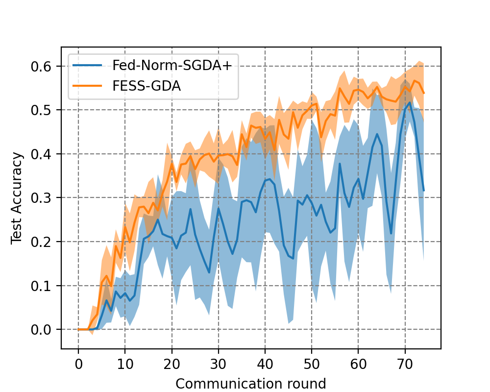
Figure 3: Comparison between Fed-Norm-SGDA+ and FESS-GDA for the worst test accuracy over 10 categories of CIFAR-10.

For the fair classification task, we have presented the average test accuracy results in Section 4.2. To compare the fairness of models trained with FESS-GDA and Fed-Norm-SGDA+, following the same setting in Section 4.2, we now present the worst-case test accuracy of models over 10 categories in Figure 3. Figure 2 and Figure 3 show that models trained with FESS-GDA not only have better average test accuracy over all categories, but also have better worst-case test accuracy over all categories, which demonstrates that models trained with FESS-GDA have better overall performance as well as fairness compared to models trained with Fed-Norm-SGDA+.

Communication savings from multiple local updates

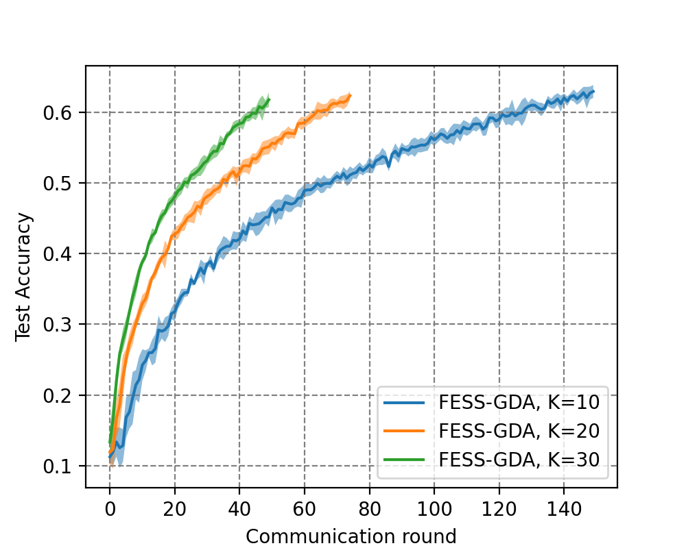
Figure 4: FESS-GDA for the fair classification task on CIFAR-10 with different number of local updates.

We test FESS-GDA for the fair classification task on CIFAR10 dataset using the same setting as in Section 4.2 with $\eta_{x,l}=\eta_{y,l}=0.1,\eta_{x,g}=\eta_{y,g}=1,p=0.1,\beta=0.9$ and number of local updates $K$ from $\{10,20,30\}$. Each experiment is repeated 5 times and we report the average performance. As we can see from Figure 4, FESS-GDA has significant communication savings from multiple local updates.

Model Architecture for Fair Classification

Table 3 shows the architecture of the convolutional neural network we used for the fair classification tasks.

Table 3: Model Architecture for CIFAR10 dataset

Layer Type	Shape	padding
Convolution $+$ ReLU	$3\times 3\times 16$	1
Max Pooling	$2\times 2$
Convolution $+$ ReLU	$3\times 3\times 32$	1
Max Pooling	$2\times 2$
Convolution $+$ ReLU	$3\times 3\times 64$	1
Max Pooling	$2\times 2$
Fully Connected $+$ ReLU	$512$
Fully Connected $+$ ReLU	$64$
Fully Connected	$10$

References

- Arjovsky et al. [2017] Martin Arjovsky, Soumith Chintala, and Léon Bottou. Wasserstein generative adversarial networks. In International conference on machine learning, pages 214–223. PMLR, 2017.
- Carbonetto et al. [2009] Peter Carbonetto, Mark Schmidt, and Nando D Freitas. An interior-point stochastic approximation method and an l1-regularized delta rule. In Advances in neural information processing systems, pages 233–240, 2009.
- Deng and Mahdavi [2021] Yuyang Deng and Mehrdad Mahdavi. Local stochastic gradient descent ascent: Convergence analysis and communication efficiency. In International Conference on Artificial Intelligence and Statistics, pages 1387–1395. PMLR, 2021.
- Deng et al. [2020a] Yuyang Deng, Mohammad Mahdi Kamani, and Mehrdad Mahdavi. Distributionally robust federated averaging. Advances in neural information processing systems, 33:15111–15122, 2020a.
- Deng et al. [2020b] Yuyang Deng, Mohammad Mahdi Kamani, and Mehrdad Mahdavi. Distributionally robust federated averaging. In Advances in Neural Information Processing Systems, volume 33, pages 15111–15122, 2020b.
- Forsgren et al. [2002] Anders Forsgren, Philip E Gill, and Margaret H Wright. Interior methods for nonlinear optimization. SIAM review, 44(4):525–597, 2002.
- Goodfellow et al. [2014a] Ian Goodfellow, Jean Pouget-Abadie, Mehdi Mirza, Bing Xu, David Warde-Farley, Sherjil Ozair, Aaron Courville, and Yoshua Bengio. Generative adversarial nets. Advances in neural information processing systems, 27, 2014a.
- Goodfellow et al. [2014b] Ian J Goodfellow, Jonathon Shlens, and Christian Szegedy. Explaining and harnessing adversarial examples. arXiv preprint arXiv:1412.6572, 2014b.
- Hou et al. [2021] Charlie Hou, Kiran K Thekumparampil, Giulia Fanti, and Sewoong Oh. Efficient algorithms for federated saddle point optimization. arXiv preprint arXiv:2102.06333, 2021.
- Jhunjhunwala et al. [2022] Divyansh Jhunjhunwala, Pranay Sharma, Aushim Nagarkatti, and Gauri Joshi. Fedvarp: Tackling the variance due to partial client participation in federated learning. In Uncertainty in Artificial Intelligence, pages 906–916. PMLR, 2022.
- Karimi et al. [2016] Hamed Karimi, Julie Nutini, and Mark Schmidt. Linear convergence of gradient and proximal-gradient methods under the polyak-łojasiewicz condition. In Machine Learning and Knowledge Discovery in Databases: European Conference, ECML PKDD 2016, Riva del Garda, Italy, September 19-23, 2016, Proceedings, Part I 16, pages 795–811. Springer, 2016.
- Krizhevsky et al. [2009] Alex Krizhevsky, Geoffrey Hinton, et al. Learning multiple layers of features from tiny images. 2009.
- Léauté and Faltings [2013] Thomas Léauté and Boi Faltings. Protecting privacy through distributed computation in multi-agent decision making. Journal of Artificial Intelligence Research, 47:649–695, 2013.
- Liang et al. [2014] Jingwei Liang, Jalal Fadili, and Gabriel Peyré. Local linear convergence of forward–backward under partial smoothness. In Advances in Neural Information Processing Systems, pages 1970–1978, 2014.
- Liao et al. [2021] Luofeng Liao, Li Shen, Jia Duan, Mladen Kolar, and Dacheng Tao. Local adagrad-type algorithm for stochastic convex-concave minimax problems. arXiv preprint arXiv:2106.10022, 2021.
- Lin et al. [2020] Tianyi Lin, Chi Jin, and Michael Jordan. On gradient descent ascent for nonconvex-concave minimax problems. In International Conference on Machine Learning, pages 6083–6093. PMLR, 2020.
- Liu et al. [2019] Mingrui Liu, Zhuoning Yuan, Yiming Ying, and Tianbao Yang. Stochastic auc maximization with deep neural networks. arXiv preprint arXiv:1908.10831, 2019.
- Loizou et al. [2020] Nicolas Loizou, Hugo Berard, Alexia Jolicoeur-Martineau, Pascal Vincent, Simon Lacoste-Julien, and Ioannis Mitliagkas. Stochastic hamiltonian gradient methods for smooth games. In International Conference on Machine Learning, pages 6370–6381. PMLR, 2020.
- Lu et al. [2019] Songtao Lu, Meisam Razaviyayn, Bo Yang, Kejun Huang, and Mingyi Hong. Snap: Finding approximate second-order stationary solutions efficiently for non-convex linearly constrained problems. arXiv preprint arXiv:1907.04450, 2019.
- Luo et al. [2020] Luo Luo, Haishan Ye, Zhichao Huang, and Tong Zhang. Stochastic recursive gradient descent ascent for stochastic nonconvex-strongly-concave minimax problems. In Advances in Neural Information Processing Systems, volume 33, pages 20566–20577, 2020.
- Madry et al. [2017] Aleksander Madry, Aleksandar Makelov, Ludwig Schmidt, Dimitris Tsipras, and Adrian Vladu. Towards deep learning models resistant to adversarial attacks. arXiv preprint arXiv:1706.06083, 2017.
- McMahan et al. [2017] Brendan McMahan, Eider Moore, Daniel Ramage, Seth Hampson, and Blaise Aguera y Arcas. Communication-efficient learning of deep networks from decentralized data. In Artificial intelligence and statistics, pages 1273–1282. PMLR, 2017.
- Namkoong and Duchi [2016] Hongseok Namkoong and John C Duchi. Stochastic gradient methods for distributionally robust optimization with f-divergences. In Advances in neural information processing systems, pages 2208–2216, 2016.
- Nouiehed et al. [2019] Maher Nouiehed, Maziar Sanjabi, Tianjian Huang, Jason D Lee, and Meisam Razaviyayn. Solving a class of non-convex min-max games using iterative first order methods. Advances in Neural Information Processing Systems, 32, 2019.
- Qiu et al. [2020] Shuang Qiu, Zhuoran Yang, Xiaohan Wei, Jieping Ye, and Zhaoran Wang. Single-timescale stochastic nonconvex-concave optimization for smooth nonlinear TD learning. arXiv preprint arXiv:2008.10103, 2020.
- Rafique et al. [2021] Hassan Rafique, Mingrui Liu, Qihang Lin, and Tianbao Yang. Weakly-convex–concave min–max optimization: provable algorithms and applications in machine learning. Optimization Methods and Software, pages 1–35, 2021.
- Reisizadeh et al. [2020] Amirhossein Reisizadeh, Farzan Farnia, Ramtin Pedarsani, and Ali Jadbabaie. Robust federated learning: The case of affine distribution shifts. In Advances in Neural Information Processing Systems, volume 33, pages 21554–21565, 2020.
- Sharma et al. [2022] Pranay Sharma, Rohan Panda, Gauri Joshi, and Pramod Varshney. Federated minimax optimization: Improved convergence analyses and algorithms. In International Conference on Machine Learning, pages 19683–19730. PMLR, 2022.
- Sharma et al. [2023] Pranay Sharma, Rohan Panda, and Gauri Joshi. Federated minimax optimization with client heterogeneity. arXiv preprint arXiv:2302.04249, 2023.
- Sun and Wei [2022] Zhenyu Sun and Ermin Wei. A communication-efficient algorithm with linear convergence for federated minimax learning. Advances in Neural Information Processing Systems, 35:6060–6073, 2022.
- Wu et al. [2023] Xidong Wu, Jianhui Sun, Zhengmian Hu, Aidong Zhang, and Heng Huang. Solving a class of non-convex minimax optimization in federated learning. arXiv preprint arXiv:2310.03613, 2023.
- Yang et al. [2021] Haibo Yang, Minghong Fang, and Jia Liu. Achieving linear speedup with partial worker participation in non-iid federated learning. arXiv preprint arXiv:2101.11203, 2021.
- Yang et al. [2022a] Haibo Yang, Zhuqing Liu, Xin Zhang, and Jia Liu. Sagda: Achieving communication complexity in federated min-max learning. Advances in Neural Information Processing Systems, 35:7142–7154, 2022a.
- Yang et al. [2020] Junchi Yang, Negar Kiyavash, and Niao He. Global convergence and variance reduction for a class of nonconvex-nonconcave minimax problems. Advances in Neural Information Processing Systems, 33:1153–1165, 2020.
- Yang et al. [2022b] Junchi Yang, Antonio Orvieto, Aurelien Lucchi, and Niao He. Faster single-loop algorithms for minimax optimization without strong concavity. In International Conference on Artificial Intelligence and Statistics, pages 5485–5517. PMLR, 2022b.
- Zhang and Luo [2020] Jiawei Zhang and Zhi-Quan Luo. A proximal alternating direction method of multiplier for linearly constrained nonconvex minimization. SIAM Journal on Optimization, 30(3):2272–2302, 2020.
- Zhang et al. [2020] Jiawei Zhang, Peijun Xiao, Ruoyu Sun, and Zhiquan Luo. A single-loop smoothed gradient descent-ascent algorithm for nonconvex-concave min-max problems. Advances in neural information processing systems, 33:7377–7389, 2020.
- Zhang et al. [2021] Kaiqing Zhang, Zhuoran Yang, and Tamer Başar. Multi-agent reinforcement learning: A selective overview of theories and algorithms. Handbook of reinforcement learning and control, pages 321–384, 2021.
- Zhang et al. [2022] Xuan Zhang, Necdet Serhat Aybat, and Mert Gurbuzbalaban. Sapd+: An accelerated stochastic method for nonconvex-concave minimax problems. arXiv preprint arXiv:2205.15084, 2022.