Gaussian Mixture Solvers for Diffusion Models

Hanzhong Guo∗1,3, Cheng Lu4, Fan Bao4, Tianyu Pang2, Shuicheng Yan2,
Chao Du†2, Chongxuan Li†1,3
1Gaoling School of Artificial Intelligence, Renmin University of China
2Sea AI Lab, Singapore
3Beijing Key Laboratory of Big Data Management and Analysis Methods, Beijing, China
4Tsinghua University
{allanguo, tianyupang, yansc, duchao}@sea.com;
lucheng.lc15@gmail.com; bf19@mails.tsinghua.edu.cn;
chongxuanli@ruc.edu.cn
Work done during an internship at Sea AI Lab. Correspondence to Chao Du and Chongxuan Li.
Abstract

Recently, diffusion models have achieved great success in generative tasks. Sampling from diffusion models is equivalent to solving the reverse diffusion stochastic differential equations (SDEs) or the corresponding probability flow ordinary differential equations (ODEs). In comparison, SDE-based solvers can generate samples of higher quality and are suited for image translation tasks like stroke-based synthesis. During inference, however, existing SDE-based solvers are severely constrained by the efficiency-effectiveness dilemma. Our investigation suggests that this is because the Gaussian assumption in the reverse transition kernel is frequently violated (even in the case of simple mixture data) given a limited number of discretization steps. To overcome this limitation, we introduce a novel class of SDE-based solvers called Gaussian Mixture Solvers (GMS) for diffusion models. Our solver estimates the first three-order moments and optimizes the parameters of a Gaussian mixture transition kernel using generalized methods of moments in each step during sampling. Empirically, our solver outperforms numerous SDE-based solvers in terms of sample quality in image generation and stroke-based synthesis in various diffusion models, which validates the motivation and effectiveness of GMS. Our code is available at https://github.com/Guohanzhong/GMS.
1 Introduction

In recent years, deep generative models and especially (score-based) diffusion models [35, 14, 37, 18] have made remarkable progress in various domains, including image generation [15, 7], audio generation [22, 32], video generation [16], 3D object generation [31], multi-modal generation [42, 5, 12, 43], and several downstream tasks such as image translation [28, 45] and image restoration [19].

Sampling from diffusion models can be interpreted as solving the reverse-time diffusion stochastic differential equations (SDEs) or their corresponding probability flow ordinary differential equations (ODEs) [37]. SDE-based and ODE-based solvers of diffusion models have very different properties and application scenarios In particular, SDE-based solvers usually perform better when given a sufficient number of discretization steps [18]. Indeed, a recent empirical study [24] suggests that SDE-based solvers can potentially generate high-fidelity samples with realistic details and intricate semantic coherence from pre-trained large-scale text-to-image diffusion models [34]. Besides, SDE-based solvers are preferable in many downstream tasks such as stroke-based synthesis [27], image translation [45], and image manipulation [20].

Despite their wide applications, SDE-based solvers face a significant trade-off between efficiency and effectiveness during sampling, since an insufficient number of steps lead to larger discretization errors. To this end, Bao et al. [3] estimate the optimal variance of the Gaussian transition kernel in the reverse process instead of using a handcraft variance to reduce the discretization errors. Additionally, Bao et al. [2] explore the optimal diagonal variance when dealing with an imperfect noise network and demonstrate state-of-the-art (SOTA) performance with a few steps among other SDE-based solvers. Notably, these solvers all assume that the transition kernel in the reverse process is Gaussian.

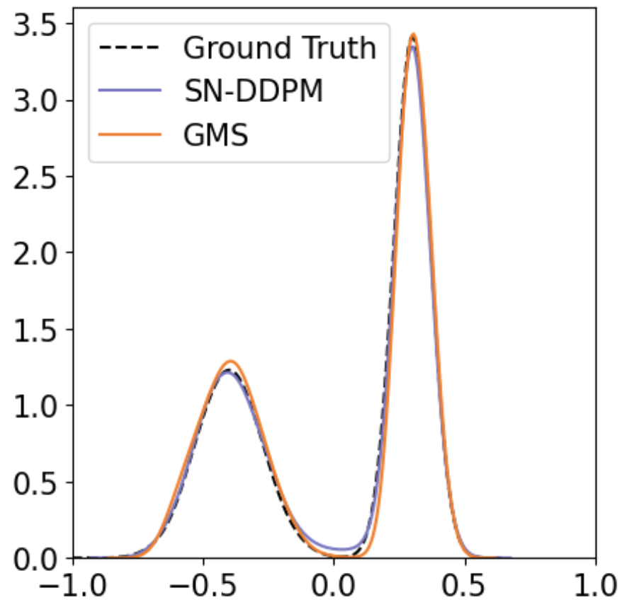
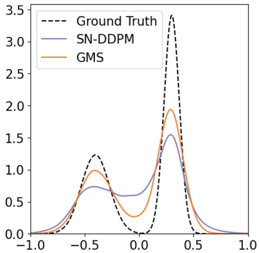
In this paper, we systematically examine the assumption of the Gaussian transition kernel and reveal that it can be easily violated under a limited number of discretization steps even in the case of simple mixture data. To this end, we propose a new type of SDE-based solver called Gaussian Mixture Solver (GMS), which employs a more expressive Gaussian mixture transition kernel in the reverse process for better approximation given a limited number of steps (see visualization results on toy data in Fig. 1). In particular, we first learn a noise prediction network with multiple heads that estimate the high-order moments of the true reverse transition kernel respectively. For sampling, we fit a Gaussian mixture transition kernel in each step via the generalized methods of the moments [11] using the predicted high-order moments of the true reverse process.

To evaluate GMS, we compare it against a variety of baselines [14, 2, 17, 36] in terms of several widely used metrics (particularly sample quality measured by FID) in the tasks of generation and stroke-based synthesis on multiple datasets. Our results show that GMS outperforms state-of-the-art SDE-based solvers [14, 2, 17] in terms of sample quality with the limited number of discretization steps (e.g., <100absent100<100). For instance, GMS improves the FID by 4.44 over the SOTA SDE-based solver [2] given 10 steps on CIFAR10. Furthermore, We evaluate GMS on a stroke-based synthesis task. The findings consistently reveal that GMS achieves higher levels of realism than all aforementioned SDE-based solvers as well as the widely adopted ODE-based solver DDIM [36] while maintaining comparable computation budgets and faithfulness scores (measured by L2subscript𝐿2L_{2} distance). Such empirical findings validate the motivation and effectiveness of GMS.

Refer to caption
(a) ##\#Step=5
Refer to caption
(b) ##\#Step=10
Refer to caption
(c) ##\#Step=20
Figure 1: Sampling on a mixture of Gaussian. GMS (ours) and SN-DDPM excel in fitting the true distribution when the transition kernel is Gaussian, with a sufficient number of sampling steps (c). However, GMS outperforms SN-DDPM [2] when sampling steps are limited and the reverse transition kernel deviates from Gaussian (a-b).

2 Background

In this section, we provide a brief overview of the (score-based) diffusion models, representative SDE-based solvers for diffusion models, and applications of such solvers.

2.1 Diffusion models

Diffusion models gradually perturb data with a forward diffusion process and then learn to reverse such process to recover the data distribution. Formally, let x0nsubscript𝑥0superscript𝑛x_{0}\in\mathbb{R}^{n} be a random variable with unknown data distribution q(x0)𝑞subscript𝑥0q(x_{0}). Diffusion models define the forward process {xt}t[0,1]subscriptsubscript𝑥𝑡𝑡01\left\{x_{t}\right\}_{t\in[0,1]} indexed by time t𝑡t, which perturbs the data by adding Gaussian noise to x0subscript𝑥0x_{0} with

q(xt|x0)=𝒩(xt|a(t)x0,σ2(t)I).𝑞conditionalsubscript𝑥𝑡subscript𝑥0𝒩conditionalsubscript𝑥𝑡𝑎𝑡subscript𝑥0superscript𝜎2𝑡𝐼\displaystyle q(x_{t}|x_{0})=\mathcal{N}(x_{t}|a(t)x_{0},\sigma^{2}(t)I). (1)

In general, the function a(t)𝑎𝑡a(t) and σ(t)𝜎𝑡\sigma(t) are selected so that the logarithmic signal-to-noise ratio loga2(t)σ2(t)superscript𝑎2𝑡superscript𝜎2𝑡\log\frac{a^{2}(t)}{\sigma^{2}(t)} decreases monotonically with time t𝑡t, causing the data to diffuse towards random Gaussian noise [21]. Furthermore, it has been demonstrated by Kingma et al. [21] that the following SDE shares an identical transition distribution qt|0(xt|x0)subscript𝑞conditional𝑡0conditionalsubscript𝑥𝑡subscript𝑥0q_{t|0}(x_{t}|x_{0}) with Eq. (1):

dxt=f(t)xtdt+g(t)dω,x0q(x0),formulae-sequencesubscript𝑥𝑡𝑓𝑡subscript𝑥𝑡𝑡𝑔𝑡𝜔similar-tosubscript𝑥0𝑞subscript𝑥0\displaystyle\differential x_{t}=f(t)x_{t}\differential t+g(t)\differential\omega,\quad x_{0}\sim q(x_{0}), (2)

where ωn𝜔superscript𝑛\omega\in\mathbb{R}^{n} is a standard Wiener process and

f(t)=dloga(t)dt,g2(t)=dσ2(t)dt2σ2(t)dloga(t)dt.formulae-sequence𝑓𝑡𝑎𝑡𝑡superscript𝑔2𝑡superscript𝜎2𝑡𝑡2superscript𝜎2𝑡𝑎𝑡𝑡\displaystyle f(t)=\frac{\differential\log a(t)}{\differential t},\quad g^{2}(t)=\frac{\differential\sigma^{2}(t)}{\differential t}-2\sigma^{2}(t)\frac{\differential\log a(t)}{\differential t}. (3)

Let q(xt)𝑞subscript𝑥𝑡q(x_{t}) be the marginal distribution of the above SDE at time t𝑡t. Its reversal process can be described by a corresponding continuous SDE which recovers the data distribution [37]:

dx=[f(t)xtg2(t)xtlogq(xt)]dt+g(t)dω¯,x1q(x1),formulae-sequence𝑥delimited-[]𝑓𝑡subscript𝑥𝑡superscript𝑔2𝑡subscriptsubscript𝑥𝑡𝑞subscript𝑥𝑡𝑡𝑔𝑡¯𝜔similar-tosubscript𝑥1𝑞subscript𝑥1\displaystyle\differential x=\left[f(t)x_{t}-g^{2}(t)\nabla_{x_{t}}\log q(x_{t})\right]\differential t+g(t)\differential\bar{\omega},\quad x_{1}\sim q(x_{1}), (4)

where ω¯n¯𝜔superscript𝑛\bar{\omega}\in\mathbb{R}^{n} is a reverse-time standard Wiener process. The only unknown term in Eq. (4) is the score function xtlogq(xt)subscriptsubscript𝑥𝑡𝑞subscript𝑥𝑡\nabla_{x_{t}}\log q(x_{t}). To estimate it, existing works [14, 37, 18] train a noise network ϵθ(xt,t)subscriptitalic-ϵ𝜃subscript𝑥𝑡𝑡\epsilon_{\theta}(x_{t},t) to obtain a scaled score function σ(t)xtlogq(xt)𝜎𝑡subscriptsubscript𝑥𝑡𝑞subscript𝑥𝑡\sigma(t)\nabla_{x_{t}}\log q(x_{t}) using denoising score matching [38]:

(θ)=01w(t)𝔼q(x0)𝔼q(ϵ)[ϵθ(xt,t)ϵ22]dt,𝜃superscriptsubscript01𝑤𝑡subscript𝔼𝑞subscript𝑥0subscript𝔼𝑞italic-ϵdelimited-[]superscriptsubscriptnormsubscriptitalic-ϵ𝜃subscript𝑥𝑡𝑡italic-ϵ22𝑡\displaystyle\mathcal{L}(\theta)=\int_{0}^{1}w(t)\mathbb{E}_{q(x_{0})}\mathbb{E}_{q(\epsilon)}[\left\|\epsilon_{\theta}(x_{t},t)-\epsilon\right\|_{2}^{2}]\differential t, (5)

where w(t)𝑤𝑡w(t) is a weighting function, q(ϵ)𝑞italic-ϵq(\epsilon) is standard Gaussian distribution and xtq(xt|x0)similar-tosubscript𝑥𝑡𝑞conditionalsubscript𝑥𝑡subscript𝑥0x_{t}\sim q(x_{t}|x_{0}) follows Eq. (1). The optimal solution of the optimization objective Eq. (5) is ϵθ(xt,t)=σ(t)xtlogq(xt)subscriptitalic-ϵ𝜃subscript𝑥𝑡𝑡𝜎𝑡subscriptsubscript𝑥𝑡𝑞subscript𝑥𝑡\epsilon_{\theta}(x_{t},t)=-\sigma(t)\nabla_{x_{t}}\log q(x_{t}).

Hence, samples can be obtained by initiating the process with a standard Gaussian variable x1subscript𝑥1x_{1}, then substituting xtlogq(xt)subscriptsubscript𝑥𝑡𝑞subscript𝑥𝑡\nabla_{x_{t}}\log q(x_{t}) with ϵθ(xt,t)σ(t)subscriptitalic-ϵ𝜃subscript𝑥𝑡𝑡𝜎𝑡-\frac{\epsilon_{\theta}(x_{t},t)}{\sigma(t)} and discretizing reverse SDE Eq. (4) from t=1𝑡1t=1 to t=0𝑡0t=0 to generate x0subscript𝑥0x_{0}.

2.2 SDE-based solvers for diffusion models

The primary objective of SDE-based solvers lies in decreasing discretization error and therefore minimizing function evaluations required for convergence during the process of discretizing Eq. (4). Discretizing the reverse SDE in Eq. (4) is equivalent to sample from a Markov chain p(x0:1)=p(x1)ti1,tiStp(xti1|xti)𝑝subscript𝑥:01𝑝subscript𝑥1subscriptproductsubscript𝑡𝑖1subscript𝑡𝑖subscript𝑆𝑡𝑝conditionalsubscript𝑥subscript𝑡𝑖1subscript𝑥subscript𝑡𝑖p(x_{0:1})=p(x_{1})\prod_{t_{i-1},t_{i}\in S_{t}}p(x_{t_{i-1}}|x_{t_{i}}) with its trajectory St=[0,t1,t2,,ti,..,1]S_{t}=[0,t_{1},t_{2},...,t_{i},..,1].  Song et al. [37] proves that the conventional ancestral sampling technique used in the DPMs [14] that models p(xti1|xti)𝑝conditionalsubscript𝑥subscript𝑡𝑖1subscript𝑥subscript𝑡𝑖p(x_{t_{i-1}}|x_{t_{i}}) as a Gaussian distribution, can be perceived as a first-order solver for the reverse SDE in Eq. (4)italic-(4italic-)\eqref{eq:continuous_back}.  Bao et al. [3] finds that the optimal variance of p(xti1|xti)𝒩(xti1|μti1|ti,Σti1|ti(xti))similar-to𝑝conditionalsubscript𝑥subscript𝑡𝑖1subscript𝑥subscript𝑡𝑖𝒩conditionalsubscript𝑥subscript𝑡𝑖1subscript𝜇conditionalsubscript𝑡𝑖1subscript𝑡𝑖subscriptΣconditionalsubscript𝑡𝑖1subscript𝑡𝑖subscript𝑥subscript𝑡𝑖p(x_{t_{i-1}}|x_{t_{i}})\sim\mathcal{N}(x_{t_{i-1}}|\mu_{t_{i-1}|t_{i}},\Sigma_{t_{i-1}|t_{i}}(x_{t_{i}})) is

Σti1|ti(xti)=λti2+γti2σ2(ti)α(ti)(1𝔼q(xti)[1d𝔼q(x0|xti)[ϵθ(xti,ti)]22]),subscriptsuperscriptΣconditionalsubscript𝑡𝑖1subscript𝑡𝑖subscript𝑥subscript𝑡𝑖superscriptsubscript𝜆subscript𝑡𝑖2superscriptsubscript𝛾subscript𝑡𝑖2superscript𝜎2subscript𝑡𝑖𝛼subscript𝑡𝑖1subscript𝔼𝑞subscript𝑥subscript𝑡𝑖delimited-[]1𝑑superscriptsubscriptnormsubscript𝔼𝑞conditionalsubscript𝑥0subscript𝑥subscript𝑡𝑖delimited-[]subscriptitalic-ϵ𝜃subscript𝑥subscript𝑡𝑖subscript𝑡𝑖22\displaystyle\Sigma^{*}_{t_{i-1}|t_{i}}(x_{t_{i}})=\lambda_{t_{i}}^{2}+\gamma_{t_{i}}^{2}\frac{\sigma^{2}(t_{i})}{\alpha(t_{i})}\left(1-\mathbb{E}_{q(x_{t_{i}})}\left[\frac{1}{d}\left\|\mathbb{E}_{q(x_{0}|x_{t_{i}})}[\epsilon_{\theta}(x_{t_{i}},t_{i})]\right\|_{2}^{2}\right]\right), (6)

where, γti=α(ti1)σ2(ti1)λti2α(ti)σ2(ti)subscript𝛾subscript𝑡𝑖𝛼subscript𝑡𝑖1superscript𝜎2subscript𝑡𝑖1subscriptsuperscript𝜆2subscript𝑡𝑖𝛼subscript𝑡𝑖superscript𝜎2subscript𝑡𝑖\gamma_{t_{i}}=\sqrt{\alpha(t_{i-1})}-\sqrt{\sigma^{2}(t_{i-1})-\lambda^{2}_{t_{i}}}\sqrt{\frac{\alpha(t_{i})}{\sigma^{2}(t_{i})}}, λti2superscriptsubscript𝜆subscript𝑡𝑖2\lambda_{t_{i}}^{2} is the variance of q(xti1|xti,x0)𝑞conditionalsubscript𝑥subscript𝑡𝑖1subscript𝑥subscript𝑡𝑖subscript𝑥0q(x_{t_{i-1}}|x_{t_{i}},x_{0}). AnalyticDPM [3] offers a significant reduction in discretization error during sampling and achieves faster convergence with fewer steps. Moreover, SN-DDPM [2] employs a Gaussian transition kernel with an optimal diagonal covariance instead of an isotropic covariance. This approach yields improved sample quality and likelihood compared to other SDE-based solvers within a limited number of steps.

2.3 Applications of SDE-based solvers for stroke-based synthesis

The stroke-based image synthesis is a representative downstream task suitable for SDE-based solvers. It involves the user providing a full-resolution image x(g)superscript𝑥𝑔x^{(g)} through the manipulation of RGB pixels, referred to as the guided image. The guided image x(g)superscript𝑥𝑔x^{(g)} possibly contains three levels of guidance: a high-level guide consisting of coarse colored strokes, a mid-level guide comprising colored strokes on a real image, and a low-level guide containing image patches from a target image.

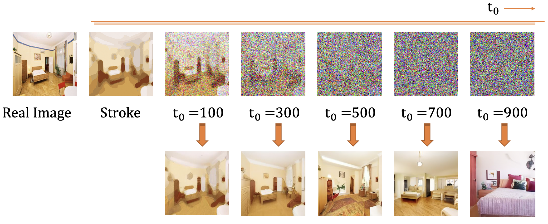
SDEdit [27] solves the task by first starting from the guided image x(g)superscript𝑥𝑔x^{(g)} and adding Gaussian noise to disturb the guided images to xtsubscript𝑥𝑡x_{t} and q(x(g)(t0)|x(g))𝒩(xt0|a(t0)x(g),σ2(t)I)similar-to𝑞conditionalsuperscript𝑥𝑔subscript𝑡0superscript𝑥𝑔𝒩conditionalsubscript𝑥subscript𝑡0𝑎subscript𝑡0superscript𝑥𝑔superscript𝜎2𝑡𝐼q(x^{(g)}(t_{0})|x^{(g)})\sim\mathcal{N}(x_{t_{0}}|a(t_{0})x^{(g)},\sigma^{2}(t)I) same with Eq. (1). Subsequently, it solves the corresponding reverse stochastic differential equation (SDE) up to t=0𝑡0t=0 to generate the synthesized image x(0)𝑥0x(0) discretizing Eq. (4). Apart from the discretization steps taken by the SDE-based solver, the key hyper-parameter for SDEdit is t0subscript𝑡0t_{0}, the time step from which we begin the image synthesis procedure in the reverse SDE.

3 Gaussian mixture solvers for diffusion models

In this section, we first show through both theoretical and empirical evidence, that the true reverse transition kernel can significantly diverge from Gaussian distributions as assumed in previous SOTA SDE-based solvers [3, 2], indicating that the reverse transition can be improved further by employing more flexible distributions (see Sec. 3.1). This motivates us to propose a novel class of SDE-based solvers, dubbed Gaussian Mixture Solvers, which determines a Gaussian mixture distribution via the generalized methods of the moments [11] using higher-order moments information for the true reverse transition (see Sec. 3.2). The higher-order moments are estimated by a noise prediction network with multiple heads on training data, as detailed in Sec. 3.3.

3.1 Suboptimality of Gaussian distributions for reverse transition kernels

As described in Sec. 2, existing state-of-the-art SDE-based solvers for DPMs [3, 2] approximate the reverse transition q(xti1|xti)𝑞conditionalsubscript𝑥subscript𝑡𝑖1subscript𝑥subscript𝑡𝑖q(x_{t_{i-1}}|x_{t_{i}}) using Gaussian distributions. Such approximations work well when the number of discretization steps in these solvers is large (e.g., 100010001000 steps). However, for smaller discretization steps (such as when faster sampling is required), the validity of this Gaussian assumption will be largely broken. We demonstrate this theoretically and empirically below.

First, observe that q(xs|xt)𝑞conditionalsubscript𝑥𝑠subscript𝑥𝑡q(x_{s}|x_{t})111To enhance the clarity of exposition, we introduce the notation sti1approaches-limit𝑠subscript𝑡𝑖1s\doteq t_{i-1} and ttiapproaches-limit𝑡subscript𝑡𝑖t\doteq t_{i} to denote two adjacent time steps in the trajectory. Consequently, we refer to q(xs|xt)𝑞conditionalsubscript𝑥𝑠subscript𝑥𝑡q(x_{s}|x_{t}) as the reverse transition kernel in this context. can be expressed as q(xs|xt)=q(xs|xt,x0)q(x0|xt)dx0𝑞conditionalsubscript𝑥𝑠subscript𝑥𝑡𝑞conditionalsubscript𝑥𝑠subscript𝑥𝑡subscript𝑥0𝑞conditionalsubscript𝑥0subscript𝑥𝑡subscript𝑥0q(x_{s}|x_{t})=\int q(x_{s}|x_{t},x_{0})q(x_{0}|x_{t})\differential x_{0}, which is non-Gaussian for a general data distribution q(x0)𝑞subscript𝑥0q(x_{0}). For instance, for a mixture of Gaussian or a mixture of Dirac q(x0)𝑞subscript𝑥0q(x_{0}), we can prove that the conditional distributions q(xs|xt)𝑞conditionalsubscript𝑥𝑠subscript𝑥𝑡q(x_{s}|x_{t}) in the reverse process are non-Gaussian, as characterized by Proposition 3.1, proven in Appendix A.1.

Proposition 3.1 (Mixture Data Have non-Gaussian Reverse Kernel).

Assume q(x0)𝑞subscript𝑥0q(x_{0}) is a mixture of Dirac or a mixture of Gaussian distribution and the forward process is defined in Eq. (1). The reverse transition kernel q(xs|xt),s<t𝑞conditionalsubscript𝑥𝑠subscript𝑥𝑡𝑠𝑡q(x_{s}|x_{t}),s<t is a Gaussian mixture instead of a Gaussian.
Refer to caption
(a) logarithm mean of L2subscript𝐿2L_{2}-norm
Refer to caption
(b) logarithm median of L2subscript𝐿2L_{2}-norm
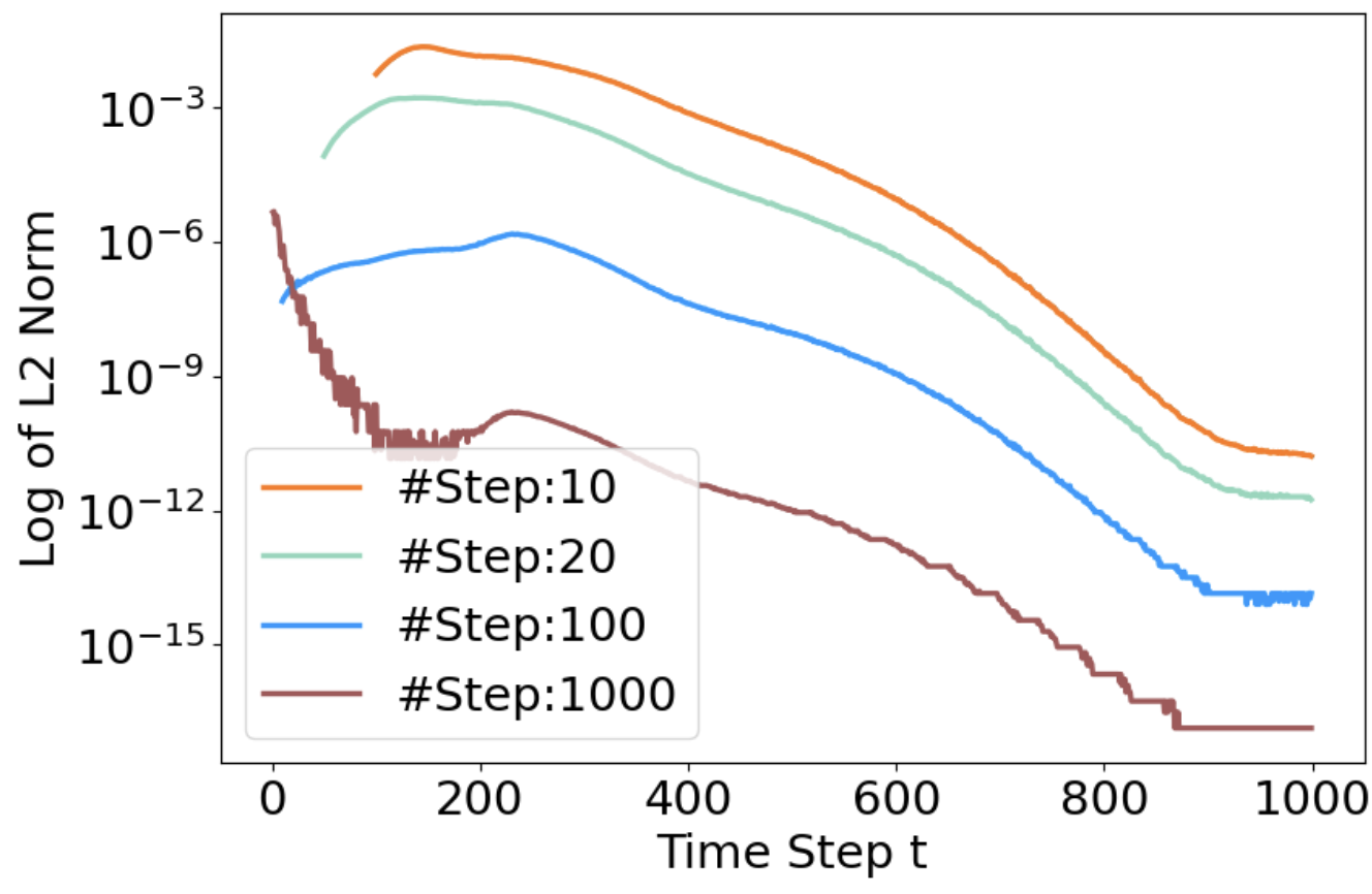
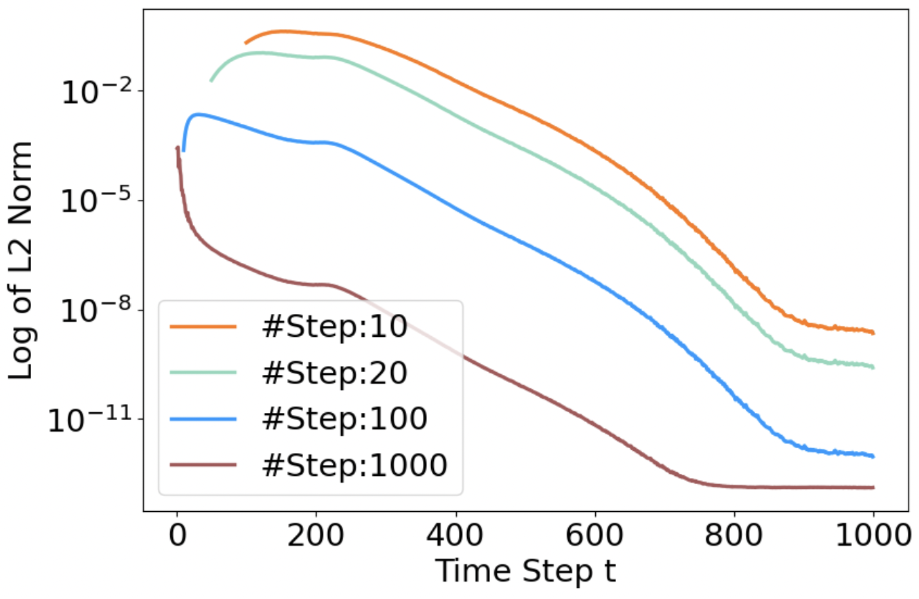
Figure 2: Empirical evidence of suboptimality of Gaussian kernel on CIFAR10. (a) and (b) plot the logarithm of the image-wise mean and median of L2subscript𝐿2L_{2}-norm between Gaussian-assumed third-order moments and estimated third-order moments. Clearly, as the number of sampling steps decreases, the disparity between the following two third-order moments increases, denoting that the true transition kernel diverges further from the Gaussian distribution. See Appendix D.2 for more details.

Empirically, we do not know the distributions of the real data (e.g., high-dimensional images) and cannot obtain an explicit form of q(xs|xt)𝑞conditionalsubscript𝑥𝑠subscript𝑥𝑡q(x_{s}|x_{t}). However, even in such cases, it is easy to validate that q(xs|xt)𝑞conditionalsubscript𝑥𝑠subscript𝑥𝑡q(x_{s}|x_{t}) are non-Gaussian. In particular, note that the third-order moment of one Gaussian distribution (M3(G)superscriptsubscript𝑀3𝐺M_{3}^{(G)}) can be represented by its first-order moment (M1subscript𝑀1M_{1}) and its second-order moment (M2subscript𝑀2M_{2}222The scalar case is M3(G)=M13+3M1(M2M12)superscriptsubscript𝑀3𝐺superscriptsubscript𝑀133subscript𝑀1subscript𝑀2superscriptsubscript𝑀12M_{3}^{(G)}=M_{1}^{3}+3M_{1}(M_{2}-M_{1}^{2}). See Appendix D.2 for the vector case., which motivates us to check whether the first three order moments of q(xs|xt)𝑞conditionalsubscript𝑥𝑠subscript𝑥𝑡q(x_{s}|x_{t}) satisfy the relationship induced by the Gaussian assumption. We perform an experiment on CIFAR-10 and estimate the first three orders of moments M1^^subscript𝑀1\hat{M_{1}}, M2^^subscript𝑀2\hat{M_{2}}, M^3subscript^𝑀3\hat{M}_{3} for q(xs|xt)𝑞conditionalsubscript𝑥𝑠subscript𝑥𝑡q(x_{s}|x_{t}) from data by high-order noise networks (see details in Sec. D.2). As shown in Fig. 2, we plot the mean and median of l2subscript𝑙2l_{2}-norm between the estimated third-order moment M3^^subscript𝑀3\hat{M_{3}} and third-order moment M3(G)superscriptsubscript𝑀3𝐺M_{3}^{(G)} calculated under the Gaussian assumption given the different number of steps at different time steps t𝑡t. In particular, when the number of steps is large (i.e., ##\#Step=100010001000), the difference between the two calculation methods is small. As the number of steps decreases, the l2subscript𝑙2l_{2}-norm increases, indicating that the true reverse distribution q(xs|xt)𝑞conditionalsubscript𝑥𝑠subscript𝑥𝑡q(x_{s}|x_{t}) is non-Gaussian. With the time step closer to t=0𝑡0t=0, the l2subscript𝑙2l_{2}-norm increases too.

Both the theoretical and empirical results motivate us to weaken the Gaussian assumption in SDE-based solvers for better performance, especially when the step size is large.

3.2 Sampling with Gaussian mixture transition kernel

There are extensive choices of p(xs|xt)𝑝conditionalsubscript𝑥𝑠subscript𝑥𝑡p(x_{s}|x_{t}) such that it is more powerful and potentially fits q(xs|xt)𝑞conditionalsubscript𝑥𝑠subscript𝑥𝑡q(x_{s}|x_{t}) better than a Gaussian. In this paper, we choose a simple mixture of the Gaussian model as follows:

p(xs|xt)=i=1Mwi𝒩(xs|μi(xt),Σi(xt)),i=1Mwi=1,formulae-sequence𝑝conditionalsubscript𝑥𝑠subscript𝑥𝑡superscriptsubscript𝑖1𝑀subscript𝑤𝑖𝒩conditionalsubscript𝑥𝑠subscript𝜇𝑖subscript𝑥𝑡subscriptΣ𝑖subscript𝑥𝑡superscriptsubscript𝑖1𝑀subscript𝑤𝑖1\displaystyle p(x_{s}|x_{t})=\sum_{i=1}^{M}w_{i}\mathcal{N}(x_{s}|{\mu_{i}}(x_{t}),{\Sigma_{i}}(x_{t})),\quad\sum_{i=1}^{M}w_{i}=1, (7)

where wisubscript𝑤𝑖w_{i} is a scalar and μi(xt)subscript𝜇𝑖subscript𝑥𝑡\mu_{i}(x_{t}) and Σi(xt)subscriptΣ𝑖subscript𝑥𝑡\Sigma_{i}(x_{t}) are vectors. The reasons for choosing a Gaussian mixture model are three-fold. First, a Gaussian mixture model is multi-modal (e.g., see Proposition 3.1), potentially leading to a better performance than Gaussian with few steps. Second, when the number of steps is large and the Gaussian is nearly optimal [35, 3], a designed Gaussian mixture model such as our proposed kernel in Eq. (9) can degenerate to a Gaussian when the mean of two components are same, making the performance unchanged. Third, a Gaussian mixture model is relatively easy to sample. For the sake of completeness, we also discuss other distribution families in Appendix C.

Traditionally, the EM algorithm is employed for estimating the Gaussian mixture [26]. However, it is nontrivial to apply EM here because we need to learn the reverse transition kernel in Eq. (7) for all time step pairs (s,t)𝑠𝑡(s,t) by individual EM processes where we need to sample multiple xssubscript𝑥𝑠x_{s}333Note that xssubscript𝑥𝑠x_{s} serves as the “training sample” in the corresponding EM process. given a xtsubscript𝑥𝑡x_{t} to estimate the parameters in the Gaussian mixture indexed by (s,t)𝑠𝑡(s,t). This is time-consuming, especially in a high-dimensional space (e.g., natural images) and we present an efficient approach.

For improved flexibility in sampling and training, diffusion models introduce the parameterization of the noise network ϵ(xt,t)italic-ϵsubscript𝑥𝑡𝑡\epsilon(x_{t},t) [14] or the data prediction network x0(xt,t)subscript𝑥0subscript𝑥𝑡𝑡x_{0}(x_{t},t) [18]. With such a network, the moments under the q(xs|xt)𝑞conditionalsubscript𝑥𝑠subscript𝑥𝑡q(x_{s}|x_{t}) measure can be decomposed into moments under the q(x0|xt)𝑞conditionalsubscript𝑥0subscript𝑥𝑡q(x_{0}|x_{t}) measure so that sampling any xtsubscript𝑥𝑡x_{t} to xssubscript𝑥𝑠x_{s} requires only a network whose inputs are xtsubscript𝑥𝑡x_{t} and t𝑡t, such as the decomposition shown in Eq. (10). In previous studies, Gaussian transition kernel was utilized, allowing for the distribution to be directly determined after obtaining the estimated first-order moment and handcrafted second-order moment [14] or estimated first-order and second-order moment [3]. In contrast, such a feature is not available for the Gaussian mixtures transition kernel in our paper.

Here we present the method to determine the Gaussian mixture given a set of moments and we will discuss how to obtain the moments by the parameterization of the noise network in Sec. 3.3. Assume the length of the estimated moments set is N𝑁N and the number of parameters in the Gaussian mixture is d𝑑d. We adopt a popular and theoretically sound method called the generalized method of moments (GMM) [11] to learn the parameters by:

minθQ(θ,M1,,MN)=minθ[1Nci=1Ncg(xi,θ)]TW[1Nci=1Ncg(xi,θ)],\displaystyle\small\min_{\theta}Q(\theta,M_{1},...,M_{N})=\min_{\theta}[\frac{1}{N_{c}}\sum_{i=1}^{N_{c}}g(x_{i},\theta)]^{T}W[\frac{1}{N_{c}}\sum_{i=1}^{N_{c}}g(x_{i},\theta)], (8)

where θd×1𝜃superscript𝑑1\theta\in\mathbb{R}^{d\times 1} includes all parameters (e.g., the mean of each component) in the Gaussian mixture defined in Eq. (7). For instance, d=2MDdata+M1𝑑2𝑀subscript𝐷data𝑀1d=2M*D_{\textrm{data}}+M-1 in Eq. (7), where Ddatasubscript𝐷dataD_{\textrm{data}} represents the number of dimensions of the data and θ𝜃\theta contains M𝑀M mean vectors with Ddatasubscript𝐷dataD_{\textrm{data}} dimensions, M𝑀M variance vectors of with Ddatasubscript𝐷dataD_{\textrm{data}} dimensions (considering only the diagonal elements), and M1𝑀1M-1 weight coefficients which are scalar. The component of g(xi,θ)N×1𝑔subscript𝑥𝑖𝜃superscript𝑁1g(x_{i},\theta)\in\mathbb{R}^{N\times 1} is defined by gn(xi,θ)=Mn(xi)Mn(GM)(θ)subscript𝑔𝑛subscript𝑥𝑖𝜃subscript𝑀𝑛subscript𝑥𝑖superscriptsubscript𝑀𝑛𝐺𝑀𝜃g_{n}(x_{i},\theta)=M_{n}(x_{i})-M_{n}^{(GM)}(\theta), where Mn(xi)subscript𝑀𝑛subscript𝑥𝑖M_{n}(x_{i}) is the n𝑛n-th order empirical moments stated in Sec. 3.3 and Mn(GM)(θ)superscriptsubscript𝑀𝑛𝐺𝑀𝜃M_{n}^{(GM)}(\theta) is the n𝑛n-th order moments of Gaussian mixture under θ𝜃\theta, and W𝑊W is a weighted matrix, Ncsubscript𝑁𝑐N_{c} is the number of samples.

Theoretically, the parameter θ^GMMsubscript^𝜃GMM\hat{\theta}_{\textrm{GMM}} obtained by GMM in Eq. (8) consistently converges to the potential optimal parameters θsuperscript𝜃\theta^{*} for Gaussian mixture models given the moments’ condition because Nc(θ^GMMθ)𝑑𝒩(0,𝕍(θGMM))subscript𝑁𝑐subscript^𝜃GMMsuperscript𝜃𝑑𝒩0𝕍subscript𝜃𝐺𝑀𝑀\sqrt{N_{c}}(\hat{\theta}_{\textrm{GMM}}-\theta^{*})\overset{d}{\rightarrow}\mathcal{N}(0,\mathbb{V}(\theta_{GMM})), as stated in Theorem 3.1 in Hansen [11].

Hence, we can employ GMM to determine a Gaussian mixture transition kernel after estimating the moments of the transition kernel. To strike a balance between computational tractability and expressive power, we specifically focus on the first three-order moments in this work and define a Gaussian mixture transition kernel with two components shown in Eq. (9) whose vectors μt(1)subscriptsuperscript𝜇1𝑡\mu^{(1)}_{t}, μt(2)subscriptsuperscript𝜇2𝑡\mu^{(2)}_{t}, and σt2subscriptsuperscript𝜎2𝑡\sigma^{2}_{t} are parameters to be optimized. This degree of simplification is acceptable in terms of its impact. Intuitively, such a selection has the potential to encompass exponential modes throughout the entire trajectory. Empirically, we consistently observe that utilizing a bimodal Gaussian mixture yields favorable outcomes across all experimental configurations.

p(xs|xt)=13𝒩(μt(1),σt2)+23𝒩(μt(2),σt2),𝑝conditionalsubscript𝑥𝑠subscript𝑥𝑡13𝒩subscriptsuperscript𝜇1𝑡subscriptsuperscript𝜎2𝑡23𝒩subscriptsuperscript𝜇2𝑡subscriptsuperscript𝜎2𝑡\displaystyle p(x_{s}|x_{t})=\frac{1}{3}\mathcal{N}({\mu^{(1)}_{t}},{\sigma^{2}_{t}})+\frac{2}{3}\mathcal{N}({\mu^{(2)}_{t}},{\sigma^{2}_{t}}), (9)

meanwhile, under the simplification in our paper, the number of parameters d=3Ddata𝑑3subscript𝐷datad=3*D_{\textrm{data}} in our Gaussian transition kernel is equal to the number of moments condition N=3Ddata𝑁3subscript𝐷dataN=3*D_{\textrm{data}}. According to proposition 3.2, under the selection of arbitrary weighted weights, the asymptotic mean (asymptotically consistent) and asymptotic variance of the estimator remain consistent, proof in Appendix A.2. Hence, any choice of weighted weights is optimal. To further streamline optimization, we set W=I𝑊𝐼W=I.

Proposition 3.2 (Any weighted matrix is optimal for d=N𝑑𝑁d=N).

Assume the number of parameters d𝑑d equals the number of moments condition N𝑁N, and ϵθn(xt,t)𝑝𝔼q(x0|xt)[diag(ϵn1ϵ)]subscriptsuperscriptitalic-ϵ𝑛𝜃subscript𝑥𝑡𝑡𝑝subscript𝔼𝑞conditionalsubscript𝑥0subscript𝑥𝑡delimited-[]diagsuperscripttensor-product𝑛1italic-ϵitalic-ϵ\epsilon^{n}_{\theta}(x_{t},t)\overset{p}{\rightarrow}\mathbb{E}_{q(x_{0}|x_{t})}[\textrm{diag}(\epsilon\otimes^{n-1}\epsilon)] (where nsuperscripttensor-product𝑛\otimes^{n} denotes n-fold outers product) which denotes n𝑛n-th order noise network converging in probability. The asymptotic variance 𝕍(θGMM)𝕍subscript𝜃𝐺𝑀𝑀\mathbb{V}(\theta_{GMM}) and the convergence speed of GMM remain the same no matter which weighted matrix is adopted in Eq. (8). Namely, any weighted matrix is optimal.

What’s more, we provide a detailed discussion on the selection of parameters such as the choice of different parameters to optimize and the different choices of weight wisubscript𝑤𝑖w_{i} in the Gaussian mixture in Appendix E.1. Combining with Sec. 4.1, our empirical findings illustrate the efficacy of the GMS across various benchmarks via using the Gaussian transition kernel in Eq. (9) fitted by the objective function shown in Eq. (31) in Appendix B.1 via the ADAN [41] as optimization method. Details regarding the parameters for this optimizer are provided in Appendix E.5.

3.3 Estimating high-order moments for non-Gaussian reverse process

In Sec. 3.2, we have explored the methodology for determining a Gaussian mixture transition kernel given a set of moments M1,,Mnsubscript𝑀1subscript𝑀𝑛M_{1},...,M_{n}. In the subsequent section, we will present an approach for estimating these moments utilizing noise networks and elucidate the process of network learning.

Given the forward process described by Eq. (1), it can be inferred that both q(xt|xs)𝑞conditionalsubscript𝑥𝑡subscript𝑥𝑠q(x_{t}|x_{s}) and q(xs|xt,x0)𝑞conditionalsubscript𝑥𝑠subscript𝑥𝑡subscript𝑥0q(x_{s}|x_{t},x_{0}) follow Gaussian distributions. Specifically, q(xt|xs)𝒩(xt|at|sxs,σt|s2I)similar-to𝑞conditionalsubscript𝑥𝑡subscript𝑥𝑠𝒩conditionalsubscript𝑥𝑡subscript𝑎conditional𝑡𝑠subscript𝑥𝑠subscriptsuperscript𝜎2conditional𝑡𝑠𝐼q(x_{t}|x_{s})\sim\mathcal{N}(x_{t}|a_{t|s}x_{s},\sigma^{2}_{t|s}I) [21], where at|s=α(t)α(s)subscript𝑎conditional𝑡𝑠𝛼𝑡𝛼𝑠a_{t|s}=\frac{\alpha(t)}{\alpha(s)} and σt|s2=σ2(t)at|s2σ2(s)superscriptsubscript𝜎conditional𝑡𝑠2superscript𝜎2𝑡superscriptsubscript𝑎conditional𝑡𝑠2superscript𝜎2𝑠\sigma_{t|s}^{2}=\sigma^{2}(t)-a_{t|s}^{2}\sigma^{2}(s). Consequently, we can deduce that 𝔼q(xs|xt)[xsnxs]=𝔼q(x0|xt)q(xs|xt,x0)[xsnxs]subscript𝔼𝑞conditionalsubscript𝑥𝑠subscript𝑥𝑡delimited-[]superscripttensor-product𝑛subscript𝑥𝑠subscript𝑥𝑠subscript𝔼𝑞conditionalsubscript𝑥0subscript𝑥𝑡𝑞conditionalsubscript𝑥𝑠subscript𝑥𝑡subscript𝑥0delimited-[]superscripttensor-product𝑛subscript𝑥𝑠subscript𝑥𝑠\mathbb{E}_{q(x_{s}|x_{t})}[x_{s}\otimes^{n}x_{s}]=\mathbb{E}_{q(x_{0}|x_{t})q(x_{s}|x_{t},x_{0})}[x_{s}\otimes^{n}x_{s}], where nsuperscripttensor-product𝑛\otimes^{n} denotes n𝑛n-fold outer product. Thus, we can first utilize the Gaussian property of q(xs|xt,x0)𝑞conditionalsubscript𝑥𝑠subscript𝑥𝑡subscript𝑥0q(x_{s}|x_{t},x_{0}) and employ an explicit formula to calculate the moments under the measure of q(xs|xt,x0)𝑞conditionalsubscript𝑥𝑠subscript𝑥𝑡subscript𝑥0q(x_{s}|x_{t},x_{0}). What’s more, we only consider the diagonal elements of higher-order moments for computational efficiency, similar to Bao et al. [2] since estimating full higher-order moments results in escalated output dimensions (e.g., quadratic growth for covariance and cubic for the third-order moments) and thus requires substantial computational demands. The expression of diagonal elements of the third-order moment of the reverse transition kernel can be derived as:

M^3=𝔼q(xs|xt)[diag(xsxsxs)]=𝔼q(x0|xt)𝔼q(xs|xt,x0)[diag(xsxsxs)]=subscript^𝑀3subscript𝔼𝑞conditionalsubscript𝑥𝑠subscript𝑥𝑡delimited-[]diagtensor-productsubscript𝑥𝑠subscript𝑥𝑠subscript𝑥𝑠subscript𝔼𝑞conditionalsubscript𝑥0subscript𝑥𝑡subscript𝔼𝑞conditionalsubscript𝑥𝑠subscript𝑥𝑡subscript𝑥0delimited-[]diagtensor-productsubscript𝑥𝑠subscript𝑥𝑠subscript𝑥𝑠absent\displaystyle\hat{M}_{3}=\mathbb{E}_{q(x_{s}|x_{t})}[\textrm{diag}(x_{s}\otimes{x_{s}}\otimes{x_{s}})]=\mathbb{E}_{q(x_{0}|x_{t})}\mathbb{E}_{q(x_{s}|x_{t},x_{0})}[\textrm{diag}(x_{s}\otimes{x_{s}}\otimes{x_{s}})]= (10)
[(at|sσs2σt2)3diag(xtxtxt)+3λt2at|sσs2σt2xt]Constant termsubscriptdelimited-[]superscriptsubscript𝑎conditional𝑡𝑠superscriptsubscript𝜎𝑠2superscriptsubscript𝜎𝑡23diagtensor-productsubscript𝑥𝑡subscript𝑥𝑡subscript𝑥𝑡3superscriptsubscript𝜆𝑡2subscript𝑎conditional𝑡𝑠superscriptsubscript𝜎𝑠2superscriptsubscript𝜎𝑡2subscript𝑥𝑡Constant term\displaystyle\underbrace{[(\frac{a_{t|s}\sigma_{s}^{2}}{\sigma_{t}^{2}})^{3}\textrm{diag}({x_{t}}\otimes{x_{t}}\otimes{x_{t}})+3\lambda_{t}^{2}\frac{a_{t|s}\sigma_{s}^{2}}{\sigma_{t}^{2}}x_{t}]}_{\textrm{Constant term}}
+[3at|s2σs4as|02βt|s2σt8(diag(xtxt))+as|0βt|sσt2I]𝔼q(x0|xt)[x0]Linear term in x0subscriptdirect-productdelimited-[]3superscriptsubscript𝑎conditional𝑡𝑠2superscriptsubscript𝜎𝑠4superscriptsubscript𝑎conditional𝑠02superscriptsubscript𝛽conditional𝑡𝑠2superscriptsubscript𝜎𝑡8diagtensor-productsubscript𝑥𝑡subscript𝑥𝑡subscript𝑎conditional𝑠0subscript𝛽conditional𝑡𝑠superscriptsubscript𝜎𝑡2𝐼subscript𝔼𝑞conditionalsubscript𝑥0subscript𝑥𝑡delimited-[]subscript𝑥0Linear term in x0\displaystyle+\underbrace{[\frac{3a_{t|s}^{2}\sigma_{s}^{4}a_{s|0}^{2}\beta_{t|s}^{2}}{\sigma_{t}^{8}}(\textrm{diag}({x_{t}}\otimes{x_{t}}))+\frac{a_{s|0}\beta_{t|s}}{\sigma_{t}^{2}}I]\odot\mathbb{E}_{q(x_{0}|x_{t})}[x_{0}]}_{\textrm{Linear term in $x_{0}$}}
+3at|sσs2σt2(as|0βt|sσt2)2xt𝔼q(x0|xt)[diag(x0x0)]Quadratic term in x0+(as|0βt|sσt2)3𝔼q(x0|xt)[diag(x0x0x0)]Cubic term in x0,subscriptdirect-product3subscript𝑎conditional𝑡𝑠superscriptsubscript𝜎𝑠2superscriptsubscript𝜎𝑡2superscriptsubscript𝑎conditional𝑠0subscript𝛽conditional𝑡𝑠superscriptsubscript𝜎𝑡22subscript𝑥𝑡subscript𝔼𝑞conditionalsubscript𝑥0subscript𝑥𝑡delimited-[]diagtensor-productsubscript𝑥0subscript𝑥0Quadratic term in x0subscriptsuperscriptsubscript𝑎conditional𝑠0subscript𝛽conditional𝑡𝑠superscriptsubscript𝜎𝑡23subscript𝔼𝑞conditionalsubscript𝑥0subscript𝑥𝑡delimited-[]diagtensor-productsubscript𝑥0subscript𝑥0subscript𝑥0Cubic term in x0\displaystyle+\underbrace{3\frac{a_{t|s}\sigma_{s}^{2}}{\sigma_{t}^{2}}(\frac{a_{s|0}\beta_{t|s}}{\sigma_{t}^{2}})^{2}x_{t}\odot\mathbb{E}_{q(x_{0}|x_{t})}[\textrm{diag}({x_{0}}\otimes{x_{0}})]}_{\textrm{Quadratic term in $x_{0}$}}+\underbrace{(\frac{a_{s|0}\beta_{t|s}}{\sigma_{t}^{2}})^{3}\mathbb{E}_{q(x_{0}|x_{t})}[\textrm{diag}({x_{0}}\otimes{x_{0}}\otimes{x_{0}})]}_{\textrm{Cubic term in $x_{0}$}},

where tensor-product\otimes is the outer product direct-product\odot is the Hadamard product. Additionally, λt2superscriptsubscript𝜆𝑡2\lambda_{t}^{2} corresponds to the variance of q(xs|xt,x0)𝑞conditionalsubscript𝑥𝑠subscript𝑥𝑡subscript𝑥0q(x_{s}|x_{t},x_{0}), and further elaboration on this matter can be found in Appendix B.

In order to compute the n𝑛n-th order moment M^nsubscript^𝑀𝑛\hat{M}_{n}, as exemplified by the third-order moment in Eq. (10), it is necessary to evaluate the expectations 𝔼q(x0|xt)[x0],,𝔼q(x0|xt)[diag(x0n1x0)]subscript𝔼𝑞conditionalsubscript𝑥0subscript𝑥𝑡delimited-[]subscript𝑥0subscript𝔼𝑞conditionalsubscript𝑥0subscript𝑥𝑡delimited-[]diagsuperscripttensor-product𝑛1subscript𝑥0subscript𝑥0\mathbb{E}_{q(x_{0}|x_{t})}[x_{0}],\dots,\mathbb{E}_{q(x_{0}|x_{t})}[\textrm{diag}(x_{0}\otimes^{n-1}x_{0})]. Furthermore, by expressing x0subscript𝑥0x_{0} as x0=1α(t)(xtσ(t)ϵ)subscript𝑥01𝛼𝑡subscript𝑥𝑡𝜎𝑡italic-ϵx_{0}=\frac{1}{\sqrt{\alpha(t)}}(x_{t}-\sigma(t)\epsilon), we can decompose M^nsubscript^𝑀𝑛\hat{M}_{n} into a combination of terms 𝔼q(x0|xt)[ϵ],,𝔼q(x0|xt)[(ϵn1ϵ)]subscript𝔼𝑞conditionalsubscript𝑥0subscript𝑥𝑡delimited-[]italic-ϵsubscript𝔼𝑞conditionalsubscript𝑥0subscript𝑥𝑡delimited-[]superscriptdirect-product𝑛1italic-ϵitalic-ϵ\mathbb{E}_{q(x_{0}|x_{t})}[\epsilon],\dots,\mathbb{E}_{q(x_{0}|x_{t})}[(\epsilon\odot^{n-1}\epsilon)], which are learned by neural networks. The decomposition of third-order moments M^3subscript^𝑀3\hat{M}_{3}, as outlined in Eq. (29), is provided to illustrate this concept. Therefore in training, we learn several neural networks {ϵθn}n=1Nsuperscriptsubscriptsubscriptsuperscriptitalic-ϵ𝑛𝜃𝑛1𝑁{\left\{\epsilon^{n}_{\theta}\right\}_{n=1}^{N}} by training on the following objective functions:

min{ϵθn}n=1N𝔼t𝔼q(x0)q(ϵ)ϵnϵθn(xt,t)22,subscriptsuperscriptsubscriptsubscriptsuperscriptitalic-ϵ𝑛𝜃𝑛1𝑁subscript𝔼𝑡subscript𝔼𝑞subscript𝑥0𝑞italic-ϵsuperscriptsubscriptnormsuperscriptitalic-ϵ𝑛subscriptsuperscriptitalic-ϵ𝑛𝜃subscript𝑥𝑡𝑡22\displaystyle\min_{\left\{\epsilon^{n}_{\theta}\right\}_{n=1}^{N}}\mathbb{E}_{t}\mathbb{E}_{q(x_{0})q(\epsilon)}\left\|\epsilon^{n}-\epsilon^{n}_{\theta}(x_{t},t)\right\|_{2}^{2}, (11)

where ϵ𝒩(0,I)similar-toitalic-ϵ𝒩0𝐼\epsilon\sim\mathcal{N}(0,I), xt=α(t)x0+σ(t)ϵsubscript𝑥𝑡𝛼𝑡subscript𝑥0𝜎𝑡italic-ϵx_{t}=\alpha(t)x_{0}+\sigma(t)\epsilon, and ϵnsuperscriptitalic-ϵ𝑛\epsilon^{n} denotes ϵn1ϵsuperscriptdirect-product𝑛1italic-ϵitalic-ϵ\epsilon\odot^{n-1}\epsilon. After training, we can use {ϵθn}n=1Nsuperscriptsubscriptsubscriptsuperscriptitalic-ϵ𝑛𝜃𝑛1𝑁\{\epsilon^{n}_{\theta}\}_{n=1}^{N} to replace {𝔼q(x0|xt)[ϵn1ϵ]}n=1Nsuperscriptsubscriptsubscript𝔼𝑞conditionalsubscript𝑥0subscript𝑥𝑡delimited-[]superscriptdirect-product𝑛1italic-ϵitalic-ϵ𝑛1𝑁\{\mathbb{E}_{q(x_{0}|x_{t})}[\epsilon\odot^{n-1}\epsilon]\}_{n=1}^{N} and estimate the moments {M^n}n=1Nsuperscriptsubscriptsubscript^𝑀𝑛𝑛1𝑁\{\hat{M}_{n}\}_{n=1}^{N} of reverse transition kernel.

However, in the present scenario, it is necessary to infer the network a minimum of n𝑛n times in order to make a single step of GMS. To mitigate the high cost of the aforementioned overhead in sampling, we adopt the two-stage learning approach proposed by Bao et al. [2]. Specifically, in the first stage, we optimize the noise network ϵθ(xt,t)subscriptitalic-ϵ𝜃subscript𝑥𝑡𝑡\epsilon_{\theta}(x_{t},t) by minimizing the expression min𝔼t𝔼q(x0)q(ϵ)ϵϵθ(xt,t)22subscript𝔼𝑡subscript𝔼𝑞subscript𝑥0𝑞italic-ϵsuperscriptsubscriptnormitalic-ϵsubscriptitalic-ϵ𝜃subscript𝑥𝑡𝑡22\min\mathbb{E}_{t}\mathbb{E}_{q(x_{0})q(\epsilon)}\left\|\epsilon-\epsilon_{\theta}(x_{t},t)\right\|_{2}^{2} or by utilizing a pre-trained noise network as proposed by [14, 37]. In the second stage, we utilize the optimized network as the backbone and keep its parameters θ𝜃\theta fixed, while adding additional heads to generate the n𝑛n-th order noise network ϵθ,ϕnn(xt,t)subscriptsuperscriptitalic-ϵ𝑛𝜃subscriptitalic-ϕ𝑛subscript𝑥𝑡𝑡\epsilon^{n}_{\theta,\phi_{n}}\left(x_{t},t\right).

ϵθ,ϕnn(xt,t)=NN(ϵθ(xt,t),ϕn),subscriptsuperscriptitalic-ϵ𝑛𝜃subscriptitalic-ϕ𝑛subscript𝑥𝑡𝑡NNsubscriptitalic-ϵ𝜃subscript𝑥𝑡𝑡subscriptitalic-ϕ𝑛\epsilon^{n}_{\theta,\phi_{n}}\left(x_{t},t\right)=\textrm{NN}\left(\epsilon_{\theta}\left(x_{t},t\right),\phi_{n}\right), (12)

where NN is the extra head, which is a small network such as convolution layers or small attention block, parameterized by ϕnsubscriptitalic-ϕ𝑛\phi_{n}, details in Appendix E.3. We present the second stage learning procedure in Algorithm 1. Upon training all the heads, we can readily concatenate the outputs of different heads, as the backbone of the higher-order noise network is shared. By doing so, we obtain the assembled noise network fN(xt,t)superscript𝑓𝑁subscript𝑥𝑡𝑡f^{N}\left(x_{t},t\right). When estimating the k𝑘k-th order moments, it suffices to extract only the first k𝑘k components of the assembled noise network.

Algorithm 1 Learning of the high order noise network
1:  Input: The n𝑛n-th order noise network ϵθ,ϕnn(xt,t)subscriptsuperscriptitalic-ϵ𝑛𝜃subscriptitalic-ϕ𝑛subscript𝑥𝑡𝑡\epsilon^{n}_{\theta,\phi_{n}}(x_{t},t) and its tunable parameter ϕnsubscriptitalic-ϕ𝑛\phi_{n}
2:  repeat
3:     x0q(x0)similar-tosubscript𝑥0𝑞subscript𝑥0x_{0}\sim q(x_{0})
4:     tUniform([1,,T])similar-to𝑡Uniform1𝑇t\sim\texttt{Uniform}([1,...,T])
5:     ϵt𝒩(0,I)similar-tosubscriptitalic-ϵ𝑡𝒩0𝐼\epsilon_{t}\sim\mathcal{N}(0,I)
6:     xt=α(t)x0+σ(t)ϵtsubscript𝑥𝑡𝛼𝑡subscript𝑥0𝜎𝑡subscriptitalic-ϵ𝑡x_{t}=\alpha(t)x_{0}+\sigma(t)\epsilon_{t}
7:     Take a gradient step on ϕn(t)ϕnϵtnϵθ,ϕnn(xt,t)22superscriptsubscriptitalic-ϕ𝑛𝑡subscriptsubscriptitalic-ϕ𝑛superscriptsubscriptnormsuperscriptsubscriptitalic-ϵ𝑡𝑛subscriptsuperscriptitalic-ϵ𝑛𝜃subscriptitalic-ϕ𝑛subscript𝑥𝑡𝑡22\phi_{n}^{(t)}\leftarrow\nabla_{\phi_{n}}\left\|\epsilon_{t}^{n}-\epsilon^{n}_{\theta,\phi_{n}}(x_{t},t)\right\|_{2}^{2}
8:  until converged
Algorithm 2 Sampling via GMS with the first three order moments
1:  Input: The assembled noise network f3(xt,t)superscript𝑓3subscript𝑥𝑡𝑡f^{3}(x_{t},t) in Eq. (13)
2:  xT𝒩(0,I)similar-tosubscript𝑥𝑇𝒩0𝐼x_{T}\sim\mathcal{N}(0,I)
3:  for t=T𝑡𝑇t=T to 111 do
4:     zt𝒩(0,I)similar-tosubscript𝑧𝑡𝒩0𝐼z_{t}\sim\mathcal{N}(0,I)
5:     M^1,M^2,M^3=h(f[1]3(xt,t),f[2]3(xt,t),f[3]3(xt,t))subscript^𝑀1subscript^𝑀2subscript^𝑀3subscriptsuperscript𝑓3delimited-[]1subscript𝑥𝑡𝑡subscriptsuperscript𝑓3delimited-[]2subscript𝑥𝑡𝑡subscriptsuperscript𝑓3delimited-[]3subscript𝑥𝑡𝑡\hat{M}_{1},\hat{M}_{2},\hat{M}_{3}=h(f^{3}_{[1]}(x_{t},t),f^{3}_{[2]}(x_{t},t),f^{3}_{[3]}(x_{t},t)) in Appendix B
6:     πk,μk,σk=minπk,μk,σkQ(πk,μk,σk,M^1,M^2,M^3)superscriptsubscript𝜋𝑘superscriptsubscript𝜇𝑘superscriptsubscript𝜎𝑘subscriptsubscript𝜋𝑘subscript𝜇𝑘subscript𝜎𝑘𝑄subscript𝜋𝑘subscript𝜇𝑘subscript𝜎𝑘subscript^𝑀1subscript^𝑀2subscript^𝑀3\pi_{k}^{*},\mu_{k}^{*},\sigma_{k}^{*}=\min_{\pi_{k},\mu_{k},\sigma_{k}}Q(\pi_{k},\mu_{k},\sigma_{k},\hat{M}_{1},\hat{M}_{2},\hat{M}_{3}) in Sec. 3.2
7:     iπksimilar-to𝑖superscriptsubscript𝜋𝑘i\sim\pi_{k}^{*}, xt1=μi+σiztsubscript𝑥𝑡1superscriptsubscript𝜇𝑖superscriptsubscript𝜎𝑖subscript𝑧𝑡x_{t-1}=\mu_{i}^{*}+\sigma_{i}^{*}z_{t}
8:  end for
9:  return  x0subscript𝑥0x_{0}
fN(xt,t)=concat([ϵθ(xt,t),ϵθ,ϕ22(xt,t),..,ϵθ,ϕkk(xt,t)Required for estimating M^k,,ϵθ,ϕNN(xt,t)]),f^{N}\left(x_{t},t\right)=\textrm{concat}(\underbrace{[\epsilon_{\theta}(x_{t},t),\epsilon^{2}_{\theta,\phi_{2}}\left(x_{t},t\right),..,\epsilon^{k}_{\theta,\phi_{k}}\left(x_{t},t\right)}_{\textrm{Required for estimating $\hat{M}_{k}$}},...,\epsilon^{N}_{\theta,\phi_{N}}\left(x_{t},t\right)]), (13)

To this end, we outline the GMS sampling process in Algorithm 2, where f[2]3(xt,t)subscriptsuperscript𝑓3delimited-[]2subscript𝑥𝑡𝑡f^{3}_{[2]}(x_{t},t) represents concat([ϵθ(xt,t),ϵθ,ϕ22(xt,t)])concatsubscriptitalic-ϵ𝜃subscript𝑥𝑡𝑡subscriptsuperscriptitalic-ϵ2𝜃subscriptitalic-ϕ2subscript𝑥𝑡𝑡\textrm{concat}([\epsilon_{\theta}(x_{t},t),\epsilon^{2}_{\theta,\phi_{2}}\left(x_{t},t\right)]). In comparison to existing methods with the same network structure, we report the additional memory cost of the assembled noise network in Appendix E.6.

4 Experiment

In this section, we first illustrate that GMS exhibits superior sample quality compared to existing SDE-based solvers when using both linear and cosine noise schedules [14, 30]. Additionally, we evaluate various solvers in stroke-based image synthesis (i.e., SDEdit) and demonstrate that GMS surpasses other SDE-based solvers, as well as the widely used ODE-based solver DDIM [36].

4.1 Sample quality on image data

In this section, we conduct a quantitative comparison of sample quality using the widely adopted FID score [13]. Specifically, we evaluate multiple SDE-based solvers, including a comparison with DDPM [14] and Extended AnalyticDPM [2] (referred to as SN-DDPM) using the even trajectory.

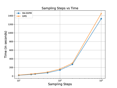
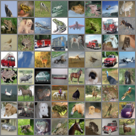
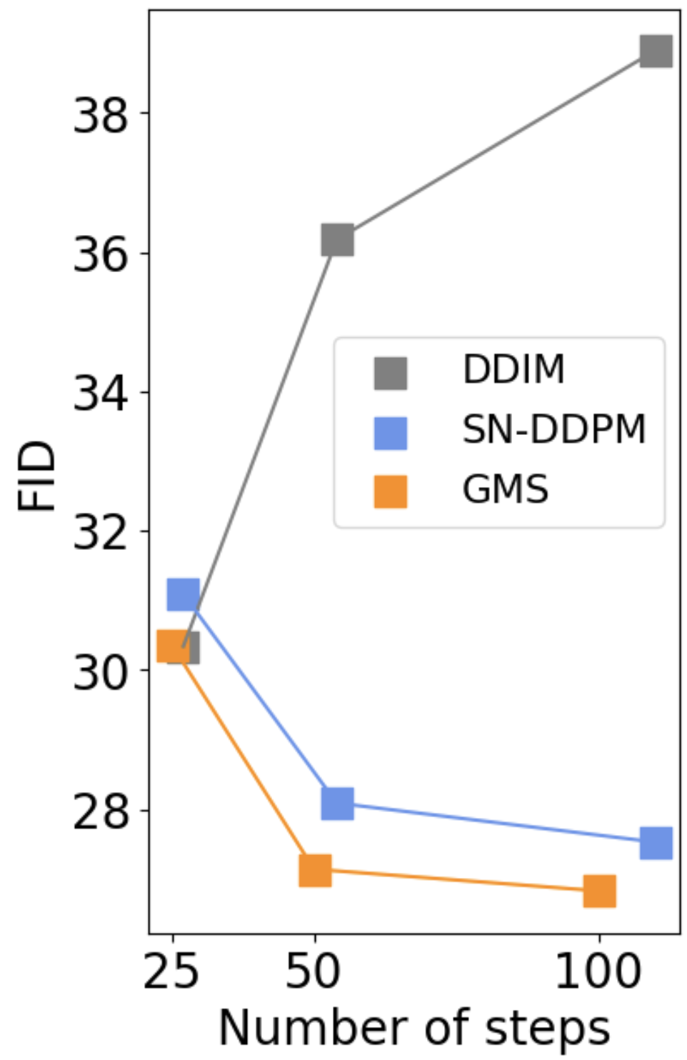
As shown in Tab. 1, GMS demonstrates superior performance compared to DDPM and SN-DDPM under the same number of steps in CIFAR10 and ImageNet 64 ×\times 64. Specifically, GMS achieves a remarkable 4.44 improvement in FID given 10 steps on CIFAR10. Appendix E.7 illustrates in more detail the improvement of GMS when the number of sampling steps is limited. Meanwhile, we conduct GMS in ImageNet 256 ×\times 256 via adopting the U-ViT-Huge [4] backbone as the noise network in Appendix E.8. Furthermore, taking into account the additional time required by GMS, our method still exhibits improved performance, as detailed in Appendix E.9. For integrity, we provide a comparison with other SDE-based solvers based on continuous time diffusion such as Gotta Go Fast [17], EDM [18] and SEED [10] in Appendix E.10 and shows that GMS largely outperforms other SDE-based solvers when the number of steps is less than 100. In Appendix G, we provide generated samples from GMS.

Table 1: Comparison with competitive SDE-based solvers w.r.t. FID score \downarrow on CIFAR10 and ImageNet 64×\times64. our GMS outperforms existing SDE-based solvers in most cases. SN-DDPM denotes Extended AnalyticDPM from Bao et al. [2].
CIFAR10 (LS)
# timesteps K𝐾K 10 20 25 40 50 100 200 1000
DDPM, β~tsubscript~𝛽𝑡\tilde{\beta}_{t} 43.14 25.28 21.63 15.24 15.21 10.94 8.23 5.11
DDPM, βtsubscript𝛽𝑡\beta_{t} 233.41 168.22 125.05 82.31 66.28 31.36 12.96 3.04
SN-DDPM 21.87 8.32 6.91 4.99 4.58 3.74 3.34 3.71
GMS (ours) 17.43 7.18 5.96 4.52 4.16 3.26 3.01 2.76
CIFAR10 (CS) ImageNet 64 ×\times 64
# timesteps K𝐾K 10 25 50 100 200 1000 25 50 100 200 400 4000
DDPM, β~tsubscript~𝛽𝑡\tilde{\beta}_{t} 34.76 16.18 11.11 8.38 6.66 4.92 29.21 21.71 19.12 17.81 17.48 16.55
DDPM, βtsubscript𝛽𝑡\beta_{t} 205.31 84.71 37.35 14.81 5.74 3.34 170.28 83.86 45.04 28.39 21.38 16.38
SN-DDPM 16.33 6.05 4.19 3.83 3.72 4.08 27.58 20.74 18.04 16.72 16.37 16.22
GMS (ours) 13.80 5.48 4.00 3.46 3.34 4.23 26.50 20.13 17.29 16.60 15.98 15.79

4.2 Stroke-based image synthesis based on SDEdit [27]

Evaluation metrics. We evaluate the editing results based on realism and faithfulness similar with Meng et al. [27]. To quantify the realism of sample images, we use FID between the generated images and the target realistic image dataset. To quantify faithfulness, we report the L2subscript𝐿2L_{2} distance summed over all pixels between the stroke images and the edited output images.

SDEdit [27] applies noise to the stroke image xgsuperscript𝑥𝑔x^{g} at time step t0subscript𝑡0t_{0} using 𝒩(xt0g|α(t)xg,σ2(t)I)𝒩conditionalsubscriptsuperscript𝑥𝑔subscript𝑡0𝛼𝑡superscript𝑥𝑔superscript𝜎2𝑡𝐼\mathcal{N}(x^{g}_{t_{0}}|\alpha(t)x^{g},\sigma^{2}(t)I) and discretize the reverse SDE in Eq. (4) for sampling. Fig. 9 demonstrates the significant impact of t0subscript𝑡0t_{0} on the realism of sampled images. As t0subscript𝑡0t_{0} increases, the similarity to real images decreases. we choose the range from t0=0.3Tsubscript𝑡00.3𝑇t_{0}=0.3T to t0=0.5Tsubscript𝑡00.5𝑇t_{0}=0.5T (T=1000𝑇1000T=1000 in our experiments) for our further experiments since sampled images closely resemble the real images in this range.
Refer to caption
(a) Trade-off between realism and faithfulness
Refer to caption
(b) t0=0.3Tsubscript𝑡00.3𝑇t_{0}=0.3T
Refer to caption
(c) t0=0.4Tsubscript𝑡00.4𝑇t_{0}=0.4T
Refer to caption
(d) t0=0.5Tsubscript𝑡00.5𝑇t_{0}=0.5T
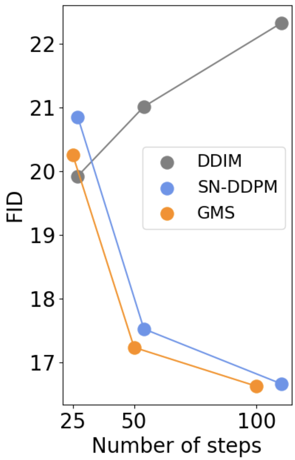
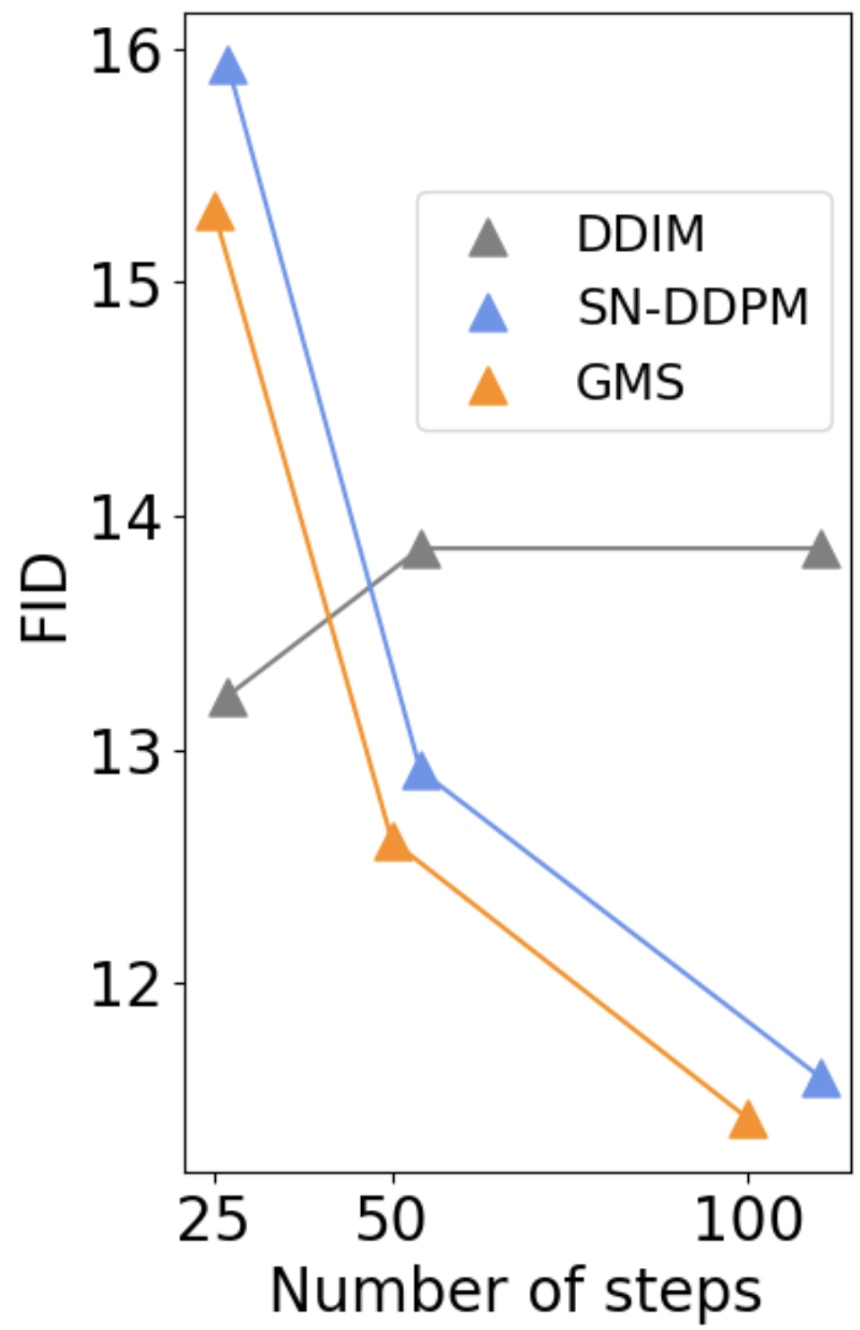
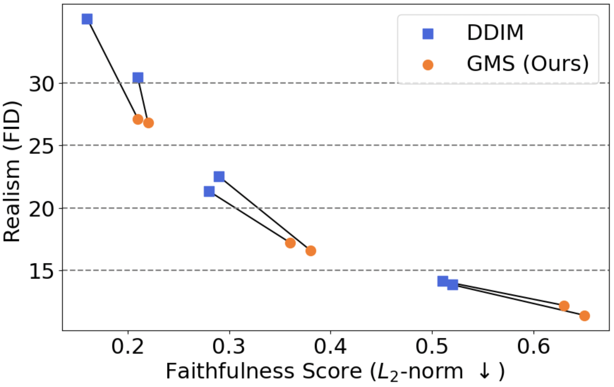
Figure 3: Result among different solvers in SDEdit. t0subscript𝑡0t_{0} denotes the time step of the start of reverse. (a): The points on each line represent the same t0subscript𝑡0t_{0} and the number of sampling steps. We select t0=[300,400,500]subscript𝑡0300400500t_{0}=[300,400,500], number of steps =[50,100]absent50100=[50,100]. (b): When t0=300subscript𝑡0300t_{0}=300, the effect of DDIM diminishes more prominently with the increase in the number of steps.

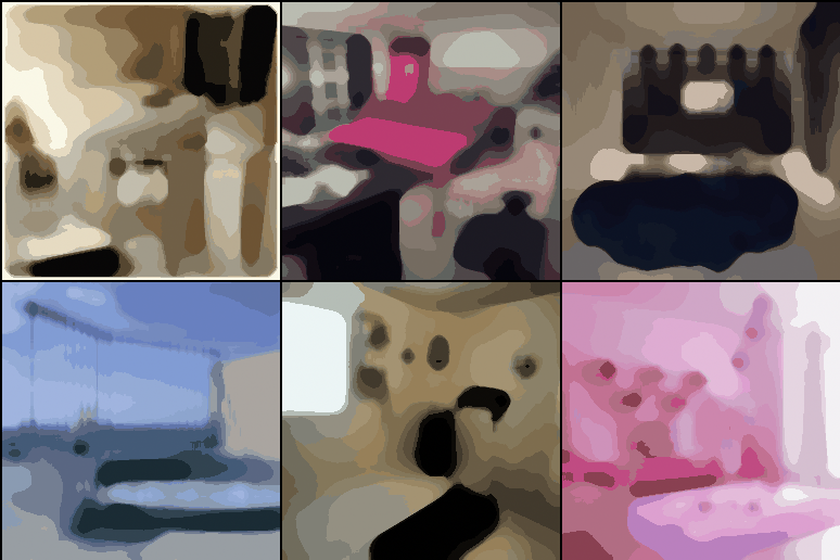
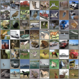
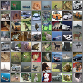
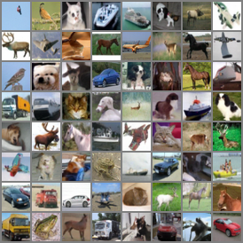
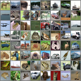
Fig. 3LABEL:sub@fig:compare illustrates that when using the same t0subscript𝑡0t_{0} and the same number of steps, edited output images from GMS have lower faithfulness but with higher realism. This phenomenon is likely attributed to the Gaussian noise introduced by the SDE-based solver during each sampling step. This noise causes the sampling to deviate from the original image (resulting in low faithfulness) but enables the solver to transition from the stroke domain to the real image domain. Fig. 3LABEL:sub@fig:sde1 to Fig. 3LABEL:sub@fig:sde3 further demonstrates this phenomenon to a certain extent. The realism of the sampled images generated by the SDE-based solver escalates with an increase in the number of sampling steps. Conversely, the realism of the sampled images produced by the ODE-based solver diminishes due to the absence of noise, which prevents the ODE-based solver from transitioning from the stroke domain to the real image domain. Additionally, in the SDEdit task, GMS exhibits superior performance compared to SN-DDPM [2] in terms of sample computation cost. Fig. 4 shows the samples using DDIM and GMS when t0=400subscript𝑡0400t_{0}=400 and the number of steps is 404040.

Refer to caption
(a) Real Images
Refer to caption
(b) Stroke
Refer to caption
(c) GMS
Refer to caption
(d) DDIM
Figure 4: SDEdit samples of GMS and DDIM. Due to the presence of noise, SDE-based solvers, such as GMS OURS, generate images with more details.

5 Related work

Faster solvers. In addition to SDE-based solvers, there are works dedicated to improving the efficiency of ODE-based solvers [25, 23, 8]. Some approaches use explicit reverse transition kernels, such as those based on generative adversarial networks proposed by Xiao et al. [40] and Wang et al. [39]. Gao et al. [9] employ an energy function to model the reverse transition kernel. Zhang and Chen [44] use a flow model for the transition kernel.

Non-Gaussian diffusion. Apart from diffusion, some literature suggests using non-Gaussian forward processes, which consequently involve non-Gaussian reverse processes. Bansal et al. [1] introduce a generalized noise operator that incorporates noise. Nachmani et al. [29] incorporate Gaussian mixture or Gamma noise into the forward process. While these works replace both the forward and reverse processes with non-Gaussian distributions, our approach aims to identify a suitable combination of non-Gaussian distributions to model the reverse process.

6 Conclusion

This paper presents a novel Gaussian mixture solver (GMS) for diffusion models. GMS relaxes the Gaussian reverse kernel assumption to reduce discretization errors and improves the sample quality under the same sampling steps. Experimental results show that GMS outperforms existing SDE-based solvers, achieving a remarkable 4.44 improvement in FID compared to the state-of-the-art SDE-based solver proposed by Bao et al. [2] given 10 steps. Furthermore, due to the presence of noise, SDE-based solvers prove more suitable for stroke-based synthesis tasks and GMS still outperforms state-of-the-art SDE-based solvers.

Limitations and broader impacts. While GMS enhances sample quality and potentially accelerates inference speed compared to existing SDE-based solvers, employing GMS still fall short of real-time applicability. Like other generative models, diffusion models can generate problematic fake content, and the use of GMS may amplify these undesirable effects.

Acknowledgement

This work was supported by NSF of China (Nos. 62076145); Beijing Outstanding Young Scientist Program (No. BJJWZYJH012019100020098); Major Innovation & Planning Interdisciplinary Platform for the “Double-First Class” Initiative, Renmin University of China; the Fundamental Research Funds for the Central Universities, and the Research Funds of Renmin University of China (No. 22XNKJ13). C. Li was also sponsored by Beijing Nova Program (No. 20220484044).

References

  • Bansal et al. [2022] Arpit Bansal, Eitan Borgnia, Hong-Min Chu, Jie S Li, Hamid Kazemi, Furong Huang, Micah Goldblum, Jonas Geiping, and Tom Goldstein. Cold diffusion: Inverting arbitrary image transforms without noise. arXiv preprint arXiv:2208.09392, 2022.
  • Bao et al. [2022a] Fan Bao, Chongxuan Li, Jiacheng Sun, Jun Zhu, and Bo Zhang. Estimating the optimal covariance with imperfect mean in diffusion probabilistic models. arXiv preprint arXiv:2206.07309, 2022a.
  • Bao et al. [2022b] Fan Bao, Chongxuan Li, Jun Zhu, and Bo Zhang. Analytic-dpm: an analytic estimate of the optimal reverse variance in diffusion probabilistic models. arXiv preprint arXiv:2201.06503, 2022b.
  • Bao et al. [2023a] Fan Bao, Shen Nie, Kaiwen Xue, Yue Cao, Chongxuan Li, Hang Su, and Jun Zhu. All are worth words: A vit backbone for diffusion models. In Proceedings of the IEEE/CVF Conference on Computer Vision and Pattern Recognition, pages 22669–22679, 2023a.
  • Bao et al. [2023b] Fan Bao, Shen Nie, Kaiwen Xue, Chongxuan Li, Shi Pu, Yaole Wang, Gang Yue, Yue Cao, Hang Su, and Jun Zhu. One transformer fits all distributions in multi-modal diffusion at scale. arXiv preprint arXiv:2303.06555, 2023b.
  • Chen et al. [2020] Xinlei Chen, Haoqi Fan, Ross Girshick, and Kaiming He. Improved baselines with momentum contrastive learning. arXiv preprint arXiv:2003.04297, 2020.
  • Dhariwal and Nichol [2021] Prafulla Dhariwal and Alexander Nichol. Diffusion models beat gans on image synthesis. Advances in Neural Information Processing Systems, 34:8780–8794, 2021.
  • Dockhorn et al. [2022] Tim Dockhorn, Arash Vahdat, and Karsten Kreis. Genie: Higher-order denoising diffusion solvers. arXiv preprint arXiv:2210.05475, 2022.
  • Gao et al. [2020] Ruiqi Gao, Yang Song, Ben Poole, Ying Nian Wu, and Diederik P Kingma. Learning energy-based models by diffusion recovery likelihood. arXiv preprint arXiv:2012.08125, 2020.
  • Gonzalez et al. [2023] Martin Gonzalez, Nelson Fernandez, Thuy Tran, Elies Gherbi, Hatem Hajri, and Nader Masmoudi. Seeds: Exponential sde solvers for fast high-quality sampling from diffusion models. arXiv preprint arXiv:2305.14267, 2023.
  • Hansen [1982] Lars Peter Hansen. Large sample properties of generalized method of moments estimators. Econometrica: Journal of the econometric society, pages 1029–1054, 1982.
  • Hertz et al. [2022] Amir Hertz, Ron Mokady, Jay Tenenbaum, Kfir Aberman, Yael Pritch, and Daniel Cohen-Or. Prompt-to-prompt image editing with cross attention control. arXiv preprint arXiv:2208.01626, 2022.
  • Heusel et al. [2017] Martin Heusel, Hubert Ramsauer, Thomas Unterthiner, Bernhard Nessler, and Sepp Hochreiter. Gans trained by a two time-scale update rule converge to a local nash equilibrium. Advances in neural information processing systems, 30, 2017.
  • Ho et al. [2020] Jonathan Ho, Ajay Jain, and Pieter Abbeel. Denoising diffusion probabilistic models. Advances in Neural Information Processing Systems, 33:6840–6851, 2020.
  • Ho et al. [2022a] Jonathan Ho, Chitwan Saharia, William Chan, David J Fleet, Mohammad Norouzi, and Tim Salimans. Cascaded diffusion models for high fidelity image generation. J. Mach. Learn. Res., 23(47):1–33, 2022a.
  • Ho et al. [2022b] Jonathan Ho, Tim Salimans, Alexey Gritsenko, William Chan, Mohammad Norouzi, and David J Fleet. Video diffusion models. arXiv preprint arXiv:2204.03458, 2022b.
  • Jolicoeur-Martineau et al. [2021] Alexia Jolicoeur-Martineau, Ke Li, Rémi Piché-Taillefer, Tal Kachman, and Ioannis Mitliagkas. Gotta go fast when generating data with score-based models. arXiv preprint arXiv:2105.14080, 2021.
  • Karras et al. [2022] Tero Karras, Miika Aittala, Timo Aila, and Samuli Laine. Elucidating the design space of diffusion-based generative models. arXiv preprint arXiv:2206.00364, 2022.
  • Kawar et al. [2022a] Bahjat Kawar, Michael Elad, Stefano Ermon, and Jiaming Song. Denoising diffusion restoration models. arXiv preprint arXiv:2201.11793, 2022a.
  • Kawar et al. [2022b] Bahjat Kawar, Shiran Zada, Oran Lang, Omer Tov, Huiwen Chang, Tali Dekel, Inbar Mosseri, and Michal Irani. Imagic: Text-based real image editing with diffusion models. arXiv preprint arXiv:2210.09276, 2022b.
  • Kingma et al. [2021] Diederik Kingma, Tim Salimans, Ben Poole, and Jonathan Ho. Variational diffusion models. Advances in neural information processing systems, 34:21696–21707, 2021.
  • Kong et al. [2020] Zhifeng Kong, Wei Ping, Jiaji Huang, Kexin Zhao, and Bryan Catanzaro. Diffwave: A versatile diffusion model for audio synthesis. arXiv preprint arXiv:2009.09761, 2020.
  • Liu et al. [2022] Luping Liu, Yi Ren, Zhijie Lin, and Zhou Zhao. Pseudo numerical methods for diffusion models on manifolds. arXiv preprint arXiv:2202.09778, 2022.
  • Lu [2023] Cheng Lu, 2023. https://github.com/huggingface/diffusers/pull/3344.
  • Lu et al. [2022] Cheng Lu, Yuhao Zhou, Fan Bao, Jianfei Chen, Chongxuan Li, and Jun Zhu. Dpm-solver: A fast ode solver for diffusion probabilistic model sampling in around 10 steps. arXiv preprint arXiv:2206.00927, 2022.
  • McLachlan and Krishnan [2007] Geoffrey J McLachlan and Thriyambakam Krishnan. The EM algorithm and extensions. John Wiley & Sons, 2007.
  • Meng et al. [2021] Chenlin Meng, Yang Song, Jiaming Song, Jiajun Wu, Jun-Yan Zhu, and Stefano Ermon. Sdedit: Image synthesis and editing with stochastic differential equations. arXiv preprint arXiv:2108.01073, 2021.
  • Nachmani and Dovrat [2021] Eliya Nachmani and Shaked Dovrat. Zero-shot translation using diffusion models. arXiv preprint arXiv:2111.01471, 2021.
  • Nachmani et al. [2021] Eliya Nachmani, Robin San Roman, and Lior Wolf. Non gaussian denoising diffusion models. arXiv preprint arXiv:2106.07582, 2021.
  • Nichol and Dhariwal [2021] Alexander Quinn Nichol and Prafulla Dhariwal. Improved denoising diffusion probabilistic models. In International Conference on Machine Learning, pages 8162–8171. PMLR, 2021.
  • Poole et al. [2022] Ben Poole, Ajay Jain, Jonathan T Barron, and Ben Mildenhall. Dreamfusion: Text-to-3d using 2d diffusion. arXiv preprint arXiv:2209.14988, 2022.
  • Popov et al. [2021] Vadim Popov, Ivan Vovk, Vladimir Gogoryan, Tasnima Sadekova, and Mikhail Kudinov. Grad-tts: A diffusion probabilistic model for text-to-speech. In International Conference on Machine Learning, pages 8599–8608. PMLR, 2021.
  • Ramachandran et al. [2017] Prajit Ramachandran, Barret Zoph, and Quoc V Le. Searching for activation functions. arXiv preprint arXiv:1710.05941, 2017.
  • Shonenkov et al. [2023] Alex Shonenkov, Misha Konstantinov, Daria Bakshandaeva, Christoph Schuhmann, Ksenia Ivanova, and Nadiia Klokova, 2023. https://github.com/deep-floyd/IF.
  • Sohl-Dickstein et al. [2015] Jascha Sohl-Dickstein, Eric Weiss, Niru Maheswaranathan, and Surya Ganguli. Deep unsupervised learning using nonequilibrium thermodynamics. In International Conference on Machine Learning, pages 2256–2265. PMLR, 2015.
  • Song et al. [2020a] Jiaming Song, Chenlin Meng, and Stefano Ermon. Denoising diffusion implicit models. arXiv preprint arXiv:2010.02502, 2020a.
  • Song et al. [2020b] Yang Song, Jascha Sohl-Dickstein, Diederik P Kingma, Abhishek Kumar, Stefano Ermon, and Ben Poole. Score-based generative modeling through stochastic differential equations. arXiv preprint arXiv:2011.13456, 2020b.
  • Vincent [2011] Pascal Vincent. A connection between score matching and denoising autoencoders. Neural computation, 23(7):1661–1674, 2011.
  • Wang et al. [2022] Zhendong Wang, Huangjie Zheng, Pengcheng He, Weizhu Chen, and Mingyuan Zhou. Diffusion-gan: Training gans with diffusion. arXiv preprint arXiv:2206.02262, 2022.
  • Xiao et al. [2021] Zhisheng Xiao, Karsten Kreis, and Arash Vahdat. Tackling the generative learning trilemma with denoising diffusion gans. arXiv preprint arXiv:2112.07804, 2021.
  • Xie et al. [2022] Xingyu Xie, Pan Zhou, Huan Li, Zhouchen Lin, and Shuicheng Yan. Adan: Adaptive nesterov momentum algorithm for faster optimizing deep models. arXiv preprint arXiv:2208.06677, 2022.
  • Xu et al. [2022] Xingqian Xu, Zhangyang Wang, Eric Zhang, Kai Wang, and Humphrey Shi. Versatile diffusion: Text, images and variations all in one diffusion model. arXiv preprint arXiv:2211.08332, 2022.
  • Zhang and Agrawala [2023] Lvmin Zhang and Maneesh Agrawala. Adding conditional control to text-to-image diffusion models. arXiv preprint arXiv:2302.05543, 2023.
  • Zhang and Chen [2021] Qinsheng Zhang and Yongxin Chen. Diffusion normalizing flow. Advances in Neural Information Processing Systems, 34:16280–16291, 2021.
  • Zhao et al. [2022] Min Zhao, Fan Bao, Chongxuan Li, and Jun Zhu. Egsde: Unpaired image-to-image translation via energy-guided stochastic differential equations. arXiv preprint arXiv:2207.06635, 2022.

Appendix A Proof

A.1 Proof of Proposition 3.1

When q(x0)𝑞subscript𝑥0q(x_{0}) is a mixture of Dirac distribution which means that q(x0)=i=1Mwiδ(xxi),i=1Mwi=1formulae-sequence𝑞subscript𝑥0superscriptsubscript𝑖1𝑀subscript𝑤𝑖𝛿𝑥subscript𝑥𝑖superscriptsubscript𝑖1𝑀subscript𝑤𝑖1q(x_{0})=\sum_{i=1}^{M}w_{i}\delta(x-x_{i}),\sum_{i=1}^{M}w_{i}=1, which has total M𝑀M components, and when the forward process q(xt|x0)𝑞conditionalsubscript𝑥𝑡subscript𝑥0q(x_{t}|x_{0}) is a Gaussian distribution as Eq. (1), the reverse process q(xs|xt)𝑞conditionalsubscript𝑥𝑠subscript𝑥𝑡q(x_{s}|x_{t}) would be:

q(xs|xt)=q(xs|xt,x0)q(x0|xt)𝑑x0=q(xs|xt,x0)q(x0)q(xt|x0)/q(xt)𝑑x0𝑞conditionalsubscript𝑥𝑠subscript𝑥𝑡𝑞conditionalsubscript𝑥𝑠subscript𝑥𝑡subscript𝑥0𝑞conditionalsubscript𝑥0subscript𝑥𝑡differential-dsubscript𝑥0𝑞conditionalsubscript𝑥𝑠subscript𝑥𝑡subscript𝑥0𝑞subscript𝑥0𝑞conditionalsubscript𝑥𝑡subscript𝑥0𝑞subscript𝑥𝑡differential-dsubscript𝑥0\displaystyle q(x_{s}|x_{t})=\int q(x_{s}|x_{t},x_{0})q(x_{0}|x_{t})dx_{0}=\int q(x_{s}|x_{t},x_{0})q(x_{0})q(x_{t}|x_{0})/q(x_{t})dx_{0}
=1/q(xt)q(xs|xt,x0)q(x0)q(xt|x0)𝑑x0=1/q(xt)i=1Mwiq(xs|xt,x0i)q(xt|x0i)absent1𝑞subscript𝑥𝑡𝑞conditionalsubscript𝑥𝑠subscript𝑥𝑡subscript𝑥0𝑞subscript𝑥0𝑞conditionalsubscript𝑥𝑡subscript𝑥0differential-dsubscript𝑥01𝑞subscript𝑥𝑡superscriptsubscript𝑖1𝑀subscript𝑤𝑖𝑞conditionalsubscript𝑥𝑠subscript𝑥𝑡superscriptsubscript𝑥0𝑖𝑞conditionalsubscript𝑥𝑡superscriptsubscript𝑥0𝑖\displaystyle=1/q(x_{t})\int q(x_{s}|x_{t},x_{0})q(x_{0})q(x_{t}|x_{0})dx_{0}=1/q(x_{t})\sum_{i=1}^{M}w_{i}q(x_{s}|x_{t},x_{0}^{i})q(x_{t}|x_{0}^{i})

According to the definition of forward process, the distribution q(xt|x0i)=𝒩(xt|a¯tx0i,(1a¯t)I)𝑞conditionalsubscript𝑥𝑡superscriptsubscript𝑥0𝑖𝒩conditionalsubscript𝑥𝑡subscript¯𝑎𝑡superscriptsubscript𝑥0𝑖1subscript¯𝑎𝑡𝐼q(x_{t}|x_{0}^{i})=\mathcal{N}(x_{t}|\sqrt{\bar{a}_{t}}x_{0}^{i},(1-\bar{a}_{t})I). Due to the Markov property of forward process, when t>s𝑡𝑠t>s, we have q(xs,xt|x0)q(xs|x0)q(xt|xs)𝑞subscript𝑥𝑠conditionalsubscript𝑥𝑡subscript𝑥0𝑞conditionalsubscript𝑥𝑠subscript𝑥0𝑞conditionalsubscript𝑥𝑡subscript𝑥𝑠q(x_{s},x_{t}|x_{0})q(x_{s}|x_{0})q(x_{t}|x_{s}). The term q(xs|xt,x0)𝑞conditionalsubscript𝑥𝑠subscript𝑥𝑡subscript𝑥0q(x_{s}|x_{t},x_{0}) would be viewed as a Bayesian posterior resulting from a prior q(xs|x0)𝑞conditionalsubscript𝑥𝑠subscript𝑥0q(x_{s}|x_{0}), updated with a likelihood term q(xt|xs)𝑞conditionalsubscript𝑥𝑡subscript𝑥𝑠q(x_{t}|x_{s}). And therefore

q(xs|xt,x0i)=N(xs|μq(xt,x0),Σq(xt,x0)I)=𝒩(xs|at|sσs2σt2xt+asσt|s2σt2x0,σs2σt|s2σt2I)𝑞conditionalsubscript𝑥𝑠subscript𝑥𝑡superscriptsubscript𝑥0𝑖𝑁conditionalsubscript𝑥𝑠subscript𝜇𝑞subscript𝑥𝑡subscript𝑥0subscriptΣ𝑞subscript𝑥𝑡subscript𝑥0𝐼𝒩conditionalsubscript𝑥𝑠subscript𝑎conditional𝑡𝑠subscriptsuperscript𝜎2𝑠subscriptsuperscript𝜎2𝑡subscript𝑥𝑡subscript𝑎𝑠superscriptsubscript𝜎conditional𝑡𝑠2subscriptsuperscript𝜎2𝑡subscript𝑥0subscriptsuperscript𝜎2𝑠superscriptsubscript𝜎conditional𝑡𝑠2subscriptsuperscript𝜎2𝑡𝐼\displaystyle q(x_{s}|x_{t},x_{0}^{i})=N(x_{s}|\mu_{q}(x_{t},x_{0}),\Sigma_{q}(x_{t},x_{0})I)=\mathcal{N}(x_{s}|\frac{a_{t|s}\sigma^{2}_{s}}{\sigma^{2}_{t}}x_{t}+\frac{a_{s}\sigma_{t|s}^{2}}{\sigma^{2}_{t}}x_{0},\frac{\sigma^{2}_{s}\sigma_{t|s}^{2}}{\sigma^{2}_{t}}I)

It is easy to prove that, the distribution q(xs|xt)𝑞conditionalsubscript𝑥𝑠subscript𝑥𝑡q(x_{s}|x_{t}) is a mixture of Gaussian distribution:

q(xs|xt)i=1Mwiq(xs|xt,x0i)q(xt|x0i)proportional-to𝑞conditionalsubscript𝑥𝑠subscript𝑥𝑡superscriptsubscript𝑖1𝑀subscript𝑤𝑖𝑞conditionalsubscript𝑥𝑠subscript𝑥𝑡superscriptsubscript𝑥0𝑖𝑞conditionalsubscript𝑥𝑡superscriptsubscript𝑥0𝑖\displaystyle q(x_{s}|x_{t})\propto\sum_{i=1}^{M}w_{i}q(x_{s}|x_{t},x_{0}^{i})q(x_{t}|x_{0}^{i})
=i=1Mwi𝒩(xt|a¯tx0i,(1at¯)I)𝒩(xs|μq(xt,x0),Σq(xt,x0))absentsuperscriptsubscript𝑖1𝑀subscript𝑤𝑖𝒩conditionalsubscript𝑥𝑡subscript¯𝑎𝑡superscriptsubscript𝑥0𝑖1¯subscript𝑎𝑡𝐼𝒩conditionalsubscript𝑥𝑠subscript𝜇𝑞subscript𝑥𝑡subscript𝑥0subscriptΣ𝑞subscript𝑥𝑡subscript𝑥0\displaystyle=\sum_{i=1}^{M}w_{i}\mathcal{N}(x_{t}|\sqrt{\bar{a}_{t}}x_{0}^{i},(1-\bar{a_{t}})I)*\mathcal{N}(x_{s}|\mu_{q}(x_{t},x_{0}),\Sigma_{q}(x_{t},x_{0}))

When t𝑡t is large, s𝑠s is small, σt|s2superscriptsubscript𝜎conditional𝑡𝑠2\sigma_{t|s}^{2} would be large, meaning that the influence of x0isuperscriptsubscript𝑥0𝑖x_{0}^{i} would be large.

Secondly, when q(x0)𝑞subscript𝑥0q(x_{0}) is a mixture of Gaussian distribution which means that q(x0)=i=1Mwi𝒩(x0i|μi,Σi),i=1Mwi=1formulae-sequence𝑞subscript𝑥0superscriptsubscript𝑖1𝑀subscript𝑤𝑖𝒩conditionalsuperscriptsubscript𝑥0𝑖subscript𝜇𝑖subscriptΣ𝑖superscriptsubscript𝑖1𝑀subscript𝑤𝑖1q(x_{0})=\sum_{i=1}^{M}w_{i}\mathcal{N}(x_{0}^{i}|\mu_{i},\Sigma_{i}),\sum_{i=1}^{M}w_{i}=1. For simplicity of analysis, we assume that this distribution is a one-dimensional distribution or that the covariance matrix is a high-dimensional Gaussian distribution with a diagonal matrix Σi=diagi(σ2)subscriptΣ𝑖subscriptdiag𝑖superscript𝜎2\Sigma_{i}=\textrm{diag}_{i}(\sigma^{2}). Similar to the situation above, for each dimension in the reverse process:

q(xs|xt)=1/q(xt)q(xs|xt,x0)q(x0)q(xt|x0)𝑑x0𝑞conditionalsubscript𝑥𝑠subscript𝑥𝑡1𝑞subscript𝑥𝑡𝑞conditionalsubscript𝑥𝑠subscript𝑥𝑡subscript𝑥0𝑞subscript𝑥0𝑞conditionalsubscript𝑥𝑡subscript𝑥0differential-dsubscript𝑥0\displaystyle q(x_{s}|x_{t})=1/q(x_{t})\int q(x_{s}|x_{t},x_{0})q(x_{0})q(x_{t}|x_{0})dx_{0}
=i=1Mwi/q(xt)q(xs|xt,x0)𝒩(x0|μi,Σi)q(xt|x0)𝑑x0absentsuperscriptsubscript𝑖1𝑀subscript𝑤𝑖𝑞subscript𝑥𝑡𝑞conditionalsubscript𝑥𝑠subscript𝑥𝑡subscript𝑥0𝒩conditionalsubscript𝑥0subscript𝜇𝑖subscriptΣ𝑖𝑞conditionalsubscript𝑥𝑡subscript𝑥0differential-dsubscript𝑥0\displaystyle=\sum_{i=1}^{M}w_{i}/q(x_{t})\int q(x_{s}|x_{t},x_{0})\mathcal{N}(x_{0}|\mu_{i},\Sigma_{i})q(x_{t}|x_{0})dx_{0}
=i=1Mwi/q(xt)12πσqe(x0iμq)2σq212πσie(x0iμi)2σi212π1a¯te(xta¯tx0)21a¯t𝑑x0absentsuperscriptsubscript𝑖1𝑀subscript𝑤𝑖𝑞subscript𝑥𝑡12𝜋subscript𝜎𝑞superscript𝑒superscriptsuperscriptsubscript𝑥0𝑖subscript𝜇𝑞2superscriptsubscript𝜎𝑞212𝜋subscript𝜎𝑖superscript𝑒superscriptsuperscriptsubscript𝑥0𝑖subscript𝜇𝑖2superscriptsubscript𝜎𝑖212𝜋1subscript¯𝑎𝑡superscript𝑒superscriptsubscript𝑥𝑡subscript¯𝑎𝑡subscript𝑥021subscript¯𝑎𝑡differential-dsubscript𝑥0\displaystyle=\sum_{i=1}^{M}w_{i}/q(x_{t})\int\frac{1}{\sqrt{2\pi}\sigma_{q}}e^{-\frac{(x_{0}^{i}-\mu_{q})^{2}}{\sigma_{q}^{2}}}\frac{1}{\sqrt{2\pi}\sigma_{i}}e^{-\frac{(x_{0}^{i}-\mu_{i})^{2}}{\sigma_{i}^{2}}}\frac{1}{\sqrt{2\pi}\sqrt{1-\bar{a}_{t}}}e^{-\frac{(x_{t}-\sqrt{\bar{a}_{t}x_{0}})^{2}}{1-\bar{a}_{t}}}dx_{0}
=i=1Mwi/q(xt)Zi12πσxe(x0iμx)2σx2e(xsμ(xt))2σ(xt)𝑑x0absentsuperscriptsubscript𝑖1𝑀subscript𝑤𝑖𝑞subscript𝑥𝑡subscript𝑍𝑖12𝜋subscript𝜎𝑥superscript𝑒superscriptsuperscriptsubscript𝑥0𝑖subscript𝜇𝑥2superscriptsubscript𝜎𝑥2superscript𝑒superscriptsubscript𝑥𝑠𝜇subscript𝑥𝑡2𝜎subscript𝑥𝑡differential-dsubscript𝑥0\displaystyle=\sum_{i=1}^{M}w_{i}/q(x_{t})\int Z_{i}\frac{1}{\sqrt{2\pi}\sigma_{x}}e^{-\frac{(x_{0}^{i}-\mu_{x})^{2}}{\sigma_{x}^{2}}}e^{-\frac{(x_{s}-\mu(x_{t}))^{2}}{\sigma(x_{t})}}dx_{0}

And q(xs|xt)𝑞conditionalsubscript𝑥𝑠subscript𝑥𝑡q(x_{s}|x_{t}) could be a Gaussian mixture which has M𝑀M component.

A.2 Proof of Proposition 3.2

Recall that our objective function is to find optimal parameters:

θ^=argmin𝜃[QNc(θ)1×1]=argmin𝜃[gNc(θ)T1×NWNcN×NgNc(θ)1×N]^𝜃𝜃argmindelimited-[]subscriptsubscript𝑄subscript𝑁𝑐𝜃11𝜃argmindelimited-[]subscriptsubscript𝑔subscript𝑁𝑐superscript𝜃𝑇1𝑁subscriptsubscript𝑊subscript𝑁𝑐𝑁𝑁subscriptsubscript𝑔subscript𝑁𝑐𝜃1𝑁\displaystyle\hat{\theta}=\underset{\theta}{\textrm{argmin}}[{\underbrace{Q_{N_{c}}(\theta)}_{1\times 1}}]=\underset{\theta}{\textrm{argmin}}[{\underbrace{g_{N_{c}}(\theta)^{T}}_{1\times N}}{\underbrace{W_{N_{c}}}_{N\times N}}{\underbrace{g_{N_{c}}(\theta)}_{1\times N}}] (14)

where gM(θ)subscript𝑔𝑀𝜃g_{M}(\theta) is the moment conditions talked about in Sec. 3.2, W𝑊W is the weighted Matrix, Ncsubscript𝑁𝑐{N_{c}} is the sample size. When solving such problems using optimizers, which are equivalent to the one we used when selecting θGMMsubscript𝜃𝐺𝑀𝑀\theta_{GMM} such that QT(θGMM)θ=0subscript𝑄𝑇subscript𝜃𝐺𝑀𝑀𝜃0\frac{\partial Q_{T}(\theta_{GMM})}{\partial\theta}=0, and its first derivative:

QNc(θ)θd×1=(QNc(θ)θ1QNc(θ)θ2QNc(θ)θ3),QNc(θ)θm=2[1Nci=1Ncg(xi,θ)θm]T1×NWNcN×N[1Nci=1Mg(xi,θ)]N×1formulae-sequencesubscriptsubscript𝑄subscript𝑁𝑐𝜃𝜃𝑑1matrixsubscript𝑄subscript𝑁𝑐𝜃subscript𝜃1subscript𝑄subscript𝑁𝑐𝜃subscript𝜃2subscript𝑄subscript𝑁𝑐𝜃subscript𝜃3subscript𝑄subscript𝑁𝑐𝜃subscript𝜃𝑚2subscriptsuperscriptdelimited-[]1subscript𝑁𝑐superscriptsubscript𝑖1subscript𝑁𝑐𝑔subscript𝑥𝑖𝜃subscript𝜃𝑚𝑇1𝑁subscriptsubscript𝑊subscript𝑁𝑐𝑁𝑁subscriptdelimited-[]1subscript𝑁𝑐superscriptsubscript𝑖1𝑀𝑔subscript𝑥𝑖𝜃𝑁1\displaystyle\underbrace{\frac{\partial Q_{N_{c}}(\theta)}{\partial\theta}}_{d\times 1}=\begin{pmatrix}\frac{\partial Q_{N_{c}}(\theta)}{\partial\theta_{1}}\\ \frac{\partial Q_{N_{c}}(\theta)}{\partial\theta_{2}}\\ \frac{\partial Q_{N_{c}}(\theta)}{\partial\theta_{3}}\end{pmatrix},\frac{\partial Q_{N_{c}}(\theta)}{\partial\theta_{m}}=2\underbrace{[\frac{1}{{N_{c}}}\sum_{i=1}^{{N_{c}}}\frac{\partial g(x_{i},\theta)}{\partial\theta_{m}}]^{T}}_{1\times N}\underbrace{W_{N_{c}}}_{N\times N}\underbrace{[\frac{1}{{N_{c}}}\sum_{i=1}^{M}g(x_{i},\theta)]}_{N\times 1} (15)

its second derivative (the Hessian matrix):

2QNc(θ)θ2d×dsubscriptsuperscript2subscript𝑄subscript𝑁𝑐𝜃superscript𝜃2𝑑𝑑\displaystyle\underbrace{\frac{\partial^{2}Q_{N_{c}}(\theta)}{\partial\theta^{2}}}_{d\times d} =(2QNc(θ)θ1θ12QNc(θ)θ1θ22QNc(θ)θ1θd2QNc(θ)θ2θ12QNc(θ)θdθd)absentmatrixsuperscript2subscript𝑄subscript𝑁𝑐𝜃subscript𝜃1subscript𝜃1superscript2subscript𝑄subscript𝑁𝑐𝜃subscript𝜃1subscript𝜃2superscript2subscript𝑄subscript𝑁𝑐𝜃subscript𝜃1subscript𝜃𝑑superscript2subscript𝑄subscript𝑁𝑐𝜃subscript𝜃2subscript𝜃1superscript2subscript𝑄subscript𝑁𝑐𝜃subscript𝜃𝑑subscript𝜃𝑑\displaystyle=\begin{pmatrix}\frac{\partial^{2}Q_{N_{c}}(\theta)}{\partial\theta_{1}\theta_{1}}&\frac{\partial^{2}Q_{N_{c}}(\theta)}{\partial\theta_{1}\theta_{2}}&...&\frac{\partial^{2}Q_{N_{c}}(\theta)}{\partial\theta_{1}\theta_{d}}\\ \frac{\partial^{2}Q_{N_{c}}(\theta)}{\partial\theta_{2}\theta_{1}}&...&...&...\\ ...&...&...&...\\ ...&...&...&\frac{\partial^{2}Q_{N_{c}}(\theta)}{\partial\theta_{d}\theta_{d}}\end{pmatrix} (16)
,2QNc(θ)θiθj\displaystyle,\frac{\partial^{2}Q_{N_{c}}(\theta)}{\partial\theta_{i}\theta_{j}} =2[1Mi=1Ncg(xi,θ)θi]TWNc[1Nci=1Ncg(xi,θ)θj]absent2superscriptdelimited-[]1𝑀superscriptsubscript𝑖1subscript𝑁𝑐𝑔subscript𝑥𝑖𝜃subscript𝜃𝑖𝑇subscript𝑊subscript𝑁𝑐delimited-[]1subscript𝑁𝑐superscriptsubscript𝑖1subscript𝑁𝑐𝑔subscript𝑥𝑖𝜃subscript𝜃𝑗\displaystyle=2[\frac{1}{M}\sum_{i=1}^{N_{c}}\frac{\partial g(x_{i},\theta)}{\partial\theta_{i}}]^{T}W_{N_{c}}[\frac{1}{N_{c}}\sum_{i=1}^{N_{c}}\frac{\partial g(x_{i},\theta)}{\partial\theta_{j}}]
+2[1Nci=1Nc2g(xi,θ)θiθj]WNc[1Nci=1Ncg(xi,θ)].2delimited-[]1subscript𝑁𝑐superscriptsubscript𝑖1subscript𝑁𝑐superscript2𝑔subscript𝑥𝑖𝜃subscript𝜃𝑖subscript𝜃𝑗subscript𝑊subscript𝑁𝑐delimited-[]1subscript𝑁𝑐superscriptsubscript𝑖1subscript𝑁𝑐𝑔subscript𝑥𝑖𝜃\displaystyle+2[\frac{1}{N_{c}}\sum_{i=1}^{N_{c}}\frac{\partial^{2}g(x_{i},\theta)}{\partial\theta_{i}\theta_{j}}]W_{N_{c}}[\frac{1}{N_{c}}\sum_{i=1}^{N_{c}}g(x_{i},\theta)].

By Taylor’s expansion of the gradient around optimal parameters θ0subscript𝜃0\theta_{0}, we have:

QNc(θGMM)θQNc(θ0)θ2QNc(θ0)θθT(θGMMθ)subscript𝑄subscript𝑁𝑐subscript𝜃𝐺𝑀𝑀𝜃subscript𝑄subscript𝑁𝑐subscript𝜃0𝜃superscript2subscript𝑄subscript𝑁𝑐subscript𝜃0𝜃superscript𝜃𝑇subscript𝜃𝐺𝑀𝑀𝜃\displaystyle\frac{\partial Q_{N_{c}}(\theta_{GMM})}{\partial\theta}-\frac{\partial Q_{N_{c}}(\theta_{0})}{\partial\theta}\approx\frac{\partial^{2}Q_{N_{c}}(\theta_{0})}{\partial\theta\partial\theta^{T}}(\theta_{GMM}-\theta) (17)
(θGMMθ)(2QNc(θ0)θθT)1QNc(θ0)θ.absentsubscript𝜃𝐺𝑀𝑀𝜃superscriptsuperscript2subscript𝑄subscript𝑁𝑐subscript𝜃0𝜃superscript𝜃𝑇1subscript𝑄subscript𝑁𝑐subscript𝜃0𝜃\displaystyle\longmapsto(\theta_{GMM}-\theta)\approx-(\frac{\partial^{2}Q_{N_{c}}(\theta_{0})}{\partial\theta\partial\theta^{T}})^{-1}\frac{\partial Q_{N_{c}}(\theta_{0})}{\partial\theta}.

Consider one element of the gradient vector QNc(θ0)θmsubscript𝑄subscript𝑁𝑐subscript𝜃0subscript𝜃𝑚\frac{\partial Q_{N_{c}}(\theta_{0})}{\partial\theta_{m}}

QNc(θ0)θm=2[1Mi=1Ncg(xi,θ0)θm𝑝𝔼(g(xi,θ0)θm)=Γ0,m]TWNc𝑝W[1Nci=1Ncg(xi,θ0)𝑝𝔼[g(xi,θ0)]=0].subscript𝑄subscript𝑁𝑐subscript𝜃0subscript𝜃𝑚2superscriptdelimited-[]subscript1𝑀superscriptsubscript𝑖1subscript𝑁𝑐𝑔subscript𝑥𝑖subscript𝜃0subscript𝜃𝑚𝑝𝔼𝑔subscript𝑥𝑖subscript𝜃0subscript𝜃𝑚subscriptΓ0𝑚𝑇subscriptsubscript𝑊subscript𝑁𝑐𝑝𝑊delimited-[]subscript1subscript𝑁𝑐superscriptsubscript𝑖1subscript𝑁𝑐𝑔subscript𝑥𝑖subscript𝜃0𝑝𝔼delimited-[]𝑔subscript𝑥𝑖subscript𝜃00\displaystyle\frac{\partial Q_{N_{c}}(\theta_{0})}{\partial\theta_{m}}=2[\underbrace{\frac{1}{M}\sum_{i=1}^{N_{c}}\frac{\partial g(x_{i},\theta_{0})}{\partial\theta_{m}}}_{\overset{p}{\rightarrow}\mathbb{E}(\frac{\partial g(x_{i},\theta_{0})}{\partial\theta_{m}})=\Gamma_{0,m}}]^{T}\underbrace{W_{N_{c}}}_{\overset{p}{\rightarrow}W}[\underbrace{\frac{1}{N_{c}}\sum_{i=1}^{N_{c}}g(x_{i},\theta_{0})}_{\overset{p}{\rightarrow}\mathbb{E}[g(x_{i},\theta_{0})]=0}]. (18)

Consider one element of the Hessian matrix 2QNc(θ0)θiθjTsuperscript2subscript𝑄subscript𝑁𝑐subscript𝜃0subscript𝜃𝑖superscriptsubscript𝜃𝑗𝑇\frac{\partial^{2}Q_{N_{c}}(\theta_{0})}{\partial\theta_{i}\partial\theta_{j}^{T}}

2QNc(θ0)θiθjTsuperscript2subscript𝑄subscript𝑁𝑐subscript𝜃0subscript𝜃𝑖superscriptsubscript𝜃𝑗𝑇\displaystyle\frac{\partial^{2}Q_{N_{c}}(\theta_{0})}{\partial\theta_{i}\partial\theta_{j}^{T}} =2[1Nci=1Ncg(xi,θ0)θi]TWNc[1Nci=1Ncg(xi,θ0)θj]absent2superscriptdelimited-[]1subscript𝑁𝑐superscriptsubscript𝑖1subscript𝑁𝑐𝑔subscript𝑥𝑖subscript𝜃0subscript𝜃𝑖𝑇subscript𝑊subscript𝑁𝑐delimited-[]1subscript𝑁𝑐superscriptsubscript𝑖1subscript𝑁𝑐𝑔subscript𝑥𝑖subscript𝜃0subscript𝜃𝑗\displaystyle=2[\frac{1}{N_{c}}\sum_{i=1}^{N_{c}}\frac{\partial g(x_{i},\theta_{0})}{\partial\theta_{i}}]^{T}W_{N_{c}}[\frac{1}{N_{c}}\sum_{i=1}^{N_{c}}\frac{\partial g(x_{i},\theta_{0})}{\partial\theta_{j}}] (19)
+2[1Nci=1Nc2g(xi,θ0)θiθj]TWNc[1Nci=1Ncg(xi,θ0)]𝑝2Γ0,iTWΓ0,j.2superscriptdelimited-[]1subscript𝑁𝑐superscriptsubscript𝑖1subscript𝑁𝑐superscript2𝑔subscript𝑥𝑖subscript𝜃0subscript𝜃𝑖subscript𝜃𝑗𝑇subscript𝑊subscript𝑁𝑐delimited-[]1subscript𝑁𝑐superscriptsubscript𝑖1subscript𝑁𝑐𝑔subscript𝑥𝑖subscript𝜃0𝑝2superscriptsubscriptΓ0𝑖𝑇𝑊subscriptΓ0𝑗\displaystyle+2[\frac{1}{N_{c}}\sum_{i=1}^{N_{c}}\frac{\partial^{2}g(x_{i},\theta_{0})}{\partial\theta_{i}\theta_{j}}]^{T}W_{N_{c}}[\frac{1}{N_{c}}\sum_{i=1}^{N_{c}}g(x_{i},\theta_{0})]\overset{p}{\rightarrow}2\Gamma_{0,i}^{T}W\Gamma_{0,j}.

Therefore, it is easy to prove that θGMMθ0𝑝0subscript𝜃𝐺𝑀𝑀subscript𝜃0𝑝0\theta_{GMM}-\theta_{0}\overset{p}{\rightarrow}0, and uses law of large numbers we could obtain,

TQT(θ0)θm=2[1Mi=1Mg(xi,θ0)θm𝑝𝔼(g(X,θ0)θm)=Γ0,m]TWM𝑝W[1Ti=1Mg(xi,θ0)𝑑𝒩(0,𝔼(g(X,θ0)g(X,θ0)T))]𝑑2Γ0,mTW𝒩(0,Φ0),𝑇subscript𝑄𝑇subscript𝜃0subscript𝜃𝑚2superscriptdelimited-[]subscript1𝑀superscriptsubscript𝑖1𝑀𝑔subscript𝑥𝑖subscript𝜃0subscript𝜃𝑚𝑝𝔼𝑔𝑋subscript𝜃0subscript𝜃𝑚subscriptΓ0𝑚𝑇subscriptsubscript𝑊𝑀𝑝𝑊delimited-[]subscript1𝑇superscriptsubscript𝑖1𝑀𝑔subscript𝑥𝑖subscript𝜃0𝑑𝒩0𝔼𝑔𝑋subscript𝜃0𝑔superscript𝑋subscript𝜃0𝑇𝑑2superscriptsubscriptΓ0𝑚𝑇𝑊𝒩0subscriptΦ0\displaystyle\sqrt{T}\frac{\partial Q_{T}(\theta_{0})}{\partial\theta_{m}}=2[\underbrace{\frac{1}{M}\sum_{i=1}^{M}\frac{\partial g(x_{i},\theta_{0})}{\partial\theta_{m}}}_{\overset{p}{\rightarrow}\mathbb{E}(\frac{\partial g(X,\theta_{0})}{\partial\theta_{m}})=\Gamma_{0,m}}]^{T}\underbrace{W_{M}}_{\overset{p}{\rightarrow}W}[\underbrace{\frac{1}{\sqrt{T}}\sum_{i=1}^{M}g(x_{i},\theta_{0})}_{\overset{d}{\rightarrow}\mathcal{N}(0,\mathbb{E}(g(X,\theta_{0})g(X,\theta_{0})^{T}))}]\overset{d}{\rightarrow}2\Gamma_{0,m}^{T}W\mathcal{N}(0,\Phi_{0}), (20)

therefore, we have

T(θGMMθ0)(2QT(θ0)θθT)1TQT(θ0)θ𝑇subscript𝜃𝐺𝑀𝑀subscript𝜃0superscriptsuperscript2subscript𝑄𝑇subscript𝜃0𝜃superscript𝜃𝑇1𝑇subscript𝑄𝑇subscript𝜃0𝜃\displaystyle\sqrt{T}(\theta_{GMM}-\theta_{0})\approx-(\frac{\partial^{2}Q_{T}(\theta_{0})}{\partial\theta\partial\theta^{T}})^{-1}\sqrt{T}\frac{\partial Q_{T}(\theta_{0})}{\partial\theta} (21)
𝑑𝒩(0,(Γ0TWΓ0)1Γ0TWΦ0WΓ0(Γ0TWΓ0)1).𝑑𝒩0superscriptsuperscriptsubscriptΓ0𝑇𝑊subscriptΓ01superscriptsubscriptΓ0𝑇𝑊subscriptΦ0𝑊subscriptΓ0superscriptsuperscriptsubscriptΓ0𝑇𝑊subscriptΓ01\displaystyle\overset{d}{\rightarrow}\mathcal{N}(0,(\Gamma_{0}^{T}W\Gamma_{0})^{-1}\Gamma_{0}^{T}W\Phi_{0}W\Gamma_{0}(\Gamma_{0}^{T}W\Gamma_{0})^{-1}).

When the number of parameters d𝑑d equals the number of moment conditions N𝑁N, Γ0subscriptΓ0\Gamma_{0} becomes a (nonsingular) square matrix, and therefore,

T(θGMMθ0)𝑇subscript𝜃𝐺𝑀𝑀subscript𝜃0\displaystyle\sqrt{T}(\theta_{GMM}-\theta_{0}) 𝑑𝒩(0,(Γ0TWΓ0)1Γ0TWΦ0WΓ0(Γ0TWΓ0)1)𝑑𝒩0superscriptsuperscriptsubscriptΓ0𝑇𝑊subscriptΓ01superscriptsubscriptΓ0𝑇𝑊subscriptΦ0𝑊subscriptΓ0superscriptsuperscriptsubscriptΓ0𝑇𝑊subscriptΓ01\displaystyle\overset{d}{\rightarrow}\mathcal{N}(0,(\Gamma_{0}^{T}W\Gamma_{0})^{-1}\Gamma_{0}^{T}W\Phi_{0}W\Gamma_{0}(\Gamma_{0}^{T}W\Gamma_{0})^{-1}) (22)
=𝒩(0,Γ01W1(Γ0T)1Γ0TWΦ0WΓ0Γ01W1(Γ0T)1)absent𝒩0superscriptsubscriptΓ01superscript𝑊1superscriptsuperscriptsubscriptΓ0𝑇1superscriptsubscriptΓ0𝑇𝑊subscriptΦ0𝑊subscriptΓ0superscriptsubscriptΓ01superscript𝑊1superscriptsuperscriptsubscriptΓ0𝑇1\displaystyle=\mathcal{N}(0,\Gamma_{0}^{-1}W^{-1}(\Gamma_{0}^{T})^{-1}\Gamma_{0}^{T}W\Phi_{0}W\Gamma_{0}\Gamma_{0}^{-1}W^{-1}(\Gamma_{0}^{T})^{-1})
=𝒩(0,Γ01Φ0(Γ0T)1),absent𝒩0superscriptsubscriptΓ01subscriptΦ0superscriptsuperscriptsubscriptΓ0𝑇1\displaystyle=\mathcal{N}(0,\Gamma_{0}^{-1}\Phi_{0}(\Gamma_{0}^{T})^{-1}),

which means that the foregoing observation suggests that the selection of WNcsubscript𝑊subscript𝑁𝑐W_{N_{c}} has no bearing on the asymptotic variance of the GMM estimator. Consequently, it implies that regardless of the specific method employed to determine WNcsubscript𝑊subscript𝑁𝑐W_{N_{c}}, provided the moment estimates are asymptotically consistent, WNcsubscript𝑊subscript𝑁𝑐W_{N_{c}} serves as the optimal weight matrix, even when dealing with small samples.

The moments utilized for fitting via the generalized method of moments in each step are computed based on the noise network’s first n𝑛n-th order. To ensure adherence to the aforementioned proposition, it is necessary to assume that the n𝑛n-th order of the noise network converges with probability to 𝔼q(x0|xt)[diag(ϵn1ϵ)]subscript𝔼𝑞conditionalsubscript𝑥0subscript𝑥𝑡delimited-[]diagsuperscripttensor-product𝑛1italic-ϵitalic-ϵ\mathbb{E}_{q(x_{0}|x_{t})}[\textrm{diag}(\epsilon\otimes^{n-1}\epsilon)], details in Appendix B. Consequently, the n𝑛n-th order moments derived from the noise networks converge with probability to the true moments. Therefore, any choice of weight matrix is optimal.

A.3 Non-Gaussian distribution of transition kernel within large discretization steps

we can apply Bayes’ rule to the posterior distribution q(xt|xt+Δt)𝑞conditionalsubscript𝑥𝑡subscript𝑥𝑡Δ𝑡q(x_{t}|x_{t+\Delta t}) as follows:

q(xt|xt+Δt)𝑞conditionalsubscript𝑥𝑡subscript𝑥𝑡Δ𝑡\displaystyle q(x_{t}|x_{t+\Delta t}) =q(xt+Δt|xt)q(xt)q(xt+Δt)=q(xt+Δt|xt)exp(log(q(xt))log(q(xt+Δt)))absent𝑞conditionalsubscript𝑥𝑡Δ𝑡subscript𝑥𝑡𝑞subscript𝑥𝑡𝑞subscript𝑥𝑡Δ𝑡𝑞conditionalsubscript𝑥𝑡Δ𝑡subscript𝑥𝑡𝑞subscript𝑥𝑡𝑞subscript𝑥𝑡Δ𝑡\displaystyle=\dfrac{q(x_{t+\Delta t}|x_{t})q(x_{t})}{q(x_{t+\Delta t})}=q(x_{t+\Delta t}|x_{t})\exp(\log(q(x_{t}))-\log(q(x_{t+\Delta t}))) (23)
exp(xt+Δtxtft(xt)Δt22gt2Δt+logp(xt)log(xt+Δt)),proportional-toabsentsuperscriptnormsubscript𝑥𝑡Δ𝑡subscript𝑥𝑡subscript𝑓𝑡subscript𝑥𝑡Δ𝑡22superscriptsubscript𝑔𝑡2Δ𝑡𝑝subscript𝑥𝑡subscript𝑥𝑡Δ𝑡\displaystyle\propto\exp(-\dfrac{\left\|x_{t+\Delta t}-x_{t}-f_{t}(x_{t})\Delta t\right\|^{2}}{2g_{t}^{2}\Delta t}+\log p(x_{t})-\log(x_{t+\Delta t})),

where ΔtΔ𝑡\Delta t is the step size, q(xt)𝑞subscript𝑥𝑡q(x_{t}) is the marginal distribution of xtsubscript𝑥𝑡x_{t}. When xt+Δtsubscript𝑥𝑡Δ𝑡x_{t+\Delta t} and xtsubscript𝑥𝑡x_{t} are close enough, using Taylor expansion for logp(xt+Δt)𝑝subscript𝑥𝑡Δ𝑡\log p(x_{t+\Delta t}), we could obtain:

logp(xt+Δt)𝑝subscript𝑥𝑡Δ𝑡\displaystyle\log p(x_{t+\Delta t}) logp(xt)+(xt+Δtxt)xtlogp(xt)+Δttlogp(xt),absent𝑝subscript𝑥𝑡subscript𝑥𝑡Δ𝑡subscript𝑥𝑡subscriptsubscript𝑥𝑡𝑝subscript𝑥𝑡Δ𝑡𝑡𝑝subscript𝑥𝑡\displaystyle\approx\log p(x_{t})+(x_{t+\Delta t}-x_{t})\nabla_{x_{t}}\log p(x_{t})+\Delta t\dfrac{\partial}{\partial t}\log p(x_{t}), (24)
q(xt|xt+Δt)𝑞conditionalsubscript𝑥𝑡subscript𝑥𝑡Δ𝑡\displaystyle q(x_{t}|x_{t+\Delta t}) exp(xt+Δtxt[ft(xt)gt2xtlogp(xt)]Δt22gt2Δt+O(Δt)).proportional-toabsentsuperscriptnormsubscript𝑥𝑡Δ𝑡subscript𝑥𝑡delimited-[]subscript𝑓𝑡subscript𝑥𝑡superscriptsubscript𝑔𝑡2subscriptsubscript𝑥𝑡𝑝subscript𝑥𝑡Δ𝑡22superscriptsubscript𝑔𝑡2Δ𝑡𝑂Δ𝑡\displaystyle\propto\exp(-\dfrac{\left\|x_{t+\Delta t}-x_{t}-[f_{t}(x_{t})-g_{t}^{2}\nabla_{x_{t}}\log p(x_{t})]\Delta t\right\|^{2}}{2g_{t}^{2}\Delta t}+O(\Delta t)). (25)

By ignoring the higher order terms, the reverse transition kernel will be Gaussian distribution. However, as ΔtΔ𝑡\Delta t increases, the higher-order terms in the Taylor expansion cannot be disregarded, which causes the reverse transition kernel to deviate from a Gaussian distribution.

Empirically, from Fig. 2 in our paper, we observe that as T𝑇T decreases, the reverse transition kernel increasingly deviates from a Gaussian distribution. For more details, please refer to Appendix D.2.

Appendix B Calculation of the first order moment and higher order moments

Suppose the forward process is a Gaussian distribution same with the Eq. (1) as q(xt|xs)=N(xt|a(t)xt1,σ(t)I)𝑞conditionalsubscript𝑥𝑡subscript𝑥𝑠𝑁conditionalsubscript𝑥𝑡𝑎𝑡subscript𝑥𝑡1𝜎𝑡𝐼q(x_{t}|x_{s})=N(x_{t}|a(t)x_{t-1},\sigma(t)I).

And let 1t>s01𝑡𝑠01\geq t>s\geq 0 always satisfy, q(xt|xs)=N(xt|at|sxs,βt|sI)𝑞conditionalsubscript𝑥𝑡subscript𝑥𝑠𝑁conditionalsubscript𝑥𝑡subscript𝑎conditional𝑡𝑠subscript𝑥𝑠subscript𝛽conditional𝑡𝑠𝐼q(x_{t}|x_{s})=N(x_{t}|a_{t|s}x_{s},\beta_{t|s}I), where at|s=at/assubscript𝑎conditional𝑡𝑠subscript𝑎𝑡subscript𝑎𝑠a_{t|s}=a_{t}/a_{s} and βt|s=σt2at|s2σs2subscript𝛽conditional𝑡𝑠superscriptsubscript𝜎𝑡2superscriptsubscript𝑎conditional𝑡𝑠2superscriptsubscript𝜎𝑠2\beta_{t|s}=\sigma_{t}^{2}-a_{t|s}^{2}\sigma_{s}^{2}, σs=1a(s)subscript𝜎𝑠1𝑎𝑠\sigma_{s}=\sqrt{1-a(s)},σt=1a(t)subscript𝜎𝑡1𝑎𝑡\sigma_{t}=\sqrt{1-a(t)}. It’s easy to prove that the distribution q(xt|x0)𝑞conditionalsubscript𝑥𝑡subscript𝑥0q(x_{t}|x_{0}), q(xs|xt,x0)𝑞conditionalsubscript𝑥𝑠subscript𝑥𝑡subscript𝑥0q(x_{s}|x_{t},x_{0}) are also a Gaussian distribution [21]. Therefore, the mean of xssubscript𝑥𝑠x_{s} under the measure q(xs|xt)𝑞conditionalsubscript𝑥𝑠subscript𝑥𝑡q(x_{s}|x_{t}) would be

𝔼q(xs|xt)[xs]subscript𝔼𝑞conditionalsubscript𝑥𝑠subscript𝑥𝑡delimited-[]subscript𝑥𝑠\displaystyle\mathbb{E}_{q(x_{s}|x_{t})}[x_{s}] =𝔼q(x0|xt)Eq(xs|xt,x0)[xs]absentsubscript𝔼𝑞conditionalsubscript𝑥0subscript𝑥𝑡subscript𝐸𝑞conditionalsubscript𝑥𝑠subscript𝑥𝑡subscript𝑥0delimited-[]subscript𝑥𝑠\displaystyle=\mathbb{E}_{q(x_{0}|x_{t})}E_{q(x_{s}|x_{t},x_{0})}[x_{s}] (26)
=𝔼q(x0|xt)[1at|s(xtβt|sσtϵt)]absentsubscript𝔼𝑞conditionalsubscript𝑥0subscript𝑥𝑡delimited-[]1subscript𝑎conditional𝑡𝑠subscript𝑥𝑡subscript𝛽conditional𝑡𝑠subscript𝜎𝑡subscriptitalic-ϵ𝑡\displaystyle=\mathbb{E}_{q(x_{0}|x_{t})}[\frac{1}{a_{t|s}}(x_{t}-\frac{\beta_{t|s}}{\sigma_{t}}\epsilon_{t})]
=1at|s(xtβt|sσt𝔼q(x0|xt)[ϵt]).absent1subscript𝑎conditional𝑡𝑠subscript𝑥𝑡subscript𝛽conditional𝑡𝑠subscript𝜎𝑡subscript𝔼𝑞conditionalsubscript𝑥0subscript𝑥𝑡delimited-[]subscriptitalic-ϵ𝑡\displaystyle=\frac{1}{a_{t|s}}(x_{t}-\frac{\beta_{t|s}}{\sigma_{t}}\mathbb{E}_{q(x_{0}|x_{t})}[\epsilon_{t}]).

And for the second order central moment Covq(xs|xt)[xs]subscriptCov𝑞conditionalsubscript𝑥𝑠subscript𝑥𝑡delimited-[]subscript𝑥𝑠\textrm{Cov}_{q(x_{s}|x_{t})}[x_{s}], we use the total variance theorem, refer to [2], and similar with [2], we only consider the diagonal covariance.

Covq(xs|xt)[xs]subscriptCov𝑞conditionalsubscript𝑥𝑠subscript𝑥𝑡delimited-[]subscript𝑥𝑠\displaystyle\textrm{Cov}_{q(x_{s}|x_{t})}[x_{s}] =𝔼q(x0|xt)Covq(xs|xt,x0)[xs]+Covq(x0|xt)𝔼q(xs|xt,x0)[xs]absentsubscript𝔼𝑞conditionalsubscript𝑥0subscript𝑥𝑡subscriptCov𝑞conditionalsubscript𝑥𝑠subscript𝑥𝑡subscript𝑥0delimited-[]subscript𝑥𝑠subscriptCov𝑞conditionalsubscript𝑥0subscript𝑥𝑡subscript𝔼𝑞conditionalsubscript𝑥𝑠subscript𝑥𝑡subscript𝑥0delimited-[]subscript𝑥𝑠\displaystyle=\mathbb{E}_{q(x_{0}|x_{t})}\textrm{Cov}_{q(x_{s}|x_{t},x_{0})}[x_{s}]+\textrm{Cov}_{q(x_{0}|x_{t})}\mathbb{E}_{q(x_{s}|x_{t},x_{0})}[x_{s}] (27)
=λt2I+Covq(x0|xt)μ~(xn,𝔼q(x0|xn)[x0])absentsuperscriptsubscript𝜆𝑡2𝐼subscriptCov𝑞conditionalsubscript𝑥0subscript𝑥𝑡~𝜇subscript𝑥𝑛subscript𝔼𝑞conditionalsubscript𝑥0subscript𝑥𝑛delimited-[]subscript𝑥0\displaystyle=\lambda_{t}^{2}I+\textrm{Cov}_{q(x_{0}|x_{t})}\tilde{\mu}(x_{n},\mathbb{E}_{q(x_{0}|x_{n})}[x_{0}])
=λt2I+asβt|s2σt4Covq(x0|xt)[x0]absentsuperscriptsubscript𝜆𝑡2𝐼subscript𝑎𝑠superscriptsubscript𝛽conditional𝑡𝑠2superscriptsubscript𝜎𝑡4subscriptCov𝑞conditionalsubscript𝑥0subscript𝑥𝑡delimited-[]subscript𝑥0\displaystyle=\lambda_{t}^{2}I+\frac{a_{s}\beta_{t|s}^{2}}{\sigma_{t}^{4}}\textrm{Cov}_{q(x_{0}|x_{t})}[x_{0}]
=λt2I+as|0βt|s2σt4σt2at|0Covq(x0|xt)[ϵt]absentsuperscriptsubscript𝜆𝑡2𝐼subscript𝑎conditional𝑠0superscriptsubscript𝛽conditional𝑡𝑠2superscriptsubscript𝜎𝑡4superscriptsubscript𝜎𝑡2subscript𝑎conditional𝑡0subscriptCov𝑞conditionalsubscript𝑥0subscript𝑥𝑡delimited-[]subscriptitalic-ϵ𝑡\displaystyle=\lambda_{t}^{2}I+\frac{a_{s|0}\beta_{t|s}^{2}}{\sigma_{t}^{4}}\frac{\sigma_{t}^{2}}{a_{t|0}}\textrm{Cov}_{q(x_{0}|x_{t})}[\epsilon_{t}]
=λt2I+βt|s2σt2at|s(𝔼q(x0|xt)[ϵtϵt]𝔼q(x0|xt)[ϵt]𝔼q(x0|xt)[ϵt]),absentsuperscriptsubscript𝜆𝑡2𝐼superscriptsubscript𝛽conditional𝑡𝑠2superscriptsubscript𝜎𝑡2subscript𝑎conditional𝑡𝑠subscript𝔼𝑞conditionalsubscript𝑥0subscript𝑥𝑡delimited-[]direct-productsubscriptitalic-ϵ𝑡subscriptitalic-ϵ𝑡direct-productsubscript𝔼𝑞conditionalsubscript𝑥0subscript𝑥𝑡delimited-[]subscriptitalic-ϵ𝑡subscript𝔼𝑞conditionalsubscript𝑥0subscript𝑥𝑡delimited-[]subscriptitalic-ϵ𝑡\displaystyle=\lambda_{t}^{2}I+\frac{\beta_{t|s}^{2}}{\sigma_{t}^{2}a_{t|s}}(\mathbb{E}_{q(x_{0}|x_{t})}[\epsilon_{t}\odot\epsilon_{t}]-\mathbb{E}_{q(x_{0}|x_{t})}[\epsilon_{t}]\odot\mathbb{E}_{q(x_{0}|x_{t})}[\epsilon_{t}]),

since the higher-order moments are diagonal matrix, we use diag(M)diag𝑀\textrm{diag}(M) to represent the diagonal elements that have the same dimensions as the first-order moments, such as diag(xsxs)=Covq(xs|xt)[xs]diagtensor-productsubscript𝑥𝑠subscript𝑥𝑠subscriptCov𝑞conditionalsubscript𝑥𝑠subscript𝑥𝑡delimited-[]subscript𝑥𝑠\textrm{diag}(x_{s}\otimes x_{s})=\textrm{Cov}_{q(x_{s}|x_{t})}[x_{s}] and diag(xsxsxs)=M^3diagtensor-productsubscript𝑥𝑠subscript𝑥𝑠subscript𝑥𝑠subscript^𝑀3\textrm{diag}(x_{s}\otimes x_{s}\otimes x_{s})=\hat{M}_{3} have the same dimensions as xssubscript𝑥𝑠x_{s}

Moreover, for the diagonal elements of the third-order moments, we have 𝔼q(xs|xt)[diag(xsxsxs)]=𝔼q(x0|xt)𝔼q(xs|xt,x0)[xsxsxs]subscript𝔼𝑞conditionalsubscript𝑥𝑠subscript𝑥𝑡delimited-[]diagtensor-productsubscript𝑥𝑠subscript𝑥𝑠subscript𝑥𝑠subscript𝔼𝑞conditionalsubscript𝑥0subscript𝑥𝑡subscript𝔼𝑞conditionalsubscript𝑥𝑠subscript𝑥𝑡subscript𝑥0delimited-[]direct-productsubscript𝑥𝑠subscript𝑥𝑠subscript𝑥𝑠\mathbb{E}_{q(x_{s}|x_{t})}[\textrm{diag}(x_{s}\otimes x_{s}\otimes x_{s})]=\mathbb{E}_{q(x_{0}|x_{t})}\mathbb{E}_{q(x_{s}|x_{t},x_{0})}[x_{s}\odot x_{s}\odot x_{s}], we could use the fact that 𝔼q(xs|xt,x0)[(xsμ(xt,x0))(xsμ(xt,x0))(xsμ(xt,x0))]=0subscript𝔼𝑞conditionalsubscript𝑥𝑠subscript𝑥𝑡subscript𝑥0delimited-[]direct-productsubscript𝑥𝑠𝜇subscript𝑥𝑡subscript𝑥0subscript𝑥𝑠𝜇subscript𝑥𝑡subscript𝑥0subscript𝑥𝑠𝜇subscript𝑥𝑡subscript𝑥00\mathbb{E}_{q(x_{s}|x_{t},x_{0})}[(x_{s}-\mu(x_{t},x_{0}))\odot(x_{s}-\mu(x_{t},x_{0}))\odot(x_{s}-\mu(x_{t},x_{0}))]=0, therefore,

M^3=𝔼q(xs|xt)[diag(xsxsxs)]=𝔼q(x0|xt)𝔼q(xs|xt,x0)[diag(xsxsxs)]subscript^𝑀3subscript𝔼𝑞conditionalsubscript𝑥𝑠subscript𝑥𝑡delimited-[]diagtensor-productsubscript𝑥𝑠subscript𝑥𝑠subscript𝑥𝑠subscript𝔼𝑞conditionalsubscript𝑥0subscript𝑥𝑡subscript𝔼𝑞conditionalsubscript𝑥𝑠subscript𝑥𝑡subscript𝑥0delimited-[]diagtensor-productsubscript𝑥𝑠subscript𝑥𝑠subscript𝑥𝑠\displaystyle\hat{M}_{3}=\mathbb{E}_{q(x_{s}|x_{t})}[\textrm{diag}(x_{s}\otimes{x_{s}}\otimes{x_{s}})]=\mathbb{E}_{q(x_{0}|x_{t})}\mathbb{E}_{q(x_{s}|x_{t},x_{0})}[\textrm{diag}(x_{s}\otimes{x_{s}}\otimes{x_{s}})] (28)
=𝔼q(x0|xt)𝔼q(xs|xt,x0)[3diag(xtxtμ(xt,x0))\displaystyle=\mathbb{E}_{q(x_{0}|x_{t})}\mathbb{E}_{q(x_{s}|x_{t},x_{0})}[3\textrm{diag}({x_{t}}\otimes{x_{t}}\otimes{\mu(x_{t},x_{0})})
3diag(xtμ(xt,x0)μ(xt,x0))+diag(μ(xt,x0)2μ(xt,x0))]\displaystyle-3\textrm{diag}({x_{t}}\otimes{\mu(x_{t},x_{0})}\otimes{\mu(x_{t},x_{0})})+\textrm{diag}({\mu(x_{t},x_{0})}\otimes^{2}{\mu(x_{t},x_{0})})]
=[(at|sσs2σt2)3diag(xtxtxt)+3λt2at|sσs2σt2xt]Constant termabsentsubscriptdelimited-[]superscriptsubscript𝑎conditional𝑡𝑠superscriptsubscript𝜎𝑠2superscriptsubscript𝜎𝑡23diagtensor-productsubscript𝑥𝑡subscript𝑥𝑡subscript𝑥𝑡3superscriptsubscript𝜆𝑡2subscript𝑎conditional𝑡𝑠superscriptsubscript𝜎𝑠2superscriptsubscript𝜎𝑡2subscript𝑥𝑡Constant term\displaystyle=\underbrace{[(\frac{a_{t|s}\sigma_{s}^{2}}{\sigma_{t}^{2}})^{3}\textrm{diag}({x_{t}}\otimes{x_{t}}\otimes{x_{t}})+3\lambda_{t}^{2}\frac{a_{t|s}\sigma_{s}^{2}}{\sigma_{t}^{2}}x_{t}]}_{\textrm{Constant term}}
+[3at|s2σs4as|02βt|s2σt8(diag(xtxt))+as|0βt|sσt2I]𝔼q(x0|xt)[x0]Linear term in x0subscriptdirect-productdelimited-[]3superscriptsubscript𝑎conditional𝑡𝑠2superscriptsubscript𝜎𝑠4superscriptsubscript𝑎conditional𝑠02superscriptsubscript𝛽conditional𝑡𝑠2superscriptsubscript𝜎𝑡8diagtensor-productsubscript𝑥𝑡subscript𝑥𝑡subscript𝑎conditional𝑠0subscript𝛽conditional𝑡𝑠superscriptsubscript𝜎𝑡2𝐼subscript𝔼𝑞conditionalsubscript𝑥0subscript𝑥𝑡delimited-[]subscript𝑥0Linear term in x0\displaystyle+\underbrace{[\frac{3a_{t|s}^{2}\sigma_{s}^{4}a_{s|0}^{2}\beta_{t|s}^{2}}{\sigma_{t}^{8}}(\textrm{diag}({x_{t}}\otimes{x_{t}}))+\frac{a_{s|0}\beta_{t|s}}{\sigma_{t}^{2}}I]\odot\mathbb{E}_{q(x_{0}|x_{t})}[x_{0}]}_{\textrm{Linear term in $x_{0}$}}
+3at|sσs2σt2(as|0βt|sσt2)2xt𝔼q(x0|xt)[diag(x0x0)]Quadratic term in x0+(as|0βt|sσt2)3𝔼q(x0|xt)[diag(x0x0x0)]Cubic term in x0,subscriptdirect-product3subscript𝑎conditional𝑡𝑠superscriptsubscript𝜎𝑠2superscriptsubscript𝜎𝑡2superscriptsubscript𝑎conditional𝑠0subscript𝛽conditional𝑡𝑠superscriptsubscript𝜎𝑡22subscript𝑥𝑡subscript𝔼𝑞conditionalsubscript𝑥0subscript𝑥𝑡delimited-[]diagtensor-productsubscript𝑥0subscript𝑥0Quadratic term in x0subscriptsuperscriptsubscript𝑎conditional𝑠0subscript𝛽conditional𝑡𝑠superscriptsubscript𝜎𝑡23subscript𝔼𝑞conditionalsubscript𝑥0subscript𝑥𝑡delimited-[]diagtensor-productsubscript𝑥0subscript𝑥0subscript𝑥0Cubic term in x0\displaystyle+\underbrace{3\frac{a_{t|s}\sigma_{s}^{2}}{\sigma_{t}^{2}}(\frac{a_{s|0}\beta_{t|s}}{\sigma_{t}^{2}})^{2}x_{t}\odot\mathbb{E}_{q(x_{0}|x_{t})}[\textrm{diag}({x_{0}}\otimes{x_{0}})]}_{\textrm{Quadratic term in $x_{0}$}}+\underbrace{(\frac{a_{s|0}\beta_{t|s}}{\sigma_{t}^{2}})^{3}\mathbb{E}_{q(x_{0}|x_{t})}[\textrm{diag}({x_{0}}\otimes{x_{0}}\otimes{x_{0}})]}_{\textrm{Cubic term in $x_{0}$}},

where the third equation is derived from the decomposition of higher-order moments of Gaussian distribution, the fourth equation is obtained by splitting It is noted to highlight that in our study, we only consider the diagonal higher-order moments in our method for computational efficiency since estimating full higher-order moments results in escalated output dimensions (e.g., quadratic growth for covariance and cubic for the third-order moments) and thus requires substantial computational demand and therefore all outer products can be transformed into corresponding element multiplications and we have:

𝔼q(x0|xt)[diag(x02x0)]subscript𝔼𝑞conditionalsubscript𝑥0subscript𝑥𝑡delimited-[]diagsuperscripttensor-product2subscript𝑥0subscript𝑥0\displaystyle\mathbb{E}_{q(x_{0}|x_{t})}[\textrm{diag}(x_{0}\otimes^{2}x_{0})] =1α32(t)𝔼q(x0|xt)[diag((xtσ(t)ϵ)2(xtσ(t)ϵ))]absent1superscript𝛼32𝑡subscript𝔼𝑞conditionalsubscript𝑥0subscript𝑥𝑡delimited-[]diagsuperscripttensor-product2subscript𝑥𝑡𝜎𝑡italic-ϵsubscript𝑥𝑡𝜎𝑡italic-ϵ\displaystyle=\frac{1}{\alpha^{\frac{3}{2}}(t)}\mathbb{E}_{q(x_{0}|x_{t})}[\textrm{diag}((x_{t}-\sigma(t)\epsilon)\otimes^{2}(x_{t}-\sigma(t)\epsilon))] (29)
=1α32(t)𝔼q(x0|xt)[diag(xt2xt3σ(t)(xtxt)ϵ\displaystyle=\frac{1}{\alpha^{\frac{3}{2}}(t)}\mathbb{E}_{q(x_{0}|x_{t})}[\textrm{diag}(x_{t}\otimes^{2}x_{t}-3\sigma(t)(x_{t}\otimes x_{t})\otimes\epsilon
+3σ2(t)xt(ϵϵ)σ3(t)(ϵ2ϵ))]\displaystyle+3\sigma^{2}(t)x_{t}\otimes(\epsilon\otimes\epsilon)-\sigma^{3}(t)(\epsilon\otimes^{2}\epsilon))]
=1α32(t)[𝔼q(x0|xt)[xt2xt]3σ(t)(xtxt)𝔼q(x0|xt)[ϵ]+\displaystyle=\frac{1}{\alpha^{\frac{3}{2}}(t)}[\mathbb{E}_{q(x_{0}|x_{t})}[x_{t}\odot^{2}x_{t}]-3\sigma(t)(x_{t}\odot x_{t})\odot\mathbb{E}_{q(x_{0}|x_{t})}[\epsilon]+
+3σ2(t)xt𝔼q(x0|xt)[ϵϵ]σ3(t)[ϵ2ϵ]],\displaystyle+3\sigma^{2}(t)x_{t}\mathbb{E}_{q(x_{0}|x_{t})}[\epsilon\odot\epsilon]-\sigma^{3}(t)[\epsilon\odot^{2}\epsilon]],

Therefore, when we need to calculate the third-order moment, we only need to obtain 𝔼q(x0|xt)[ϵt],𝔼q(x0|xt)[ϵtϵt]subscript𝔼𝑞conditionalsubscript𝑥0subscript𝑥𝑡delimited-[]subscriptitalic-ϵ𝑡subscript𝔼𝑞conditionalsubscript𝑥0subscript𝑥𝑡delimited-[]direct-productsubscriptitalic-ϵ𝑡subscriptitalic-ϵ𝑡\mathbb{E}_{q(x_{0}|x_{t})}[\epsilon_{t}],\mathbb{E}_{q(x_{0}|x_{t})}[\epsilon_{t}\odot\epsilon_{t}] and 𝔼q(x0|xt)[ϵtϵtϵt]subscript𝔼𝑞conditionalsubscript𝑥0subscript𝑥𝑡delimited-[]direct-productsubscriptitalic-ϵ𝑡subscriptitalic-ϵ𝑡subscriptitalic-ϵ𝑡\mathbb{E}_{q(x_{0}|x_{t})}[\epsilon_{t}\odot\epsilon_{t}\odot\epsilon_{t}]. Similarly, when we need to calculate the n𝑛n-order moment, we will use 𝔼q(x0|xt)[ϵt],,𝔼q(x0|xt)[ϵtn1ϵt]subscript𝔼𝑞conditionalsubscript𝑥0subscript𝑥𝑡delimited-[]subscriptitalic-ϵ𝑡subscript𝔼𝑞conditionalsubscript𝑥0subscript𝑥𝑡delimited-[]superscriptdirect-product𝑛1subscriptitalic-ϵ𝑡subscriptitalic-ϵ𝑡\mathbb{E}_{q(x_{0}|x_{t})}[\epsilon_{t}],...,\mathbb{E}_{q(x_{0}|x_{t})}[\epsilon_{t}\odot^{n-1}\epsilon_{t}].  Bao et al. [2] put forward using a sharing network and using the MSE loss to estimate the network to obtain the above information about different orders of noise.

The function h(f[1]3,f[2]3,f[3]3)subscriptsuperscript𝑓3delimited-[]1subscriptsuperscript𝑓3delimited-[]2subscriptsuperscript𝑓3delimited-[]3h(f^{3}_{[1]},f^{3}_{[2]},f^{3}_{[3]}) in Algo. 2 is defined as h(f[1]3(xt,t),f[2]3(xt,t),f[3]3(xt,t))=M1(f[1]3(xt,t)),M2(f[2]3(xt,t)),M3(f[3]3(xt,t))subscriptsuperscript𝑓3delimited-[]1subscript𝑥𝑡𝑡subscriptsuperscript𝑓3delimited-[]2subscript𝑥𝑡𝑡subscriptsuperscript𝑓3delimited-[]3subscript𝑥𝑡𝑡subscript𝑀1subscriptsuperscript𝑓3delimited-[]1subscript𝑥𝑡𝑡subscript𝑀2subscriptsuperscript𝑓3delimited-[]2subscript𝑥𝑡𝑡subscript𝑀3subscriptsuperscript𝑓3delimited-[]3subscript𝑥𝑡𝑡h(f^{3}_{[1]}(x_{t},t),f^{3}_{[2]}(x_{t},t),f^{3}_{[3]}(x_{t},t))=M_{1}(f^{3}_{[1]}(x_{t},t)),M_{2}(f^{3}_{[2]}(x_{t},t)),M_{3}(f^{3}_{[3]}(x_{t},t)), where M1(f[1]3(xt,t))=𝔼q(xs|xt)[xs]subscript𝑀1subscriptsuperscript𝑓3delimited-[]1subscript𝑥𝑡𝑡subscript𝔼𝑞conditionalsubscript𝑥𝑠subscript𝑥𝑡delimited-[]subscript𝑥𝑠M_{1}(f^{3}_{[1]}(x_{t},t))=\mathbb{E}_{q(x_{s}|x_{t})}[x_{s}] in Eq. (26), M2(f[2]3(xt,t))=Covq(xs|xt)[xs]subscript𝑀2subscriptsuperscript𝑓3delimited-[]2subscript𝑥𝑡𝑡subscriptCov𝑞conditionalsubscript𝑥𝑠subscript𝑥𝑡delimited-[]subscript𝑥𝑠M_{2}(f^{3}_{[2]}(x_{t},t))=\textrm{Cov}_{q(x_{s}|x_{t})}[x_{s}] in Eq. (27) and M3(f[3]3(xt,t))=M^3=𝔼q(xs|xt)[diag(xsxsxs)]subscript𝑀3subscriptsuperscript𝑓3delimited-[]3subscript𝑥𝑡𝑡subscript^𝑀3subscript𝔼𝑞conditionalsubscript𝑥𝑠subscript𝑥𝑡delimited-[]diagtensor-productsubscript𝑥𝑠subscript𝑥𝑠subscript𝑥𝑠M_{3}(f^{3}_{[3]}(x_{t},t))=\hat{M}_{3}=\mathbb{E}_{q(x_{s}|x_{t})}[\textrm{diag}(x_{s}\otimes{x_{s}}\otimes{x_{s}})] in Eq. (28)

B.1 Objective function for Gaussian mixture transition kernel with two components

Recall that the general objective function to fit a Gaussian mixture transition kernel in each sampling step via GMM is shown in Eq. (30).

minθQ(θ,M1,,MN)=minθ[1Nci=1Ncg(xi,θ)]TW[1Nci=1Ncg(xi,θ)],\displaystyle\min_{\theta}Q(\theta,M_{1},...,M_{N})=\min_{\theta}[\frac{1}{N_{c}}\sum_{i=1}^{N_{c}}g(x_{i},\theta)]^{T}W[\frac{1}{N_{c}}\sum_{i=1}^{N_{c}}g(x_{i},\theta)], (30)

where ATsuperscript𝐴𝑇A^{T} denotes the transpose matrix of matrix A. In our paper, we propose to use the first three moments to fit a Gaussian mixture transition kernel p(xs|xt)=13𝒩(μt(1),σt2)+23𝒩(μt(2),σt2)𝑝conditionalsubscript𝑥𝑠subscript𝑥𝑡13𝒩subscriptsuperscript𝜇1𝑡subscriptsuperscript𝜎2𝑡23𝒩subscriptsuperscript𝜇2𝑡subscriptsuperscript𝜎2𝑡p(x_{s}|x_{t})=\frac{1}{3}\mathcal{N}({\mu^{(1)}_{t}},{\sigma^{2}_{t}})+\frac{2}{3}\mathcal{N}({\mu^{(2)}_{t}},{\sigma^{2}_{t}}) in each sampling step from xtsubscript𝑥𝑡x_{t} to xssubscript𝑥𝑠x_{s}. Therefore, the final objective function as follow:

minμt(1),μt(2),σt2[(M1(13μt(1)+23μt(2))M2(13[(μt(1))2+σt2]+23[(μt(2))2+σt2)])M3(13[(μt(1))3+3μt(1)σt2]+23[(μt(2))3+3μt(2)σt2]))]TI\displaystyle\min_{\mu^{(1)}_{t},\mu^{(2)}_{t},\sigma^{2}_{t}}[\begin{pmatrix}M_{1}-(\frac{1}{3}\mu^{(1)}_{t}+\frac{2}{3}\mu^{(2)}_{t})\\ M_{2}-(\frac{1}{3}[(\mu^{(1)}_{t})^{2}+\sigma^{2}_{t}]+\frac{2}{3}[(\mu^{(2)}_{t})^{2}+\sigma^{2}_{t})])\\ M_{3}-(\frac{1}{3}[(\mu^{(1)}_{t})^{3}+3\mu^{(1)}_{t}\sigma^{2}_{t}]+\frac{2}{3}[(\mu^{(2)}_{t})^{3}+3\mu^{(2)}_{t}\sigma^{2}_{t}])\end{pmatrix}]^{T}I (31)
[(M1(13μt(1)+23μt(2))M2(13[(μt(1))2+σt2]+23[(μt(2))2+σt2)])M3(13[(μt(1))3+3μt(1)σt2]+23[(μt(2))3+3μt(2)σt2]),)]\displaystyle[\begin{pmatrix}M_{1}-(\frac{1}{3}\mu^{(1)}_{t}+\frac{2}{3}\mu^{(2)}_{t})\\ M_{2}-(\frac{1}{3}[(\mu^{(1)}_{t})^{2}+\sigma^{2}_{t}]+\frac{2}{3}[(\mu^{(2)}_{t})^{2}+\sigma^{2}_{t})])\\ M_{3}-(\frac{1}{3}[(\mu^{(1)}_{t})^{3}+3\mu^{(1)}_{t}\sigma^{2}_{t}]+\frac{2}{3}[(\mu^{(2)}_{t})^{3}+3\mu^{(2)}_{t}\sigma^{2}_{t}]),\end{pmatrix}]

where to simplify the analysis, we use the scalar form of parameters μt(1),μt(2),σt2subscriptsuperscript𝜇1𝑡subscriptsuperscript𝜇2𝑡subscriptsuperscript𝜎2𝑡\mu^{(1)}_{t},\mu^{(2)}_{t},\sigma^{2}_{t} as representation.

Appendix C Modeling reverse transition kernel via exponential family

Analysis in Sec. 3.1 figures out that modeling reverse transition kernel via Gaussian distribution is no longer sufficient in fast sampling scenarios. In addition to directly proposing the use of a Gaussian Mixture for modeling, we also analyze in principle whether there are potentially more suitable distributions i.e., the feasibility of using them for modeling.

We would turn back to analyzing the original objective function of DPMs to find a suitable distribution. The forward process q(xt|xs)=N(xt|at|sxs,βt|sI)𝑞conditionalsubscript𝑥𝑡subscript𝑥𝑠𝑁conditionalsubscript𝑥𝑡subscript𝑎conditional𝑡𝑠subscript𝑥𝑠subscript𝛽conditional𝑡𝑠𝐼q(x_{t}|x_{s})=N(x_{t}|a_{t|s}x_{s},\beta_{t|s}I), consistent with the definition in Appendix B. DPMs’ goal is to optimize the modeled reverse process parameters to maximize the variational bound L𝐿L in Ho et al. [14]. And the ELBO in Ho et al. [14] can be re-written to the following formula:

L=DKL(q(xT)||p(xT))+𝔼q[t1DKL(q(xs|xt)||p(xs|xt))]+H(x0),\displaystyle L=D_{\rm{KL}}(q(x_{T})||p(x_{T}))+\mathbb{E}_{q}[\sum_{t\geq 1}D_{\rm{KL}}(q(x_{s}|x_{t})||p(x_{s}|x_{t}))]+H(x_{0}), (32)

where qtq(xt)approaches-limitsubscript𝑞𝑡𝑞subscript𝑥𝑡q_{t}\doteq q(x_{t}) is the true distribution and ptp(xt)approaches-limitsubscript𝑝𝑡𝑝subscript𝑥𝑡p_{t}\doteq p(x_{t}) is the modeled distribution, and the minimum problem could be transformed into a sub-problem, proved in Bao et al. [3]:

min{θ}Lmin{θs|t}t=1TDKL(q(xs|xt)||pθs|t(xs|xt)).\displaystyle\min_{\left\{\theta\right\}}L\Leftrightarrow\min_{\left\{\theta_{s|t}\right\}_{t=1}^{T}}D_{\rm{KL}}(q(x_{s}|x_{t})||p_{\theta_{s|t}}(x_{s}|x_{t})). (33)

We have no additional information besides when the reverse transition kernel is not Gaussian. But Lemma. C.3 proves that when the reverse transition kernel pθs|t(xs|xt)subscript𝑝subscript𝜃conditional𝑠𝑡conditionalsubscript𝑥𝑠subscript𝑥𝑡p_{\theta_{s|t}}(x_{s}|x_{t}) is exponential family pθt(xs|xt)=p(xt,θs|t)=h(xt)exp(θs|tTt(xt)α(θs|t))subscript𝑝subscript𝜃𝑡conditionalsubscript𝑥𝑠subscript𝑥𝑡𝑝subscript𝑥𝑡subscript𝜃conditional𝑠𝑡subscript𝑥𝑡superscriptsubscript𝜃conditional𝑠𝑡𝑇𝑡subscript𝑥𝑡𝛼subscript𝜃conditional𝑠𝑡p_{\theta_{t}}(x_{s}|x_{t})=p(x_{t},\theta_{s|t})=h(x_{t})\exp(\theta_{s|t}^{T}t(x_{t})-\alpha(\theta_{s|t})), solving the sub-problem Eq. (33) equals to solve the following equations, which is to match moments between the modeled distribution and true distribution:

𝔼q(xs|xt)[t(xs)]=𝔼p(xt,θs|t)[t(xs)].subscript𝔼𝑞conditionalsubscript𝑥𝑠subscript𝑥𝑡delimited-[]𝑡subscript𝑥𝑠subscript𝔼𝑝subscript𝑥𝑡subscript𝜃conditional𝑠𝑡delimited-[]𝑡subscript𝑥𝑠\displaystyle\mathbb{E}_{q(x_{s}|x_{t})}[t(x_{s})]=\mathbb{E}_{p(x_{t},\theta_{s|t})}[t(x_{s})]. (34)

When t(x)=(x,..,xn)Tt(x)=(x,..,x^{n})^{T}, solving Eq.(34) equals to match the moments of true distribution and modeled distribution.

Meanwhile, Gaussian distribution belongs to the exponential family with t(x)=(x,x2)T𝑡𝑥superscript𝑥superscript𝑥2𝑇t(x)=(x,x^{2})^{T} and θt=(μtσt2,12σt2)Tsubscript𝜃𝑡superscriptsubscript𝜇𝑡superscriptsubscript𝜎𝑡212superscriptsubscript𝜎𝑡2𝑇\theta_{t}=(\frac{\mu_{t}}{\sigma_{t}^{2}},\frac{-1}{2\sigma_{t}^{2}})^{T}, details in Lemma. C.2. Therefore, when modeling the reverse transition kernel as Gaussian distribution, the optimal parameters are that make its first two moments equal to the true first two moments of the real reverse transition kernel q(xs|xt)𝑞conditionalsubscript𝑥𝑠subscript𝑥𝑡q(x_{s}|x_{t}), which is consistent with the results in Bao et al. [3] and Bao et al. [2].

The aforementioned discussion serves as a motivation to acquire higher-order moments and identify a corresponding exponential family, which surpasses the Gaussian distribution in terms of complexity. However, proposition C.1 shows that finding such exponential family distribution with higher-order moments is impossible.

Proposition C.1 (Infeasibility of exponential family with higher-order moments.).

Given the first n𝑛n-th order moments. It’s non-trivial to find an exponential family distribution for minDKL(q||p)\min D_{\rm KL}(q||p) when n𝑛n is odd. And it’s hard to solve minDKL(q||p)\min D_{\rm KL}(q||p) when n𝑛n is even.

C.1 Proof of Proposition C.1

Lemma C.2.

(Gaussian Distribution belongs to Exponential Family). Gaussian distribution p(x)=12πσexp((xμ)22σ2)𝑝𝑥12𝜋𝜎superscript𝑥𝜇22superscript𝜎2p(x)=\frac{1}{\sqrt{2\pi}\sigma}\exp(-\frac{(x-\mu)^{2}}{2\sigma^{2}}) is exponential family with t(x)=(x,x2)T𝑡𝑥superscript𝑥superscript𝑥2𝑇t(x)=(x,x^{2})^{T} and θ=(μσ2,12σ2)T𝜃superscript𝜇superscript𝜎212superscript𝜎2𝑇\theta=(\frac{\mu}{\sigma^{2}},-\frac{1}{2\sigma^{2}})^{T}

Proof.

For simplicity, we only prove one-dimensional Gaussian distribution. We could obtain:

p(x)𝑝𝑥\displaystyle p(x) =12πσexp((xμ)22σ2)absent12𝜋𝜎superscript𝑥𝜇22superscript𝜎2\displaystyle=\frac{1}{\sqrt{2\pi}\sigma}\exp(-\frac{(x-\mu)^{2}}{2\sigma^{2}}) (35)
=12πσ2exp(12σ2(x22μx+μ2))absent12𝜋superscript𝜎212superscript𝜎2superscript𝑥22𝜇𝑥superscript𝜇2\displaystyle=\frac{1}{\sqrt{2\pi\sigma^{2}}}\exp(-\frac{1}{2\sigma^{2}}(x^{2}-2\mu x+\mu^{2}))
=exp(log(2πσ2)1/2)exp(12σ2(x22μx)μ2σ2)absentsuperscript2𝜋superscript𝜎21212superscript𝜎2superscript𝑥22𝜇𝑥superscript𝜇2superscript𝜎2\displaystyle=\exp(\log(2\pi\sigma^{2})^{-1/2})\exp(-\frac{1}{2\sigma^{2}}(x^{2}-2\mu x)-\frac{\mu^{2}}{\sigma^{2}})
=exp(log(2πσ2)1/2)exp(12σ2(2μ1)(xx2)Tμ2σ2)absentsuperscript2𝜋superscript𝜎21212superscript𝜎22𝜇1superscript𝑥superscript𝑥2𝑇superscript𝜇2superscript𝜎2\displaystyle=\exp(\log(2\pi\sigma^{2})^{-1/2})\exp(-\frac{1}{2\sigma^{2}}(-2\mu\quad 1)(x\quad x^{2})^{T}-\frac{\mu^{2}}{\sigma^{2}})
=exp((μσ212σ2)(xx2)T(μ22σ2+12log(2πσ2))),absent𝜇superscript𝜎212superscript𝜎2superscript𝑥superscript𝑥2𝑇superscript𝜇22superscript𝜎2122𝜋superscript𝜎2\displaystyle=\exp((\frac{\mu}{\sigma^{2}}\quad\frac{-1}{2\sigma^{2}})(x\quad x^{2})^{T}-(\frac{\mu^{2}}{2\sigma^{2}}+\frac{1}{2}\log(2\pi\sigma^{2}))),

where θ=(μσ2,12σ2)T𝜃superscript𝜇superscript𝜎212superscript𝜎2𝑇\theta=(\frac{\mu}{\sigma^{2}},\frac{-1}{2\sigma^{2}})^{T} and t(x)=(x,x2)T𝑡𝑥superscript𝑥superscript𝑥2𝑇t(x)=(x,x^{2})^{T}

Lemma C.3.

(The Solution for Exponential Family in Minimizing the KL Divergence). Suppose that p(x)𝑝𝑥p(x) belongs to exponential family p(x,θ)=h(x)exp(θTt(x)α(θ))𝑝𝑥𝜃𝑥superscript𝜃𝑇𝑡𝑥𝛼𝜃p(x,\theta)=h(x)\exp(\theta^{T}t(x)-\alpha(\theta)), and the solution for minimizing the Eq[logp]subscript𝐸𝑞delimited-[]𝑝E_{q}[\log p] is Eq[t(x)]=Ep(x,θ)[t(x)]subscript𝐸𝑞delimited-[]𝑡𝑥subscript𝐸𝑝𝑥𝜃delimited-[]𝑡𝑥E_{q}[t(x)]=E_{p(x,\theta)}[t(x)].

Proof.

An exponential family p(x,η)=h(x)exp(ηTt(x)α(η))f(x,η)=h(x)exp(ηTt(x))𝑝𝑥𝜂𝑥superscript𝜂𝑇𝑡𝑥𝛼𝜂proportional-to𝑓𝑥𝜂𝑥superscript𝜂𝑇𝑡𝑥p(x,\eta)=h(x)\exp(\eta^{T}t(x)-\alpha(\eta))\propto f(x,\eta)=h(x)\exp(\eta^{T}t(x)) with log-partition α(η)𝛼𝜂\alpha(\eta). And we could obtain its first order condition on Eq[logp]subscript𝐸𝑞delimited-[]𝑝E_{q}[\log p] as:

ηlogf(x,η)subscript𝜂𝑓𝑥𝜂\displaystyle\bigtriangledown_{\eta}\log f(x,\eta) =η(logh(x)+ηTt(x))=t(x)absentsubscript𝜂𝑥superscript𝜂𝑇𝑡𝑥𝑡𝑥\displaystyle=\bigtriangledown_{\eta}(\log h(x)+\eta^{T}t(x))=t(x) (36)
ηα(η)subscript𝜂𝛼𝜂\displaystyle\bigtriangledown_{\eta}\alpha(\eta) =ηlog(f(x,η)𝑑x)=ηf(x,η)dxf(x,η)𝑑xabsentsubscript𝜂𝑓𝑥𝜂differential-d𝑥subscript𝜂𝑓𝑥𝜂𝑑𝑥𝑓𝑥𝜂differential-d𝑥\displaystyle=\bigtriangledown_{\eta}\log(\int f(x,\eta)dx)=\frac{\int\bigtriangledown_{\eta}f(x,\eta)dx}{\int f(x,\eta)dx} (37)
=eα(η)t(x)f(x,η)𝑑x=t(x)p(x,η)𝑑x=𝔼p(x,η)[t(x)]absentsuperscript𝑒𝛼𝜂𝑡𝑥𝑓𝑥𝜂differential-d𝑥𝑡𝑥𝑝𝑥𝜂differential-d𝑥subscript𝔼𝑝𝑥𝜂delimited-[]𝑡𝑥\displaystyle=e^{-\alpha(\eta)}\int t(x)f(x,\eta)dx=\int t(x)p(x,\eta)dx=\mathbb{E}_{p(x,\eta)}[t(x)]

In order to minimize the DKL(q||p)=qlog(q/p)=𝔼q[logp]D_{\rm KL}(q||p)=\int q\log(q/p)=-\mathbb{E}_{q}[\log p], we have:

𝔼q[logp]=dqlog(h(x))+dq(ηTt(x)α(η)\displaystyle\mathbb{E}_{q}[\log p]=\int dq\log(h(x))+\int dq(\eta^{T}t(x)-\alpha(\eta)
η𝔼q[logp]=𝑑q[η(ηTxα(η))]=0absent𝜂subscript𝔼𝑞delimited-[]𝑝differential-d𝑞delimited-[]𝜂superscript𝜂𝑇𝑥𝛼𝜂0\displaystyle\Longrightarrow\frac{\partial}{\partial\eta}\mathbb{E}_{q}[\log p]=\int dq[\frac{\partial}{\partial\eta}(\eta^{T}x-\alpha(\eta))]=0
𝑑q(x𝔼p(x,η)[t(x)])=𝔼q[t(x)]𝔼p(x,η)[t(x)]=0absentdifferential-d𝑞𝑥subscript𝔼𝑝𝑥𝜂delimited-[]𝑡𝑥subscript𝔼𝑞delimited-[]𝑡𝑥subscript𝔼𝑝𝑥𝜂delimited-[]𝑡𝑥0\displaystyle\Longrightarrow\int dq(x-\mathbb{E}_{p(x,\eta)}[t(x)])=\mathbb{E}_{q}[t(x)]-\mathbb{E}_{p(x,\eta)}[t(x)]=0
𝔼q[t(x)]=𝔼p(x,η)[t(x)]absentsubscript𝔼𝑞delimited-[]𝑡𝑥subscript𝔼𝑝𝑥𝜂delimited-[]𝑡𝑥\displaystyle\Longrightarrow\mathbb{E}_{q}[t(x)]=\mathbb{E}_{p(x,\eta)}[t(x)]

For the second-order condition, we have the following:

2η2α(η)superscript2superscript𝜂2𝛼𝜂\displaystyle\frac{\partial^{2}}{\partial\eta^{2}}\alpha(\eta) =η𝑑p(x,η)t(x)absent𝜂differential-d𝑝𝑥𝜂𝑡𝑥\displaystyle=\frac{\partial}{\partial\eta}\int dp(x,\eta)t(x) (38)
=ηh(x)exp(ηTt(x)α(η))t(x)𝑑xabsent𝜂𝑥superscript𝜂𝑇𝑡𝑥𝛼𝜂𝑡𝑥differential-d𝑥\displaystyle=\int\frac{\partial}{\partial\eta}h(x)\exp(\eta^{T}t(x)-\alpha(\eta))t(x)dx
=h(x)t(x)ηexp(ηTt(x)α(η))𝑑xabsent𝑥𝑡𝑥𝜂superscript𝜂𝑇𝑡𝑥𝛼𝜂differential-d𝑥\displaystyle=\int h(x)t(x)\frac{\partial}{\partial\eta}\exp(\eta^{T}t(x)-\alpha(\eta))dx
=h(x)t(x)exp(ηTt(x)α(η))𝑑x(t(x)𝔼p[t(x)])absent𝑥𝑡𝑥superscript𝜂𝑇𝑡𝑥𝛼𝜂differential-d𝑥𝑡𝑥subscript𝔼𝑝delimited-[]𝑡𝑥\displaystyle=\int h(x)t(x)\exp(\eta^{T}t(x)-\alpha(\eta))dx(t(x)-\mathbb{E}_{p}[t(x)])
=p(x,η)𝑑x(t2(x)t(x)𝔼p[t(x)])absent𝑝𝑥𝜂differential-d𝑥superscript𝑡2𝑥𝑡𝑥subscript𝔼𝑝delimited-[]𝑡𝑥\displaystyle=\int p(x,\eta)dx(t^{2}(x)-t(x)\mathbb{E}_{p}[t(x)])
=𝔼p(x,η)[t2(x)]𝔼p(x,η)[t(x)]2=Covp(x,η)[t(x)]0absentsubscript𝔼𝑝𝑥𝜂delimited-[]superscript𝑡2𝑥subscript𝔼𝑝𝑥𝜂superscriptdelimited-[]𝑡𝑥2𝐶𝑜subscript𝑣𝑝𝑥𝜂delimited-[]𝑡𝑥0\displaystyle=\mathbb{E}_{p(x,\eta)}[t^{2}(x)]-\mathbb{E}_{p(x,\eta)}[t(x)]^{2}=Cov_{p(x,\eta)}[t(x)]\geq 0

Therefore, the second-order condition for the cross entropy would be:

2η2𝔼q[logp]superscript2superscript𝜂2subscript𝔼𝑞delimited-[]𝑝\displaystyle\frac{\partial^{2}}{\partial\eta^{2}}\mathbb{E}_{q}[\log p] =η(𝔼q[t(x)]𝔼p(x,η)[t(x)])absent𝜂subscript𝔼𝑞delimited-[]𝑡𝑥subscript𝔼𝑝𝑥𝜂delimited-[]𝑡𝑥\displaystyle=\frac{\partial}{\partial\eta}(\mathbb{E}_{q}[t(x)]-\mathbb{E}_{p(x,\eta)}[t(x)]) (39)
=ηp(x,η)t(x)𝑑xabsent𝜂𝑝𝑥𝜂𝑡𝑥differential-d𝑥\displaystyle=-\int\frac{\partial}{\partial\eta}p(x,\eta)t(x)dx
=2η2α(η)=Covp(x,η)[t(x)]0absentsuperscript2superscript𝜂2𝛼𝜂𝐶𝑜subscript𝑣𝑝𝑥𝜂delimited-[]𝑡𝑥0\displaystyle=-\frac{\partial^{2}}{\partial\eta^{2}}\alpha(\eta)=-Cov_{p(x,\eta)}[t(x)]\leq 0

When we assume that the reverse process is Gaussian, the solution to Eq. (33) equals to match the moment of true distribution and modeled distribution μ=Eq[x]𝜇subscript𝐸𝑞delimited-[]𝑥\mu=E_{q}[x], Σ=Covq[x]Σ𝐶𝑜subscript𝑣𝑞delimited-[]𝑥\Sigma=Cov_{q}[x]. ∎

Lemma C.4.

(Infeasibility of the exponential family with higher-order moments). Suppose given the first N𝑁N-th order moments Mi,i=1,..,NM_{i},i=1,..,N and modeled p𝑝p as an exponential family. It is nontrivial to solve the minimum problem Eq[logp]subscript𝐸𝑞delimited-[]𝑝E_{q}[\log p] when N𝑁N is odd and it’s difficult to solve when N𝑁N is even.

Proof.

While given the mean, covariance, and skewness of the data distribution, assume that we could find an exponential family that minimizes the KL divergence, so that the distribution would satisfy the following form:

L(p,λ^)=DKL(q||p)λ^T(ptm)pL(p,λ^)=logp(x)h(x)+1λ^Tt=0\displaystyle L(p,\hat{\lambda})=D_{\rm KL}(q||p)-\hat{\lambda}^{T}(\int pt-m)\Rightarrow\frac{\partial}{\partial p}L(p,\hat{\lambda})=\log\frac{p(x)}{h(x)}+1-\hat{\lambda}^{T}t=0 (40)
p(x)=h(x)exp(λ^Tt1)absent𝑝𝑥𝑥superscript^𝜆𝑇𝑡1\displaystyle\Rightarrow p(x)=h(x)\exp(\hat{\lambda}^{T}t-1)

where, t(x)=(x,x2,x3)𝑡𝑥𝑥superscript𝑥2superscript𝑥3t(x)=(x,x^{2},x^{3}), p=h(x)exp(λ0+λ1x+λ2x2+λ3x3)𝑝𝑥subscript𝜆0subscript𝜆1𝑥subscript𝜆2superscript𝑥2subscript𝜆3superscript𝑥3p=h(x)\exp(\lambda_{0}+\lambda_{1}x+\lambda_{2}x^{2}+\lambda_{3}x^{3}) and 𝑑px3=M3differential-d𝑝superscript𝑥3subscript𝑀3\int dpx^{3}=M_{3}. However, when λ3subscript𝜆3\lambda_{3} is not zero, p=𝑝\int p=\infty and density can’t be normalized. The situation would be the same given an odd-order moment.

Similarly, given a more fourth-order moment, we could derive that λ3=0subscript𝜆30\lambda_{3}=0 above, and we should solve an equation 𝑑px4=M4differential-d𝑝superscript𝑥4subscript𝑀4\int dpx^{4}=M_{4} and p=h(x)exp(λ0+λ1x+λ2x2+λ4x4)𝑝𝑥subscript𝜆0subscript𝜆1𝑥subscript𝜆2superscript𝑥2subscript𝜆4superscript𝑥4p=h(x)\exp(\lambda_{0}+\lambda_{1}x+\lambda_{2}x^{2}+\lambda_{4}x^{4}). Consider such function:

Z(λ)=𝑑xexp(x2λx4),λ>0formulae-sequence𝑍𝜆superscriptsubscriptdifferential-d𝑥superscript𝑥2𝜆superscript𝑥4𝜆0\displaystyle Z(\lambda)=\int_{-\infty}^{\infty}dx\exp(-x^{2}-\lambda x^{4}),\lambda>0 (41)

When λ0𝜆0\lambda\longrightarrow 0, we could obtain limλ0Z(λ)=πsubscript𝜆0𝑍𝜆𝜋\lim_{\lambda\to 0}Z(\lambda)=\sqrt{\pi} For other cases, the lambda can be expanded and then integrated term by term, which gives Z(λ)n=0(λ)nn!Γ(2n+1/2)similar-to𝑍𝜆superscriptsubscript𝑛0superscript𝜆𝑛𝑛Γ2𝑛12Z(\lambda)\sim\sum_{n=0}^{\infty}\frac{(-\lambda)^{n}}{n!}\Gamma(2n+1/2), but this function However, the radius of convergence of this level is 00, so when the λ𝜆\lambda takes other values, we need to propose a reasonable expression for the expansion after the analytic extension. Therefore, for solving the equation 𝑑px4=M4differential-d𝑝superscript𝑥4subscript𝑀4\int dpx^{4}=M_{4}, there is no analytical solution first, and the numerical solution also brings a large computational effort. ∎

Appendix D More information about Fig. 1 and Fig. 2

D.1 Experiment in Toy-data

To illustrate the effectiveness of our method, we first compare the results of different solvers on one-dimensional data.

The distribution of our toy-data is q(x0)=0.4𝒩(0.4,0.122)+0.6𝒩(0.3,0.052)𝑞subscript𝑥00.4𝒩0.4superscript0.1220.6𝒩0.3superscript0.052q(x_{0})=0.4\mathcal{N}(-0.4,0.12^{2})+0.6\mathcal{N}(0.3,0.05^{2}) and we define our solvers in each step as p(xs|xt)=13𝒩(μt(1),σt2)+23𝒩(μt(1),σt2)𝑝conditionalsubscript𝑥𝑠subscript𝑥𝑡13𝒩subscriptsuperscript𝜇1𝑡subscriptsuperscript𝜎2𝑡23𝒩subscriptsuperscript𝜇1𝑡subscriptsuperscript𝜎2𝑡p(x_{s}|x_{t})=\frac{1}{3}\mathcal{N}({\mu^{(1)}_{t}},{\sigma^{2}_{t}})+\frac{2}{3}\mathcal{N}({\mu^{(1)}_{t}},{\sigma^{2}_{t}}) with vectors μt(1)subscriptsuperscript𝜇1𝑡\mu^{(1)}_{t}, μt(2)subscriptsuperscript𝜇2𝑡\mu^{(2)}_{t} and σt2subscriptsuperscript𝜎2𝑡{\sigma^{2}_{t}}, which can not overfit the ground truth.

We then train second and third-order noise networks on the one-dimensional Gaussian mixture whose density is multi-modal. We use a simple MLP neural network with Swish activation [33].

Moreover, we experiment with our solvers in 8-Gaussian. The result is shown in Tab. 2. GMS outperforms Extended AnalyticDPM (SN-DDPM) [2] as presented in Tab. 2, with a bandwidth of 1.05σL0.251.05𝜎superscript𝐿0.251.05\sigma L^{-0.25}, where σ𝜎\sigma is the standard deviation of data and L𝐿L is the number of samples.

Table 2: Comparison with SN-DDPM w.r.t. Likelihood 𝔼q[logpθ(x)]subscript𝔼𝑞delimited-[]subscript𝑝𝜃𝑥\mathbb{E}_{q}[\log p_{\theta}(x)] \uparrow on 8-Gaussian. GMS outperforms SN-DDPM.
8-Gaussian
# K𝐾K 5 10 20 40
SN-DDPM -0.7885 0.0661 0.0258 0.1083
GMS -0.6304 0.0035 0.0624 0.1127

D.2 Experiment in Fig. 2

In this section, we will provide a comprehensive explanation of the procedures involved in computing the discrepancy between two third-order moment calculation methods, as depicted in Fig. 2.

The essence of the calculation lies in the assumption that the reverse transition kernel follows a Gaussian distribution. By employing the following equations (considering only the diagonal elements of higher-order moments), we can compute the third-order moment using the first two-order moments:

𝔼q(xti1|xti)[xti1xti1xti1]GMG=μμμ+3μΣ,approaches-limitsubscript𝔼𝑞conditionalsubscript𝑥subscript𝑡𝑖1subscript𝑥subscript𝑡𝑖subscriptdelimited-[]direct-productsubscript𝑥subscript𝑡𝑖1subscript𝑥subscript𝑡𝑖1subscript𝑥subscript𝑡𝑖1Gsubscript𝑀𝐺direct-product𝜇𝜇𝜇direct-product3𝜇Σ\displaystyle\mathbb{E}_{q(x_{t_{i-1}}|x_{t_{i}})}[x_{t_{i-1}}\odot x_{t_{i-1}}\odot x_{t_{i-1}}]_{\textrm{G}}\doteq M_{G}=\mu\odot\mu\odot\mu+3\mu\odot\Sigma, (42)

where μ𝜇\mu is the first-order moment and ΣΣ\Sigma is the diagonal elements of second order moment, which can be calculated by the Eq. (26) and Eq. (27). Meanwhile, we can calculate the estimated third-order moment M^3subscript^𝑀3\hat{M}_{3} by Eq. (28).

We use the pre-trained noise network from Ho et al. [14] and the second-order noise network form Bao et al. [2] and train the third-order noise network in CIFAR10 with the linear noise schedule.

Given that all higher-order moments possess the same dimension as the first-order moment μ𝜇\mu, we can directly compare the disparity between different third-order moment calculation methods using the Mean Squared Error (MSE).

Thus, to quantify the divergence between the reverse transition kernel q(xs|xt)𝑞conditionalsubscript𝑥𝑠subscript𝑥𝑡q(x_{s}|x_{t}) and the Gaussian distribution, we can utilize the following equation:

Ds|t=log(𝔼q(xs|xt)[xsxsxs]GM3^)2,subscriptDconditional𝑠𝑡superscriptsubscript𝔼𝑞conditionalsubscript𝑥𝑠subscript𝑥𝑡subscriptdelimited-[]direct-productsubscript𝑥𝑠subscript𝑥𝑠subscript𝑥𝑠G^subscript𝑀32\displaystyle\textrm{D}_{s|t}=\log(\mathbb{E}_{q(x_{s}|x_{t})}[x_{s}\odot x_{s}\odot x_{s}]_{\textrm{G}}-\hat{M_{3}})^{2}, (43)

where M3^^subscript𝑀3\hat{M_{3}} is obtained via Eq. (28), and we can start at different time step t𝑡t and choose a corresponding s𝑠s to calculate the Ds|tsubscriptDconditional𝑠𝑡\textrm{D}_{s|t} and draw different time step and step size ts𝑡𝑠t-s and we can derive Fig. 2.

Appendix E Experimental details

E.1 More discussion on weight of Gaussian mixture

From Proposition 3.2, we know that when the number of parameters in the Gaussian mixture equals the number of moment conditions, any choice of weight matrix is optimal. Therefore, we will discuss the choice of parameters to optimize in this section. As we have opted for a Gaussian mixture with two components q(xs|xt)=ω1𝒩(μs|t(1),Σs|t(1))+ω2𝒩(μs|t(2),Σs|t(2))𝑞conditionalsubscript𝑥𝑠subscript𝑥𝑡subscript𝜔1𝒩superscriptsubscript𝜇conditional𝑠𝑡1superscriptsubscriptΣconditional𝑠𝑡1subscript𝜔2𝒩superscriptsubscript𝜇conditional𝑠𝑡2superscriptsubscriptΣconditional𝑠𝑡2q(x_{s}|x_{t})=\omega_{1}\mathcal{N}(\mu_{s|t}^{(1)},\Sigma_{s|t}^{(1)})+\omega_{2}\mathcal{N}(\mu_{s|t}^{(2)},\Sigma_{s|t}^{(2)}) as our foundational solvers, there exist five parameters (considered scalar, with the vector cases being analogous) available for optimization.

Our primary focus is on optimizing the mean and variance of the two components, as optimizing the weight term would require solving the equation multiple times. Additionally, we have a specific requirement that our Gaussian mixture can converge to a Gaussian distribution at the conclusion of optimization, particularly when the ground truth corresponds to a Gaussian distribution. In Tab. 3, we show the result of different choices of parameters in the Gaussian mixture.

Table 3: Results among different parameters in CIFAR10 (LS), the number of steps is 50. The weight of Gaussian mixture is ω1=13subscript𝜔113\omega_{1}=\frac{1}{3} and ω2=23subscript𝜔223\omega_{2}=\frac{2}{3}

μs|t(1)superscriptsubscript𝜇conditional𝑠𝑡1\mu_{s|t}^{(1)},μs|t(2)superscriptsubscript𝜇conditional𝑠𝑡2\mu_{s|t}^{(2)},Σs|tsubscriptΣconditional𝑠𝑡\Sigma_{s|t} μs|t(1)superscriptsubscript𝜇conditional𝑠𝑡1\mu_{s|t}^{(1)},Σs|t(1)superscriptsubscriptΣconditional𝑠𝑡1\Sigma_{s|t}^{(1)},Σs|t(2)superscriptsubscriptΣconditional𝑠𝑡2\Sigma_{s|t}^{(2)} μs|tsubscript𝜇conditional𝑠𝑡\mu_{s|t},Σs|t(1)superscriptsubscriptΣconditional𝑠𝑡1\Sigma_{s|t}^{(1)},Σs|t(2)superscriptsubscriptΣconditional𝑠𝑡2\Sigma_{s|t}^{(2)}
CIFAR10 (LS) 4.17 10.12 4.22

When a parameter is not accompanied by a superscript, it implies that both components share the same value for that parameter. On the other hand, if a parameter is associated with a superscript, and only one moment contains that superscript, it signifies that the other moment directly adopts the true value for that parameter.

It is evident that the optimization of the mean value holds greater significance. Therefore, our subsequent choices for optimization are primarily based on the first set of parameters μs|t(1)superscriptsubscript𝜇conditional𝑠𝑡1\mu_{s|t}^{(1)},μs|t(2)superscriptsubscript𝜇conditional𝑠𝑡2\mu_{s|t}^{(2)},Σs|tsubscriptΣconditional𝑠𝑡\Sigma_{s|t}. Another crucial parameter to consider is the selection of weights ωisubscript𝜔𝑖\omega_{i}. In Tab. 4, we show the result while changing the weight of the Gaussian mixture and the set of weight ω1=13subscript𝜔113\omega_{1}=\frac{1}{3}, ω2=12subscript𝜔212\omega_{2}=\frac{1}{2} performs best among different weight.

Table 4: Results among different weight choices in CIFAR10 (LS), the number of steps is 50.

ω1=1100subscript𝜔11100\omega_{1}=\frac{1}{100}, ω2=99100subscript𝜔299100\omega_{2}=\frac{99}{100} ω1=15subscript𝜔115\omega_{1}=\frac{1}{5}, ω2=45subscript𝜔245\omega_{2}=\frac{4}{5} ω1=13subscript𝜔113\omega_{1}=\frac{1}{3}, ω2=23subscript𝜔223\omega_{2}=\frac{2}{3} ω1=12subscript𝜔112\omega_{1}=\frac{1}{2}, ω2=12subscript𝜔212\omega_{2}=\frac{1}{2}
CIFAR10 (LS) 4.63 4.20 4.17 4.26

What’s more, we observe that such choice of weights (13,12)1312(\frac{1}{3},\frac{1}{2}) consistently yielded superior performance among different datasets. Identifying an optimal weight value remains a promising direction for further enhancing the GMS.

E.2 Details of pre-trained noise networks

In Tab. 5, we list details of pre-trained noise prediction networks used in our experiments.

Table 5: Details of noise prediction networks used in our experiments. LS means the linear schedule of σ(t)𝜎𝑡\sigma(t) [14] in the forward process of discrete time step (see Eq. (1)). CS means the cosine schedule of σ(t)𝜎𝑡\sigma(t) [30] in the forward process of discrete timesteps (see Eq. (1)).

# TIMESTEPS N𝑁N Noise Schedule optimizer for GMM
CIFAR10 (LS) 1000 LS ADAN
CIFAR10 (CS) 1000 CS ADAN
ImageNet 64x64 4000 CS ADAN

E.3 Details of the structure of the extra head

In Tab. 6, we list structure details of NN1subscriptNN1\mathrm{NN}_{1}, NN2subscriptNN2\mathrm{NN}_{2} and NN3subscriptNN3\mathrm{NN}_{3} of prediction networks used in our experiments.

Table 6: NN1subscriptNN1\mathrm{NN}_{1} represents noise prediction networks and NN2subscriptNN2\mathrm{NN}_{2}, NN3subscriptNN3\mathrm{NN}_{3} represent networks for estimating the second- and the third-order of noise, which used in our experiments. Conv denotes the convolution layer. Res denotes the residual block. None denotes using the original network without additional parameters

NN1subscriptNN1\mathrm{NN}_{1} NN2subscriptNN2\mathrm{NN}_{2} (Noise) NN3subscriptNN3\mathrm{NN}_{3} (Noise)
CIFAR10 (LS) None Conv Res+Conv
CIFAR10 (CS) None Conv Res+Conv
ImageNet 64x64 None Res+Conv Res+Conv

E.4 Training Details

We use a similar training setting to the noise prediction network in [30] and [2]. On all datasets, we use the ADAN optimizer [41] with a learning rate of 104superscript10410^{-4}; we train 2M iterations in total for a higher order of noise network; we use an exponential moving average (EMA) with a rate of 0.99990.99990.9999. We use a batch size of 64 on ImageNet 64X64 and 128 on CIFAR10. We save a checkpoint every 50K iterations and select the models with the best FID on 50k generated samples. Training one noise network on CIFAR10 takes about 100 hours on one A100. Training on ImageNet 64x64 takes about 150 hours on one A100.

E.5 Details of Parameters of Optimizer in Sampling

In Tab. 7, we list details of the learning rate, learning rate schedule, and warm-up steps for different experiments.

Table 7: Details of Parameters of Optimizer used in our experiments. lr Schedule means the learning rate schedule. min lr means the minimum learning rate while using the learning rate schedule, ιtsubscript𝜄𝑡\iota_{t} is a function with the second order growth function of sampling steps t𝑡t.

Learning rate lr Schedule min lr warm-up steps
CIFAR10 max(0.16-ιtsubscript𝜄𝑡\iota_{t}*0.16,0.12) COS 0.1 18
ImageNet 64×\times64 max(0.1-ιtsubscript𝜄𝑡\iota_{t}*0.1,0.06) COS 0.04 18

where COS represents the cosine learning rate schedule [6]. We find that the cosine learning rate schedule works best. The cos learning rate could be formulated as follows:

αi+1={iIwαiifiIwmax((0.5cos(iIwIIwπ)+1)αt,αmin)else\displaystyle\alpha_{i+1}=\left\{\begin{matrix}\frac{i}{I_{w}}\alpha_{i}&\rm{if}&i\leq I_{w}\\ \\ \max((0.5\cos(\frac{i-I_{w}}{I-I_{w}}\pi)+1)\alpha_{t},\alpha_{\min})&\rm{else}&\end{matrix}\right. (44)

where, atsubscript𝑎𝑡a_{t} is the learning rate after t𝑡t steps, Iwsubscript𝐼𝑤I_{w} is the warm-up steps, αminsubscript𝛼\alpha_{\min} is the minimum learning rate, I𝐼I is the total steps.

E.6 Details of memory and time cost

In Tab. 8, we list the memory of models (with the corresponding methods) used in our experiments. The extra memory cost higher-order noise prediction network is negligible.

Table 8: Model size (MB) for different models. The model of SNDDPM denotes the model that would predict noise and the square of noise; The model of GMDDPM denotes the model that would predict noise, the square of noise, and the third power of noise.

Noise prediction network (all baselines) Noise & SN prediction networks SNDDPM Noise & SN prediction networks (GMDDPM)
CIFAR10 (LS) 50.11 MB 50.11 MB 50.52 MB (+0.8%)
CIFAR10 (CS) 50.11 MB 50.11 MB 50.52 MB (+0.8%)
ImageNet 64×\times64 115.46 115.87 MB 116.28 (+0.7%)

In Fig. 5, we present a comprehensive breakdown of the time of optimization process within GMS at each sampling step. Subfigure (a) in Fig. 5 illustrates that when the batch size is set to 100, the time of optimizing approximately 320 steps to fit a Gaussian mixture transition kernel at each step is equivalent to the time needed for one network inference, which means that the additional time of GMS for each sampling steps is about 10%percent1010\% when the number of optimizing steps is 30.

Meanwhile, Subfigure (a) in Fig. 5 elucidates the relation between sampling time and the number of sampling steps for both GMS and SN-DDPM. It is noteworthy that the optimization steps employed in GMS remain fixed at 25 per sampling step, consistent with our setting in experiments. Evidently, as the number of sampling steps escalates, GMS demonstrates a proportional increase in computational overhead, consistently maintaining this overhead within a 10%percent\% margin of the original computational cost.
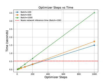
Refer to caption
(a) Optimizing time and steps
Refer to caption
(b) Sampling time and steps
Figure 5: Sampling/optimizing steps and time (in seconds). (a). The correlation between the number of optimizing steps and the corresponding optimizing time for GMS. Notably, the optimizing. (b). The correlation between the number of sampling steps and the corresponding sampling time for a single batch is observed. Notably, the sampling time demonstrates nearly linear growth with the increase in the number of sampling steps for both solvers.

Since many parts in the GMS introduce additional computational effort, Fig. 6 provides detailed information on the additional computational time of the GMS and SN-DDPM relative to the DDPM, assuming that the inference time of the noise network is unit one.

Emphasizing that the extra time is primarily for reference, most pixels can work well with a Gaussian distribution. By applying a threshold and optimizing only when the disparity between the reverse transition kernel and Gaussian exceeds it, we can conserve about 4%percent\% of computational resources without compromising result quality.

Refer to caption
Figure 6: Time cost distribution for GMS.

E.7 The reduction in the FID on CIFAR10 for GMS compared to SN-DDPM

To provide a more intuitive representation of the improvement of GMS compared to SN-DDPM at different sampling steps, we have constructed Fig. 7 below. As observed from Fig. 7, GMS exhibits a more pronounced improvement when the number of sampling steps is limited. However, as the number of sampling steps increases, the improvement of GMS diminishes, aligning with the hypothesis of our non-Gaussian reverse transition kernel as stated in the main text. However, we respectively clarify that due to the nonlinear nature of the FID metric, the relative/absolute FID improvements are not directly comparable across different numbers of steps

Refer to caption
Figure 7: The reduction in the FID on CIFAR10 for GMS compared to SN-DDPM. With a restricted number of sampling steps, the improvement exhibited by GMS surpasses that achieved with an ample number of sampling steps.

E.8 Additional results with latent diffusion

we conduct an experiment on ImageNet 256 ×\times 256 with the backbone noise network as U-ViT-Huge [4]. We train extra the second-order and the third-order noise prediction heads with two transformer blocks with the frozen backbone. The training iterations for each head is 150K and other training parameters are the same as the training of the backbone of U-ViT-Huge (details in [4]). We will evaluate the sampling efficiency of GMS under conditional sampling (classifier-free guidance scale is 0.4) and unconditional sampling in Tab. 9

Table 9: Comparison with DDPM and SN-DDPM w.r.t. FID score \downarrow on ImageNet 256 ×\times 256 by using latent diffusion. Uncond denotes the unconditional sampling, and Cond denotes sampling combining 90%percent\% conditional sampling with classifier-free guidance equals 0.4 and 10%percent\% unconditional sampling, consistent with Bao et al. [4].

Cond, CFG=0.4 Uncond
# timesteps K𝐾K 15 20 25 40 50 100 200 25 40 50 100
DDPM, β~tsubscript~𝛽𝑡\tilde{\beta}_{t} 6.48 5.30 4.86 4.42 4.27 3.93 3.32 8.62 6.47 5.97 5.04
SN-DDPM 4.40 3.36 3.10 2.99 2.97 2.93 2.82 8.19 5.73 5.32 4.60
GMS (ours) 4.01 3.07 2.89 2.88 2.85 2.81 2.74 7.78 5.42 5.03 4.45

E.9 Additional results with same calculation cost

Since GMS will cost more computation in the process of fitting the Gaussian mixture, we use the maximum amount of computation required (i.e., an additional 10% of computation is needed) for comparison, and for a fair comparison, we let the other solvers take 10% more sampling steps. Our GMS still outperforms existing SDE-based solvers with the same (maximum) computation cost in Tab. 10.

Table 10: Fair comparison with competitive SDE-based solvers w.r.t. FID score \downarrow on CIFAR10. SN-DDPM denotes Extended AnalyticDPM from [2]. The number of sampling steps for the GMS is indicated within parentheses, while for other solvers, it is represented outside of parentheses.

CIFAR10 (LS)
# timesteps K𝐾K 11(10) 22(20) 28(25) 44(40) 55(50) 110(100) 220(200) 1000(1000)
SN-DDPM 17.56 7.74 6.76 4.81 4.23 3.60 3.20 3.65
GMS (ours) 17.43 7.18 5.96 4.52 4.16 3.26 3.01 2.76

In order to provide a more intuitive representation for comparing different methods under the same sampling time, we have generated Fig. 8. Subfig. (a) of Fig. 8 illustrates that at each step, there is an additional computational time cost incurred for GMS to fit the Gaussian mixture transition kernel. This computational overhead exhibits a nearly linear growth pattern with the increase in the number of sampling steps.

Subfig. (b) of Fig. 8 offers a valuable perspective on the connection between approximate sampling time and sampling quality for two GMS and SN-DDPM. It becomes apparent that GMS consistently exhibits superior performance when compared to SN-DDPM with identical computational resources. Furthermore, the data reveals that the magnitude of improvement introduced by GMS is more substantial when the number of sampling steps is limited, as opposed to scenarios with a higher number of sampling steps.
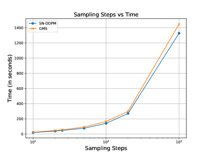
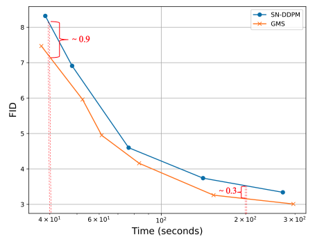
Refer to caption
(a) Sampling steps and sampling time
Refer to caption
(b) sampling time and quality
Figure 8: (a). The correlation between the number of sampling steps and the corresponding sampling time for a single batch is observed. Notably, the sampling time demonstrates nearly linear growth with the increase in the number of sampling steps for both solvers.(b).The relation between the sample quality (in FID) and the sampling time (in seconds) of GMS and SN-DDPM on CIFAR10.)

E.10 Compare with continuous time SDE-based solvers

For completeness, we compare the sampling speed of GMS and non-improved reverse transition kernel in Tab. 11, and it can be seen that within 100 steps, our method outperforms other SDE-based solvers. It is worth noting that the EDM-SDE [18] is based on the x0subscript𝑥0x_{0} prediction network, while SEED [10] and GMS are based on Ho et al. [14]’s pre-trained model which is a discrete-time noise network.

Table 11: Comparison with SDE-based solvers [18, 10] w.r.t. FID score \downarrow on CIFAR10.

CIFAR10
# timesteps K𝐾K 10 20 40 50 100
SEED-2 [10] 481.09 305.88 51.41 11.10 3.19
SEED-3 [10] 483.04 462.61 247.44 62.62 3.53
EDM-SDE [18] 35.07 14.04 9.56 5.12 2.99
GMS (ours) 17.43 7.18 4.52 4.16 3.26

E.11 Codes and License

In Tab.12, we list the code we used and the license.

Table 12: codes and license.

URL Citation License
https://github.com/w86763777/pytorch-ddpm Ho et al. [14] WTFPL
https://github.com/openai/improved-diffusion Nichol and Dhariwal [30] MIT

Appendix F SDEdit

Fig. 9 illustrates one of the comprehensive procedures of SDEdit. Given a guided image, SDEdit initially introduces noise at the level of σt0subscript𝜎subscript𝑡0\sigma_{t_{0}} to the original image x0subscript𝑥0x_{0}, where σ𝜎\sigma denotes the noise schedules of forward process in diffusion models. Subsequently, using this noisy image xt0subscript𝑥subscript𝑡0x_{t_{0}} and then discretizes it via the reverse SDE to generate the final image. Fig. 9 shows that the choice of t0subscript𝑡0t_{0} will can greatly will greatly affect the realism of sample images. With the increase of t0subscript𝑡0t_{0}, the similarity between sample images and the real image is decreasing. Hence, apart from conducting quantitative evaluations to assess the fidelity of the generated images, it is also crucial to undertake qualitative evaluations to examine the outcomes associated with different levels of fidelity. Taking all factors into comprehensive consideration, we have selected the range of t0subscript𝑡0t_{0} from 0.3T to 0.5T in our experiments.

Refer to caption
Figure 9: t0subscript𝑡0t_{0} denotes the timestep to noise the stroke

Besides experiments on LSUN 256×\times256, we also carried out an experiment of SDEdit on ImageNet 64×\times64. In Tab. 13, we show the FID score for different methods in different t0subscript𝑡0t_{0} and different sample steps. Our method outperforms other SDE-based solvers as well.

Table 13: Comparison with competitive methods in SDEdit w.r.t. FID score \downarrow on ImageNet 64×\times64. ODE-based solver is worse than all SDE-based solvers. With nearly the same computation cost, our GMS outperforms existing methods in most cases.

ImageNet 64X64, t0=1200subscript𝑡01200t_{0}=1200
# K𝐾K 26(28) 51(55) 101(111) 201(221)
DDPM,β~nsubscript~𝛽𝑛\tilde{\beta}_{n} 21.37 19.15 18.85 18.15
DDIM 21.87 21.81 21.95 21.90
SN-DDPM 20.76 18.67 17.50 16.88
GMS 20.50 18.37 17.18 16.83

Appendix G Samples

From Fig. 10 to Fig. 12, we show generated samples of GMS under a different number of steps in CIFAR10 and ImageNet 64×\times64. Here we use K𝐾K to denote the number of steps for sampling.
Refer to caption
(a) GMS (K=10𝐾10K=10)
Refer to caption
(b) GMS (K=20𝐾20K=20)
Refer to caption
(c) GMS (K=25𝐾25K=25)
Refer to caption
(d) GMS (K=40𝐾40K=40)
Refer to caption
(e) GMS (K=50𝐾50K=50)
Refer to caption
(f) GMS (K=100𝐾100K=100)
Refer to caption
(g) GMS (K=200𝐾200K=200)
Refer to caption
(h) GMS (K=1000𝐾1000K=1000)
Figure 10: Generated samples on CIFAR10 (LS)
Refer to caption
(a) GMS (K=25𝐾25K=25)
Refer to caption
(b) GMS (K=50𝐾50K=50)
Refer to caption
(c) GMS (K=100𝐾100K=100)
Figure 11: Generated samples on ImageNet 64×\times64.
Refer to caption
(a) GMS (K=200𝐾200K=200)
Refer to caption
(b) GMS (K=400𝐾400K=400)
Refer to caption
(c) GMS (K=4000𝐾4000K=4000)
Figure 12: Generated samples on ImageNet 64×\times64.