Onsager–Machlup functional for $\text{SLE}_{\kappa}$ loop measures

Abstract.

We relate two ways to renormalize the Brownian loop measure on the Riemann sphere. One by considering Brownian loop measure on the sphere minus a small disk which is known as the normalized Brownian loop measure; the other one by taking the measure on simple loops induced by the outer boundary of the Brownian loops, known as Werner’s measure. This result allows us to interpret the Loewner energy as an Onsager–Machlup functional for SLE_κ loop measure for any fixed $\kappa\in(0,4]$, and more generally, for any Malliavin–Kontsevich–Suhov loop measure of the same central charge.

1. Introduction

Onsager–Machlup functionals were introduced in [12, 11] to determine the most probable path of a diffusion process and can be considered as a probabilistic analogue of the Lagrangian of a dynamical system. For instance, let $\{B_{t}\}_{0\leqslant t\leqslant 1}$ be a standard real-valued Brownian motion and $\phi$ be a smooth real-valued curve starting at the origin. Then

(1.1) $$\lim_{\varepsilon\rightarrow 0}\frac{\mathbb{P}\left(\max_{0\leqslant t\leqslant 1}|B_{t}-\phi_{t}|<\varepsilon\right)}{\mathbb{P}\left(\max_{0\leqslant t\leqslant 1}|B_{t}|<\varepsilon\right)}=\exp\left(-\mathcal{O}(\phi)\right),$$

where $\mathcal{O}(\phi)$ is the Onsager–Machlup functional with respect to the sup-norm. For a Brownian motion $\mathcal{O}(\phi)=\frac{1}{2}\int_{0}^{1}\phi^{\prime}(t)^{2}dt$ is the Dirichlet energy of the curve $\phi$. One can consider (1.1) for different classes of stochastic processes, or smoothness of the curve $\phi$, and finally for tubes around the trajectories defined by different norms, see, [22, 10, 16, 2, 1]. A simple change of variable gives for $\kappa>0$,

(1.2) $$\lim_{\varepsilon\rightarrow 0}\frac{\mathbb{P}\left(\max_{0\leqslant t\leqslant 1}|\sqrt{\kappa}B_{t}-\phi_{t}|<\varepsilon\right)}{\mathbb{P}\left(\max_{0\leqslant t\leqslant 1}|\sqrt{\kappa}B_{t}|<\varepsilon\right)}=\exp\left(-\frac{\mathcal{O}(\phi)}{\kappa}\right).$$

Let $\nu^{\kappa}$ denote the law of $\sqrt{\kappa}B$ on the space $W_{0}([0,1],\mathbb{R})$ of real-valued continuous functions starting from zero. Then (1.2) can be restated as

(1.3) $$\lim_{\varepsilon\rightarrow 0}\frac{\nu^{\kappa}\left(D_{\varepsilon}(\phi)\right)}{\nu^{\kappa}\left(D_{\varepsilon}(0)\right)}=\exp\left(-\frac{\mathcal{O}(\phi)}{\kappa}\right),$$

where $D_{\varepsilon}(\phi)$ denotes the ball of radius $\varepsilon$ in $W_{0}([0,1],\mathbb{R})$ with respect to the sup-norm centered at $\phi\in W_{0}([0,1],\mathbb{R})$.

The goal of this work is to identify the Onsager–Machlup functional for SLE_κ loop measures. The SLE_κ loop measure is a one-parameter family (indexed by $0<\kappa\leq 4$) of infinite, $\sigma$-finite measures on simple loops in the Riemann sphere $\widehat{\mathbb{C}}=\mathbb{C}\cup\{\infty\}$, which is moreover invariant under conformal automorphisms of $\widehat{\mathbb{C}}$ (for $4<\kappa<8$ the SLE loop is non-simple). It is constructed in [23] by Zhan as a natural loop analog of the chordal SLE_κ curve connecting two boundary points of a simply connected domain by Schramm [15]. The SLE loop measure exhibits more symmetries as it does not have any distinguished marked point (as opposed to the boundary points of chordal SLE).

To state our main theorem, let us first identify the set of neighborhoods in the space of simple loops that we consider. Let $\gamma$ be an analytic loop such that $\gamma=f(S^{1})$ for some conformal map $f$ defined on $\mathbb{A}_{r}=\{z\in\mathbb{C}\,|\,r<|z|<1/r\}$ for some $0<r<1$. For $0<\varepsilon<1-r$, set $A_{\varepsilon}:=\mathbb{A}_{1-\varepsilon}$ and let us consider the neighborhoods of $S^{1}$ and $\gamma$ given by

$$O_{\varepsilon}(S^{1}):=\left\{\text{non-contractible simple loops in }A_{\varepsilon}\right\},$$

(1.4) $$O_{\varepsilon}(\gamma):=\left\{\text{non-contractible simple loops in }f(A_{\varepsilon})\right\}.$$

We call the sets of simple loops of the form $O_{\varepsilon}(\gamma)$ as admissible neighborhoods. We show that such neighborhoods are not so scarce, in fact, they form a basis of the topology induced by the Hausdorff metric on $\widehat{\mathbb{C}}$ (Proposition 2.6).

The following is our main theorem.

Theorem 1.1.

Let $\kappa\leq 4$ and $\mu^{\kappa}$ be the $\operatorname{SLE}_{\kappa}$ loop measure. For any analytic simple loop $\gamma$ and a collection of admissible neighborhoods $(O_{\varepsilon}(\gamma))_{0<\varepsilon\ll 1}$ defined as above, we have that

(1.5) $$\lim_{\varepsilon\rightarrow 0}\frac{\mu^{\kappa}\left(O_{\varepsilon}(\gamma)\right)}{\mu^{\kappa}\left(O_{\varepsilon}(S^{1})\right)}=\exp\left(\frac{c(\kappa)}{24}I^{L}(\gamma)\right),$$

where $c(\kappa):=(6-\kappa)(3\kappa-8)/2\kappa$ is the central charge of $\operatorname{SLE}_{\kappa}$ and $I^{L}(\gamma)$ is the Loewner energy of $\gamma$.

In other words, the functional $\frac{c(\kappa)}{24}I^{L}$ can then be viewed as an Onsager–Machlup-like functional for the $\text{SLE}_{\kappa}$ loop measure on the space of simple loops.

Remark.

We note that $\operatorname{SLE}_{\kappa}$ loop has the Loewner driving function $\sqrt{\kappa}B$ where $B$ is a two-sided standard Brownian motion on $\mathbb{R}$, and $I^{L}(\gamma)$ is defined as the Dirichlet energy of the driving function of $\gamma$ as introduced in [14, 18]. In light of (1.3), a natural guess for the asymptotics (1.5) would be

$$\lim_{\varepsilon\rightarrow 0}\frac{\mu^{\kappa}\left(O_{\varepsilon}(\gamma)\right)}{\mu^{\kappa}\left(O_{\varepsilon}(S^{1})\right)}=\exp\left(-\frac{I^{L}(\gamma)}{\kappa}\right).$$

Theorem 1.1 shows this guess is only true in the large deviation regime since $c(\kappa)\sim-24/\kappa$ as $\kappa\to 0{\scriptstyle+}$, see [20] for a survey on large deviation principles of SLE. For $8/3<\kappa\leq 4$, $c(\kappa)\in(0,1]$ even has a different sign than $-1/\kappa$. Theorem 1.1 is expected heuristically, given the expression of the Loewner energy in terms of determinants of Laplacians as shown in [18] and partition functions of SLE [3]. The Loewner energy also appears in various other context, see, e.g., [17, 5].

Remark.

The proof of Theorem 1.1 only uses the fact that SLE_κ loop measure is a Malliavin–Kontsevich–Suhov loop measure (introduced in [6] and proved in [23] for SLE loops) with central charge $c(\kappa)$. It is not yet known if there is a unique Malliavin–Kontsevich–Suhov loop measure for a given central charge up to scaling factor. A priori, our result applies more generally to any Malliavin–Kontsevich–Suhov loop measure.

Malliavin–Kontsevich–Suhov loop measure is characterized by a property, known as the conformal restriction covariance, stated using the normalized Brownian loop measure $\Lambda^{\ast}$ introduced in [4]. Let $V_{1}$ and $V_{2}$ be two disjoint compact non-polar subsets of $\widehat{\mathbb{C}}$, $\Lambda^{\ast}(V_{1},V_{2})\in\mathbb{R}$ is defined as a renormalization of total mass of loops intersecting both $V_{1}$ and $V_{2}$ under Brownian loop measure. See Section 2.1 for more details.

On the other hand, the Loewner energy for simple loops satisfies a similar conformal restriction property stated with the Werner’s measure $\mathcal{W}$ introduced in [21]. Werner’s measure is an infinite measure on simple loops and is obtained as the outer boundary of the Brownian loops in $\mathbb{C}$ and coincides with a multiple of the SLE_8/3 loop measure. We write $\mathcal{W}(V_{1},V_{2})$ as the total mass of loops under Werner’s measure intersecting both $V_{1}$ and $V_{2}$.

More precisely, if $\gamma$ is a simple loop with finite energy and $f:A\rightarrow f(A)$ is a conformal map on an annular neighborhood $A$ of $\gamma$, then [19, Theorem 4.1] shows

(1.6) $$I^{L}(f(\gamma))-I^{L}(\gamma)=12\mathcal{W}\left(\gamma,A^{c}\right)-12\mathcal{W}(f(\gamma),f(A)^{c}),$$

where $A^{c}:=\widehat{\mathbb{C}}\setminus A$.

A key step of the proof of Theorem 1.1 is to relate $\Lambda^{\ast}(V_{1},V_{2})$ to $\mathcal{W}(V_{1},V_{2})$ and then use the the conformal restriction property for both SLE loop measure and Loewner energy.

Theorem 1.2 (See Lemma 2.2 and Corollary 2.4).

In general, $\Lambda^{\ast}(V_{1},V_{2})$ and $\mathcal{W}(V_{1},V_{2})$ are not equal. For instance, let $K$ be a non-polar compact set and $\{K_{n}\}_{n\in\mathbb{N}}$ be a decreasing family of compact non-polar subsets shrinking to a point and disjoint from $K$. Then

$$\lim_{n\rightarrow\infty}\Lambda^{\ast}\left(K,K_{n}\right)=-\infty, \lim_{n\rightarrow\infty}\mathcal{W}\left(K,K_{n}\right)=0.$$

However, let $A$ be an annulus, $\gamma\subset A$ be a simple loop, and $f:A\rightarrow f(A)$ be a conformal map. Then we have that

(1.7) $$\mathcal{W}\left(\gamma,A^{c}\right)-\mathcal{W}(f(\gamma),f(A)^{c})=\Lambda^{\ast}\left(\gamma,A^{c}\right)-\Lambda^{\ast}(f(\gamma),f(A)^{c}).$$

See Theorem 2.3 for a more general result.

2. Brownian loop measure and Werner measure

2.1. Brownian loop measure

In this section, we recall definition and main features of the Brownian loop measure on Brownian-type non-simple loops and Werner’s measure on SLE_8/3-type simple loops.

The Brownian loop measure $\mu^{\operatorname{BL}}$ on the Riemann sphere $\widehat{\mathbb{C}}$ was introduced by Lawler and Werner in [8] using an integral of weighted two-dimensional Brownian bridges, and its definition can be easily generalized to any Riemannian surface. See, e.g., [19, Sec. 2]. For an open set $D\subset\widehat{\mathbb{C}}$, we write $\mu^{\operatorname{BL}}_{D}$ for the measure $\mu^{\operatorname{BL}}$ restricted to the loops contained in $D$. The Brownian loop measure satisfies the following properties:

-Restriction invariance: if $D^{\prime}\subset D$, then $\mathrm{d}\mu_{D^{\prime}}^{\operatorname{BL}}(\cdot)=1_{\cdot\subset D^{\prime}}\,\mathrm{d}\mu_{D}^{\operatorname{BL}}(\cdot)$.

-Conformal invariance: if $D$ and $D^{\prime}$ are conformally equivalent domains in the plane, the pushforward of $\mu_{D}^{\operatorname{BL}}$ via any conformal map from $D$ to $D^{\prime}$, is exactly $\mu_{D^{\prime}}^{\operatorname{BL}}$.

The mass of Brownian loops passing through one point is zero, therefore, we also consider $\mu^{\operatorname{BL}}$ as the Brownian loop measure on $\mathbb{C}$. The total mass of loops contained in $\mathbb{C}$ is infinite from both the contribution of big and small loops. To get rid of small loops, we consider $V_{1}$ and $V_{2}$ two compact disjoint non-polar subsets of $\mathbb{C}$, and let $\mathcal{L}\left(V_{1},V_{2}\right)$ be the family of loops in $\mathbb{C}$ that intersect both $V_{1}$ and $V_{2}$. But $\mu^{\operatorname{BL}}\left(\mathcal{L}\left(V_{1},V_{2}\right)\right)$ is still infinite due to the presence of big loops. In contrast, if $D$ is a proper open subset of $\mathbb{C}$ with non-polar boundary containing $V_{1}$ and $V_{2}$, then $\mu^{\operatorname{BL}}_{D}\left(\mathcal{L}\left(V_{1},V_{2}\right)\right)$ is finite (since big loops in $\mathbb{C}$ will eventually hit $\partial D$ and are not included in $\mu^{\operatorname{BL}}_{D}$). We write

$$\mathcal{B}(V_{1},V_{2};D):=\mu^{\operatorname{BL}}_{D}\left(\mathcal{L}\left(V_{1},V_{2}\right)\right).$$

The normalized Brownian loop measure $\Lambda^{\ast}$ introduced in [4] is defined by

(2.1) $$\Lambda^{\ast}\left(V_{1},V_{2}\right):=\lim_{r\rightarrow 0}\left(\mathcal{B}\left(V_{1},V_{2};\,\mathbb{D}_{r}(z_{0})^{c}\right)-\log\log\frac{1}{r}\right),$$

where $z_{0}\in\mathbb{C}$ and $\mathbb{D}_{r}(z_{0})^{c}=\widehat{\mathbb{C}}\setminus\mathbb{D}_{r}(z_{0})=\{z\in\widehat{\mathbb{C}}\,|\,|z-z_{0}|>r\}$. It was proved in [4] that the limit (2.1) converges to a finite number if $V_{1}$ and $V_{2}$ are disjoint non-polar compact subsets of $\widehat{\mathbb{C}}$, and the value does not depend on the choice of $z_{0}$. One can also choose $z_{0}=\infty$, then

(2.2) $$\Lambda^{\ast}\left(V_{1},V_{2}\right)=\lim_{R\rightarrow\infty}\left(\mathcal{B}\left(V_{1},V_{2};\,\mathbb{D}_{R}\right)-\log\log R\right),$$

where $\mathbb{D}_{R}:=\mathbb{D}_{R}(0)$.

We remark and as Lemma 2.2 shows, $\Lambda^{\ast}$ is not induced from a measure in the sense that $\Lambda^{\ast}(V_{1},V_{2})$ cannot be written as the total mass of loops intersecting $V_{1}$ and $V_{2}$ under some positive measure. Nonetheless, $\Lambda^{\ast}(\cdot,\cdot)$ satisfies Möbius invariance, that is,

$$\Lambda^{\ast}\left(A(V_{1}),A(V_{2})\right)=\Lambda^{\ast}\left(V_{1},V_{2}\right)$$

for any Möbius transformation $A$ of the Riemann sphere. Moreover, we have the following relation which follows directly from the definition.

Lemma 2.1.

Let $D^{\prime}\subset D$ be proper subdomains of $\mathbb{C}$ and $K\subset D^{\prime}$ is a non-polar compact set. Then

$$\Lambda^{\ast}(K,D^{\prime c})=\Lambda^{\ast}(K,D^{c})+\mathcal{B}(K,D\setminus D^{\prime};D).$$

The Brownian loop measure has been used in describing the conformal restriction covariance property of chordal SLE [7] while the ambient domain is the upper half-plane, hence renormalization is not needed. While we consider variants of SLE on the Riemann sphere, such as the case of whole-plane SLE in [4], the right normalization applied to Brownian loop measure so that similar conformal restriction formula holds is given by $\Lambda^{\ast}$.

2.2. SLE loop measures and conformal restriction covariance

In [23], Zhan constructed the SLE_κ loop measure and showed its conformal restriction covariance with central charge $c(\kappa)=(6-\kappa)(3\kappa-8)/2\kappa\leq 1$ for $\kappa\leq 4$. More precisely, this means a consistent family of measures $(\mu^{\kappa}_{D})_{D}$ on simple loops contained in a subdomain $D\subset\widehat{\mathbb{C}}$ which satisfies:

-Restriction covariance: for $D\subset\widehat{\mathbb{C}}$, then

(2.3) $$\frac{d\mu_{D}^{\kappa}}{d\mu^{\kappa}}\left(\cdot\right)=1_{\left\{\cdot\,\subset D\right\}}J_{\kappa}\left(\cdot,D^{c}\right),$$

where $\mu^{\kappa}=\mu^{\kappa}_{\widehat{\mathbb{C}}}$ and $J_{\kappa}\left(\cdot,D^{c}\right):=\exp\left(\frac{c(\kappa)}{2}\,\Lambda^{\ast}\left(\cdot,D^{c}\right)\right)$.

-Conformal invariance: if $D$ and $D^{\prime}$ are conformally equivalent domains in the plane, the pushforward of $\mu^{\kappa}_{D}$ via any conformal map from $D$ to $D^{\prime}$, is exactly $\mu^{\kappa}_{D^{\prime}}$.

This property is a rewriting of the property of having a trivial section in the determinant line bundle on space of simple loops as postulated in [6] by Kontsevich and Suhov, while inspired by the works of Malliavin, and that is why we say that SLE loop measure is a Malliavin–Kontsevich–Suhov measure. However, it is not known if there is a unique such measure (up to scaling) for a given central charge except the case of $\kappa=8/3$.

When $\kappa=8/3$, we have $c(\kappa)=0$. The restriction covariance becomes restriction invariance, namely,

$$\mathrm{d}\mu_{D^{\prime}}^{\kappa}(\cdot)=1_{\cdot\subset D^{\prime}}\,\mathrm{d}\mu_{D}^{\kappa}(\cdot)$$

using $J_{\kappa}\equiv 1$ and Lemma 2.1. This measure has been first studied by Werner [21] prior to the more general definition for other central charge in [6], often referred to as the Werner’s measure. Werner showed that there exists a unique (up to a scaling) measure on simple loops with the conformal and restriction invariance. We note that the same properties hold for the Brownian loop measure except that the Brownian loops are not simple. Indeed, Werner’s measure can be realized as the measure on the outer boundary of the Brownian loops under $\mu^{\operatorname{BL}}$ which pins down the scaling factor as well.

More precisely, if $V_{1}$ and $V_{2}$ are compact disjoint subsets of $\widehat{\mathbb{C}}$, then we write

(2.4) $$\mathcal{W}\left(V_{1},V_{2}\right):=\mathcal{B}\left(\left\{\text{loop }\delta\,|\,\partial\delta\cap V_{1}\neq\emptyset,\,\partial\delta\cap V_{2}\neq\emptyset\right\}\right)$$

which is finite as shown in [13, Lem. 4]. Here, $\partial\delta$ is the outer boundary of Brownian loop $\delta$, namely, the boundary of the connected component of $\widehat{\mathbb{C}}\setminus\delta$ containing $\infty$. Intuitively, one may view $\mathcal{W}(V_{1},V_{2})$ as another normalization of $\mu^{\operatorname{BL}}\left(\mathcal{L}(V_{1},V_{2})\right)$ since the big Brownian loops will have outer boundary near $\infty$ which does not hit $V_{1},V_{2}$.

2.3. Relations between $\Lambda^{\ast}$ and $\mathcal{W}$

The main result of this section is Theorem 2.3, where we prove a relation between the normalized Brownian loop measure $\Lambda^{\ast}$ and the corresponding quantity $\mathcal{W}$. Corollary 2.4 will then be used to describe the Onsager–Machlup functional for SLE_κ loop measures. First, we observe that although both $\Lambda^{\ast}$ and $\mathcal{W}$ normalize Brownian loop measure, they do not equal each other. We add the short proof for completeness.

Lemma 2.2.

Let $K$ be a compact non-polar set and $\{K_{n}\}_{n\in\mathbb{N}}$ be a decreasing family of compact non-polar sets disjoint from $K$ such that $\cap_{n\in\mathbb{N}}K_{n}$ is a singleton $\{p\}$. We have

$$\lim_{n\rightarrow\infty}\Lambda^{\ast}\left(K,K_{n}\right)=-\infty\quad\text{and }\quad\lim_{n\rightarrow\infty}\mathcal{W}\left(K,K_{n}\right)=0.$$

Proof.

By Lemma 2.1 we have that

$$\Lambda^{\ast}\left(K,K_{n}\right)-\Lambda^{\ast}\left(K,K_{n+1}\right)=\mathcal{B}\left(K,K_{n}\setminus K_{n+1};K_{n+1}^{c}\right)<\infty,$$

and hence

$$\Lambda^{\ast}\left(K,K_{1}\right)-\Lambda^{\ast}\left(K,K_{n}\right)=\sum_{k=1}^{n-1}\mathcal{B}\left(K,K_{k}\setminus K_{k+1};K_{k+1}^{c}\right)=\mathcal{B}\left(K,K_{1}\setminus K_{n};K_{n}^{c}\right),$$

and the latter diverges to $+\infty$ as $n\rightarrow\infty$. Hence $\lim_{n\rightarrow\infty}\Lambda^{\ast}\left(K,K_{n}\right)=-\infty$.

By monotone convergence theorem,

$$\lim_{n\rightarrow\infty}\mathcal{W}\left(K_{n},K\right)=\mathcal{W}\left(\bigcap_{n\in\mathbb{N}}K_{n},K\right)=\mathcal{W}\left(\{p\},K\right)=0.$$

The last equality holds since the probability of a two-dimensional Brownian motion hitting a singleton is zero. ∎

Theorem 2.3.

Let $A$ be an annulus, and $K\subset A$ be a connected compact subset not separating the two boundaries of $A$, and $f:A\rightarrow f(A)$ be a conformal map. Then

(2.5) $$\mathcal{W}\left(K,A^{c}\right)-\mathcal{W}(f(K),f(A)^{c})=\Lambda^{\ast}\left(K,A^{c}\right)-\Lambda^{\ast}(f(K),f(A)^{c})$$

Remark.

It is easy to see that the proof of Theorem 2.3 also works when $A$ is a simply connected domain. In this case, $K$ can be chosen to be any connected compact subset.

Proof.

Let $z_{0}\in A\setminus K$ be fixed, and $\varepsilon$ be small enough such that $\mathbb{D}_{\varepsilon}(z_{0})\subset A\setminus K$. Let $I(z_{0})$ be a continuous smooth path in $A$ (we call $I(z_{0})$ a stick for short) connecting $K$ to $z_{0}$, $I^{\varepsilon}(z_{0})=I(z_{0})\setminus\mathbb{D}_{\varepsilon}(z_{0})$, and define similarly $J_{1}^{\varepsilon}(z_{0})$ and $J_{2}^{\varepsilon}(z_{0})$ be two sticks disjoint from $I^{\varepsilon}(z_{0})$, and connecting $\partial\mathbb{D}_{\varepsilon}(z_{0})$ to the inner and outer boundary of $A$ respectively. This is possible since $K$ does not disconnect the two boundary components of $A$.

We write $\mathcal{W}\left(K_{1},K_{2};D\right)$ for the total mass of Werner’s measure of loops in $D$ intersecting both $K_{1}$ and $K_{2}$. Using (2.4) one has

(2.6) $$\mathcal{W}\left(K\cup I^{\varepsilon}(z_{0}),A^{c}\cup\bigcup_{i=1}^{2}J_{i}^{\varepsilon}(z_{0});\,\mathbb{D}_{\varepsilon}(z_{0})^{c}\right)=\mathcal{B}\left(K\cup I^{\varepsilon}(z_{0}),A^{c}\cup\bigcup_{i=1}^{2}J_{i}^{\varepsilon}(z_{0});\,\mathbb{D}_{\varepsilon}(z_{0})^{c}\right),$$

since $\mathbb{D}_{\varepsilon}(z_{0})^{c}$ is a simply connected domain with non-polar boundary and the sets $K\cup I^{\varepsilon}(z_{0})$ and $A^{c}\cup\bigcup_{i=1}^{2}J_{i}^{\varepsilon}(z_{0})$ are attached to the boundary of $\mathbb{D}_{\varepsilon}(z_{0})^{c}$. We can write (2.6) as

$$\mathcal{W}\left(K\cup I^{\varepsilon}(z_{0}),A^{c};\,\mathbb{D}_{\varepsilon}(z_{0})^{c}\right)+\mathcal{W}\left(K\cup I^{\varepsilon}(z_{0}),\bigcup_{i=1}^{2}J_{i}^{\varepsilon}(z_{0});\,A\setminus\mathbb{D}_{\varepsilon}(z_{0})\right)$$

$$=\mathcal{B}\left(K\cup I^{\varepsilon}(z_{0}),A^{c};\,\mathbb{D}_{\varepsilon}(z_{0})^{c}\right)+\mathcal{B}\left(K\cup I^{\varepsilon}(z_{0}),\bigcup_{i=1}^{2}J_{i}^{\varepsilon}(z_{0});\,A\setminus\mathbb{D}_{\varepsilon}(z_{0})\right),$$

and similarly

$$\mathcal{W}\left(f(K\cup I^{\varepsilon}(z_{0})),f(A)^{c};\,f(\mathbb{D}_{\varepsilon}(z_{0}))^{c}\right)$$

$$\qquad+\mathcal{W}\left(f(K\cup I^{\varepsilon}(z_{0})),\bigcup_{i=1}^{2}f(J_{i}^{\varepsilon}(z_{0}));\,f(A\setminus\mathbb{D}_{\varepsilon}(z_{0}))\right)$$

$$=\mathcal{B}\left(f(K\cup I^{\varepsilon}(z_{0})),f(A)^{c};\,f(\mathbb{D}_{\varepsilon}(z_{0}))^{c}\right)$$

$$\qquad+\mathcal{B}\left(f(K\cup I^{\varepsilon}(z_{0})),\bigcup_{i=1}^{2}f(J_{i}^{\varepsilon}(z_{0}));\,f(A\setminus\mathbb{D}_{\varepsilon}(z_{0}))\right).$$

By conformal invariance of both Werner measure and the Brownian loop measure one has

$$\mathcal{W}\left(K\cup I^{\varepsilon}(z_{0}),\bigcup_{i=1}^{2}J_{i}^{\varepsilon}(z_{0});\,A\backslash\mathbb{D}_{\varepsilon}(z_{0})\right) =\mathcal{W}\left(f(K\cup I^{\varepsilon}(z_{0})),\bigcup_{i=1}^{2}f(J_{i}^{\varepsilon}(z_{0}));\,f(A\backslash\mathbb{D}_{\varepsilon}(z_{0}))\right),$$

$$\mathcal{B}\left(K\cup I^{\varepsilon}(z_{0}),\bigcup_{i=1}^{2}J_{i}^{\varepsilon}(z_{0});\,A\backslash\mathbb{D}_{\varepsilon}(z_{0})\right) =\mathcal{B}\left(f(K\cup I^{\varepsilon}(z_{0})),\bigcup_{i=1}^{2}f(J_{i}^{\varepsilon}(z_{0}));\,f(A\backslash\mathbb{D}_{\varepsilon}(z_{0}))\right),$$

and hence by (2.6) it follows that

(2.7) $$\mathcal{W}\left(K\cup I^{\varepsilon}(z_{0}),A^{c};\,\mathbb{D}_{\varepsilon}(z_{0})^{c}\right)-\mathcal{W}\left(f(K\cup I^{\varepsilon}(z_{0})),f(A)^{c};\,f(\mathbb{D}_{\varepsilon}(z_{0}))^{c}\right)$$

$$=\mathcal{B}\left(K\cup I^{\varepsilon}(z_{0}),A^{c};\,\mathbb{D}_{\varepsilon}(z_{0})^{c}\right)-\mathcal{B}\left(f(K\cup I^{\varepsilon}(z_{0})),f(A)^{c};\,f(\mathbb{D}_{\varepsilon}(z_{0}))^{c}\right).$$

Now we will get rid of the sticks $I(z_{0})$. We decompose

$$\mathcal{W}\left(K\cup I^{\varepsilon}(z_{0}),A^{c};\,\mathbb{D}_{\varepsilon}(z_{0})^{c}\right)=\mathcal{W}\left(K,A^{c};\,\mathbb{D}_{\varepsilon}(z_{0})^{c}\right)+\mathcal{W}\left(I^{\varepsilon}(z_{0}),A^{c};\,(\mathbb{D}_{\varepsilon}(z_{0})\cup K)^{c}\right),$$

and (2.7) becomes

(2.8) $$\mathcal{W}\left(K,A^{c};\,\mathbb{D}_{\varepsilon}(z_{0})^{c}\right)-\mathcal{W}\left(f(K),f(A)^{c};\,f(\mathbb{D}_{\varepsilon}(z_{0}))^{c}\right)$$

$$\qquad+\mathcal{W}\left(I^{\varepsilon}(z_{0}),A^{c};\,(\mathbb{D}_{\varepsilon}(z_{0})\cup K)^{c}\right)-\mathcal{W}\left(f(I^{\varepsilon}(z_{0})),f(A)^{c};\,f(\mathbb{D}_{\varepsilon}(z_{0})\cup K)^{c}\right)$$

$$= \mathcal{B}\left(K,A^{c};\,\mathbb{D}_{\varepsilon}(z_{0})^{c}\right)-\mathcal{B}\left(f(K),f(A)^{c};\,f(\mathbb{D}_{\varepsilon}(z_{0}))^{c}\right)$$

$$\qquad+\mathcal{B}\left(I^{\varepsilon}(z_{0}),A^{c};\,(\mathbb{D}_{\varepsilon}(z_{0})\cup K)^{c}\right)-\mathcal{B}\left(f(I^{\varepsilon}(z_{0})),f(A)^{c};\,f(\mathbb{D}_{\varepsilon}(z_{0})\cup K)^{c}\right).$$

By monotone convergence it follows that

(2.9) $$\lim_{\varepsilon\rightarrow 0}\mathcal{W}\left(I^{\varepsilon}(z_{0}),A^{c};\,(\mathbb{D}_{\varepsilon}(z_{0})\cup K)^{c}\right)=\mathcal{W}\left(I(z_{0}),A^{c};\,(K\cup\{z_{0}\})^{c}\right)=\mathcal{W}\left(I(z_{0}),A^{c};\,K^{c}\right),$$

(2.10) $$\lim_{\varepsilon\rightarrow 0}\mathcal{B}\left(I^{\varepsilon}(z_{0}),A^{c};\,(\mathbb{D}_{\varepsilon}(z_{0})\cup K)^{c}\right)=\mathcal{B}\left(I(z_{0}),A^{c};\,K^{c}\right).$$

Taking the limit as $\varepsilon\rightarrow 0$, by (2.9) the left-hand-side of (2.8) becomes

(2.11) $$\mathcal{W}\left(K,A^{c}\right)-\mathcal{W}\left(f(K),f(A)^{c}\right)+\mathcal{W}\left(I(z_{0}),A^{c};\,K^{c}\right)-\mathcal{W}\left(f(I(z_{0})),f(A)^{c};\,f(K)^{c}\right).$$

The right-hand side of (2.8) will give terms in $\Lambda^{\ast}$. Note that $f(\mathbb{D}_{\varepsilon}(z_{0}))$ is comparable to $\mathbb{D}_{a\varepsilon}(f(z_{0}))$ for $a=|f^{\prime}(z_{0})|>0$ and $\varepsilon$ small enough since $f$ is a conformal map. We can then write the right-hand-side of (2.8) as

$$\mathcal{B}\left(K,A^{c};\,\mathbb{D}_{\varepsilon}(z_{0})^{c}\right)-\log\log\frac{1}{\varepsilon}+\log\log\frac{1}{a\varepsilon}-\mathcal{B}\left(f(K),f(A)^{c};\,f(\mathbb{D}_{\varepsilon}(z_{0}))^{c}\right)$$

$$+\mathcal{B}\left(I^{\varepsilon}(z_{0}),A^{c};\,(\mathbb{D}_{\varepsilon}(z_{0})\cup K)^{c}\right)-\mathcal{B}\left(f(I^{\varepsilon}(z_{0})),f(A)^{c};\,(f(\mathbb{D}_{\varepsilon}(z_{0}))\cup f(K))^{c}\right)$$

$$+\log\frac{\log\varepsilon}{\log a+\log\varepsilon},$$

and if we take the limit as $\varepsilon\rightarrow 0$ we get

(2.12) $$\Lambda^{\ast}\left(K,A^{c}\right)-\Lambda^{\ast}(K,f(A)^{c})+\mathcal{B}\left(I(z_{0}),A^{c};\,K^{c}\right)-\mathcal{B}\left(f(I(z_{0})),f(A)^{c};\,f(K)^{c}\right),$$

by the definition of $\Lambda^{\ast}$ and (2.10).

Finally, let $(z_{n})$ be a sequence going to $K$ along $I(z_{0})$. The above results replacing $I(z_{0})$ by $I(z_{n})$ being the path from $z_{n}$ to $K$ along $I(z_{0})$ still hold. By monotone convergence we have that

$$\mathcal{W}\left(I(z_{n}),A^{c};\,K^{c}\right)\xrightarrow[]{n\to\infty}0.$$

Similarly for $\mathcal{W}\left(f(I(z_{n})),f(A)^{c};\,f(K)^{c}\right)$, $\mathcal{B}\left(I(z_{n}),A^{c};\,K^{c}\right)$ and $\mathcal{B}\left(f(I(z_{n})),f(A)^{c};\,f(K)^{c}\right)$. We obtain that

$$\mathcal{W}\left(K,A^{c}\right)-\mathcal{W}\left(f(K),f(A)^{c}\right)=\Lambda^{\ast}\left(K,A^{c}\right)-\Lambda^{\ast}(K,f(A)^{c})$$

from the equality between (2.11) and (2.12) which concludes the proof. ∎

Corollary 2.4.

Let $\gamma$ be a non-contractible simple loop separating the two boundaries of an annulus $A$. Then

(2.13) $$\Lambda^{\ast}(\gamma,A^{c})-\Lambda^{\ast}(f(\gamma),f(A)^{c})=\mathcal{W}(\gamma,A^{c})-\mathcal{W}(f(\gamma),f(A)^{c}).$$

for any conformal map $f:A\rightarrow f(A)$.

Proof.

We parametrize $\gamma$ continuously by $[0,1]$ such that $\gamma(0)=\gamma(1)$. Let $K_{n}:=\gamma([0,1-1/n])$ and $R_{n}:=\gamma([1-1/n,1])$. Then $K_{n}$ is a compact connected set not separating the two boundaries of $A$. Hence by (2.5) one has that, for any $n\in\mathbb{N}$,

$$\mathcal{W}\left(K_{n},A^{c}\right)-\mathcal{W}(f(K_{n}),f(A)^{c})=\Lambda^{\ast}\left(K_{n},A^{c}\right)-\Lambda^{\ast}(f(K_{n}),f(A)^{c}).$$

From monotone convergence we have

$$\lim_{n\rightarrow\infty}\mathcal{W}\left(K_{n},A^{c}\right)=\mathcal{W}\left(\gamma,A^{c}\right)\quad\text{and }\quad\lim_{n\rightarrow\infty}\mathcal{W}(f(K_{n}),f(A)^{c})=\mathcal{W}\left(f(\gamma),f(A)^{c}\right).$$

For the normalized Brownian loop measure, Lemma 2.1 shows

$$\Lambda^{\ast}\left(\gamma,A^{c}\right)-\Lambda^{\ast}\left(K_{n},A^{c}\right)=\mathcal{B}\left(R_{n},A^{c};\,\widehat{\mathbb{C}}\setminus K_{n}\right).$$

Monotone convergence and the restriction invariance of Brownian loop measure shows

$$\lim_{n\rightarrow\infty}\left(\Lambda^{\ast}\left(\gamma,A^{c}\right)-\Lambda^{\ast}\left(K_{n},A^{c}\right)\right)=\mathcal{B}\left(\{\gamma(1)\},A^{c};\,\widehat{\mathbb{C}}\setminus\gamma\right)=0.$$

Similarly, $\lim_{n\rightarrow\infty}\Lambda^{\ast}(f(K_{n}),f(A)^{c})=\Lambda^{\ast}(f(\gamma),f(A)^{c})$. This completes the proof. ∎

2.4. A basis of Hausdorff topology on the space of simple loops

In this section we prove that the set of admissible neighborhoods (1.4) is a basis for the Hausdorff topology.

Definition 2.5.

The Hausdorff distance $d_{h}$ of two compact sets $K_{1},K_{2}\subset\widehat{\mathbb{C}}$ is defined as

$$d_{h}\left(K_{1},K_{2}\right):=\inf_{\varepsilon\geqslant 0}\left\{K_{1}\subset\bigcup_{x\in K_{2}}\overline{B}_{\varepsilon}(x)\text{ and }K_{2}\subset\bigcup_{x\in K_{1}}\overline{B}_{\varepsilon}(x)\right\},$$

where $B_{\varepsilon}(x)$ denotes the ball of radius $\varepsilon$ around $x\in\widehat{\mathbb{C}}$ with respect to the round metric.

The space $\mathcal{C}$ of non-empty compact subset of $\widehat{\mathbb{C}}$ endowed with the Hausdorff distance is a compact metric space. We then endow the space of simple loops $\mathcal{SL}\subset\mathcal{C}$ with the relative topology induced by $d_{h}$.

Proposition 2.6.

The set of admissible neighborhoods given by (1.4) is a basis for the Hausdorff topology on $\mathcal{SL}$.

Proof.

We show that any open set $O_{H}$ for the Hausdorff topology on $\mathcal{SL}$ is a union of admissible neighborhoods. Let $\gamma\in O_{H}$, $\Omega$ the bounded connected component of $\mathbb{C}\setminus\gamma$ and $\Omega^{c}$ the unbounded connected component.

For this, let us denote by $\gamma^{1+\delta}:=f_{+}(S_{1+\delta})$ and $\gamma^{1-\delta}=f_{-}(S_{1-\delta})$ two equipotentials on the two sides of $\gamma$, where $0<\delta<1/2$, $S_{r}=\{z\in\mathbb{C}\,|\,|z|=r\}$, $f_{+}$ is a conformal map $\mathbb{D}^{c}\to\Omega^{c}$ and $f_{-}$ a conformal map $\mathbb{D}\to\Omega$. We write $Y_{\delta}$ for the doubly connected domain bounded by $\gamma^{1+\delta}$ and $\gamma^{1-\delta}$. We now fix a small enough $\delta$ such that all non-contractible loops $\eta\subset Y_{\delta}$ are in $O_{H}$. By the uniformization theorem for doubly connected domains, there exists $0<r<1$ and a conformal map $f:\mathbb{A}_{r}\rightarrow Y_{\delta}$. Since $f^{-1}(\gamma)$ is compact, there exists a small $\varepsilon<1-r$ such that $A_{\varepsilon}:=\mathbb{A}_{1-\varepsilon}$ contains $f^{-1}(\gamma)$. Since $A_{\varepsilon}\subset\mathbb{A}_{r}$, the set

$$O_{\gamma}:=\left\{\text{non-contractible simple loops in }f(A_{\varepsilon})\right\}$$

is an admissible neighborhood contained in $O_{H}$ and containing $\gamma$. We obtain that $O_{H}=\bigcup_{\gamma\in O_{H}}O_{\gamma}$ and the set of admissible neighborhoods is a basis for the Hausdorff topology. ∎

3. Onsager–Machlup functional for SLE loop measures

The aim of this section is to prove Theorem 1.1. We begin with the following Lemma. Recall that $\mathcal{W}\left(K_{1},K_{2};D\right)\geq 0$ is the total mass of Werner’s measure of loops in $D$ intersecting both $K_{1}$ and $K_{2}$, and $\mathbb{D}_{r}=\{z\in\mathbb{C}\,|\,|z|<r\}$.

Lemma 3.1.

Let $K\subset\mathbb{D}$ be a compact set and $0<\varepsilon\ll 1$ such that $K\subset\mathbb{D}_{1-\varepsilon}$. Then

(3.1) $$\lim_{\varepsilon\rightarrow 0}\mathcal{W}\left(K,\mathbb{D}\setminus\mathbb{D}_{1-\varepsilon};\mathbb{D}\right)=0.$$

Proof.

Since Werner’s measure is the measure of the outer boundary of Brownian loops, we have that

$$\mathcal{W}\left(K,\mathbb{D}\setminus\mathbb{D}_{1-\varepsilon};\mathbb{D}\right)\leq\mathcal{B}\left(K,\mathbb{D}\setminus\mathbb{D}_{1-\varepsilon};\mathbb{D}\right).$$

Using the decomposition of Brownian loop measure into Brownian bubble measure $m_{D,z}$ introduced in [8], see, e.g., [4, Section 2.1.3] of Brownian bubbles in $D$ rooted at $z\in\partial D$, we have that

$$\mathcal{B}\left(K,\mathbb{D}\setminus\mathbb{D}_{1-\varepsilon};\mathbb{D}\right)=\frac{1}{\pi}\int_{0}^{2\pi}\int_{1-\varepsilon}^{1}m_{\mathbb{D}_{r},re^{\mathfrak{i}\theta}}(\{\text{bubbles intersecting }K\})\,rdrd\theta.$$

Since $m_{\mathbb{D}_{r},re^{\mathfrak{i}\theta}}(\{\text{bubbles intersecting }K\})$ is uniformly bounded for $r\in(1-\varepsilon,1]$ and $\theta\in[0,2\pi)$. The limit (3.1) follows. ∎

Fix $0<r<1$. Recall that we write $\mathbb{A}_{r}:=\{z\in\mathbb{C}\,|\,r<|z|<r^{-1}\}$ and $S_{r}:=\{|z|=r\}$.

Lemma 3.2.

Let $f$ be a conformal map $A:=\mathbb{A}_{r}\to\tilde{A}$ and $\gamma=f(S_{1})$. For $\varepsilon\ll 1-r$, let $A_{\varepsilon}:=\mathbb{A}_{1-\varepsilon}\subset\mathbb{A}_{r}$ and $\tilde{A}_{\varepsilon}=f(A_{\varepsilon})$. Then

$$\sup_{\eta\subset A_{\varepsilon}}\mathcal{W}\left(\eta,A^{c}\right),\inf_{\eta\subset A_{\varepsilon}}\mathcal{W}\left(\eta,A^{c}\right) \xrightarrow[]{\varepsilon\to 0{\scriptstyle+}}\mathcal{W}\left(S_{1},A^{c}\right)$$

$$\sup_{\tilde{\eta}\subset\tilde{A}_{\varepsilon}}\mathcal{W}(\tilde{\eta},\tilde{A}^{c}),\inf_{\tilde{\eta}\subset\tilde{A}_{\varepsilon}}\mathcal{W}(\tilde{\eta},\tilde{A}^{c}) \xrightarrow[]{\varepsilon\to 0{\scriptstyle+}}\mathcal{W}(\gamma,\tilde{A}^{c}).$$

Here and below, by $\eta\,\subset A_{\varepsilon}$ we always mean a non-contractible simple loop $\eta$ in $A_{\varepsilon}$.

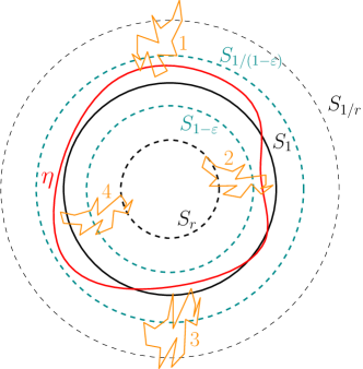
Figure 1. The Werner’s measure terms (in orange) on the right-hand-side of (3.2) numbered in order.

Proof.

To show the first limit, for $\eta\subset A_{\varepsilon}$ we write $\Omega$ for the bounded connected component of $\mathbb{C}\setminus\eta$ and $\Omega^{c}$ the unbounded component. We have

(3.2) $$|\mathcal{W}\left(\eta,A^{c}\right)-\mathcal{W}\left(S_{1},A^{c}\right)|\leq \mathcal{W}\left(\eta\cap\mathbb{D}^{c},S_{1/r};\mathbb{D}^{c}\right)+\mathcal{W}\left(\eta\cap\mathbb{D},S_{r};\mathbb{D}\right)$$

$$+\mathcal{W}\left(S_{1}\cap\Omega^{c},S_{1/r};\Omega^{c}\right)+\mathcal{W}\left(S_{1}\cap\Omega,S_{r};\Omega\right).$$

See Figure 1. We can bound these terms:

$$\mathcal{W}\left(\eta\cap\mathbb{D}^{c},S_{1/r};\mathbb{D}^{c}\right) \leq\mathcal{W}\left(S_{1/(1-\varepsilon)},S_{1/r};\mathbb{D}^{c}\right)=\mathcal{W}\left(S_{1-\varepsilon},S_{r};\mathbb{D}\right),$$

$$\mathcal{W}\left(\eta\cap\mathbb{D},S_{r};\mathbb{D}\right) \leq\mathcal{W}\left(S_{1-\varepsilon},S_{r};\mathbb{D}\right),$$

$$\mathcal{W}\left(S_{1}\cap\Omega^{c},S_{1/r};\Omega^{c}\right) \leq\mathcal{W}\left(S_{1},S_{1/r};\mathbb{D}_{1-\varepsilon}^{c}\right)\leq\mathcal{W}\left(S_{1-\varepsilon},S_{r};\mathbb{D}\right),$$

$$\mathcal{W}\left(S_{1}\cap\Omega,S_{r};\Omega\right) \leq\mathcal{W}\left(S_{1},S_{r};\mathbb{D}_{1/(1-\varepsilon)}\right)\leq\mathcal{W}\left(S_{1-\varepsilon},S_{r};\mathbb{D}\right).$$

We note that $\mathcal{W}\left(S_{1-\varepsilon},S_{r};\mathbb{D}\right)=\mathcal{W}\left(\mathbb{D}_{r},\mathbb{D}\setminus\mathbb{D}_{1-\varepsilon};\mathbb{D}\right)$. Using Lemma 3.1 and the conformal invariance of Werner’s measure, we have that the four bounds above converge to $0$ as $\varepsilon\to 0$ which concludes the proof of the first limit.

The second limit follows similarly. ∎

Now we can prove our main theorem.

Proof of Theorem 1.1.

Recall that we use the notations $A:=\mathbb{A}_{r}$, $\tilde{A}=f(\mathbb{A}_{r})$, $A_{\varepsilon}=\mathbb{A}_{1-\varepsilon}$, and $\tilde{A}_{\varepsilon}:=f(A_{\varepsilon})$, $\gamma=f(S_{1})$ and

$$O_{\varepsilon}(\gamma):=\left\{\text{non-contractible simple loops in }\tilde{A}_{\varepsilon}\right\}.$$

We write $J=J_{\kappa}$. By conformal restriction (2.3) and conformal invariance we have

$$\mu^{\kappa}(O_{\varepsilon}(\gamma))=\int 1_{\left\{\tilde{\eta}\,\subset\tilde{A}_{\varepsilon}\right\}}d\mu^{\kappa}(\tilde{\eta})=\int 1_{\left\{\tilde{\eta}\,\subset\tilde{A}_{\varepsilon}\right\}}\left(\frac{d\mu^{\kappa}_{\tilde{A}}}{d\mu^{\kappa}}(\tilde{\eta})\right)^{-1}d\mu^{\kappa}_{\tilde{A}}(\tilde{\eta})$$

$$=\int 1_{\left\{\tilde{\eta}\,\subset\tilde{A}_{\varepsilon}\right\}}J(\tilde{\eta},\tilde{A}^{c})^{-1}d\mu^{\kappa}_{\tilde{A}}(\tilde{\eta})=\int 1_{\left\{\eta\,\subset A_{\varepsilon}\right\}}J(f(\eta),\tilde{A}^{c})^{-1}d\mu^{\kappa}_{A}(\eta)$$

$$=\int 1_{\left\{\eta\,\subset A_{\varepsilon}\right\}}\frac{J(\eta,A^{c})}{J(f(\eta),\tilde{A}^{c})}d\mu(\eta).$$

By Corollary 2.4 we have that

$$\frac{J(\eta,A^{c})}{J(f(\eta),\tilde{A}^{c})} =\exp\left(\frac{c(\kappa)}{2}\,\Lambda^{\ast}\left(\eta,A^{c}\right)-\frac{c(\kappa)}{2}\,\Lambda^{\ast}(f(\eta),\tilde{A}^{c})\right)$$

(3.3) $$=\exp\left(\frac{c(\kappa)}{2}\,\mathcal{W}\left(\eta,A^{c}\right)-\frac{c(\kappa)}{2}\,\mathcal{W}(f(\eta),\tilde{A}^{c})\right).$$

It follows from Lemma 3.2 that

$$\sup_{\eta\subset A_{\varepsilon}}\left(\mathcal{W}\left(\eta,A^{c}\right)-\mathcal{W}(f(\eta),\tilde{A}^{c})\right) \xrightarrow[]{\varepsilon\to 0{\scriptstyle+}}\mathcal{W}\left(S_{1},A^{c}\right)-\mathcal{W}(\gamma,\tilde{A}^{c}),$$

$$\inf_{\eta\subset A_{\varepsilon}}\left(\mathcal{W}\left(\eta,A^{c}\right)-\mathcal{W}(f(\eta),\tilde{A}^{c})\right) \xrightarrow[]{\varepsilon\to 0{\scriptstyle+}}\mathcal{W}\left(S_{1},A^{c}\right)-\mathcal{W}(\gamma,\tilde{A}^{c}).$$

By (1.6), the limit above equals $I^{L}(\gamma)/12$ since $I^{L}(S_{1})=0$.

Hence, we have

$$\frac{\mu^{\kappa}(O_{\varepsilon}(\gamma))}{\mu^{\kappa}(O_{\varepsilon}(S_{1}))}=\frac{\int 1_{\left\{\eta\,\subset A_{\varepsilon}\right\}}\frac{J(\eta,A^{c})}{J(f(\eta),\tilde{A}^{c})}d\mu(\eta)}{\int 1_{\left\{\eta\,\subset A_{\varepsilon}\right\}}d\mu(\eta)}\xrightarrow[]{\varepsilon\to 0{\scriptstyle+}}\exp\left(\frac{c(\kappa)}{24}I^{L}(\gamma)\right)$$

which completes the proof. ∎

Acknowledgment.

We thank Fredrik Viklund and Pavel Wiegmann for helpful discussions. This work has been supported by the NSF Grant DMS-1928930 while the authors participated in a program hosted by the Simons Laufer Mathematical Sciences Institute in Berkeley, California, during the Spring 2022 semester. M.C. also acknowledges the hospitality of IHES where part of the work was accomplished during his visit there.

References

- [1] Marco Carfagnini and Maria Gordina, On the Onsager-Machlup functional for the Brownian motion on the Heisenberg group, 2023.
- [2] Ying Chao and Jinqiao Duan, The Onsager-Machlup function as Lagrangian for the most probable path of a jump-diffusion process, Nonlinearity 32 (2019), no. 10, 3715–3741. MR 4002397
- [3] Julien Dubédat, SLE and the free field: partition functions and couplings, J. Amer. Math. Soc. 22 (2009), no. 4, 995–1054. MR 2525778
- [4] Laurence S. Field and Gregory F. Lawler, Reversed radial SLE and the Brownian loop measure, J. Stat. Phys. 150 (2013), no. 6, 1030–1062. MR 3038676
- [5] Kurt Johansson, Strong Szegő theorem on a Jordan curve, Toeplitz operators and random matrices in memory of Harold Widom 289 ([2022] ©2022), 427–461. MR 4573959
- [6] Maxim Kontsevich and Yuri Suhov, On Malliavin measures, SLE, and CFT, Tr. Mat. Inst. Steklova 258 (2007), no. Anal. i Osob. Ch. 1, 107–153. MR 2400527
- [7] Gregory Lawler, Oded Schramm, and Wendelin Werner, Conformal restriction: the chordal case, J. Amer. Math. Soc. 16 (2003), no. 4, 917–955. MR 1992830
- [8] Gregory F. Lawler and Wendelin Werner, The Brownian loop soup, Probab. Theory Related Fields 128 (2004), no. 4, 565–588. MR 2045953
- [9] Yves Le Jan, Markov loops, determinants and gaussian fields, arXiv preprint math/0612112 (2006).
- [10] Terry Lyons and Ofer Zeitouni, Conditional exponential moments for iterated Wiener integrals, Ann. Probab. 27 (1999), no. 4, 1738–1749. MR 1742886
- [11] S. Machlup and L. Onsager, Fluctuations and irreversible process. II. Systems with kinetic energy, Physical Rev. (2) 91 (1953), 1512–1515. MR 0057766
- [12] by same author, Fluctuations and irreversible processes, Physical Rev. (2) 91 (1953), 1505–1512. MR 0057765
- [13] Şerban Nacu and Wendelin Werner, Random soups, carpets and fractal dimensions, J. Lond. Math. Soc. (2) 83 (2011), no. 3, 789–809. MR 2802511
- [14] Steffen Rohde and Yilin Wang, The Loewner energy of loops and regularity of driving functions, Int. Math. Res. Not. IMRN (2021), no. 10, 7715–7763. MR 4259153
- [15] Oded Schramm, Scaling limits of loop-erased random walks and uniform spanning trees, Israel J. Math. 118 (2000), 221–288. MR 1776084
- [16] L. A. Shepp and O. Zeitouni, Exponential estimates for convex norms and some applications, Barcelona Seminar on Stochastic Analysis (St. Feliu de Guíxols, 1991), Progr. Probab., vol. 32, Birkhäuser, Basel, 1993, pp. 203–215. MR 1265050
- [17] Leon A. Takhtajan and Lee-Peng Teo, Weil-Petersson metric on the universal Teichmüller space, Mem. Amer. Math. Soc. 183 (2006), no. 861, viii+119. MR 2251887
- [18] Yilin Wang, Equivalent descriptions of the Loewner energy, Invent. Math. 218 (2019), no. 2, 573–621. MR 4011706
- [19] by same author, A note on Loewner energy, conformal restriction and Werner’s measure on self-avoiding loops, Ann. Inst. Fourier (Grenoble) 71 (2021), no. 4, 1791–1805. MR 4398248
- [20] by same author, Large deviations of Schramm-Loewner evolutions: a survey, Probab. Surv. 19 (2022), 351–403. MR 4417203
- [21] Wendelin Werner, The conformally invariant measure on self-avoiding loops, J. Amer. Math. Soc. 21 (2008), no. 1, 137–169. MR 2350053
- [22] Ofer Zeitouni, On the Onsager-Machlup functional of diffusion processes around non--curves, Ann. Probab. 17 (1989), no. 3, 1037–1054. MR 1009443
- [23] Dapeng Zhan, SLE loop measures, Probab. Theory Related Fields 179 (2021), no. 1-2, 345–406. MR 4221661