Transformers as Recognizers of Formal Languages:
A Survey on Expressivity

Abstract

As transformers have gained prominence in natural language processing, some researchers have investigated theoretically what problems they can and cannot solve, by treating problems as formal languages. Exploring questions such as this will help to compare transformers with other models, and transformer variants with one another, for various tasks. Work in this subarea has made considerable progress in recent years. Here, we undertake a comprehensive survey of this work, documenting the diverse assumptions that underlie different results and providing a unified framework for harmonizing seemingly contradictory findings.

1 Introduction

Transformers (Vaswani et al., 2017) have gained prominence in natural language processing (NLP), both in direct applications like machine translation and in pretrained models like BERT (Devlin et al., 2019) and GPT (Radford et al., 2018; Brown et al., 2020; OpenAI, 2023). Consequently, some researchers have sought to investigate their theoretical properties. Such studies can broadly be divided into studies of expressivity and trainability. Studies of expressivity could be further divided into those from the perspectives of approximation theory and of formal language theory. The former (e.g., Yun et al., 2020) investigates transformers as approximators of various classes of functions, along the lines of the universal approximation theorem for feedforward neural networks (Hornik et al., 1989; Cybenko, 1989). The latter, which is the subject of this survey, investigates transformers as recognizers of formal languages – that is, the inputs are treated as sequences of discrete symbols, and crucially as sequences of unbounded length.

The core research question in this subarea is: How can we characterize the expressivity of transformers in relation to various formal models, such as automata, boolean circuits or formal logic? Related questions include:

• How do transformers compare to other architectures, like recurrent neural networks (RNNs), in expressivity?

• How do transformer variants compare to one another in expressivity?

Some further questions, which are not addressed by the papers surveyed here but could be addressed by future work in this subarea, include:

• What new transformer variants are suggested by formal models?

• Do failure cases anticipated from formal models occur in practice?

• What insights into the complexity of human language are offered by a characterization of transformer expressivity?

Interpreting theoretical transformer results is complex due to diverse assumptions. Many variants of transformers exist in practice, and even more have been proposed in theory. Also, transformers can recognize or generate languages in various ways. These diverse assumptions lead to varied, even seemingly contradictory, results.

This paper provides a comprehensive survey of theoretical results on the expressive power of transformers. Compared to the surveys of Ackerman and Cybenko (2020) and Merrill (2021, 2023), which cover convolutional neural nets (CNNs), RNNs, and transformers, this is a narrower, but deeper, survey on transformers only. It sets up a unified framework for talking about transformer variants (Section 4), reviews key topics related to formal languages (Section 6), and systematically surveys results in the literature, documenting their assumptions and claims (Section 7) and harmonizing seemingly contradictory findings. See Table 1 for a summary.

2 Overview

The work surveyed here can be classified into lower bounds (what transformers can do) and upper bounds (what transformers can’t do).

Most work on lower bounds (Section 7.2) has looked at automata like finite automata (Liu et al., 2023), counter machines (Bhattamishra et al., 2020a), and Turing machines (Pérez et al., 2021), all of which had been successfully related to RNNs before (Siegelmann and Sontag, 1995; Merrill, 2020). This wide diversity of machines is due to different transformer setups: Pérez et al. (2021) use encoder–decoders while the others use encoders only (Section 4.3).

By contrast, investigation of upper bounds has mainly focused on circuit complexity (see Section 6.2 for background), which had been successfully related to feedforward networks before (Parberry, 1994; Siu et al., 1995; Beiu and Taylor, 1996; Šíma and Orponen, 2003). This line of research, surveyed in Section 7.3, began with simplified models of transformer encoders and progressed, broadly speaking, to increasingly realistic variants and tighter bounds.

One way to restrict transformers is by discretizing the attention mechanism (Section 4.2.1). Using leftmost-hard attention, which focuses all attention on a single position, transformers cannot recognize the language Parity (Hahn, 2020) and only recognize languages in the circuit class $\mathsf{AC}^{0}$ (Hao et al., 2022). A more realistic approximation of softmax attention is average-hard attention, which can distribute attention equally across multiple positions. Average-hard attention transformers can only recognize languages in the complexity class uniform $\mathsf{TC}^{0}$ (Merrill et al., 2022; Strobl, 2023).

Alternatively, the precision of number representations can be restricted (Section 5.1). With $O(\log n)$ precision, where $n$ is the input length, softmax-attention transformers only recognize languages in uniform $\mathsf{TC}^{0}$ (Merrill and Sabharwal, 2023b, a).

More recent work has turned to formal logic as a way of characterizing the expressive power of transformers. There are many correspondences between circuit classes and logics (Section 6.4). Merrill and Sabharwal (2023a) observe that their upper bound immediately implies an upper bound of first-order logic with majority quantifiers. Alternatively, transformers can be related directly to logics; the finer control afforded by logics opens the possibility for them to be used as both upper and lower bounds (Chiang et al., 2023). Background on logic can be found in Section 6.3, and results are surveyed in Section 7.4.

3 Preliminaries

Sets

We denote by $\mathbb{N}_{0}=\{0,1,2,\ldots\}$ and $\mathbb{N}=\mathbb{N}_{0}\setminus\{0\}$ the set of natural numbers with and without $0$, respectively. We write $[n]=\{0,1,2,\ldots,n-1\}$ for any $n\in\mathbb{N}$. We write $\Sigma$ for a finite alphabet, which, in NLP applications, is the set of words or subwords known to the model.

Vectors

We use variables $d$, $d^{\prime}$, etc., for dimensionalities of vector spaces, lowercase bold letters ($\mathbf{x},\mathbf{y},\dots$) for vectors, and uppercase bold letters ($\mathbf{X},\mathbf{Y},\dots$) for matrices. For any vector $\mathbf{x}\in^{d}$, we number its elements starting from 0. For each $i\in[d]$, we write $\mathbf{x}_{i}$ or $[\mathbf{x}]_{i}$ (but not $x_{i}$) for the $i$-th component of $\mathbf{x}$.

Sequences

For any set $A$, we write ${A}^{*}$ for the set of all finite sequences over $A$. We write the length of a sequence $s\in{A}^{*}$ as $|s|$ and number its elements starting from 0; thus, $s=s_{0}s_{1}\cdots s_{|s|-1}$. We use the variable $w$ for a string in ${\Sigma}^{*}$ and $n$ for the length of $w$. For sequences in ^∗, we use lowercase bold letters ($\mathbf{x},\mathbf{y},\ldots$), and for sequences in ${{(\mathbb{R}^{d})}^{*}}$, we use the variable $X$.

A function $f\colon{A}^{*}\rightarrow{B}^{*}$ is length-preserving if $|f(w)|=|w|$ for any $w\in{A}^{*}$. For every function $g\colon A\rightarrow B$, we denote its extension to sequences by $g$ as well. That is, $g\colon{A}^{*}\rightarrow{B}^{*}$ is defined as follows: for all $s\in{A}^{*}$ and $i\in[|s|]$, $g(s)_{i}=g(s_{i})$.

Neural networks

An affine transformation is a function $L\colon\mathbb{R}^{d_{\text{in}}}\rightarrow\mathbb{R}^{d_{\text{out}}}$ parameterized by weights $\mathbf{W}_{L}\in\mathbb{R}^{{d_{\text{out}}}\times{d_{\text{in}}}}$ and bias $\mathbf{b}_{L}\in\mathbb{R}^{d_{\text{out}}}$ such that for every $\mathbf{x}\in\mathbb{R}^{d_{\text{in}}}$, $L(\mathbf{x})=\mathbf{W}_{L}\mathbf{x}+\mathbf{b}_{L}$. We say that $L$ is linear if $\mathbf{b}_{L}=\mathbf{0}$.

The activation functions we use are the rectified linear unit (ReLU) $\mathcal{R}(x)=\max(x,0)$ and the logistic sigmoid function $\mathcal{\sigma}(x)=1/(1+e^{-x})$.

The softmax function $\mathcal{S}\colon{}^{*}\rightarrow{}^{*}$ converts any sequence of reals into a probability distribution:

$$\mathcal{S}(\mathbf{x})_{i} =\frac{e^{\mathbf{x}_{i}}}{\sum_{i\in[|\mathbf{x}|]}e^{\mathbf{x}_{i}}}\qquad\forall i\in[|\mathbf{x}|].$$

4 Transformers

In this section, we give definitions for transformers and their surveyed variants, and how transformers are used to describe formal languages.

For additional background on transformers (not in relation to formal languages), Huang et al. (2022) give a lucid commentary on the original paper, Lin et al. (2022) give an overview of many variants of transformers, and Phuong and Hutter (2022) give pseudocode precisely specifying the operations of transformers. Transformers are composed of an input layer (Section 4.1), one or more hidden layers (Section 4.2), and an output layer (Section 4.3). The inputs and outputs of the layers are sequences of vectors, which we treat as members of ${{(\mathbb{R}^{d})}^{*}}$.

4.1 Input layer

Strings are initially mapped to sequences of vectors using a length-preserving function $e\colon\Sigma^{*}\rightarrow{{(\mathbb{R}^{d})}^{*}}$, which is the sum of a word embedding $\text{WE}\colon\Sigma\rightarrow\mathbb{R}^{d}$ and a position(al) embedding (or encoding) $\text{PE}_{n}\colon[n]\rightarrow\mathbb{R}^{d}$ for $n\in\mathbb{N}$:

$$e(w_{0}\cdots w_{n-1})_{i} =\text{WE}(w_{i})+\text{PE}_{n}(i).$$

In theoretical constructions, the word embedding WE can be an arbitrary computable function.

The original transformer paper (Vaswani et al., 2017) introduced the following position encoding:

$$[\text{PE}_{n}(i)]_{j}=\begin{cases}10000^{-j/d}\sin i&\text{if $j$ even}\\ 10000^{-(j-1)/d}\cos i&\text{if $j$ odd.}\end{cases}$$

Theoretical papers have explored other position encodings, including $i$ itself (Pérez et al., 2021), $i/n$ (Yao et al., 2021; Chiang and Cholak, 2022), and $1/i$ or $1/i^{2}$ (Pérez et al., 2021). Because the choice of position encoding can have a significant impact on the expressivity of the network, when stating a result, we always include the position encoding among its assumptions.

4.2 Hidden layers

A transformer layer is a length-preserving function $\mathcal{L}\colon{{(\mathbb{R}^{d})}^{*}}\rightarrow{{(\mathbb{R}^{d})}^{*}}$. There are two variants. The post-norm variant (Vaswani et al., 2017) is

$$X^{\prime} =\mathcal{N}_{1}(X+\mathcal{A}(X))$$

$$\mathcal{L}(X) =\mathcal{N}_{2}(X^{\prime}+\mathcal{F}(X^{\prime}))$$ (1)

and the pre-norm variant (Wang et al., 2019) is

$$X^{\prime} =X+\mathcal{A}(\mathcal{N}_{1}(X))$$

$$\mathcal{L}(X) =X^{\prime}+\mathcal{F}(\mathcal{N}_{2}(X^{\prime}))$$ (2)

where

• $\mathcal{A}$ is a multi-head self-attention with $d$ input/output dimensions, $H$ heads, and ${d_{\text{kv}}}$ key/value dimensions per head

• $\mathcal{F}$ is a feed-forward network (Section 4.2.2) with $d$ in/output dimensions and ${d_{\text{ff}}}$ hidden dimensions

• $\mathcal{N}_{1}$ and $\mathcal{N}_{2}$ are layernorms with $d$ dimensions.

We define each of these components below.

4.2.1 Attention

Attention was initially developed to facilitate the retrieval of previously processed data from a variable-length history (Bahdanau et al., 2015).

Transformers use a simple variant of attention known as scaled dot-product attention.

Scaled dot-product attention

A scaled dot-product attention with $d$ input/output dimensions and ${d_{\text{kv}}}$ key/value dimensions is a function ${\mathrm{A}}\colon\mathbb{R}^{d}\times{{(\mathbb{R}^{d})}^{*}}\rightarrow\mathbb{R}^{d}$ parameterized by linear transformations

$$W_{\mathrm{A}}^{\text{\kern 0.5ptQ}},W_{\mathrm{A}}^{\text{K}},W_{\mathrm{A}}^{\text{V}}\colon\mathbb{R}^{d} \rightarrow\mathbb{R}^{{d_{\text{kv}}}} W_{\mathrm{A}}^{\text{O}}\colon\mathbb{R}^{{d_{\text{kv}}}} \rightarrow\mathbb{R}^{d}$$

and defined for every $\mathbf{z}\in\mathbb{R}^{d}$, $X\in{{(\mathbb{R}^{d})}^{*}}$ (with $|X|=n$), and $j\in[n]$ as

$$\mathbf{s}(\mathbf{z},X)_{j} =\frac{W_{\mathrm{A}}^{\text{\kern 0.5ptQ}}(\mathbf{z})\cdot W_{\mathrm{A}}^{\text{K}}(X_{j})}{\sqrt{d_{\text{kv}}}}$$ (3)

$$\alpha(\mathbf{z},X) =\mathcal{S}(\mathbf{s}(\mathbf{z},X))$$ (4)

$${\mathrm{A}}(\mathbf{z},X) =W_{\mathrm{A}}^{\text{O}}\Bigl{(}\sum_{j\in[n]}\alpha(\mathbf{z},X)_{j}\,W_{\mathrm{A}}^{\text{V}}(X_{j})\Bigr{)}.$$

Typically, ${\mathrm{A}}$ is extended to a function ${\mathrm{A}}\colon{{(\mathbb{R}^{d})}^{*}}\times{{(\mathbb{R}^{d})}^{*}}\rightarrow{{(\mathbb{R}^{d})}^{*}}$ that is length-preserving in its first argument. In cross-attention, $\mathbf{z}$ is computed by the decoder while $X$ is computed by the encoder. In self-attention, the two arguments are identical:

$${\mathrm{SA}}\colon{{(\mathbb{R}^{d})}^{*}} \rightarrow{{(\mathbb{R}^{d})}^{*}}$$

$${\mathrm{SA}}(X) ={\mathrm{A}}(X,X).$$

In causally-masked (also known as future-masked) self attention, a term $m(i,j)$ is added to Eq. 3 to force every position to attend only to preceding positions:

$$m(i,j)=\begin{cases}0&\text{if $j\leq i$}\\ -\infty&\text{otherwise.}\end{cases}$$

Occasionally past-masking is used as well.

A multi-head attention with ${d_{\text{kv}}}$ key/value dimensions per head is the sum of $H$ attentions with ${d_{\text{kv}}}$ key/value dimensions:

$$\mathcal{A}(\mathbf{z},X)=\sum_{h\in[H]}{\mathrm{A}}_{h}(\mathbf{z},X).$$

Multi-head self attention is defined analogously. This is equivalent to the original formulation, which concatenated the outputs of the heads and passed them through a shared $W_{\mathrm{A}}^{\text{O}}$.

Hard attention

Some theoretical analyses of transformers simplify the model by replacing the softmax function with variants that focus attention only on the position(s) with the maximum value, differing from each other only in the way that ties are handled. For any $\mathbf{s}\in{\mathbb{R}}^{*}$, let $M(\mathbf{s})=\{i\in[|\mathbf{s}|]\mid\forall j\in[|\mathbf{s}|],\mathbf{s}_{j}\leq\mathbf{s}_{i}\}$ be the set of indices of the maximal elements of $\mathbf{s}$. In leftmost-argmax, the leftmost maximal element is used:

$$[\mathcal{S}_{\text{h}}(\mathbf{s})]_{i} =\mathbb{I}[i=\min M(\mathbf{s})]$$

whereas in average-argmax the maximal elements share weight equally:

$$[\mathcal{S}_{\text{a}}(\mathbf{s})]_{i} =\frac{\mathbb{I}[i\in M(\mathbf{s})]}{|M(\mathbf{s})|}.$$

By substituting $\mathcal{S}_{\text{h}}$ or $\mathcal{S}_{\text{a}}$ for $\mathcal{S}$ in Eq. 4, we get leftmost-hard and average-hard attention, respectively. Leftmost-hard attention was previously called hard attention by Hahn (2020) and unique hard attention by Hao et al. (2022). Average-hard attention was also called hard attention by Pérez et al. (2021) and saturated attention by Merrill et al. (2022), and has been argued to be a realistic approximation to how trained transformers behave in practice (Merrill et al., 2021).

4.2.2 Feed-forward networks

Although feed-forward networks can take many forms, in the context of transformers, we use the following definition. A feed-forward network (FFN) with $d$ input/output dimensions and ${d_{\text{ff}}}$ hidden dimensions is a function $\mathcal{F}\colon\mathbb{R}^{d}\rightarrow\mathbb{R}^{d}$ parameterized by two affine transformations, $L_{\mathcal{F}}^{1}\colon\mathbb{R}^{d}\to\mathbb{R}^{d_{\text{ff}}}$ and $L_{\mathcal{F}}^{2}\colon\mathbb{R}^{d_{\text{ff}}}\to\mathbb{R}^{d}$, such that

$$\mathcal{F}(\mathbf{x}) =L_{\mathcal{F}}^{2}(\mathcal{R}(L_{\mathcal{F}}^{1}(\mathbf{x})))$$

where $\mathcal{R}$ is applied component-wise.

4.2.3 Layer normalization

A $d$-dimensional layer normalization (Ba et al., 2016), or layernorm for short, is a function $\mathcal{N}\colon\mathbb{R}^{d}\rightarrow\mathbb{R}^{d}$ parameterized by vectors $\gamma_{\mathcal{N}},\beta_{\mathcal{N}}\in\mathbb{R}^{d}$ and $\varepsilon_{\mathcal{N}}\geq 0$:

$$\mathcal{N}(\mathbf{x})=\gamma_{\mathcal{N}}\circ\frac{\mathbf{x}-\bar{\mathbf{x}}}{\sqrt{\mathrm{var}(\mathbf{x})+\varepsilon_{\mathcal{N}}}+\beta_{\mathcal{N}}}$$

where $\circ$ is component-wise multiplication and

$$\bar{\mathbf{x}}=\frac{1}{d}\sum_{i\in[d]}\mathbf{x}_{i}\qquad\mathrm{var}(\mathbf{x})=\frac{1}{d}\sum_{i\in[d]}(\mathbf{x}_{i}-\bar{\mathbf{x}})^{2}.$$

The original definition of layernorm (Ba et al., 2016) had $\varepsilon_{\mathcal{N}}=0$, but, for numerical stability and to avoid division by zero, all implementations we are aware of set $\varepsilon_{\mathcal{N}}>0$. Observe that $\mathcal{N}$ is Lipschitz-continuous iff $\varepsilon_{\mathcal{N}}>0$.

4.3 Networks and output layers

We are now ready to give the definition of a complete transformer network.

4.3.1 Transformer encoders

A transformer encoder is a length-preserving function $\mathcal{T}\colon{\Sigma}^{*}\to{{(\mathbb{R}^{d})}^{*}}$ parameterized by the weights of an input layer $e$ and $0pt$ transformer layers $\mathcal{L}_{1},\ldots,\mathcal{L}_{0}pt$. A transformer encoder with post-norm layers is:

$$\mathcal{T}(w)=\mathcal{L}_{0pt}\circ\cdots\circ\mathcal{L}_{2}\circ\mathcal{L}_{1}\circ e(w)$$

where each $\mathcal{L}_{l}$ is a post-norm layer 1 and $\circ$ denotes function composition. A transformer encoder with pre-norm layers is additionally parameterized by the weights of a layernorm $\mathcal{N}$ and is defined as:

$$\mathcal{T}(w)=\mathcal{N}\circ\mathcal{L}_{0pt}\circ\cdots\circ\mathcal{L}_{2}\circ\mathcal{L}_{1}\circ e(w)$$

where each $\mathcal{L}_{l}$ is a pre-norm layer 2.

The encoder’s output is a sequence of vectors in ${{(\mathbb{R}^{d})}^{*}}$. To use it as a language recognizer, we add an output layer that converts $\mathcal{T}(w)$ to a probability

$$\hat{p}=\mathcal{\sigma}(\mathbf{w}\cdot[\mathcal{T}(w)]_{i}+b)$$

where $\mathbf{w}\in\mathbb{R}^{d}$, $b\in\mathbb{R}$, and $i$ is a distinguished position. The encoder accepts if $\hat{p}\geq\frac{1}{2}$ and rejects if $\hat{p}<\frac{1}{2}$.

Chiang and Cholak (2022) also consider a requirement that an encoder accepts/rejects strings with bounded cross-entropy. That is, we say that an encoder recognizes a language $L$ with cross-entropy at most $\eta$ iff for all strings $w\in L$, we have $-\log\hat{p}\leq\eta$, and for all strings $w\not\in L$, we have $-\log(1-\hat{p})\leq\eta$.

We are aware of two choices for the distinguished position $i$. Most papers use the last position ($i=n-1$) but some (Chiang and Cholak, 2022; Chiang et al., 2023), inspired by binary classifiers based on BERT (Devlin et al., 2019), prepend a special symbol CLS at position 0 and use $i=0$.

4.3.2 Transformer decoders

A transformer decoder generates rather than recognizes strings. The input is the prefix of previously-generated symbols, $w_{{}<t}=w_{0}\cdots w_{t-1}$, and the output is a probability distribution $\hat{p}(w_{t}\mid w_{{}<t})$ over the next symbol,

$$\hat{p}(\cdot\mid w_{{}<t})=\mathcal{S}(\mathbf{W}\,[\mathcal{T}(w_{{}<t})]_{t-1}+\mathbf{b})$$

where $\mathbf{W}\in\mathbb{R}^{|\Sigma|\times d}$ and $\mathbf{b}\in\mathbb{R}^{|\Sigma|}$. We assume $w_{0}=\texttt{BOS}$ and every string ends with EOS, where BOS and EOS are special symbols that do not occur anywhere else. To sample a string, we first sample $w_{1}$ from $\hat{p}(w_{1}\mid\texttt{BOS})$, then, for each time step $t>1$, sample $w_{t}$ from $\hat{p}(w_{t}\mid w_{{}<t})$. The process stops when $w_{t}=\texttt{EOS}$. Because each sampled output symbol becomes part of the input at the next time step, this kind of model is called autoregressive.

Two different ways have been proposed for defining whether a transformer decoder generates a (weighted) language.

First, Hahn (2020) considers a weighted language as a distribution over strings $p(w)$. For any length $t$, the KL divergence (relative entropy) of the model $\hat{p}(w)$ from the true distribution $p(w)$, for predicting $w_{t}$ conditioned on all previous words, is

$$\Delta_{t}[\hat{p}\mathbin{\|}p]=\sum_{w_{{}<t}}\sum_{w_{t}}p(w_{{}<t}w_{t})\log\frac{p(w_{t}\mid w_{{}<t})}{\hat{p}(w_{t}\mid w_{{}<t})}.$$

As Hahn’s results are negative, he does not spell out a positive criterion, but he seems to implicitly require that this divergence vanish at infinity:

$$\lim_{t\rightarrow\infty}\Delta_{t}[\hat{p}\mathbin{\|}p]=0.$$ (5)

Second, let us say that a transformer decoder $\varepsilon$-generates $L$ iff

$$L=\{w\mid\forall t\in[|w|],\hat{p}(w_{t}\mid w_{{}<t})\geq\varepsilon\}.$$

Then Yao et al. (2021), following Hewitt et al. (2020), say that a transformer decoder $T$ generates a language $L$ iff there exists an $\varepsilon>0$ such that $T$ $\varepsilon$-generates $L$. (This means that a transformer decoder may generate more than one language, depending on the $\varepsilon$ chosen.) They also show that any $\varepsilon$-generator can be converted into a recognizer.

While not specifically focusing on transformers, Lin et al. (2021) demonstrate limitations of autoregressive models for generation; for example, they show that there is a language $L\in\mathsf{P}$ that cannot be $\varepsilon$-generated in polynomial time for any $\varepsilon>0$ if $\mathsf{P}\neq\mathsf{NP}$.

4.3.3 Transformer encoder–decoders

A transformer encoder–decoder combines a transformer encoder and decoder, adding to each layer of the decoder an additional attention sublayer, known as cross attention, which attends to the output of the encoder.

In the literature surveyed here, only the construction of Pérez et al. (2021) and related constructions (Bhattamishra et al., 2020b; Wei et al., 2022) employ an encoder–decoder architecture. In these constructions, a string $w$ is fed to the encoder, and the decoder is allowed to run for an arbitrary number of steps. Then $w$ is accepted iff the decoder eventually outputs a vector belonging to a fixed set of accept vectors.

As we will see (Section 7.2.1), this setup vastly increases the model’s power. It could be likened to a language model that is allowed to “think step by step” (Kojima et al., 2022) before generating a final accept decision.

5 Scalability

In this section, we discuss two issues that come up frequently when trying to rigorously formulate the question of transformer expressivity.

5.1 Number representations

Transformers, like most neural networks, operate, in principle, on real numbers. While hard attention transformers could be defined using only rational numbers, even rational numbers can represent an arbitrary amount of information. In the area of expressivity of RNNs, the use of real or rational numbers has led to results that make RNNs appear more powerful in theory than in practice (Siegelmann and Sontag, 1995, 1994; Weiss et al., 2018). Consequently, some studies limit numeric representations to have $O(1)$ bits, as floating-point numbers do in practice (Chiang et al., 2023).

But the need to handle arbitrary lengths (Section 5.2) also makes it reasonable for precision to depend on $n$. Merrill and Sabharwal (2023a) argue that in $O(1)$ precision, an attention head cannot attend uniformly to a string of length $n$, because the attention weights ($\alpha$) would all round down to zero. So $O(\log n)$ bits of precision is a common choice (Yao et al., 2021; Merrill and Sabharwal, 2023b, a). Other choices are possible as well: Merrill and Sabharwal (2023b) use the set $\mathbb{F}$ of rational numbers whose denominator is unbounded but constrained to be a power of two.

Restricting the intermediate activations to limited precision introduces numerous decisions about when and how rounding should take place, which can potentially affect the expressivity of the model. For example, when summing $n$ numbers, one could round after each addition or only at the end of the summation. Better formalizing these decisions and their impact on expressivity is an area for future research.

5.2 Bounded and unbounded length

When examining transformers as language recognizers, accounting for unbounded string length is crucial. Fixing a maximum length makes all languages finite, collapsing many language classes into one. Thus, results concerning fixed or bounded lengths are beyond this survey’s scope.

It might be objected that considering unbounded lengths is too abstract, because in practice one can always fix a maximum length. But this maximum string length, driven by practical needs, seems to be growing steadily. GPT-4 has a version that uses 32,000 tokens of context, while Claude 2 uses 100,000 tokens. At the same time, some theoretical findings surveyed here seem to have practical consequences for modest string lengths. For example, we will see that there are reasons to think that in theory, transformers cannot recognize Parity for arbitrary string lengths; in practice, transformers fail to learn Parity for strings with lengths in $[2,50]$ (Bhattamishra et al., 2020a).

Some of the results surveyed here assume transformers where the position encodings (Section 4.1) or numerical precision (Section 5.1) can depend on the input length $n$. We consider these forms of length dependence to be milder than allowing the parameters themselves to depend on $n$ because they still allow inference on arbitrarily long sequences without changing any parameters of the transformer (that is, they are still a uniform model of computation).

6 Languages and Language Classes

Next, we present various formal models that transformers are compared to in the literature surveyed.

6.1 Automata and classes $\mathsf{L}$, $\mathsf{NL}$, $\mathsf{P}$

We assume familiarity with finite automata and Turing machines; for definitions, please see the textbook by Sipser (2013). Background on counter machines is given by Fischer et al. (1968). The standard deterministic model of a multi-tape Turing machine is used to define the language classes $\mathsf{L}$ (languages recognizable in space $O(\log n)$) and $\mathsf{P}$ (languages recognizable in polynomial time). The definition of $\mathsf{NL}$ (languages recognizable in non-deterministic space $O(\log n)$) uses a non-deterministic Turing machine. We also consider a random-access model of a deterministic Turing machine, which allows meaningful computation in time $O(\log n)$ (Mix Barrington et al., 1990). Problem reductions computable with bounded resources (e.g., in $\mathsf{L}$) are used to define problems complete or hard for various classes of languages.

It is known that

$$\mathsf{L}\subseteq\mathsf{NL}\subseteq\mathsf{P},$$

but none of these inclusions are known to be strict.

6.2 Circuits and classes $\mathsf{AC}^{0}$, $\mathsf{ACC}^{0}$, $\mathsf{TC}^{0}$, $\mathsf{NC}^{1}$

Circuits are a model of parallel computation particularly relevant to transformers. For more details, please see the textbook by Arora and Barak (2009).

Circuits operate on binary values. If we choose a fixed-length encoding of the symbols of $\Sigma$ as strings of $b=\lceil\log_{2}|\Sigma|\rceil$ bits, then a circuit can simulate input alphabet $\Sigma$ by encoding the value of the $i$-th input symbol into positions $ib$ to $ib+(b-1)$. For the rest of this section, we assume $\Sigma=\{0,1\}$.

Circuits

A circuit $C$ with input length $n$ is a directed acyclic graph with $n$ input vertices $s_{1},\ldots,s_{n}$ and zero or more gate vertices, each labeled by NOT, AND, or OR. Input vertices have fan-in (in-degree) zero, NOT gates have fan-in one, and the fan-in of AND and OR gates can be either two or unbounded. One (input or gate) vertex $t$ is designated the output of the circuit.

Given an input string $w\in\{0,1\}^{n}$, each input vertex $s_{i}$ is assigned the value $w_{i}$, and each gate vertex is assigned the value computed by applying its corresponding logical function to the values assigned to its in-neighbors. The circuit computes the boolean function $C\colon\{0,1\}^{n}\rightarrow\{0,1\}$, mapping each input string to the value assigned to $t$. The depth of $C$, denoted $0pt(C)$, is the length of the longest directed path from any $s_{i}$ to $t$. The size of $C$, denoted $|C|$, is the number of vertices in $C$.

Circuit families

A circuit family is a sequence $\mathcal{C}=\{C_{n}\}_{n\in\mathbb{N}}$ such that for each $n$, $C_{n}$ is a circuit with input length $n$. We treat $\mathcal{C}$ as a function on $\{0,1\}^{*}$ as follows: for every $w\in\{0,1\}^{*}$, $\mathcal{C}(w)=C_{|w|}(w)$. Then $\mathcal{C}$ defines the language $L(\mathcal{C})=\{w\in\{0,1\}^{*}\mid\mathcal{C}(w)=1\}$, and we say that $\mathcal{C}$ recognizes $L(\mathcal{C})$. The depth and size of $\mathcal{C}$ are the functions $n\mapsto 0pt(C_{n})$ and $n\mapsto|C_{n}|$.

Uniformity

As defined, a circuit family contains a different circuit for each length $n$, with no constraint on the relationship between the circuits. For example, let $L$ be any unary language: $L\subseteq\{1\}^{*}$. For $n\in\mathbb{N}$, if $1^{n}\not\in L$, define $C_{n}$ to be a circuit for the constant $0$ function (an OR gate with fan-in $0$), and if $1^{n}\in L$, define $C_{n}$ to be a circuit for the AND of all the inputs. Thus, every unary language, even an undecidable one, is recognized by a circuit family of size $O(n)$ and depth $O(1)$.

A uniformity restriction on a circuit family $\{C_{n}\}_{n\in\mathbb{N}}$ requires that the task of constructing a description of the circuit $C_{n}$ given input $n$ be computable within some specified resource bound as a function of $n$, potentially making it comparable with classes defined by bounds on Turing machine time or space. Two such uniformity bounds are used in the work we survey: space $O(\log n)$ and time $O(\log n)$. Because these bounds are very restrictive, a special representation of the circuit $C_{n}$ is used, namely, the ability to answer the questions as to the type of a gate (that is, what function it computes) and whether the output of one gate is an input to another gate.

We assume that the vertices of the circuit $C_{n}$ are numbered from $0$ to $|C_{n}|-1$. The direct connection language of a family of circuits $\cal{C}$ is the set of all tuples $\langle f,i,j,\texttt{1}^{n}\rangle$ such that in $C_{n}$, vertex $i$ has type $f$ and there is an edge from vertex $i$ to vertex $j$ (Mix Barrington et al., 1990). Given a computable function bounding the size of $\cal{C}$ and access to a membership oracle for the direct connection language, for any $n$ it is straightforward to write out the list of vertices, edges, and types in $C_{n}$.

Then a circuit family $\cal{C}$ is $\mathsf{L}$-uniform (resp., $\mathsf{DLOGTIME}$-uniform) if there is a Turing machine that runs in logarithmic space (resp., deterministic logarithmic time) to decide membership in the direct connection language of $\cal{C}$.

Circuit complexity classes

Circuit complexity classes classify circuit families and the languages they recognize based on uniformity, depth, size, fan-in bound, and the allowed gates. Since transformers have constant depth, circuit classes with constant depth are of particular interest; the classes that are used in the work we survey are:

• $\mathsf{AC}^{0}$ contains those languages that can be recognized by families of circuits with unbounded fan-in, constant depth, and polynomial size.

• $\mathsf{ACC}^{0}$ is defined analogously to $\mathsf{AC}^{0}$, but also allows gates that determine whether their inputs sum to $0$ modulo some constant.

• $\mathsf{TC}^{0}$ is defined analogously to $\mathsf{AC}^{0}$, but also allows MAJORITY gates, which have unbounded fan-in and output $1$ iff at least half of their inputs are $1$.

• $\mathsf{NC}^{1}$ is defined analogously to $\mathsf{AC}^{0}$, but with fan-in at most 2 and depth in $O(\log n)$.

The known relationships between these classes are:

$$\mathsf{AC}^{0}\subsetneq\mathsf{ACC}^{0}\subseteq\mathsf{TC}^{0}\subseteq\mathsf{NC}^{1}.$$

6.3 First-order logic

A formal language can also be defined as a set of finite strings that satisfy a closed formula of a logic. For more details, refer to Thomas (1997) or Straubing (1994).

For example, in the first-order logic of strings, or $\mathsf{FO}$, the formulas are the smallest set containing:

• Variables $x,y$, and so on.

• Atomic formulas $Q_{a}(x)$, $x=y$, $x<y$, where $a\in\Sigma$ is a symbol and $x,y$ are variables.

• $\phi_{1}\land\phi_{2}$, $\phi_{1}\lor\phi_{2}$, $\phi_{1}\rightarrow\phi_{2}$, $\neg\phi_{1}$, where $\phi_{1}$ and $\phi_{2}$ are formulas.

• $\forall x.\phi$, $\exists x.\phi$, where $x$ is a variable and $\phi$ is a formula.

Under the intended interpretation, variables stand for positions of a finite string $w$, and $Q_{a}(x)$ is true iff $w_{x}=a$. For example, $\forall x.\forall y.Q_{a}(x)\land Q_{b}(y)\rightarrow x<y$ defines the regular language $a^{\ast}b^{\ast}$. The language defined by a closed formula $\phi$ consists of those strings that satisfy $\phi$.

The languages definable in $\mathsf{FO}$ are exactly the star-free languages (McNaughton and Papert, 1971).

We are also interested in variants that add other quantifiers:

• $\mathsf{FOC}$ adds counting quantifiers $\exists^{=x}y.\phi$, which hold iff there are exactly $x$ values of $y$ that make $\phi$ true (Mix Barrington et al., 1990).

• $\mathsf{FOM}$ adds majority quantifiers $\mathsf{M}x.\phi$, which hold iff at least half of the values of $x$ make $\phi$ true (Mix Barrington et al., 1990).

We are also interested in various sets of predicates:

• Modular predicates $\mathsf{MOD}^{r}_{m}(x)$, which hold iff $x\equiv r\pmod{m}$ (Mix Barrington et al., 1992).

• $\mathsf{BIT}(x,y)$, which holds iff the $y$-th bit of $x$ is $1$.

• $\mathsf{ARB}$, the set of all possible predicates on one or more positions.

A logic extended with predicates is conventionally written with the predicates in square brackets; for example, we write $\mathsf{FO}[\mathsf{BIT}]$ for first-order logic with the $\mathsf{BIT}$ predicate.

6.4 Relationships

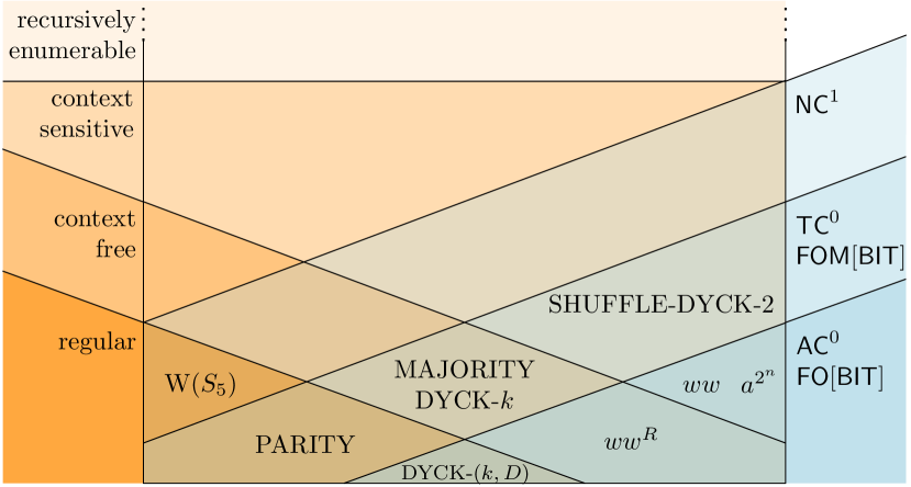
Figure 1: Relationship of some languages and language classes discussed in this paper (right) to the Chomsky hierarchy (left), assuming that $\mathsf{TC}^{0}\subsetneq\mathsf{NC}^{1}$ and $\mathsf{L}\subsetneq\mathsf{NL}$. Circuit classes are $\mathsf{DLOGTIME}$-uniform.

The relationships between the language classes defined above are depicted in Fig. 1. The classes defined by circuits/logics cut across the (perhaps more familiar) Chomsky hierarchy.

Placing some context-free languages (CFLs) outside $\mathsf{L}$-uniform $\mathsf{NC}^{1}$ depends on the widely-believed assumption that $\mathsf{L}\subsetneq\mathsf{NL}$. There exist CFLs that are hard for $\mathsf{NL}$ with respect to $\mathsf{L}$ reductions (Sudborough, 1978), so $\mathsf{CFL}\subseteq\text{$\mathsf{L}$-uniform $\mathsf{NC}^{1}$}\subseteq\mathsf{L}$ would imply $\mathsf{L}=\mathsf{NL}$.

The inclusion of $\mathsf{DLOGTIME}$-uniform $\mathsf{NC}^{1}$ in the context-sensitive languages follows from the fact that $\text{$\mathsf{DLOGTIME}$-uniform $\mathsf{NC}^{1}$}\subseteq\mathsf{L}\subseteq\mathsf{NLINSPACE}=\text{context-sensitive}$ (Kuroda, 1964).

6.4.1 Beyond $\mathsf{AC}^{0}$

The classic examples of languages not in $\mathsf{AC}^{0}$ are Parity and Majority. The language $\textsc{Parity}\subseteq\{\texttt{0},\texttt{1}\}^{*}$, contains all bit strings containing an odd number of 1’s, and $\textsc{Majority}\subseteq\{\texttt{0},\texttt{1}\}^{*}$ consists of all bit strings in which more than half of the bits are 1’s.

Other problems in $\mathsf{TC}^{0}$ but not $\mathsf{AC}^{0}$ include sorting, iterated integer addition (Chandra et al., 1984), and integer division (Hesse, 2001).

Dyck languages

The language $\textsc{Dyck-}k$ for $k>0$ is the language of strings over $k$ pairs of parentheses that are correctly balanced and nested. If we write the $i$-th parenthesis pair as $\texttt{(}_{i}\;\texttt{)}_{i}$ for each $i\in[k]$, then $\textsc{Dyck-}k$ is generated by the context-free grammar $\{S\rightarrow\texttt{(}_{i}S\texttt{)}_{i}S\mid i\in[k]\}\cup\{S\rightarrow\varepsilon\}$. These languages are of interest because any context-free language can be obtained by applying a string homomorphism to the intersection of a Dyck language with a regular language (Chomsky and Schützenberger, 1963).

Some papers surveyed here consider variations on Dyck languages. The language Dyck-$(k,D)$ for $D>0$ is the subset of Dyck-$k$ consisting of strings with maximum nesting depth $D$; it is a star-free regular language (and therefore in $\mathsf{AC}^{0}$).

The language Shuffle-Dyck-$k$ is the set of strings over $k$ pairs of parentheses in which, for each parenthesis pair, erasing the other types of parentheses leaves a correctly balanced and nested string. For example, $[(()])$ is an element of Shuffle-Dyck-2. If $k>1$, Shuffle-Dyck-$k$ is not context free.

6.4.2 Beyond $\mathsf{TC}^{0}$

As we will see (Section 7.3.2), some transformer variants lie within uniform $\mathsf{TC}^{0}$. What problems are beyond uniform $\mathsf{TC}^{0}$?

Permutations and the language $\textsc{W}(S_{5})$

A permutation of $[k]$ is a bijection $\pi\colon[k]\rightarrow[k]$, and $S_{k}$ is the set of all permutations of $[k]$. We can write one as a list, for example, $[0,3,1,2]$ is the permutation that maps $0$ to $0$, $1$ to $3$, and so on. Composition of permutations is associative but not commutative. For example (applying the permutations from left to right): $[0,2,1]\,[1,0,2]=[1,2,0]$, while $[1,0,2]\,[0,2,1]=[2,0,1]$.

By treating $S_{k}$ as an alphabet and compositions of permutations as strings, we can define the language $\textsc{W}(S_{k})$ of compositions of permutations of $[k]$ that equal the identity permutation. For example, $\textsc{W}(S_{3})$ contains $[1,0,2]\,[1,0,2]$ but not $[1,0,2]\,[0,2,1]$. This is straightforward for finite automata to recognize—each state represents the current composed permutation—but difficult when given only fixed computation depth. In particular, the language $\textsc{W}(S_{5})$ is known to be complete for $\mathsf{NC}^{1}$ under $\mathsf{DLOGTIME}$-uniform $\mathsf{AC}^{0}$ reductions (Barrington, 1989). Thus it is not in $\mathsf{DLOGTIME}$-uniform $\mathsf{TC}^{0}$ assuming that $\mathsf{TC}^{0}\subsetneq\mathsf{NC}^{1}$ (as is widely believed). This makes it a valuable example of a regular language that transformer encoders probably cannot recognize.

The languages $\textsc{W}(S_{k})$ have some relevance to natural language: Paperno (2022) study expressions like the child of the enemy of Ann where the interpretation of the child of is (roughly) a permutation of possible referents. Additionally, $\textsc{W}(S_{k})$ resembles permutation problems that have been used to benchmark transformers’ state-tracking abilities (Kim and Schuster, 2023).

Other languages

Besides $\textsc{W}(S_{5})$, other problems that are (widely believed to be) not in uniform $\mathsf{TC}^{0}$ include:

• Undirected graph connectivity, which is $\mathsf{L}$-complete (Reingold, 2008), so is not in $\mathsf{L}$-uniform $\mathsf{TC}^{0}$ unless $\mathsf{L}$-uniform $\mathsf{TC}^{0}=\mathsf{L}$.

• Solving linear equalities, which is $\mathsf{P}$-complete (Greenlaw et al., 1991), so is outside $\mathsf{L}$-uniform $\mathsf{TC}^{0}$ unless $\mathsf{L}$-uniform $\mathsf{TC}^{0}=\mathsf{P}$.

• Matrix permanent, which is known to be outside of $\mathsf{DLOGTIME}$-uniform $\mathsf{TC}^{0}$ (Allender, 1999).

6.4.3 Circuits and logics

Figure 1 indicates that $\mathsf{DLOGTIME}$-uniform $\mathsf{AC}^{0}$ and $\mathsf{TC}^{0}$ are equivalent to $\mathsf{FO}[\mathsf{BIT}]$ and $\mathsf{FOM}[\mathsf{BIT}]$, respectively. There are many such equivalences between circuit classes and logics. As a general rule of thumb, adding unbounded fan-in gates to a circuit family correlates with adding quantifiers to the corresponding logic, and increasing the degree of non-uniformity of a circuit family correlates with adding numerical predicates to the corresponding logic (Mix Barrington and Immerman, 1994). For example, making $\mathsf{AC}^{0}$ and $\mathsf{TC}^{0}$ completely non-uniform corresponds to adding arbitrary numerical predicates $(\mathsf{ARB})$ to $\mathsf{FO}$ and $\mathsf{FOM}$, respectively (Immerman, 1997; Mix Barrington et al., 1990).

As we will see below, circuits and logics each have their advantages and disadvantages for capturing the expressivity of transformers. An advantage of the circuit approach is that they have a more transparent resemblance to transformers. Transformers are computations with bounded depth, so it’s not hard to see that they should be computable by circuit families with bounded depth ($\mathsf{AC}^{0}$ or $\mathsf{TC}^{0}$). On the other hand, an advantage of the logical approach is that if we seek an exact characterization of transformers, it can be easier in a logic to add or remove quantifiers or predicates, to limit quantifier depth or number of variables, to partition terms into different sorts, and so on, than to make adjustments to a circuit family.

7 Current Results

Lower bound	Source	PE	Attention	Notes
$\ni\textsc{Majority}$	Pérez et al. 2019	none	average-hard	encoder–decoder
$\ni\textsc{Shuffle-Dyck-}k$	Bhattamishra et al. 2020a	none	softmax, masked	no residual
$\supseteq\text{SSCMs}$	Bhattamishra et al. 2020a	none	softmax, masked	no residual
$\ni\text{{Dyck}-k, depth $D$}$	Yao et al. 2021	$i/n$	leftmost-hard, masked	no layernorm, no residual
$\ni\text{{Dyck}-k, depth $D$}$	Yao et al. 2021	$i/n$	see Section 7.1.2	pre-norm
$\ni\text{{Dyck}-k}$	Yao et al. 2021	$i/n$, $i/n^{3}$, $n$	see Section 7.1.2	pre-norm
$=\mathsf{RE}$	Pérez et al. 2021	$i/n,1/i,1/{i^{2}}$	average-hard	encoder–decoder
$\supseteq\text{RASP}$	Weiss et al. 2021	$i$	average-hard	see Section 7.4.3
$\ni\textsc{Parity}$	Chiang and Cholak 2022	$i/n$	softmax	post-norm
$\supseteq\mathsf{FOC[MOD;\mathord{+}]}$	Chiang et al. 2023	sinusoidal	softmax	post-norm
Upper bound	Source	Precision	Attention	Notes
$\not\ni\textsc{Parity},\text{{Dyck}-1}$	Hahn 2020		leftmost-hard
$\not\ni\textsc{Parity},\text{{Dyck}-2}$	Hahn 2020		softmax, masked	$\varepsilon_{\mathcal{N}}>0$, vanishing KL
$\subseteq\mathsf{AC}^{0}$	Hao et al. 2022	$\mathbb{Q}$	leftmost-hard	no layernorm
$\subseteq\mathsf{TC}^{0}$	Merrill et al. 2022	$\mathbb{F}$	average-hard
$\subseteq\mathsf{FOC[MOD;\mathord{+}]}$	Chiang et al. 2023	$O(1)$	softmax
$\subseteq\text{$\mathsf{L}$-uniform~{}$\mathsf{TC}^{0}$}$	Merrill and Sabharwal 2023b	$O(\log n)$	softmax
$\subseteq\mathsf{FOM}[\mathsf{BIT}]$	Merrill and Sabharwal 2023a	$O(\log n)$	softmax
$\subseteq\text{$\mathsf{L}$-uniform~{}$\mathsf{TC}^{0}$}$	Strobl 2023	$\mathbb{F}$	average-hard

Table 1: Surveyed claims on encoder models and their assumptions. In some cases, assumptions are simplified or omitted to save space; please see main text for details.

7.1 Particular languages

7.1.1 Parity

As the classic example of a language in (uniform) $\mathsf{TC}^{0}$ but not $\mathsf{AC}^{0}$ Ajtai (1983); Furst et al. (1984), Parity is a particularly interesting case-study. Hahn (2020) showed that leftmost-hard attention transformers cannot recognize Parity, using a variant of Furst et al.’s random restriction method. He also showed that softmax attention transformers cannot generate Parity under the following two conditions:

• all position-wise functions are Lipschitz-continuous, and

• generation is defined using the KL divergence criterion in Eq. 5.

On the other hand, Chiang and Cholak (2022) showed that transformer encoders whose PE includes $i/n$ do recognize Parity. They give two constructions, corresponding to Hahn’s two assumptions. The first has Lipschitz-continuous position-wise functions, but has high cross-entropy (Section 4.3.1); as a generator, it would not meet criterion 5. The second construction uses layernorm with $\varepsilon_{\mathcal{N}}=0$, which is not Lipschitz-continuous, but it has arbitrarily low cross-entropy.

The apparent contradiction is resolved by considering the different assumptions underlying each result. The fact that Parity’s recognizability is so sensitive to assumptions suggests that it is close to the borderline of what transformer encoders can recognize. Empirically, several authors (Bhattamishra et al., 2020a; Delétang et al., 2023) have found that transformer encoders do not learn Parity.

7.1.2 Dyck languages

Hahn (2020) investigates both Dyck-1 and Dyck-2. He shows that leftmost-hard attention transformer encoders cannot recognize either one. Furthermore, he shows that softmax attention transformer encoders, under the same restrictions as for Parity (Section 7.1.1), cannot recognize Dyck-2.

Bhattamishra et al. (2020a) prove that $\textsc{Shuffle-Dyck-}k$ (which is equal to $\textsc{Dyck-}1$ when $k=1$) is recognizable by a soft-attention transformer encoder with future masking, no position encoding, no layernorm, and no residual connections.

Yao et al. (2021) study the ability of transformers to recognize Dyck languages:

• A $(D+1)$-layer encoder can recognize Dyck-$(k,D)$ using a PE including $i/n$, $O(\log n)$ precision, leftmost-hard attention with future and past masking, and neither layernorm nor residual connections.

• A $2$-layer decoder can generate Dyck-$(k,D)$ using the same PE and precision as above and layernorm and residual connections in its FFNs. It uses softmax with future masking, but also needs leftmost-hard attention, which can either be simulated (up to a maximum input length) or directly added to the model.

• A $2$-layer decoder can generate Dyck-$k$ using the same assumptions as the previous result, plus a PE including $i/n$, $i/n^{3}$, and $n$.

Ebrahimi et al. (2020) perform experiments to train transformers to recognize Dyck-$2$ and Dyck-$4$, finding that they are competitive with LSTMs, and that prepending a BOS symbol helps.

7.1.3 Other languages

The language Majority, like Parity, is not in $\mathsf{AC}^{0}$, but Pérez et al. (2019) prove that a transformer encoder (rather, a transformer encoder–decoder with a trivial decoder) without any position encoding recognizes Majority; Merrill et al. (2022) prove the same for transformer encoders.

Bhattamishra et al. (2020a) experiment with training transformer encoders on some counter languages: $\textsc{Dyck-}1$, $\textsc{Shuffle-Dyck-}k$ for $k\in\{2,4,6\}$, $k$-ary boolean expressions in prefix notation for $k\in\{3,5\}$, $\{\texttt{a}^{n}\texttt{b}^{n}$}, $\{\texttt{a}^{n}\texttt{b}^{n}\texttt{c}^{n}\}$, $\{\texttt{a}^{n}\texttt{b}^{n}\texttt{c}^{n}\texttt{d}^{n}\}$, observing nearly perfect learning and generalization to longer lengths with masking and no positional encoding. They also experiment with learning regular languages including the Tomita (1981) languages, Parity, $(\texttt{aa})^{*}$, $(\texttt{abab})^{*}$, and Dyck-$(1,D)$ for $D\in\{2,3,4,12\}$, where they find that only the star-free languages of dot-depth $1$ are learned and generalized well.

Delétang et al. (2023) study experimentally how well transformer encoders (and other networks) learn tasks at various levels of the Chomsky hierarchy, including generalization to longer strings. Languages include $\texttt{a}\Sigma^{*}\texttt{a}+\texttt{b}\Sigma^{*}\texttt{b}$, Parity and Majority. Of these three languages, they find that transformers learn only Majority.

7.2 Automata

7.2.1 Turing machines

Pérez et al. (2021) consider transformer encoder–decoders with several modifications:

• The PE includes components $i$, $1/i$, and $1/i^{2}$.

• In self attention, Eq. 3 takes the negative absolute value of the dot-product, and Eq. 4 uses average-hard attention.

• The FFNs use sigmoids instead of ReLUs.

As described above (Section 4.3.3), the decoder is allowed to run for arbitrarily many time steps until an acceptance criterion is met. Under these assumptions, transformer encoder–decoders can recognize any recursively enumerable language.

This result uses arbitrary precision, but as a corollary, Pérez et al. (2021) show that a $T(n)$-time-bounded Turing machine can be simulated in a transformer using $O(\log T(n))$ bits of precision.

Bhattamishra et al. (2020b) provide a simpler proof of Pérez et al.’s result by reducing to an RNN and appealing to the construction of Siegelmann and Sontag (1995). They do this for two sets of assumptions. First,

• The PE includes only $i$.

• The self attention sublayers are as above.

• The FFNs use saturated linear activation functions: $\sigma(x)=\max(0,\min(1,x))$.

Second,

• There is no PE.

• In self attention, Eq. 3 uses the standard dot-product and causal masking, and Eq. 4 again uses average-hard attention.

• FFNs use saturated linear activation functions.

Wei et al. (2022) define a notion of statistically-meaningful (SM) approximation and show that transformer encoder–decoders SM-approximate Turing machines. Both the decoder and Turing machine are limited to $N$ time steps; additionally,

• The position encoding can be an arbitrary computable function on $[N]$.

• Attention is average-hard.

• The FFNs have three ReLU layers.

7.2.2 Finite automata

Liu et al. (2023) study the ability of transformer decoders to simulate deterministic finite automata (DFAs), in the sense of computing not only the same acceptance decision but also the same state sequence. Although a transformer with depth $N$ can simulate a DFA for $N$ timesteps, Liu et al. show how to construct lower-depth shortcuts for subclasses roughly corresponding to classes of regular languages in Fig. 1. These constructions depend on $N$, but in the context of this survey, a noteworthy finding is that any regular language in $\mathsf{ACC}^{0}$ can be recognized up to length $N$ by a transformer decoder whose FFNs use sine activations and whose number of parameters is independent of $N$ (although the parameters themselves do depend on $N$).

7.2.3 Counter machines

Counter machines are automata with integer-valued registers, which have been studied extensively in connection with LSTM RNNs (Weiss et al., 2018; Suzgun et al., 2019; Merrill, 2019, 2020). Bhattamishra et al. (2020a), following Merrill et al. (2020), define a subclass of counter machines called simplified and stateless $k$-counter machines (SSCMs). These machines use a counter update function $u\colon\Sigma\rightarrow\mathbb{Z}^{k}$ to increment and decrement each counter based on the current input symbol, but they have no state and cannot look at the counter values until the end of the string. They then show that any SSCM can be converted to an equivalent transformer encoder with causal masking and no residual connections.

7.3 Circuits

The results in this section and the next all consider transformer encoders. For brevity, we write “transformer” to mean “transformer encoder.”

7.3.1 Boolean circuits: $\mathsf{AC}^{0}$

Hao et al. (2022) generalize the leftmost-hard attention results of Hahn (2020) to show that any language recognized by a transformer with leftmost-hard attention is in $\mathsf{AC}^{0}$. The proof gives a normal form for transformers with leftmost-hard attention and uses it to construct an $\mathsf{AC}^{0}$ circuit family. Like the leftmost-hard attention results of Hahn (2020), this result applies to a generalized model of transformers with few restrictions on the component functions. It uses the fact that only $O(\log n)$ bits of information are needed per position.

7.3.2 Threshold circuits: $\mathsf{TC}^{0}$

Merrill et al. (2022) prove an upper bound analogous to that of Hao et al. (2022), but for average-hard attention transformers. They show that a transformer with activations in $\mathbb{F}$ can be simulated in $\mathsf{TC}^{0}$. The key reason why soft attention extends the power to $\mathsf{TC}^{0}$ is because it enables counting (cf. Section 7.2.3), and counting can be used to solve problems like Majority that are outside $\mathsf{AC}^{0}$.

Furthermore, Merrill and Sabharwal (2023b) show that softmax attention, $O(\log n)$-precision transformers are in $\mathsf{L}$-uniform $\mathsf{TC}^{0}$, and Strobl (2023) shows that average-hard attention transformers are in $\mathsf{L}$-uniform $\mathsf{TC}^{0}$ as well. This uniform $\mathsf{TC}^{0}$ upper bound fits transformers into other known complexity hierarchies, revealing that transformers likely cannot solve problems complete for $\mathsf{NC}^{1}$, $\mathsf{L}$, and other classes believed to be above $\mathsf{TC}^{0}$ (Section 6.4).

7.4 Logics

7.4.1 First-order logic with majority

Merrill and Sabharwal (2023a) further tighten the $\mathsf{L}$-uniform $\mathsf{TC}^{0}$ upper bound of Merrill and Sabharwal (2023b) to $\mathsf{DLOGTIME}$-uniform $\mathsf{TC}^{0}$, and therefore $\mathsf{FOM}[\mathsf{BIT}]$. The proof constructs subroutines to answer queries about the types of nodes and connectivity of pairs of nodes in the computation graph of a transformer, and shows that these queries can be translated to queries for a $\mathsf{TC}^{0}$ circuit family with $O(\log n)$ time overhead.

7.4.2 First-order logic with counting

Chiang et al. (2023) obtain both an upper and a lower bound by defining a logic $\mathsf{FOC[MOD;\mathord{+}]}$, which is first-order logic with counting quantifiers, using two sorts for positions and counts (Immerman, 1999, p. 185–187), where positions have the $\mathsf{MOD}$ predicate (but not $<$ or $=$), and counts have $<$, $+$, and $=$, capturing the fact that transformers can add and compare activations, but not positions. They show that this logic is intermediate in expressivity between $O(1)$-precision and infinite-precision transformers. The lower-bound proof makes use of a normal form that eliminates quantifiers over counts and makes quantifiers over positions have depth 1; a perhaps surprising consequence is that $O(1)$-precision transformers are no more powerful than 2-layer uniform-attention transformers.

7.4.3 RASP

Weiss et al. (2021) define a programming language called RASP (Restricted Access Sequence Programming Language) and show that it can be compiled to transformers with average-hard attention and two extensions:

• Attention weights are directly computed from the previous layer without being confined to dot-products of query and key vectors.

• Position-wise FFNs compute arbitrary computable functions.

Lindner et al. (2023) describe a RASP compiler that outputs standard transformers. It compiles RASP selectors to dot-product attention, with syntactic restrictions on selectors and a maximum string length. Element-wise operations are approximately compiled to ReLU FFNs. Friedman et al. (2023) define Transformer Programs, a restricted class of transformers that can be translated into RASP programs.

8 Conclusions

Out of the large body of research surveyed above, we highlight several conclusions have been more or less firmly established:

1. Transformer encoder–decoders require an unbounded number of time-steps to achieve Turing-completeness. Without this, their expressivity is significantly curtailed.

2. The right frameworks for thinking about the expressivity of transformer encoders are circuits or logic, not formal grammars or automata.

3. Leftmost-hard-attention transformers are in $\mathsf{AC}^{0}$ and cannot solve some intuitively easy problems, like Parity and Majority.

4. Soft attention gives transformers the ability to count. Nevertheless, they lie within $\mathsf{TC}^{0}$ and likely cannot solve problems like $\textsc{W}(S_{5})$ and directed graph connectivity.

Some open questions that we think should be priorities for future research are:

1. Can the expressivity of softmax-attention transformers be characterized more tightly or even exactly in terms of some logic?

2. Given the current practical importance of decoder-only transformers and intense interest in chain-of-thought reasoning, what further insights can the theory of circuits or logic provide into transformer decoders?

We hope this paper can serve as a valuable resource for researchers studying transformer expressivity within formal language theory. We encourage fellow researchers to include a concise section in their future work, specifying assumptions and demonstrating alignment with the dimensions presented here in Table 1. This will aid understanding, comparing findings, and fostering insights.

References

- Ackerman and Cybenko (2020) Joshua Ackerman and George Cybenko. 2020. A survey of neural networks and formal languages. arXiv:2006.01338.
- Ajtai (1983) Miklós Ajtai. 1983. -formulae on finite structures. Ann. Pure Appl. Log., 24:1–48.
- Allender (1999) Eric Allender. 1999. The permanent requires large uniform threshold circuits. Chicago Journal of Theoretical Computer Science, 1999(7).
- Arora and Barak (2009) Sanjeev Arora and Boaz Barak. 2009. Computational Complexity: A Modern Approach. Cambridge University Press.
- Ba et al. (2016) Jimmy Lei Ba, Jamie Ryan Kiros, and Geoffrey E. Hinton. 2016. Layer normalization. In NIPS 2016 Deep Learning Symposium.
- Bahdanau et al. (2015) Dzmitry Bahdanau, Kyunghyun Cho, and Yoshua Bengio. 2015. Neural machine translation by jointly learning to align and translate. In Proceedings of the 3rd International Conference on Learning Representations (ICLR).
- Barrington (1989) David A. Barrington. 1989. Bounded-width polynomial-size branching programs recognize exactly those languages in . Journal of Computer and System Sciences, 38(1):150–164.
- Beiu and Taylor (1996) Valeriu Beiu and John G. Taylor. 1996. On the circuit complexity of sigmoid feedforward neural networks. Neural Networks, 9(7):1155–1171.