Abstract

Compression schemes have been extensively used in Federated Learning (FL) to reduce the communication cost of distributed learning. While most approaches rely on a bounded variance assumption of the noise produced by the compressor, this paper investigates the use of compression and aggregation schemes that produce a specific error distribution, e.g., Gaussian or Laplace, on the aggregated data. We present and analyze different aggregation schemes based on layered quantizers achieving exact error distribution. We provide different methods to leverage the proposed compression schemes to obtain compression-for-free in differential privacy applications. Our general compression methods can recover and improve standard FL schemes with Gaussian perturbations such as Langevin dynamics and randomized smoothing.

1 INTRODUCTION

Machine learning has become increasingly data-hungry, requiring vast amounts of data to train models effectively. Federated learning (FL) (McMahan et al., 2017; Karimireddy et al., 2020; Kairouz et al., 2021b) has emerged as a promising approach for collaborative machine learning in distributed settings. In FL, multiple parties with their local datasets participate in a joint model training process without exchanging their raw data. However, communication from these devices to a central server can be slow and expensive resulting in a bottleneck. Thus, compression schemes have been widely used to reduce the size of the updates before transmission. Standard compression schemes (Konečnỳ et al., 2016; Alistarh et al., 2017; Wen et al., 2017; Lin et al., 2018; Li et al., 2022) typically assume relatively bounded variance assumptions on the noise produced by the compressor. These schemes do not take into account the specific error distribution of the noise, which may depend on the input distribution. This can be hindering in settings where control of the noise shape can provide tighter analysis or can enable the fulfilment of additional constraints, e.g. differential privacy.

In a wider scope, different structures of the compression error have been extensively leveraged beyond FL such as in: lossy data compression for audio and music compression (Johnston, 1988; Sayood, 2017); medical imaging (Liu et al., 2017; Ammah and Owusu, 2019); error control in wireless communications (Costello et al., 1998); quantization in deep learning (Rastegari et al., 2016) with weight pruning (Han et al., 2015; Anwar et al., 2017), low-precision weights (Jacob et al., 2018; Jung et al., 2019) and data perturbation for privacy-preserving machine learning (Abadi et al., 2016). In this context, the main goal of this paper is to answer the following research questions: (i) Can we go beyond standard assumptions on the variance and ensure a particular (continuous) distribution of the compression error? (ii) What are the benefits, communication cost and applications of such schemes?

Related work. Recently, different compression techniques with a precise noise distribution have been applied to various machine learning tasks. Agustsson and Theis (2020) apply subtractively dithered quantization (Roberts, 1962; Ziv, 1985; Zamir and Feder, 1992) to ensure a uniformly distributed noise in neural compression. Relative entropy coding (Havasi et al., 2019; Flamich et al., 2020) aims at compressing the model weights and latent representations to a number of bits approximately given by their relative entropy from a reference distribution. Differential privacy can be achieved by ensuring a precise noise distribution, using lattice quantization (Amiri et al., 2021; Lang et al., 2023), minimal random coding (Shah et al., 2022), or randomized encoding (Chaudhuri et al., 2022). These methods can be regarded as examples of channel simulation (Bennett et al., 2002; Harsha et al., 2010; Li and El Gamal, 2018), which is a point-to-point compression scheme where the output follows a precise conditional distribution given the input. Refer to (Yang et al., 2023; Theis et al., 2022) for more applications of channel simulation on neural compression.

In this paper, we not only consider a point-to-point compression setting, but also a distributed mean estimation and aggregation setting (Suresh et al., 2017), which is one of the most fundamental building blocks of FL algorithms (Kairouz et al., 2021b). There are $n$ users holding the data $x_{1},\ldots,x_{n}$ respectively (which can be the gradient as in FedSGD, or the model weights as in FedAvg (McMahan et al., 2017)), who communicate with the server to allow the server to output an estimate $Y$ of the mean, with a precise noise distribution $Y-n^{-1}\sum_{i}x_{i}\sim Q$, which can then be used to perform model updates with a more precise behavior.

There are two approaches to this problem, namely individual mechanisms where point-to-point compression is performed between each user and the server, and the server simply averages the reconstructions of the data of each user (possibly with some postprocessing); and aggregate mechanisms where the encoding functions of all users are designed as a whole to ensure a precise noise distribution of the final estimate $Y$. For individual mechanisms, we study the communication costs of the direct and shifted layered quantizers based on (Wilson, 2000; Hegazy and Li, 2022). For aggregate mechanisms, we propose a novel method, called the aggregate Gaussian mechanism, to ensure that the overall noise distribution $Q$ is exactly Gaussian, and analyze its communication cost.

In particular, for differential privacy (DP), the above schemes allow us to consider two trust settings. First, for a completely trusted server, if the clients wish to prevent the output of the server from leaking information on their data $x_{1},\ldots,x_{n}$, a DP restriction (Dwork et al., 2006) can be imposed on the output $Y$. This is achieved by requiring the noise distribution $Q$ to be a privacy-preserving noise distribution. For example, a Gaussian noise can guarantee $(\varepsilon,\delta)$-DP (Dwork et al., 2014) and Rényi DP (Mironov, 2017). Second, when the server is less-trusted, the clients wish for the server to not know their individual datapoints but trust it to faithfully carry out some postprocessing to make the output DP against external observers. In this case, it is vital to ensure that the compression mechanism is homomorphic, and the messages sent from the users to the server can be aggregated before decoding, so that it is compatible with secure aggregation (SecAgg) techniques such as (Bonawitz et al., 2017) and other homomorphic cryptosystems. The aggregate Gaussian mechanism we propose is homomorphic, making it suitable for both privacy concerns of trusted and less-trusted servers.

Contributions. (1) We propose different quantized aggregation schemes based on layered quantizers that produce a specific error distribution, e.g. Gaussian or Laplace. (2) We provide theoretical guarantees and practical implementation of the developed aggregate mechanisms. (3) We exhibit FL applications in which we directly benefit from an exact Gaussian noise distribution, namely compression for free with differential privacy and compression schemes for Langevin dynamics and randomized smoothing.

Notation. The term $\log$ refers to the logarithm in base $2$ while $\ln$ denotes the natural logarithm. The floor and ceil functions are denoted by $\lfloor\cdot\rfloor$ and $\lceil\cdot\rceil$ respectively with $\lceil x\rfloor:=\lfloor x+1/2\rfloor$. For $n\in\mathbb{N}$, we refer to $\{1,\ldots,n\}$ with the notation $[n]$. For a discrete probability distribution $p_{X}$ supported on $\mathcal{X}$ and random variable $X\sim p_{X}$, $\operatorname{\mathcal{H}}(X)$ denotes the entropy of $X$, i.e. $\operatorname{\mathcal{H}}(X)=\operatorname{\mathcal{H}}(p_{X})=-\sum_{x\in\mathcal{X}}p_{X}(x)\log p_{X}(x)$. $\operatorname{\mathcal{H}}(X|Y)$ denotes the conditional entropy of $X$ given $Y$, i.e., $\operatorname{\mathcal{H}}(X|Y)=\mathbb{E}[\operatorname{\mathcal{H}}(p_{X|Y}(\cdot|Y)]$. For a continuous probability distribution $f_{X}$ supported on $\mathcal{X}$ and random variable $X\sim f_{X}$, $h(X)$ denotes the differential entropy of $X$, i.e. $h(X)=-\int_{\mathcal{X}}f_{X}(x)\log f_{X}(x)\mathrm{d}x$. The Lebesgue measure is denoted by $\lambda$ and $\mathcal{U}(a,b)$ with $a<b$ refers to the uniform distribution on $(a,b)$. All proofs, additional details and experiments are available in the appendix.

2 BACKGROUND, MOTIVATION

Quantized aggregation. Consider $n$ clients ($n\geq 1$). In the standard FL setting, the training process relies on locally generated randomness at individual participant devices. In this paper, we allow the clients and the server to have shared randomness. Practically, shared randomness can be generated by sharing a small random seed among the clients and the server, allowing them to generate a sequence of shared random numbers. We will see later that the existence of shared randomness can greatly simplify the schemes.

Let $S_{i}\in\mathcal{S}$ be the shared randomness between client $i$ and the server, and $T\in\mathcal{T}$ be the global shared randomness between all clients and the server. When building an FL algorithm, one is allowed to choose the joint distribution $P_{(S_{i})_{i},T}$ where these variables are usually (but not necessarily) taken to be mutually independent. Client $i\in[n]$ holds the data $x_{i}\in\mathbb{R}^{d}$ and for privacy and communication constraints, performs encoding to produce the description $M_{i}=\mathscr{E}(x_{i},S_{i},T)\in\mathcal{M}$, where $\mathscr{E}:\mathbb{R}^{d}\times\mathcal{S}\times\mathcal{T}\to\mathcal{M}$ is the encoding function, and $\mathcal{M}$ is the set of descriptions (usually taken to be $\mathbb{Z}^{d}$). Given the descriptions $M_{1},\ldots,M_{n}$, the server produces the reconstruction $Y=\overline{\mathscr{D}}(M_{1},\ldots,M_{n},S_{1},\ldots,S_{n},T)$ which is an estimate of the average $n^{-1}\sum_{i=1}^{n}x_{i}$, where $\overline{\mathscr{D}}:\mathcal{M}^{n}\times\mathcal{S}^{n}\times\mathcal{T}\to\mathbb{R}^{d}$ is the overall decoding function. The goal is to control the distribution of the quantization error as described in the next definition.

Definition 1.

(Aggregate AINQ mechanism) A quantization scheme with $n$ clients holding data $x_{1},\ldots,x_{n}$ and a server producing $Y$ satisfies the Additive Independent Noise Quantization (AINQ) property if the quantization error follows a target distribution $Q$ regardless of $\left\{x_{i}\right\}_{i=1}^{n}$, i.e.,

$$Y-\left(\frac{1}{n}\sum_{i=1}^{n}x_{i}\right)\sim Q.$$ (1)

A special case is when $n=1$, which we call point-to-point AINQ mechanism. In this case, an AINQ mechanism with shared randomness $S\in{\cal S}$ can be performed in the following steps: (1) sample $S\sim P_{S}$, then (2) encode $M={\mathscr{E}}(x,S)$ and (3) decode $Y={\mathscr{D}}(M,S)$. We do not require the global shared randomness $T$ here since it plays the same role as $S$. We require the quantization noise to follow a particular distribution $Y-x\sim Q$. The simplest point-to-point AINQ mechanism is subtractively dithered quantization, which produces a uniform noise distribution.

Example 1.

(Subtractive Dithering) For a given step size $w>0$ and input $X$, subtractive dithering works by sampling $S\sim\mathcal{U}(-1/2,1/2)$, encoding the message $M=\lceil X/w+S\rfloor$, and decoding $Y=\left(M-S\right)w$. Then $Y-X\sim\mathcal{U}(-w/2;w/2)$ and is independent of $X$.

An aggregate AINQ mechanism for $n$ users can be constructed via a point-to-point AINQ mechanism. For this approach to be applicable, the overall quantization noise must have a divisible distribution that can be expressed as a sum of $n$ i.i.d. random variables.

Definition 2.

(Individual AINQ mechanism) An individual AINQ mechanism is an aggregate AINQ mechanism built via a point-to-point AINQ mechanism where the overall quantization noise $Y-\sum_{i}x_{i}$ is divisible, $T$ is empty, the shared randomness is $S_{1},\ldots,S_{n}$ which are i.i.d. copies of $S$, user $i$ produces $M_{i}={\mathscr{E}}(x_{i},S_{i})$ and the server outputs $Y=n^{-1}\sum_{i}{\mathscr{D}}(M_{i},S_{i})$.

Application 1: FL and Differential Privacy. The inherent sensitivity of individual data raises significant concerns about privacy breaches in the distributed setting. To address these challenges, the integration of differential privacy into federated learning has emerged as a compelling approach (Abadi et al., 2016; Truex et al., 2019; Wei et al., 2020; Noble et al., 2022).

Definition 3.

(Differential-Privacy (DP)) Any algorithm $\mathcal{A}$ is $(\varepsilon,\delta)$-differentially private, if for all adjacent datasets $\mathcal{D}_{1}$ and $\mathcal{D}_{2}$ and all subsets $E\subset\mathrm{Im}(\mathcal{A})$

$$\mathbb{P}(\mathcal{A}(\mathcal{D}_{1})\in E)\leq e^{\varepsilon}\mathbb{P}(\mathcal{A}(\mathcal{D}_{2})\in E)+\delta,$$ (2)

where $\mathbb{P}$ is over the randomness used by algorithm $\mathcal{A}$.

The Gaussian mechanism injects controlled noise into computations, allowing for a balance between privacy protection and data utility. For a function $f$ that operates on a dataset $\mathcal{D}$, it is defined as

$$\mathrm{G}(\mathcal{D})=f(\mathcal{D})+\mathcal{N}(0,\sigma^{2}\mathrm{I})\vspace{-0.1cm}$$ (3)

and it is guaranteed to be $(\varepsilon,\delta)$-DP if the noise satisfies $\sigma^{2}\geq 2\Delta^{2}_{2}\ln{(1.25/\delta})/\varepsilon^{2}$ (Dwork et al., 2014) where $\Delta_{2}=\sup_{\mathcal{D}_{1},\mathcal{D}_{2}}\left\lVert f(\mathcal{D}_{1})-f(\mathcal{D}_{2})\right\rVert_{2}$ for $\mathcal{D}_{1}$ and $\mathcal{D}_{2}$ differing on one element. While common privacy-preserving approaches rely on adding a Gaussian or Laplace noise on top of compression schemes, one can leverage AINQ mechanisms to directly obtain privacy guarantees with a reduced communication cost. For example, setting the compression error to be a properly scaled Gaussian recovers the Gaussian mechanism of Eq.(3).

Application 2: FL and Langevin dynamics. When solving the Bayesian inference problem in the FL setting (Vono et al., 2022), compression operators $\mathscr{C}:\mathbb{R}^{d}\to\mathbb{R}^{d}$ are commonly unbiased and have a bounded variance. For a loss function $H$ deriving from a potential, the stochastic Langevin dynamics starts from $\theta_{0}\in\mathbb{R}^{d}$ and is updated as

$$\theta_{k+1}=\theta_{k}-\gamma H(\theta_{k})+\sqrt{2\gamma}Z_{k+1},$$

with $Z_{k}\sim\mathcal{N}_{d}(0,\mathrm{I}_{d})$ and $\gamma>0$. Using compression with exact error distribution, one can precisely control the distribution of the error $(\mathscr{C}(X)-X)$ and recover the QLSD scheme of Vono et al. (2022) with a reduced communication cost. This may be done via the quantizer $\mathscr{C}_{\gamma}$ such that $\mathscr{C}_{\gamma}(X)-X\sim\mathcal{N}_{d}(0,2\mathrm{I}_{d}/\gamma)$ along with the update rule $\theta_{k+1}=\theta_{k}-\gamma\mathscr{C}_{\gamma}(H(\theta_{k}))$. (See Appendix C.2 for more details)

Application 3: FL and Randomized Smoothing. Fast rates for non-smooth optimization problems of the form $\min_{\theta\in\mathbb{R}^{d}}\{f(\theta)=\sum_{i=1}^{n}f_{i}(\theta)\}$ can be attained using the smoothing approach of Duchi et al. (2012); Scaman et al. (2018). These accelerated algorithms such as Distributed Randomized Smoothing (DRS) rely on a smoothed version $f_{\sigma}$ of $f$ defined by

$$f_{\sigma}(\theta)=\operatorname{\mathbb{E}}_{\xi}[f(\theta+\sigma\xi)],$$

where $\xi\sim\mathcal{N}(0,\mathrm{I}_{d})$ and $\sigma>0$. Each client approximate the smoothed gradient with a subgradient $g_{i}$ evaluated at $m$ perturbed points $g_{i}(\theta+\sigma\xi_{j})$ for $j\in[m]$. Interestingly, the sampling steps may be replaced with compressors that produce exact error distribution. In the spirit of Philippenko and Dieuleveut (2021), one can first compress the model parameter $\theta$ with a Gaussian error distribution as ${\mathscr{E}}(\theta)=\theta+\sigma\xi$ and then evaluate the subgradients at compressed point as $g_{i}({\mathscr{E}}(\theta))$ to recover the classical DRS algorithm.

3 INDIVIDUAL MECHANISMS

In order to obtain a target noise distribution exactly, we describe two point-to-point AINQ mechanisms based on Hegazy and Li (2022) and on the layered multishift coupling in Wilson (2000), which can be used to construct $n$-client individual AINQ mechanisms using Def. 2. For geometric interpretations, we refer to them respectively as the direct layered quantizer and the shifted layered quantizer. They both rely on subtractive dithering with step size $w$ to generate an error which follows a uniform distribution $\mathcal{U}(-w/2,w/2)$, as in Example 1, but with a random step size $w$.

3.1 Individual Mechanisms via Direct and Shifted Layered Quantizers

Consider a random variable $Z$ following a unimodal distribution $f_{Z}$. Instead of having a deterministic value of $w$, it is randomly sampled from an appropriate distribution ensuring that the marginal error follows $f_{Z}$. Define the superlevel set $\mathcal{L}_{x}(f_{Z})\coloneqq\{u\in\mathbb{R}:f_{Z}(u)\geq x\}$ for any $x\in\mathbb{R}$ and let $\bar{Z}\coloneqq\max f_{Z}$. For any $x\in\left(0,\bar{Z}\right)$, define $b_{Z}^{-}(x)=\inf\mathcal{L}_{x}(f_{Z})$ and $b_{Z}^{+}(x)=\sup\mathcal{L}_{x}(f_{Z})$. As illustrated in Figure 1, for a unimodal distribution, sampling under the graph can be thought of as sampling from a infinite mixture of uniform distributions over continuous intervals.

Direct Layered Quantizer. In order to sample from a real continuous random variable, it is sufficient to uniformly sample in the area under its graph and then project onto the $x$-axis. The construction below has been mentioned in the special case of Gaussian noise in Agustsson and Theis (2020), and studied in the general unimodal case in Hegazy and Li (2022).

Definition 4.

(Direct layered quantizer) Given any $Z$ with a unimodal p.d.f. $f_{Z}$, the direct layered quantizer, producing an error $Z$, is defined using the encoder ${\mathscr{E}}$, the decoder ${\mathscr{D}}$, and $P_{S}$ such that $S=(U,D_{Z})$ with $U\sim\mathcal{U}(0,1)$ independent of $D_{Z}\sim f_{D}$ where the p.d.f. $f_{D}$ is defined through the superlevel sets of $f_{Z}$. For all $x\in\mathbb{R}$, $f_{D}(x)=\lambda(\mathcal{L}_{x}(f_{Z}))=\left(b_{Z}^{+}(x)-b_{Z}^{-}(x)\right)\mathbf{1}_{(0,\bar{Z})}(x)$ and

$$M={\mathscr{E}}(X,S)=\lceil X/f_{D}(D_{Z})+U\rfloor,$$

$${\mathscr{D}}(M,S)=\left(M-U\right)f_{D}(D_{Z})+\frac{b_{Z}^{+}(D_{Z})+b_{Z}^{-}(D_{Z})}{2}\cdot$$

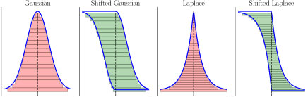
Figure 1: Illustration of the sampling area for different distribution: (shifted) Gaussian and (shifted) Laplace.

Shifted Layered Quantizer. Another approach for leveraging subtractive dithering is based on multishift coupling, as described in Wilson (2000). It is based on the idea of using a sequence of shifted uniform distributions to generate a sequence of target distributions. The key idea is that the sampling from an area $A$ and then projecting onto the $x$-axis is equivalent to the sampling from any horizontal reflection of $A$ and then projecting onto the $x$-axis. Thus, one can can flip one side of a unimodal distribution and still take samples from the part under the flipped side (see Figure 1 with the shifted distributions).

Definition 5.

(Shifted layered quantizer) Given any $Z$ with a unimodal p.d.f. $f_{Z}$, the layered randomized quantizer, producing an error $Z$, is defined using the encoder ${\mathscr{E}}$, the decoder ${\mathscr{D}}$ and randomness $P_{S}$ such that $S=(U,W_{Z})$ with $U\sim\mathcal{U}(0,1)$ independent of $W_{Z}\sim f_{W}$ where the p.d.f. $f_{W}$ is defined through the superlevel sets of $f_{Z}$. For all $x\in\mathbb{R}$ ,

$$f_{W}(x)=\left(b_{Z}^{+}(x)-b_{Z}^{-}(\bar{Z}-x)\right)\mathbf{1}_{\left(0,\bar{Z}\right)}(x),$$

$${\mathscr{E}}(X,S)=\lceil X/f_{W}(W_{Z})+U\rfloor,$$

$${\mathscr{D}}(M,S)=\left(M\!-\!U\right)f_{W}(W_{Z})+\frac{b_{Z}^{+}(W_{Z})+b_{Z}^{-}(\bar{Z}\!-\!W_{Z})}{2}.$$

By construction, the shifted layered quantizer satisfies the AINQ property (see details in Appendix B.1).

3.2 Communication Complexity

To transmit the integer $M$, we should encode it into bits. There are two general approaches. First, if a fixed-length code is used where $M$ is always encoded to the same number of bits, then $\lceil\log|\operatorname{Supp}M|\rceil$ bits are required. Second, if a variable-length code is used, for example, if we encode $M$ using the Huffman code (Huffman, 1952) on the conditional distribution $p_{M|S}$, then we require an expected encoding length bounded between $\operatorname{\mathcal{H}}(M|S)$ and $\operatorname{\mathcal{H}}(M|S)+1$. We will see that the direct layered quantizer gives a better variable-length performance, whereas the shifted layered quantizer gives a better fixed-length performance.

For variable-length codes, it has been shown in (Hegazy and Li, 2022, Theorem 4) that every AINQ scheme with error distribution $f_{Z}$ and uniform input $X\sim\mathcal{U}(0,t)$ must satisfy

$$\operatorname{\mathcal{H}}(M|S)\geq\log(t)+h(D_{Z}),$$ (4)

where $D_{Z}$ is defined in Definition 4, and $-h(D_{Z})$ is called the layered entropy. It has also been shown in Hegazy and Li (2022) that the direct layered quantizer is almost optimal, in the sense that as long as $Z$ has a unimodal distribution and $\operatorname{Supp}(X)\subseteq\left[0,t\right]$, it achieves

$$\operatorname{\mathcal{H}}(M|S)\leq\log(t)+\frac{8\log{(e)}}{t}\sqrt{\operatorname{\mathbb{V}}\left[Z\right]}+h(D_{Z}).$$ (5)

The gap between (4) and (5) tends to $0$ as $t\to\infty$.

While the shifted layered quantizer is not asymptotically optimal, the optimality gap (the gap between the $\operatorname{\mathcal{H}}(M|S)$ attained and its optimal value) is still relatively small as shown below.

Proposition 1.

(Optimality Gap) For a target unimodal noise distribution $f_{Z}$ that is symmetric, the shifted layered quantizer achieves

$$\operatorname{\mathcal{H}}(M|S)\leq\log(t)+\frac{8\log(e)}{t}\sqrt{\operatorname{\mathbb{V}}\left[Z\right]}+h(W_{Z}),$$

and the optimality gap of using the shifted layered quantizer is upper bounded by $(8\log(e)/t)\sqrt{\operatorname{\mathbb{V}}\left[Z\right]}+2$.

Figure 2 below shows the conditional entropy $\operatorname{\mathcal{H}}(M|S)$ needed to simulate a Gaussian noise and a Laplace noise with standard deviation $\sigma\in\{1;3\}$ according to the support size $t$ where $X\sim\mathcal{U}(0,t)$. The gap is smaller than $1$ bit for all the values computed.

The advantage of the shifted layered quantizer is its fixed-length performance. A fixed-length code has the advantage that we do not have to build a Huffman code on the conditional distribution $p_{M|S}$ for each $S$, which may be infeasible. Since the shifted layered quantizer has a quantization step size bounded away from $0$ as shown in Figure 1, it provides a fixed upper bound on the number of quantization bits.

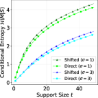
(a) Gaussian error

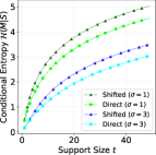
(b) Laplace error

Figure 2: Conditional entropy $\mathcal{H}(M|S)$ of the layered quantizers with Gaussian/Laplace error distribution.

Proposition 2.

(Minimal step size for shifted layered) For a required $f_{Z}$, denote by $\eta_{Z}$ the minimal step size of the shifted layer quantizer, i.e. $\eta_{Z}\coloneqq\min f_{W}$. Assume that the input $X$ lies in a fixed interval of length $t$.
•  If $Z\sim\text{Laplace}(0,\sigma/\sqrt{2})$ then $\eta_{Z}=\sigma\sqrt{2}\ln{2}$ and $\left\lvert\operatorname{Supp}M\right\rvert\leq 2+t/(\sigma\sqrt{2}\ln{2})$.
•  If $Z\sim\mathcal{N}(0,\sigma^{2})$ then $\eta_{Z}=2\sigma\sqrt{\ln 4}$ and
$\left\lvert\operatorname{Supp}M\right\rvert\leq 2+t/(2\sigma\sqrt{\ln 4})$.

4 AGGREGATE MECHANISMS

4.1 Homomorphic Mechanisms

For an individual AINQ mechanism, the descriptions $M_{1},\ldots,M_{n}$ sent from the users must all be available to the server. The descriptions cannot be first aggregated into a single number before decoding. We study aggregate AINQ mechanisms where such “intermediate aggregation” of descriptions is possible.

Definition 6.

(Homomorphic) An aggregate AINQ mechanism is homomorphic if there exists functions $\mathscr{D}:\mathcal{M}\times\mathcal{S}\times\mathcal{T}\to\mathbb{R}^{d}$ (called the homomorphic decoding function) such that the overall decoding function is

$$\overline{\mathscr{D}}(m_{1},s_{1},\ldots,m_{n},s_{n},t)=\frac{1}{n}\mathscr{D}\left(\sum_{i=1}^{n}m_{i},\,\sum_{i=1}^{n}s_{i},\,t\right)$$ (6)

and for all $t$, $\mathscr{D}(\cdot,\cdot,t):\mathcal{M}\times\mathcal{S}\to\mathbb{R}^{d}$ is a homomorphism, i.e., $\mathscr{D}(m,s,t)+\mathscr{D}(m^{\prime},s^{\prime},t)=\mathscr{D}(m+m^{\prime},s+s^{\prime},t)$ for all $m,m^{\prime},s,s^{\prime}$.

Here we require $\mathcal{M}$ and $\mathcal{S}$ to be abelian groups (e.g., $\mathcal{M}=\mathbb{Z}^{d}$, $\mathcal{S}=\mathbb{R}^{d}$) so we can perform addition over $\mathcal{M}$ and $\mathcal{S}$. For a homomorphic scheme, the server only requires the common randomness $(S_{i})_{i},T$ and the sum of the descriptions $\sum_{i=1}^{n}M_{i}$, not the individual descriptions $M_{1},\ldots,M_{n}$.

In federated learning, homomorphic mechanisms have several advantages. First, the descriptions $M_{1},\ldots,M_{n}$ can be passed from the clients to the server through a network for sum computation (Ramamoorthy and Langberg, 2013; Rai and Dey, 2012; Qu et al., 2021; Rizk and Sayed, 2021), resulting in a reduction of communication cost. A simple method is to have each node in the network add all incoming signals and pass the sum to the next node. The internal nodes in the network do not need to access $(S_{i})_{i},T$. Second, homomorphic mechanisms are compatible with SecAgg (Bonawitz et al., 2017) and other additive homomorphic cryptosystems. We can perform SecAgg on $M_{1},\ldots,M_{n}$ so that the server can only know $\sum_{i=1}^{n}M_{i}$, but not the individual $M_{i}$’s so as to preserve privacy.

The layered quantizers of the previous section do not produce homomorphic mechanisms. The reason is that the quantization step sizes of the $n$ users are randomly drawn and different. Thus, the quantized data $M_{i}$’s are at different scales and cannot be added together. A simple and naive way to obtain an homomorphic mechanism is to rely on subtractive dithering (Example 1) with a fixed step size $w$ for each user.

4.2 Irwin-Hall Mechanism

When applying subtractive dithering for each of the $n$ users, the resultant noise of the individual AINQ mechanism follows a scaled Irwin-Hall distribution. More precisely, consider $S=(S_{1},\ldots,S_{n})$ to be an i.i.d. sequence of $\mathcal{U}(-1/2,1/2)$ random variables and $T=0$ to be degenerate. The encoding function is $M_{i}=\mathscr{E}(x_{i},S_{i})=\lceil x_{i}/w+S_{i}\rfloor$ where $w:=2\sigma\sqrt{3n}$, and the decoding function is $Y=w(\sum_{i}M_{i}-\sum_{i}S_{i})$. The noise is a scaled Irwin-Hall distribution $\mathrm{IH}(n,0,\sigma^{2})$, where $\mathrm{IH}(n,\mu,\sigma^{2})$ denotes the distribution of $n^{-1}\sum_{i=1}^{n}Z_{i}+\mu$ with $Z_{1},\ldots,Z_{n}\stackrel{{\scriptstyle iid}}{{\sim}}\mathcal{U}(-\sigma\sqrt{3n},\,\sigma\sqrt{3n})$. Note that $\mathrm{IH}(n,0,\sigma^{2})$ has mean $0$ and variance $\sigma^{2}$, and approximates the Gaussian distribution $\mathcal{N}(0,\sigma^{2})$ when $n$ is large. We call this the Irwin-Hall mechanism.

While this mechanism is simple and homomorphic (the decoding function only depends on $\sum_{i}M_{i}$ and $\sum_{i}S_{i}$), an obvious downside is that the resultant noise distribution is the Irwin-Hall distribution, not the Gaussian distribution. The Irwin-Hall distribution itself is not a privacy-preserving noise for $(\varepsilon,\delta)$-differential privacy nor Rényi privacy. Moreover, specific FL applications such as stochastic Langevin dynamics (Welling and Teh, 2011; Vono et al., 2022) or randomized smoothing (Duchi et al., 2012; Scaman et al., 2018) specifically require a Gaussian distribution. This motivates the development of advanced aggregate AINQ mechanisms.

4.3 Aggregate $Q$ Mechanism

Let $P=\mathrm{IH}(n,0,\sigma^{2})$ be the Irwin-Hall distribution. We have seen in Section 4.2 that the Irwin-Hall mechanism produces a noise with distribution $P$. The idea is now to decompose the desired noise distribution $Q$ (e.g. Gaussian) into a mixture of shifted and scaled versions of $P$ in the form “$aP+b$”, use the global common randomness $T$ to select the shifting and scaling factors according to the mixture probabilities, and perform the Irwin-Hall mechanism with the input and output shifted and scaled. In this section, we construct a homomorphic aggregate AINQ mechanism with a noise distribution $Q$, called the aggregate $Q$ mechanism, using this strategy.

Definition 7.

(Mixture set) For probability distributions $P,Q$, denote by $\Pi_{A,B}(P,Q)$ the set of joint probability distributions $\pi_{A,B}$ of the random variables $A\in\mathbb{R}$ and $B\in\mathbb{R}$ such that if $(A,B)\sim\pi_{A,B}$ is independent of $Z\sim P$, then $AZ+B\sim Q$.

Definition 8.

(Aggregate $Q$ mechanism) Let $S_{1},\ldots,S_{n}\stackrel{{\scriptstyle iid}}{{\sim}}\mathcal{U}(-1/2,1/2)$ and $T=(A,B)\sim\pi_{A,B}\in\Pi_{A,B}(P,Q)$. The aggregate $Q$ mechanism is defined by $w:=2\sigma\sqrt{3n}$ and

$$\mathscr{E}(x,s,a,b):=\left\lceil x/(aw)+s\right\rfloor,$$

$$\overline{\mathscr{D}}((m_{i})_{i},(s_{i})_{i},a,b):=\frac{aw}{n}\left(\sum_{i=1}^{n}m_{i}-\sum_{i=1}^{n}s_{i}\right)+b.$$

Basically, we generate $A,B$ randomly, and then run the Irwin-Hall mechanism scaled by $A$ and shifted by $B$. The resultant noise distribution is $Q$ as precised in the next Proposition.

Proposition 3.

The aggregate mechanism of Def.8 satisfies the AINQ property with noise distribution $Q$, and is homomorphic.

4.4 Aggregate Gaussian Mechanism

We now study the case where $Q$ is the Gaussian distribution, and describe the construction of $\pi_{A,B}$ which decomposes $Q$ into a mixture of Irwin-Hall distributions. We call this the aggregate Gaussian mechanism.

Step 1. First, we study how to decompose $\mathcal{U}(-1/2,1/2)$ (instead of $Q$) into a mixture of shifted and scaled versions of the Irwin-Hall distribution $P$ with a pdf $f$. Assume $f$ is appropriately scaled so its support is $[-1/2,1/2]$. For $-1/2\leq x\leq 1/2$, decompose $\mathcal{U}(-1/2,1/2)$ into the mixture $(1/f(0))f(x)+(1-1/f(0))\varphi(x)$ where $\varphi(x)=(f(0)-f(x))/(f(0)-1)$ is a bimodal distribution with modes $\{-1/2;1/2\}$, and can be decomposed into uniform distributions using the strategy in Section 3.1. These uniform distributions can be recursively decomposed into a mixture of a shifted/scaled $f$ and other uniform distributions, and so on. See Figure 3, and Algorithm DecomposeUnif in Appendix A.2.

Step 2. To decompose the Gaussian distribution $Q$ with a pdf $g$, we first decompose $g$ into the mixture $g(x)=\lambda f(x)+(1-\lambda)\psi(x)$ where $\lambda$ is as large as possible such that $\psi$ is still unimodal. A practical choice is $\lambda=\inf_{x>0}\mathrm{d}g(x)/\mathrm{d}f(x)$ if $n\geq 3$, and $\lambda=0$ if $n\leq 2$. We then decompose $\psi$ into a mixture of uniform distributions, using the strategy in Section 3.1, and decompose those uniform distributions using the aforementioned strategy. Refer to Figure 3, and Algorithm Decompose in Appendix A.4.

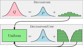
Figure 3: Decomposition of $Q$ into a mixture of scaled Irwin-Hall $P$. Algorithm Decompose decomposes $Q$ into a mixture of $P$ and a unimodal distribution, where the latter is then decomposed into a mixture of uniform distributions and passed to DecomposeUnif.

4.5 Theoretical Analysis

We now study the communication cost. Assuming the data $x_{i}$ is bounded by $|x_{i}|\leq t/2$ for $i=1,\ldots,n$, we have $|\mathscr{E}(x_{i},S_{i},A,B)|\leq\left\lceil t/(2w|A|)\right\rceil$. Therefore, $M_{i}$ can be encoded into $\lceil\log(t/(w|A|)+3)\rceil$ bits conditional on $A$. The expected amount of communication per client is upper-bounded by $\mathbb{E}(\lceil\log(t/(w|A|)+3)\rceil)$ which is approximately equal to $\mathbb{E}[-\log|A|]+\log(t/(2\sigma\sqrt{3n}))$ bits. Hence, we can construct an aggregate AINQ mechanism with a small amount of communication if we have a small $\mathbb{E}[-\log|A|]$. To study this quantity, we introduce a notion called relative mixture entropy.

Definition 9 (Relative mixture entropy).

Given probability distributions $P,Q$ over $\mathbb{R}$, the relative mixture entropy is $h_{\mathrm{M}}(Q\|P):=\sup_{\Pi_{A,B}(P,Q)}\mathbb{E}_{\Pi_{A,B}}[\log|A|]$ where the supremum is over $\Pi_{A,B}(P,Q)$.

Relative mixture entropy has several desirable properties similar to the differential entropy (see Appendix A.1). In particular, $h_{\mathrm{M}}(Q\|P)\leq h(Q)-h(P)$ can be upper-bounded in terms of the difference of differential entropies. We have the following bound on the communication cost in terms of $h_{\mathrm{M}}(Q\|P)$.

Theorem 1.

(Complexity) Let $P=\mathrm{IH}(n,0,\sigma^{2})$ be an Irwin-Hall distribution. Assume $|x_{i}|\leq t/2$ for $i=1,\ldots,n$. There exists an aggregate AINQ mechanism for simulating a noise distribution $Q$, with an expected amount of communication per client upper-bounded by

$$-h_{\mathrm{M}}(Q\|P)+\log\frac{t}{2\sigma\sqrt{3n}}+\frac{6\sigma\sqrt{3n}\log e}{t}\cdot\frac{\mathbb{E}_{Z\sim Q}[|Z|]}{\mathbb{E}_{Z\sim P}[|Z|]}+1.$$

To give an upper bound on the expected communication cost, it remains to give a lower bound on $h_{\mathrm{M}}(Q\|P)$.

Theorem 2.

(Lower bound) For two distributions $P,Q$ with pdfs $f,g$, respectively, that are unimodal, differentiable and symmetric around $0$ with $L:=2\sup\{x:f(x)>0\}<\infty$ and $\lambda:=\inf_{x>0}\mathrm{d}g(x)/\mathrm{d}f(x)$, we have

$$h_{\mathrm{M}}(Q\|P)\geq-(1\!-\!\lambda)\!\left(Lf(0)+\log\frac{eL(g(0)-\lambda f(0))}{2(1-\lambda)}\right)\!.$$

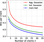
(a) $t=64$

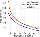
(b) $t=2048$

Figure 4: Comparison between the aggregated Gaussian, individual Gaussian (direct) and Irwin-Hall mechanisms, $\sigma=1$, (a) $x_{i}\in[-2^{5};2^{5}]$, (b) $x_{i}\in[-2^{10};2^{10}]$.

We can then combine Theorems 1, 2 to give a bound on the communication cost of the aggregate Gaussian mechanism. The proofs of the theorems are given in Appendix B.6 and B.7. The pseudocode is given in Algorithms Encode and Decode in Appendix A.5. Figure 4 compares the communication cost per client of the aggregate Gaussian mechanism, individual Gaussian mechanism (direct layered quantizer) and Irwin-Hall mechanism where the bounds are computed using Theorem 1 and Theorem 2. We can see that the aggregate Gaussian mechanism can have a smaller communication cost than the individual Gaussian mechanism for a large number of clients, though not as small as the Irwin-Hall mechanism. We also remark that aggregate Gaussian is homomorphic (unlike individual Gaussian), and has a noise distribution that is exactly Gaussian (unlike the Irwin-Hall mechanism).

5 COMPRESSION AND SUBSAMPLING FOR PRIVACY

5.1 Trusted server with subsampling strategy

Subsampling (Li et al., 2012; Balle et al., 2018) is a technique for enhancing privacy, where only a subset of clients or their data is selected for transmission. It can be leveraged to reduce communication cost while improving DP guarantees. Recently, (Chen et al., 2023) introduced coordinate-wise subsampling to derive DP schemes with optimal communication utility tradeoffs. We now describe how this scheme can be improved with an AINQ mechanism.

We are interested in the subsampled individual Gaussian mechanism (SIGM) with shifted layered quantizer. First consider the case in dimension $d=1$ with $n$ clients and sampling variables $B_{1},\ldots,B_{n}\sim\mathcal{B}(\gamma)$ ($\gamma\in[0,1]$), where $B_{i}=1$ if client $i$ is selected and $B_{i}=0$ otherwise. Let $\tilde{n}=\sum_{i}B_{i}$ be the number of selected clients and let $\mathscr{E},\mathscr{D}$ be the encoding and decoding functions in Def.5 for the noise distribution $\mathcal{N}(0,(\sigma\gamma n)^{2})$. The mechanism works as follows: (1) generate the global shared randomness $B_{1},\ldots,B_{n}\sim\mathcal{B}(\gamma)$; (2) generate the shared randomness $S_{i}$ if $B_{i}=1$; (3) client $i$ sends $M_{i}=\mathscr{E}(x_{i}\sqrt{\tilde{n}},S_{i})$ if $B_{i}=1$, or $M_{i}=0$ if $B_{i}=0$; and (4) server outputs $Y=(\gamma n\sqrt{\tilde{n}})^{-1}\sum_{i:\,B_{i}=1}\mathscr{D}(M_{i},S_{i})$. It can be checked that $Y-(\gamma n)^{-1}\sum_{i:B_{i}=1}x_{i}\sim\mathcal{N}(0,\sigma^{2})$. The proof, the generalization to $d$ dimensional data, and the algorithm are included in Appendix A.6. This mechanism achieves the same statistical behavior as CGSM (Chen et al., 2023), with the benefit that it directly ensures an exact Gaussian noise through quantization without the need to first incur a compression error independently of DP noise. Invoking (Chen et al., 2023, Theorem 4.1) and Prop. 2, we have the following result.

Proposition 4.

If $x_{1},\ldots,x_{n}\in[-c,c]^{d}$, then SIGM is $(\varepsilon,\delta)$-DP with a noise level of order

$$\sigma^{2}=\Theta\bigg{(}\frac{c^{2}\ln(1/\delta)}{n^{2}\gamma^{2}}+\frac{c^{2}d(\ln(d/\delta)+\varepsilon)\ln(d/\delta)}{n^{2}\varepsilon^{2}}\bigg{)},$$

where the cost per client is $\mathcal{O}\left(\gamma d\log(2+c/(\sigma\sqrt{n\gamma}))\right)$, and the error $\operatorname{\mathbb{E}}[\left\lVert Y-n^{-1}\sum_{i}x_{i}\right\rVert^{2}_{2}]$ is at most $\frac{dc^{2}}{n\gamma}+d\sigma^{2}$.

Remark 1.

(Flattening and geometry) To extend this result for data bounded in $\ell_{2}$ norm, one may rely on flattening techniques to convert the $\ell_{2}$ geometry into an $\ell_{\infty}$ geometry and obtain tighter utility analysis. Using Kashin’s representation as in Chen et al. (2023) or some Walsh-Hadamard/Fourier transform as in Kairouz et al. (2021a), the SIGM mechanism enjoys the optimal utility bound of order $\mathcal{O}(d/(n^{2}\varepsilon^{2}))$. Observe that these flattening schemes require $\mathcal{O}(d^{2})$ or $\mathcal{O}(d\log d)$ depending on the operation.

Quantized Aggregation Scheme	$\begin{array}[]{c}\text{Homo-}\\ \text{morphic}\end{array}$	$\begin{array}[]{c}\text{Gaussian}\\ \text{noise}\end{array}$	$\begin{array}[]{c}\text{R\'{e}nyi}\\ \text{DP}\end{array}$	$\begin{array}[]{c}\text{Fixed}\\ \text{length}\end{array}$
Individual - Direct (Def.4)	$\times$	$\checkmark$	$\checkmark$	$\times$
Individual - Shifted (Def.5)	$\times$	$\checkmark$	$\checkmark$	$\checkmark$
Irwin-Hall (Section 4.2)	$\checkmark$	$\times$	$\times$	$\checkmark$
Aggregate Gaussian (Def.8)	$\checkmark$	$\checkmark$	$\checkmark$	$\times$
Subsampled ind. Gaussian (Sec. 5)	$\times$	$\checkmark$	$\checkmark$	$\checkmark$

Table 1: Comparison of aggregate AINQ mechanisms – whether they are homomorphic, can produce a Gaussian noise, achieve Rényi DP, and have a fixed number of communication bits used.

Numerical comparison. We empirically evaluate our distributed mean estimation scheme SIGM with the method CSGM in a similar framework as in Chen et al. (2023). The parameter configuration is: number of clients $n\in\{1000;2000\}$, dimension $d\in\{100;500\}$, probability of information accidentally being leaked $\delta=10^{-5}$, privacy budget $\varepsilon\in[0.5;4]$ and subsampling parameter $\gamma\in\{0.3;0.5;1.0\}$. Figure 5 displays the mean squared errors (MSE) obtained over $100$ independent runs. The number of bits used by CSGM is kept equal to the number of bits used by SIGM. For the same $\varepsilon$, $\gamma$ and the number of bits used, SIGM allows a smaller MSE compared to the CSGM.

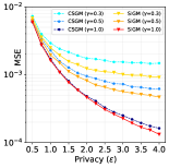
(a) $n=1000,\ d=100$

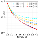
(b) $n=2000,\ d=500$

Figure 5: Mean Squared Error for CSGM and SIGM.

5.2 Less-trusted with SecAgg

The Distributed Discrete Gaussian (DDG) mechanism (Kairouz et al., 2021a) can leverage SecAgg to achieve differential privacy guarantees against the server, which is a stronger setting than that of the less-trusted server. However, in practical implementation, it often requires a much higher number of bits per coordinate.

We adapt the experiments from Kairouz et al. (2021a) which show the utility of the DDG mechanism with different number of bits against the standard Gaussian mechanism. On the other hand, using Elias gamma coding, we calculate the number of bits needed for the aggregate Gaussian mechanism and the individual mechanism using shifted layered quantizer to match a Gaussian mechanism. The results of Figure 6 are obtained over $30$ runs with $n=500$ and $d=75$ and highlight the great performance of aggregate Gaussian. While DDG offers stronger privacy guarantees, i.e., DP against the server, it comes at a heavy cost in terms of bits in comparison to aggregate Gaussian, which is also compatible with SecAgg.

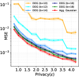
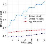
Figure 6: MSE (left) and bits per client (right) against $\varepsilon$. The DDG mechanism can require up to $b=18$ bits to match the privacy-utility tradeoff of aggregate Gaussian, where the latter only requires $\leq 2.5$ bits on average. We also plot the bits per client for shifted layered quantizer (using a fixed or variable-length code) on the right figure for comparison (we remark that shifted layered quantizer is incompatible with SecAgg).

Appendix A Additional results on aggregated mechanisms

A.1 Properties of relative mixture entropy

Proposition 5.

The relative mixture entropy satisfies:

1. (Shifting and scaling) Let $X,Y$ be random variables, and denote the distribution of $X$ as $P_{X}$. For constants $a,c\neq 0$ and $b,d\in\mathbb{R}$,

   $$h_{\mathrm{M}}(P_{cY+d}\|P_{aX+b})=h_{\mathrm{M}}(P_{Y}\|P_{X})+\log\frac{|c|}{|a|}.$$

2. (Concavity in $Q$) For a fixed $P$, $h_{\mathrm{M}}(Q\|P)$ is concave in $Q$.

3. (Chain rule) For distributions $P,Q,R$,

   $$h_{\mathrm{M}}(R\|P)\geq h_{\mathrm{M}}(R\|Q)+h_{\mathrm{M}}(Q\|P).$$

4. (Bound via differential entropy) If $P,Q$ are continuous distributions,

   $$h_{\mathrm{M}}(Q\|P)\leq h(Q)-h(P),$$

   where $h(P)$ is the differential entropy of $P$.

Proof.

Property (1) is straightforward. To show concavity (2), consider $\lambda\in[0,1]$ and two distributions $Q_{1},Q_{2}$, and consider $(A_{1},B_{1})$ independent of $(A_{2},B_{2})$ independent of $Z\sim P$ such that $A_{1}Z+B_{1}\sim Q_{1}$, $A_{2}Z+B_{2}\sim Q_{2}$. Take $(A,B)=(A_{1},B_{1})$ with probability $\lambda$, and $(A,B)=(A_{2},B_{2})$ with probability $1-\lambda$. We have

$$AZ+B\sim\lambda Q_{1}+(1-\lambda)Q_{2},\qquad\mathbb{E}[\log|A|]=\lambda\mathbb{E}[\log|A_{1}|]+(1-\lambda)\mathbb{E}[\log|A_{2}|].$$

Taking supremum gives us the desired result. To show the chain rule (3), consider $(A_{1},B_{1})$ independent of $(A_{2},B_{2})$ independent of $Z\sim P$ such that $Y=A_{1}Z+B_{1}\sim Q$, and $A_{2}Y+B_{2}\sim R$. We have $A_{1}A_{2}Z+A_{2}B_{1}+B_{2}\sim R$, and $\mathbb{E}[\log|A_{1}A_{2}|]=\mathbb{E}[\log|A_{1}|]+\mathbb{E}[\log|A_{2}|]$. Taking supremum gives us the desired result. To show the bound via differential entropy (4), if $(A,B)$ is independent of $Z\sim P$, then $AZ+B\sim Q$ and

$$h(Q)=h(AZ+B)\geq h(AZ+B\,|\,A,B)=h(Z)+\mathbb{E}[\log|A|].$$

∎

A.2 Algorithm DecomposeUnif

As an intermediate step, we study how we can simulate $\mathcal{U}(-1/2,1/2)$ using a noise with p.d.f. function $f$ that is unimodal, symmetric around $0$, and supported over $[-1/2,1/2]$ (e.g. a scaled version of Irwin-Hall). The idea is to recursively express uniform distributions as mixtures of shifted and scaled versions of $f$ and other uniform distributions, and repeat ad infinitum.

We now describe the operation of decomposing $\mathcal{U}(-1/2,1/2)$ into a mixture of shifted and scaled versions of $f(x)$. For the sake of simplicity, assume $f(x)$ is unimodal, symmetric around $0$, and supported over $[-1/2,1/2]$ (e.g. a scaled version of Irwin-Hall). First, we can express the uniform distribution $\mathcal{U}(-1/2,1/2)$ as a mixture of $f(x)$ and other uniform distributions as follows. Generate $U\sim\mathcal{U}(-1/2,1/2)$ independent of $V\sim\mathcal{U}(0,1)$. If $V\leq f(U)/f(0)$, then generate $X\sim f$. If $V>f(U)/f(0)$ and $U>0$, then take $S=f^{-1}(Vf(0))$ (where $f^{-1}(y):=\inf\{x\geq 0:\,f(x)\leq y\}$), and generate $X\sim\mathcal{U}(S,1/2)$. If $V>f(U)/f(0)$ and $U<0$, then take $S=f^{-1}(Vf(0))$, $X\sim\mathcal{U}(-1/2,-S)$. Then we can show that $X\sim\mathcal{U}(-1/2,1/2)$. We can then recursively express these uniform distributions in the mixture as mixtures of shifted and scaled versions of $f(x)$ and other uniform distributions, and repeat ad infinitum.

Algorithm DecomposeUnif takes $f$ and a random number generator $\mathfrak{P}$ as input (where we can invoke $\mathfrak{P}()$ to obtain a $\mathcal{U}(0,1)$ random number), and outputs two random variables $A,B$ such that if we generate $X\sim f$, then $AX+B\sim\mathcal{U}(-1/2,1/2)$.

    Input: pdf $f$, random number generator $\mathfrak{P}$

    Output: scale $a\in(0,\infty)$ and shift $b\in\mathbb{R}$

1:$a\leftarrow 1$, $b\leftarrow 0$

2:while True do

3:     $u\leftarrow\mathfrak{P}()-1/2$

4:     $v\leftarrow\mathfrak{P}()$

5:     if  $v\leq f(u)/f(0)$ then

6:         return $(a,b)$

7:     else

8:         $s\leftarrow f^{-1}(vf(0))$

9:         $b\leftarrow b+a\cdot\mathrm{sgn}(u)\left(\frac{s+1/2}{2}\right)$

10:         $a\leftarrow a(1/2-s)$

11:     end if

12:end while

Algorithm 1 $\textsc{DecomposeUnif}(f,\mathfrak{P})$

A.3 Theoretical analysis of Algorithm DecomposeUnif

We now analyze the value of $\mathbb{E}[\log A]$ given by Algorithm DecomposeUnif, which will give a bound on $h_{\mathrm{M}}(\mathcal{U}(-1/2,1/2)\|P)$. We invoke the following result which follows from (Hegazy and Li, 2022, Theorem 1).

Theorem 3.

For any probability density function $f$, we have

$$h_{\mathrm{M}}(f\,\|\,\mathcal{U}(-1/2,1/2))\leq h_{\mathrm{L}}(f)$$

and equality holds if $f$ is a unimodal distribution with a finite mean, where $h_{\mathrm{L}}(f):=\int_{0}^{\infty}\lambda(L_{\tau}^{+}(f))\log\lambda(L_{\tau}^{+}(f))\mathrm{d}\tau$ is called the layered entropy of $f$, where $L_{\tau}^{+}(f):=\{x\in\mathbb{R}:\,f(x)\geq\tau\}$ is the superlevel set, and $\lambda(L_{\tau}^{+}(f))$ is the Lebesgue measure.

If $(X,Y)\sim\mathcal{U}\{(x,y):\,0\leq y\leq f(x)\}$, then $h_{\mathrm{L}}(f)=-h(Y)$ (Hegazy and Li, 2022). Therefore, $h_{\mathrm{L}}(f)\geq-\log\sup_{x\in\mathbb{R}}f(x)$ is lower bounded by the differential min-entropy of $f$. We have the following bound.

Corollary 1.

For any unimodal p.d.f. $f$ with a finite mean: $h_{\mathrm{M}}(f\,\|\,\mathcal{U}(-1/2,1/2)\geq-\log\sup_{x\in\mathbb{R}}f(x)$.

We can now bound $h_{\mathrm{M}}(\mathcal{U}(-1/2,1/2)\|P)$. The following lemma will be useful in the proof of Theorem 2.

Lemma 1.

For any unimodal probability density function $f$ with $f^{*}:=\sup_{x}f(x)$, with a bounded support $L:=\sup\{x:f(x)>0\}-\inf\{x:f(x)>0\}$, we have $h_{\mathrm{M}}(\mathcal{U}(-1/2;1/2)\,\|\,f)\geq-Lf^{*}-\log(eL/2).$

Proof.

Write $\mathrm{U}:=\mathrm{Unif}(-1/2,1/2)$. By the shifting and scaling property in Proposition 5, we can assume $L=1$ and $f$ is supported over $[-1/2,1/2]$ without loss of generality. Assume the maximum of $f$ is attained at $x_{0}$. We can express $\mathrm{Unif}(-1/2,1/2)$ as a mixture

$$\frac{1}{f^{*}}f(x)+\nu_{1}g_{1}(x)+\nu_{2}g_{2}(x),\quad\text{ where }\nu_{1}:=\int_{-1/2}^{x_{0}}\left(1-\frac{f(x)}{f^{*}}\right)\mathrm{d}x,\;\;\;\nu_{2}:=\int_{x_{0}}^{1/2}\left(1-\frac{f(x)}{f^{*}}\right)\mathrm{d}x,$$

and

$$g_{1}(x):=\frac{1-f(x)/f^{*}}{\nu_{1}}\;\;\text{for}\;-\frac{1}{2}\leq x\leq x_{0},\;\;\;g_{2}(x):=\frac{1-f(x)/f^{*}}{\nu_{2}}\;\;\text{for}\;x_{0}\leq x\leq\frac{1}{2}.$$

Note that both $g_{1}(x)$ and $g_{2}(x)$ are unimodal, and $\nu_{1}+\nu_{2}=1-1/f^{*}$. We have

$$h_{\mathrm{M}}(\mathrm{U}\|f) \stackrel{{\scriptstyle(a)}}{{\geq}}\nu_{1}h_{\mathrm{M}}(g_{1}\|f)+\nu_{2}h_{\mathrm{M}}(g_{2}\|f)$$

$$\stackrel{{\scriptstyle(b)}}{{\geq}}\nu_{1}\left(h_{\mathrm{M}}(g_{1}\|\mathrm{U})+h_{\mathrm{M}}(\mathrm{U}\|f)\right)+\nu_{2}\left(h_{\mathrm{M}}(g_{2}\|\mathrm{U})+h_{\mathrm{M}}(\mathrm{U}\|f)\right)$$

$$=\nu_{1}h_{\mathrm{M}}(g_{1}\|\mathrm{U})+\nu_{2}h_{\mathrm{M}}(g_{2}\|\mathrm{U})+\left(1-\frac{1}{f^{*}}\right)h_{\mathrm{M}}(\mathrm{U}\|f).$$

where (a) is by concavity, and (b) is by the chain rule (Proposition 5). Hence,

$$h_{\mathrm{M}}(\mathrm{U}\|f) \geq f^{*}\nu_{1}h_{\mathrm{M}}(g_{1}\|\mathrm{U})+f^{*}\nu_{2}h_{\mathrm{M}}(g_{2}\|\mathrm{U})$$

$$\stackrel{{\scriptstyle(c)}}{{\geq}}f^{*}\nu_{1}\log\nu_{1}+f^{*}\nu_{2}\log\nu_{2}$$

$$\geq f^{*}2\left(\frac{1-1/f^{*}}{2}\right)\log\frac{1-1/f^{*}}{2}$$

$$=(f^{*}-1)\log\frac{f^{*}-1}{2f^{*}}$$

$$=-(f^{*}-1)-(f^{*}-1)\log\left(1+\frac{1}{f^{*}-1}\right)$$

$$\geq-(f^{*}-1)-(f^{*}-1)\frac{\log e}{f^{*}-1}$$

$$=-f^{*}-\log\frac{e}{2},$$

where (c) is by Corollary 1. ∎

A.4 Algorithm Decompose

The goal is to simulate an additive noise channel with a noise p.d.f. $g$ that is unimodal, symmetric around $0$ and differentiable knowing that we can simulate an additive noise channel with a noise p.d.f. $f$ with same properties. The naive and quite inefficient way is to decompose $g$ into a mixture of uniform distributions, and run the DecomposeUnif algorithm on those uniform distributions. Instead, we first decompose $g$ into the mixture

$$g(x)=\lambda f(x)+(1-\lambda)\psi(x)$$

where $\lambda$ is as large as possible such that $\psi$ is still unimodal. A practical choice is $\lambda=\inf_{x>0}\mathrm{d}g(x)/\mathrm{d}f(x)$ if $n\geq 3$, and $\lambda=0$ if $n\leq 2$. We then decompose $\psi$ into a mixture of uniform distributions, and run DecomposeUnif. Algorithm Decompose below computes the decomposition of $g$ into a mixture of shifted and scaled versions of $f$. It takes $f,g$ and a random number generator $\mathfrak{P}$ as input, and outputs two random variables $A,B$ such that if we generate $X\sim f$, then $AX+B\sim g$.

    Input: pdfs $f,g$, random number generator $\mathfrak{P}$

    Output: scale $a\in(0,\infty)$ and shift $b\in\mathbb{R}$

1:$\lambda\leftarrow\inf_{x>0}\frac{\mathrm{d}g(x)}{\mathrm{d}f(x)}$

2:Sample $x\sim g$ using $\mathfrak{P}$

3:$v\leftarrow g(x)\cdot\mathfrak{P}()$

4:if  $v>g(x)-\lambda f(x)$ then

5:     return $(1,0)$

6:else

7:     $s\leftarrow\sup\{x^{\prime}\geq 0:\,v\leq g(x^{\prime})-\lambda f(x^{\prime})\}$

8:     $L\leftarrow 2\sup\{x:f(x)>0\}$

9:     $\tilde{f}\leftarrow(x\mapsto f(x/L)/L)$ (support of $\tilde{f}$ is $[-1/2,1/2]$)

10:     $(a,b)\leftarrow\textsc{DecomposeUnif}(\tilde{f},\mathfrak{P})$

11:     return $(2as/L,\,2bs)$

12:end if

Algorithm 2 $\textsc{Decompose}(f,g,\mathfrak{P})$

A.5 Algorithms for Aggregate Gaussian Mechanism

We describe the encoding and decoding algorithms for the aggregate Gaussian mechanism. We assume the server and all the clients share a common random seed, which they use to initialize their pseudorandom number generators (PRNG) $\mathfrak{P}$. Since each PRNG is initialized with the same seed, they are guaranteed to produce the same common randomness $(S_{i})_{i},A,B$ at the clients and server.

1:Input: data $x\in\mathbb{R}$, number of clients $n$, client id $i$, standard deviation $\sigma$, RNG $\mathfrak{P}$

2:Output: description $m\in\mathbb{Z}$

3:$(a,b)\leftarrow\textsc{Decompose}(\mathrm{IH}(n,0,1),\mathcal{N}(0,1),\mathfrak{P})$

4:for $j=1,\ldots,n$ do

5:     $s_{j}\leftarrow\mathfrak{P}()-1/2$

6:end for

7:$w\leftarrow 2\sigma\sqrt{3n}$

8:return $\left\lceil\frac{x}{aw}+s_{i}\right\rfloor$

Algorithm 3 $\textsc{Encode}(x,n,i,\sigma,\mathfrak{P})$

1:Input: sum of descriptions $\Sigma_{m}=\sum_{i=1}^{n}m_{i}\in\mathbb{Z}$, number of clients $n$, standard deviation $\sigma$, RNG $\mathfrak{P}$

2:Output: estimated mean $y\in\mathbb{R}$

3:$(a,b)\leftarrow\textsc{Decompose}(\mathrm{IH}(n,0,1),\mathcal{N}(0,1),\mathfrak{P})$

4:for $j=1,\ldots,n$ do

5:     $s_{j}\leftarrow\mathfrak{P}()-1/2$

6:end for

7:$w\leftarrow 2\sigma\sqrt{3n}$

8:return $\frac{aw}{n}\left(\Sigma_{m}-\sum_{i=1}^{n}s_{i}\right)+b\sigma$

Algorithm 4 $\textsc{Decode}(\Sigma_{m},n,\sigma,\mathfrak{P})$

A.6 Algorithm SIGM for Differential Privacy Applications

Condition on any $B_{1},\ldots,B_{n}$. Definition 5 ensures that $\mathscr{D}(M_{i},S_{i})-x_{i}\sqrt{\tilde{n}}\sim\mathcal{N}(0,(\sigma\gamma n)^{2})$. Therefore

$$Y-(\gamma n)^{-1}\sum_{i:B_{i}=1}x_{i} =(\gamma n\sqrt{\tilde{n}})^{-1}\sum_{i:\,B_{i}=1}\Big{(}\mathscr{D}(M_{i},S_{i})-x_{i}\sqrt{\tilde{n}}\Big{)}$$

$$\sim\mathcal{N}\Big{(}0,(\sigma\gamma n)^{2}(\gamma n\sqrt{\tilde{n}})^{-2}\tilde{n}\Big{)}\;=\;\mathcal{N}(0,\sigma^{2}).$$

To generalize to $d$ dimensional data $x_{1},\ldots,x_{n}\in\mathbb{R}^{d}$, we can simply apply SIGM on each coordinate individually. Note that each coordinate $j\in[d]$ has $B_{1}(j),\ldots,B_{n}(j)$ sampled independently, indicating whether client $i=1,\ldots,n$ should send the coordinate $x_{i}(j)$, similar to the coordinate subsampling strategy in (Chen et al., 2023). The algorithm is given below.

Algorithm 5 Subsampled Individual Gaussian Mechanism (SIGM)

Parameters: Noise variance $\sigma^{2}>0$, Subsampling Bernoulli parameter $\gamma\in[0,1]$

(Shared Randomness)

$B_{1},\ldots,B_{n}\in\left\{0,1\right\}^{d}$ with $B_{i}(j)\sim\mathcal{B}(\gamma)$

$S_{1},\ldots,S_{n}:$ $S_{i}(1,j)\sim\mathcal{U}\left(0,1\right),S_{i}(2,j)\sim W_{\mathcal{N}(0,(\sigma\gamma n)^{2})}$

$\tilde{n}(j)\leftarrow\sum_{i=1}^{n}B_{i}(j)$     for $j\in[d]$

(Client side)

input: private $x_{i}\in\mathbb{R}^{d}$ with $\|x_{i}\|_{2}\leq c$

Encode: For $j\in[d]$

      If $B_{i}(j)=1$ then $M_{i}(j)\leftarrow{\mathscr{E}}({x}_{i}(j)\sqrt{\tilde{n}(j)},S_{i}(\cdot\;,j))$

      else $M_{i}(j)\leftarrow 0$

Send: $M_{i}$ to the server

(Server side)

input: $M_{1},\ldots,M_{n}\in\mathbb{Z}^{d}$

Decode: For $j\in[d]$

      ${\bar{\mu}}(j)\leftarrow(\gamma n\sqrt{\tilde{n}})^{-1}\sum_{i:\,B_{i}(j)=1}\mathscr{D}(M_{i}(j),S_{i}(\cdot,j))$

Return: $\bar{\mu}$

Appendix B Proofs of technical results

B.1 Shifted Layered Quantizer satisfies AINQ

Let us show that the shifted layered quantizer yields the same distribution of error scheme as the direct layered quantizer (Definition 4). Let $\Delta=Y-X$, then $\Delta|V\sim\mathcal{U}\left(b^{-}_{Z}(\bar{Z}-V),b^{+}_{Z}(V)\right)$. Denote $\mathcal{M}=\operatorname{argmax}f_{Z}(x)$ and $m=\text{median}(\mathcal{M})$. It follows that

$$f_{\Delta}(x) =\int_{\mathbb{R}}\frac{\mathbf{1}{\left\{x\in\left(b^{-}_{Z}(\bar{Z}-v),b^{+}_{Z}(v)\right)\right\}}}{W_{Z}(v)}W_{Z}(v)dv$$

$$\stackrel{{\scriptstyle(a)}}{{=}}\int_{\mathbb{R}}\mathbf{1}{\left\{x\in\left(b^{-}_{Z}(\bar{Z}-v),m\right)\right\}}dv+\int_{\mathbb{R}}\mathbf{1}{\left\{x\in\left(m,b_{Z}^{+}(v)\right)\right\}}dv$$

$$\stackrel{{\scriptstyle(b)}}{{=}}\int_{\mathbb{R}}\mathbf{1}{\left\{x\in\left(b_{Z}^{-}(v),m\right)\right\}}dv+\int_{\mathbb{R}}\mathbf{1}{\left\{x\in\left(m,b_{Z}^{+}(v)\right)\right\}}dv$$

$$=\int_{\mathbb{R}}\mathbf{1}{\left\{x\in\left(b_{Z}^{-}(v),b_{Z}^{+}(v)\right)\right\}}dv$$

$$\stackrel{{\scriptstyle(c)}}{{=}}\int_{\mathbb{R}}\mathbf{1}{\left\{x\in\mathcal{L}_{v}(f_{Z})\right\}}dv=f_{Z}(x)$$

where $(a)$ is due to the fact that $m\in\mathcal{L}_{\tau}(f_{Z})$ for any $\tau$, $(b)$ by the change of variable $v=\bar{Z}-v$, and $(c)$ by unimodality of $f_{Z}$.

B.2 Proof of Proposition 1

The conditional entropy $\operatorname{\mathcal{H}}(M_{s}|S_{s})$ may be decomposed as follows

$$\operatorname{\mathcal{H}}(M_{s}|S_{s})-\log(t) =-\log(t)+\int_{0}^{1}\int_{0}^{\bar{Z}}\operatorname{\mathcal{H}}(M_{s}|S_{s}=(u,\tau))f_{W}(\tau)\mathrm{d}\tau\mathrm{d}s$$

$$\leq-\log(t)+\int_{0}^{1}\int_{0}^{\bar{Z}}\log\left(\frac{t}{f_{W}(\tau)}+2\right)f_{W}(\tau)\mathrm{d}\tau$$

$$=h(W_{Z})+\int_{0}^{\bar{Z}}\log\left(1+\frac{2f_{W}(\tau)}{t}\right)f_{W}(\tau)\mathrm{d}\tau$$

$$\leq h(W_{Z})+\frac{2\log(e)}{t}\int_{0}^{\bar{Z}}f_{W}(\tau)^{2}\mathrm{d}\tau.$$

The last integral on the right-hand side may be upper bounded by considering the random variables $(Z,S)\sim\mathcal{U}\{(z,s)|s\in\left[a(z),b(z)\right]\}$ with $\gamma\in\operatorname{argmax}f_{Z}$ and

$$a(x) =\mathbf{1}\{x<\gamma\}(\bar{Z}-f_{Z}(x))$$

$$b(x) =\mathbf{1}\{x<\gamma\}f_{Z}(x)+\mathbf{1}\{x\geq\gamma\}\bar{Z}$$

This coupling satisfies $S\sim W_{Z}$, $Z\sim f_{Z}$, $Z|S\sim\mathcal{U}[b_{Z}^{-}(\bar{Z}-S),b_{Z}^{+}(S)]$. Then if follows that

$$\int_{0}^{\bar{Z}}f_{W}(\tau)^{2}\mathrm{d}\tau= 4\int_{0}^{\bar{Z}}\operatorname{\mathbb{E}}\left[\left\lvert Z-\frac{b_{Z}^{+}(\tau)+b_{Z}^{-}(\bar{Z}-\tau)}{2}\right\rvert|S=\tau\right]f_{W}(\tau)\mathrm{d}\tau.$$

Since $Z$ is uniformly distributed over an interval conditional on $S=\tau$, we have that $\operatorname{\mathbb{E}}[|Z-m||S=\tau]$ is minimized when $m$ is the midpoint of the interval so it holds that

$$\int_{0}^{\bar{Z}}f_{W}(\tau)^{2}\mathrm{d}\tau \leq 4\int_{0}^{\bar{Z}}\operatorname{\mathbb{E}}\left[\left\lvert Z-\text{median}(Z)\right\rvert|S=\tau\right]f_{W}(\tau)\mathrm{d}\tau$$

$$=4\operatorname{\mathbb{E}}\left[\left\lvert Z-\text{median}(Z)\right\rvert\right]$$

and the last term may be upper bounded using that $\operatorname{\mathbb{E}}\left[\left\lvert Z-\text{median}(Z)\right\rvert\right]\leq\operatorname{\mathbb{E}}\left[\left\lvert Z\right\rvert\right]$ combined with Jensen inequality to finally obtain $\int_{0}^{\bar{Z}}f_{W}(\tau)^{2}\mathrm{d}\tau\leq 4\sqrt{\operatorname{\mathbb{V}}[Z]}$ which gives the final bound

$$\operatorname{\mathcal{H}}(M|S)\leq\log(t)+\frac{8\log(e)}{t}\sqrt{\operatorname{\mathbb{V}}\left[Z\right]}+h(W_{Z}).$$

Observe that the optimality gap is

$$\frac{8\log(e)}{t}\sqrt{\operatorname{\mathbb{V}}[Z]}+h(W_{Z})-h(D_{Z}).$$

Thus it is sufficient to bound $h(W_{Z})-h(D_{Z})$. As $f_{W}$ and $f_{D}$ are translation invariant, then we assume without loss of generality that the mode of $f_{Z}$ is $0$. Using the symmetry of $f_{Z}$, we have $b^{+}_{Z}(x)=-b^{-}_{Z}(x)$. Then we recover

$$h(D_{Z}) =-\int_{0}^{\bar{Z}}2b^{+}_{Z}(x)\log\left(2b^{+}_{Z}(x)\right)\mathrm{d}x,$$

$$h(W_{Z}) =-\int_{0}^{\bar{Z}}2b^{+}_{Z}(x)\log\left(b^{+}_{Z}(x)+b^{+}_{Z}(\bar{Z}-x)\right)\mathrm{d}x.$$

As $b^{+}_{Z}(x)\geq 0$, then

$$h(W_{Z})-h(D_{Z}) \leq\int_{0}^{\bar{Z}}2b^{+}_{Z}(x)\log\left(\frac{2b^{+}_{Z}(x)}{b^{+}_{Z}(x)+b^{+}_{Z}(\bar{Z}-x)}\right)\mathrm{d}x$$

$$=2\int_{0}^{\bar{Z}}D_{Z}(X)\mathrm{d}x=2$$

Similarly as $f_{W}(X)\geq\eta_{Z}$,

$$h(W_{Z}) \leq\int_{0}^{\bar{Z}}2b^{+}_{Z}(x)\log\left(\frac{1}{\eta_{Z}}\right)\mathrm{d}x$$

$$=-\log(\eta_{Z})$$

B.3 Proof of Proposition 2

For the Gaussian case, refer to Wilson (2000, Page 22). We prove the case for Laplace random variable with a similar strategy. Note that $f_{W}$ is translation invariant w.r.t to $f_{Z}$, so we consider zero mean Laplace. For $Z\sim\text{Laplace}\left(0,b\right)$, we have $f_{W}(x)=-b\ln(2bx)-b\ln(1-2bx)$. Solving $\mathrm{d}f_{W}(x^{\star})/\mathrm{d}x=0$ gives $x^{\star}=1/4b$ so that $f_{W}\left(x^{\star}\right)=2b\ln 2$ and plug the value $b=\sigma/\sqrt{2}$ to conclude.

B.4 Proof of Proposition 3

Condition on $A=a,B=b$. Subtractive dithering gives

$$\frac{aw}{n}\left(\left\lceil\frac{x_{i}}{aw}+S_{i}\right\rfloor-S_{i}\right)-\frac{x_{i}}{n}\sim\mathcal{U}\left(-\frac{aw}{2n},\,\frac{aw}{2n}\right).$$

Hence,

$$Y-\frac{1}{n}\sum_{i=1}^{n}x_{i} =\frac{aw}{n}\left(\sum_{i=1}^{n}\left\lceil\frac{x_{i}}{aw}+S_{i}\right\rfloor-\sum_{i=1}^{n}S_{i}\right)-\frac{1}{n}\sum_{i=1}^{n}x_{i}+b$$

$$\sim\mathrm{IH}\left(n,\,b,\,\frac{n}{12}\left(\frac{aw}{n}\right)^{2}\right)$$

$$=\mathrm{IH}\left(n,\,b,\,a^{2}\sigma^{2}\right)$$

has the same distribution as $aZ+b$ where $Z\sim P=\mathrm{IH}(n,0,\sigma^{2})$. If we randomize over $A,B$, since $(A,B)\sim\pi_{A,B}\in\Pi_{A,B}(P,Q)$, we have $Y-\frac{1}{n}\sum_{i=1}^{n}x_{i}\sim Q$ by the definition of mixture set.

We then demonstrate that the mechanism is homomorphic. Since $\overline{\mathscr{D}}$ only depends on $m_{1},\ldots,m_{n}$ through $\sum_{i}m_{i}$, it allows the server to decode using only $\sum_{i}m_{i}$ and the shared randomness. While $\overline{\mathscr{D}}$ is technically not in the form (6) due to the “$+b$” term, that term it can be absorbed into $s_{i}$. Let $b^{\prime}_{i}=b/n$, and treat $(s_{i},b^{\prime}_{i})$ as the common randomness between client $i$ and the server. We then have $\overline{\mathscr{D}}((m_{i})_{i},(s_{i},b^{\prime}_{i})_{i},a)=\frac{aw}{n}\left(\sum_{i=1}^{n}m_{i}-\sum_{i=1}^{n}(s_{i}-b^{\prime}_{i})\right)$, which is in the form (6) by taking $\mathscr{D}(m,(s,b^{\prime}),a)=aw(m-s+b^{\prime})$.

B.5 Proof of Proposition 4

The SIGM algorithm returns the mean estimate $\bar{\mu}=(\bar{\mu}_{1},\ldots,\bar{\mu}_{d})$ where for $j\in[d]$ we have

$${\bar{\mu}}(j)=(\gamma n\sqrt{\tilde{n}})^{-1}\sum_{i:\,B_{i}(j)=1}\mathscr{D}(M_{i}(j),S_{i}(\cdot,j)).$$

Similarly to the proof in A.6, we have $\bar{\mu}_{j}-(n\gamma)^{-1}\sum_{i:B_{i}(j)=1}x_{i}(j)\sim\mathcal{N}(0,\sigma^{2})$ and conclude by invoking the proof of (Chen et al., 2023, Theorem 4.1) to obtain the bound on $\sigma^{2}$.

For the communication cost per client, Proposition 2 gives

$$\left\lvert\operatorname{Supp}M\right\rvert\leq 2+\frac{t}{2\sigma\sqrt{n\gamma}\sqrt{\ln 4}}.$$

Since the data $x_{1},\ldots,x_{n}$ belong to $[-c;c]^{d}$ and the clients encode $x_{i}\sqrt{\tilde{n}}$, we have $t=2c\sqrt{\tilde{n}}$. Since $\operatorname{\mathbb{E}}[\tilde{n}]=\gamma n$ and only $\gamma d$ coordinates are selected on average, taking the log on both sides gives the desired result.

B.6 Proof of Theorem 1

We have

$$\mathbb{E}\left[\left\lceil\log\left(\frac{t}{|A|d}+3\right)\right\rceil\right] <\mathbb{E}\left[\log\left(1+\frac{3d|A|}{t}\right)\right]+\log\frac{t}{d}+\mathbb{E}[-\log|A|]+1$$

$$\leq-\mathbb{E}[\log|A|]+\frac{3d\log e}{t}\mathbb{E}\left[|A|\right]+\log\frac{t}{d}+1.$$ (7)

Recall that if $Z\sim P$ is independent of $A,B$, then $AZ+B\sim Q$. We have

$$\mathbb{E}\left[|AZ+B|\right] =\mathbb{E}\left[\mathbb{E}\left[|AZ+B|\,\Big{|}\,A,B\right]\right]$$

$$\stackrel{{\scriptstyle(a)}}{{\geq}}\mathbb{E}\left[\mathbb{E}\left[|AZ|\,\Big{|}\,A,B\right]\right]$$

$$=\mathbb{E}\left[|A|\right]\mathbb{E}\left[|Z|\right],$$

where (a) is because the median of $aZ$ is $0$ for any $a\in\mathbb{R}$, so $\mathbb{E}[|aZ+b|]$ is minimized when $b=0$. Combining this with (7) gives the desired result.

B.7 Proof of Theorem 2

Write $\mathrm{U}:=\mathcal{U}(-1/2,1/2)$. Express $g(x)$ as a mixture $g(x)=\lambda f(x)+(1-\lambda)\psi(x)$. We have

$$h_{\mathrm{M}}(g\|f) \stackrel{{\scriptstyle(a)}}{{\geq}}(1-\lambda)h_{\mathrm{M}}(\psi\|f)$$

$$\stackrel{{\scriptstyle(b)}}{{\geq}}(1-\lambda)\left(h_{\mathrm{M}}(\psi\|\mathrm{U})+h_{\mathrm{M}}(\mathrm{U}\|f)\right)$$

$$\stackrel{{\scriptstyle(c)}}{{\geq}}-(1-\lambda)\left(\log\frac{g(0)-\lambda f(0)}{1-\lambda}+Lf(0)+\log\frac{eL}{2}\right),$$

where (a) is by concavity, (b) is by the chain rule (Proposition 5), and (c) is by Corollary 1 and Lemma 1.

Appendix C Additional Numerical Experiments

Comparing AINQ mechanism with Quantization. Applying the shifted layered quantizer with a required compression error ${\cal N}(0,\sigma^{2}\mathrm{I}_{d})$ coordinate-wise to an input $x\in\mathbb{R}^{d}$ that is unbounded does not necessarily lead to a bounded encoding $M$ (alternatively bounded number of bits to send $M$). However, a classical implementation of quantization starts by specifying the number of bits, then normalizing $x$ by $\left\lVert x\right\rVert_{p}$ to scale it to the $\ell_{p}$ unit sphere and finally perform quantization on each coordinate using $b$ bits. For decompression, $\left\lVert x\right\rVert_{p}$ is shared with the decoder to rescale the quantized vector. The communication cost of sharing $\left\lVert x\right\rVert_{p}$ may be ignored as it is often negligible after normalizing by the dimension $d$. To have a fair comparison with classical quantization schemes, in DP experiments, shifted layered quantization is used to reproduce the desired error distribution. Then, the number of bits used by the shifted layered quantizer is measured on the one hand and the number of bits for quantization is adjusted on the other hand such that it is always equal or higher than the number of bits used for shifted layered quantizer.

For Langevin dynamics, the number of bits $b$ is specified first. Each client $i\in[n]$ scales its vector $x_{i}$ by $\left\lVert x_{i}\right\rVert_{\infty}$. The variance $\sigma^{2}_{b}$ used for the compression is calculated using Proposition 2 with $t=2$. Finally, decoding achieves a compression error of variance $\sigma_{b}^{2}\left\lVert x\right\rVert_{\infty}^{2}$. As $\sigma^{2}_{b}$ is known and the different norms $\left\{\left\lVert x_{i}\right\rVert_{\infty}\right\}_{i\in[n]}$ are shared, the server does some accounting to calculate the error variance of the distributed mean operation and adjusts the added error to reproduce the desired Markov chain. Refer to Algorithm 6 for more details.

Software/Hardware details. The code to reproduce the curves in the Figures below is available upon request. Other experiments were reproduced through the original implementation of Kairouz et al. (2021b) and Vono et al. (2022). The experiments on differential privacy applications (see Appendix C.1) were performed on a laptop Intel Core i7-10510U CPU 1.80GHz $\times$ 8. The experiments on stochastic Langevin dynamics (see Appendix C.2) with toy gaussian data were performed on 4 cores of slurm-based cluster with 2.1 Ghz frequency. The computations for Langevin experiments required around 72 hours.

C.1 Compression for free in Differential Privacy

Subsampling and Trusted Server. The parameter configuration for the experiments in Section 5 are: number of clients $n\in\{1000;2000\}$, dimension $d\in\{100;500\}$. The numerical results of Figure 7 below consider the setting $d=500$ and $n\in\{250;500;1000\}$. For a subsampling parameter $\gamma\in\{0.3;0.5;1.0\}$, we set $\delta=10^{-5}$ and privacy budget $\varepsilon\in[0.5;4]$. The data is generated in a similar spirit to Chen et al. (2023). Denote by $X_{i}(j)$ the $j$-th coordinate of the $i$-th client data. Then, for $i\in[n]$ and for $j\in[d]$, $X_{i}(j)\sim(2\mathcal{B}(p)-1)U/\sqrt{d}$ where $\mathcal{B}(p)$ is a Bernoulli variable with parameter $p=0.8$ and $U\sim\mathcal{U}(0,1)$ is a standard uniform variable. The multiplication by this uniform variable allows to work on continuous data $X$ whereas the experiments in (Chen et al., 2023) consider discrete values. Figure 7 below reports the results of additional experiments obtained over $100$ independent runs, where we plot the mean squared error curves against the privacy budget $\varepsilon$ in dimension $d=500$ with different number of clients $n\in\{250;500;1000\}$.

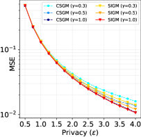
(a) $n=250$

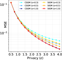
(b) $n=500$

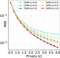
(c) $n=1000$

Figure 7: Mean Squared Error for CSGM and SIGM with $n\in\{250;500;1000\}$ and $d=500$.

Less-Trusted Server. The Distributed Discrete Gaussian (DDG) mechanism (Kairouz et al., 2021a) can leverage SecAgg to achieve DP guarantees against the server, which is a stronger setting than that of the less-trusted server. However, in practical implementation, it often requires a much higher number of bits per coordinate. The DDG mechanism relies on the discrete Gaussian distribution (Canonne et al., 2020) $\mathcal{N}_{\mathbb{Z}}(\mu,\sigma^{2})$ with $\mu,\sigma\in\mathbb{R}$ and $\sigma>0$. For any $x\in\mathbb{Z}$, $\mathbb{P}_{\mathcal{N}_{\mathbb{Z}}}(X=x)$ is proportional to $\exp(-(x-\mu)^{2}/(2\sigma^{2}))$. Using this discrete Gaussian noise, the DDG mechanism works as follows. The input parameters are: scaling factor $\gamma$; clipping threshold $c>0$; bias $\beta\geq 0$; modulus $m\in\mathbb{N}$ and noise scale $\sigma^{2}$. The shared randomness is composed of a random unitary matrix $U\in\mathbb{C}^{d\times d}$. Each client $i\in[n]$ first scales and clips the data as $x_{i}^{{}^{\prime}}=\gamma^{-1}\min\left\{1,c/\left\lVert x^{i}\right\rVert_{2}\right\}\cdot x^{i}$ then rotate $x_{i}^{{}^{\prime\prime}}$ = $Ux_{i}^{{}^{\prime}}$ and quantize $x_{i}^{{}^{\prime\prime}}$ to $M_{i}$ such that $\left\lVert M_{i}\right\rVert_{2}\leq C(\gamma,\beta,c)$. The worker finally sends to the server $\tilde{M}_{i}=M_{i}+G_{i}\mod m$, where $G_{i}\sim\mathcal{N}_{\mathbb{Z}}(0,\sigma^{2})$ using SecAgg. The server receives the results of SecAgg $\tilde{M}=\sum_{i}^{n}\tilde{M}_{i}\mod m$ and outputs $(\gamma/n)U^{*}M$ (rescale and inverse the rotation). For more details, refer to Algorithms 1 and 2 in Kairouz et al. (2021a). Note that some recent work of Chen et al. (2022) aims at improving communication efficiency of DDG by applying projections to reduce the dimension of the data transmitted. However, it still uses DDG as a subroutine so we restrict our comparison to DDG.

To compare with the utility-communication trade-off of DDG, we adapt the experiments from Kairouz et al. (2021a). On the one hand, we reproduce the figures comparing the utility of DDG with different number of bits against the standard Gaussian mechanism. On the other hand, using Elias gamma coding, we measure over $50$ runs the average number of bits needed for the aggregate Gaussian mechanism and the shifted layered quantizer to match the Gaussian mechanism. Note that only the aggregate Gaussian mechanism is compatible with SecAgg. Figures 8 and 9 below presents the mean squared error curves for different number of clients $n\in\{100;500;1000\}$ and highlights that AINQ mechanisms requires much lower number of bits to realize the Gaussian mechanism. The graphs in Figure 9 compare the number of bits per client for the shifted layered quantizer (fixed or variable length) and the aggregate Gaussian mechanism, for a privacy budget $\varepsilon\in[1,10]$.

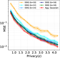
(a) $n=100$

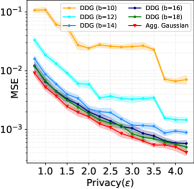
(b) $n=500$

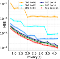
(c) $n=1000$

Figure 8: Mean Squared Error for the DDG mechanism and Aggregate Gaussian mechanism for $n\in\{100;500;1000\}$, $\delta=10^{-5}$ and $d=75$. Data samples drawn from the $\ell_{2}$ sphere with radius $c=10$.

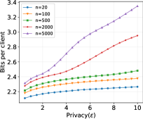
(a) Aggregate Gaussian

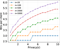
(b) Shifted Layered - Upper Bound

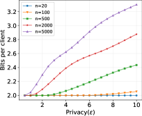
(c) Shifted Layered

Figure 9: Number of bits per clients for the Aggregation Gaussian mechanism (left), shifted layered quantizer with fixed (center) or variable (right) length and different client size $n\in\{20;100;500;2000;5000\}$.

C.2 Langevin Dynamics

C.2.1 Quantized Langevin Stochastic Dynamics

We consider the same FL framework as Vono et al. (2022) where the goal is to perform Bayesian inference on a parameter $\theta\in\mathbb{R}^{d}$ with respect to a dataset $\mathcal{D}$. The posterior distribution is assumed to admit a product-form density with respect to the $d$-dimensional Lebesgue measure in the form

$$\vspace{-0.2cm}\pi(\theta|\mathcal{D})=C_{\pi}^{-1}\prod_{i=1}^{n}e^{-U_{i}(\theta)},\qquad C_{\pi}=\int_{\mathbb{R}^{d}}\prod_{i=1}^{n}e^{-U_{i}(\theta)}\mathrm{d}\theta\vspace{-0.2cm}$$

where $U_{i}$ are clients’ potential functions. Using a sequence $(H_{k})_{k\in\mathbb{N}}$ of unbiased estimates of $\nabla U=\sum_{i=1}^{n}U_{i}$, the Langevin dynamics with stochastic gradient aims at sampling from a target distribution with density $\pi$. Starting from $\theta_{0}\in\mathbb{R}^{d}$, it is a Markov chain defined by the update rule: $\theta_{k+1}=\theta_{k}-\gamma H_{k+1}(\theta_{k})+\sqrt{2\gamma}Z_{k+1}$ where $\gamma>0$ is a discretization stepsize and $(Z_{k})_{k\in\mathbb{N}}$ is a sequence of i.i.d. standard Gaussian random variables.

In the framework of Vono et al. (2022), at iteration $k$, a subset $\mathcal{A}_{k+1}\subset[n]$ of clients is selected. Each client $i\in\mathcal{A}_{k+1}$ computes an estimate of $H_{k+1,i}$ and sends $\mathscr{C}(H_{k+1,i}-\widetilde{H}_{k+1,i})$ to the server where $\mathscr{C}$ is a compression operator and $\widetilde{H}_{k+1,i}$ is a variance reduction term. The server aggregates the clients gradients estimators, potentially compensates for the variance reduction, and updates the process. Throughout the remaining of this subsection, we consider $\mathscr{C}$ to be a shifted layered quantizer with a fixed number of bits as described at the beginning of Appendix C and returning $x+{\cal N}(0,\sigma_{b}^{2}\left\lVert x\right\rVert_{\infty}^{2}),\;\;\sigma_{b}^{2}\left\lVert x\right\rVert_{\infty}^{2}\leftarrow\mathscr{C}(x)$.

C.2.2 Experiments on Gaussian

We adapt this experiment from Vono et al. (2022). We use $n=20$ clients with data dimension $d=50$ and local potentials $U_{i}(\theta)=\sum_{j=1}^{N_{i}}\|\theta-y_{i,j}\|^{2}/2$ where $(y_{i,j})$ is a set of synthetic independent but not identically distributed observations across clients and $N_{i}=50$. The data is generated by sampling $y_{i,j}\sim{\cal N}(\mu_{i},\mathrm{I}_{d})$ with $\mu_{i}\sim{\cal N}(0,25\mathrm{I}_{d})$. We set the discretization stepsize $\gamma=5\times 10^{-4}$ and use full participation and full batch. We adapt the QLSD^⋆ algorithm from Vono et al. (2022) to leverage the error of compression in the Langevin dynamics. If the error of compression is smaller than the required error, then the server adds additional noise. Otherwise, the server adds no additional noise to the dynamics. The theoretical analysis in Vono et al. (2022) still holds with this adaptation as it still satisfies the required assumptions on the compression operator (refer to their assumption H3).

Figure 10: MSE of different methods, b refers to the number of bits, QLSD^∗ to QLSD^⋆ with unbiased quantization, QLSD^∗-MS to the algorithm with shifted layered quantization, LSD to the algorithm with no compression

Figure 10 above shows the behavior of the mean squared error (MSE) between the true parameter and the sampling based estimation. We start sampling after $4.5\times 10^{5}$ iteration to be sure the chain converge to a stationary distribution. The results were computed using $30$ independent runs of each algorithm. Observe the great performance of shifted layered quantizers schemes. Indeed, all schemes using standard unbiased quantization performs worse than all schemes with shifted layered quantizers.

Algorithm 6 QLSD^⋆ with Shifted Layered Quantizer

Input: minibatch sizes $\{n_{i}\}_{i\in[b]}$, number of iterations $K$, compression operators $\mathscr{C}$, step-size $\gamma\in(0,\bar{\gamma}]$ with $\bar{\gamma}>0$ and initial point $\theta_{0}$.

for $k=0$ to $K-1$ do

     for $i\in\mathcal{A}_{k+1}$ $\triangleright$ On active clients do

         Draw $\mathcal{S}_{k+1}^{(i)}\sim\mathrm{Uniform}\left({\wp_{N_{i},n_{i}}}\right)$.

         Set $H_{k+1}^{(i)}(\theta_{k})=(N_{i}/n_{i})\sum_{j\in\mathcal{S}_{k+1}^{(i)}}[\nabla U_{i,j}(\theta_{k})-\nabla U_{i,j}(\theta^{\star})]$.

         Compute $\textsl{g}_{i,k+1},v_{i,k+1}\leftarrow\mathscr{C}\left({H_{k+1}^{(i)}(\theta_{k})}\right)$.

         Send $\textsl{g}_{i,k+1},v_{i,k+1}$ to the central server.

     end for

     $\triangleright$ On the central server

     Compute $\textsl{g}_{k+1}=\frac{b}{|\mathcal{A}_{k+1}|}\sum_{i\in\mathcal{A}_{k+1}}\textsl{g}_{i,k+1}$.

     Draw $Z_{k+1}\sim\mathrm{N}(0_{d},\mathrm{I}_{d})$.

     Compute $\beta^{2}=\max\left(0,2\gamma-\frac{b^{2}\gamma^{2}}{|\mathcal{A}_{k+1}|^{2}}\sum_{i\in\mathcal{A}_{k+1}}v_{i,k+1}\right)$

     Compute $\theta_{k+1}=\theta_{k}-\gamma\textsl{g}_{k+1}+\beta Z_{k+1}$.

     Send $\theta_{k+1}$ to the $b$ clients.

end for

Output: samples $\{\theta_{k}\}_{k=0}^{K}$.

Appendix D Compression for Randomized Smoothing in Federated Learning

In this section, we show how the proposed quantizers with exact error distribution can be applied to obtain optimal algorithms for non-smooth distributed optimization problems (Scaman et al., 2018). In particular, we highlight the link between compression and randomized smoothing (Duchi et al., 2012). In the framework of federated learning with bi-directional compression (Philippenko and Dieuleveut, 2021), it allows us to derive fast convergence rates for non-smooth objectives. To the best of found knowledge, such rates for federated learning with client compression on non-smooth objectives are novel.

Federated Learning with double compression. Consider some optimization problems of the form

$$\min_{\theta\in\mathbb{R}^{d}}\left\{f(\theta)=\frac{1}{n}\sum_{i=1}^{n}f_{i}(\theta)\right\}$$

where $f_{i}$ are local losses and $f$ is a convex and potentially non-smooth objective function. This distributed setting includes FL problems with $\ell_{1}$ norms used as regularizers to ensure sparsity, e.g. $f(\theta)=\frac{1}{n}\|A\theta-b\|_{1}=\frac{1}{n}\sum_{i=1}^{n}|a_{i}^{\top}\theta-b_{i}|$ with $A\in\mathbb{R}^{n\times d},b\in\mathbb{R}^{n}$ but also neural networks with ReLU activation function.

In the standard setting of Federated Averaging with bi-directional compression, the model parameter $\theta_{k}$ at time step $k\in\mathbb{N}$ is updated as

$$\theta_{k+1}=\theta_{k}-\gamma\mathscr{C}_{\downarrow}\left(\frac{1}{n}\sum_{i=1}^{n}\mathscr{C}_{\uparrow}(g_{i}(\theta_{k}))\right)$$

where $\gamma>0$ is the learning rate, $\mathscr{C}_{\uparrow}$ (resp. $\mathscr{C}_{\downarrow}$) is the up-link/client compressor (resp. the down-link/server) and $g_{i}(\theta_{k})$ is a subgradient of the local loss $f_{i}$ such that $\operatorname{\mathbb{E}}[g_{i}(\theta_{k})]\in\partial f_{i}(\theta_{k})$.

Distributed Randomized Smoothing. Fast rates for non-smooth optimization problems can be attained using the smoothing approach of Duchi et al. (2012); Scaman et al. (2018). For $\sigma>0$, denote by $f_{\sigma}$ the smoothed version of $f$ defined by

$$f_{\sigma}(\theta)=\operatorname{\mathbb{E}}_{\xi}[f(\theta+\sigma\xi)],$$

where $\xi\sim\mathcal{N}(0,\mathrm{I}_{d})$ is a standard Gaussian random variable. If $f$ is $L$-Lipschitz then $f_{\sigma}$ is $(L/\sigma)$ smooth and it holds (see Lemma E.3 in Duchi et al. (2012))

$$\forall\theta\in\mathbb{R}^{d},\quad f(\theta)\leq f_{\sigma}(\theta)\leq f(\theta)+\sigma L\sqrt{d}.$$

Thus, accelerated optimization algorithms such as Distributed Randomized Smoothing (DRS) can be applied by using the smoothed version of $f$. These algorithms rely on approximating the smoothed gradient $\nabla f_{\sigma}=\frac{1}{n}\sum_{i=1}^{n}\nabla f_{i,\sigma}$ with sampled subgradients of the form $g_{i}(\theta+\sigma\xi_{j})$ with $j=1,\ldots,m$. Each local client $i=1,\ldots,n$ can sample standard Gaussian variables then compute $\hat{g}_{i}(\theta)=\frac{1}{m}\sum_{j=1}^{m}g_{i}(\theta+\sigma\xi_{j})$ and send it to the server which aggregates the subgradients. Interestingly, the sampling steps may be replaced with compressors that produce exact error distribution.

Quantizers act as randomized smoothing. The idea of sampling a random perturbation $\xi$ to evaluate the subgradients as $g_{i}(\theta+\sigma\xi)$ can be replaced by first compressing the model parameter $\theta$ with a Gaussian error distribution as ${\mathscr{E}}(\theta)=\theta+\sigma\xi$ and then evaluating the subgradients at compressed point as $g_{i}({\mathscr{E}}(\theta))$. Similarly to Philippenko and Dieuleveut (2021), let us consider the update rules where the subgradients are evaluted at perturbed point as

$$\theta_{k+1}=\theta_{k}-\frac{\gamma}{n}\sum_{i=1}^{n}\hat{g}_{i}(\hat{\theta}_{k});\quad\hat{\theta}_{k}={\mathscr{E}}(\theta_{k})=\theta_{k}+\xi_{k},$$

with a Gaussian error $\xi_{k}={\mathscr{E}}(\theta_{k})-\theta_{k}\sim\mathcal{N}(0,\sigma^{2}\mathrm{I}_{d})$. In view of approximating the sampling scheme of DRS, the local clients can perform $m$ local compressions so that $\hat{g}_{i}(\hat{\theta}_{k})=\frac{1}{m}\sum_{j=1}^{m}g_{i}(\theta_{k}+\sigma\xi_{j})$ which gives an unbiased estimate of the smoothed gradient as $\operatorname{\mathbb{E}}[\hat{g}_{i}(\hat{\theta}_{k})|\theta_{k}]=\nabla f_{i,\sigma}$. Thus, one can exactly recover the Distributed Randomized Smoothing algorithm of Scaman et al. (2018) and the optimal convergence rates of Theorem 1 therein.

References

- Abadi et al. (2016) Martin Abadi, Andy Chu, Ian Goodfellow, H. Brendan McMahan, Ilya Mironov, Kunal Talwar, and Li Zhang. Deep Learning with Differential Privacy. In Proceedings of the 2016 ACM SIGSAC Conference on Computer and Communications Security, CCS ’16, pages 308–318, Vienna, Austria, October 2016. Association for Computing Machinery. ISBN 978-1-4503-4139-4. doi: 10.1145/2976749.2978318.
- Agustsson and Theis (2020) Eirikur Agustsson and Lucas Theis. Universally quantized neural compression. In Advances in Neural Information Processing Systems 34, 2020.
- Alistarh et al. (2017) Dan Alistarh, Demjan Grubic, Jerry Li, Ryota Tomioka, and Milan Vojnovic. Qsgd: Communication-efficient sgd via gradient quantization and encoding. Advances in neural information processing systems, 30:1709–1720, 2017.
- Amiri et al. (2021) Saba Amiri, Adam Belloum, Sander Klous, and Leon Gommans. Compressive differentially private federated learning through universal vector quantization. In AAAI Workshop on Privacy-Preserving Artificial Intelligence, 2021.
- Ammah and Owusu (2019) Paul Nii Tackie Ammah and Ebenezer Owusu. Robust medical image compression based on wavelet transform and vector quantization. Informatics in medicine unlocked, 15:100183, 2019.
- Anwar et al. (2017) Sajid Anwar, Kyuyeon Hwang, and Wonyong Sung. Structured pruning of deep convolutional neural networks. ACM Journal on Emerging Technologies in Computing Systems (JETC), 13(3):1–18, 2017.
- Balle et al. (2018) Borja Balle, Gilles Barthe, and Marco Gaboardi. Privacy amplification by subsampling: Tight analyses via couplings and divergences. Advances in neural information processing systems, 31, 2018.
- Bennett et al. (2002) Charles H Bennett, Peter W Shor, John A Smolin, and Ashish V Thapliyal. Entanglement-assisted capacity of a quantum channel and the reverse shannon theorem. IEEE transactions on Information Theory, 48(10):2637–2655, 2002.
- Bonawitz et al. (2017) Keith Bonawitz, Vladimir Ivanov, Ben Kreuter, Antonio Marcedone, H Brendan McMahan, Sarvar Patel, Daniel Ramage, Aaron Segal, and Karn Seth. Practical secure aggregation for privacy-preserving machine learning. In proceedings of the 2017 ACM SIGSAC Conference on Computer and Communications Security, pages 1175–1191, 2017.
- Canonne et al. (2020) Clément L Canonne, Gautam Kamath, and Thomas Steinke. The discrete gaussian for differential privacy. Advances in Neural Information Processing Systems, 33:15676–15688, 2020.
- Chaudhuri et al. (2022) Kamalika Chaudhuri, Chuan Guo, and Mike Rabbat. Privacy-aware compression for federated data analysis. In Uncertainty in Artificial Intelligence, pages 296–306. PMLR, 2022.
- Chen et al. (2022) Wei-Ning Chen, Christopher A Choquette Choo, Peter Kairouz, and Ananda Theertha Suresh. The fundamental price of secure aggregation in differentially private federated learning. In International Conference on Machine Learning, pages 3056–3089. PMLR, 2022.
- Chen et al. (2023) Wei-Ning Chen, Dan Song, Ayfer Ozgur, and Peter Kairouz. Privacy amplification via compression: Achieving the optimal privacy-accuracy-communication trade-off in distributed mean estimation. arXiv preprint arXiv:2304.01541, 2023.
- Costello et al. (1998) Daniel J Costello, Joachim Hagenauer, Hideki Imai, and Stephen B Wicker. Applications of error-control coding. IEEE Transactions on Information Theory, 44(6):2531–2560, 1998.
- Duchi et al. (2012) John C. Duchi, Peter L. Bartlett, and Martin J. Wainwright. Randomized Smoothing for Stochastic Optimization. SIAM Journal on Optimization, 22(2):674–701, January 2012. ISSN 1052-6234. doi: 10.1137/110831659. Publisher: Society for Industrial and Applied Mathematics.
- Dwork et al. (2006) Cynthia Dwork, Frank McSherry, Kobbi Nissim, and Adam Smith. Calibrating noise to sensitivity in private data analysis. In Theory of Cryptography: Third Theory of Cryptography Conference, TCC 2006, New York, NY, USA, March 4-7, 2006. Proceedings 3, pages 265–284. Springer, 2006.
- Dwork et al. (2014) Cynthia Dwork, Aaron Roth, et al. The algorithmic foundations of differential privacy. Foundations and Trends® in Theoretical Computer Science, 9(3–4):211–407, 2014.
- Flamich et al. (2020) Gergely Flamich, Marton Havasi, and José Miguel Hernández-Lobato. Compressing images by encoding their latent representations with relative entropy coding. Advances in Neural Information Processing Systems, 33:16131–16141, 2020.
- Han et al. (2015) Song Han, Jeff Pool, John Tran, and William Dally. Learning both weights and connections for efficient neural network. Advances in neural information processing systems, 28, 2015.
- Harsha et al. (2010) P. Harsha, R. Jain, D. McAllester, and J. Radhakrishnan. The communication complexity of correlation. IEEE Trans. Inf. Theory, 56(1):438–449, Jan 2010.
- Havasi et al. (2019) Marton Havasi, Robert Peharz, and José Miguel Hernández-Lobato. Minimal random code learning: Getting bits back from compressed model parameters. In 7th International Conference on Learning Representations, ICLR 2019, 2019.
- Hegazy and Li (2022) Mahmoud Hegazy and Cheuk Ting Li. Randomized quantization with exact error distribution. In 2022 IEEE Information Theory Workshop (ITW), pages 350–355. IEEE, 2022.
- Huffman (1952) David A Huffman. A method for the construction of minimum-redundancy codes. Proceedings of the IRE, 40(9):1098–1101, 1952.
- Jacob et al. (2018) Benoit Jacob, Skirmantas Kligys, Bo Chen, Menglong Zhu, Matthew Tang, Andrew Howard, Hartwig Adam, and Dmitry Kalenichenko. Quantization and training of neural networks for efficient integer-arithmetic-only inference. In Proceedings of the IEEE conference on computer vision and pattern recognition, pages 2704–2713, 2018.
- Johnston (1988) James D Johnston. Transform coding of audio signals using perceptual noise criteria. IEEE Journal on selected areas in communications, 6(2):314–323, 1988.
- Jung et al. (2019) Sangil Jung, Changyong Son, Seohyung Lee, Jinwoo Son, Jae-Joon Han, Youngjun Kwak, Sung Ju Hwang, and Changkyu Choi. Learning to quantize deep networks by optimizing quantization intervals with task loss. In Proceedings of the IEEE/CVF Conference on Computer Vision and Pattern Recognition, pages 4350–4359, 2019.
- Kairouz et al. (2021a) Peter Kairouz, Ziyu Liu, and Thomas Steinke. The distributed discrete Gaussian mechanism for federated learning with secure aggregation. In International Conference on Machine Learning, pages 5201–5212. PMLR, 2021a.
- Kairouz et al. (2021b) Peter Kairouz, H Brendan McMahan, Brendan Avent, Aurélien Bellet, Mehdi Bennis, Arjun Nitin Bhagoji, Kallista Bonawitz, Zachary Charles, Graham Cormode, Rachel Cummings, et al. Advances and open problems in federated learning. Foundations and Trends® in Machine Learning, 14(1–2):1–210, 2021b.
- Karimireddy et al. (2020) Sai Praneeth Karimireddy, Satyen Kale, Mehryar Mohri, Sashank Reddi, Sebastian Stich, and Ananda Theertha Suresh. Scaffold: Stochastic controlled averaging for federated learning. In International Conference on Machine Learning, pages 5132–5143. PMLR, 2020.
- Konečnỳ et al. (2016) Jakub Konečnỳ, H Brendan McMahan, Felix X Yu, Peter Richtárik, Ananda Theertha Suresh, and Dave Bacon. Federated learning: Strategies for improving communication efficiency. arXiv preprint arXiv:1610.05492, 2016.
- Lang et al. (2023) Natalie Lang, Elad Sofer, Tomer Shaked, and Nir Shlezinger. Joint privacy enhancement and quantization in federated learning. IEEE Transactions on Signal Processing, 71:295–310, 2023. doi: 10.1109/TSP.2023.3244092.
- Li and El Gamal (2018) C. T. Li and A. El Gamal. Strong functional representation lemma and applications to coding theorems. IEEE Trans. Inf. Theory, 64(11):6967–6978, Nov 2018. ISSN 0018-9448. doi: 10.1109/TIT.2018.2865570.
- Li et al. (2022) Junyi Li, Jian Pei, and Heng Huang. Communication-efficient robust federated learning with noisy labels. In Proceedings of the 28th ACM SIGKDD Conference on Knowledge Discovery and Data Mining, pages 914–924, 2022.
- Li et al. (2012) Ninghui Li, Wahbeh Qardaji, and Dong Su. On sampling, anonymization, and differential privacy or, k-anonymization meets differential privacy. In Proceedings of the 7th ACM Symposium on Information, Computer and Communications Security, pages 32–33, 2012.
- Lin et al. (2018) Yujun Lin, Song Han, Huizi Mao, Yu Wang, and Bill Dally. Deep gradient compression: Reducing the communication bandwidth for distributed training. In 6th International Conference on Learning Representations, ICLR 2018, Vancouver, BC, Canada, April 30 - May 3, 2018, Conference Track Proceedings, 2018.
- Liu et al. (2017) Feng Liu, Miguel Hernandez-Cabronero, Victor Sanchez, Michael W Marcellin, and Ali Bilgin. The current role of image compression standards in medical imaging. Information, 8(4):131, 2017.
- McMahan et al. (2017) Brendan McMahan, Eider Moore, Daniel Ramage, Seth Hampson, and Blaise Aguera y Arcas. Communication-efficient learning of deep networks from decentralized data. In Artificial intelligence and statistics, pages 1273–1282. PMLR, 2017.
- Mironov (2017) Ilya Mironov. Rényi differential privacy. In 2017 IEEE 30th computer security foundations symposium (CSF), pages 263–275. IEEE, 2017.
- Noble et al. (2022) Maxence Noble, Aurélien Bellet, and Aymeric Dieuleveut. Differentially private federated learning on heterogeneous data. In International Conference on Artificial Intelligence and Statistics, pages 10110–10145. PMLR, 2022.
- Philippenko and Dieuleveut (2021) Constantin Philippenko and Aymeric Dieuleveut. Preserved central model for faster bidirectional compression in distributed settings. Advances in Neural Information Processing Systems, 34:2387–2399, 2021.
- Qu et al. (2021) Yuben Qu, Haipeng Dai, Yan Zhuang, Jiafa Chen, Chao Dong, Fan Wu, and Song Guo. Decentralized federated learning for uav networks: Architecture, challenges, and opportunities. IEEE Network, 35(6):156–162, 2021.
- Rai and Dey (2012) Brijesh Kumar Rai and Bikash Kumar Dey. On network coding for sum-networks. IEEE Transactions on Information Theory, 58(1):50–63, 2012.
- Ramamoorthy and Langberg (2013) Aditya Ramamoorthy and Michael Langberg. Communicating the sum of sources over a network. IEEE Journal on Selected Areas in Communications, 31(4):655–665, 2013.
- Rastegari et al. (2016) Mohammad Rastegari, Vicente Ordonez, Joseph Redmon, and Ali Farhadi. Xnor-net: Imagenet classification using binary convolutional neural networks. In European conference on computer vision, pages 525–542. Springer, 2016.
- Rizk and Sayed (2021) Elsa Rizk and Ali H Sayed. A graph federated architecture with privacy preserving learning. In 2021 IEEE 22nd International Workshop on Signal Processing Advances in Wireless Communications (SPAWC), pages 131–135. IEEE, 2021.
- Roberts (1962) Lawrence G. Roberts. Picture coding using pseudo-random noise. IRE Trans. Inf. Theory, 8(2):145–154, 1962. doi: 10.1109/TIT.1962.1057702.
- Sayood (2017) Khalid Sayood. Introduction to data compression. Morgan Kaufmann, 2017.
- Scaman et al. (2018) Kevin Scaman, Francis Bach, Sebastien Bubeck, Laurent Massoulié, and Yin Tat Lee. Optimal Algorithms for Non-Smooth Distributed Optimization in Networks. Advances in Neural Information Processing Systems, 31:2740–2749, 2018.
- Shah et al. (2022) Abhin Shah, Wei-Ning Chen, Johannes Balle, Peter Kairouz, and Lucas Theis. Optimal compression of locally differentially private mechanisms. In International Conference on Artificial Intelligence and Statistics, pages 7680–7723. PMLR, 2022.
- Suresh et al. (2017) Ananda Theertha Suresh, X Yu Felix, Sanjiv Kumar, and H Brendan McMahan. Distributed mean estimation with limited communication. In International conference on machine learning, pages 3329–3337. PMLR, 2017.
- Theis et al. (2022) Lucas Theis, Tim Salimans, Matthew D Hoffman, and Fabian Mentzer. Lossy compression with Gaussian diffusion. arXiv preprint arXiv:2206.08889, 2022.
- Truex et al. (2019) Stacey Truex, Nathalie Baracaldo, Ali Anwar, Thomas Steinke, Heiko Ludwig, Rui Zhang, and Yi Zhou. A Hybrid Approach to Privacy-Preserving Federated Learning. In Proceedings of the 12th ACM Workshop on Artificial Intelligence and Security, AISec’19, pages 1–11, London, United Kingdom, November 2019. Association for Computing Machinery. ISBN 978-1-4503-6833-9. doi: 10.1145/3338501.3357370.
- Vono et al. (2022) Maxime Vono, Vincent Plassier, Alain Durmus, Aymeric Dieuleveut, and Eric Moulines. Qlsd: Quantised langevin stochastic dynamics for bayesian federated learning. In International Conference on Artificial Intelligence and Statistics, pages 6459–6500. PMLR, 2022.
- Wei et al. (2020) Kang Wei, Jun Li, Ming Ding, Chuan Ma, Howard H Yang, Farhad Farokhi, Shi Jin, Tony QS Quek, and H Vincent Poor. Federated learning with differential privacy: Algorithms and performance analysis. IEEE Transactions on Information Forensics and Security, 15:3454–3469, 2020.
- Welling and Teh (2011) Max Welling and Yee W Teh. Bayesian learning via stochastic gradient langevin dynamics. In Proceedings of the 28th international conference on machine learning (ICML-11), pages 681–688, 2011.
- Wen et al. (2017) Wei Wen, Cong Xu, Feng Yan, Chunpeng Wu, Yandan Wang, Yiran Chen, and Hai Li. Terngrad: Ternary gradients to reduce communication in distributed deep learning. Advances in neural information processing systems, 30, 2017.
- Wilson (2000) David Bruce Wilson. Layered multishift coupling for use in perfect sampling algorithms (with a primer on cftp). Monte Carlo Methods, 26:141–176, 2000.
- Yang et al. (2023) Yibo Yang, Stephan Mandt, Lucas Theis, et al. An introduction to neural data compression. Foundations and Trends® in Computer Graphics and Vision, 15(2):113–200, 2023.
- Zamir and Feder (1992) Ram Zamir and Meir Feder. On universal quantization by randomized uniform/lattice quantizers. IEEE Trans. Inf. Theory, 38(2):428–436, 1992. doi: 10.1109/18.119699.
- Ziv (1985) Jacob Ziv. On universal quantization. IEEE Trans. Inf. Theory, 31(3):344–347, 1985. doi: 10.1109/TIT.1985.1057034.