Phenomenology of Lepton Masses and Mixing with Discrete Flavor Symmetries

Abstract

The observed pattern of fermion masses and mixing is an outstanding puzzle in particle physics, generally known as the flavor problem. Over the years, guided by precision neutrino oscillation data, discrete flavor symmetries have often been used to explain the neutrino mixing parameters, which look very different from the quark sector. In this review, we discuss the application of non-Abelian finite groups to the theory of neutrino masses and mixing in the light of current and future neutrino oscillation data. We start with an overview of the neutrino mixing parameters, comparing different global fit results and limits on normal and inverted neutrino mass ordering schemes. Then, we discuss a general framework for implementing discrete family symmetries to explain neutrino masses and mixing. We discuss CP violation effects, giving an update of CP predictions for trimaximal models with nonzero reactor mixing angle and models with partial $\mu-\tau$ reflection symmetry, and constraining models with neutrino mass sum rules. The connection between texture zeroes and discrete symmetries is also discussed. We summarize viable higher-order groups, which can explain the observed pattern of lepton mixing where the non-zero $\theta_{13}$ plays an important role. We also review the prospects of embedding finite discrete symmetries in the Grand Unified Theories and with extended Higgs fields. Models based on modular symmetry are also briefly discussed. A major part of the review is dedicated to the phenomenology of flavor symmetries and possible signatures in the current and future experiments at the intensity, energy, and cosmic frontiers. In this context, we discuss flavor symmetry implications for neutrinoless double beta decay, collider signals, leptogenesis, dark matter, as well as gravitational waves.

1   Introduction

Over the past few decades, we have seen spectacular progress in understanding neutrinos. The neutrino quantum oscillation phenomenon established that at least two neutrino quantum states are massive, although the masses are tiny, at the sub-electronvolt level, $m_{\nu}\lesssim{\cal{O}}(0.1)$ eV [1, 2]. A tremendous effort led to this result, as earlier experimental studies of neutrino physics faced the challenge of low event statistics for a scarce set of observables. It started around half a century ago with the pioneering Homestake experiment [3] and the so-called solar neutrino problem  [4] and culminated with the 2015 Nobel Prize in Physics for the discovery of neutrino oscillations by the Super-Kamiokande and SNO collaborations [5, 6, 7], which showed that neutrinos have mass.

The simplest neutrino mass theory is based on the three-neutrino ($3\nu$) paradigm with the assumption that flavor states ($\nu_{e},\nu_{\mu},\nu_{\tau}$) are mixed with massive states ($\nu_{1},\nu_{2},\nu_{3}$) with definite masses ($m_{1},m_{2},m_{3}$), at least two of which are non-zero. The standard parametrization of the Pontecorvo–Maki–Nakagawa–Sakata (PMNS) unitary mixing matrix reads [11, 12, 13]

$$U =U(\theta_{23})U(\theta_{13},\delta_{\rm CP})U(\theta_{12})U_{M}(\alpha_{1},\alpha_{2})$$

$$=\begin{pmatrix}1&0&0\\ 0&c_{23}&{s_{23}}\\ 0&-s_{23}&{c_{23}}\end{pmatrix}\begin{pmatrix}c_{13}&0&s_{13}e^{-i\delta_{\text{\rm CP}}}\\ 0&1&0\\ -s_{13}e^{i\delta_{\text{\rm CP}}}&0&c_{13}\end{pmatrix}\begin{pmatrix}c_{12}&s_{12}&0\\ -s_{12}&c_{12}&0\\ 0&0&1\end{pmatrix}\begin{pmatrix}e^{i\alpha_{1}}&0&0\\ 0&e^{i\alpha_{2}}&0\\ 0&0&1\end{pmatrix},$$ (1.1)

where $M$ stands for Majorana neutrinos, $c_{ij}\equiv\cos(\theta_{ij})$, $s_{ij}\equiv\sin(\theta_{ij})$, and the Euler rotation angles $\theta_{ij}$ can be taken without loss of generality from the first quadrant, $\theta_{ij}\in[0,\pi/2]$, and the Dirac CP phase $\delta_{\text{\rm CP}}$ and Majorana phases $\alpha_{1},\alpha_{2}$ are in the range $[0,2\pi]$ [14]. This choice of parameter regions is independent of matter effects [15].

In the $3\nu$ paradigm, there are two non-equivalent mass orderings: normal mass ordering (NO) with $m_{1}<m_{2}<m_{3}$ and inverted mass ordering (IO) with $m_{3}<m_{1}<m_{2}$. The neutrino masses can be further classified into normal hierarchical mass spectrum (NH) with $m_{1}\ll m_{2}<m_{3}$, inverted hierarchical mass spectrum (IH) with $m_{3}\ll m_{1}<m_{2}$ and quasi-degenerate mass spectrum (QD) with $m_{1}\simeq m_{2}\simeq m_{3}$ [14]. Within QD, quasi-degenerate NH (QDNH) mass spectrum with $m_{1}\lesssim m_{2}\lesssim m_{3}$ and quasi-degenerate IH (QDIH) mass spectrum with $m_{3}\lesssim m_{1}\lesssim m_{2}$ [16] can be distinguished. NO/IO notation is sometimes used interchangeably with NH/IH in the literature. However, NO/IO notation is more general since both NH and QDNH are NO and IH and QDIH are IO. For more discussion, see section 14.7 in the PDG review [14]. In what follows, we will use the NO/IO notation. Neutrino masses can be expressed by the smallest of the three neutrino masses ($m_{0}$) and experimentally determined mass-squared differences ($\Delta m_{21}^{2},\Delta m_{31}^{2},\Delta m_{32}^{2}$)

$$\begin{array}[]{ccc}\mbox{\text@underline{Normal mass ordering (NO)}}&\mbox{\text@underline{Inverted mass ordering (IO)}}&\\ \begin{array}[]{l}m_{1}=m_{0},\\ m_{2}=\sqrt{m_{0}^{2}+\Delta m_{21}^{2}},\\ m_{3}=\sqrt{m_{0}^{2}+\Delta m_{31}^{2}},\\ \end{array}&\begin{array}[]{l}m_{1}=\sqrt{m_{0}^{2}-\Delta m_{21}^{2}-\Delta m_{32}^{2}},\\ m_{2}=\sqrt{m_{0}^{2}-\Delta m_{32}^{2}},\\ m_{3}=m_{0},\end{array}\end{array}$$ (1.2)

where $\Delta m_{ij}^{2}\equiv m_{i}^{2}-m_{j}^{2}$. The observation of matter effects in the Sun constrains the product $\Delta m^{2}_{21}\cos{2\theta_{12}}$ to be positive [17]. By definition, we choose $\Delta m^{2}_{21}>0$ and $\theta_{12}$ in the first octant, although in presence of non-standard matter effects, a high-octant $\theta_{12}$ is possible [18].

Depending on their origin, the neutrino oscillation parameters $\theta_{12}$, $\theta_{23}$ and $\theta_{13}$ are often called solar, atmospheric and reactor angles, respectively, while $\Delta m_{21}^{2}$ and $\Delta m_{31}^{2}$ are called solar and atmospheric mass-squared differences, respectively. This naming has a historical background and is related to the neutrino source associated with measured oscillation parameters in the initial neutrino experiments.

Tab. 1.1 summarizes recent global fits for the neutrino oscillation parameters [19, 20, 21, 22, 23], which are used in the present analysis for NO/IO. The data shows a hierarchy between the mass splittings, $\Delta m_{21}^{2}\ll\Delta m_{31}^{2}\simeq\Delta m_{32}^{2}$ and preference of NO at an overall level of $\sim 2.5\sigma$ corresponding to $\Delta\chi^{2}\sim 6.4-6.5$. Lower octant atmospheric angle $\theta_{23}$ best-fit is favored for NO in NuFit 5.2 [19, 20] and Capozzi et al [23] results. These analysis include the most recent Superkamiokande (SK) data (with $\sin^{2}\theta_{23}<0.5$ preference) [24, 25]. The $\theta_{23}$ best-fit octant preference discussed above is illustrated in Fig. 1.1 together with other neutrino parameters as given in Tab.  1.1.

Parameter	Ordering	NuFit 5.2 [19, 20]		de Salas et al. (2021)  [21, 22]		Capozzi et al. (2021) [23]
		bf$\pm 1\sigma$	$3\sigma$ range	bf$\pm 1\sigma$	$3\sigma$ range	bf$\pm 1\sigma$	$3\sigma$ range
$\sin^{2}\theta_{12}/10^{-1}$	NO, IO	$3.03^{+0.12}_{-0.12}$	$2.70-3.41$	$3.18^{+0.16}_{-0.16}$	$2.71-3.69$	$3.03^{+0.13}_{-0.13}$	$2.63-3.45$
$\sin^{2}\theta_{23}/10^{-1}$	NO	$4.51^{+0.19}_{-0.16}$	$4.08-6.03$	$5.74^{+0.14}_{-0.14}$	$4.34-6.10$	$4.55^{+0.18}_{-0.15}$	$4.16-5.99$
	IO	$5.69^{+0.16}_{-0.21}$	$4.12-6.13$	$5.78^{+0.10}_{-0.17}$	$4.33-6.08$	$5.69^{+0.12}_{-0.21}$	$4.17-6.06$
$\sin^{2}\theta_{13}/10^{-2}$	NO	$2.225^{+0.056}_{-0.059}$	$2.052-2.398$	$2.200^{+0.069}_{-0.062}$	$2.000-2.405$	$2.23^{+0.07}_{-0.06}$	$2.04-2.44$
	IO	$2.223^{+0.058}_{-0.058}$	$2.048-2.416$	$2.225^{+0.064}_{-0.070}$	$2.018-2.424$	$2.23^{+0.06}_{-0.06}$	$2.03-2.45$
$\delta_{\rm CP}/\pi$	NO	$1.29^{+0.20}_{-0.14}$	$0.80-1.94$	$1.08^{+0.13}_{-0.12}$	$0.71-1.99$	$1.24^{+0.18}_{-0.13}$	$0.77-1.97$
	IO	$1.53^{+0.12}_{-0.16}$	$1.08-1.91$	$1.58^{+0.15}_{-0.16}$	$1.11-1.96$	$1.52^{+0.15}_{-0.11}$	$1.07-1.90$
$\Delta m_{21}^{2}/10^{-5}\mbox{eV}^{2}$	NO, IO	$7.41^{+0.21}_{-0.20}$	$6.82-8.03$	$7.50^{+0.22}_{-0.20}$	$6.94-8.14$	$7.36^{+0.16}_{-0.15}$	$6.93-7.93$
$\left|{\Delta m_{\rm atm}^{2}}\right|/10^{-3}\mbox{eV}^{2}$	NO	$2.507^{+0.026}_{-0.027}$	$2.427-2.590$	$2.55^{+0.02}_{-0.03}$	$2.47-2.63$	$2.485^{+0.023}_{-0.031}$	$2.401-2.565$
	IO	$2.486^{+0.028}_{-0.025}$	$2.406-2.570$	$2.45^{+0.02}_{-0.03}$	$2.37-2.53$	$2.455^{+0.030}_{-0.025}$	$2.376-2.541$
$\Delta\chi^{2}$	IO - NO	$6.4$		$6.4$		$6.5$

Table 1.1: Selection of neutrino oscillation data from NuFit 5.2 with SK atmospheric data [19, 20], de Salas et al. neutrino global fit [21, 22] and Capozzi et al. global fit [23]. Notation used by different groups is unified; namely, the atmospheric neutrino mass-squared difference parameter $\Delta m_{\rm atm}^{2}$ is defined for NuFit as $\Delta m_{31}^{2}$ for NO and $\Delta m_{32}^{2}$ for IO, for de Salas et al. as $\Delta m_{31}^{2}$ for NO/IO and for Capozzi et al. as $\Delta m_{31}^{2}-\Delta m_{21}^{2}/2$ for NO/IO. The lower octant atmospheric angle $\theta_{23}$ best-fit is favored for NO in NuFit and Capozzi et al. results, which can be related to more recent SK atmospheric data used in analyses. $\Delta\chi^{2}$ represents NO preference over IO at an overall level of $\sim 2.5\sigma$.

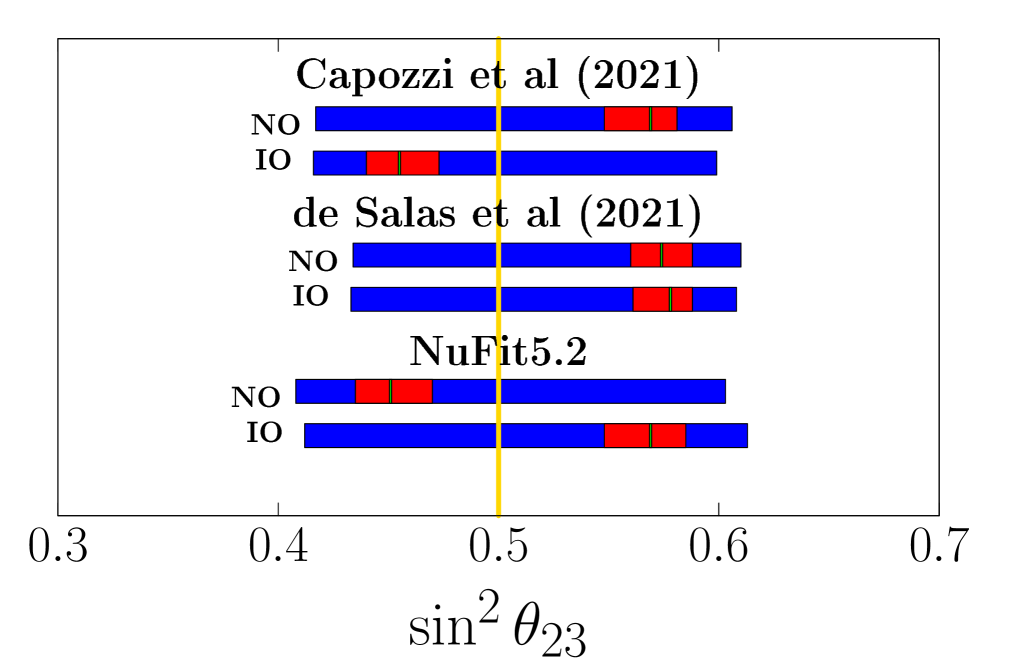
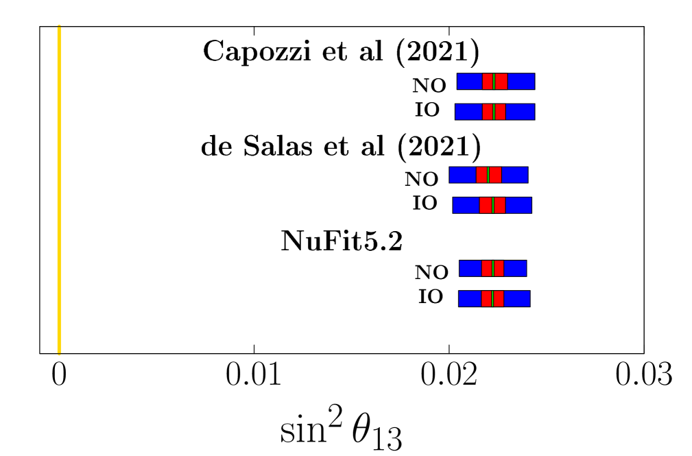
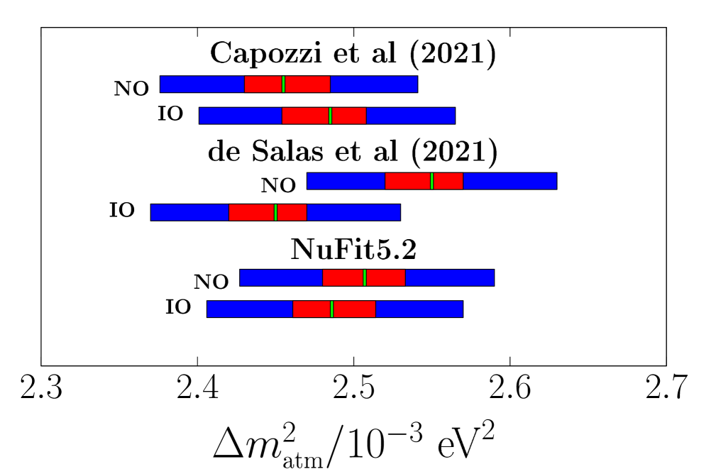
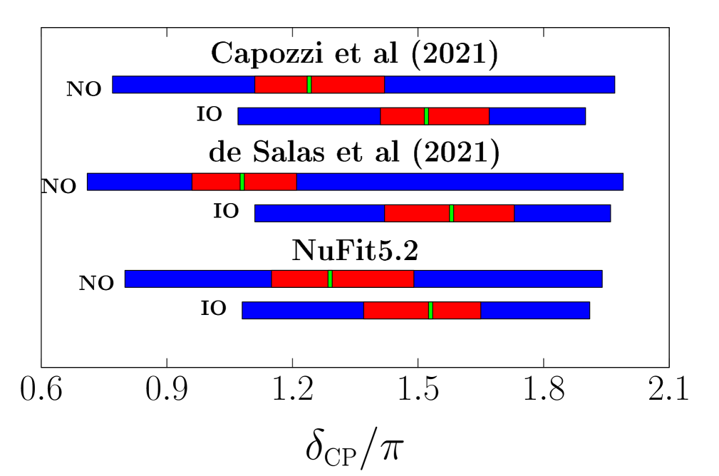
Figure 1.1: Schematics of neutrino oscillation data from Tab. 1.1. On the plots, green represents best fits, red 1$\sigma$ ranges, and blue 3$\sigma$ ranges. The golden vertical lines symbolize the historic tribimaximal (TBM) pattern values, which will be explained in Chapter 2. The plot is an update of plots presented in Refs. [26, 27].

The initial results by the T2K collaboration [28] indicated CP violation in the lepton sector, a preference for NO at the 3$\sigma$ level and also for $\theta_{23}$ in the second octant. These data are confirmed with an improved analysis [29, 30]; they continue to prefer normal mass ordering and upper octant of $\theta_{23}$ with a nearly maximal $\delta_{\rm CP}$. Also, the NO$\nu$A collaboration [31] reports on nonvanishing $\delta_{\rm CP}$ effects, though the best-fit values of CP phase differ between the two groups. Both T2K and NO$\nu$A prefer NO over IO, but T2K prefers $\delta_{\rm CP}=-90^{o}$ whereas NO$\nu$A prefers a region $\delta_{\rm CP}\sim 180^{o}$. Joint fits between NO$\nu$A +T2K and Super-K+T2K are ongoing, with the aim to obtain improved oscillation parameter constraints due to resolved degeneracies, and to understand potentially non-trivial systematic correlations [33]. The next-generation oscillation experiments, such as JUNO [34], Hyper-K [35], DUNE [36] and IceCube upgrade [37], will significantly improve the prospects of measuring $\delta_{\rm CP}$ and determining the mass ordering and the octant of $\theta_{23}$ [33].

Oscillation experiments do not put a limit on the Majorana phases $\alpha_{1}$, $\alpha_{2}$. However, predictions for the Majorana phases can be obtained using the neutrinoless double beta decay in conjunction with information on the neutrino masses [38, 39]. Also, the oscillation experiments are only sensitivity to the squared mass differences, and not to the individual masses of neutrinos. Therefore, the lightest neutrino mass $m_{0}$ is a free parameter and the other two masses are determined through Eq. (1.2). However, there are limits on the absolute neutrino mass scale from other experiments, namely, from tritium beta decay [40], neutrinoless double beta decay [41], and precision measurements of the cosmic microwave background (CMB) and large-scale structure (LSS) [42]. We discuss them now.

• A direct and model-independent laboratory constraint on the neutrino mass can be derived from the kinematics of beta decay or electron capture [40]. These experiments measure an effective electron neutrino mass

  $$m^{2}_{\beta}=\frac{\sum_{i}m^{2}_{i}|U_{ei}|^{2}}{\sum_{i}|U_{ei}|^{2}}=\sum_{i}m^{2}_{i}|U_{ei}|^{2}\,,$$ (1.3)

  assuming $U$ is unitary. This can be expressed through oscillation parameters as  [43]

  $$m^{2}_{\beta} =c_{13}^{2}c_{12}^{2}m_{1}^{2}+c_{13}^{2}s_{12}^{2}m_{2}^{2}+s_{13}^{2}m_{3}^{2}=\begin{cases}\text{NO: }&m^{2}_{0}+\Delta m^{2}_{21}c_{13}^{2}s_{12}^{2}+\Delta m^{2}_{3\ell}s_{13}^{2}\,,\\ \text{IO: }&m^{2}_{0}-\Delta m^{2}_{21}c_{13}^{2}c_{12}^{2}-\Delta m^{2}_{3\ell}c_{13}^{2}.\end{cases}$$ (1.4)

  Here $\ell=1~{}(2)$ for NO (IO) in $\Delta m^{2}_{3\ell}$. The current oscillation data impose an ultimate lower bound of $m_{\beta}>0.008~{}(0.047)$ eV for NO (IO). At present, the best direct limit on $m_{\beta}$ comes from the tritium beta decay experiment KATRIN: $m_{\beta}<0.8$ eV at 90% CL [44], with projected sensitivity down to $m_{\beta}<0.2$ eV at 90% CL [45]. The future Project 8 experiment using the Cyclotron Radiation Emission Spectroscopy (CRES) technique is expected to reach a sensitivity for $m_{\beta}$ down to 0.04 eV [46]. Some recent advances in the CRES technique were reported in Ref. [47]. Fig. 1.2 (bottom panel) summarizes present and future experimental bounds with corresponding projections to $m_{0}$ axis in NO scenario. As we can see, IO is completely within the future Project 8 sensitivity.

  

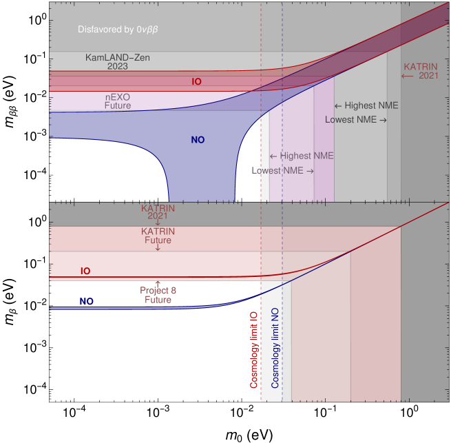
  Figure 1.2: The effective electron neutrino mass $m_{\beta}$ (Eq. (1.4)) and the effective Majorana neutrino mass $m_{\beta\beta}$ (Eq. (1.5)) plotted against the lightest neutrino mass $m_{0}$. The gray, reddish and light reddish shaded regions represent the KATRIN upper bound ($m_{\beta}<0.8\;\mbox{eV}$ at 90% CL) [44], KATRIN future bound ($m_{\beta}<0.2\;\mbox{eV}$ at 90% CL) [45] and Project 8 future bound ($m_{\beta}<0.04\;\mbox{eV}$) [46] respectively. The light gray and light magenta shaded regions represent the current upper limit range from KamLAND-Zen [48] ($36-156$ meV at 90% CL) and future sensitivity range from nEXO [49] ($4.7-20.3$ meV at 90% CL) respectively. All regions are presented with NO projections to $m_{0}$ axis. The cosmology NO/IO upper limits for $m_{0}$ correspond to the Planck data [50] (see the discussion in item (iii)).

• If neutrinos are Majorana particles, neutrinoless double beta decay ($0\nu\beta\beta$) experiments  [41] can also provide direct information on neutrino masses via the effective Majorana mass  [43]

  $$m_{\beta\beta}=\Big{|}\sum_{i}m_{i}U_{ei}^{2}\Big{|}=\Big{|}m_{1}c_{13}^{2}c_{12}^{2}e^{i2\alpha_{1}}+m_{2}c_{13}^{2}s_{12}^{2}e^{i2\alpha_{2}}+m_{3}s_{13}^{2}e^{-i2\delta_{\mathrm{CP}}}\Big{|}\\ =\begin{cases}\text{NO:}&m_{0}\,\Big{|}c_{13}^{2}c_{12}^{2}e^{i2(\alpha_{1}-\delta_{\mathrm{CP}})}+\sqrt{1+\frac{\Delta m^{2}_{21}}{m_{0}^{2}}}\,c_{13}^{2}s_{12}^{2}e^{i2(\alpha_{2}-\delta_{\mathrm{CP}})}+\sqrt{1+\frac{\Delta m^{2}_{3\ell}}{m_{0}^{2}}}\,s_{13}^{2}\Big{|}\\ \text{IO:}&m_{0}\,\Big{|}\sqrt{1-\frac{\Delta m^{2}_{3\ell}+\Delta m^{2}_{21}}{m_{0}^{2}}}\,c_{13}^{2}c_{12}^{2}e^{i2(\alpha_{1}-\delta_{\mathrm{CP}})}+\sqrt{1-\frac{\Delta m^{2}_{3\ell}}{m_{0}^{2}}}\,c_{13}^{2}s_{12}^{2}e^{i2(\alpha_{2}-\delta_{\mathrm{CP}})}+s_{13}^{2}\Big{|}.\end{cases}$$ (1.5)

  The present best upper limit on $m_{\beta\beta}$ comes from the KamLAND-Zen experiment using ${}^{136}{\rm Xe}$: $m_{\beta\beta}<0.036-0.156$ eV at 90% CL [48], where the range is due to the nuclear matrix element (NME) uncertainties. Several next-generation experiments are planned with different isotopes [51], with ultimate discovery sensitivities to $m_{\beta\beta}$ down to 0.005 eV. Based on Tab. 1.1, the update for $m_{\beta\beta}$ predictions from Eq. (1.5) as a function of the lightest neutrino mass is plotted in Fig. 1.2. The light gray shaded region shows the current upper limit range for $m_{\beta\beta}$ ($36-156$ meV at 90% CL) from KamLAND-Zen [48] (comparable limits were obtained from GERDA [52]), whereas the light magenta shaded region gives the future upper limit range for $m_{\beta\beta}$ ($4.7-20.3$ meV at 90% CL) from nEXO [49], with the shaded area in each case arising from NME uncertainties and corresponding projections to the $m_{0}$ axis in the NO scenario. Comparable future sensitivities are discussed for other experiments, such as LEGEND-1000 [53] and THEIA [54], not shown in this plot. The dark gray shaded region is disfavored by KATRIN [44]. The vertical dashed lines are the cosmological upper limits (for NO and IO) on the sum of neutrino masses ($\sum m_{i}<0.12\;\mbox{eV}$ at 95% CL) from Planck [50]; see the next item and Fig. 1.3.

• Massive neutrinos impact CMB and LSS. Thus, precision cosmological data restrict neutrino masses [55]. Here we use the most stringent limit from Planck [50]: $\sum m_{i}<0.12\;\mbox{eV}$ at 95% CL (Planck TT,TE,EE+lowE+lensing+BAO). A slightly stronger limit of $\sum m_{i}<0.09\;\mbox{eV}$ at 95% CL has been obtained in Refs. [56, 57], while Ref. [58] has argued in favor of a weaker limit of $\sum m_{i}<0.26\;\mbox{eV}$. Sum of light neutrino masses $\sum m_{i}$ is plotted in Fig. 1.3 against the lightest neutrino mass $m_{0}$ (left), effective electron neutrino mass $m_{\beta}$ (middle) and effective Majorana mass $m_{\beta\beta}$ (right) with the NuFit $3\sigma$ oscillation parameters from Tab. 1.1 for both NO and IO scenarios. The horizontal gray-shaded region represents the current Planck upper limit [50]. Future cosmology sensitivity forecast is represented by the brown-green shaded area, with an uncertainty of the order of 15 meV [59] (see also  [60]). The dashed lines represent the lowest allowed values of $\sum m_{i}=58$ meV (NO) and 97 meV (IO) by current oscillation data.

  

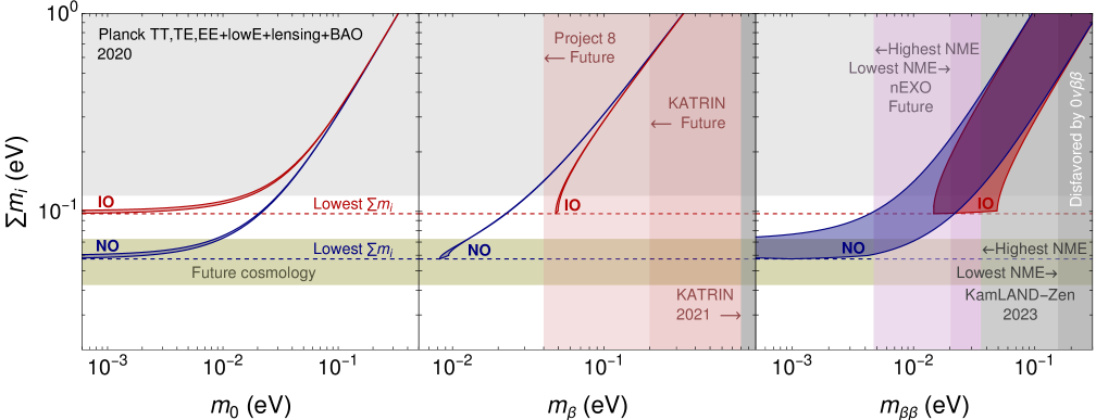
  Figure 1.3: Sum of light neutrino masses $\sum m_{i}$ plotted against the lightest neutrino mass $m_{0}$ (left), effective electron neutrino mass $m_{\beta}$ (middle) and effective Majorana mass $m_{\beta\beta}$ (right) with the NuFit $3\sigma$ oscillation parameters from Tab. 1.1. The horizontal gray-shaded region represents the current Planck upper limit [50]. Future cosmology sensitivity forecast is represented by a brown-green shaded area, with an uncertainty of the order of 15 meV [59] (see also Ref. [60]). The lowest allowed values of $\sum m_{i}$ for NO and IO from NuFit data are also shown by the dashed lines. Other current and future exclusion regions shown here are described in Fig. 1.2. The plot is an updated variation of the plot presented in Ref. [57].

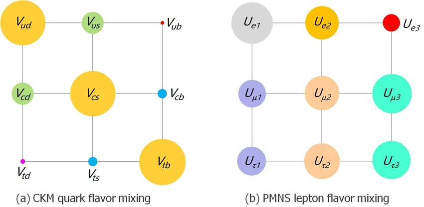
Figure 1.4: Flavor puzzle. Sizes of circles represent magnitudes of mixing among quarks (on the left) and neutrinos (on the right). Figure taken from the arXiv version of Ref. [61].

Understanding the pattern of neutrino mixing is crucial because it is part of the long-standing flavor puzzle. As seen with the naked eye in Fig. 1.4, the mixing patterns for quarks and neutrinos are intrinsically very different. The neutrino case is more "democratic" except for the $U_{e3}$ parameter, which is proportional to the small $s_{13}$ in Eq. (1.1). In fact, before the non-zero $\theta_{13}$ discovery by Daya Bay [62] and RENO [63] in 2012, the reactor mixing angle $\theta_{13}$ was thought to be vanishingly small. Guided by the $\theta_{13}\sim 0^{\circ}$ assumption and to be consistent with the observed solar and atmospheric mixing angles, several flavor mixing schemes were postulated. By substituting $\theta_{13}=0^{\circ}$ and $\theta_{23}=45^{\circ}$ in the general lepton mixing matrix given in Eq. (1.1), up to the phase matrix $U_{M}$, most of the popular mixing schemes such as bi-maximal (BM) [64, 65, 66, 67], tribimaximal (TBM) [68, 69], hexagonal (HG) [70], and golden ratio (GR) [71, 72, 73, 74, 75, 76] mixing schemes can be altogether written as

$$U_{0}=\left(\begin{array}[]{ccc}c_{12}&s_{12}&0\\ -\frac{s_{12}}{\sqrt{2}}&\frac{c_{12}}{\sqrt{2}}&-\frac{1}{\sqrt{2}}\\ -\frac{s_{12}}{\sqrt{2}}&\frac{c_{12}}{\sqrt{2}}&\frac{1}{\sqrt{2}}\end{array}\right).$$ (1.9)

Substituting $s_{12}=1/\sqrt{2},~{}1/\sqrt{3},~{}1/2$, and $\tan\theta_{12}=1/\varphi$ (with $\varphi=(1+\sqrt{5})/2$ being the golden ratio), one can explicitly obtain the fixed mixing schemes BM, TBM, HG and GR respectively. In each case the Dirac CP phase $\delta_{\rm CP}$ is undefined as $\theta_{13}=0$ and can be easily extended to include the non-vanishing Majorana phases defined in Eq. (1.1) via the definition $U_{0}\rightarrow U_{0}U_{M}$. Using the diagonalization relation

$$m_{\nu}=U_{0}^{\star}{\rm diag}(m_{1},m_{2},m_{3})U_{0}^{\dagger},$$ (1.10)

such a mixing matrix can easily diagonalize a $\mu-\tau$ symmetric (transformations $\nu_{e}\rightarrow\nu_{e}$, $\nu_{\mu}\rightarrow\nu_{\tau}$, $\nu_{\tau}\rightarrow\nu_{\mu}$ under which the neutrino mass term remains unchanged) neutrino mass matrix of the form [61]

$$m_{\nu}=\left(\begin{array}[]{ccc}A&B&B\\ B&C&D\\ B&D&C\end{array}\right),$$ (1.14)

where the elements $A,B,C$ and $D$ are in general complex. With $A+B=C+D$ this matrix yields the TBM mixing pattern

$$U_{\rm TBM}=\left(\begin{array}[]{ccc}\sqrt{\frac{2}{3}}&\frac{1}{\sqrt{3}}&0\\ -\frac{1}{\sqrt{6}}&\frac{1}{\sqrt{3}}&-\frac{1}{\sqrt{2}}\\ -\frac{1}{\sqrt{6}}&\frac{1}{\sqrt{3}}&\frac{1}{\sqrt{2}}\end{array}\right)\,.$$ (1.18)

Such first-order approximations of the neutrino oscillation data motivated theorists to find other symmetry-based aesthetic frameworks which can lead towards these fixed mixing matrices.

In this regard, non-Abelian discrete groups turned out to be popular as appropriate flavor symmetries for the lepton sector. Discrete groups have always played a key role in physics starting from crystallographic groups in solid-state physics, to discrete symmetries such as $C$, $P$, and $T$, which have shaped our understanding of nature. In neutrino physics, for a long time, various discrete groups such as $S_{3}$, $A_{4}$, $S_{4}$, $A_{5}$, $T^{\prime}$, $\Delta(27)$, $D_{n}$, $T_{7}$, $\Delta(6n^{2})$ [77, 78, 26] etc. have been extensively used to explain fermion mixing. Among the various discrete groups used for this purpose, $A_{4}$ emerged as the most widely adopted choice initially proposed as an underlying family symmetry for quark sector [79, 80]. Interestingly, in the last decade, thanks to the reactor neutrino experiments Double Chooz [81], Daya Bay [62], and RENO [63] (also T2K [82], MINOS [83], and others [84]), the reactor neutrino mixing angle is conclusively measured to be ‘large’ (see Tab. 1.1). In addition to this, as mentioned earlier, a non-zero value of the Dirac CP phase $\delta_{\rm CP}$ is favored by the oscillation experiments. Such an observation has ruled out the possibility of simple neutrino mixing schemes like in Eq. (1.9). Therefore, it is consequential to find modifications, corrections or the successors of the above mixing schemes which are still viable; this will be discussed in the next Chapter. Models based on non-Abelian discrete flavor symmetries often yield interesting predictions and correlations among the neutrino masses, mixing angles and CP phases.  Involvement of such studies may have broader applications in various aspects of cosmology (matter-antimatter asymmetry of the Universe, DM, gravitational waves), collider physics and other aspects of particle physics, which will be discussed in subsequent Chapters.

Moreover, the light neutrino sector and masses connected with three families of neutrinos and charged leptons can be a reflection of a more general theory where weakly interacting (sterile) neutrinos exist with much higher masses (GeV, TeV, or higher up to the GUT scale). A related problem is the symmetry of the full neutrino mass matrix, including the sterile sector. In this framework, the known neutrino mass and flavor states can be denoted by ${|{\nu^{(m)}_{i}}\rangle}$ and ${|{\nu^{(f)}_{\alpha}}\rangle}$, respectively, where $i=1,2,3$ and $\alpha=e,\mu,\tau$. Any extra, beyond SM (BSM) sterile mass and flavor states (typically much heavier than the active ones) can be denoted by $|{\widetilde{\nu}^{(m)}_{j}}\rangle$ and $|{\widetilde{\nu}^{(f)}_{\beta}}\rangle$, respectively for $j,\beta=1,\ldots,n_{R}$. In this general scenario mixing between an extended set of neutrino mass states $\{|{\nu^{(m)}_{i}}\rangle,|{\widetilde{\nu}^{(m)}_{j}}\rangle\}$ with flavor states $\{|{\nu^{(f)}_{\alpha}}\rangle,|{\widetilde{\nu}^{(f)}_{\beta}}\rangle\}$ is described by

$$\begin{pmatrix}{|{\nu^{(f)}_{\alpha}}\rangle}\\ |{\widetilde{\nu}^{(f)}_{\beta}}\rangle\end{pmatrix} =\begin{pmatrix}{{U}}&V_{lh}\\ V_{hl}&V_{hh}\end{pmatrix}\begin{pmatrix}{|{\nu^{(m)}_{i}}\rangle}\\ |{\widetilde{\nu}^{(m)}_{j}}\rangle\end{pmatrix}\equiv{\cal U}\begin{pmatrix}{{|{\nu^{(m)}_{i}}\rangle}}\\ |{\widetilde{\nu}^{(m)}_{j}}\rangle\end{pmatrix}\;.$$ (1.19)

The SM flavor states $|{\nu^{(f)}_{\alpha}}\rangle$ are then given by

$$|{\nu^{(f)}_{\alpha}}\rangle=\sum_{i=1}^{3}\underbrace{\left(U\right)_{\alpha i}{|{\nu^{(m)}_{i}}\rangle}}_{\rm SM\;part}+\sum_{j=1}^{n_{R}}\underbrace{{\left(V_{lh}\right)}_{\alpha j}|{\widetilde{\nu}^{(m)}_{j}}\rangle}_{\rm BSM\;part}\;.$$ (1.20)

The mixing matrix $\cal{U}$ in (1.19) diagonalizes a general neutrino mass matrix

$$M_{\nu}=\left(\begin{array}[]{cc}M_{L}&M_{D}\\ M_{D}^{T}&M_{R}\end{array}\right),$$ (1.21)

using a congruence transformation

$${\cal U}^{T}M_{\nu}{\cal U}\simeq{\rm diag}(m_{i},M_{j}).$$ (1.22)

The structure and symmetry of the heavy neutrino sector $M_{R}$ in Eq. (1.21), altogether with $M_{D}$ variants, influence the masses and mixing of the light sector, beginning with the seesaw type of models  [85]. The extended unitary mixing matrix ${\cal U}$ in (1.19), with nonzero submatrices $V$, makes $U$ nonunitary. In fact, oscillation experiments do not exclude such cases, giving the following ranges of elements [86] (present analysis and future projections):

$$\left\lvert U^{\rm Current}\right\rvert^{2}_{3\sigma} =\left(\begin{array}[]{c c c}\left[0.606,0.742\right]&\left[0.265,0.337\right]&\left[0.020,0.024\right]\\ \left[0.051,0.270\right]&\left[0.198,0.484\right]&\left[0.392,0.620\right]\\ \left[0.028,0.469\right]&\left[0.098,0.685\right]&\left[0.140,0.929\right]\end{array}\right),$$ (1.26)

$$\left\lvert U^{\rm Future}\right\rvert^{2}_{3\sigma} =\left(\begin{array}[]{c c c}\left[0.653,0.699\right]&\left[0.291,0.311\right]&\left[0.020,0.024\right]\\ \left[0.074,0.108\right]&\left[0.355,0.454\right]&\left[0.447,0.561\right]\\ \left[0.129,0.359\right]&\left[0.212,0.423\right]&\left[0.349,0.595\right]\end{array}\right).$$ (1.30)

As can be seen from these numbers, the current (and future) precision on the nonunitarity of the neutrino mixing matrix is still far away from the ultra-high precision achieved in the quark sector [87]. The interval matrices (1.26) and (1.30) include nonunitary cases. This information can be used to derive bounds between known three neutrino flavors and additional neutrino states [88, 89]. Neutrino mixing constructions based on discrete flavor symmetries discussed in the next chapters are based on unitary $3\times 3$ mixing matrices and variants of non-unitary distortions.

The number of model-building options available with discrete flavor symmetries is vast, and many have already been thoroughly reviewed in the literature. In Ref. [77], the authors have presented a pedagogical review of various non-Abelian discrete groups, including their characters, conjugacy classes, representation, and tensor products, which are essential for particle physics phenomenology. In Ref. [78], the authors discussed the application of non-Abelian finite groups to the theory of neutrino masses and mixing with $\theta_{13}\sim 0$ to reproduce fixed mixing schemes like TBM and BM, based on finite groups like $A_{4},S_{4}$, etc. After measurement of the reactor mixing angle, in Ref. [26], the authors reviewed various discrete family symmetries and their (in)direct model-building approaches. They also discussed combining grand unified theories with discrete family symmetry to describe all quark and lepton masses and mixing. In Ref. [90], the author reviewed the scenarios for flavor symmetry combined with generalized CP symmetry to understand the observed pattern of neutrino mixing and the related predictions for neutrino mixing angles and leptonic Dirac CP violation. Finally, along with conventional flavor symmetric approaches, in Ref. [91], the authors also reviewed the modular invariance approach to the lepton sector. Many other excellent reviews also partially cover issues discussed here [92, 93, 94, 95, 96, 97, 98]; see also the Snowmass contributions [99, 100, 101, 102]. Apart from the update to the mentioned reviews, our main focus in this review is a discussion on the phenomenology and testability of discrete flavor symmetries at the energy, intensity, and cosmic frontier experiments.

The rest of the review is organized as follows. In Chapter 2, we present a general framework for understanding neutrino masses and mixing with non-Abelain discrete flavor symmetries, discuss the compatibility of a few surviving mixing schemes with present neutrino oscillation data, and elaborate on explicit flavor models. We also mention various neutrino generation mechanisms and possible consequences once we augment them with discrete flavor symmetries. Then, we discuss the implications of combining flavor symmetries with CP, higher order discrete groups, Grand Unified Theories, extended Higgs sector, and finally, allude to the recently revived modular invariance approach to address the flavor problem. In Chapter 3, we discuss the impact of discrete flavor symmetries in intensity frontiers such as neutrino oscillation experiments, neutrinoless double beta decay, lepton flavor and universality violation. Then in Chapter 4, with some specific examples, we elaborate on the role of flavor symmetry at colliders, which includes a discussion on prospects of right-handed neutrino detection at colliders, lepton flavor violation and constraints on the $h\to\gamma\gamma$ decay width. In Chapter 5, we elaborate on the consequences of flavor symmetry at cosmic frontier, including studies on DM, leptogenesis and gravitational waves. Finally, in Chapter 6, we summarize and conclude.

2   Flavor Symmetry and Lepton Masses and Mixing: Theory

From Eq. (1.1) we find that the neutrino mixing matrix is expressed in terms of mixing angles and CP violating phases, and we are yet to understand the experimentally observed mixing pattern [20]. The masses and mixing of the leptons (as well as of the quarks) are obtained from the Yukawa couplings related to the families. Therefore, it is natural to ask whether any fundamental principle governs such a mixing pattern.

2.1   General Framework

The primary approaches which try to address the issue of the neutrino mixing pattern include (i) random analysis without imposing prior theories or symmetries on the mass and mixing matrices [103, 104, 105]; (ii) more specific studies with imposed mass or mixing textures for which models with underlying symmetries can be sought [106, 107, 108, 109, 110], and finally, (iii) theoretical studies where some explicit symmetries at the Yukawa Lagrangian level are assumed and corresponding extended particle sector is defined. In the anarchy hypothesis (i), the leptonic mixing matrix manifests as a random draw from an unbiased distribution of unitary $3\times 3$ matrices and does not point towards any principle or its origin. This hypothesis does not make any correlation between the neutrino masses and mixing parameters. However, it predicts probability distribution for the parameters which parameterize the mixing matrix. Though random matrices cannot solve fundamental problems in neutrino physics, they generate intriguing hints on the nature of neutrino mass matrices. For instance, in Ref. [111], preference has been observed towards random models of neutrino masses with sterile neutrinos. In the intermediate approach (ii), some texture zeros of neutrino mass matrices can be eliminated. For instance, in Ref. [109] 570 (298) inequivalent classes of texture zeros in the Dirac (Majorana) case were found. For both cases, about 75% of the classes are compatible with the data. In the case of maximal texture zeros in the neutrino and charged lepton mass matrices, there are only about 30 classes of texture zeros for each of the four categories defined by Dirac/Majorana nature and normal/inverted ordering of the neutrino mass spectrum. Strict texture neutrino mass matrices can also be discussed in phenomenological studies. For more, see section 2.3.

In what follows, we will discuss the symmetry-based approach (iii) to explain the non-trivial mixing in the lepton sector known as family symmetry or horizontal symmetry. Such fundamental symmetry in the lepton sector can easily explain the origin of neutrino mixing, which is considerably different from quark mixing. Incidentally, both Abelian and non-Abelian family symmetries have the potential to shed light on the Yukawa couplings. The Abelian symmetries (such as Froggatt-Nielsen symmetry [112]) only point towards a hierarchical structure of the Yukawa couplings, whereas non-Abelian symmetries are more equipped to explain the non-hierarchical structures of the observed lepton mixing as observed by the oscillation experiments.

If we consider a family symmetry $G_{f}$, the three generations of leptons and quarks can be assigned to irreducible representations or multiplets, hence unifying the flavor of the generations. If $G_{f}$ contains a triplet representation ($3$), all three fermion families can follow the same transformation properties. For example, let us consider that non-zero neutrino mass is generated through the Weinberg operator $HL^{T}cLH$ where the lepton and Higgs doublets transform as a triplet ($\mathbf{\bar{3}}$) and singlet under a family symmetry, say, $SU(3)$. To construct $SU(3)$ invariant operator, an additional scalar field $\Phi$ (also known as flavon ) is introduced, and the effective operator takes the form $HL^{T}\Phi^{T}\Phi LH$. A suitable vacuum alignment ($\langle\Phi\rangle\propto(u_{1},u_{2},u_{3})^{T}$) for the flavon is inserted in such a way that the obtained mass matrix is capable of appropriate mixing pattern. As a result, $G_{f}$ is spontaneously broken once flavons acquire non-zero vacuum expectation values (VEV). Continuous family symmetry such as $U(3)$, $O(3)$ (and their subgroups $SU(3)$ and $SO(3)$) can in principle be used for this purpose to understand the neutrino mixing. However, the non-Abelian discrete flavor symmetric approach is much more convenient as in such a framework, obtaining the desired vacuum alignment (which produces correct mixing) of the flavon can be obtained easily [113, 114]. At this point, it is worth mentioning that these non-Abelian discrete symmetries can also originate from a continuous symmetry [115, 116, 117, 118, 119, 120, 121, 122, 123]. For example widely used discrete groups such as $A_{4},S_{4},A_{5},\Delta(27),T_{7}$ can originate from the continuous group $SU(3)$ [26]. In another example [120], the authors showed that continuous $SO(3)$ can also give rise to $A_{4}$, further broken into smaller $Z_{3}$ and $Z_{2}$ symmetries. A few years back, it was proposed that various non-Abelian discrete symmetries can also originate from superstring theory through compactification of extra dimensions and known as the modular invariance approach [114, 94, 124].

In this report, we concentrate on all these aspects of discrete family symmetries discussed above and their implications for understanding lepton mixing and its extensions. The model building with flavor symmetries is not trivial since the underlying flavor symmetry group $G_{f}$ must be broken. Usually, this symmetry $G_{f}$ is considered to exist at some large scale (sometimes with proximity to GUT scale [78]) and to be broken at lower energies with residual symmetries of the charged lepton and neutrino sectors, represented by the subgroups $G_{e}$ and $G_{\nu}$, respectively. Therefore, to obtain definite predictions and correlations of the mixing, the choice of the non-Abelian discrete group $G_{f}$ and its breaking pattern to yield remnant subgroups $G_{e}$ and $G_{\nu}$ shapes the model building significantly. Without any residual symmetry, the flavor $G_{f}$ loses its predictivity markedly. For a detailed discussion on the choice of various discrete symmetries and their generic predictions, see Refs. [26, 90, 95].

Group	Order	Irreducible Representations	Generators
$A_{4}$	12	$1,1^{\prime},1^{\prime\prime},3$	$S,T$
$S_{4}$	24	$1,1^{\prime},2,3,3^{\prime}$	$S,T(U)$
$T^{\prime}$	24	$1,1^{\prime},1^{\prime\prime},2,2^{\prime},2^{\prime\prime},3$	$S,T(R)$
$\Delta(27)$	27	$1_{r,s}(r,s=0,1,2),3_{01,02}$	$C,D$
$A_{5}$	60	$1,3,3^{\prime},4,5$	$\tilde{S}$, $\tilde{T}$

Table 2.1: Basic characteristics of a few small groups with triplet irreducible representations. For details, see Ref. [77]. For instance, a possible representation for generators of the $S_{4}$ group is defined in the text, see Eqs. (2.1) and (2.11).

In Tab. 2.1, we mention the basic details such as order or number of elements (first and second columns), irreducible representations (third column) and generators (fourth column) of small groups (which contain at least one triplet) such as $A_{4},S_{4},T^{\prime}$ $\Delta(27)$ and $A_{5}$. A pedagogical review, including catalogues of the generators and multiplication rules of these widely used non-Abelian discrete groups, can be found in Ref. [77].

Now, for model building purposes, there exist various approaches based on the breaking pattern of $G_{f}$ into its residual symmetries, also known as direct, semi-direct and indirect approaches  [26, 95]. After breaking of $G_{f}$, different residual symmetries exist for charged lepton (typically $G_{e}=Z_{3}$) and neutrino sector (typically $G_{\nu}=Z_{2}\times Z_{2}$, also known as the Kline symmetry). It is known as the direct approach. In a semi-direct approach, one of the generators of the residual symmetry is assumed to be broken. On the contrary, in the indirect approach, no residual symmetry of flavor groups remains intact, and the flavons acquire special vacuum alignments whose alignment is guided by the flavor symmetry. Usually, different flavons take part in the charged lepton and neutrino sectors. To show how the family symmetry shapes the flavor model building, let us consider $G_{f}=S_{4}$ as a guiding symmetry. Geometrically, this group can be seen as the symmetry group of a rigid cube, a group of permutation four objects. Therefore, the order of the group is $4!=24$ and the elements can be conveniently generated by the generators $S,T$ and $U$ satisfying the relation

$$S^{2}=T^{3}=U^{2}=1~{}~{}{\rm and}~{}~{}ST^{3}=(SU)^{2}=(TU)^{2}=1.$$ (2.1)

In their irreducible triplet representations, these three generators can be written as [77, 78]

$$S=\frac{1}{3}\left(\begin{array}[]{ccc}-1&2&2\\ 2&-1&2\\ 2&2&-1\end{array}\right);T=\left(\begin{array}[]{ccc}1&0&0\\ 0&\omega^{2}&0\\ 0&0&\omega\end{array}\right)~{}~{}{\rm and}~{}~{}U=\mp\left(\begin{array}[]{ccc}1&0&0\\ 0&0&1\\ 0&1&0\end{array}\right).$$ (2.11)

where $\omega=e^{2i\pi/3}$. These generators can also be expressed as 3-dimensional irreducible (faithful) real representation matrices

$$S=\left(\begin{array}[]{ccc}-1&0&0\\ 0&1&0\\ 0&0&-1\end{array}\right);T=\frac{1}{2}\left(\begin{array}[]{ccc}1&\sqrt{2}&1\\ \sqrt{2}&0&-\sqrt{2}\\ -1&\sqrt{2}&-1\end{array}\right)~{}~{}{\rm and}~{}~{}U=\mp\left(\begin{array}[]{ccc}1&0&0\\ 0&1&0\\ 0&0&-1\end{array}\right).$$ (2.21)

In the direct approach the charged lepton mass matrix ($M_{\ell}$) respects the generator $T$ whereas the neutrino mass matrix ($M_{\nu}$) respects the generators $S,U$ satisfying the conditions

$$T^{\dagger}M_{\ell}^{\dagger}M_{\ell}T=M_{\ell}^{\dagger}M_{\ell},~{}S^{T}M_{\nu}S=M_{\nu}~{}{\rm and}~{}U^{T}M_{\nu}U=M_{\nu},$$ (2.22)

which leads to [95]

$$[T,M_{\ell}^{\dagger}M_{\ell}]=[S,M_{\nu}]=[U,M_{\nu}]=0.$$ (2.23)

The non-diagonal matrices $S,U$ can be diagonalized by the TBM mixing matrix given in Eq. (1.18). Therefore, the TBM mixing scheme can be elegantly derived from the direct approach of the $S_{4}$ group. For generic features of semi-direct and indirect approaches to the flavor model building, we refer the readers to [26, 97, 95]. The TBM mixing pattern explained here can be generated using various discrete groups. For detailed models and groups see $A_{4}$ [125, 126, 113, 114], $S_{4}$ [127, 128], $\Delta(27)$ [129], $T^{\prime}$ [130]. In addition, explicit models with discrete flavor symmetry for BM [131, 132, 133, 134], GR [73, 135, 76], HG [136] mixing can easily be constructed.

2.2   Flavor Symmetry, Nonzero $\theta_{13}$ and Nonzero $\delta_{\rm CP}$

After precise measurement of the non-zero value of the reactor mixing angle $\theta_{13}$ [81, 62, 63, 83, 82] the era of fixed patterns (such as BM, TBM, GR, HG mixing) of the lepton mixing matrix is over. Also, as mentioned earlier, long baseline neutrino oscillation experiments such as T2K [137] and NO$\nu$A [138] both hint at CP violation in the lepton sector. Therefore, each of the fixed patterns needs some modification to be consistent with the global fit of the neutrino oscillation data [19, 20, 21, 22, 23]. There are two distinct ways of generating a mixing pattern that appropriately deviates from fixed mixing schemes such as BM, TBM, GR, and HG. The first approach is based on symmetry assertion, which demands considering larger symmetry groups that contain a larger residual symmetry group compared to the fixed mixing schemes such us TBM [94, 139, 140, 141, 142, 143]. On the other hand, in the second approach, the setups for the BM, TBM, GR, and HG mixing schemes are supplemented by an additional ingredient which breaks these structures in a well-defined and controlled way [144]. This can be achieved in various ways. An apparent source for such corrections can be introduced through the charged lepton sector [145, 146, 147, 148, 149]. Thus, in models where in the neutrino sector the mass matrix solely reproduces the mixing scheme, a non-diagonal charged lepton sector will contribute to the PMNS matrix $U=U_{\ell}^{\dagger}U_{\nu}$ where $U_{\ell}$ and $U_{\nu}$ respectively are the diagonalizing matrices of the charged lepton and neutrino mass matries. In addition, one can also consider small perturbations around the BM/TBM/GR/HG vacuum-alignment conditions [150, 151, 152, 153], which can originate from higher dimensional operators in the flavon potential yielding desired deviation. The minimal flavon field content can also be extended to incorporate additional contributions to the neutrino mass matrix to achieve correct deviation from fixed mixing schemes [154, 155, 156, 157, 158, 159]. To summarize, the fixed mixing schemes can still be regarded as a first approximation, necessitating specific corrections to include non-zero $\theta_{13}$ and $\delta_{\rm CP}$. For example, even if the TBM mixing is obsolete, two successors are still compatible with data. These are called TM₁ and TM₂ mixing and are given by

$$|U_{{\rm TM}_{1}}|=\left(\begin{array}[]{ccc}\frac{2}{\sqrt{6}}&*&*\\ \frac{1}{\sqrt{6}}&*&*\\ \frac{1}{\sqrt{6}}&*&*\end{array}\right)~{}{\rm and}~{}|U_{{\rm TM}_{2}}|=\left(\begin{array}[]{ccc}*&\frac{1}{\sqrt{3}}&*\\ &\frac{1}{\sqrt{3}}&*\\ &\frac{1}{\sqrt{3}}&*\end{array}\right),$$ (2.30)

respectively. Clearly, Eq. (2.30) shows that TM₁ and TM₂ mixings preserve the first and the second column of the TBM mixing matrix given in Eq. (1.18). Here, the reactor mixing angle becomes a free parameter, and the solar mixing angle can stick close to its TBM prediction.

To illustrate this, let us again consider the discrete flavor symmetry $G_{f}=S_{4}$. In contrast to the breaking pattern mentioned in Eqs. (2.22), (2.23), $S_{4}$ is considered to be broken spontaneously into $Z_{3}=\{1,T,T^{2}\}$ (for the charged lepton sector) and $Z_{2}=\{1,SU\}$ (for the neutrino sector) such that it satisfies

$$[T,M_{\ell}^{\dagger}M_{\ell}]=[SU,M_{\nu}]=0.$$ (2.31)

Following the above prescription, the matrix that diagonalizes $SU$ (see Eq. (2.11)) can be written as $U_{\rm TBM}U_{23}(\theta,\gamma)$ where the ‘23’ rotation matrix is given by ($c_{\theta}=\cos\theta$, $s_{\theta}=\sin\theta$ and $\gamma$ is the associated phase factor)

$$U_{{23}}=\left(\begin{array}[]{ccc}1&0&0\\ 0&c_{\theta}&s_{\theta}e^{-i\gamma}\\ 0&-s_{\theta}e^{i\gamma}&c_{\theta}\end{array}\right).$$ (2.35)

The obtained effective mixing matrix is called $U_{{\rm TM}_{1}}$ and can be written as

$$U_{{\rm TM}_{1}}=\left(\begin{array}[]{ccc}\frac{2}{\sqrt{6}}&\frac{c_{\theta}}{\sqrt{3}}&\frac{s_{\theta}}{\sqrt{3}}e^{-i\gamma}\\ -\frac{1}{\sqrt{6}}&\frac{c_{\theta}}{\sqrt{3}}-\frac{s_{\theta}}{\sqrt{2}}e^{i\gamma}&-\frac{s_{\theta}}{\sqrt{3}}e^{-i\gamma}-\frac{c_{\theta}}{\sqrt{2}}\\ -\frac{1}{\sqrt{6}}&\frac{c_{\theta}}{\sqrt{3}}-\frac{s_{\theta}}{\sqrt{2}}e^{i\gamma}&-\frac{s_{\theta}}{\sqrt{3}}e^{-i\gamma}+\frac{c_{\theta}}{\sqrt{2}}\end{array}\right),$$ (2.39)

The above matrix has the TM₁ mixing structure mentioned in Eq. (2.30). This is also an example of the method of a semi-direct approach to the flavor model building. Similarly, the generic structure for the structure for TM₂ mixing matrix can be written as

$$U_{{\rm TM}_{2}}=\left(\begin{array}[]{ccc}\frac{2c_{\theta}}{\sqrt{6}}&\frac{1}{\sqrt{3}}&\frac{2s_{\theta}}{\sqrt{6}}e^{-i\gamma}\\ -\frac{c_{\theta}}{\sqrt{6}}+\frac{s_{\theta}}{\sqrt{2}}e^{i\gamma}&\frac{1}{\sqrt{3}}&-\frac{s_{\theta}}{\sqrt{3}}e^{-i\gamma}-\frac{c_{\theta}}{\sqrt{2}}\\ -\frac{c_{\theta}}{\sqrt{6}}+\frac{s_{\theta}}{\sqrt{2}}e^{i\gamma}&\frac{1}{\sqrt{3}}&-\frac{s_{\theta}}{\sqrt{3}}e^{-i\gamma}+\frac{c_{\theta}}{\sqrt{2}}\end{array}\right).$$ (2.43)

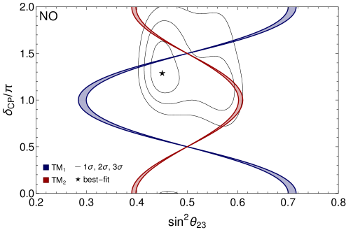
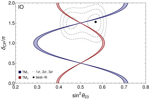
Figure 2.1: $\delta_{\rm CP}$ plotted against $\sin^{2}\theta_{23}$ within TM₁ and TM₂ models using Eqs. (2.45) and (2.46) and with the NuFit 5.2 oscillation data [19, 20] from Tab. 1.1. The $1\sigma$, $2\sigma$, $3\sigma$ regions (also in next figures) were derived from $\chi^{2}$ tables (NuFit 5.2 data files [160] with SK atmospheric data) for corresponding two-dimensional projections of the global analysis, minimized for a given mass ordering. The blue (red) shaded region represents TM₁ (TM₂) model predictions for $\sin^{2}\theta_{13}$ in the $3\sigma$ range.

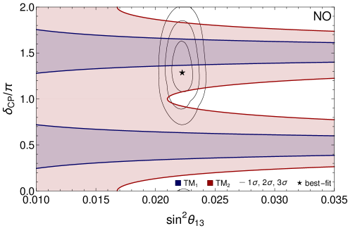
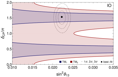
Figure 2.2: $\delta_{\rm CP}$ plotted against $\sin^{2}\theta_{13}$ within TM₁ and TM₂ models using Eqs. (2.45) and (2.46) and with the NuFit 5.2 oscillation data [19, 20] from Tab. 1.1. The blue (red) shaded region represents TM₁ (TM₂) model predictions for $\sin^{2}\theta_{23}$ in the $3\sigma$ range.

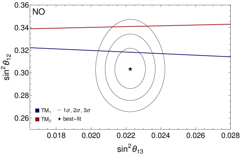
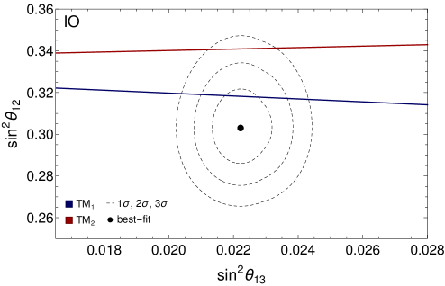
Figure 2.3: $\sin^{2}\theta_{12}$ plotted against $\sin^{2}\theta_{13}$ for TM₁ and TM₂ mixing [cf. Eqs. (2.45) and (2.46)] with the NuFit 5.2 oscillation data [19, 20].

The above discussion shows special cases of the TBM mixing, which can still be relevant for models with discrete flavor symmetries. Now, imposing sufficient corrections to the other fixed mixing schemes like BM, GR, and HG we can make them consistent with observed data [135, 161, 162, 163, 164, 165, 166]. The modified mixing matrix can be obtained by lowering the residual symmetry $G_{\nu}$ for the neutrino sector. This generates a correction matrix for these fixed mixing patterns. The general form of these corrections can be summarized as [133, 90, 167]

$$U=U_{e}^{\dagger}U_{0}U_{p},$$ (2.44)

where $U_{0}$ is the general form of the relevant fixed pattern mixing scheme mentioned in Eq. (1.9), $U_{e}$ is the generic correction matrix and $U_{p}$ is additional phase matrix contributing in the Dirac and Majorana phases mentioned in Eq. (1.1). These corrections help us to obtain interesting correlations among $\sin\theta_{12},\sin\theta_{23},\sin\theta_{13}$ and $\delta_{\rm CP}$ of PMNS mixing matrix [168]. In Tab. 2.2, we mention the typical predictions for TM₁ and TM₂ mixing matrices, including the Jarlskog invariant $J_{CP}=c_{12}s_{12}c_{23}s_{23}c_{13}^{2}s_{13}\sin\delta_{\rm CP}$ [169].

	TM1	TM2
$|U_{e2}|$	$\left|\frac{\cos\theta}{\sqrt{3}}\right|$	$\frac{1}{\sqrt{3}}$
$|U_{e3}|$	$\left|\frac{\sin\theta}{\sqrt{3}}\right|$	$\left|\frac{2\sin\theta}{\sqrt{6}}\right|$
$|U_{\mu 3}|$	$\left|\frac{\cos\theta}{\sqrt{2}}+\frac{\sin\theta}{\sqrt{3}}e^{-i\gamma}\right|$	$\left|-\frac{\cos\theta}{\sqrt{2}}-\frac{\sin\theta}{\sqrt{6}}e^{-i\gamma}\right|$
$\sin^{2}\theta_{12}$	$1-\frac{2}{3-\sin^{2}\theta}$	$\frac{1}{3-2\sin^{2}\theta}$
$\sin^{2}\theta_{13}$	$\frac{1}{3}\sin^{2}\theta$	$\frac{2}{3}\sin^{2}\theta$
$\sin^{2}\theta_{12}$	$\frac{1}{2}\left(1-\frac{\sqrt{6}\sin 2\theta\cos\gamma}{3-\sin^{2}\theta}\right)$	$\frac{1}{2}\left(1+\frac{\sqrt{3}\sin 2\theta\cos\gamma}{3-\sin^{2}\theta}\right)$
$J_{CP}$	$-\frac{1}{6\sqrt{6}}\sin 2\theta\sin\gamma$	$-\frac{1}{6\sqrt{3}}\sin 2\theta\sin\gamma$
$\sin\delta_{\rm CP}$	-$\frac{(5+\cos 2\theta)\sin\gamma}{\sqrt{(5+\cos 2\theta)^{2}-24\sin^{2}2\theta\cos^{2}\gamma}}$	-$\frac{(2+\cos 2\theta)\sin\gamma}{\sqrt{(2+\cos 2\theta)^{2}-3\sin^{2}2\theta\cos^{2}\gamma}}$

Table 2.2: Mixing parameters in the TM₁ and TM₂ scenarios. For more details, see  Ref. [168]. The elements $U_{e2},U_{e3},U_{\mu 3}$ are defined in Fig. 1.4.

The correlations among the neutrino mixing angles ($\theta_{23},\theta_{12},\theta_{13}$) and phase ($\delta_{\rm CP}$) for TM₁ and TM₂ respectively can be written as [170]

$$\mbox{TM}_{1} : s_{12}^{2}=\frac{1-3s_{13}^{2}}{3-3s_{13}^{2}},~{}~{}~{}\cos\delta_{\rm CP}=\frac{(1-5s_{13}^{2})(2s_{23}^{2}-1)}{4s_{13}s_{23}\sqrt{2(1-3s_{13}^{2})(1-s_{23}^{2})}},$$ (2.45)

$$\mbox{TM}_{2} : s_{12}^{2}=\frac{1}{3-3s_{13}^{2}},~{}~{}~{}\cos\delta_{\rm CP}=-\frac{(2-4s_{13}^{2})(2s_{23}^{2}-1)}{4s_{13}s_{23}\sqrt{(2-3s_{13}^{2})(1-s_{23}^{2})}}.$$ (2.46)

This helps us illuminate the feasibility of these models in the context of present neutrino oscillation data. In this regard, following Eqs. (2.45) and (2.46), we have plotted correlations in $\sin^{2}\theta_{23}-\delta_{\rm CP}$, $\sin^{2}\theta_{13}-\delta_{\rm CP}$ and $\sin^{2}\theta_{12}-\sin^{2}\theta_{13}$ planes for both NO and IO in Figs. 2.1, 2.2 and 2.3, respectively. In these plots we have also shown the 1$\sigma$, 2$\sigma$, 3$\sigma$ allowed regions of neutrino oscillation data, based on the two degrees of freedom (2 dof) tabularized data given in Ref. [160]. The best-fit values are denoted by $\star$ ($\bullet$) for NO (IO). The $\sin^{2}\theta_{23}-\delta_{\rm CP}$ correlation plotted in Fig. 2.1 is important because of the existing ambiguities on octant of $\theta_{23}$ (i.e., whether it is $\theta_{23}>45^{\circ}$ or $\theta_{23}<45^{\circ}$ ) and precise value of $\delta_{\rm CP}$. Here the blue and red shaded regions represent the predicted correlation of $\theta_{23}$ and $\delta_{\rm CP}$ for TM₁ and TM₂ for 3$\sigma$ allowed range of $\sin^{2}\theta_{13}$. For correlations $\sin^{2}\theta_{13}-\delta_{\rm CP}$ in Fig. 2.2, the spreading of the shaded region depends on the 3$\sigma$ allowed range of $\theta_{23}$. In Fig. 2.3, the $\sin^{2}\theta_{12}-\sin^{2}\theta_{13}$ correlations for TM₁ and TM₂ mixing schemes yield tight constraints on the allowed ranges of $\sin^{2}\theta_{12}$: NO (IO) $0.3168-0.3195~{}(0.3167-0.3195)$ for TM₁ and $0.3405-0.3413~{}(0.3405-0.3413)$ for TM₂. Furthermore, the $\sin^{2}\theta_{12}$ prediction for the TM₂ mixing lies at the edge of the 3$\sigma$ allowed region. Thus, a precise measurement of $\sin^{2}\theta_{12}$ can potentially rule out the TM₂ mixing scheme and corresponding flavor symmetric models.

Explicit models to obtain TM₁ and TM₂ mixing can be found on various occasions in the literature [171, 172, 144, 170]. We present examples of such models for TM₁ and TM₂ mixing with $A_{4}$ non-Abelian discrete flavor symmetry. Here, we will present an example of the TM₁ mixing in the context of a hybrid flavor symmetric scoto-seesaw scenario (FSS) [173, 174] where effective neutrino mass is generated via both type-I seesaw and scotogenic contributions. In the next subsection, we will discuss various ways to obtain light neutrino masses. The particle content of our model and charge assignment under different symmetries are shown in Tab. 2.3. The role of each discrete symmetry, particle content and charge assignment in this table are described in detail in Refs. [173, 175].

Fields	$e_{R}$, $\mu_{R}$, $\tau_{R}$	$L_{\alpha}$	$H$	$N_{R}$	$f$	$\eta$	$\phi_{S}$	$\phi_{A}$	$\phi_{T}$	$\xi$
$A_{4}$	$1$ , $1^{\prime\prime}$ , $1^{\prime}$	$3$	$1$	$1$	$1$	$1$	$3$	$3$	3	$1^{\prime\prime}$
$Z_{4}$	$i$	$i$	$1$	$1$	$1$	$1$	$i$	$i$	$1$	$1$
$Z_{3}$	$\omega^{2}$	$\omega$	$1$	$\omega^{2}$	1	$1$	$\omega^{2}$	$\omega$	$\omega^{2}$	$1$
$Z_{2}$	$1$	$1$	$1$	$1$	$-1$	$1$	$1$	$1$	$1$	$-1$

Table 2.3: Field contents and transformation under the symmetries of our model. flavons field in second block of the table are introduced to implement the $A_{4}$ symmetry.

In this setup, the charged lepton Lagrangian can be written up to the leading order as

$$\mathcal{L}_{l} = \frac{y_{e}}{\Lambda}(\bar{L}\phi_{T})_{1}He_{R}+\frac{y_{\mu}}{\Lambda}(\bar{L}\phi_{T})_{1^{\prime}}H\mu_{R}+\frac{y_{\tau}}{\Lambda}(\bar{L}\phi_{T})_{1^{\prime\prime}}H\tau_{R}+h.c.,$$ (2.48)

$$= {\frac{y_{e}}{\Lambda}(\bar{L}_{1}\phi_{T_{1}}+\bar{L}_{2}\phi_{T_{3}}+\bar{L}_{3}\phi_{T_{2}})He_{R}+\frac{y_{\mu}}{\Lambda}(\bar{L}_{3}\phi_{T_{3}}+\bar{L}_{1}\phi_{T_{2}}+\bar{L}_{2}\phi_{T_{1}})H\mu_{R}}$$

$${+\frac{y_{\tau}}{\Lambda}(\bar{L}_{2}\phi_{T_{2}}+\bar{L}_{1}\phi_{T_{3}}+\bar{L}_{3}\phi_{T_{1}})H\tau_{R}}$$

where $\Lambda$ is the cut-off scale of the FSS model. $y_{e}$, $y_{\mu}$ and $y_{\tau}$ are the coupling constants. In Eq. (2.48), the terms in the first parenthesis represent products of two $A_{4}$ triplets forming a one-dimensional representation which further contract with 1, $1^{\prime\prime}$ and $1^{\prime}$ of $A_{4}$, corresponding to $e_{R}$, $\mu_{R}$ and $\tau_{R}$, respectively. Following multiplication rules given in A, the complete $A_{4}$ decomposition is written in Eq. (2.48). Now, when the flavon $\phi_{T}$ gets VEV in the direction $\langle\phi_{T}\rangle=(\langle\phi_{T_{1}}\rangle+\langle\phi_{T_{2}}\rangle+\langle\phi_{T_{3}}\rangle)^{T}=(v_{T},0,0)^{T}$, the charged lepton Lagrangian can be written as

$$\mathcal{L}_{l} = \frac{y_{e}}{\Lambda}\bar{L}_{1}v_{T}He_{R}+\frac{y_{\mu}}{\Lambda}\bar{L}_{2}v_{T}H\mu_{R}+\frac{y_{\tau}}{\Lambda}\bar{L}_{3}v_{T}H\tau_{R}.$$ (2.49)

Finally, when the SM Higgs field $h$ also gets non-zero VEV as $\langle h\rangle=v$, following Eq. (2.49), the diagonal charged lepton mass matrix can be written as

$$m_{l} = \frac{vv_{T}}{\Lambda}\begin{pmatrix}y_{e}&0&0\\ 0&y_{\mu}&0\\ 0&0&y_{\tau}\end{pmatrix}.$$ (2.50)

Now, the Lagrangian for neutrino mass contributions in FSS can be written as

$$\mathcal{L}=\frac{y_{N}}{\Lambda}(\bar{L}\phi_{S})_{1}\tilde{H}N_{R}+\frac{1}{2}M_{N}\bar{N}_{R}^{c}N_{R}+\frac{y_{s}}{\Lambda^{2}}(\bar{L}\phi_{A})_{1^{\prime}}\xi i\sigma_{2}\eta^{*}f+\frac{1}{2}M_{f}\bar{f}^{c}f+h.c.,$$ (2.51)

where $y_{N}$ and $y_{s}$ are the coupling constant and $M_{N}$ is the Majorana mass of the right-handed neutrino $N_{R}$ while $M_{f}$ is the mass of the fermion $f$. Again, following A and Eq. (2.51), the $A_{4}$ decomposition for the contribution to the neutrino sector can be written as

$$\mathcal{L} = \frac{y_{N}}{\Lambda}(\bar{L}_{1}\phi_{S_{1}}+\bar{L}_{2}\phi_{S_{3}}+\bar{L}_{3}\phi_{S_{2}})\tilde{H}N_{R}+\frac{1}{2}M_{N}\bar{N}_{R}^{c}N_{R}$$ (2.52)

$$+\frac{y_{s}}{\Lambda^{2}}(\bar{L}_{3}\phi_{A_{3}}+\bar{L}_{1}\phi_{A_{2}}++\bar{L}_{2}\phi_{A_{1}})\xi i\sigma_{2}\eta^{*}f+\frac{1}{2}M_{f}\bar{f}^{c}f+h.c.,$$

$$= \frac{y_{N}}{\Lambda}(\bar{L}_{2}v_{S}-\bar{L}_{3}v_{S})\tilde{H}N_{R}+\frac{1}{2}M_{N}\bar{N}_{R}^{c}N_{R}+\frac{y_{s}}{\Lambda^{2}}(\bar{L}_{1}v_{A}+2\bar{L}_{2}v_{A})\xi i\sigma_{2}\eta^{*}f+\frac{1}{2}M_{f}\bar{f}^{c}f+h.c.$$ (2.53)

In the above Lagrangian, we put VEVs of $\phi_{S}$, $\phi_{A}$ and $\xi$ in directions $\langle\phi_{S}\rangle=(\langle\phi_{S_{1}}\rangle,\langle\phi_{S_{2}}\rangle,\langle\phi_{S_{3}}\rangle)^{T}=(0,-v_{S},v_{S})^{T}$, $\langle\phi_{A}\rangle=(\langle\phi_{A_{1}}\rangle,\langle\phi_{A_{2}}\rangle,\langle\phi_{A_{3}}\rangle)^{T}=(2v_{A},v_{A},0)^{T}$ and $v_{\xi}$, respectively, getting the appropriate flavor structure. Following Eq. (2.51), the Yukawa coupling for Dirac neutrinos and scotogenic contributions can be written as

$$Y_{N}=(Y_{N}^{e},Y_{N}^{\mu},Y_{N}^{\tau})^{T}=(0,y_{N}\frac{v_{S}}{\Lambda},-y_{N}\frac{v_{S}}{\Lambda})^{T},$$ (2.54)

$$Y_{F}=(Y_{F}^{e},Y_{F}^{\mu},Y_{F}^{\tau})^{T}=(y_{s}\frac{v_{\xi}}{\Lambda}\frac{v_{A}}{\Lambda},y_{s}\frac{v_{\xi}}{\Lambda}\frac{2v_{A}}{\Lambda},0)^{T}\equiv(\kappa,2\kappa,0)^{T}.$$ (2.55)

Finally, with the above Yukawa couplings, the total effective light neutrino mass matrix (with both type-I and scotogenic contributions) is given by

$$m_{\nu} = -\frac{v^{2}}{M_{N}}Y_{N}^{i}Y_{N}^{j}+\mathcal{F}(m_{\eta_{R}},m_{\eta_{I}},M_{f})M_{f}Y_{f}^{i}Y_{f}^{j}$$ (2.56)

$$= \begin{pmatrix}b&2b&0\\ 2b&-a+4b&a\\ 0&a&-a\end{pmatrix},$$ (2.57)

where $a=y_{N}^{2}\frac{v^{2}}{M_{N}}\frac{v_{S}^{2}}{\Lambda^{2}},b=y_{s}^{2}\frac{v_{\xi}^{2}}{\Lambda^{2}}\frac{v_{A}^{2}}{\Lambda^{2}}\mathcal{F}(m_{\eta_{R}},m_{\eta_{I}},M_{f})M_{f}=\kappa^{2}\mathcal{F}(m_{\eta_{R}},m_{\eta_{I}},M_{f})M_{f}$ and the loop function $\mathcal{F}$ is written as

$$\mathcal{F}(m_{\eta_{R}},m_{\eta_{I}},M_{f})=\frac{1}{32\pi^{2}}\Big{[}\frac{m_{\eta_{R}}^{2}\log\Big{(}M_{f}^{2}/m_{\eta_{R}}^{2}\Big{)}}{M_{f}^{2}-m_{\eta_{R}}^{2}}-\frac{m_{\eta_{I}}^{2}\log\Big{(}M_{f}^{2}/m_{\eta_{I}}^{2}\Big{)}}{M_{f}^{2}-m_{\eta_{I}}^{2}}\Big{]},$$ (2.58)

with $m_{\eta_{R}}$ and $m_{\eta_{I}}$ being the masses of the neutral component of $\eta$. The total mass matrix $m_{\nu}$ therefore can be diagonalized by a mixing matrix of TM₁ mixing pattern given by

$$U=\begin{pmatrix}\sqrt{\frac{2}{3}}&\frac{\cos\theta}{\sqrt{3}}&\frac{e^{-i\psi}\sin\theta}{\sqrt{3}}\\ -\frac{1}{\sqrt{6}}&\frac{\cos\theta}{\sqrt{3}}+\frac{e^{i\psi}\sin\theta}{\sqrt{2}}&-\frac{\cos\theta}{\sqrt{2}}+\frac{e^{-i\psi}\sin\theta}{\sqrt{3}}\\ -\frac{1}{\sqrt{6}}&\frac{\cos\theta}{\sqrt{3}}-\frac{e^{i\psi}\sin\theta}{\sqrt{2}}&\frac{\cos\theta}{\sqrt{2}}+\frac{e^{-i\psi}\sin\theta}{\sqrt{3}}\end{pmatrix}U_{M}$$ (2.59)

where $U_{M}$ is the Majorana phase matrix defined in Eq. (1.1). The correlation among the oscillation parameters is given in Eq. (2.45). In literature, the TM₁ mixing has been reproduced using various discrete groups such as $S_{4}$ in the context of type-I or type-II seesaw scenarios [144, 170, 176, 177].

To reproduce the TM₂ mixing, we adopt a modified version of the Altarelli-Feruglio (AF) model [114, 155]. In this scenario, light neutrino masses are generated completely via type-I seesaw, and hence three copies of RHNs are included which we consider to be a triplet under $A_{4}$. With the involvement of the $A_{4}$ flavons $\phi_{s},\phi_{T}$ (both triplet) and $\xi$ (singlet) one can obtain the TBM mixing. Now to accommodate nonzero $\theta_{13}$, $\delta_{\rm CP}$, the desired TM₂ mixing can be achieved in the involvement of one additional flavon $\xi^{\prime}$ ($1^{\prime}$ under $A_{4}$) which contributes to the right-handed neutrino mass. In addition to the $A_{4}$ discrete symmetry, we also consider a $Z_{3}$ symmetry which forbids the exchange of $\phi_{s}$ and $\phi_{T}$ in the Lagrangian. The complete particle content and their transformations under the symmetries are given in Tab. 2.4.

Fields	$e_{R}$, $\mu_{R}$, $\tau_{R}$	$L$	$N_{R}$	$H$	$\phi_{S}$	$\phi_{T}$	$\xi$	$\xi^{\prime}$
$SU(2)$	1	2	1	2	1	1	1	1
$A_{4}$	1,$1^{\prime\prime}$, $1^{\prime}$	3	3	1	3	3	1	$1^{\prime}$
$Z_{3}$	$\omega$	$\omega$	$\omega^{2}$	1	$\omega^{2}$	1	$\omega^{2}$	$\omega^{2}$

Table 2.4: Transformation of the fields needed to realize the $TM_{2}$ mixing . Here $\omega$ is the third root of unity. $\xi^{\prime}$ is essential to generate non-zero $\theta_{13}$.

Here we have considered the VEVs for the scalar fields as $\langle\phi_{S}\rangle=(v_{S},v_{S},v_{S})^{T}$, $\langle\phi_{T}\rangle=(v_{T},0,0)^{T}$, $\langle\xi\rangle=v_{\xi}$, $\langle\xi^{\prime}\rangle=v_{\xi^{\prime}}$  [114, 178, 155]. In Tab. 2.4, $H$ is the $SU(2)$ Higgs doublet (with VEV $v$) and singlet under $A_{4}$. Now, with the symmetries and particle content present in Tab. 2.4, the Lagrangian for the charged leptons can be written as

$${\cal{L}}_{CL} = \big{(}{y}_{e}(L{\phi_{T}})_{1}e_{R}+{y}_{\mu}(L{\phi_{T}})_{1^{\prime}}\mu_{R}+{y}_{\tau}(L{\phi_{T}})_{1^{\prime\prime}}\tau_{R}\big{)}\frac{H}{\Lambda},$$ (2.60)

where $\Lambda$ is the cutoff scale of the theory and $y_{e},y_{\mu},y_{\tau}$ are the corresponding coupling constants. Note that each term in the first parentheses represents products of two $A_{4}$ triplets $L,\phi_{T}$ which further contracts with $e_{R}$, $\mu_{R}$, $\tau_{R}$, which are charged under $A_{4}$ as $1,1^{\prime\prime}$ and $1^{\prime}$, respectively. Following the prescription given in Eq. (2.48), the charged lepton mass matrix can be obtained as

$$M_{\ell} = \frac{vv_{T}}{\Lambda}\begin{pmatrix}y_{e}&0&0\\ 0&y_{\mu}&0\\ 0&0&y_{\tau}\end{pmatrix}.$$ (2.61)

In the presence of the $A_{4}$ flavons $\phi_{s},\xi,\xi^{\prime}$ (with VEV $\langle\phi_{S}\rangle=(v_{S},v_{S},v_{S})^{T}$, $\langle\xi\rangle=v_{\xi}$, and  $\langle\xi^{\prime}\rangle=v_{\xi^{\prime}}$), the Lagrangian for the neutrino sector can be written as

$${\cal{L}}_{\nu} = y(LN_{R})H+(x_{A}\xi+x_{B}\phi_{S}+x_{N}\xi^{\prime})\overline{N^{c}}_{R}N_{R},$$ (2.63)

$$= y(L_{1}N_{R_{1}}+L_{2}N_{R_{3}}+L_{3}N_{R_{2}})H+x_{A}(\overline{N^{c}}_{R_{1}}N_{R_{1}}+\overline{N^{c}}_{R_{2}}N_{R_{3}}+\overline{N^{c}}_{R_{3}}N_{R_{2}})$$

$$+x_{B}\phi_{S_{1}}(2\overline{N^{c}}_{R_{1}}N_{R_{1}}-\overline{N^{c}}_{R_{2}}N_{R_{3}}-\overline{N^{c}}_{R_{3}}N_{R_{2}})/3+x_{B}\phi_{S_{1}}(2\overline{N^{c}}_{R_{1}}N_{R_{1}}-\overline{N^{c}}_{R_{2}}N_{R_{3}}-\overline{N^{c}}_{R_{3}}N_{R_{2}})/3$$

$$+x_{B}\phi_{S_{3}}(2\overline{N^{c}}_{R_{3}}N_{R_{3}}-\overline{N^{c}}_{R_{1}}N_{R_{2}}-\overline{N^{c}}_{R_{2}}N_{R_{1}})/3+x_{N}\xi^{\prime}(\overline{N^{c}}_{R_{2}}N_{R_{2}}+\overline{N^{c}}_{R_{1}}N_{R_{3}}+\overline{N^{c}}_{R_{3}}N_{R_{1}})$$

where $y$, $x_{A}$, $x_{B}$ are the coupling constants. After spontaneous breaking of electroweak and flavor symmetries, we obtain the Dirac and Majorana mass matrices as

$$m_{D}=yv\begin{pmatrix}1&0&0\\ 0&0&1\\ 0&1&0\end{pmatrix},M_{R}=\begin{pmatrix}a+2b/3&-b/3&-b/3\\ -b/3&2b/3&a-b/3\\ -b/3&a-b/3&2b/3\end{pmatrix}+\begin{pmatrix}0&0&d\\ 0&d&0\\ d&0&0\end{pmatrix},$$ (2.64)

where $a=2x_{A}v_{\xi},b=2x_{B}v_{S}$ and $d=2x_{N}v_{\xi^{\prime}}$. The mass matrices for Dirac, and Majorana neutrinos are obtained from the Lagrangian written in Eqs.(2.60) and (2.63) following the $A_{4}$ multiplication rules given in A. The light neutrino mass matrix can be obtained through the type-I seesaw mechanism using the relation $M_{\nu}=-M_{D}^{T}M_{R}^{-1}M_{D}$. After diagonalizing $M_{\nu}$ with the tribimaximal mixing matrix $U_{\rm TB}$ we find,

$$M^{\prime}_{\nu} = U^{T}_{\rm TB}M_{\nu}U_{\rm TB}$$ (2.65)

$$= y^{2}v^{2}\begin{pmatrix}\frac{2(a+b)-d}{2(a^{2}-b^{2}-ad+d^{2})}&0&\frac{-\sqrt{3}d}{2(a^{2}-b^{2}-ad+d^{2})}\\ 0&\frac{1}{a+d}&0\\ \frac{-\sqrt{3}d}{2(a^{2}-b^{2}-ad+d^{2})}&0&\frac{2(b-a)+d}{2(a^{2}-b^{2}-ad+d^{2})}\end{pmatrix}.$$ (2.66)

The above matrix is diagonal for $d=0$ (contribution corresponding to $\xi^{\prime}$). Therefore, the light neutrino mass matrix will no longer be diagonalized by $U_{TB}$ and a further rotation in the 13-plane can diagonalize $m^{\prime}_{\nu}$ given in Eq. (2.66). So the final diagonalizing matrix for the light neutrino mass matrix can be written as

$$U = \begin{pmatrix}\sqrt{\frac{2}{3}}&\frac{1}{\sqrt{3}}&0\\ -\frac{1}{\sqrt{6}}&\frac{1}{\sqrt{3}}&-\frac{1}{\sqrt{2}}\\ -\frac{1}{\sqrt{6}}&\frac{1}{\sqrt{3}}&\frac{1}{\sqrt{2}}\end{pmatrix}.\begin{pmatrix}\cos\theta&0&\sin\theta e^{-i\psi}\\ 0&1&0\\ -\sin\theta e^{i\psi}&0&\cos\theta\end{pmatrix}U_{M},$$ (2.67)

$$= \begin{pmatrix}\sqrt{\frac{2}{3}}\cos\theta&\frac{1}{\sqrt{3}}&\sqrt{\frac{2}{3}}e^{i\psi}\sin\theta\\ -\frac{\cos\theta}{\sqrt{6}}+\frac{e^{i\psi}\sin\theta}{\sqrt{2}}&\frac{1}{\sqrt{3}}&-\frac{\cos\theta}{\sqrt{2}}-\frac{e^{i\psi}\sin\theta}{\sqrt{6}}\\ -\frac{\cos\theta}{\sqrt{6}}-\frac{e^{i\psi}\sin\theta}{\sqrt{2}}&\frac{1}{\sqrt{3}}&\frac{\cos\theta}{\sqrt{2}}-\frac{e^{i\psi}\sin\theta}{\sqrt{6}}\end{pmatrix}U_{M},$$

where, as in the TM₁ case, $U_{M}$ is the Majorana phase matrix defined in Eq. (1.1). The structure of the mixing matrix coincides with the TM₂ mixing obtained in the context of $A_{4}$ non-Abelian discrete flavor symmetry.

As mentioned earlier, the mixing matrix in Eq. (1.18) and the corresponding mass matrix Eq. (1.14) obeys the underlying $\mu-\tau$ symmetry (also known as the $\mu-\tau$ permutation symmetry). As this feature is outdated now for obvious reasons, there is another class of flavor CP model known as $\mu-\tau$ reflection symmetry [96]. This symmetry can be expressed as the transformation:

$$\nu_{e}\rightarrow\nu_{e}^{C},~{}\nu_{\mu}\rightarrow\nu_{\tau}^{C},~{}\nu_{\tau}\rightarrow\nu_{\mu}^{C}$$ (2.68)

where ‘C’ stands for the charge conjugation of the corresponding neutrino field under which the neutrino mass term remains unchanged. The scheme leads to the predictions $\theta_{23}=45^{\circ}$, $\delta_{\rm CP}=90^{\circ}~{}{\rm or}~{}270^{\circ}$. This mixing scheme is still experimentally viable [20]. Under the discussed $\mu-\tau$ symmetry, the elements of the lepton mixing matrix satisfy

$$|U_{\mu i}|=|U_{\tau i}|~{}~{}~{}~{}~{}{\rm where}~{}~{}~{}{i=1,2,3}.$$ (2.69)

Such a mixing scheme is also known as cobimaximal (CBM) mixing scheme [179]. Eq. (2.69) indicates that the moduli of $\mu$ and $\tau$ flavor elements of the $3\times 3$ neutrino mixing matrix are equal. With these constraints, the neutrino mixing matrix can be parametrized as [180, 181]

$$U_{0} = \left(\begin{array}[]{ccc}u_{1}&u_{2}&u_{3}\\ v_{1}&v_{2}&v_{3}\\ v^{*}_{1}&v^{*}_{2}&v^{*}_{3}\end{array}\right),$$ (2.73)

where the entries in the first row, $u_{i}$’s are real (and non-negative) with trivial (vanishing) values of the Majorana phases. Here $v_{i}$ satisfies the orthogonality condition ${\rm Re}(v_{j}v_{k}^{*})=\delta_{jk}-u_{k}u_{k}$. In Ref. [181] it was argued that the mass matrix leading to the mixing matrix given in Eq. (2.73) can be written as

$${M}_{0} = \left(\begin{array}[]{ccc}a&d&d^{*}\\ d&c&b\\ d^{*}&b&c^{*}\end{array}\right),$$ (2.77)

where $a,b$ are real and $d,c$ are complex parameters. As a consequence of the symmetry given in Eqs.(2.69)-(2.77), we obtain the predictions for maximal $\theta_{23}=45^{\circ}$ and $\delta_{\rm CP}=90^{\circ}~{}{\rm or}~{}270^{\circ}$ in the basis where the charged leptons are considered to be diagonal. This scheme, however, still leaves room for nonzero $\theta_{13}$. Realization of such a mixing pattern is possible with various discrete flavor symmetries ($A_{4},\Delta(27)$, etc.), for example, see Refs. [182, 183, 184, 185, 186].

Earlier, we mentioned that fixed mixing schemes such as BM, TBM, GR, HG are ruled out and require specific corrections to accommodate non-zero $\theta_{13}$ and $\delta_{\rm CP}$. These corrections can also provide a possible deviation from $\theta_{23}=45^{\circ}$. For example, to achieve experimentally viable TM₁ and TM₂ mixing, we have shown instances where additional contribution to the neutrino sector over TBM mixing generates necessary corrections. However, this can be achieved in various ways. A correction in the charged lepton sector is one such possibility. This can be achieved by additional non-trivial contribution in the charged lepton sector  [150].

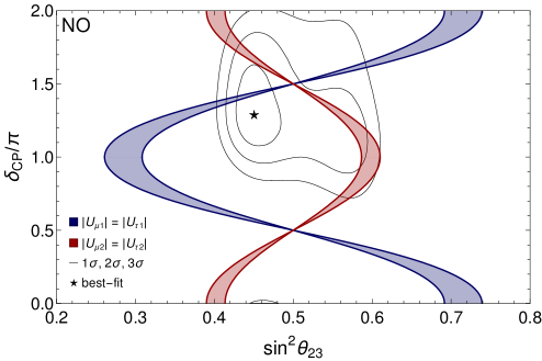
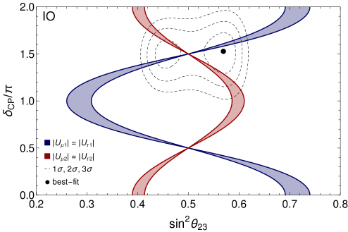
Figure 2.4: $\delta_{\rm CP}$ plotted against $\sin^{2}\theta_{23}$ within partial $\mu-\tau$ reflection symmetry predictions (Eqs. (2.78) and (2.79)) and the NuFit 5.2 oscillation data [19, 20]. The blue (red) shaded region represents $|U_{\mu 1}|=|U_{\tau 1}|$ ($|U_{\mu 2}|=|U_{\tau 2}|$) model predictions with $\sin^{2}\theta_{12}$ and $\sin^{2}\theta_{13}$ in the $3\sigma$ range.

Note that the most recent best-fit values for $\theta_{23}$ (Tab. 1.1) prefer lower octant ($\theta_{23}<45^{\circ}$) for NO and upper octant ($\theta_{23}>45^{\circ}$) for IO. Given this, it seems well motivated to introduce partial $\mu-\tau$ reflection symmetry, for which the $\delta_{\rm CP}$ and $\theta_{23}$ are not fixed but correlated [187]

$$|U_{\mu 1}|=|U_{\tau 1}| : ~{}~{}~{}\cos\delta_{\rm CP}=\frac{(c_{23}^{2}-s_{23}^{2})(c_{12}^{2}s_{13}^{2}-s_{12}^{2})}{4c_{12}s_{12}c_{23}s_{23}s_{13}},$$ (2.78)

$$|U_{\mu 2}|=|U_{\tau 2}| : ~{}~{}~{}\cos\delta_{\rm CP}=\frac{(c_{23}^{2}-s_{23}^{2})(c_{12}^{2}-s_{12}^{2}s_{13}^{2})}{4c_{12}s_{12}c_{23}s_{23}s_{13}}.$$ (2.79)

The $\delta_{\rm CP}-\theta_{23}$ correlations in Eqs. (2.78) and (2.79) for the partial $\mu-\tau$ reflection symmetry ($|U_{\mu 1}|=|U_{\tau 1}|$ , $|U_{\mu 2}|=|U_{\tau 2}|$) are given in Fig. 2.4. These correlations partially overlap the $1\sigma$, $2\sigma$, $3\sigma$ regions but do not include the best-fit values.

A similar investigation of partial $\mu-\tau$ reflection symmetry can also be performed for the 3+1 neutrino mixing scheme, denoted as (3+1)$\nu$, leading to the $\delta_{\rm CP}/\theta_{23}$ correlations as given below [182]

$$|U_{\mu 1}|=|U_{\tau 1}| : ~{}~{}\cos\delta_{\rm CP}=\frac{(a_{1}^{2}+b_{1}^{2})-(c_{1}^{2}+d_{1}^{2})}{2(c_{1}d_{1}-a_{1}b_{1})}$$ (2.80)

$$|U_{\mu 2}|=|U_{\tau 2}| : ~{}~{}\cos\delta_{\rm CP}=\frac{(a_{2}^{2}+b_{2}^{2})-(c_{2}^{2}+d_{2}^{2})}{2(a_{2}b_{2}-c_{2}d_{2})}$$ (2.81)

$$|U_{\mu 3}|=|U_{\tau 3}| : ~{}~{}\cos\delta_{\rm CP}=\frac{(a_{3}^{2}+b_{3}^{2})-(c_{3}^{2}+d_{3}^{2})}{2(a_{3}b_{3}-c_{3}d_{3})}$$ (2.82)

$${|U_{\mu 4}|=|U_{\tau 4}|} : ~{}~{}{\tan^{2}\theta_{24}=\sin^{2}\theta_{34}}$$ (2.83)

where

$$a_{1} =c_{12}s_{13}s_{23}s_{24}s_{34}-c_{12}c_{23}c_{34}s_{13}, b_{1} =c_{34}s_{12}s_{23}-c_{12}c_{13}c_{24}s_{14}s_{34}+c_{23}s_{12}s_{24}s_{34},$$ (2.84)

$$c_{1} =c_{23}c_{24}s_{12}+c_{12}c_{13}s_{14}s_{24}, d_{1} =c_{12}c_{24}s_{13}s_{23},$$

$$a_{2} =c_{12}(c_{34}s_{23}+c_{23}s_{24}s_{34})+s_{12}c_{13}c_{24}s_{14}s_{34}, b_{2} =s_{12}(s_{13}s_{23}s_{24}s_{34}-c_{23}c_{34}s_{13}),$$

$$c_{2} =c_{12}c_{23}c_{24}-s_{12}c_{13}s_{14}s_{24}, d_{2} =s_{12}c_{24}s_{13}s_{23},$$

$$a_{3} =c_{13}(c_{23}c_{34}-s_{23}s_{24}s_{34}), b_{3} =c_{24}s_{13}s_{14}s_{34},$$

$$c_{3} =s_{13}s_{14}s_{24}, d_{3} =c_{13}c_{24}s_{23}.$$

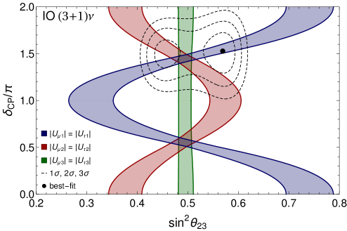
Figure 2.5: $\delta_{\rm CP}$ plotted against $\sin^{2}\theta_{23}$ in the (3+1)$\nu$ case within partial $\mu-\tau$ reflection symmetry scenario [182] and NuFit 5.2 (with SK atmospheric) oscillation data [19, 20]. The blue, red, green regions represent $|U_{\mu 1}|=|U_{\tau 1}|$ , $|U_{\mu 2}|=|U_{\tau 2}|$, $|U_{\mu 3}|=|U_{\tau 3}|$ symmetry predictions respectively. The $\sin^{2}\theta_{12}$ and $\sin^{2}\theta_{13}$ vary in $3\sigma$ range (Tab. 1.1) while the (3+1)$\nu$ oscillation parameters ($\theta_{14},\theta_{24},\theta_{34}$) vary in representative $3\sigma$ ranges given in Tab. I of Ref. [182] ($\theta_{14}:4^{\circ}-10^{\circ}$, $\theta_{24}:5^{\circ}-10^{\circ}$, $\theta_{34}:0^{\circ}-11^{\circ}$, $\delta_{14}=\delta_{24}=0^{\circ}$).

The results for the (3+1)$\nu$ scenario are gathered in Fig. 2.5. From the overlapped regions in Fig. 2.5, it is clear that if we demand a total $\mu-\tau$ reflection symmetry, i.e., $|U_{\mu i}|=|U_{\tau i}|$ for all four columns then the atmospheric mixing angle $\theta_{23}$ is restricted within a narrow region around $45^{\circ}$ and the Dirac CP phase is also restricted around the maximal CP violating values. Since the present best fit values for $\theta_{23}$ clearly favors a deviation from $45^{\circ}$ (see Fig. 1.1), a partial $\mu-\tau$ reflection symmetry in the (3+1)$\nu$ scenario may accommodate appropriate deviation. From Fig. 2.5, we find that $\delta_{\rm CP}-\theta_{23}$ correlations are partly overlapping the ($1\sigma$, $2\sigma$ and $3\sigma$) $\delta_{\rm CP}-\theta_{23}$ regions for all three partial $\mu-\tau$ reflection symmetries but only for the $|U_{\mu 1}|=|U_{\tau 1}|$ symmetry, the $\delta_{\rm CP}-\theta_{23}$ correlation region includes the best-fit value for IO. In addition to this it is worth mentioning that the partial $\mu-\tau$ reflection symmetry in the fourth column ($|U_{\mu 4}|=|U_{\tau 4}|$) restricts $\theta_{34}$ within the range $4.9^{\circ}-9.8^{\circ}$ [182].

2.3   Flavor Symmetry and Neutrino Mass Models

Apart from the observed pattern of neutrino mixing, the origin of tiny neutrino mass is still unknown to us. Over decades, the exclusive evidence for non-zero neutrino masses stems solely from neutrino oscillation experiments, which are sensitive to the mass-squared differences and not to the absolute scale of neutrino masses (see Tab. 1.1). On the other hand, bounds on absolute neutrino masses come from cosmological surveys [188, 50] and the end-point spectrum of tritium beta decay. Combining all these results, we come to the neutrino mass ranges discussed in the Introduction, which are at the mili-electronvolt scale at the most. Based on the established neutrino mass spectrum, different models try to explain it. For a detailed discussion of many mechanisms to generate light neutrino masses, the readers are referred to Refs. [189, 190, 191, 192, 193, 194] and references therein. Here, we briefly mention a few of them that are frequently used in realistic flavor model building.

Seesaw models

One of the most popular ways to generate tiny neutrino mass is to start with the high scale suppressed lepton number violating Weinberg operator $HL^{T}LH/\Lambda$ mentioned earlier, which is non-renormalizable. This can give rise to various seesaw mechanisms such as type-I, type-II, type-III, inverse and linear seesaw  [195, 196, 197, 198, 199, 8, 193]. They can be embedded in the form of Eq. (1.21), see Ref. [200]. However, to elucidate the observed pattern of neutrino mixings, one must include additional ingredients such as discrete flavor symmetries. Examples of discrete flavor symmetric models for type-I, type-II, and inverse seesaw which are very efficient in explaining tiny mass as well as correct mixing as observed by the neutrino oscillation experiments can be found in Refs. [155, 156, 157, 201, 202, 203, 204, 205, 206, 207, 208, 209, 210, 211, 212, 213, 214, 215]. Based on their scale, these flavor symmetric seesaw mechanisms may include a wide range of phenomenological implications in lepton flavor violation, collider phenomenology or leptogenesis [216].

Radiative mass models

Another class of models that can be connected with flavor symmetries are radiative neutrino mass models in which masses of neutrinos are absent at the tree-level and are generated at 1- or higher-loop orders. These models explain the lightness of neutrino masses with sizable Yukawa couplings and suppression provided by the loop factor. A broad review of various radiative neutrino models can be found in Ref. [194]. The key feature of these models is that they can be verified experimentally because the masses of exotic particles that take part in the neutrino mass generation are in the TeV range, which the current colliders’ experiments can probe. Furthermore, these models may contribute to electric dipole moments, anomalous magnetic moments and meson decays, matter-antimatter asymmetry [194, 217, 218]. Most interestingly, some radiative models naturally incorporate potential DM candidates [219, 220]. Additional symmetries that explain tiny neutrino masses also stabilize the DM. On top of that, radiative neutrino mass models with discrete flavor symmetries can also explain the observed lepton mixing for obvious reasons, for instance, modular $S_{3}$ and $A_{4}$ [221, 222, 223, 224, 225].

Neutrino mass sum rules

Neutrino mass mechanisms augmented with discrete flavor symmetries predict a range of neutrino masses and mixings and can yield interesting correlations between several observables, such as leptonic mixing angles, phases, and neutrino masses. Models that have these features enhance the testability at neutrino experiments. Discrete flavor symmetric models can give rise to sum rules for neutrino mixing angles and masses. The mixing sum rules relate the leptonic mixing angles to the Dirac CP-violating phase $\delta_{\rm CP}$ [226, 227, 145, 228]. For example, considering appropriate deviations, the approximate mixing sum rules can be written as  [229, 230, 231]

$$\sin^{2}\theta_{12} \simeq \frac{1}{2}+\sin{\theta_{13}}\cos\delta,$$ (2.85)

$$\sin^{2}{\theta_{12}} \simeq \frac{1}{3}+\frac{2\sqrt{2}}{3}\sin{\theta_{13}}\cos\delta,$$ (2.86)

for BM and TBM mixing, respectively. For the implication of the mixing sum rules at the neutrino oscillation experiments, see Ref. [228]. On the other hand, the mass sum rules [232, 233, 234, 235, 236, 237], which describe the interrelation between the three complex neutrino eigenvalues are particularly important because of their substantial implication [238, 239, 240, 241] in the prediction of the effective mass parameter ($m_{\beta\beta}$) appearing in the neutrinoless double beta decay described in Eq. (1.5). Theoretically, it is natural to wonder if these sum rules are related to residual or accidental symmetry. The neutrino mass sum rules can originate from discrete flavor symmetric models in which neutrino masses can arise from the aforementioned mass generation mechanisms. However, the most general mass sum rule can be written as [240]

$$A_{1}\tilde{m}_{1}^{p}e^{i\chi_{1}}+A_{2}\tilde{m}_{2}^{p}e^{i\chi_{2}}+A_{3}\tilde{m}_{3}^{p}e^{i\chi_{3}}=0,$$ (2.87)

where $\tilde{m_{i}}$ are three complex mass eigen values, $p\neq 0,\chi_{1}\in[0,2\pi],A_{i}>0$. Here $A_{i}$ and $\chi_{i}$ stand for appropriate complex coefficients and phase factors (without the Majorana phases). The power $q$ of the complex mass eigenvalues characterizes the sum rule. For example, a simple sum rule can be obtained when a type-I seesaw mass mechanism is augmented by $A_{5}$ non-Abelian discrete flavor symmetry leading to  [162]

$$\frac{1}{\tilde{m}_{1}}+\frac{1}{\tilde{m}_{2}}=\frac{1}{\tilde{m}_{3}}.$$ (2.88)

Comparing Eq. (2.87) and Eq. (2.88) we find that $A_{i}=1,\chi_{1,2}=0,\chi_{3}=\pi$ and $p=-1$. Such mass sum rules (i.e., when $p=-1$) are called inverse sum rules, obtained from a diverse combination of neutrino mass mechanisms and discrete flavor symmetries [114, 232, 242, 243, 155].

Sum Rule	Group	Seesaw Type
$\tilde{m}_{1}+\tilde{m}_{2}=\tilde{m}_{3}$	$A_{4}$[153, 244, 245, 246, 247, 248]; $S_{4}$[249]; $A_{5}$[73]	Weinberg
$\tilde{m}_{1}+\tilde{m}_{2}=\tilde{m}_{3}$	$\Delta(54)$[250]; $S_{4}$[251]	Type II
$\tilde{m}_{1}+2\tilde{m}_{2}=\tilde{m}_{3}$	$S_{4}$[252]	Type II
$2\tilde{m}_{2}+\tilde{m}_{3}=\tilde{m}_{1}$	$A_{4}$ [153, 113, 253, 254, 255, 256, 257, 258, 259, 245, 246, 247, 248, 114, 234]	Weinberg
	$S_{4}$[128, 260]; $T^{\prime}$[261, 262, 263, 151, 264, 243]; $T_{7}$[265]
$2\tilde{m}_{2}+\tilde{m}_{3}=\tilde{m}_{1}$	$A_{4}$[266]	Type II
$\tilde{m}_{1}+\tilde{m}_{2}=2\tilde{m}_{3}$	$S_{4}$[267]	Dirac
$\tilde{m}_{1}+\tilde{m}_{2}=2\tilde{m}_{3}$	$L_{e}-L_{\mu}-L_{\tau}$[268]	Type II
$\tilde{m}_{1}+\frac{\sqrt{3}+1}{2}\tilde{m}_{3}=\frac{\sqrt{3}-1}{2}\tilde{m}_{2}$	$A_{5}^{\prime}$[269]	Weinberg
$\tilde{m}_{1}^{-1}+\tilde{m}_{2}^{-1}=\tilde{m}_{3}^{-1}$	$A_{4}$[153]; $S_{4}$[251, 244]; $A_{5}$[76, 162]	Type I
$\tilde{m}_{1}^{-1}+\tilde{m}_{2}^{-1}=\tilde{m}_{3}^{-1}$	$S_{4}$[251]	Type III
$2\tilde{m}_{2}^{-1}+\tilde{m}_{3}^{-1}=\tilde{m}_{1}^{-1}$	$A_{4}$[153, 270, 232, 271, 272, 273, 235, 242, 274, 275, 276, 277, 278, 114, 234]; $T^{\prime}$[243]	Type I
$\tilde{m}_{1}^{-1}+\tilde{m}_{3}^{-1}=2\tilde{m}_{2}^{-1}$	$A_{4}$[279, 280, 281]; $T^{\prime}$[282]	Type I
$\tilde{m}_{3}^{-1}\pm 2i\tilde{m}_{2}^{-1}=\tilde{m}_{1}^{-1}$	$\Delta(96)$[283]	Type I
$\tilde{m}_{1}^{1/2}-\tilde{m}_{3}^{1/2}=2\tilde{m}_{2}^{1/2}$	$A_{4}$[233]	Type I
$\tilde{m}_{1}^{1/2}+\tilde{m}_{3}^{1/2}=2\tilde{m}_{2}^{1/2}$	$A_{4}$[284]	Scotogenic
$\tilde{m}_{1}^{-1/2}+\tilde{m}_{2}^{-1/2}=2\tilde{m}_{3}^{-1/2}$	$S_{4}$[237]	Inverse

Table 2.5: Sum rules for the complex light neutrino mass eigenvalues $\tilde{m}_{i}$ defined in Eq. (2.87) obtained with various combinations of neutrino mass generation mechanisms and discrete flavor symmetries [236, 240, 241].

In Tab. 2.5, we have mentioned various simple sum rules for the complex light neutrino mass eigenvalues ($\tilde{m}_{i}$) obtained with combinations of neutrino mass generation mechanism and discrete flavor symmetries [236, 240, 241]. Similar but less simple mass sum rules can also be obtained for models with modular symmetry. The authors reported in Ref. [285] four different mass sum rules for models based on modular symmetries where a residual symmetry in the lepton sector is preserved. The reported sum rules (SR) within these modular invariance approaches (which also follow the most general form given in Eq. (2.87)) are called SR 1 (Case I and Case II), SR 2, SR 3, and SR 4 [285]. Studies show that these sum rules can not be conclusively connected to a particular mass generation mechanism, discrete symmetry, or any remnant symmetry in the lepton sector [286]. Rather, they are more connected to minimal breaking of the symmetries, which introduces a minimal number of parameters related to nonzero neutrino mass eigenvalues. However, the Majorana phases (connected with the complex mass eigenvalues $\tilde{m}_{i}$) also appear in the mass sum rules, making them ideal observable to test them in the neutrinoless double beta decay experiments. The occurrence of such sum rules severely constrains the prediction for $m_{\beta\beta}$, see Fig. 3.3 in Section 3.2. A detailed discussion of the role of individual sum rules can be found in Refs. [238, 236, 239, 240, 241, 286].

Flavor Models: Majorana vs Dirac neutrinos

While neutrino oscillation experiments are insensitive to the nature of neutrinos, experiments looking for lepton number violating signatures can probe the Majorana nature of neutrinos. Neutrinoless double beta decay is one such lepton number violating process which has been searched for at several experiments without any positive result so far but giving stricter bounds on the effective neutrino mass, as discussed in Chapter 1. Although negative results at neutrinoless double beta decay experiments do not prove that the light neutrinos are of Dirac nature, it is nevertheless suggestive enough to come up with scenarios predicting Dirac neutrinos with correct mass and mixing. There have been several proposals already that can generate tiny Dirac neutrino masses [287, 288, 289, 290, 291, 292]. In Refs. [293, 294, 295, 296], the authors showed that it is possible to propose various seesaw mechanisms (type-I, inverse and linear seesaw) for Dirac neutrinos with $A_{4}$ discrete flavor symmetry. Here the symmetry is chosen in such a way that it naturally explains the hierarchy among different terms in the neutrino mass matrix, contrary to the conventional seesaws where this hierarchy is ad-hoc.

Texture zeroes

When a flavor neutrino mass matrix contains zero elements, this is called a texture zeros mass matrix. Texture zeroes make the neutrino mass and mixing models simpler. Such constructions are interesting as they lead to a reduction of independent mass parameters in theory. There is a vast literature on the subject, e.g. see the list of references in the recent work [301].

In the three-generation scenario, the low energy Majorana neutrino mass matrix $M_{\nu}$ is a $3\times 3$ complex symmetric matrix having six independent elements given by

$$M_{\nu} = \begin{pmatrix}m_{ee}&m_{e\mu}&m_{e\tau}\\ m_{e\mu}&m_{\mu\mu}&m_{\mu\tau}\\ m_{e\tau}&m_{\mu\tau}&m_{\tau\tau}\\ \end{pmatrix}.$$ (2.89)

For three generations and one-zero textures, all six one-zero textures $G_{1}-G_{6}$ in Tab. 2.6 can accommodate the experimental data [302], see also Refs. [303, 304, 305].

$${\rm G}_{1}:\left(\begin{array}[]{*{20}{c}}0&\times&\times\\ -&\times&\times\\ -&-&\times\\ \end{array}\right),\quad{\rm G}_{2}:\left(\begin{array}[]{*{20}{c}}\times&0&\times\\ -&\times&\times\\ -&-&\times\\ \end{array}\right),\quad{\rm G}_{3}:\left(\begin{array}[]{*{20}{c}}\times&\times&0\\ -&\times&\times\\ -&-&\times\\ \end{array}\right),\quad$$

$${\rm G}_{4}:\left(\begin{array}[]{*{20}{c}}\times&\times&\times\\ -&0&\times\\ -&-&\times\\ \end{array}\right),\quad{\rm G}_{5}:\left(\begin{array}[]{*{20}{c}}\times&\times&\times\\ -&\times&0\\ -&-&\times\\ \end{array}\right),\quad{\rm G}_{6}:\left(\begin{array}[]{*{20}{c}}\times&\times&\times\\ -&\times&\times\\ -&-&0\\ \end{array}\right).$$

Table 2.6: Possible one-zero textures in the three-generation neutrino flavor scenario.

The crosses “$\times$” stand for the non-zero entries and "$-$" represent symmetric elements (the matrices are assumed to be symmetric). There are 15 possible two-zero textures categorised in different classes, as shown in Tab. 2.7.

$A_{1}$	$A_{2}$			$D_{1}$	$D_{2}$
$\left(\begin{array}[]{ccc}0&0&\times\\ 0&\times&\times\\ -&-&\times\end{array}\right)$	$\left(\begin{array}[]{ccc}0&\times&0\\ -&\times&\times\\ 0&-&\times\end{array}\right)$			$\left(\begin{array}[]{ccc}\times&\times&\times\\ -&0&0\\ -&0&\times\end{array}\right)$	$\left(\begin{array}[]{ccc}\times&\times&\times\\ -&\times&0\\ -&0&0\end{array}\right)$
$B_{1}$	$B_{2}$	$B_{3}$	$B_{4}$	$E_{1}$	$E_{2}$	$E_{3}$
$\left(\begin{array}[]{ccc}\times&\times&0\\ -&0&\times\\ 0&-&\times\end{array}\right)$	$\left(\begin{array}[]{ccc}\times&0&\times\\ 0&\times&\times\\ -&-&0\end{array}\right)$	$\left(\begin{array}[]{ccc}\times&0&\times\\ 0&0&\times\\ -&-&\times\end{array}\right)$	$\left(\begin{array}[]{ccc}\times&\times&0\\ -&\times&\times\\ 0&-&0\end{array}\right)$	$\left(\begin{array}[]{ccc}0&\times&\times\\ -&0&\times\\ -&-&\times\end{array}\right)$	$\left(\begin{array}[]{ccc}0&\times&\times\\ -&\times&\times\\ -&-&0\end{array}\right)$	$\left(\begin{array}[]{ccc}0&\times&\times\\ -&\times&0\\ -&0&\times\end{array}\right)$
$C$				$F_{1}$	$F_{2}$	$F_{3}$
$\left(\begin{array}[]{ccc}\times&\times&\times\\ -&0&\times\\ -&-&0\end{array}\right)$				$\left(\begin{array}[]{ccc}\times&0&0\\ 0&\times&\times\\ 0&-&\times\end{array}\right)$	$\left(\begin{array}[]{ccc}\times&0&\times\\ 0&\times&0\\ -&0&\times\end{array}\right)$	$\left(\begin{array}[]{ccc}\times&\times&0\\ -&\times&0\\ 0&0&\times\end{array}\right)$

Table 2.7: Possible two-zero textures in the three-generation neutrino flavor scenario.

The sum of crosses in each matrix in Tabs. 2.6 and 2.7 gives the number of independent parameters of 5(4) for textures with one (two) zeroes. Textures with more than two independent zeroes appear to be excluded by the experiments (three independent parameters are not enough to accommodate neutrino data).

In the $3\times 3$ scenario, among the 15 possible textures, only 7 are phenomenologically allowed [308, 309, 106]. In Ref. [310], nine patterns were compatible with data (two of them only marginally for considered experimental data). The results, in general, depend strongly on available data. After measurement of non-zero $\theta_{13}$, the updated analysis can be found in Refs. [311, 312, 313] and the number of viable textures have been reduced significantly, namely:

1. Class $A$ is allowed only for NH.

2. Class $B$ is allowed for both NH and IH. $B_{1}$ and $B_{4}$ predict negative values of $\cos\delta_{\rm CP}$ whereas the classes $B2$ and $B3$ predict positive values of $\cos\delta_{\rm CP}$. The textures $B1$ and $B3$ predict $\theta_{23}$ in the lower octant and the textures $B2$ and $B4$ predict $\theta_{23}$ in the upper octant for NH. The predictions are opposite for the IH.

3. Class $C$ class is allowed mainly in the IH. This class is marginally allowed in the NH when $\theta_{23}$ is close to $45^{\circ}$. In this class when $\theta_{23}<45^{\circ}$, one must have $-90^{\circ}<\delta_{\rm CP}<90^{\circ}$ and when $\theta_{23}>45^{\circ}$, one must have $90^{\circ}<\delta_{\rm CP}<270^{\circ}$.

4. The textures in the classes $D$, $E$ and $F$ are forbidden by the data.

In Ref. [108] numerical scan over neutrino parameters using adaptive Monte Carlo generator confirmed seven allowed patterns with two zeroes (the CP conserving case) and identified additional cases for the non-degenerated neutrino masses (mass ordered scenarios). In Ref. [314], the stability of phenomenological consequences of texture zeros under radiative corrections in the type-I see-saw scenario is discussed. It has been shown that additional patterns are allowed under certain conditions due to these effects. Comparing these results with the classification of two-zero textures, three of the six forbidden textures turn out to agree with experimental data due to the renormalization group evolution of the Yukawa couplings

$$\begin{pmatrix}\times&0&0\\ 0&\times&\times\\ 0&-&\times\end{pmatrix},\begin{pmatrix}\times&0&\times\\ 0&\times&0\\ -&0&\times\end{pmatrix},\begin{pmatrix}\times&\times&0\\ -&\times&0\\ 0&0&\times\end{pmatrix}.$$

The matrices of the form

$$\begin{pmatrix}0&\times&\times\\ -&0&\times\\ -&-&\times\end{pmatrix},\begin{pmatrix}0&\times&\times\\ -&\times&\times\\ -&-&0\end{pmatrix},\begin{pmatrix}0&\times&\times\\ -&\times&0\\ -&0&\times\end{pmatrix},$$

remain forbidden. Tab. 2.8, extracted from Ref. [314], summarizes the situation. In this work the quasi-degenerate cases are also considered, however, they are already excluded by cosmological and $(\beta\beta)_{0\nu}$ data, see Figs. 1.3 and 1.2 (so not repeated in Tab. 2.8).

Neutrino masses	Majorana phases
Normal ordering, $m_{1}\approx 0$	arbitrary	$\left(\begin{smallmatrix}\makebox[2.41112pt]{\rule[0.3014pt]{0.0pt}{1.80835pt}$\scriptstyle\cdot$}&\cdot&\cdot\\ \cdot&\makebox[2.41112pt]{\rule[0.3014pt]{0.0pt}{1.80835pt}$\scriptstyle\cdot$}&\cdot\\ \cdot&\cdot&\makebox[2.41112pt]{\rule[0.3014pt]{0.0pt}{1.80835pt}$\scriptstyle\cdot$}\end{smallmatrix}\right)$
Inverted ordering, $m_{3}\approx 0$	$\varphi_{1}\approx\varphi_{2}$	$\left(\begin{smallmatrix}\cdot&\circ&\circ\\ \circ&\cdot&\cdot\\ \circ&\cdot&\cdot\end{smallmatrix}\right)$
	$\varphi_{1}\not\approx\varphi_{2}$	$\left(\begin{smallmatrix}\makebox[2.41112pt]{\rule[0.3014pt]{0.0pt}{1.80835pt}$\scriptstyle\cdot$}&\cdot&\cdot\\ \cdot&\makebox[2.41112pt]{\rule[0.3014pt]{0.0pt}{1.80835pt}$\scriptstyle\cdot$}&\cdot\\ \cdot&\cdot&\makebox[2.41112pt]{\rule[0.3014pt]{0.0pt}{1.80835pt}$\scriptstyle\cdot$}\end{smallmatrix}\right)$

Table 2.8: Possible positions of radiatively generated texture zeros in the neutrino mass matrix, marked by a “$\scriptstyle\circ$”. For $\varphi_{1}\approx\varphi_{2}\approx\pi$, at most, 3 of the four zeros can be produced simultaneously. Table taken from Ref. [314] where a convention for Majorana phases in the PMNS matrix is $\phi_{1,2}=-\alpha/2$, see Eq. (1.1).

The question is if models with zeroes in neutrino mass matrix constructions (either in the effective mass matrix $M_{\nu}$ or in $M_{D},M_{R}$) have anything to do with discrete symmetries. The answer is positive. There are examples in the literature where texture zeros are related to discrete symmetries. For instance, in Ref. [315], the $A_{4}$-based texture one-zero neutrino mass model within the inverse seesaw mechanism for DM is discussed. The obtained effective neutrino mass matrix is in the form

$$M_{\nu}=\begin{pmatrix}X+X^{{}^{\prime}}&0&\Delta+\Delta^{{}^{\prime}}\\ 0&\Delta^{{}^{\prime}}&X^{{}^{\prime}}\\ \Delta+\Delta^{{}^{\prime}}&X^{{}^{\prime}}&\Delta^{{}^{\prime\prime}}\ \end{pmatrix}.$$ (2.92)

Not-primed and doubly-primed elements gather the light neutrino mass matrix contributions while primed elements come from the inverse seesaw mass mechanism construction. For more on a connection between mass matrix textures and discrete symmetries and further references, see Ref. [316] (the inverse neutrino mass matrix with one texture zero and TM mixing) or Ref. [317] (textures of neutrino mass matrix with $S_{4}$ symmetry in which some pairs of mass matrix elements are equal, up to the sign).

The textures of neutrino matrices can also be studied using the matrix theory, in particular an inverse eigenvalue (singular value) problem (IEP). It is a method that reconstructs a matrix from a given spectrum [318, 319]. This is an important field on its own with many applications. One application which seems natural from the neutrino physics point of view is the reconstruction of the neutrino mass matrix from experimental constraints. Especially important would be one class of IEP, namely an inverse eigenvalue problem with prescribed entries whose goal can be stated as follows: given a set $\mathcal{L}=\{i_{\nu},j_{\nu}\}_{\nu=1}^{l}$, $1\leq i_{\nu},j_{\nu}\leq n$, a set of $l$ values $\{a_{1},\ldots,a_{l}\}$ and a set of n values $\{\lambda_{1},\ldots,\lambda_{n}\}$ find a matrix $A\in\mathbb{M}^{n\times n}$ such that

$$\sigma(A)=\{\lambda_{1},\ldots,\lambda_{n}\}\,,$$ (2.93)

$$A_{i_{\nu}j_{\nu}}=a_{\nu}\text{ for }\nu=1\ldots,l\,,$$ (2.94)

where $\sigma(A)$ is a spectrum of the matrix $A$. Some of the classical results of IEP are Schur-Horn theorem [320, 321], Mirsky theorem [322], Sing-Thompson theorem [323, 324]. For example, the Mirsky theorem says

Theorem 2.1

A square matrix with eigenvalues $\lambda_{1},\ldots,\lambda_{n}$ and main diagonal elements $a_{1},\ldots,a_{n}$ exists if and only if

$$\sum_{i=1}^{n}a_{i}=\sum_{i=1}^{n}\lambda_{i}\,.$$ (2.95)

There are many extensions of these classical results, allowing arbitrary location of the prescribed elements, see for example Ref. [325]. This method can be applied to studies of discrete symmetries in the neutrino sector. As an example one can systematically examine the structure of the mass matrix in the texture-zeros approach, where one would like to reconstruct a matrix with a prescribed spectrum agreeing with the experimental observations and with zero matrix elements in specific locations. However, it is also well suited for studies of more general structures of the neutrino mass and mixing matrices. Some applications of the IEP in the neutrino sector have already been done, e.g., in Ref. [85] the discussion of the mass spectrum in the seesaw scenario is given. The application of the inverse singular value problem in the study of neutrino mixing matrices was considered in Ref. [89].

A different approach, also using tools from the matrix theory, to the modeling of the structure of the neutrino mass matrix has been proposed in Ref. [326], where it has been applied to the Altarelli–Feruglio model [113, 114] and its perturbation from the TBM regime. This approach is based on the observation that one of the invariants of the $n\times n$ complex matrix $A$ is a square of the Frobenius norm

$$R^{2}=\|A\|_{F}^{2}=Tr\left(AA^{{\dagger}}\right)=\sum_{i,j}^{n}|a_{ij}|^{2}\,,$$ (2.96)

which can be interpreted as an equation of the $n^{2}$-dimensional hyper-sphere. Thus, it makes it natural to express elements of the matrix $A$ in terms of spherical coordinates. For the physically interesting case of $n=3$, elements of the neutrino mass matrix $M_{\nu}$ (assumed to be real) can be parametrized as

$$M_{11}=R\sin(\chi)\left(\prod_{i=1}^{6}\sin(\phi_{i})\sin(\phi_{7})\right),\;M_{12}=R\sin(\chi)\left(\prod_{i=1}^{6}\sin(\phi_{i})\cos(\phi_{7})\right)\,,$$ (2.97)

$$M_{13}=R\sin(\chi)\left(\prod_{i=1}^{5}\sin(\phi_{i})\cos(\phi_{6})\right),\;M_{21}=R\sin(\chi)\left(\prod_{i=1}^{4}\sin(\phi_{i})\cos(\phi_{5})\right)\,,$$ (2.98)

$$M_{22}=R\sin(\chi)\left(\prod_{i=1}^{3}\sin(\phi_{i})\cos(\phi_{4})\right),\;M_{23}=R\sin(\chi)\left(\prod_{i=1}^{2}\sin(\phi_{i})\cos(\phi_{3})\right)\,,$$ (2.99)

$$M_{31}=R\sin(\chi)\sin(\phi_{1})\cos(\phi_{2})\,,\;M_{32}=R\sin(\chi)\cos(\phi_{1})\,,\;M_{33}=R\cos(\chi)\,.$$ (2.100)

As a consequence of this parametrization, we get interrelations between different elements, and also, it is straightforward to produce texture-zeros by a particular choice of angles. Moreover, the Frobenius norm can also be expressed in terms of singular values

$$\|A\|_{F}=\sqrt{\sum_{i=1}^{q}\sigma_{i}^{2}}\,,$$ (2.101)

where $q$ is the rank of $A$ and similarly to (2.96) can be interpreted as a $q$-dimensional sphere. For the normalized matrix in the case $n=3$, $\bar{A}=\frac{A}{\|A\|_{F}}$ , the normalized singular values can then be defined as $\bar{\sigma}_{1}=\sin\alpha\sin\beta$ , $\bar{\sigma}_{2}=\sin\alpha\cos\beta$, $\bar{\sigma}_{3}=\cos\alpha$, where $\alpha,\beta\in[0,\frac{\pi}{2}]$. Thus, one can see that only two angles $\alpha$ and $\beta$ are necessary to describe normalized singular values of $\bar{A}$ reflecting the fact that only two independent mass ratios are relevant. As we have seen the $9$-dimensional sphere (2.96) carries more information than the one given in the singular value space, requiring in total $8$ angles to describe it fully. The additional 6 angles are related to the unitary matrices of the singular value decomposition of $\bar{A}$

$$\bar{A}=L^{{\dagger}}\Sigma R\,.$$ (2.102)

Finally, we can express angles $\alpha$ and $\beta$ in terms of singular values as

$$\sin\alpha=\sqrt{\frac{\bar{\sigma}_{1}^{2}+\bar{\sigma}_{2}^{2}}{\bar{\sigma}_{1}^{2}+\bar{\sigma}_{2}^{2}+\bar{\sigma}_{3}^{2}}}\,,\;\sin\beta=\sqrt{\frac{\bar{\sigma}_{1}^{2}}{\bar{\sigma}_{1}^{2}+\bar{\sigma}_{2}^{2}}}\,.$$ (2.103)

Another interesting realization of discrete flavor symmetries with specific mixing matrices can be realized in the framework of so-called magic matrices. An $n\times n$ matrix $A$ is magic if the row sums and the column sums are all equal to a common number $\alpha$:

$$\sum_{i=1}^{n}A_{ij}=\sum_{j=1}^{n}A_{ij}=\alpha.$$ (2.104)

Neutrino mass matrix [327] is magic, in the sense that the sum of each column and the sum of each row are all identical, see also Ref. [328]. Zeros in the magic neutrino mass matrix are discussed in Ref. [329]. In Ref. [330], the magic neutrino mass model within the type-I and II seesaw mechanism paradigm are investigated. It is based on the neutrino mass model triggered by the $A_{4}$ discrete flavor symmetry where a minimal scenario with two right-handed neutrinos and with broken $\mu-\tau$ symmetry leads to leptogenesis.

Neutrino and quark models

Neutrino and quark sectors are qualitatively different regarding their mixing and mass patterns. However, there are ambitious trials to consider them together. For instances, in Ref. [331] the quark-lepton complementarity (QLC) relations [332, 333, 334, 335, 336] are considered with $\theta_{12}+\theta_{12}^{q}\simeq 45^{o}$ and $\theta_{23}+\theta_{23}^{q}\simeq 45^{o}$. The QLC relations indicate that there could be a quark-lepton symmetry based on a flavor symmetry. In Ref. [331] a discrete symmetry $A_{4}\times Z_{2}$ is considered in the context of charged leptons and quarks, and tribimaximal neutrino mixing, see also Ref. [151]. We should mention that there is also an intriguing, the so-called King-Mohapatra-Smirnov (KMS) relation [333, 337, 338, 339] $U=U^{\star}_{CKM}U^{\star}_{TBM}$, which gives $|U^{13}|\simeq|\sin{\theta_{C}}/\sqrt{2}|\simeq 0.156$. For a recent discussion on the possible origin of this relation, see Ref. [340]. The KMS relation will also be discussed in section 2.6 on the discrete symmetries and the GUT scale. For the application of dihedral groups to the lepton and quark sectors, see also Ref. [341].

2.4   Flavor and Generalized CP Symmetries

As discussed earlier (see Eq. (1.1), the PMNS mixing matrix is characterized by three mixing angles which are well measured as well as three CP phases, namely the Dirac CP phase ($\delta_{\rm CP}$), and the two Majorana phases, which are largely unconstrained. The flavor symmetry approach can predict the three mixing angles, making exploring how CP phases can be predicted similarly attractive. A hint of how this can be achieved can be seen in the transformations given in Eq. (2.68) for the $\mu$-$\tau$ reflection symmetry. This overall symmetry operation can be seen as a canonical CP transformation augmented with the $\mu$-$\tau$ exchange symmetry, which will later be a case of the “generalized" CP transformation. This example predicts both atmospheric mixing angle and $\delta_{\rm CP}$ to be maximal. Therefore, such transformations represent an interesting extension of the discrete symmetry framework discussed earlier with an additional invariance under a CP symmetry. We will first discuss the basic properties of CP transformations. We then discuss combining CP and flavor symmetry group $G_{f}$ in a consistent framework.

The action of a generalized CP transformation $X$ on a field operator is given by

$$\varphi^{\prime}(x_{0},\vec{x})\,=\,X\,\varphi^{*}(x_{0},-\vec{x})$$ (2.105)

where $X$ is a constant unitary matrix i.e. $XX^{\dagger}=\mathbb{1}$. The requirement of CP invariance on the neutrino mass matrix $M_{\nu}$ leads to the condition

$$X^{T}M_{\nu}X\,=\,M_{\nu}^{*}$$ (2.106)

For example, in the case of the $\mu$-$\tau$ reflection symmetry, the mass matrix given in Eq. (2.77) is invariant under

$$\mathcal{S}^{T}{M}_{0}\mathcal{S}={M}^{*}_{0},$$ (2.107)

where the transformation matrix is given by

$$\mathcal{S} = \left(\begin{array}[]{ccc}1&0&0\\ 0&0&1\\ 0&1&0\end{array}\right).$$ (2.111)

On comparing Eq. (2.107) with Eq. (2.106), we can easily identify $\mathcal{S}$ as the CP transformation $X$ in this case. Note that if neutrinos are Dirac particles, condition in Eq. (2.106) is replaced by $X^{\dagger}m_{\nu}^{\dagger}m_{\nu}X\,=\,(m_{\nu}^{\dagger}m_{\nu})^{*}$. It can be shown explicitly that only a generalized transformation leads to vanishing CP invariants, thus leading to vanishing CP phases [342, 343].

Now consider the case with both flavor and CP symmetry. The existence of both discrete flavor and generalized CP symmetries determines the possible structure of the generalized CP symmetry matrices. For example, if we consider a discrete flavor symmetry $G_{f}$ in the lepton sector, the transformation matrix given in Eq. (2.111) satisfy the consistency condition given by [343, 344]

$$\mathcal{S}\rho(g)^{*}\mathcal{S}^{-1}=\rho(u(g)),$$ (2.112)

(or equivalently in the general case $S\rightarrow X$) where $u$ is an automorphism of a group of $G_{f}$ which maps an element $g\in G_{f}$ into $g^{\prime}=u(g)\in G_{f}$ where the latter belong to the conjugacy class of $g^{-1}$. Since this automorphism is class-inverting, it is an outer automorphism of $G_{f}$. One can derive this condition by applying a generalized CP symmetry transformation, subsequently, a flavor transformation associated with the group element $g=G_{f}$ and an inverse generalized CP symmetry transformation in order. As the Lagrangian remains unchanged, the resulting transformation must correspond to an element of $G_{f}$. This can lead to interesting predictions for the leptonic CP phases (Dirac and Majorana) and the mixing angles.

Figure 2.6: General scheme considered in literature for ways of merging discrete flavor groups with CP effects; figure taken from Ref. [345]. For a concrete example, see Section 4.1 and associated phenomenological studies in the subsequent Chapters.

Following Ref. [345], in Fig. 2.6, it is indicated that typically CP symmetry is considered in the neutrino sector. As an example, we consider $G_{f}=S_{4}$ and CP  [260, 346, 347, 348, 349]. Our discussion follows specifically the case $G_{f}=S_{4}$, $G_{\nu}=Z_{2}\times\,CP$ and $G_{e}=Z_{3}$ (see  Ref. [260] for details). Given this choice of residual group for $G_{e}$, the only possible choice for a generator of the group is $Q=T$. In this case, it is also found that all choices of generator $Z$ and $X$ are related through similarity transformations to the following three options: $Z=S$, $Z=SU$ and $Z=U$. Using the consistency relation as given in Eq. (2.112) along with the unitary symmetric nature of $X$, the following forms of CP transformations are (in the 3-dim real representation of $S_{4}$, see Eq. (2.21)) : $X_{1}\propto 1$, $X_{2}\propto S$, $X_{3}\propto U$, $X_{4}\propto SU$, $X_{5}\propto TST^{2}S$, $X_{6}\propto T^{2}STS$, where $S,T,U$ are the three generators of the group $S_{4}$. Also note that $X_{i}$’s being proportional to the generators of $G_{f}$ is just a coincidence in this case and does not hold generally.

Few other such examples are listed here for generalized CP symmetry transformation with various discrete groups such as $\Delta(27)$ [350, 351], $A_{4}$ [352], $\Delta(48)$ [353, 354], $\Delta(6n^{2})$ [355, 356], $\Delta(96)$ [357], $A_{5}$ [358, 359], $\Delta(3n^{3})$ [360].

2.5   Higher Order Discrete Groups

In the above, we have discussed fixed mixed schemes (BM, TBM, GR, HG), which are already ruled out by data and mixing schemes (TM₁,TM₂,CBM) which are consistent with observations. We have also seen that smaller discrete groups (such as $A_{4},S_{4},\Delta(27),T_{7}$) still can explain the correct mixing with ’appropriate adjustments’ in the old flavor symmetric models. We will discuss a few aspects of explaining lepton mixing with larger groups. In this technique, we look for new groups that predict a different leptonic mixing pattern. Therefore, our new method is to start with much higher order groups ($G_{f}$), which essentially breaks down to two groups $G_{e}$ and $G_{\nu}$ for charged leptons and neutrino sector. For example, when we start with a discrete group of the order less than 1536, and the residual symmetries are fixed at $G_{e}=Z_{3}$ and $G_{\nu}=Z_{2}\times Z_{3}$, the only surviving group which can correct neutrino mixing are $\Delta(6n^{2})$ with $n=10$, $(Z_{18}\times Z_{6})\times S_{3}$ and $\Delta(6n^{2})$ with $n=16$ [361]. In a more updated study, considering discrete subgroups of $U(3)$, it has been shown that the smallest group which satisfies 3$\sigma$ allowed range of neutrino oscillation data is $\Delta(6n^{2})$ with $n=18$, i.e., the order of the group is 1944 [122]. This study also proposes an analytical formula to predict full columns of the lepton mixing matrix. For a review of similar studies, the reader is referred to Ref. [362] and references therein.

2.6   Flavor Symmetry and Grand Unified Theory

To have a complete understanding of the flavor problem in particle physics, propositions are there to combine family symmetry and Grand Unified Theory (GUT) [363, 364, 365]. These special versions of Grand Unified Theories of Flavor include a discrete flavor symmetry giving GUT predictions through the associated Clebsch factors [366, 367] explaining the observed lepton mixing. This construction can provide a novel connection between the smallest lepton mixing angle, e.g., as discussed in Section 2.3 in the form of the KMS relation [333, 337, 338, 339] between the reactor mixing angle $\theta_{13}$ and the largest quark mixing angle, the Cabibbo angle $\theta_{C}$

$$\theta_{13}=\theta_{C}/\sqrt{2}.$$ (2.113)

See other works on the subject  [368, 369, 229, 340]. The symmetry choice makes several combinations of discrete flavor symmetry and GUT possible. For classification of such models, the readers are referred to the review [370] and references therein for explicit models. These models, however, greatly depend on the fields’ symmetry-breaking pattern and vacuum alignment. In addition, such unified constructions have consequences in leptogenesis [371, 372, 373, 374, 375] and at LHC [376]. Recently, GUT frameworks have also been implemented in modular invariance approach [377, 378, 379, 380, 381].

2.7   Flavor Symmetry and the Higgs Sector

There are many possibilities to extend the SM Higgs sector, e.g. by introducing singlet scalar fields, two- (2HDM) and multi-Higgs doublets (NHDM), and triplet multiplets. These models include charged and neutral Higgs bosons with rich phenomenology, including modifications of the SM-like Higgs couplings, flavour-changing neutral currents (FCNC), CP violation effects, and in cosmology, scalar DM candidates, and modification of the phase transitions in the early Universe. The 2HDM and NHDM doublets as copies of the SM Higgs doublet, in analogy to fermion generations, is a natural choice. Also, many BSM models, including gauge unification models, supersymmetry, and even string theory constructions, inherently lead to several Higgs doublets at the electroweak scale [382]. However, SM scalar sector extensions lead to many free parameters. For example, the free parameters exceed one hundred in the three-Higgs-doublet model (3HDM). One can impose additional flavour symmetry to reduce the number of free parameters. To discuss BSM Higgs sectors in the context of flavor symmetries, the starting point is the Yukawa Lagrangian. The imposition of a flavor symmetry on the leptonic part of the Yukawa Lagrangian has been discussed in Refs. [383, 370, 78]. In the SM, the application of family symmetry is limited due to Schur’s lemma [384], which implies that for three-dimensional mass matrices of charged leptons and neutrinos, their diagonalization matrices are proportional to identity. Thus, the PMNS matrix becomes trivial. This drawback can be overcome in two ways. One approach is to break the family symmetry group by a scalar singlet, flavon [26]. Despite many attempts, it has failed to reconstruct the PMNS matrix. In the second approach, a non-trivial mixing can be achieved by extending the Higgs sector by additional multiplets [385, 386, 387]. The general classification of which symmetry groups can be implemented in the scalar sector of the 2HDM is studied in Refs. [388, 389, 390]. Analogous analysis of an overall possible set of finite reparametrization symmetry groups in the 3HDM is presented in Ref. [391]. For the four-Higgs-doublet model, a systematic study of finite non-abelian symmetry groups that can be imposed on the scalar sector is given in Ref. [392].

Recent activities in the field of flavour symmetry and the Higgs sector are mostly related to either to new analytical and model building studies (see e.g. Refs. [393, 394, 395]) or to numerical verification of existing ones. For the second approach, multi-Higgs doublet models were examined, which include two Higgs doublets (2HDM) [384] and three Higgs doublets (3HDM) [396]. Finite, non-Abelian, discrete subgroups of the $U(3)$ group up to order 1035 were investigated to search for specific groups that could explain the masses and mixing matrix elements of leptons. For both 2HDM and 3HDM models, both Dirac and Majorana neutrinos were examined. From the model building point of view, it was also assumed that the total Lagrangian has a full flavor symmetry, but the Higgs potential is only form invariant [397, 398], meaning that only the scalar potential coefficients may change while the terms in the potential do not vary. The scan was performed with the help of the computer algebra system GAP [399]. A limitation to subgroups with irreducible three-dimensional faithful representations has been performed to reduce an enormous number of evaluated subgroups significantly. The results were utterly negative for 2HDM [384] - for such an extension of the SM, up to considered highest dimensional discrete groups, there is no discrete symmetry that would fully match the masses and parameters of the mixing matrix for leptons. However, 3HDM provides nontrivial relations among the lepton masses and mixing angles, leading to nontrivial results [396]. Namely, some of the scanned groups provide either the correct neutrino masses and mixing angles or the correct masses of the charged leptons. The group $\Delta(96)$ is the smallest group compatible with the experimental data of neutrino masses and PMNS mixing whereas $S_{4}$ is an approximate symmetry for Dirac neutrino mixings, with parameters staying within 3$\sigma$ of the measured $\theta_{12},\theta_{23},\theta_{13}$, and $\delta_{\rm CP}$. Thus, phenomenological investigations based on the 3HDM results or further theoretical studies of discrete groups beyond 3HDM are worth future studies.

2.8   Modular Symmetry

Recently, in an appealing proposal to understand the flavor pattern of fermions, the idea of modular symmetry [113, 124] has been reintroduced. In conventional approaches, a plethora of models exist based on non-Abelian discrete flavor symmetries and finite groups. The spectrum of the models is so large that it is difficult to obtain a clear clue of the underlying flavor symmetry. Additionally, there are a few major disadvantages to using this conventional approach. Firstly, the effective Lagrangian of a typical flavor model includes a large set of flavons. Secondly, though a vacuum alignment of flavons essentially determines the flavor structure of quarks and leptons, often auxiliary symmetries are needed to forbid unwanted operators from contributing to the mass matrix. The third and most crucial disadvantage of conventional approaches is the breaking sector of flavor symmetry, bringing many unknown parameters, hence compromising the minimality. On the contrary, the primary advantage of models with modular symmetry  [113, 124] is that the flavon fields might not be needed, and the flavor symmetry can be uniquely broken by the vacuum expectation value of the modulus $\tau$. Here, the Yukawa couplings are written as modular forms, functions of only one complex parameter i.e., the modulus $\tau$, which transforms non-trivially under the modular symmetry. Furthermore, all the higher-dimensional operators in the superpotential are completely determined by modular invariance if supersymmetry is exact; hence auxiliary Abelian symmetries are not needed in this case. Like in the conventional model-building approach, models with modular symmetry can also be highly predictive. The fundamental advantage is that the neutrino masses and mixing parameters can be expressed by a few input parameters. Modular symmetry is a property of supersymmetric theories, in which the action $\mathcal{S}$ remains unchanged under modular transformations [124, 400]

$$\gamma:\tau\rightarrow\frac{a\tau+b}{c\tau+d},~{}~{}\chi^{\mathcal{I}}\rightarrow(c\tau+d)^{-k}\rho^{\mathcal{I}}(\gamma)\chi^{\mathcal{I}},$$ (2.114)

here $\gamma$ is the element of the modular group where $a$, $b$, $c$, and $d$ are integers satisfying $ad-bc=1$, $\tau$ is an arbitrary complex number in the upper complex plane, $\rho^{(I)}(\gamma)$ denotes the representation matrix of the modular transformation $\gamma$, and $k_{I}$ is the weight associated with the supermultiplet $\chi^{(I)}$. With this setup, the superpotential ${\cal W}(\tau,\chi)$ is also invariant under the modular transformation and can be expanded in terms of the supermultiplets $\chi^{(I_{i})}$ (for $i=1,\cdots,n$) as

$${\cal W}(\tau,\chi)=\sum_{n}\sum_{\{I_{1},\dots,I_{n}\}}Y_{I_{1}\dots I_{n}}(\tau)\chi^{(I_{1})}\cdots\chi^{(I_{n})}\;,$$ (2.115)

where the modular forms transform as

$$Y_{I_{1}\dots I_{n}}(\tau)\rightarrow(c\tau+d)^{k_{Y}}\rho_{Y}(\gamma)Y_{I_{1}\dots I_{n}}(\tau).\;$$ (2.116)

Here the coefficients $Y_{I_{1}\dots I_{n}}(\tau)$ take the modular forms, and are the key elements of the modular symmetry approach. In the theory, $k_{Y}$ and $\rho_{Y}$ must satisfy $k_{Y}=k_{I_{1}}+\cdots+k_{I_{N}}$ which can be used to constrain the charge assignments of superfields and modular forms. For example, for the modular group $\Gamma_{4}\simeq S_{4}$, the functions $Y(\tau)$ are modular forms of the level $N=4$ and weight $2k_{I}$ with five linearly independent modular forms ($Y_{i}(\tau)$ for $i=1,2,\cdots,5$). These five linearly independent forms $Y_{i}(\tau)$ arrange themselves into two irreducible representations of $S_{4}$, a doublet $2$ and a triplet $3^{\prime}$ which can be written as [379]

$$Y_{\bf 2}(\tau)\equiv\left(\begin{matrix}Y_{1}(\tau)\\ Y_{2}(\tau)\end{matrix}\right)\;,\quad Y_{3^{\prime}}(\tau)\equiv\left(\begin{matrix}Y_{3}(\tau)\\ Y_{4}(\tau)\\ Y_{5}(\tau)\end{matrix}\right).\;$$ (2.117)

The modular forms $Y_{2}(\tau)$ and $Y_{3^{\prime}}(\tau)$ dictate the flavor structure of the charged lepton and neutrino mass matrices, controlling the neutrino masses and mixing pattern. There are already several activities adopting this approach, for a few examples see Refs. [401, 402, 403, 400, 404, 405, 406, 407, 408, 409, 410, 411, 412]. As modular symmetric models make it possible to understand fermionicmixing, there is a scope for phenomenological studies of mixings and possible connections with matter-antimatter asymmetry and DM [408, 413, 414, 222]. However, testing the modular symmetry in the context of current and future neutrino experiments like T2HK JUNO, NO$\nu$A, and DUNE, makes it very hard to obtain robust correlations among the neutrino oscillation parameters. A discussion in this direction can be found in Section 3.1. Nonetheless, the sum rules obtained in models based on modular symmetries with residual symmetries may shed some light in this regard [285].

3   Flavor Symmetry at Intensity Frontier

Flavor symmetry can potentially provide an important link between the outstanding puzzle of neutrino mass-mixing with various other aspects of particle physics, cosmology, and astroparticle physics, such as neutrinoless double-beta decay, lepton flavor violating decays, the nature of DM, baryon asymmetry of the Universe, nonstandard interactions, etc. If a flavor symmetry connects these seemingly uncorrelated sectors, the constraints from various cosmological, collider, and neutrino experiments may probe the existence of such symmetry. Such connections and correlations allow us to probe discrete flavor symmetries at many frontiers. In this Chapter we discuss the so-called intensity frontier experiments which include low-energy rare processes like neutrinoless double beta decay, LFV, and long-baseline neutrino experiments. Since these rare LNV/LFV processes are predicted to be either absent or highly suppressed in the SM, even a single unambiguous event detection would signal new physics.

3.1   Neutrino Oscillation Experiments

As discussed earlier, a wide class of models with various discrete flavor symmetry groups ($G_{f}$) exists. With high statistics and their ability to measure the mixing parameters more precisely, the current and future neutrino oscillation experiments provide an excellent testing ground for the flavor symmetry models. Such studies crucially depend on the breaking pattern of $G_{f}$ into its residual subgroups for charged lepton sector $G_{e}$ and neutrino sector $G_{\nu}$. For example, in Ref. [415], the authors have studied implication of breaking of $G_{f}\times{CP}$ (with $G_{f}=A_{4},S_{4},A_{5}$) into $G_{e}>Z_{2}$, $G_{\nu}=Z_{2}\times{CP}$ in the context of ESSnuSB experiment [416]. Such a breaking pattern is usually observed in the semi-direct approach of flavor model building [417]. In this approach the PMNS matrix depends on two free parameters for $G_{f}=A_{4},S_{4}$, and $A_{5}$ [39]. In a similar approach [418, 419] considered the breaking pattern into $G_{e}=Z_{k},k>2$ or $Z_{m}\times Z_{n}$, $m,n\geq 2$ and $G_{\nu}=Z_{2}\times CP$ residual symmetry for charged lepton and neutrino sectors, respectively, in the context of ESSnuSB [420, 421], T2HK [422], DUNE [36], and JUNO [34] experiments. In this approach the PMNS matrix is more constrained and depends on a single free angle [343, 423, 424, 425]. In each case, distinct constraints were obtained on the neutrino oscillation parameters $\delta_{\rm CP}$ and $\theta_{23}$. In Ref. [415] it was demonstrated that out of the 11 (7) one-(two-)parameter models, five (five) are compatible with the present global data at $3\sigma$.

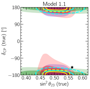
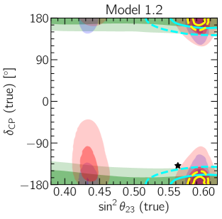
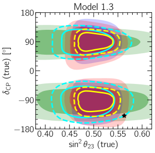
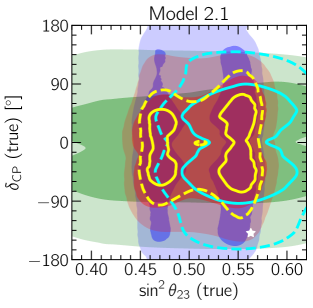
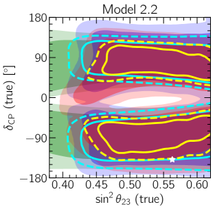
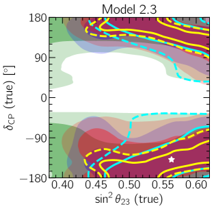
Figure 3.1: Compatibility of one and two-parameter models with any potentially true values of $\sin^{2}\theta_{23}$ and $\delta_{\rm CP}$ in the context of ESSnuSB,T2HK, DUNE, and their combination. The dark (light) green, blue, and red shaded regions represent $3\sigma$ (5$\sigma$) allowed regions for ESSnuSB, T2HK, DUNE respectively. Similarly, the continuous (doted) cyan and yellow lines represent 3$\sigma$ (5$\sigma$) allowed regions for ESSnuSB combined with atmospheric data and ESSnuSB long-baseline experiments. The stars are the best fit values. Figure taken from the arXiv version of  Ref. [418].

In Fig. 3.1, we show the compatibility of one and two-parameter models with any potentially true values of $\sin^{2}\theta_{23}$ and $\delta_{\rm CP}$ in the context of ESSnuSB, T2HK, DUNE, and their combination [418]. The models are based on $A_{5}\times CP$ (Model 1.1), $A_{5}\times CP$ (Model 1.2) $S_{4}\times CP$ (Model 1.3), $S_{4}\times CP$ (Model 1.4), $A_{5}\times CP$ (Model 1.5), $A_{5}$ (Model 2.1), $S_{4}$ (Model 2.2) and $A_{5}$ (Model 2.3) discrete groups. A detailed discussion on the specification of each model and their individual compatibility with a combination of experiments can be found in  Ref. [418]. In Fig. 3.1, the dark (light) green, blue, and red shaded regions represent $3\sigma$ (5$\sigma$) allowed regions for ESSnuSB, T2HK, DUNE respectively. Similarly, the continuous (doted) cyan and yellow lines represent 3$\sigma$ (5$\sigma$) allowed regions for ESSnuSB combined with atmospheric data and ESSnuSB long-baseline experiments. The complementarity among these neutrino oscillation experiments offers us some insight into distinguishing various classes of discrete flavor symmetric models. The best fit value for models 1.1, 1.2 falls outside experimentally allowed range of parameters whereas the model 2.3 satisfies all experimental constraints. As shown in Fig. 3.2, the high-precision measurement of $\sin^{2}\theta_{12}$ by JUNO will be crucial in discriminating among and excluding most of the considered models (see models 1.4 and 1.5 on left and models 1.1, 1.2, 1.4 on right of the $\sin^{2}\theta_{12}$ best-fit value.

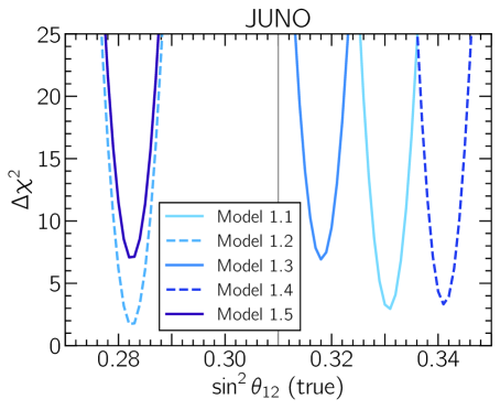
Figure 3.2: Compatibility of one-parameter models with any potentially true value of $\sin^{2}\theta_{12}$ in the context of JUNO. The vertical gray line indicates the best-fit value of $\sin^{2}\theta_{12}$ from global neutrino oscillation data discussed in  Ref. [418]. Figure taken from the arXiv version of  Ref. [418].

Leveraging DUNE’s excellent capability for $\delta_{\rm CP}$ and $\theta_{23}$ measurements, the prospects of generalized CP symmetries with texture zeros [426] and ‘bi-large’ mixing [427] have also been investigated. In another study [428], the authors have demonstrated an approach to construct operators for neutrino non-standard interactions based on $A_{4}$ discrete symmetry and its feasibility at DUNE. For studies of consequences of partial $\mu-\tau$ reflection symmetry at DUNE and Hyper-Kamiokande, see  Refs. [187, 429, 182]. Guided by the considered discrete flavor symmetry $G_{f}$, sum rules involving neutrino masses and mixing may also have inherent characteristics [430, 431, 286, 99] to be confronted with the neutrino experiments mentioned here. Usually, it is very hard to obtain specific correlations among the neutrino mixing parameters within the modular invariance approach and hence there are very few studies on the viability of these models in the context of neutrino oscillation experiments. Recently, in Ref. [432], the authors have discussed the implication of modular symmetry in neutrino oscillation experiments. In this work, three different $A_{4}$ modular symmetric models were considered. The numerical predictions of these three models were tested in the context of T2HK, DUNE, and JUNO experiments, showing a relative comparison of the models and their compatibility with these experiments. Furthermore, for a discussion on testing non-standard neutrino interactions at neutrino oscillation originating from modular invariance approach (as well as flavor symmetry-based approach), see Ref. [433].

3.2   Neutrinoless Double Beta Decay

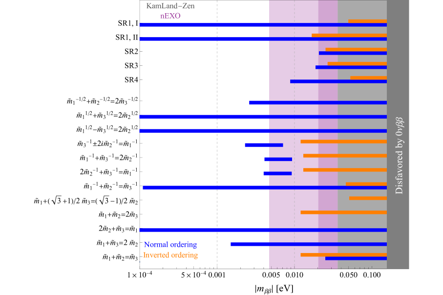
Figure 3.3: A summary plot of the predictions for $m_{\beta\beta}$ from different mass sum rules for NO and IO. The current experimental bound from KamLand-Zen Ref. [48] is shown in gray and the future sensitivity of nEXO Ref. [49] is in purple. The different shading corresponds to different values of the nuclear matrix elements, leading to the weakest and strongest bounds on $|m_{\beta\beta}|$. The figure is updated from Ref. [241].

Some flavor models based on discrete symmetries provide predictions for the absolute neutrino mass scale as well as the Majorana phases. Of particular interest are models that predict a correlation between the three complex neutrino mass eigenvalues and the Majorana phases, $\tilde{m_{i}}=m_{i}e^{i\alpha_{i}}$, hence allow only a certain portion of the parameter space shown in Fig. 1.2 for $0\nu\beta\beta$. This has been extensively studied in the literature in the context of different flavor models, e.g. TBM [233], $\mu-\tau$ [434], $A_{4}$ [435, 436], $S_{4}$ [249, 251, 437], $A_{4}\times Z_{4}$ [438], and $\Delta(3n^{2})$ [439]. A comprehensive summary of $0\nu\beta\beta$ predictions from five categories of flavor models, namely, generalized CP, sum rules, charged lepton corrections, texture zeros, and modular symmetries, can be found in Ref. [440]. As discussed in Ref. [241], neutrino mass sum rules are present in over sixty flavor models [236, 240, 430, 286, 285]. Fig. 3.3 (updated from Ref. [241]) gives a representation of the predictions for $m_{\beta\beta}$ from different mass sum rules, namely five sum rules connected with modular symmetry models (SR1-I, SR1-II, SR2, SR3, SR4) [285] and twelve sum rules connected with models that predict a correlation between the three complex neutrino mass eigenvalues [240]; see Section 2.3 for the explanation of the different sum rules. We can see clearly in Fig. 3.3 that the current KamLand-Zen constraint [48] has already killed some flavor models, and future experiments like nEXO [49] will be able to rule out the IO scenario for the remaining models, and also the NO scenario for some models.

3.3   Lepton Flavor and Universality Violation

Flavor symmetry models can also make distinctive predictions for LFV and LFUV observables. The basic idea is that couplings between flavons and leptons can result in special flavor structures with specific LFV predictions. Thus, discovering LFV signal can provide crucial information to distinguish flavor symmetries and new physics scenarios. See Refs. [441, 239] for reviews of the impact of flavor symmetry models on LFV processes. More recent studies of LFV in specific flavor models can be found in Refs. [442, 443, 444, 173, 445, 446]. For example, the FSS model [175] (reproducing TM₁ mixing with $A_{4}$ discrete flavor symmetry) described in Section 2.2 also contributes to LFV decays such as $\ell_{\alpha}\to\ell_{\beta}\gamma$ and $\ell_{\alpha}\to 3\ell_{\beta}$ ($\alpha,\beta=e,\mu,\tau$). Predictions of these LFV decays crucially depend on the VEV alignment of the associated flavons which also dictates the neutrino masses and mixing. Owing to the particular flavor structure given in Eqs. (2.54) and (2.55), the scotogenic part within this FSS framework only contributes to the LFV decay $\mu\to e\gamma$ and $\mu\to 3e$ conversion and puts a strong constraint on the allowed parameter space.

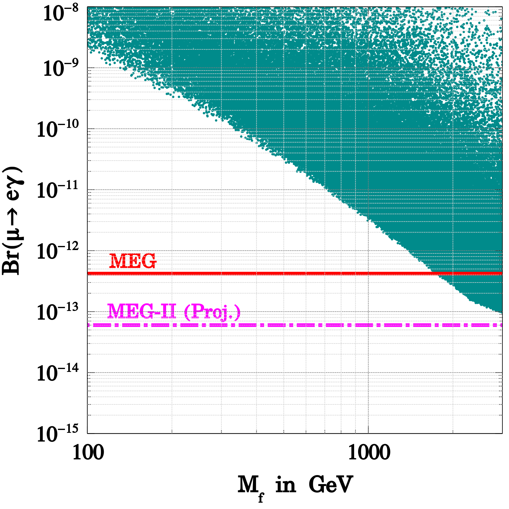
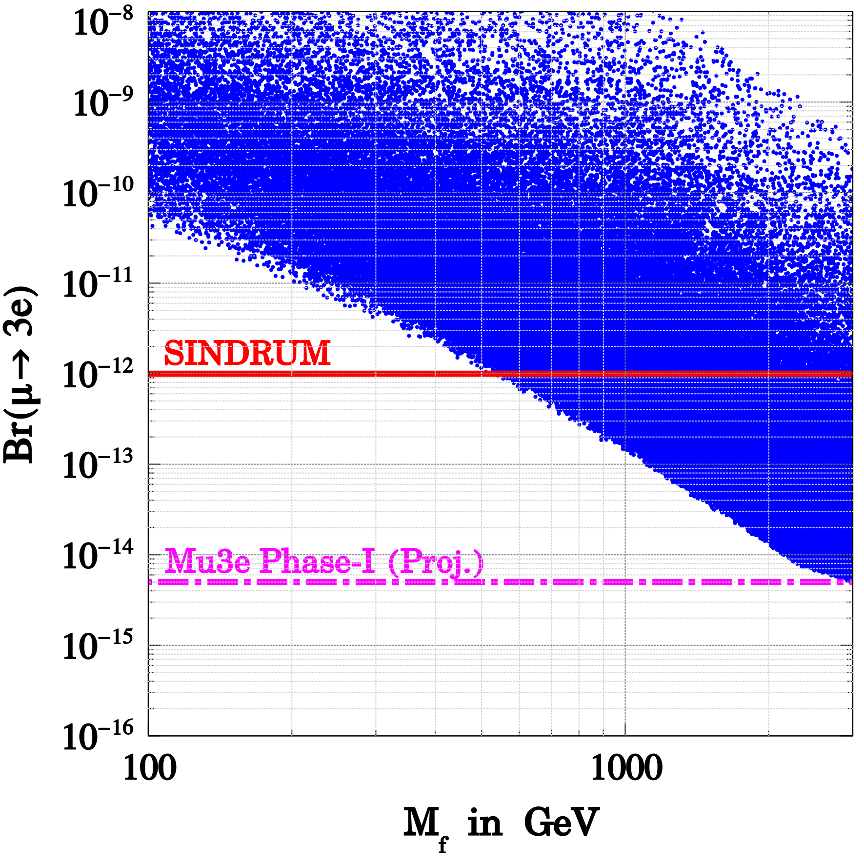
Figure 3.4: Branching ratios for $\mu\to e\gamma$ (left panel) and $\mu\to 3e$ (right panel) against scotogenic fermion mass $M_{f}$ satisfying $3\sigma$ allowed range of neutrino oscillation data [20] as well as correct DM relic density. The horizontal red and magenta lines represent current and future experimental sensitivity. Figure taken from Ref. [175].

In Fig. 3.4, we have shown the prediction for the branching ratios for $\mu\to e\gamma$ (cyan dots, left panel) and $\mu\to 3e$ (blue dots, right panel) against scotogenic fermion ($f$) mass $M_{f}$. In this FSS model, $f$ is also a potential DM candidate. In both panels of Fig. 3.4, the dotted regions represent the $3\sigma$ allowed regions which satisfy correct neutrino masses and mixing [20] as well as correct DM relic density. The horizontal red lines in both of these panels represent the current sensitivity of MEG [447] and SINDRUM [448] experiments and substantially contain the allowed parameter space and restrict DM mass $M_{f}\gtrsim$ 1750 GeV. More interestingly, this $A_{4}$ FSS model can be falsified by the future sensitivity (given by horizontal magenta line) of MEG II [449] and Mu3e Phase-I [450] experiment for $\mu\to e\gamma$ and $\mu\to 3e$ decays, respectively. On the other hand, due to the considered flavor symmetry, the Yukawa couplings $Y_{F}^{\tau}$, $Y_{N}^{e}$ vanish and hence $\tau\rightarrow 3e$ processes are strictly disallowed in this model. Thus, with an example of a $A_{4}$ flavor symmetric scoto-seesaw framework, we find that flavor symmetry can have distinct consequences on lepton flavor violating decays.

In some cases, the flavor model predictions for LFV, especially in the tau sector, are expected to be probed in the near future by Belle II. The role of leptonic CP phases (which come out as a prediction in many flavor models) in the LFV observables has been explored recently in Ref. [451]. Now, considering the mixing of light and heavy RHNs, flavor symmetric models can also constrain the VEV of the flavon fields involved, which helps to realize the desired flavor structure to explain observed leptonic mixing. Following Eqs. (1.19)-(1.22), the leptonic non-unitarity can be defined as [452, 453, 454, 455]

$$U\simeq(\mathbb{I}-\eta)U_{\rm PMNS}$$ (3.1)

where the non-unitary parameter is defined as $\eta=\frac{1}{2}FF^{\dagger}$ and $F=M_{D}M_{R}^{-1}$. The present bound on $\eta$ obtained from various non-standard interactions can be summarized as [453, 455, 456]

$$|\eta|\leq\left(\begin{array}[]{ccc}1.3\times 10^{-3}&1.2\times 10^{-5}&1.4\times 10^{-3}\\ 1.2\times 10^{-5}&2.2\times 10^{-4}&6.0\times 10^{-4}\\ 1.4\times 10^{-3}&6.0\times 10^{-4}&2.8\times 10^{-3}\end{array}\right).$$ (3.5)

In a flavor symmetric model, the mass matrices for the Dirac ($M_{D}$) and heavy Majorana ($M_{R}$) neutrinos appearing in $\eta$ can be obtained with the involvement of the flavons. Hence, the constraints on $\eta$ for Eq. (3.5) can, in principle, constrain the VEV of the associated flavon field. For example, considering an $A_{4}$ flavor symmetric inverse seesaw scenario in Ref. [157], the authors showed that the flavon VEV ($v_{f}$) can be constrained as $v_{f}\leq 6.15{\lambda}$ TeV, where $\lambda$ is the ratio of the modulus of the coupling constants involved in $M_{D}$ and $M_{R}$ respectively. Along with the constrain on $\eta$ given in Eq. (3.5), the Dirac CP phase $\delta_{\rm CP}$ can also play an instrumental role in obtaining limits on $v_{f}$; for a detailed discussion see Ref. [157].

Flavor models can also shed some light on the recent hints for lepton flavor universality violation. In Ref. [457], a comprehensive analysis is given based on the flavor group $G_{f}=D_{17}\times Z_{17}$ with scalar leptoquarks aiming to explain some anomalies in $B$-physics connected with lepton flavor universality between $\tau$ and $e,\mu$, as well as muon anomalous magnetic moment $g-2$. For other studies of the LFUV in flavor symmetry models, see e.g. Refs. [458, 459, 460].

4   Flavor Symmetry at Energy Frontier

Flavor models with extended particle content can lead to interesting collider signals. For instance, in the flavor models with Majorana RHNs, the structure of the complex Dirac Yukawa couplings can be fixed by the flavor (and CP) symmetries. This in turn gives concrete predictions for the LNV/LFV signatures associated with the RHNs, depending on their mass spectrum. In this section, we will illustrate the collider phenomenology in a class of models with residual flavor and CP symmetries. The specific discrete flavor symmetry groups $G_{f}$ chosen here are the series of groups $\Delta(6\,n^{2})$ [461], known to give several interesting neutrino mixing patterns [355, 356, 462, 360, 439]. As discussed in Refs. [463, 464], this framework provides an excellent probe of flavor symmetries in collider experiments. For example, it can result in one of the three RHNs to be very long-lived at some special parameter points, termed as points of enhanced residual symmetry (ERS), which can be searched through long-lived particle (LLP) searches [465, 466]. In comparison, the remaining two RHNs can be probed via prompt/displaced vertex signals at the LHC [467, 468] or future hadron collider FCC-hh [469, 470]; see discussion in Section 4.2.

4.1   Example Group : $\Delta(6n^{2})$

The discrete groups $\Delta(6\,n^{2})$, ($n\in Z,\,n\geq 2$)  [461], can be characterized by four generators $a$, $b$, $c$ and $d$ along with the identity element $e$, fulfilling the relations

$$a^{3}\,=\,e\;,\;\;c^{n}\,=\,e\;,\;\;d^{n}\,=\,e\;,\;\;c\,d\,=\,d\,c\;,\;\;a\,c\,a^{-1}\,=\,c^{-1}d^{-1}\;,\;\;a\,d\,a^{-1}\,=\,c\,,$$

$$b^{2}\,=\,e\;,\;\;(a\,b)^{2}\,=\,e\;,\;\;b\,c\,b^{-1}\,=\,d^{-1}\;,\;\;b\,d\,b^{-1}\,=\,c^{-1}\,.$$ (4.1)

Upon breaking of the the flavor group $G_{f}$ at low energies, the neutrino and charged lepton sectors are still invariant under residual flavor and CP symmetry groups. The residual symmetry in the charged lepton sector is chosen to be the diagonal abelian subgroup of $Z_{3}$, i.e. $G_{\ell}=Z_{3}^{(\mathrm{D})}$, while in the neutrino sector, we choose the residual symmetry to be $G_{\nu}=Z_{2}\times{\rm CP}$. The generators of $Z_{2}$ symmetry $Z(\mathrm{r})$ and CP symmetry $X(\mathrm{r})$ commute for all representations ${\rm r}$ of $G_{f}$. The transformations related to CP symmetry correspond to the automorphisms of the flavor group. The differences between the residual symmetries $G_{\ell}$ and $G_{\nu}$ determine the forms of the lepton mixing matrix, charged lepton mass matrix, the neutrino Yukawa $Y_{D}$ and the RHN Majorana mass matrix $M_{R}$. Since, we explicitly choose the charged lepton mass matrix to be diagonal, the charged lepton sector does not contribute to the lepton mixing. As for the neutrino sector, we assume the Dirac neutrino Yukawa coupling matrix $Y_{D}$ to be invariant under $G_{\nu}$ and the Majorana matrix $M_{R}$ does not break either $G_{f}$ or CP. The light neutrino masses are obtained by the type-I seesaw formula [195, 196]:

$$M_{\nu}=-v^{2}Y_{D}M_{R}^{-1}Y_{D}^{T}\,,$$ (4.2)

where $v$ is the SM Higgs VEV.

As an example, we consider a particular case with generator of $Z_{2}$ symmetry $Z\,=\,c^{n/2}$, where $c$ is one of the generators of the group $\Delta(6n^{2})$ and the corresponding CP transformations reads $X(s)=\ a\,b\,c^{s}\,d^{2s}\,P_{23}$, where $s$ is a parameter that runs from $0$ to $(n-1)$ and $P_{23}$ is the permutation matrix in the 2-3 plane. For this case, the form of $Y_{D}$ is given by

$$Y_{D}\,=\,\Omega^{s}({3})\,R_{13}(\theta_{L})\,\left(\begin{array}[]{ccc}y_{1}&0&0\\ 0&y_{2}&0\\ 0&0&y_{3}\end{array}\right)\,R_{13}(-\theta_{R})\,\Omega^{s}({3^{\prime}})^{\dagger}\;,$$ (4.3)

where the angles $\theta_{L}$ and $\theta_{R}$ are free parameters, with values in the range $[0,\pi)$ and $R_{ij}(\theta)$ denotes rotation by an angle $\theta$ in the $ij$ plane. $\Omega^{s}({3})$ is a unitary matrix connected with $X({3})(s)$, with the following structure:

$$\Omega^{s}({3})\,=\,e^{i\phi_{s}}\,U_{\mathrm{TBM}}\,\left(\begin{array}[]{ccc}1&0&0\\ 0&e^{-3\phi_{s}}&0\\ 0&0&-1\end{array}\right)\,$$ (4.4)

(where $\phi_{s}=\pi s/n$), whereas the form of the unitary matrix $\Omega^{s}({3^{\prime}})$ depends on whether $s$ is even or odd, i. e.

$$\Omega^{s\;\rm{even}}({3^{\prime}})\,=\,U_{\mathrm{TBM}}\;,\>\>\Omega^{s\;{\rm odd}}({3^{\prime}})\,=\,U_{\mathrm{TBM}}\,\left(\begin{array}[]{ccc}i&0&0\\ 0&1&0\\ 0&0&i\end{array}\right)\;,$$ (4.8)

with $U_{\rm TBM}$ given in Eq. (1.18). Finally, we can find the form for the PMNS mixing matrix as

$$U\,=\,\Omega^{s}({3})\,R_{13}{(\theta_{\rm L}-\psi)}\,K_{\nu}\,,$$ (4.9)

where $K_{\nu}$ is a diagonal matrix with entries equal to $\pm 1$ and $\pm{i}$, making neutrino masses non-negative, and the angle $\psi$ is defined by

$$\tan^{2}\psi=\frac{m_{1}+m_{3}-\sqrt{m_{1}^{2}+m_{3}^{2}+2m_{1}m_{3}\cos(4\theta_{R})}}{m_{1}+m_{3}+\sqrt{m_{1}^{2}+m_{3}^{2}+2m_{1}m_{3}\cos(4\theta_{R})}}\,.$$ (4.10)

$\theta_{L}$ in Eq. (4.9) is determined by reproducing the best-fit values of the measured neutrino mixing angles (cf. Tab. 1.1).

As for the RHN Majorana mass matrix $M_{R}$, since it leaves $G_{f}$ and CP invariant, its form is s imply

$$M_{R}\,=\,M_{N}\,\left(\begin{array}[]{ccc}1&0&0\\ 0&0&1\\ 0&1&0\end{array}\right)\,,$$ (4.11)

with $M_{N}>0$ setting the overall mass scale of the RHNs. From Eq. (4.11), we see that the three RHNs are exactly degenerate in the flavor symmetry limit. However, if we want to successfully generate the BAU via resonant leptogenesis [471, 472] using the RHN freeze-out in the early universe, we need at least two quasi-degenerate RHNs. This can be achieved by introducing a small symmetry breaking term (that can be sourced from higher-dimensional operators)

$$\delta M_{R}=\kappa\,M_{N}\,\left(\begin{array}[]{ccc}2&0&0\\ 0&0&-1\\ 0&-1&0\end{array}\right)$$ (4.12)

with $\kappa\ll 1$. Then the RHN masses acquire a (small) correction

$$M_{1}=M_{N}\,(1+2\,\kappa)\;\;\mbox{and}\;\;M_{2}=M_{3}=M_{N}\,(1-\kappa)\,,$$ (4.13)

thus making two RHN pairs quasi-degenerate, adequate for resonant leptogenesis (see Section 4.4).

Above we sketched a typical construction connected with CP and discrete flavor symmetries in the lepton sector, leading to the parametrization of the Dirac Yukawa coupling matrix given by Eq. (4.3). This is a very predictive scenario, with only five real parameters determining the lepton mixing, namely, three Yukawa couplings $(y_{1},y_{2},y_{3})$ corresponding to the three light neutrino masses, and two rotation angles ($\theta_{L}$ and $\theta_{R}$) for lepton mixing. Just two extra parameters ($\kappa$ and $M_{N}$) are needed for explaining the BAU. For TeV-scale $M_{N}$, this leads to interesting predictions that can be tested at both energy and intensity frontier experiments. In the following, we will briefly discuss some phenomenological features of this simple scenario. For more details, see Ref. [464].

4.2   Decay Lengths and Branching Ratios of RHNs

TeV-scale Majorana RHNs give rise to spectacular multilepton signals at the LHC and future colliders [467, 468, 473, 474]. The general problem is to get substantial production rate. In the context of minimal type-I seesaw for our TeV-scale RHN scenario, light neutrino masses and mixing require the Yukawa couplings to be significantly suppressed, with values on the order of $10^{-7}$. This, in turn, suppresses the Drell-Yan production of the RHNs at LHC for the smoking-gun signal of same-sign dilepton plus two jets without missing transverse energy [475, 476, 477, 478, 479, 480, 481, 482, 483, 484, 485, 486]. However, in typical UV-complete RHN models with additional gauge interactions, the production rate can be enhanced without relying on their mixing with the SM neutrinos [467]. For example, in $U(1)_{B-L}$ extensions of the SM [487, 488], the RHNs can be pair-produced via the $Z^{\prime}$-mediated process: $pp\to Z^{\prime}\to NN$ [489, 490, 491, 492, 493, 494, 495, 496]. Similarly, in the left-right symmetric models based on the $SU(2)_{L}\times SU(2)_{R}\times U(1)_{B-L}$ gauge group [364, 497, 498], the RHNs can be produced via the RH current: $pp\to W_{R}\to N\ell$ [475, 499, 500, 501, 502, 503, 504, 505, 506, 507, 508, 509, 510, 511]. Depending on the new gauge boson mass, cross sections up to a few fb are possible at the LHC.

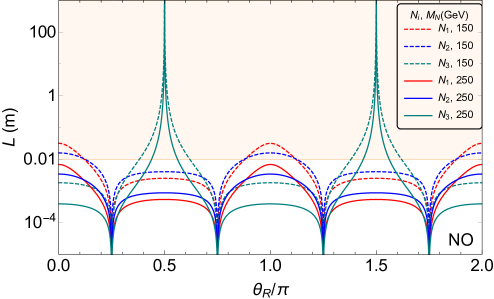
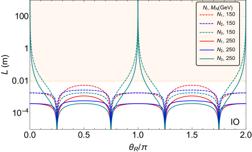
Figure 4.1: Decay lengths for $N_{1,2,3}$ are plotted against $\theta_{R}$ for different values of the RHN mass scale $M_{N}$ (with $m_{0}=0$). The left (right) panel is for NO (IO). The shaded (unshaded) region roughly indicates the displaced/long-lived (prompt) signal regime. Figure adapted from Ref. [464] under CC BY 4.0 license.

After being produced, the RHNs typically decay into SM final states: $N\to W\ell,\,Z\nu,\,h\nu$ [479]. The total decay width $\Gamma_{i}$ of the RHN $N_{i}$ at the tree-level depends on the Yukawa coupling $Y_{D}$, and is given by

$$\Gamma_{i}\,=\,\frac{(Y_{D}^{\dagger}\,Y_{D})_{ii}}{8\,\pi}M_{i}.$$ (4.14)

Thus in flavor symmetry models, the RHN decay lengths depend indirectly on the choice of the generator $Z(\mathbf{r})$ of the $Z_{2}$ symmetry and the choice of the CP transformation $X(\mathbf{r})$. For the example case considered above, see Eq. (4.3), the expressions for the decay widths are independent of values of $s$ and only depend on the Yukawa couplings $y_{f}$ and the angle $\theta_{R}$:

$$\Gamma_{1}\, =\,\frac{M_{N}}{24\,\pi}\,\left(2\,y_{1}^{2}\,\cos^{2}\theta_{R}+y_{2}^{2}+2\,y_{3}^{2}\,\sin^{2}\theta_{R}\right)\,,$$ (4.15a)

$$\Gamma_{2}\, =\,\frac{M_{N}}{24\,\pi}\,\left(y_{1}^{2}\,\cos^{2}\theta_{R}+2\,y_{2}^{2}+y_{3}^{2}\,\sin^{2}\theta_{R}\right)\,,$$ (4.15b)

$$\Gamma_{3}\ =\,\frac{M_{N}}{8\,\pi}\,\left(y_{1}^{2}\,\sin^{2}\theta_{R}+y_{3}^{2}\,\cos^{2}\theta_{R}\right)\,.$$ (4.15c)

We can convert these decay rates into decay lengths $L_{i}=\gamma/\Gamma_{i}$ in the laboratory frame, where $\gamma$ is the boost factor of RHN which can be determined depending on how the RHN is produced. Some numerical results for the decay lengths based on Eqs. (4.15) are plotted in Fig. 4.1 as a function of $\theta_{R}$. Here we have assumed the production of RHNs via $Z^{\prime}$ with mass $M_{Z^{\prime}}=4$ TeV in a $U(1)_{B-L}$ model, which implies $\gamma=M_{Z^{\prime}}/2M_{N}=8~{}(13.3)$ for $M_{N}=250~{}(150)$ GeV. We find that the decay lengths are connected with neutrino mass ordering, as strong NO arises for $y_{1}=0$ so that $m_{1}$ vanishes, $m_{2}=y_{2}^{2}\,v^{2}/M_{N}$ and $m_{3}=y_{3}^{2}\,|\cos 2\,\theta_{R}|\,v^{2}/M$, while strong IO arises for $y_{3}=0$ so that $m_{3}=0$, $m_{1}=y_{1}^{2}\,|\cos 2\,\theta_{R}|\,v^{2}/M_{N}$ and $m_{2}=y_{2}^{2}\,v^{2}/M_{N}$. As can be seen from the decay length expressions (4.15), for strong NO and strong IO corresponding to $y_{1}=0$ and $y_{3}=0$ respectively (i.e. when $m_{0}=0$), there are ERS points for $\theta_{R}\to\pi/2,\,3\pi/2$ (NO) or $\theta_{R}\to 0,\,\pi$ (IO), at which $\Gamma_{3}\to 0$, i.e. the RHN $N_{3}$ becomes long-lived. The larger the ERS is, the smaller the deviation from points of ERS will be, i.e. $\theta_{R}$ is expected to deviate from $\theta_{R,0}$ by a small amount, $\delta\theta_{R}=|\theta_{R}-\theta_{R,0}|$. For $10^{-4}\lesssim\delta\theta_{R}\lesssim 10^{-2}$, this could lead to displaced vertex signatures from $N_{3}$ decay that are accessible to future dedicated LLP experiments, such as FASER [512] and MATHUSLA [463]. Most signals from $N_{1,2}$ decays are prompt but can also be slightly displaced depending on the choice of $\theta_{R}$. The distinction between the two cases (prompt vs displaced) is marked here by $L=1$ cm (horizontal line in Fig. 4.1) for the LHC, although the exact value might vary slightly depending on the details of the detector (CMS vs ATLAS). The points of ERS are of particular relevance for phenomenology since $\theta_{L}$ deviating from $\theta_{L,0}=$ $0$ or $\pi$ leads to a non-zero value of the reactor mixing angle $\theta_{13}$. ERS points are also relevant for leptogenesis, as discussed in Chapter 5.

The underlying Yukawa structure $Y_{D}$ not only predicts the decay lengths of the RHNs, but also their decay branching ratios (BRs), as the partial decay widths are proportional to $\left|\left(Y_{D}\right)_{\alpha i}\right|^{2}$. Considering the decay of long-lived $N_{3}$ at an LLP detector with $m_{0}=0$ and $M_{N}=250$ GeV, we find the following proportion of BRs:

$${\rm BR}(N_{3}\to e^{\pm}W^{\mp}):{\rm BR}(N_{3}\to\mu^{\pm}W^{\mp}):{\rm BR}(N_{3}\to\tau^{\pm}W^{\mp})\,=\,\left\{\begin{array}[]{ll}1:27.7:18.1&({\rm NO})\\ 8.5:1:3.7&({\rm IO})\end{array}\right.,$$ (4.16)

independent of $\theta_{R}$ and $s$, and almost independent of $M_{N}$, if $M_{N}\gg m_{W}$. Thus, measuring these RHN decay BRs at an LLP detector for at least two charged lepton flavors provides an independent test of the neutrino mass hierarchy at the energy frontier. Decay signals of $N_{1,2}$ at LHC (prompt or displaced vertex) can also be used to test mass hierarchy, but specifically, they depend on $\theta_{R}$ as well as on the chosen CP symmetry $X(s)$.

4.3   Lepton Flavor Violation at Colliders

The decays of Majorana RHNs into charged leptons lead to LNV as well as LFV signals. Consider the $Z^{\prime}$-mediated production that leads to the same-sign dilepton final state [492]:

$$pp\to Z^{\prime}\to N_{i}N_{i}\to\ell_{\alpha}^{\pm}\ell_{\beta}^{\pm}+2W^{\mp}\to\ell_{\alpha}^{\pm}\ell_{\beta}^{\pm}+4j\,.$$ (4.17)

Since the partial decay widths of RHNs depend on $Y_{D}$, the LNV signal cross-section is affected by the choice for generator $Z$ of the $Z_{2}$ symmetry and the choice of the CP transformation $X$, see discussion in Section 4.1.

We can probe the high-energy CP phases in the Yukawa coupling matrix at colliders by constructing simple observables out of the same-sign dilepton charge asymmetry. In particular, we can define two observables $\sigma_{\rm LNV}^{\alpha,-}$ (difference) and $\sigma_{\rm LNV}^{\alpha,+}$ (sum) of the same-sign charged-lepton final states of a given flavor $\alpha$:

$$\sigma_{\rm LNV}^{\alpha,\pm}\,=\, \sum_{i}\sigma_{\rm prod}(pp\to N_{i}N_{i})\left(\left[{\rm BR}(N_{i}\to\ell_{\alpha}^{-}W^{+})\right]^{2}\pm\left[{\rm BR}(N_{i}\to\ell_{\alpha}^{+}W^{-})\right]^{2}\right)\times\left[{\rm BR}(W\to jj)\right]^{2}\,.$$ (4.18)

The flavored CP asymmetries $\varepsilon_{i\alpha}$ relevant for leptogenesis turn out to be related to the ratio $\sigma_{\rm LNV}^{\alpha,-}/\sigma_{\rm LNV}^{\alpha,+}$ [513, 514, 515]. Thus, measuring $\sigma_{\rm LNV}^{\alpha,-}/\sigma_{\rm LNV}^{\alpha,+}$ can help measure the CP asymmetry, which is predicted by the group theory parameters. The normalized LNV cross sections $\sigma_{\rm LNV}(\ell^{\pm}_{\alpha}\ell^{\pm}_{\beta})$ with respect to the new gauge coupling $g^{\prime}$ for our example case are shown in Fig. 4.2. It can be concluded that comparing the LNV final states with different charged-lepton flavor combinations can provide an independent, complementary test of the neutrino mass ordering at the high-energy frontier.

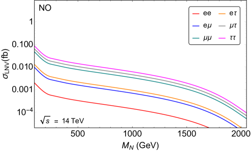
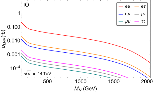
Figure 4.2: Normalized LNV signals as a function of the RHN mass scale $M_{N}$ at $\sqrt{s}=14$ TeV LHC for all possible lepton flavor combinations in the strong NO (left) and strong IO (right) limit. Here we have fixed $M_{Z^{\prime}}=4$ TeV. Figure taken from the arXiv version of Ref. [464].

4.4   Correlation between Collider Signals and Leptogenesis

Leptogenesis [516] provides an attractive link between two seemingly distinct hints for BSM physics, namely, neutrino masses and mixing, and the observed BAU, via the seesaw mechanism [196]. General details of the leptogenesis mechanism will be discussed in Section 5.2. Here, we briefly summarize the collider prospects of testing TeV-scale resonant leptogenesis [471] in the $\Delta(6n^{2})$ flavor model discussed in Section 4.1, along with an extra $U(1)_{B-L}$ so that TeV-scale RHNs can be produced more efficiently at colliders than in the minimal type-I seesaw. In principle, we could also consider other gauge groups under which the RHNs and the SM are charged, such as the left-right symmetric framework. However, it turns out that in the left-right models, the additional washout effects induced by the right-handed gauge interactions impose a lower bound of $M_{W_{R}}\gtrsim 20$ TeV to get successful leptogenesis, thereby precluding the possibility of testing it at the LHC [517, 518, 510, 519]. On the other hand, the corresponding leptogenesis bound in the $U(1)_{B-L}$ model considered here is rather weak due to the double Boltzmann suppression of the $Z^{\prime}$-induced washout effects [514, 520, 521].

In the presence of the RHNs, the flavored CP symmetries $\varepsilon_{i\alpha}$ for resonant leptogenesis depend on the structure of $Y_{D}$ (see Section 5.2), and therefore, can be computed analytically using the form of $Y_{D}$ given in Eq. (4.3) for the flavor model considered here. This CP asymmetry can then be translated into a BAU ($\eta_{B}$) as described in Section 5.2, and compared with the observed value $\eta_{B}^{\rm obs}$. Since the CP asymmetry is a function of $Y_{D}$, the choice for generator $Z$ of the $Z_{2}$ symmetry and the choice of the CP transformation $X$ determines the form of $\varepsilon_{i}$ and in turn, the $\eta_{B}$.

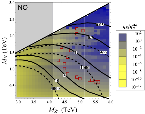
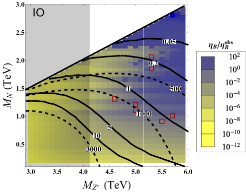
Figure 4.3: Prediction for BAU $\eta_{B}$ relative to the observed value $\eta_{B}^{\rm obs}$ in the $(M_{Z^{\prime}},M_{N})$ plane for a fixed $g_{B-L}=0.1$ in a $\Delta(6n^{2})$ model for strong NO (IO) in the left (right) panel, with $\theta_{R}$ set to the respective ERS points. The red boxes correspond to $\eta_{B}$ within $10\%$ of $\eta_{B}^{\rm obs}$. The contours show the RHN production cross sections (in ab) at the $\sqrt{s}=14$ TeV LHC (solid) and at $\sqrt{s}=100$ TeV FCC-hh (dashed). The vertical shaded region is the current exclusion from LHC dilepton data. Figure taken from Ref. [464].

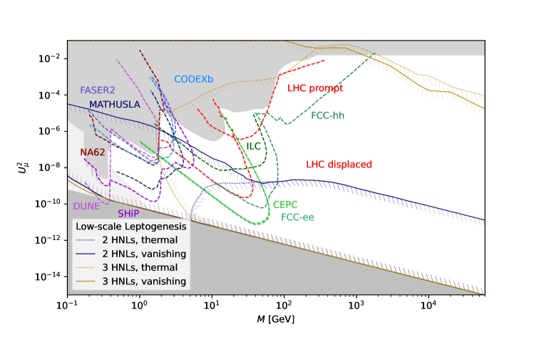
Figure 4.4: Summary of LHC and future collider sensitivities to different low-scale leptogenesis scenarios with two and three RHNs. The upper (lower) shaded regions are excluded by laboratory (seesaw) constraints. In the legend, HNLs means ‘Heavy Neutral Leptons’, which are called RHNs in this review. The $x$-axis is the RHN mass scale, and the $y$-axis gives the square of the light-heavy neutrino mixing in the muon flavor, which has the best experimental prospects (compared to electron and tau flavors). Figure taken from the arXiv version of Ref. [522] .

Fig. 4.3 shows the predictions for $\eta_{B}/\eta_{B}^{\rm obs}$ in the $(M_{Z^{\prime}},M_{N})$ plane for both NO (left) and IO (right) in a particular case of the $\Delta(6n^{2})$ model at ERS points [464]. The red boxes correspond to $\eta_{B}$ within $10\%$ of $\eta_{B}^{\rm obs}$. Now to see whether these points are accessible at colliders, we superimpose the RHN pair-production cross sections $\sigma(pp\to Z^{\prime}\to N_{i}N_{i})$ in attobarns (ab) for both $\sqrt{s}=14$ TeV LHC (solid contours) and $\sqrt{s}=100$ TeV FCC-hh (dashed contours). Successful leptogenesis for strong NO yields $\sigma_{\mathrm{prod}}\lesssim 5$ ab at $\sqrt{s}=14$ TeV LHC, which makes it difficult to get any observable events even with the final target luminosity of 3 ab^-1 at HL-LHC. The situation worsens for strong IO, where the cross sections are smaller by at least an order of magnitude compared to the strong NO case. On the other hand, a future $100$ TeV hadron collider like FCC-hh [470] can reach a $\sigma_{\mathrm{prod}}$ up to $2000$ ab for the region of successful leptogenesis, which should yield up to 1000 LNV events with 30 ab^-1 integrated luminosity. In fact, by going to higher $Z^{\prime}$ masses, the detection prospects at 100 TeV collider can be improved significantly. This is due to relaxed experimental limits on the new gauge coupling $g_{B-L}$ for $M_{Z^{\prime}}\gtrsim 6$ TeV [523]. For instance, at $M_{Z^{\prime}}=7$ TeV, $g_{B-L}$ can be as large as one. Since $\sigma_{\mathrm{prod}}$ scales as $g_{B-L}^{2}$ for $M_{N}<M_{Z^{\prime}}/2$, apart from a mild suppression due to change in the $Z^{\prime}$ mass, the cross-section gets enhanced by a factor of 100. The detection prospects will be even better in other $Z^{\prime}$ model variants like the leptophobic case, where the LHC bound is somewhat weaker.

In general, not working within the context of any particular flavor model, the current status and future prospects of testing low-scale leptogenesis in colliders and other laboratory experiments are summarized in Fig. 4.4 for the minimal type-I seesaw with either two or three RHNs [522]. It illustrates the fact that LHC and future colliders provide ample opportunity to test low-scale leptogenesis parameter space. One can also note a large enhancement in the allowed mixing-mass space for three RHNs compared to the two RHN scenario. The exact picture depends strongly on the leptogenesis scenarios with degenerate or non-degenerate RHNs, freeze-in and freeze-out transitions, thermal initial conditions, LFV and oscillation constraints (e.g. mass of the lightest neutrino $m_{0}$). For an update, see also the talk in Ref. [524]. For other works showing the collider/laboratory prospects of testing low-scale leptogenesis, see Refs. [525, 526, 527, 528]. Phenomenological aspects of the high- and low-scale leptogenesis with RHNs in the context of BAU and discrete symmetries will be further discussed in Chapter 5.

4.5   Collider Signals in Other Flavor Models

In the above discussions involving the group $\Delta(6n^{2})$ discussed in Section 4.1, it is clear that the analyses of the flavor symmetry models lead to the rich phenomenology connected with intensity and energy frontiers. Such phenomenological studies of discrete flavor symmetries can be extended to other discrete groups as well. We discuss below a few of these possibilities.

In Ref. [529], a model has been considered with two Higgs doublets and flavor symmetry $A_{4}\times{Z}_{2}\times{Z}^{\prime}_{2}$, which can explain large leptonic mixing angles through a specific alignment of VEVs in the scalar sector. In Ref. [530], some phenomenological consequences of the model for collider physics and the DM problem were further explored. The $Z_{2}$-even scalar fields of the considered model give two generations of fields that couple completely off-diagonally to the charged leptons. Thus, the model predicts LFV processes $\tau\to\mu\mu e$, $\mu\to e\gamma$ and $e^{+}e^{-}\to\tau^{+}\mu^{-}$. As a consequence, LFV processes can also be searched for at hadron colliders (with an expectation of about ten events in each case) through the process $pp\to jjH_{2}H_{2}\to 2j4\ell$, where $H_{2}$ denotes either of the neutral components of the second generation $Z_{2}$-even scalar field. There are also contributions to the diphoton decay width of the Higgs boson. Still, even with couplings to the charged scalars of order unity, the deviations from the SM prediction are beyond the reach of HL-LHC. However, these percent level deviations from SM for scalar masses around TeV could be studied with future lepton colliders. The non-standard sector of this model is rich enough to include DM candidates (scalars and Majorana neutrinos). As shown in the analysis, they can also be probed at hadron colliders, with the possibility to account for the observed relic density for DM with a mass between 47 and 74 GeV or in the interval 600 GeV and 3.6 TeV.

A comprehensive collider study of the parameter space of the flavor symmetry group $A_{4}$ was performed in Ref. [531]. At the leading order, breaking the flavor group into residual symmetries $Z_{3}$($Z_{2}$) in the charged lepton (neutrino) sector generates the TBM mixing. The required fit to the observed PMNS matrix is achieved through slightly broken residual symmetries induced by a shift in one of the flavon VEVs. A thorough study in constraining the 6-dimensional model parameter space is conducted using the experimental data from $g-2$, MEG, Higgs scalar mixing, Higgs width measurements, and a recast $8$ TeV ATLAS analysis. The most stringent results are obtained from the LFV limit on ${\rm BR}(\mu\to e\gamma)$ set by the MEG experiment, leading to approximately $60\%$ parameter space to be excluded and the recast ATLAS analysis leading to $40\%$ exclusion.

In another work [532], the authors consider studies on LFV Higgs decays in the context of 3HDM with $S_{4}$ symmetry. A remnant $Z_{3}$ symmetry, which arises due to a specific vacuum alignment, leads to strongly suppressed FCNC. However, this symmetry is slightly broken by perturbations, leading to mixing between the scalars and, hence, to LFV Higgs decays. The original motivation for this work was to explain the $2.4\sigma$ anomaly in $h\rightarrow\mu\tau$ channel reported by CMS in 2015. They find if the extra scalars are light, the contribution to $\ell^{\prime}\rightarrow\ell\gamma$ can be suppressed while the flavor-violating couplings are still allowed to be large. Due to the $S_{4}$ symmetry, sizable $h\rightarrow\mu\tau$ leads to enhanced branching fractions also for LFV decays $h\rightarrow e\mu\,,e\tau$. Another study correlating the LFV Higgs and $Z$-boson decays to LFV in the charged lepton sector can be found in Ref. [533].

In Ref. [534], collider signatures of $T_{7}$ flavor symmetry with gauged $U(1)_{B-L}$ are studied for a renormalizable two-parameter neutrino model. So a mixture of discrete and continuous symmetries is also possible. Specifically, prospects for $Z^{\prime}$ production and detection at LHC through decays into neutral Higgs scalars are studied, which subsequently decay into charged leptons with a specific flavor pattern determined from the flavor symmetry group.

As another example, collider signatures of vector-like fermions (VLF) with a non-abelian flavor symmetry group $Q_{6}\times Z_{2}$ symmetry is studied in Ref. [535]. This group determines fermion masses as well as mixing. Only the third-generation fermions get their masses directly, while the rest obtain their masses in a see-saw-like mechanism. In this work, genetic algorithms are used to optimize the construction of neural networks that can maximize the statistical significance of a possible discovery (if any) for these VLFs at HL-LHC. While vector-like leptons can only probe masses safely up to $200$ GeV, the prospects for vector-like quarks are better with sensitivity up to $3.8$ TeV.

In a unified supersymmetric framework based on GUT $SU(5)\times A_{4}$ symmetry [376], studies on muon anomalous magnetic moment $g-2$ and DM have been performed in the context of LHC data where the right-handed smuon with masses are predicted to be around 100 GeV and with lightest (non-universal) gaugino masses being around 250 GeV.

4.6   Higgs to Diphoton Decay

The LHC data on the diphoton decay channel of the SM Higgs boson (with mass 125 GeV) [536, 537] can also have interesting phenomenological consequences in the context of discrete flavor symmetric scenarios. For example, for the scoto-seesaw FSS TM₂ model discussed in Section 2.2, the partial width of $h\to\gamma\gamma$ receives additional and significant contributions due to the $\eta^{\pm}$ and $\eta_{R}$ one-loop effects [175]. The signal strength of $h\rightarrow\gamma\gamma$ relative to the SM prediction is given by

$$R_{\gamma\gamma} = \frac{\big{[}\sigma(gg\to h)\times{\rm Br}(h\to\gamma\gamma)\big{]}_{\rm Model}}{\big{[}\sigma(gg\to h)\times{\rm Br}(h\to\gamma\gamma)\big{]}_{\rm SM}}=\frac{\Gamma^{\rm SM}_{\rm Total}\times\Gamma(h\to\gamma\gamma)_{\rm Model}}{\Gamma^{\rm Model}_{\rm Total}\times\Gamma(h\to\gamma\gamma)_{\rm SM}}.$$ (4.19)

While computing $R_{\gamma\gamma}$ in our analysis, we have taken the total decay width of the Higgs boson in the SM as $\Gamma_{\rm Total}^{\rm SM}=4.1$ MeV [538].

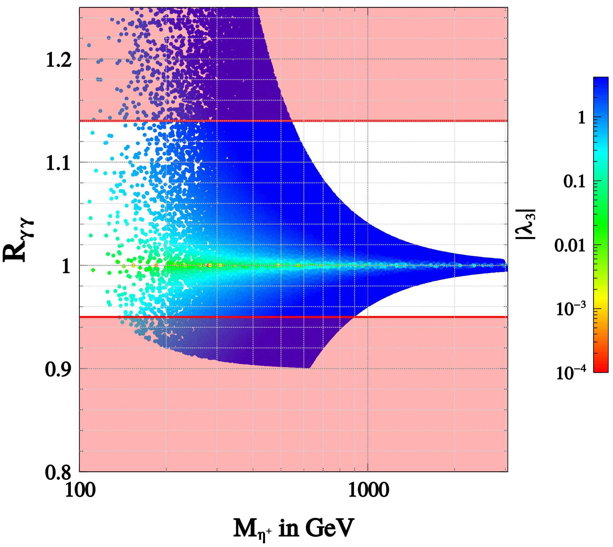
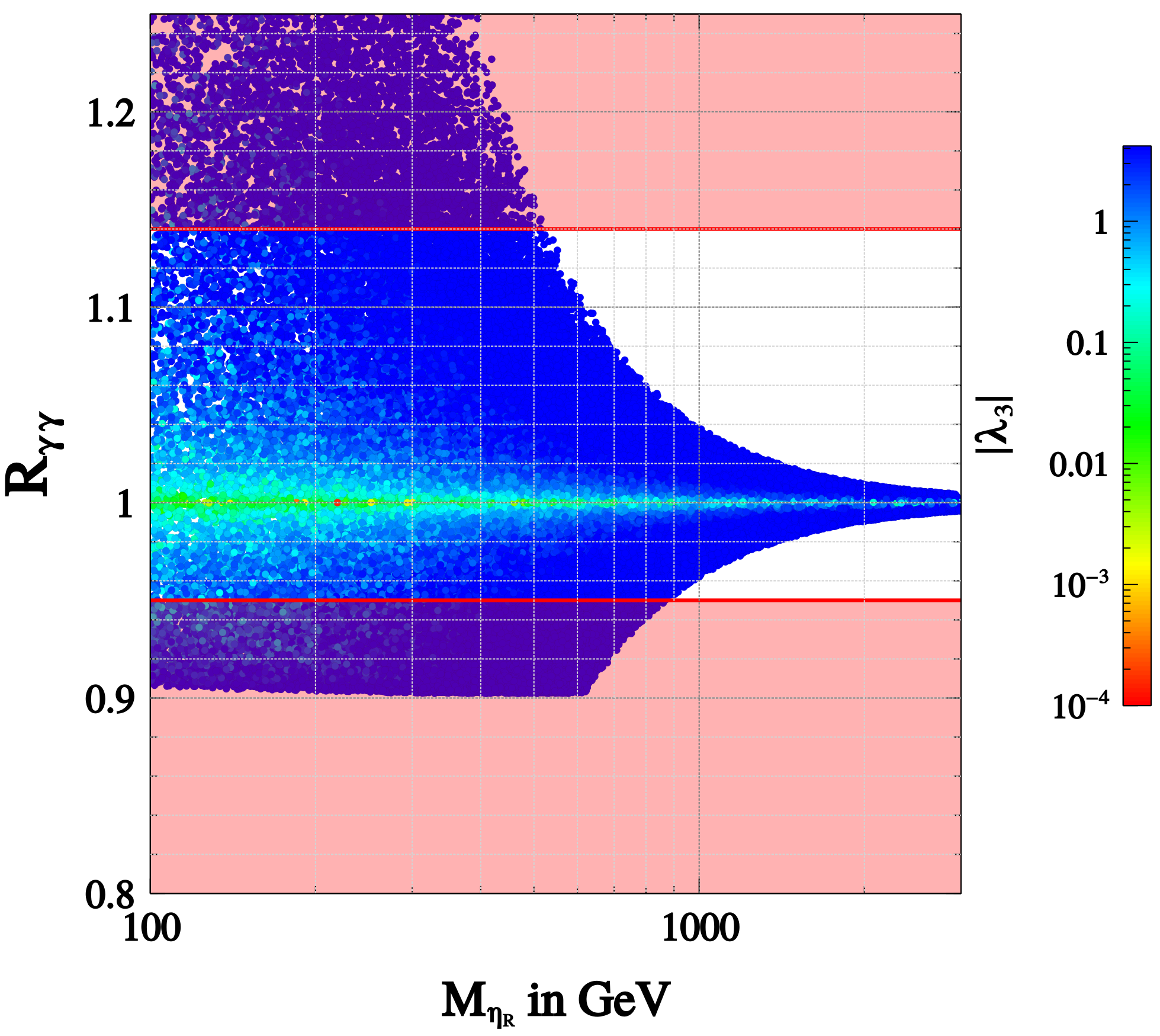
Figure 4.5: Predictions for the diphoton decay of the Higgs boson within the FSS model [175]. $R_{\gamma\gamma}$ defined in (4.19) is plotted against $m_{\eta^{+}}$ (left) and $m_{\eta_{R}}$ (right). The white region is the current experimental allowed range measured by ATLAS [537].

In Fig. 4.5, we have plotted the prediction for $R_{\gamma\gamma}$ in the context of $A_{4}$ flavor symmetric scoto-seesaw model [175] against $m_{\eta^{+}}$ (left panel) and $m_{\eta_{R}}$ (right panel). The horizontal white region ($R_{\gamma\gamma}=1.04^{+0.10}_{-0.09}$) represents the current allowed region measured by the ATLAS experiment using 139 fb^-1 of $pp$ collision data at $\sqrt{s}=13$ TeV [537]. Here $\lambda_{3}$ is a coupling for $(H^{\dagger}H)(\eta^{\dagger}\eta)$ interaction, $\eta$ being the usual inert scalar doublet appearing in scotogenic models. As we can see, a wide range of scalar boson masses can be probed through the diphoton Higgs decay channel using the present LHC experimental results. With the increasing data collection at LHC and HL-LHC, the precision of $R_{\gamma\gamma}$ will improve, giving prospects for better determination of allowed regions for specific flavor model parameters. Thus, phenomenology-based $R_{\gamma\gamma}$ constraints can be used for further studies and predictions for producing exotic discrete flavor model signals at present and future colliders.

5   Flavor Symmetry and Cosmic Frontier

In this Chapter, we will discuss some implications of flavor symmetry on various astrophysical and cosmological observables, including DM, BAU and gravitational waves.

5.1   Flavor Symmetry and Dark Matter

There is overwhelming astrophysical and cosmological evidence for the existence of DM, such as the large-scale structure data, gravitational lensing, and rotation curve of galaxies [539]. However, a laboratory discovery is still awaited. The relic abundance of DM has been measured by WMAP [540], and more recently by PLANCK [188], which set it at $26.8\%$ of the total energy budget of the Universe. However, a broad classification of DM scenarios can satisfy this condition, such as weakly interacting massive particles (WIMP) [541], feebly interacting massive particle (FIMP) [542], strongly interacting massive particle (SIMP) [543], asymmetric DM (ADM) [544], and so on. For reviews of various DM candidates, see e.g. Refs. [545, 546, 547, 548, 549]. Over the years, several attempts have been made to connect neutrino physics with DM [550, 219, 551, 552, 553, 554, 555, 556, 557, 558, 559, 560]. In a toy example [557], the authors showed a one-to-one correspondence with WIMP DM and type-I seesaw. Earlier, we discussed that discrete flavor symmetric constructions have the potential to explain neutrino masses and mixing as well as can ensure the stability of DM.

For example [158, 159], with vectorlike singlet ($\chi^{0}$)-doublet ($\psi$) DM particle spectrum assisted with additional scalars such as $\phi,\eta$ (charged under a global $U(1)$ flavor symmetry) the interaction between DM and neutrino sector can be written as

$$\mathcal{L}_{int}=\left(\frac{\phi}{\Lambda}\right)^{n}\bar{\psi}\tilde{H}\chi^{0}+\frac{(HL^{T}LH)\phi\eta}{\Lambda^{3}}.$$ (5.1)

The first term in Eq. (5.1), having a Yukawa-like configuration, acts like a Higgs portal coupling of the DM potentially accessible at various ongoing and future direct search and collider experiments. The second term in Eq. (5.1) plays a crucial role in generating non-zero $\theta_{13}$ as the existing $A_{4}$ flavons of the theory ensure the TBM mixing. A schematic view is given in Fig. 5.1.

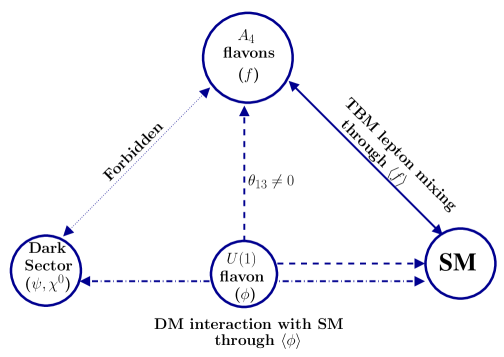
Figure 5.1: A schematic representation of DM ($\psi,\chi^{0}$) interaction with SM to generate non-zero $\theta_{13}$ in the presence of the $U(1)$ flavor symmetry. The $A_{4}$ flavons help in generating base TBM mixing. Figure adapted from the arXiv version of  Ref. [158].

Once the $U(1)$ flavor symmetry is broken, it ensures both the stability of DM and generates non-zero $\theta_{13}$. The coupling strength of the DM $\left(\frac{\phi}{\Lambda}\right)^{n}=\epsilon^{n}$ is constrained by the correct DM relic abundance, and $\epsilon$ is proportional to the magnitude of $\theta_{13}$. Additionally, the future precise measurement of the leptonic CP phase by T2K and NO$\nu$A experiments will reduce the uncertainty in $n$ [159]. Few other examples of studies of DM with discrete flavor symmetry can be found in Refs. [561, 530, 529, 562, 563, 315, 564, 565, 566, 567, 568, 569, 570].

Apart from WIMP (or freeze-out) DM paradigm, discrete flavor symmetric constructions can also be extended to the FIMP (or freeze-in) mechanism of DM. In such a scenario, non-thermal DM populating the Universe via freeze-in mechanism requires tiny dimensionless couplings ($\sim 10^{-12}$). On the other hand, if neutrinos have a tiny Dirac mass, it also requires a coupling of a similar order of magnitude. In Ref. [571], the authors have shown that such tiny coupling required in both dark and visible sectors may originate in $A_{4}$ discrete flavor symmetry. In another effort [572], it has been shown that the non-zero value of the reactor mixing angle $\theta_{13}$ can originate from Planck scale suppressed operators and can as well realize a super-WIMP DM scenario. The study of DM with non-Abelian discrete symmetries demands more attention to explore the connection between neutrino physics and DM, if any.

5.2   Flavor Symmetry and Baryon Asymmetry of the Universe

Cosmological observations reveal that our Universe possesses a net excess of baryons over antibaryons [188, 50] which is often termed as the baryon asymmetry of the Universe (BAU). This is measured by the ratio of the excess number density of baryons over antibaryons to photons at present time [188]:

$$\eta_{B}^{\rm obs}=\frac{n_{B}-n_{\bar{B}}}{n_{\gamma}}=(6.12\pm 0.08)\times 10^{-10}\,.$$ (5.2)

The mechanism of dynamical generation of the BAU is known as baryogenesis (see Refs. [573, 574, 575] for reviews) and must satisfy three basic Sakharov conditions, namely, baryon number violation, $C$ and $CP$ violation, and out-of-equilibrium [576]. Although the SM possesses all three ingredients, it is not sufficient to reproduce the observed BAU [577]. One attractive mechanism to produce the BAU is via leptogenesis [516], where one first produces a lepton asymmetry, and then uses the electroweak sphaleron processes [578, 579, 580] to convert it to a baryon asymmetry; see Refs. [581, 582, 583, 584] for reviews. This is particularly appealing, because it relies on the seesaw mechanism which also accounts for the neutrino masses and mixing, thus providing a link between the two seemingly disparate pieces of evidence for BSM physics.

In Chapter 2, we have briefly reviewed various neutrino mass generation mechanisms, which once augmented with discrete flavor symmetries explain the origin of tiny neutrino masses as well as observed neutrino mixing. Most of these mass-generation mechanisms include additional particles whose involvement also plays a crucial role in leptogenesis. The presence of various seesaw realizations of light neutrino masses in the models with discrete flavor symmetry enables us to study leptogenesis through the decay of associated heavy particles. For example, in type-I [195, 196, 199, 197, 198, 8], II [585, 8, 586, 587], and III [588] seesaw mechanisms and variants, fermion singlet RHNs ($N_{i}$), scalar triplets ($\Delta_{i}$), and fermionic triplets ($\Sigma_{i}$) are respectively included. Each scenario can potentially lead to successful leptogenesis within a wide mass range of these additional particles [589].

Resonant Leptogenesis

For example, in the case of the simple type-I seesaw, lepton asymmetry can be elegantly generated through the out-of-equilibrium decay of RHNs in the early Universe. The CP asymmetry parameter $\epsilon_{i\alpha}$ can be evaluated from the interference between the tree and one-loop level decay amplitudes of the RHN $N_{i}$ decaying into a lepton doublet $L_{\alpha}$ with specific flavor $\alpha$ and the Higgs doublet ($H$), i.e.

$$\varepsilon_{i\alpha}=\frac{\Gamma(N_{i}\to L_{\alpha}H)-\Gamma(N_{i}\to\bar{L}_{\alpha}H^{c})}{\Gamma(N_{i}\to L_{\alpha}H)+\Gamma(N_{i}\to\bar{L}_{\alpha}H^{c})}\,,$$ (5.3)

where the subscript $c$ stands for the charge conjugation. There are two types of loop-level diagrams involving vertex and wave-function corrections [590]. It turns out that the wave-function corrections can be dominant when at least two RHNs have a small mass difference comparable to their widths [591, 592, 593]. This is known as the resonant leptogenesis [471, 472], which allows the RHN mass scale to be lowered down to the electroweak-scale [594, 595, 596].

In the resonant regime, Eq. (5.3) can be written in a compact form as [472]

$$\varepsilon_{i\alpha}\simeq\frac{1}{8\pi\left(Y_{D}^{\dagger}Y_{D}\right)_{ii}}\sum_{j\neq i}{\rm Im}\Big{[}(Y_{D}^{\star})_{\alpha i}(Y_{D})_{\alpha j}\Big{]}{\rm Re}\left[\left(Y_{D}^{\dagger}Y_{D}\right)_{ij}\right]{\cal F}_{ij}\,,$$ (5.4)

where $Y_{D}$ is the Yukawa coupling matrix in the basis where the RHN mass matrix is diagonal (this is typically indicated by $\hat{Y}_{D}$, but we remove the hat for brevity). The resonant enhancement factor is given by

$${\cal F}_{ij}\,=\,\frac{M_{i}M_{j}(M_{i}^{2}-M_{j}^{2})}{(M_{i}^{2}-M_{j}^{2})^{2}+A_{ij}^{2}}.$$ (5.5)

Here the $Y_{D}$ matrices are evaluated in the RHN mass basis, and $A_{ij}$ regulates the behavior of the CP asymmetry in the limit $\Delta M_{ij}\equiv|M_{i}-M_{j}|\to 0$. As pointed out in Refs. [596, 597], in the resonant regime there are two distinct contributions to the CP asymmetry from RHN mixing and oscillation effects, both of which can be effectively captured by Eq. (5.4) but with different regulators:

$$A_{ij}^{\rm mix}\,=\,M_{i}\Gamma_{j}\,,\quad A_{ij}^{\rm osc}\,=\,(M_{i}\Gamma_{i}+M_{j}\Gamma_{j})\left[\frac{{\rm det}\left({\rm Re}\left(Y_{D}^{\dagger}Y_{D}\right)\right)}{\left(Y_{D}^{\dagger}Y_{D}\right)_{ii}\left(Y_{D}^{\dagger}Y_{D}\right)_{jj}}\right]^{1/2}\,.$$ (5.6)

The net CP asymmetry is then given by $\varepsilon_{i\alpha}^{\rm tot}=\varepsilon_{i\alpha}^{\rm mix}+\varepsilon_{i\alpha}^{\rm osc}$. This analytic approximation is in good agreement with the full quantum kinetic treatment [597, 598, 526] in the strong washout regime.

Since the regulator part is independent of the lepton flavor $\alpha$, we can sum over $\alpha$ to obtain the total CP asymmetry for a given RHN $N_{i}$:

$$\varepsilon_{i}\ \equiv\ \sum_{\alpha}\varepsilon_{i\alpha}\,=\, \frac{1}{8\pi\left(Y_{D}^{\dagger}Y_{D}\right)_{ii}}\sum_{j\neq i}{\rm Im}\left[\left(Y_{D}^{\dagger}Y_{D}\right)_{ij}\right]{\rm Re}\left[\left(Y_{D}^{\dagger}Y_{D}\right)_{ij}\right]{\cal F}_{ij}\,.$$ (5.7)

Within a semi-analytic Boltzmann approach, the flavor-dependent lepton asymmetry parameter ($\eta_{L_{\alpha}}$) can be written as [599, 595]

$$\eta_{L_{\alpha}}\simeq\frac{3}{2z_{c}K^{\rm eff}_{\alpha}}\sum_{i}\epsilon_{i\alpha}d_{i}$$ (5.8)

where $z_{c}=M_{N}/T_{c}$, $T_{c}$ is the critical temperature below which the electroweak sphalerons freeze-out, $K^{\rm eff}_{\alpha}$ are the effective washout factors and $d_{i}$ are the corresponding dilution factors given in terms of ratios of thermally-averaged rates for decays and scatterings involving the RHNs [595, 596]. The obtained lepton asymmetry then can be converted into the observed BAU via $(B+L)$-violating electroweak sphaleron processes [579, 580] which gives the final baryon asymmetry

$$\eta_{B}\simeq-0.013\sum_{\alpha}\eta_{L_{\alpha}}\,,$$ (5.9)

where the pre-factor is a product of the sphaleron conversion rate of 28/79 [580] and the entropy dilution factor of 1/27.3 [596]. It was the ratio of Eq. (5.9) to the observed value given in Eq. (5.2) plotted in Fig. 4.3.

Let us exemplify the usefulness of Eq. (5.4) by applying it to a particular case of the $\Delta(6n^{2})$ group discussed in Section 4.1 with $s$ even. We find that $\varepsilon_{3\alpha}=0$, i.e., the RHN mass eigenstate $N_{3}$ does not contribute to the CP asymmetry, and in the strong NO and IO limits,

$$\varepsilon_{1\alpha}^{\rm NO}\ \approx\ \frac{y_{2}\,y_{3}}{9}\,\left[-2\,y_{2}^{2}+y_{3}^{2}\,(1-\cos 2\,\theta_{R})\right]\,\sin 3\,\phi_{s}\sin\theta_{R}\,\sin\theta_{L,\alpha}\,\mathcal{F}_{12}\,,$$ (5.10)

$$\varepsilon_{1\alpha}^{\rm IO}\ \approx\ \frac{y_{1}\,y_{2}}{9}\,\left[-2\,y_{2}^{2}+y_{1}^{2}\,(1+\cos 2\,\theta_{R})\right]\,\sin 3\,\phi_{s}\cos\theta_{R}\,\cos\theta_{L,\alpha}\,\mathcal{F}_{12}\,,$$ (5.11)

with $\theta_{L,\alpha}=\theta_{L}+\rho_{\alpha}\,4\pi/3$ and $\rho_{e}=0$, $\rho_{\mu}=1$, $\rho_{\tau}=-1$. For strong NO (IO) $\varepsilon_{i\alpha}$ becomes very small, if $\theta_{R}\approx 0,\,\pi$ ($\theta_{R}\approx\pi/2,3\pi/2$). In addition, $\mathcal{F}_{ij}$ vanishes for $\cos 2\,\theta_{R}=0$. The CP asymmetries $\varepsilon_{2\alpha}=-\varepsilon_{1\alpha}$ with $\mathcal{F}_{12}\leftrightarrow\mathcal{F}_{21}$. For $s$ odd, similar expressions are obtained with $\sin(3\,\phi_{s})\leftrightarrow-\cos(3\,\phi_{s})$.

These analytic forms of the CP asymmetry enable us to correlate the high-and low-energy CP phases. This is illustrated in Figure 5.2 for the $\Delta(6n^{2})$ group with $n=26$, where we plot the predictions for the BAU (which depend on the high-energy CP phases) and for the $0\nu\beta\beta$ observable $m_{\beta\beta}$ (which depends on the low-energy CP phases) corresponding to the $s$ values from 0 to $n-1$. The horizontal blue-band corresponds to $\eta_{B}$ values within 10% of the observed value. We find that there exist some $s$ values for which the correct BAU can be obtained, while the $m_{\beta\beta}$ predictions for the IO case are either already excluded or will be tested soon in the next-generation $0\nu\beta\beta$ experiments.

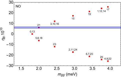
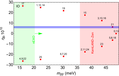
Figure 5.2: Correlation between the predicted BAU $\eta_{B}$ and the effective neutrino mass $m_{\beta\beta}$ for a $\Delta(6n^{2})$ model with $n=26$ and $0\leq s\leq n-1$ (as shown by the numbered points). The blue-shaded horizontal bar corresponds to $\eta_{B}$ within $10\%$ of $\eta_{B}^{\rm obs}$ [188]. The vertical shaded bands for the IO case indicate the smallest $m_{\beta\beta}$ value (including the NME uncertainties) that is either ruled out by KamLAND-Zen [48] (red) or will be accessible to nEXO [49] (green). Figure taken from Ref. [464].

ARS Mechanism and Unified Picture

Just like the case with DM relic density which can happen either by freeze-out or freeze-in, the deviation from equilibrium for the RHNs can also happen either via freeze-out when their mass drops below the Hubble temperature), or via freeze-in when the Yukawa couplings are so small that the equilibration rate becomes much lower than the Hubble rate. The resonant leptogenesis mechanism discussed above is an example of the freeze-out scenario, while leptogenesis via oscillations (the so-called ARS mechanism) [600] is an example of the freeze-in scenario, which typically happens for GeV-scale RHNs [601, 602, 603, 604]. These two mechanisms may seem to be quite different, but it was recently shown that both can be described in a unified picture [605, 527, 526]. This can be achieved with matrix-valued quantum kinetic equations for the RHNs and the lepton asymmetries in different SM degrees of freedom. Solving these equations for RHN masses in a wide range from 50 MeV to 70 TeV, Ref. [606] obtained the range of total mixing angle $U^{2}$ consistent with leptogenesis, as shown in Fig. 5.3. Here $\kappa$ refers to the RHN mass splitting parameter, and the contours corrersponding to positive (negative) BAU are shown by solid (dashed) lines. The black line indicates the canonical seesaw line. The red and blue shaded regions lead to unacceptably large corrections to the light neutrino masses induced by the RHN mass splitting.

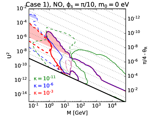
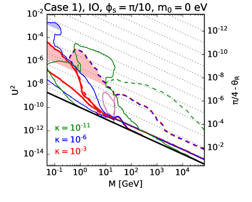
Figure 5.3: Range of total mixing angle $U^{2}$ consistent with leptogenesis for a wide range of RHN mass in a $\Delta(6n^{2})$ model. Figure taken from the arXiv version of Ref. [606].

Other Examples

As mentioned earlier, in models with discrete flavor symmetry, structures of the Dirac Yukawa coupling, charged lepton and RHN mass matrices are entirely instrumented by the associated symmetry. Hence, the involved discrete symmetry may have a significant impact on neutrino masses, mixing, and Dirac CP phase as well high energy CP violation required for leptogenesis. As TBM mixing was a potential candidate for the lepton mixing matrix, several analyses have been performed to explain TBM mixing and leptogenesis [607, 242, 608]. Interestingly, it was also observed [607] that in the exact TBM limit, the CP asymmetry vanishes since ${Y}^{\dagger}_{D}{Y}_{D}\propto\mathbb{I}$ (where ${Y}_{D}$ in the Dirac Yukawa coupling in the basis where RHNs are diagonal). Therefore in the exact TBM scenario, leptogenesis was realized either by introducing higher-order correction in the Dirac Yukawa matrix [607, 242] or by introducing renormalization group effects [608]; see however Ref. [609] which derived a no-go theorem for the viability of the minimal radiative resonant leptogenesis. In the precision era of the neutrino mixing parameters, it is essential to study the effect of non-zero $\theta_{13}$ and CP phases. In the $A_{4}$ type-I seesaw scenario [155], the authors showed that a minimal (by adding a non-trivial $A_{4}$ singlet) modification to the existing Altarelli-Feruglio [114] model may give rise to non-zero $\theta_{13}$ as well as generate the observed BAU. Here, the high-energy CP phases or the Majorana phases appearing in the CP asymmetry also get constrained by the low-energy neutrino oscillation data, which are otherwise insensitive to the oscillation experiments. In a more minimal study [201], the authors showed that with the presence of only three $A_{4}$ flavons, both non-zero $\theta_{13}$ and BAU (incorporating renormalization group effects) can be generated. To unify all the sources of CP violation in the theory, the CP symmetry can be spontaneously broken by the VEV of a singlet field where its magnitude generates non-zero $\theta_{13}$ and the phase factor becomes directly proportional to the CP asymmetry parameter in general $A_{4}$ type-I+II scenario [156]. Recently, it has also been shown that BAU can be successfully generated in a $S_{4}$ discrete symmetry framework with TM₁ mixing [177] taking lepton flavor effects into consideration. Apart from the example discussed here for $\Delta(6\,n^{2})$, a few other works exploring leptogenesis in similar flavor symmetry models are Refs. [610, 611, 612, 606]. For more recent studies on various discrete flavor symmetry and leptogenesis, see Refs. [613, 371, 614, 615, 616, 617, 618].

5.3   Flavor Symmetry and Gravitational Waves

The recent breakthrough in gravitational wave (GW) observations by LIGO [619] provides us a new window into the early universe. A particularly interesting example of early Universe phenomena that can be a stochastic source of GWs is cosmological phase transition [620] whose observation may shed light on an array of BSM phenomena, from BAU to GUT physics and inflation [621]. As the Majorana mass term in neutrino mass models can be generated by $B-L$ breaking at a high energy scale, the associated phase transition in the early Universe can produce a possibly observable stochastic GW background, thus providing a complementary probe of $B-L$ physics like leptogenesis [622, 623, 624, 625].

As for the discrete flavor symmetry models, a direct test would be the observation of flavons involved in the spontaneous breaking of the discrete symmetry. This is usually assumed to happen at a high scale, which makes it challenging to test experimentally. Whatever the scale of the discrete flavor symmetry spontaneous breaking, it gives rise to degenerate vacua separated by energy barriers leading to a network of cosmic domain walls. This is a serious problem, if the walls are stable, as they could overclose the Universe [626, 627]. Solutions to this domain wall problem have been discussed in the context of non-Abelian discrete symmetries such as $A_{4}$, which include explicit breaking terms, such that the domain walls collapse in a certain period of time before the symmetry breaking [628, 629, 630]. Such collapse of domain walls in the early Universe could lead to stochastic GWs [631, 632, 633, 634, 635], thus offering novel probes to test the discrete flavor symmetry models at current and future GW experiments (such as aLIGO/VIRGO, LISA, DECIGO, BBO, ET and CE) [636]. See also Ref. [637] for other GW imprints of flavor models, such as multipeaked stochastic GW signal from a series of cosmological phase transitions that could be a unique probe of the mechanism behind flavor hierarchies.

6   Summary and Outlook

The origin of neutrino masses and mixing is a fundamental question in particle physics. In this review, we have discussed flavor model building strategies based on discrete family symmetries aimed at explaining the patterns of lepton masses and flavor mixing. We consider fixed patterns (BM, TBM, GR, HG) and more elaborate symmetry groups with unbroken residual symmetries (e.g., $A_{4}$, $S_{4}$, $A_{5}$, $T^{\prime}$, $\Delta(27)$, $\Delta(6n^{2})$), motivated by the increasingly precise results from neutrino oscillation experiments. In particular, a ‘large’ reactor mixing angle $\theta_{13}$ has been determined, the Dirac CP phase $\delta$ is preferred to be nonzero and the normal mass ordering seems to be mildly favored in the current oscillation data. We discuss the far-reaching implications of these considerations in flavor model building and phenomenology. We also discussed flavor symmetry breaking and mechanisms of mass generation, and flavor symmetry in multi-Higgs doublet models.

As there are plenty (hundreds) of possible flavor symmetry models, a natural question is: How to falsify or validate any of these models? Generally, such symmetries are broken at a high scale and beyond our experimental reach. Nonetheless, phenomenological study connected with flavor symmetry effects is rich and models can be probed effectively in low-energy intensity frontier experiments (like neutrino oscillation experiments, neutrinoless double beta decay, and lepton flavor violation searches), high energy colliders (such as LHC and future lepton/hadron colliders), as well as at the cosmological frontier (via baryogenesis, dark matter and stochastic gravitational wave signals). One of the key tests for such models comes from the seesaw mechanism, namely, the presence of heavy right-handed Majorana neutrinos. Their Yukawa couplings are relevant for collider signals, LFV and leptogenesis. We give an example of such studies for the $\Delta(6n^{2})$ group. Other groups (e.g. $A_{4}$) and models (e.g. scotogenic) are also discussed in the context of LFV and dark matter effects.

The concept of flavor symmetry is developing all the time. New ideas related to family symmetries also come from modular symmetries or texture zeroes. In the review, we have updated many strict correlations and predictions in models based on TM₁, TM₂ mixing, $\mu-\tau$ reflection symmetries and status of light neutrino mass sum rules in the context of neutrinoless double beta decay. However, given the plethora of flavor models and the rich phenomenology they offer, we cannot discuss all possibilities here. Our goal in this review was to give a gist of the flurry of activities going on in this field, illustrated with a few example scenarios. With neutrino physics entering the precision era, there is an exciting prospect for more intensive studies of discrete flavor symmetries in the future for Majorana and Dirac neutrino scenarios.

Appendix A $A_{4}$ symmetry

The $A_{4}$ discrete symmetry group is a group of even permutations of four objects. Geometrically, it can be considered as an invariance group of a tetrahedron. It has 12 elements which can be generated by two basic objects $S$ and $T$ which obey the relation $S^{2}=T^{3}=(ST)^{3}=1$.

The $A_{4}$ group has three one-dimensional irreducible representations $1$,$1^{\prime}$ and $1^{\prime\prime}$ and one three dimensional irreducible representation 3. For a detailed discussion on $A_{4}$ character table and three-dimensional unitary representation of the generators, see Refs. [78, 77]. The multiplication rules of the singlets and triplets are given by [78, 77]

$$1 \otimes 1=1;~{}1^{\prime}\otimes 1^{\prime\prime}=1,$$ (A.1)

$$1^{\prime} \otimes 1^{\prime}=1^{\prime\prime};~{}1^{\prime\prime}\otimes 1^{\prime\prime}=1^{\prime},$$ (A.2)

$$3 \otimes 3=1\oplus 1^{\prime}\oplus 1^{\prime\prime}\oplus 3_{s}\oplus 3_{a},$$ (A.3)

where the subscripts $``s"$ and $``a"$ denote symmetric and antisymmetric part respectively. In the $T$ diagonal basis [78], writing two triplets as $(x_{1},x_{2},x_{3})$ and $(y_{1},y_{2},y_{3})$ respectively, we can write their products explicitly as

$$1 \sim x_{1}y_{1}+x_{2}y_{3}+x_{3}y_{2},$$ (A.4)

$$1^{\prime} \sim x_{3}y_{3}+x_{1}y_{2}+x_{2}y_{1},$$ (A.5)

$$1^{\prime\prime} \sim x_{2}y_{2}+x_{1}y_{3}+x_{3}y_{1},$$ (A.6)

$$3_{s} \sim \frac{1}{3}\begin{pmatrix}2x_{1}y_{1}-x_{2}y_{3}-x_{3}y_{2}\\ 2x_{3}y_{3}-x_{1}y_{2}-x_{2}y_{1}\\ 2x_{2}y_{2}-x_{1}y_{3}-x_{3}y_{1}\end{pmatrix},$$ (A.7)

$$3_{a} \sim \frac{1}{2}\begin{pmatrix}x_{2}y_{3}-x_{3}y_{2}\\ x_{1}y_{2}-x_{2}y_{1}\\ x_{3}y_{1}-x_{1}y_{3}\end{pmatrix}.$$ (A.8)

References

- [1] V. D. Barger, K. Whisnant, Majorana neutrino masses from neutrinoless double beta decay and cosmology, Phys. Lett. B 456 (1999) 194–200. arXiv:hep-ph/9904281, doi:10.1016/S0370-2693(99)00514-6.
- [2] M. Czakon, J. Gluza, M. Zralek, Nature of neutrinos in the light of present and future experiments, Phys. Lett. B 465 (1999) 211–218. arXiv:hep-ph/9906381, doi:10.1016/S0370-2693(99)01008-4.
- [3] R. Davis, Jr., D. S. Harmer, K. C. Hoffman, Search for neutrinos from the Sun, Phys. Rev. Lett. 20 (1968) 1205–1209. doi:10.1103/PhysRevLett.20.1205.
- [4] J. N. Bahcall, R. Davis, Solar Neutrinos - a Scientific Puzzle, Science 191 (1976) 264–267. doi:10.1126/science.191.4224.264.
- [5] Y. Fukuda, et al., Evidence for oscillation of atmospheric neutrinos, Phys. Rev. Lett. 81 (1998) 1562–1567. arXiv:hep-ex/9807003, doi:10.1103/PhysRevLett.81.1562.
- [6] Q. R. Ahmad, et al., Measurement of the rate of interactions produced by 8B solar neutrinos at the Sudbury Neutrino Observatory, Phys. Rev. Lett. 87 (2001) 071301. arXiv:nucl-ex/0106015, doi:10.1103/PhysRevLett.87.071301.
- [7] Q. R. Ahmad, et al., Direct evidence for neutrino flavor transformation from neutral current interactions in the Sudbury Neutrino Observatory, Phys. Rev. Lett. 89 (2002) 011301. arXiv:nucl-ex/0204008, doi:10.1103/PhysRevLett.89.011301.
- [8] J. Schechter, J. W. F. Valle, Neutrino Masses in SU(2) x U(1) Theories, Phys. Rev. D 22 (1980) 2227. doi:10.1103/PhysRevD.22.2227.
- [9] J. Schechter, J. W. F. Valle, Neutrino Oscillation Thought Experiment, Phys. Rev. D 23 (1981) 1666. doi:10.1103/PhysRevD.23.1666.
- [10] W. Rodejohann, J. W. F. Valle, Symmetrical Parametrizations of the Lepton Mixing Matrix, Phys. Rev. D 84 (2011) 073011. arXiv:1108.3484, doi:10.1103/PhysRevD.84.073011.
- [11] B. Pontecorvo, Inverse beta processes and nonconservation of lepton charge, Zh. Eksp. Teor. Fiz. 34 (1957) 247.
- [12] Z. Maki, M. Nakagawa, S. Sakata, Remarks on the unified model of elementary particles, Prog. Theor. Phys. 28 (1962) 870–880. doi:10.1143/PTP.28.870.
- [13] M. Kobayashi, T. Maskawa, CP Violation in the Renormalizable Theory of Weak Interaction, Prog. Theor. Phys. 49 (1973) 652–657. doi:10.1143/PTP.49.652.
- [14] R. L. Workman, et al., Review of Particle Physics, Progress of Theoretical and Experimental Physics 2022 (8) (2022) 083C01, Neutrino Masses, Mixing, and Oscillations. doi:10.1093/ptep/ptac097.
- [15] J. Gluza, M. Zralek, Parameters’ domain in three flavor neutrino oscillations, Phys. Lett. B 517 (2001) 158–166. arXiv:hep-ph/0106283, doi:10.1016/S0370-2693(01)00962-5.
- [16] S. Roy, N. N. Singh, A model-independent investigation on quasi-degenerate neutrino mass models and their significance, Nucl. Phys. B 877 (2013) 321–342. arXiv:1603.07246, doi:10.1016/j.nuclphysb.2013.10.011.
- [17] G. L. Fogli, E. Lisi, A. Marrone, D. Montanino, A. Palazzo, Getting the most from the statistical analysis of solar neutrino oscillations, Phys. Rev. D 66 (2002) 053010. arXiv:hep-ph/0206162, doi:10.1103/PhysRevD.66.053010.
- [18] O. G. Miranda, M. A. Tortola, J. W. F. Valle, Are solar neutrino oscillations robust?, JHEP 10 (2006) 008. arXiv:hep-ph/0406280, doi:10.1088/1126-6708/2006/10/008.
- [19] Nufit 5.2, http://www.nu-fit.org/ (2022).
- [20] I. Esteban, M. C. Gonzalez-Garcia, M. Maltoni, T. Schwetz, A. Zhou, The fate of hints: updated global analysis of three-flavor neutrino oscillations, JHEP 09 (2020) 178. arXiv:2007.14792, doi:10.1007/JHEP09(2020)178.
- [21] P. F. de Salas, D. V. Forero, S. Gariazzo, P. Martínez-Miravé, O. Mena, C. A. Ternes, M. Tórtola, J. W. F. Valle, 2020 global reassessment of the neutrino oscillation picture, JHEP 02 (2021) 071. arXiv:2006.11237, doi:10.1007/JHEP02(2021)071.
- [22] P. F. De Salas, D. V. Forero, S. Gariazzo, P. Martínez-Miravé, O. Mena, C. A. Ternes, M. Tórtola, J. W. F. Valle, Chi2 profiles from Valencia neutrino global fit, http://globalfit.astroparticles.es/ (2021). doi:10.5281/zenodo.4726908.
- [23] F. Capozzi, E. Di Valentino, E. Lisi, A. Marrone, A. Melchiorri, A. Palazzo, Unfinished fabric of the three neutrino paradigm, Phys. Rev. D 104 (8) (2021) 083031. arXiv:2107.00532, doi:10.1103/PhysRevD.104.083031.
- [24] Y. Nakajima, Recent results and future prospects from Super- Kamiokande (Jun. 2020). doi:10.5281/zenodo.4134680.
- [25] V. Takhistov, Review of Atmospheric Neutrino Results from Super-Kamiokande, PoS ICHEP2020 (2021) 181. arXiv:2012.06864, doi:10.22323/1.390.0181.
- [26] S. F. King, C. Luhn, Neutrino Mass and Mixing with Discrete Symmetry, Rept. Prog. Phys. 76 (2013) 056201. arXiv:1301.1340, doi:10.1088/0034-4885/76/5/056201.
- [27] S. K. Agarwalla, R. Kundu, S. Prakash, M. Singh, A close look on 2-3 mixing angle with DUNE in light of current neutrino oscillation data, JHEP 03 (2022) 206. arXiv:2111.11748, doi:10.1007/JHEP03(2022)206.
- [28] K. Abe, et al., Constraint on the matter–antimatter symmetry-violating phase in neutrino oscillations, Nature 580 (7803) (2020) 339–344, [Erratum: Nature 583, E16 (2020)]. arXiv:1910.03887, doi:10.1038/s41586-020-2177-0.
- [29] K. Abe, et al., Improved constraints on neutrino mixing from the T2K experiment with protons on target, Phys. Rev. D 103 (11) (2021) 112008. arXiv:2101.03779, doi:10.1103/PhysRevD.103.112008.
- [30] K. Abe, et al., Measurements of neutrino oscillation parameters from the T2K experiment using protons on target, Eur. Phys. J. C 83 (9) (2023) 782. arXiv:2303.03222, doi:10.1140/epjc/s10052-023-11819-x.
- [31] M. A. Acero, et al., Improved measurement of neutrino oscillation parameters by the NOvA experiment, Phys. Rev. D 106 (3) (2022) 032004. arXiv:2108.08219, doi:10.1103/PhysRevD.106.032004.
- [32] U. Rahaman, S. Razzaque, S. U. Sankar, A Review of the Tension between the T2K and NOA Appearance Data and Hints to New Physics, Universe 8 (2) (2022) 109. arXiv:2201.03250, doi:10.3390/universe8020109.
- [33] P. B. Denton, M. Friend, M. D. Messier, H. A. Tanaka, S. Böser, J. a. A. B. Coelho, M. Perrin-Terrin, T. Stuttard, Snowmass Neutrino Frontier: NF01 Topical Group Report on Three-Flavor Neutrino Oscillations (12 2022). arXiv:2212.00809.
- [34] Z. Djurcic, et al., JUNO Conceptual Design Report (8 2015). arXiv:1508.07166.
- [35] K. Abe, et al., Hyper-Kamiokande Design Report (5 2018). arXiv:1805.04163.
- [36] B. Abi, et al., Deep Underground Neutrino Experiment (DUNE), Far Detector Technical Design Report, Volume I Introduction to DUNE, JINST 15 (08) (2020) T08008. arXiv:2002.02967, doi:10.1088/1748-0221/15/08/T08008.
- [37] M. G. Aartsen, et al., Combined sensitivity to the neutrino mass ordering with JUNO, the IceCube Upgrade, and PINGU, Phys. Rev. D 101 (3) (2020) 032006. arXiv:1911.06745, doi:10.1103/PhysRevD.101.032006.
- [38] H. Minakata, H. Nunokawa, A. A. Quiroga, Constraining Majorana CP phase in the precision era of cosmology and the double beta decay experiment, PTEP 2015 (2015) 033B03. arXiv:1402.6014, doi:10.1093/ptep/ptv010.
- [39] I. Girardi, S. T. Petcov, A. V. Titov, Predictions for the Majorana CP Violation Phases in the Neutrino Mixing Matrix and Neutrinoless Double Beta Decay, Nucl. Phys. B 911 (2016) 754–804. arXiv:1605.04172, doi:10.1016/j.nuclphysb.2016.08.019.
- [40] J. A. Formaggio, A. L. C. de Gouvêa, R. G. H. Robertson, Direct Measurements of Neutrino Mass, Phys. Rept. 914 (2021) 1–54. arXiv:2102.00594, doi:10.1016/j.physrep.2021.02.002.
- [41] M. J. Dolinski, A. W. P. Poon, W. Rodejohann, Neutrinoless Double-Beta Decay: Status and Prospects, Ann. Rev. Nucl. Part. Sci. 69 (2019) 219–251. arXiv:1902.04097, doi:10.1146/annurev-nucl-101918-023407.
- [42] M. Archidiacono, S. Hannestad, J. Lesgourgues, What will it take to measure individual neutrino mass states using cosmology?, JCAP 09 (2020) 021. arXiv:2003.03354, doi:10.1088/1475-7516/2020/09/021.
- [43] I. Esteban, M. C. Gonzalez-Garcia, A. Hernandez-Cabezudo, M. Maltoni, T. Schwetz, Global analysis of three-flavour neutrino oscillations: synergies and tensions in the determination of , , and the mass ordering, JHEP 01 (2019) 106. arXiv:1811.05487, doi:10.1007/JHEP01(2019)106.
- [44] M. Aker, et al., Direct neutrino-mass measurement with sub-electronvolt sensitivity, Nature Phys. 18 (2) (2022) 160–166. arXiv:2105.08533, doi:10.1038/s41567-021-01463-1.
- [45] M. Aker, et al., The design, construction, and commissioning of the KATRIN experiment, JINST 16 (08) (2021) T08015. arXiv:2103.04755, doi:10.1088/1748-0221/16/08/T08015.
- [46] A. A. Esfahani, et al., The Project 8 Neutrino Mass Experiment, in: Snowmass 2021, 2022. arXiv:2203.07349.
- [47] A. Ashtari Esfahani, et al., Tritium Beta Spectrum Measurement and Neutrino Mass Limit from Cyclotron Radiation Emission Spectroscopy, Phys. Rev. Lett. 131 (10) (2023) 102502. arXiv:2212.05048, doi:10.1103/PhysRevLett.131.102502.
- [48] S. Abe, et al., Search for the Majorana Nature of Neutrinos in the Inverted Mass Ordering Region with KamLAND-Zen, Phys. Rev. Lett. 130 (5) (2023) 051801. arXiv:2203.02139, doi:10.1103/PhysRevLett.130.051801.
- [49] G. Adhikari, et al., nEXO: neutrinoless double beta decay search beyond 1028 year half-life sensitivity, J. Phys. G 49 (1) (2022) 015104. arXiv:2106.16243, doi:10.1088/1361-6471/ac3631.
- [50] N. Aghanim, et al., Planck 2018 results. VI. Cosmological parameters, Astron. Astrophys. 641 (2020) A6, [Erratum: Astron.Astrophys. 652, C4 (2021)]. arXiv:1807.06209, doi:10.1051/0004-6361/201833910.
- [51] C. Adams, et al., Neutrinoless Double Beta Decay (12 2022). arXiv:2212.11099.
- [52] M. Agostini, et al., Final Results of GERDA on the Search for Neutrinoless Double- Decay, Phys. Rev. Lett. 125 (25) (2020) 252502. arXiv:2009.06079, doi:10.1103/PhysRevLett.125.252502.
- [53] N. Abgrall, et al., The Large Enriched Germanium Experiment for Neutrinoless Decay: LEGEND-1000 Preconceptual Design Report (7 2021). arXiv:2107.11462.
- [54] M. Askins, et al., THEIA: an advanced optical neutrino detector, Eur. Phys. J. C 80 (5) (2020) 416. arXiv:1911.03501, doi:10.1140/epjc/s10052-020-7977-8.
- [55] J. Lesgourgues, S. Pastor, Massive neutrinos and cosmology, Phys. Rept. 429 (2006) 307–379. arXiv:astro-ph/0603494, doi:10.1016/j.physrep.2006.04.001.
- [56] N. Palanque-Delabrouille, C. Yèche, N. Schöneberg, J. Lesgourgues, M. Walther, S. Chabanier, E. Armengaud, Hints, neutrino bounds and WDM constraints from SDSS DR14 Lyman- and Planck full-survey data, JCAP 04 (2020) 038. arXiv:1911.09073, doi:10.1088/1475-7516/2020/04/038.
- [57] E. Di Valentino, S. Gariazzo, O. Mena, Most constraining cosmological neutrino mass bounds, Phys. Rev. D 104 (8) (2021) 083504. arXiv:2106.15267, doi:10.1103/PhysRevD.104.083504.
- [58] E. Di Valentino, A. Melchiorri, Neutrino Mass Bounds in the Era of Tension Cosmology, Astrophys. J. Lett. 931 (2) (2022) L18. arXiv:2112.02993, doi:10.3847/2041-8213/ac6ef5.
- [59] K. N. Abazajian, et al., Neutrino Physics from the Cosmic Microwave Background and Large Scale Structure, Astropart. Phys. 63 (2015) 66–80. arXiv:1309.5383, doi:10.1016/j.astropartphys.2014.05.014.
- [60] C. L. Chang, et al., Snowmass2021 Cosmic Frontier: Cosmic Microwave Background Measurements White Paper (3 2022). arXiv:2203.07638.
- [61] Z.-z. Xing, The µ– reflection symmetry of Majorana neutrinos ∗, Rept. Prog. Phys. 86 (7) (2023) 076201. arXiv:2210.11922, doi:10.1088/1361-6633/acd8ce.
- [62] F. P. An, et al., Observation of electron-antineutrino disappearance at Daya Bay, Phys. Rev. Lett. 108 (2012) 171803. arXiv:1203.1669, doi:10.1103/PhysRevLett.108.171803.
- [63] J. K. Ahn, et al., Observation of Reactor Electron Antineutrino Disappearance in the RENO Experiment, Phys. Rev. Lett. 108 (2012) 191802. arXiv:1204.0626, doi:10.1103/PhysRevLett.108.191802.
- [64] F. Vissani, A Study of the scenario with nearly degenerate Majorana neutrinos (8 1997). arXiv:hep-ph/9708483.
- [65] M. Fukugita, M. Tanimoto, T. Yanagida, Atmospheric neutrino oscillation and a phenomenological lepton mass matrix, Phys. Rev. D 57 (1998) 4429–4432. arXiv:hep-ph/9709388, doi:10.1103/PhysRevD.57.4429.
- [66] V. D. Barger, S. Pakvasa, T. J. Weiler, K. Whisnant, Bimaximal mixing of three neutrinos, Phys. Lett. B 437 (1998) 107–116. arXiv:hep-ph/9806387, doi:10.1016/S0370-2693(98)00880-6.
- [67] A. J. Baltz, A. S. Goldhaber, M. Goldhaber, The Solar neutrino puzzle: An Oscillation solution with maximal neutrino mixing, Phys. Rev. Lett. 81 (1998) 5730–5733. arXiv:hep-ph/9806540, doi:10.1103/PhysRevLett.81.5730.
- [68] P. F. Harrison, D. H. Perkins, W. G. Scott, Tri-bimaximal mixing and the neutrino oscillation data, Phys. Lett. B 530 (2002) 167. arXiv:hep-ph/0202074, doi:10.1016/S0370-2693(02)01336-9.
- [69] P. F. Harrison, W. G. Scott, Symmetries and generalizations of tri - bimaximal neutrino mixing, Phys. Lett. B 535 (2002) 163–169. arXiv:hep-ph/0203209, doi:10.1016/S0370-2693(02)01753-7.
- [70] C. H. Albright, A. Dueck, W. Rodejohann, Possible Alternatives to Tri-bimaximal Mixing, Eur. Phys. J. C 70 (2010) 1099–1110. arXiv:1004.2798, doi:10.1140/epjc/s10052-010-1492-2.
- [71] A. Datta, F.-S. Ling, P. Ramond, Correlated hierarchy, Dirac masses and large mixing angles, Nucl. Phys. B 671 (2003) 383–400. arXiv:hep-ph/0306002, doi:10.1016/j.nuclphysb.2003.08.026.
- [72] Y. Kajiyama, M. Raidal, A. Strumia, The Golden ratio prediction for the solar neutrino mixing, Phys. Rev. D 76 (2007) 117301. arXiv:0705.4559, doi:10.1103/PhysRevD.76.117301.
- [73] L. L. Everett, A. J. Stuart, Icosahedral (A(5)) Family Symmetry and the Golden Ratio Prediction for Solar Neutrino Mixing, Phys. Rev. D 79 (2009) 085005. arXiv:0812.1057, doi:10.1103/PhysRevD.79.085005.
- [74] W. Rodejohann, Unified Parametrization for Quark and Lepton Mixing Angles, Phys. Lett. B 671 (2009) 267–271. arXiv:0810.5239, doi:10.1016/j.physletb.2008.12.010.
- [75] A. Adulpravitchai, A. Blum, W. Rodejohann, Golden Ratio Prediction for Solar Neutrino Mixing, New J. Phys. 11 (2009) 063026. arXiv:0903.0531, doi:10.1088/1367-2630/11/6/063026.
- [76] G.-J. Ding, L. L. Everett, A. J. Stuart, Golden Ratio Neutrino Mixing and Flavor Symmetry, Nucl. Phys. B 857 (2012) 219–253. arXiv:1110.1688, doi:10.1016/j.nuclphysb.2011.12.004.
- [77] H. Ishimori, T. Kobayashi, H. Ohki, Y. Shimizu, H. Okada, M. Tanimoto, Non-Abelian Discrete Symmetries in Particle Physics, Prog. Theor. Phys. Suppl. 183 (2010) 1–163. arXiv:1003.3552, doi:10.1143/PTPS.183.1.
- [78] G. Altarelli, F. Feruglio, Discrete Flavor Symmetries and Models of Neutrino Mixing, Rev. Mod. Phys. 82 (2010) 2701–2729. arXiv:1002.0211, doi:10.1103/RevModPhys.82.2701.
- [79] D. Wyler, Discrete Symmetries in the Six Quark SU(2) X U(1) Model, Phys. Rev. D 19 (1979) 3369. doi:10.1103/PhysRevD.19.3369.
- [80] G. C. Branco, H. P. Nilles, V. Rittenberg, Fermion Masses and Hierarchy of Symmetry Breaking, Phys. Rev. D 21 (1980) 3417. doi:10.1103/PhysRevD.21.3417.
- [81] Y. Abe, et al., Indication of Reactor Disappearance in the Double Chooz Experiment, Phys. Rev. Lett. 108 (2012) 131801. arXiv:1112.6353, doi:10.1103/PhysRevLett.108.131801.
- [82] K. Abe, et al., Observation of Electron Neutrino Appearance in a Muon Neutrino Beam, Phys. Rev. Lett. 112 (2014) 061802. arXiv:1311.4750, doi:10.1103/PhysRevLett.112.061802.
- [83] P. Adamson, et al., Measurement of Neutrino and Antineutrino Oscillations Using Beam and Atmospheric Data in MINOS, Phys. Rev. Lett. 110 (25) (2013) 251801. arXiv:1304.6335, doi:10.1103/PhysRevLett.110.251801.
- [84] S. Gariazzo, C. Giunti, M. Laveder, Neutrino Unbound, http://www.nu.to.infn.it/ (2020).
- [85] W. Flieger, J. Gluza, General neutrino mass spectrum and mixing properties in seesaw mechanisms, Chin. Phys. C 45 (2) (2021) 023106. arXiv:2004.00354, doi:10.1088/1674-1137/abcd2f.
- [86] S. A. R. Ellis, K. J. Kelly, S. W. Li, Current and Future Neutrino Oscillation Constraints on Leptonic Unitarity, JHEP 12 (2020) 068. arXiv:2008.01088, doi:10.1007/JHEP12(2020)068.
- [87] M. Bona, et al., New UTfit Analysis of the Unitarity Triangle in the Cabibbo-Kobayashi-Maskawa scheme, Rend. Lincei Sci. Fis. Nat. 34 (2023) 37–57. arXiv:2212.03894, doi:10.1007/s12210-023-01137-5.
- [88] K. Bielas, W. Flieger, J. Gluza, M. Gluza, Neutrino mixing, interval matrices and singular values, Phys. Rev. D 98 (5) (2018) 053001. arXiv:1708.09196, doi:10.1103/PhysRevD.98.053001.
- [89] W. Flieger, J. Gluza, K. Porwit, New limits on neutrino non-unitary mixings based on prescribed singular values, JHEP 03 (2020) 169. arXiv:1910.01233, doi:10.1007/JHEP03(2020)169.
- [90] S. T. Petcov, Discrete Flavour Symmetries, Neutrino Mixing and Leptonic CP Violation, Eur. Phys. J. C 78 (9) (2018) 709. arXiv:1711.10806, doi:10.1140/epjc/s10052-018-6158-5.
- [91] F. Feruglio, A. Romanino, Lepton flavor symmetries, Rev. Mod. Phys. 93 (1) (2021) 015007. arXiv:1912.06028, doi:10.1103/RevModPhys.93.015007.
- [92] P. H. Frampton, T. W. Kephart, Simple nonAbelian finite flavor groups and fermion masses, Int. J. Mod. Phys. A 10 (1995) 4689–4704. arXiv:hep-ph/9409330, doi:10.1142/S0217751X95002187.
- [93] Z.-z. Xing, Flavor structures of charged fermions and massive neutrinos, Phys. Rept. 854 (2020) 1–147. arXiv:1909.09610, doi:10.1016/j.physrep.2020.02.001.
- [94] R. de Adelhart Toorop, F. Feruglio, C. Hagedorn, Finite Modular Groups and Lepton Mixing, Nucl. Phys. B 858 (2012) 437–467. arXiv:1112.1340, doi:10.1016/j.nuclphysb.2012.01.017.
- [95] M. Tanimoto, Neutrinos and flavor symmetries, AIP Conf. Proc. 1666 (1) (2015) 120002. doi:10.1063/1.4915578.
- [96] Z.-z. Xing, Z.-h. Zhao, A review of - flavor symmetry in neutrino physics, Rept. Prog. Phys. 79 (7) (2016) 076201. arXiv:1512.04207, doi:10.1088/0034-4885/79/7/076201.
- [97] S. F. King, Neutrino physics - a review, PoS CORFU2019 (2020) 030. doi:10.22323/1.376.0030.
- [98] M. Sajjad Athar, et al., Status and perspectives of neutrino physics, Prog. Part. Nucl. Phys. 124 (2022) 103947. arXiv:2111.07586, doi:10.1016/j.ppnp.2022.103947.
- [99] J. Gehrlein, S. Petcov, M. Spinrath, A. Titov, Testing neutrino flavor models, in: Snowmass 2021, 2022. arXiv:2203.06219.
- [100] W. Altmannshofer, J. Zupan, Snowmass White Paper: Flavor Model Building, in: Snowmass 2021, 2022. arXiv:2203.07726.
- [101] G. Chauhan, P. S. B. Dev, B. Dziewit, W. Flieger, J. Gluza, K. Grzanka, B. Karmakar, J. Vergeest, S. Zieba, Discrete Flavor Symmetries and Lepton Masses and Mixings, in: Snowmass 2021, 2022. arXiv:2203.08105.
- [102] Y. Almumin, M.-C. Chen, M. Cheng, V. Knapp-Perez, Y. Li, A. Mondol, S. Ramos-Sanchez, M. Ratz, S. Shukla, Neutrino Flavor Model Building and the Origins of Flavor and Violation: A Snowmass White Paper, in: Snowmass 2021, 2022. arXiv:2204.08668.
- [103] L. J. Hall, H. Murayama, N. Weiner, Neutrino mass anarchy, Phys. Rev. Lett. 84 (2000) 2572–2575. arXiv:hep-ph/9911341, doi:10.1103/PhysRevLett.84.2572.
- [104] A. de Gouvea, H. Murayama, Neutrino Mixing Anarchy: Alive and Kicking, Phys. Lett. B 747 (2015) 479–483. arXiv:1204.1249, doi:10.1016/j.physletb.2015.06.028.
- [105] N. Haba, H. Murayama, Anarchy and hierarchy, Phys. Rev. D 63 (2001) 053010. arXiv:hep-ph/0009174, doi:10.1103/PhysRevD.63.053010.
- [106] Z.-z. Xing, Texture zeros and Majorana phases of the neutrino mass matrix, Phys. Lett. B 530 (2002) 159–166. arXiv:hep-ph/0201151, doi:10.1016/S0370-2693(02)01354-0.
- [107] S. Zhou, Z.-z. Xing, A Systematic study of neutrino mixing and CP violation from lepton mass matrices with six texture zeros, Eur. Phys. J. C 38 (2005) 495–510. arXiv:hep-ph/0404188, doi:10.1140/epjc/s2004-02065-2.
- [108] B. Dziewit, K. Kajda, J. Gluza, M. Zralek, Majorana neutrino textures from numerical considerations: The CP conserving case, Phys. Rev. D 74 (2006) 033003. arXiv:hep-ph/0604193, doi:10.1103/PhysRevD.74.033003.
- [109] P. O. Ludl, W. Grimus, A complete survey of texture zeros in the lepton mass matrices, JHEP 07 (2014) 090, [Erratum: JHEP 10, 126 (2014)]. arXiv:1406.3546, doi:10.1007/JHEP07(2014)090.
- [110] M. Fukugita, Y. Kaneta, Y. Shimizu, M. Tanimoto, T. T. Yanagida, CP violating phase from minimal texture neutrino mass matrix: Test of the phase relevant to leptogenesis, Phys. Lett. B 764 (2017) 163–166. arXiv:1609.01864, doi:10.1016/j.physletb.2016.11.024.
- [111] J. Gluza, R. Szafron, Real and complex random neutrino mass matrices and theta13, Phys. Rev. D 85 (2012) 047701. arXiv:1111.7278, doi:10.1103/PhysRevD.85.047701.
- [112] C. D. Froggatt, H. B. Nielsen, Hierarchy of Quark Masses, Cabibbo Angles and CP Violation, Nucl. Phys. B 147 (1979) 277–298. doi:10.1016/0550-3213(79)90316-X.
- [113] G. Altarelli, F. Feruglio, Tri-bimaximal neutrino mixing from discrete symmetry in extra dimensions, Nucl. Phys. B 720 (2005) 64–88. arXiv:hep-ph/0504165, doi:10.1016/j.nuclphysb.2005.05.005.
- [114] G. Altarelli, F. Feruglio, Tri-bimaximal neutrino mixing, A(4) and the modular symmetry, Nucl. Phys. B 741 (2006) 215–235. arXiv:hep-ph/0512103, doi:10.1016/j.nuclphysb.2006.02.015.
- [115] Y. Koide, S(4) flavor symmetry embedded into SU(3) and lepton masses and mixing, JHEP 08 (2007) 086. arXiv:0705.2275, doi:10.1088/1126-6708/2007/08/086.
- [116] A. Merle, R. Zwicky, Explicit and spontaneous breaking of SU(3) into its finite subgroups, JHEP 02 (2012) 128. arXiv:1110.4891, doi:10.1007/JHEP02(2012)128.
- [117] A. Adulpravitchai, A. Blum, M. Lindner, Non-Abelian Discrete Groups from the Breaking of Continuous Flavor Symmetries, JHEP 09 (2009) 018. arXiv:0907.2332, doi:10.1088/1126-6708/2009/09/018.
- [118] C. Luhn, Spontaneous breaking of SU(3) to finite family symmetries: a pedestrian’s approach, JHEP 03 (2011) 108. arXiv:1101.2417, doi:10.1007/JHEP03(2011)108.
- [119] Y.-L. Wu, SU(3) Gauge Family Symmetry and Prediction for the Lepton-Flavor Mixing and Neutrino Masses with Maximal Spontaneous CP Violation, Phys. Lett. B 714 (2012) 286–294. arXiv:1203.2382, doi:10.1016/j.physletb.2012.07.020.
- [120] S. F. King, Y.-L. Zhou, Spontaneous breaking of to finite family symmetries with supersymmetry - an model, JHEP 11 (2018) 173. arXiv:1809.10292, doi:10.1007/JHEP11(2018)173.
- [121] P. O. Ludl, On the finite subgroups of U(3) of order smaller than 512, J. Phys. A 43 (2010) 395204, [Erratum: J.Phys.A 44, 139501 (2011)]. arXiv:1006.1479, doi:10.1088/1751-8113/43/39/395204.
- [122] A. S. Joshipura, K. M. Patel, Residual symmetries and leptonic mixing patterns from finite discrete subgroups of , JHEP 01 (2017) 134. arXiv:1610.07903, doi:10.1007/JHEP01(2017)134.
- [123] A. S. Joshipura, K. M. Patel, Generalized - symmetry and discrete subgroups of O(3), Phys. Lett. B 749 (2015) 159–166. arXiv:1507.01235, doi:10.1016/j.physletb.2015.07.062.
- [124] F. Feruglio, Are neutrino masses modular forms?, 2019, pp. 227–266. arXiv:1706.08749, doi:10.1142/9789813238053_0012.
- [125] E. Ma, G. Rajasekaran, Softly broken A(4) symmetry for nearly degenerate neutrino masses, Phys. Rev. D 64 (2001) 113012. arXiv:hep-ph/0106291, doi:10.1103/PhysRevD.64.113012.
- [126] E. Ma, A(4) symmetry and neutrinos with very different masses, Phys. Rev. D 70 (2004) 031901. arXiv:hep-ph/0404199, doi:10.1103/PhysRevD.70.031901.
- [127] F. Bazzocchi, L. Merlo, Neutrino Mixings and the S4 Discrete Flavour Symmetry, Fortsch. Phys. 61 (2013) 571–596. arXiv:1205.5135, doi:10.1002/prop.201200123.
- [128] F. Bazzocchi, S. Morisi, S(4) as a natural flavor symmetry for lepton mixing, Phys. Rev. D 80 (2009) 096005. arXiv:0811.0345, doi:10.1103/PhysRevD.80.096005.
- [129] I. de Medeiros Varzielas, S. F. King, G. G. Ross, Neutrino tri-bi-maximal mixing from a non-Abelian discrete family symmetry, Phys. Lett. B 648 (2007) 201–206. arXiv:hep-ph/0607045, doi:10.1016/j.physletb.2007.03.009.
- [130] P. H. Frampton, T. W. Kephart, S. Matsuzaki, Simplified Renormalizable T-prime Model for Tribimaximal Mixing and Cabibbo Angle, Phys. Rev. D 78 (2008) 073004. arXiv:0807.4713, doi:10.1103/PhysRevD.78.073004.
- [131] I. Girardi, S. T. Petcov, A. J. Stuart, A. V. Titov, Leptonic Dirac CP Violation Predictions from Residual Discrete Symmetries, Nucl. Phys. B 902 (2016) 1–57. arXiv:1509.02502, doi:10.1016/j.nuclphysb.2015.10.020.
- [132] C. S. Lam, Determining Horizontal Symmetry from Neutrino Mixing, Phys. Rev. Lett. 101 (2008) 121602. arXiv:0804.2622, doi:10.1103/PhysRevLett.101.121602.
- [133] P. H. Frampton, S. T. Petcov, W. Rodejohann, On deviations from bimaximal neutrino mixing, Nucl. Phys. B 687 (2004) 31–54. arXiv:hep-ph/0401206, doi:10.1016/j.nuclphysb.2004.03.014.
- [134] L. Merlo, Bimaximal Neutrino Mixing with Discrete Flavour Symmetries, J. Phys. Conf. Ser. 335 (2011) 012049. arXiv:1101.3867, doi:10.1088/1742-6596/335/1/012049.
- [135] F. Feruglio, A. Paris, The Golden Ratio Prediction for the Solar Angle from a Natural Model with A5 Flavour Symmetry, JHEP 03 (2011) 101. arXiv:1101.0393, doi:10.1007/JHEP03(2011)101.
- [136] J. E. Kim, M.-S. Seo, Quark and lepton mixing angles with a dodeca-symmetry, JHEP 02 (2011) 097. arXiv:1005.4684, doi:10.1007/JHEP02(2011)097.
- [137] K. Abe, et al., Constraint on the matter–antimatter symmetry-violating phase in neutrino oscillations, Nature 580 (7803) (2020) 339–344, [Erratum: Nature 583, E16 (2020)]. arXiv:1910.03887, doi:10.1038/s41586-020-2177-0.
- [138] M. A. Acero, et al., First Measurement of Neutrino Oscillation Parameters using Neutrinos and Antineutrinos by NOvA, Phys. Rev. Lett. 123 (15) (2019) 151803. arXiv:1906.04907, doi:10.1103/PhysRevLett.123.151803.
- [139] R. de Adelhart Toorop, F. Feruglio, C. Hagedorn, Discrete Flavour Symmetries in Light of T2K, Phys. Lett. B 703 (2011) 447–451. arXiv:1107.3486, doi:10.1016/j.physletb.2011.08.013.
- [140] D. Hernandez, A. Y. Smirnov, Discrete symmetries and model-independent patterns of lepton mixing, Phys. Rev. D 87 (5) (2013) 053005. arXiv:1212.2149, doi:10.1103/PhysRevD.87.053005.
- [141] G.-J. Ding, TFH Mixing Patterns, Large and Flavor Symmetry, Nucl. Phys. B 862 (2012) 1–42. arXiv:1201.3279, doi:10.1016/j.nuclphysb.2012.04.002.
- [142] S.-F. Ge, D. A. Dicus, W. W. Repko, Symmetry Prediction for the Leptonic Dirac CP Phase, Phys. Lett. B 702 (2011) 220–223. arXiv:1104.0602, doi:10.1016/j.physletb.2011.06.096.
- [143] D. Hernandez, A. Y. Smirnov, Lepton mixing and discrete symmetries, Phys. Rev. D 86 (2012) 053014. arXiv:1204.0445, doi:10.1103/PhysRevD.86.053014.
- [144] C. Luhn, Trimaximal TM1 neutrino mixing in S4 with spontaneous CP violation, Nucl. Phys. B 875 (2013) 80–100. arXiv:1306.2358, doi:10.1016/j.nuclphysb.2013.07.003.
- [145] S. Antusch, S. F. King, Charged lepton corrections to neutrino mixing angles and CP phases revisited, Phys. Lett. B 631 (2005) 42–47. arXiv:hep-ph/0508044, doi:10.1016/j.physletb.2005.09.075.
- [146] G. Altarelli, F. Feruglio, L. Merlo, Revisiting Bimaximal Neutrino Mixing in a Model with S(4) Discrete Symmetry, JHEP 05 (2009) 020. arXiv:0903.1940, doi:10.1088/1126-6708/2009/05/020.
- [147] S. Roy, N. N. Singh, Bi-Large neutrino mixing with charged lepton correction, Indian J. Phys. 88 (5) (2014) 513–519. arXiv:1211.7207, doi:10.1007/s12648-014-0446-1.
- [148] S. Roy, N. N. Singh, Modulated bimaximal neutrino mixing, Phys. Rev. D 92 (3) (2015) 036001. arXiv:1603.07972, doi:10.1103/PhysRevD.92.036001.
- [149] S. Dev, S. Gupta, R. Raman Gautam, Parametrizing the Lepton Mixing Matrix in terms of Charged Lepton Corrections, Phys. Lett. B 704 (2011) 527–533. arXiv:1107.1125, doi:10.1016/j.physletb.2011.09.074.
- [150] G. C. Branco, R. Gonzalez Felipe, F. R. Joaquim, H. Serodio, Spontaneous leptonic CP violation and nonzero , Phys. Rev. D 86 (2012) 076008. arXiv:1203.2646, doi:10.1103/PhysRevD.86.076008.
- [151] F. Feruglio, C. Hagedorn, Y. Lin, L. Merlo, Tri-bimaximal Neutrino Mixing and Quark Masses from a Discrete Flavour Symmetry, Nucl. Phys. B 775 (2007) 120–142, [Erratum: Nucl.Phys.B 836, 127–128 (2010)]. arXiv:hep-ph/0702194, doi:10.1016/j.nuclphysb.2007.04.002.
- [152] S. F. King, Vacuum misalignment corrections to tri-bimaximal mixing and form dominance, JHEP 01 (2011) 115. arXiv:1011.6167, doi:10.1007/JHEP01(2011)115.
- [153] J. Barry, W. Rodejohann, Deviations from tribimaximal mixing due to the vacuum expectation value misalignment in models, Phys. Rev. D 81 (2010) 093002, [Erratum: Phys.Rev.D 81, 119901 (2010)]. arXiv:1003.2385, doi:10.1103/PhysRevD.81.119901.
- [154] D. Borah, Deviations from Tri-Bimaximal Neutrino Mixing Using Type II Seesaw, Nucl. Phys. B 876 (2013) 575–586. arXiv:1307.2426, doi:10.1016/j.nuclphysb.2013.08.024.
- [155] B. Karmakar, A. Sil, Nonzero and leptogenesis in a type-I seesaw model with symmetry, Phys. Rev. D 91 (2015) 013004. arXiv:1407.5826, doi:10.1103/PhysRevD.91.013004.
- [156] B. Karmakar, A. Sil, Spontaneous CP violation in lepton-sector: A common origin for , the Dirac CP phase, and leptogenesis, Phys. Rev. D 93 (1) (2016) 013006. arXiv:1509.07090, doi:10.1103/PhysRevD.93.013006.
- [157] B. Karmakar, A. Sil, An realization of inverse seesaw: neutrino masses, and leptonic non-unitarity, Phys. Rev. D 96 (1) (2017) 015007. arXiv:1610.01909, doi:10.1103/PhysRevD.96.015007.
- [158] S. Bhattacharya, B. Karmakar, N. Sahu, A. Sil, Unifying the flavor origin of dark matter with leptonic nonzero , Phys. Rev. D 93 (11) (2016) 115041. arXiv:1603.04776, doi:10.1103/PhysRevD.93.115041.
- [159] S. Bhattacharya, B. Karmakar, N. Sahu, A. Sil, Flavor origin of dark matter and its relation with leptonic nonzero and Dirac CP phase , JHEP 05 (2017) 068. arXiv:1611.07419, doi:10.1007/JHEP05(2017)068.
- [160] Nufit 5.2 data files, http://www.nu-fit.org/?q=node/256#label85 (2022).
- [161] A. E. Cárcamo Hernández, I. de Medeiros Varzielas, An A5 inverse seesaw model with perturbed golden ratio mixing, Nucl. Phys. B 985 (2022) 116031. arXiv:2206.06389, doi:10.1016/j.nuclphysb.2022.116031.
- [162] I. K. Cooper, S. F. King, A. J. Stuart, A Golden Model of Leptons with a Minimal NLO Correction, Nucl. Phys. B 875 (2013) 650–677. arXiv:1212.1066, doi:10.1016/j.nuclphysb.2013.07.027.
- [163] I. de Medeiros Varzielas, L. Lavoura, Golden ratio lepton mixing and nonzero reactor angle with , J. Phys. G 41 (2014) 055005. arXiv:1312.0215, doi:10.1088/0954-3899/41/5/055005.
- [164] J. Gehrlein, J. P. Oppermann, D. Schäfer, M. Spinrath, An SU(5) A5 golden ratio flavour model, Nucl. Phys. B 890 (2014) 539–568. arXiv:1410.2057, doi:10.1016/j.nuclphysb.2014.11.023.
- [165] P. Wilina, M. S. Singh, N. N. Singh, Deviations from tribimaximal and golden ratio mixings under radiative corrections of neutrino masses and mixings, Int. J. Mod. Phys. A 37 (25) (2022) 2250156. arXiv:2205.01936, doi:10.1142/S0217751X22501561.
- [166] C. Duarah, A. Das, N. N. Singh, Charged lepton contributions to bimaximal and tri-bimaximal mixings for generating and , Phys. Lett. B 718 (2012) 147–152. arXiv:1207.5225, doi:10.1016/j.physletb.2012.10.033.
- [167] D. Hernandez, A. Y. Smirnov, Relating neutrino masses and mixings by discrete symmetries, Phys. Rev. D 88 (9) (2013) 093007. arXiv:1304.7738, doi:10.1103/PhysRevD.88.093007.
- [168] S. T. Petcov, Predicting the values of the leptonic CP violation phases in theories with discrete flavour symmetries, Nucl. Phys. B 892 (2015) 400–428. arXiv:1405.6006, doi:10.1016/j.nuclphysb.2015.01.011.
- [169] C. Jarlskog, Commutator of the Quark Mass Matrices in the Standard Electroweak Model and a Measure of Maximal CP Nonconservation, Phys. Rev. Lett. 55 (1985) 1039. doi:10.1103/PhysRevLett.55.1039.
- [170] I. de Medeiros Varzielas, L. Lavoura, Flavour models for lepton mixing, J. Phys. G 40 (2013) 085002. arXiv:1212.3247, doi:10.1088/0954-3899/40/8/085002.
- [171] Y. Shimizu, M. Tanimoto, A. Watanabe, Breaking Tri-bimaximal Mixing and Large , Prog. Theor. Phys. 126 (2011) 81–90. arXiv:1105.2929, doi:10.1143/PTP.126.81.
- [172] S. F. King, C. Luhn, Trimaximal neutrino mixing from vacuum alignment in A4 and S4 models, JHEP 09 (2011) 042. arXiv:1107.5332, doi:10.1007/JHEP09(2011)042.
- [173] J. Ganguly, J. Gluza, B. Karmakar, Common origin of 13 and dark matter within the flavor symmetric scoto-seesaw framework, JHEP 11 (2022) 074. arXiv:2209.08610, doi:10.1007/JHEP11(2022)074.
- [174] N. Rojas, R. Srivastava, J. W. F. Valle, Simplest Scoto-Seesaw Mechanism, Phys. Lett. B 789 (2019) 132–136. arXiv:1807.11447, doi:10.1016/j.physletb.2018.12.014.
- [175] J. Ganguly, J. Gluza, B. Karmakar, S. Mahapatra, In preperation.
- [176] B. Thapa, N. K. Francis, Resonant leptogenesis and TM1 mixing in minimal type-I seesaw model with S4 symmetry, Eur. Phys. J. C 81 (12) (2021) 1061. arXiv:2107.02074, doi:10.1140/epjc/s10052-021-09859-2.
- [177] M. Chakraborty, R. Krishnan, A. Ghosal, Predictive flavon model with mixing and baryogenesis through leptogenesis, JHEP 09 (2020) 025. arXiv:2003.00506, doi:10.1007/JHEP09(2020)025.
- [178] M. Holthausen, M. A. Schmidt, Natural Vacuum Alignment from Group Theory: The Minimal Case, JHEP 01 (2012) 126. arXiv:1111.1730, doi:10.1007/JHEP01(2012)126.
- [179] W. Grimus, L. Lavoura, Cobimaximal lepton mixing from soft symmetry breaking, Phys. Lett. B 774 (2017) 325–331. arXiv:1708.09809, doi:10.1016/j.physletb.2017.09.082.
- [180] P. F. Harrison, W. G. Scott, mu - tau reflection symmetry in lepton mixing and neutrino oscillations, Phys. Lett. B 547 (2002) 219–228. arXiv:hep-ph/0210197, doi:10.1016/S0370-2693(02)02772-7.
- [181] W. Grimus, L. Lavoura, A Nonstandard CP transformation leading to maximal atmospheric neutrino mixing, Phys. Lett. B 579 (2004) 113–122. arXiv:hep-ph/0305309, doi:10.1016/j.physletb.2003.10.075.
- [182] K. Chakraborty, S. Goswami, B. Karmakar, Consequences of - reflection symmetry for neutrino mixing, Phys. Rev. D 100 (3) (2019) 035017. arXiv:1904.10184, doi:10.1103/PhysRevD.100.035017.
- [183] A. E. Cárcamo Hernández, I. de Medeiros Varzielas, framework for cobimaximal neutrino mixing models, Phys. Lett. B 806 (2020) 135491. arXiv:2003.01134, doi:10.1016/j.physletb.2020.135491.
- [184] V. V. Vien, Cobimaximal neutrino mixing in the extension with symmetry, Mod. Phys. Lett. A 35 (38) (2020) 2050311. doi:10.1142/S0217732320503113.
- [185] V. V. Vien, A non-renormalizable model with Q 4 × Z 4 × Z 2 flavor symmetry for cobimaximal neutrino mixing, Chin. Phys. C 45 (11) (2021) 123103. doi:10.1088/1674-1137/ac28f2.
- [186] B. Karmakar, A flavor model for cobimaximal neutrino mixing and leptogenesis, In Preparation.
- [187] K. Chakraborty, K. N. Deepthi, S. Goswami, A. S. Joshipura, N. Nath, Exploring partial - reflection symmetry at DUNE and Hyper-Kamiokande, Phys. Rev. D 98 (7) (2018) 075031. arXiv:1804.02022, doi:10.1103/PhysRevD.98.075031.
- [188] N. Aghanim, et al., Planck 2018 results. I. Overview and the cosmological legacy of Planck, Astron. Astrophys. 641 (2020) A1. arXiv:1807.06205, doi:10.1051/0004-6361/201833880.
- [189] E. K. Akhmedov, Neutrino physics, in: ICTP Summer School in Particle Physics, 1999, pp. 103–164. arXiv:hep-ph/0001264.
- [190] S. F. King, Neutrino mass models, Rept. Prog. Phys. 67 (2004) 107–158. arXiv:hep-ph/0310204, doi:10.1088/0034-4885/67/2/R01.
- [191] R. N. Mohapatra, A. Y. Smirnov, Neutrino Mass and New Physics, Ann. Rev. Nucl. Part. Sci. 56 (2006) 569–628. arXiv:hep-ph/0603118, doi:10.1146/annurev.nucl.56.080805.140534.
- [192] J. W. F. Valle, Neutrino physics overview, J. Phys. Conf. Ser. 53 (2006) 473–505. arXiv:hep-ph/0608101, doi:10.1088/1742-6596/53/1/031.
- [193] A. de Gouvêa, Neutrino Mass Models, Ann. Rev. Nucl. Part. Sci. 66 (2016) 197–217. doi:10.1146/annurev-nucl-102115-044600.
- [194] Y. Cai, J. Herrero-García, M. A. Schmidt, A. Vicente, R. R. Volkas, From the trees to the forest: a review of radiative neutrino mass models, Front. in Phys. 5 (2017) 63. arXiv:1706.08524, doi:10.3389/fphy.2017.00063.
- [195] P. Minkowski, at a Rate of One Out of Muon Decays?, Phys. Lett. B 67 (1977) 421–428. doi:10.1016/0370-2693(77)90435-X.
- [196] R. N. Mohapatra, G. Senjanovic, Neutrino Mass and Spontaneous Parity Nonconservation, Phys. Rev. Lett. 44 (1980) 912. doi:10.1103/PhysRevLett.44.912.
- [197] T. Yanagida, Horizontal gauge symmetry and masses of neutrinos, Conf. Proc. C 7902131 (1979) 95–99.
- [198] M. Gell-Mann, P. Ramond, R. Slansky, Complex Spinors and Unified Theories, Conf. Proc. C 790927 (1979) 315–321. arXiv:1306.4669.
- [199] S. L. Glashow, The Future of Elementary Particle Physics, NATO Sci. Ser. B 61 (1980) 687. doi:10.1007/978-1-4684-7197-7_15.
- [200] W. Flieger, J. Gluza, Geometry of the neutrino mixing space, Phys. Rev. D 106 (3) (2022) 035005. arXiv:2201.06036, doi:10.1103/PhysRevD.106.035005.
- [201] A. Datta, B. Karmakar, A. Sil, Flavored leptogenesis and neutrino mass with A4 symmetry, JHEP 12 (2021) 051. arXiv:2106.06773, doi:10.1007/JHEP12(2021)051.
- [202] R.-Z. Yang, H. Zhang, Minimal seesaw model with flavor symmetry, Phys. Lett. B 700 (2011) 316–321. arXiv:1104.0380, doi:10.1016/j.physletb.2011.05.014.
- [203] Y. Yamanaka, H. Sugawara, S. Pakvasa, Permutation Symmetries and the Fermion Mass Matrix, Phys. Rev. D 25 (1982) 1895, [Erratum: Phys.Rev.D 29, 2135 (1984)]. doi:10.1103/PhysRevD.25.1895.
- [204] T. Brown, S. Pakvasa, H. Sugawara, Y. Yamanaka, Neutrino Masses, Mixing and Oscillations in S(4) Model of Permutation Symmetry, Phys. Rev. D 30 (1984) 255. doi:10.1103/PhysRevD.30.255.
- [205] E. Ma, Neutrino mass matrix from S(4) symmetry, Phys. Lett. B 632 (2006) 352–356. arXiv:hep-ph/0508231, doi:10.1016/j.physletb.2005.10.019.
- [206] C. Hagedorn, M. Lindner, R. N. Mohapatra, S(4) flavor symmetry and fermion masses: Towards a grand unified theory of flavor, JHEP 06 (2006) 042. arXiv:hep-ph/0602244, doi:10.1088/1126-6708/2006/06/042.
- [207] H. Zhang, Flavor S(4) x Z(2) symmetry and neutrino mixing, Phys. Lett. B 655 (2007) 132–140. arXiv:hep-ph/0612214, doi:10.1016/j.physletb.2007.09.003.
- [208] H. Ishimori, Y. Shimizu, M. Tanimoto, S(4) Flavor Symmetry of Quarks and Leptons in SU(5) GUT, Prog. Theor. Phys. 121 (2009) 769–787. arXiv:0812.5031, doi:10.1143/PTP.121.769.
- [209] W. Grimus, L. Lavoura, P. O. Ludl, Is S(4) the horizontal symmetry of tri-bimaximal lepton mixing?, J. Phys. G 36 (2009) 115007. arXiv:0906.2689, doi:10.1088/0954-3899/36/11/115007.
- [210] B. Dutta, Y. Mimura, R. N. Mohapatra, An SO(10) Grand Unified Theory of Flavor, JHEP 05 (2010) 034. arXiv:0911.2242, doi:10.1007/JHEP05(2010)034.
- [211] D. Meloni, A See-Saw S(4) model for fermion masses and mixings, J. Phys. G 37 (2010) 055201. arXiv:0911.3591, doi:10.1088/0954-3899/37/5/055201.
- [212] S.-F. Ge, H.-J. He, F.-R. Yin, Common Origin of Soft mu-tau and CP Breaking in Neutrino Seesaw and the Origin of Matter, JCAP 05 (2010) 017. arXiv:1001.0940, doi:10.1088/1475-7516/2010/05/017.
- [213] P. V. Dong, H. N. Long, D. V. Soa, V. V. Vien, The 3-3-1 model with flavor symmetry, Eur. Phys. J. C 71 (2011) 1544. arXiv:1009.2328, doi:10.1140/epjc/s10052-011-1544-2.
- [214] H. Ishimori, Y. Shimizu, M. Tanimoto, A. Watanabe, Neutrino masses and mixing from flavor twisting, Phys. Rev. D 83 (2011) 033004. arXiv:1010.3805, doi:10.1103/PhysRevD.83.033004.
- [215] N. W. Park, K. H. Nam, K. Siyeon, Discrete flavor symmetry and minimal seesaw mechanism, Phys. Rev. D 83 (2011) 056013. arXiv:1101.4134, doi:10.1103/PhysRevD.83.056013.
- [216] B. Karmakar, Neutrino physics and flavor symmetries: some studies in view of nonzero 13, Ph.D. thesis, Indian Inst. Tech., Guwahati (2017).
- [217] C. Hagedorn, J. Herrero-García, E. Molinaro, M. A. Schmidt, Phenomenology of the Generalised Scotogenic Model with Fermionic Dark Matter, JHEP 11 (2018) 103. arXiv:1804.04117, doi:10.1007/JHEP11(2018)103.
- [218] S. Baumholzer, V. Brdar, P. Schwaller, A. Segner, Shining Light on the Scotogenic Model: Interplay of Colliders and Cosmology, JHEP 09 (2020) 136. arXiv:1912.08215, doi:10.1007/JHEP09(2020)136.
- [219] E. Ma, Verifiable radiative seesaw mechanism of neutrino mass and dark matter, Phys. Rev. D 73 (2006) 077301. arXiv:hep-ph/0601225, doi:10.1103/PhysRevD.73.077301.
- [220] D. Restrepo, O. Zapata, C. E. Yaguna, Models with radiative neutrino masses and viable dark matter candidates, JHEP 11 (2013) 011. arXiv:1308.3655, doi:10.1007/JHEP11(2013)011.
- [221] H. Okada, Y.-h. Qi, Zee-Babu model in modular symmetry (9 2021). arXiv:2109.13779.
- [222] T. Nomura, H. Okada, A radiative seesaw model in a supersymmetric modular group (1 2022). arXiv:2201.10244.
- [223] T. Nomura, H. Okada, Y.-h. Qi, Zee model in a modular symmetry (11 2021). arXiv:2111.10944.
- [224] H. Otsuka, H. Okada, Radiative neutrino masses from modular symmetry and supersymmetry breaking (2 2022). arXiv:2202.10089.
- [225] H. Okada, Y. Orikasa, Modular symmetric radiative seesaw model, Phys. Rev. D 100 (11) (2019) 115037. arXiv:1907.04716, doi:10.1103/PhysRevD.100.115037.
- [226] S. F. King, Predicting neutrino parameters from SO(3) family symmetry and quark-lepton unification, JHEP 08 (2005) 105. arXiv:hep-ph/0506297, doi:10.1088/1126-6708/2005/08/105.
- [227] I. Masina, A Maximal atmospheric mixing from a maximal CP violating phase, Phys. Lett. B 633 (2006) 134–140. arXiv:hep-ph/0508031, doi:10.1016/j.physletb.2005.10.097.
- [228] S. Antusch, P. Huber, S. F. King, T. Schwetz, Neutrino mixing sum rules and oscillation experiments, JHEP 04 (2007) 060. arXiv:hep-ph/0702286, doi:10.1088/1126-6708/2007/04/060.
- [229] D. Marzocca, S. T. Petcov, A. Romanino, M. Spinrath, Sizeable from the Charged Lepton Sector in SU(5), (Tri-)Bimaximal Neutrino Mixing and Dirac CP Violation, JHEP 11 (2011) 009. arXiv:1108.0614, doi:10.1007/JHEP11(2011)009.
- [230] S. Antusch, V. Maurer, Large neutrino mixing angle ^MNS and quark-lepton mass ratios in unified flavour models, Phys. Rev. D 84 (2011) 117301. arXiv:1107.3728, doi:10.1103/PhysRevD.84.117301.
- [231] M. Spinrath, Sum Rules for Leptons, Int. J. Mod. Phys. A 31 (17) (2016) 1630021. arXiv:1604.02658, doi:10.1142/S0217751X16300210.
- [232] G. Altarelli, F. Feruglio, C. Hagedorn, A SUSY SU(5) Grand Unified Model of Tri-Bimaximal Mixing from A4, JHEP 03 (2008) 052. arXiv:0802.0090, doi:10.1088/1126-6708/2008/03/052.
- [233] M. Hirsch, S. Morisi, J. W. F. Valle, Tri-bimaximal neutrino mixing and neutrinoless double beta decay, Phys. Rev. D 78 (2008) 093007. arXiv:0804.1521, doi:10.1103/PhysRevD.78.093007.
- [234] M.-C. Chen, S. F. King, A4 See-Saw Models and Form Dominance, JHEP 06 (2009) 072. arXiv:0903.0125, doi:10.1088/1126-6708/2009/06/072.
- [235] G. Altarelli, D. Meloni, A Simplest A4 Model for Tri-Bimaximal Neutrino Mixing, J. Phys. G 36 (2009) 085005. arXiv:0905.0620, doi:10.1088/0954-3899/36/8/085005.
- [236] J. Barry, W. Rodejohann, Neutrino Mass Sum-rules in Flavor Symmetry Models, Nucl. Phys. B 842 (2011) 33–50. arXiv:1007.5217, doi:10.1016/j.nuclphysb.2010.08.015.
- [237] L. Dorame, S. Morisi, E. Peinado, J. W. F. Valle, A. D. Rojas, A new neutrino mass sum rule from inverse seesaw, Phys. Rev. D 86 (2012) 056001. arXiv:1203.0155, doi:10.1103/PhysRevD.86.056001.
- [238] L. Dorame, D. Meloni, S. Morisi, E. Peinado, J. W. F. Valle, Constraining Neutrinoless Double Beta Decay, Nucl. Phys. B 861 (2012) 259–270. arXiv:1111.5614, doi:10.1016/j.nuclphysb.2012.04.003.
- [239] S. Morisi, J. W. F. Valle, Neutrino masses and mixing: a flavour symmetry roadmap, Fortsch. Phys. 61 (2013) 466–492. arXiv:1206.6678, doi:10.1002/prop.201200125.
- [240] S. F. King, A. Merle, A. J. Stuart, The Power of Neutrino Mass Sum Rules for Neutrinoless Double Beta Decay Experiments, JHEP 12 (2013) 005. arXiv:1307.2901, doi:10.1007/JHEP12(2013)005.
- [241] V. Cirigliano, et al., Neutrinoless Double-Beta Decay: A Roadmap for Matching Theory to Experiment (3 2022). arXiv:2203.12169.
- [242] C. Hagedorn, E. Molinaro, S. T. Petcov, Majorana Phases and Leptogenesis in See-Saw Models with A(4) Symmetry, JHEP 09 (2009) 115. arXiv:0908.0240, doi:10.1088/1126-6708/2009/09/115.
- [243] M.-C. Chen, K. T. Mahanthappa, F. Yu, A Viable Randall-Sundrum Model for Quarks and Leptons with T-prime Family Symmetry, Phys. Rev. D 81 (2010) 036004. arXiv:0907.3963, doi:10.1103/PhysRevD.81.036004.
- [244] G.-J. Ding, SUSY adjoint grand unified model with flavor symmetry, Nuclear Physics B 846 (3) (2011) 394–428. doi:10.1016/j.nuclphysb.2011.01.009.
- [245] E. Ma, Aspects of the tetrahedral neutrino mass matrix, Physical Review D 72 (3) (aug 2005). doi:10.1103/physrevd.72.037301.
- [246] E. Ma, Suitability of as a Family Symmetry in Grand Unification, Modern Physics Letters A 21 (39) (2006) 2931–2935. doi:10.1142/s0217732306022262.
- [247] M. Honda, M. Tanimoto, Deviation from tri-bimaximal neutrino mixing in a4 flavor symmetry, Progress of Theoretical Physics 119 (4) (2008) 583–598. doi:10.1143/ptp.119.583.
- [248] B. Brahmachari, S. Choubey, M. Mitra, The a4 flavor symmetry and neutrino phenomenology (2008). arXiv:0801.3554.
- [249] F. Bazzocchi, L. Merlo, S. Morisi, Fermion Masses and Mixings in a S(4)-based Model, Nucl. Phys. B 816 (2009) 204–226. arXiv:0901.2086, doi:10.1016/j.nuclphysb.2009.03.005.
- [250] M. S. Boucenna, S. Morisi, E. Peinado, J. W. F. Valle, Y. Shimizu, Predictive discrete dark matter model and neutrino oscillations, Physical Review D 86 (7) (oct 2012). doi:10.1103/physrevd.86.073008.
- [251] F. Bazzocchi, L. Merlo, S. Morisi, Phenomenological Consequences of See-Saw in S(4) Based Models, Phys. Rev. D 80 (2009) 053003. arXiv:0902.2849, doi:10.1103/PhysRevD.80.053003.
- [252] R. N. Mohapatra, C. C. Nishi, Flavored CP Symmetry for Neutrinos, Physical Review D 86 (7) (oct 2012). doi:10.1103/physrevd.86.073007.
- [253] G. Altarelli, F. Feruglio, Y. Lin, Tri-bimaximal neutrino mixing from orbifolding, Nuclear Physics B 775 (1-2) (2007) 31–44. doi:10.1016/j.nuclphysb.2007.03.042.
- [254] E. Ma, Supersymmetric X and Realizations of Neutrino Tribimaximal Mixing Without and With Corrections, Modern Physics Letters A 22 (02) (2007) 101–106. doi:10.1142/s0217732307022505.
- [255] F. Bazzocchi, S. Kaneko, S. Morisi, A SUSY A4 model for fermion masses and mixings, Journal of High Energy Physics 2008 (03) (2008) 063–063. doi:10.1088/1126-6708/2008/03/063.
- [256] F. Bazzocchi, S. Morisi, M. Picariello, Embedding a4 into left-right flavor symmetry: Tribimaximal neutrino mixing and fermion hierarchy, Physics Letters B 659 (3) (2008) 628–633. doi:10.1016/j.physletb.2007.11.083.
- [257] Y. Lin, A predictive model, charged lepton hierarchy and tri-bimaximal sum rule, Nuclear Physics B 813 (1-2) (2009) 91–105. doi:10.1016/j.nuclphysb.2008.12.025.
- [258] E. Ma, Neutrino Tribimaximal Mixing from Alone, Modern Physics Letters A 25 (26) (2010) 2215–2221. doi:10.1142/s021773231003361x.
- [259] P. Ciafaloni, M. Picariello, E. Torrente-Lujan, A. Urbano, Toward minimal renormalizable SUSY SU(5) Grand Unified Model with tribimaximal mixing from A4 Flavor symmetry, Physical Review D 81 (1) (jan 2010). doi:10.1103/physrevd.81.016004.
- [260] F. Feruglio, C. Hagedorn, R. Ziegler, A realistic pattern of lepton mixing and masses from and CP, Eur. Phys. J. C 74 (2014) 2753. arXiv:1303.7178, doi:10.1140/epjc/s10052-014-2753-2.
- [261] M.-C. Chen, K. Mahanthappa, CKM and Tri-bimaximal MNS Matrices in a SU(5) x (d)T Model, Physics Letters B 652 (1) (2007) 34–39. doi:10.1016/j.physletb.2007.06.064.
- [262] G.-J. Ding, Fermion Mass Hierarchies and Flavor Mixing from Symmetry, Physical Review D 78 (3) (aug 2008). doi:10.1103/physrevd.78.036011.
- [263] M.-C. Chen, K. Mahanthappa, Group theoretical origin of CP violation, Physics Letters B 681 (5) (2009) 444–447. doi:10.1016/j.physletb.2009.10.059.
- [264] L. Merlo, S. Rigolin, B. Zaldıvar, Flavour violation in a supersymmetric T model, Journal of High Energy Physics 2011 (11) (nov 2011). doi:10.1007/jhep11(2011)047.
- [265] C. Luhn, K. M. Parattu, A. Wingerter, A minimal model of neutrino flavor, Journal of High Energy Physics 2012 (12) (dec 2012). doi:10.1007/jhep12(2012)096.
- [266] T. Fukuyama, H. Sugiyama, K. Tsumura, Phenomenology in the Higgs Triplet Model with the Symmetry, Physical Review D 82 (3) (aug 2010). doi:10.1103/physrevd.82.036004.
- [267] G.-J. Ding, Y.-L. Zhou, Dirac neutrinos with flavor symmetry in warped extra dimensions, Nuclear Physics B 876 (2) (2013) 418–452. doi:10.1016/j.nuclphysb.2013.08.011.
- [268] M. Lindner, A. Merle, V. Niro, Soft flavour symmetry breaking and sterile neutrino keV Dark Matter, Journal of Cosmology and Astroparticle Physics 2011 (01) (2011) 034–034. doi:10.1088/1475-7516/2011/01/034.
- [269] K. Hashimoto, H. Okada, Lepton flavor model and decaying dark matter in the binary icosahedral group symmetry (2011). arXiv:1110.3640.
- [270] S. Morisi, M. Picariello, E. Torrente-Lujan, A model for fermion masses and lepton mixing in SO(10) x A4, Physical Review D 75 (7) (apr 2007). doi:10.1103/physrevd.75.075015.
- [271] B. Adhikary, A. Ghosal, Nonzero , CP violation and leptogenesis in a see-saw type softly broken symmetric model, Physical Review D 78 (7) (oct 2008). doi:10.1103/physrevd.78.073007.
- [272] Y. Lin, Tri-bimaximal Neutrino Mixing from A(4) and , Nuclear Physics B 824 (1-2) (2010) 95–110. doi:10.1016/j.nuclphysb.2009.08.018.
- [273] C. Csáki, C. Delaunay, C. Grojean, Y. Grossman, A model of lepton masses from a warped extra dimension, Journal of High Energy Physics 2008 (10) (2008) 055–055. doi:10.1088/1126-6708/2008/10/055.
- [274] T. Burrows, S. King, Family Symmetry from SU(5) SUSY GUTs in 6d, Nuclear Physics B 835 (1-2) (2010) 174–196. doi:10.1016/j.nuclphysb.2010.04.002.
- [275] G.-J. Ding, J.-F. Liu, Lepton flavor violation in models with and flavor symmetries, Journal of High Energy Physics 2010 (5) (may 2010). doi:10.1007/jhep05(2010)029.
- [276] M. Mitra, Spontaneous R-parity violation, A 4 flavor symmetry and tribimaximal mixing, Journal of High Energy Physics 2010 (11) (nov 2010). doi:10.1007/jhep11(2010)026.
- [277] F. del Águila, A. Carmona, J. Santiago, Neutrino masses from an symmetry in holographic composite Higgs models, Journal of High Energy Physics 2010 (8) (aug 2010). doi:10.1007/jhep08(2010)127.
- [278] T. Burrows, S. King, SUSY GUT of flavour in 8d, Nuclear Physics B 842 (1) (2011) 107–121. doi:10.1016/j.nuclphysb.2010.08.018.
- [279] X.-G. He, Y.-Y. Keum, R. R. Volkas, flavour symmetry breaking scheme for understanding quark and neutrino mixing angles, Journal of High Energy Physics 2006 (04) (2006) 039–039. doi:10.1088/1126-6708/2006/04/039.
- [280] J. Berger, Y. Grossman, Model of leptons from SO(3) , Journal of High Energy Physics 2010 (2) (feb 2010). doi:10.1007/jhep02(2010)071.
- [281] A. Kadosh, E. Pallante, An A4 flavor model for quarks and leptons in warped geometry, Journal of High Energy Physics 2010 (8) (aug 2010). doi:10.1007/jhep08(2010)115.
- [282] L. Lavoura, S. Morisi, J. W. F. Valle, Accidental stability of dark matter, Journal of High Energy Physics 2013 (2) (feb 2013). doi:10.1007/jhep02(2013)118.
- [283] S. F. King, C. Luhn, A. J. Stuart, A Grand Flavour Model, Nuclear Physics B 867 (2) (2013) 203–235. doi:10.1016/j.nuclphysb.2012.09.021.
- [284] A. Adulpravitchai, M. Lindner, A. Merle, Confronting flavor symmetries and extended scalar sectors with lepton flavor violation bounds, Physical Review D 80 (5) (sep 2009). doi:10.1103/physrevd.80.055031.
- [285] J. Gehrlein, M. Spinrath, Leptonic Sum Rules from Flavour Models with Modular Symmetries, JHEP 03 (2021) 177. arXiv:2012.04131, doi:10.1007/JHEP03(2021)177.
- [286] J. Gehrlein, M. Spinrath, Neutrino Mass Sum Rules and Symmetries of the Mass Matrix, Eur. Phys. J. C 77 (5) (2017) 281. arXiv:1704.02371, doi:10.1140/epjc/s10052-017-4817-6.
- [287] K. S. Babu, X. G. He, Dirac neutrino masses as two loop radiative corrections, Mod. Phys. Lett. A 4 (1989) 61. doi:10.1142/S0217732389000095.
- [288] J. T. Peltoniemi, D. Tommasini, J. W. F. Valle, Reconciling dark matter and solar neutrinos, Phys. Lett. B 298 (1993) 383–390. doi:10.1016/0370-2693(93)91837-D.
- [289] A. Aranda, C. Bonilla, S. Morisi, E. Peinado, J. W. F. Valle, Dirac neutrinos from flavor symmetry, Phys. Rev. D 89 (3) (2014) 033001. arXiv:1307.3553, doi:10.1103/PhysRevD.89.033001.
- [290] E. Ma, N. Pollard, R. Srivastava, M. Zakeri, Gauge Model with Residual Symmetry, Phys. Lett. B 750 (2015) 135–138. arXiv:1507.03943, doi:10.1016/j.physletb.2015.09.010.
- [291] S. Centelles Chuliá, E. Ma, R. Srivastava, J. W. F. Valle, Dirac Neutrinos and Dark Matter Stability from Lepton Quarticity, Phys. Lett. B 767 (2017) 209–213. arXiv:1606.04543, doi:10.1016/j.physletb.2017.01.070.
- [292] G. Abbas, M. Z. Abyaneh, R. Srivastava, Precise predictions for Dirac neutrino mixing, Phys. Rev. D 95 (7) (2017) 075005. arXiv:1609.03886, doi:10.1103/PhysRevD.95.075005.
- [293] D. Borah, B. Karmakar, flavour model for Dirac neutrinos: Type I and inverse seesaw, Phys. Lett. B 780 (2018) 461–470. arXiv:1712.06407, doi:10.1016/j.physletb.2018.03.047.
- [294] D. Borah, B. Karmakar, Linear seesaw for Dirac neutrinos with flavour symmetry, Phys. Lett. B 789 (2019) 59–70. arXiv:1806.10685, doi:10.1016/j.physletb.2018.12.006.
- [295] S. Centelles Chuliá, R. Srivastava, J. W. F. Valle, Seesaw roadmap to neutrino mass and dark matter, Phys. Lett. B 781 (2018) 122–128. arXiv:1802.05722, doi:10.1016/j.physletb.2018.03.046.
- [296] S. Centelles Chuliá, R. Srivastava, J. W. F. Valle, Seesaw Dirac neutrino mass through dimension-six operators, Phys. Rev. D 98 (3) (2018) 035009. arXiv:1804.03181, doi:10.1103/PhysRevD.98.035009.
- [297] G. C. Branco, R. Gonzalez Felipe, F. R. Joaquim, T. Yanagida, Removing ambiguities in the neutrino mass matrix, Phys. Lett. B 562 (2003) 265–272. arXiv:hep-ph/0212341, doi:10.1016/S0370-2693(03)00572-0.
- [298] B. C. Chauhan, J. Pulido, M. Picariello, Neutrino mass matrices with vanishing determinant, Phys. Rev. D 73 (2006) 053003. arXiv:hep-ph/0602084, doi:10.1103/PhysRevD.73.053003.
- [299] X.-G. He, A. Zee, Neutrino masses with ’zero sum’ condition: m(nu(1)) + m(nu(2)) + m(nu(3)) = 0, Phys. Rev. D 68 (2003) 037302. arXiv:hep-ph/0302201, doi:10.1103/PhysRevD.68.037302.
- [300] N. Chamoun, E. I. Lashin, Traceless Texture of Neutrino Mass Matrix, (9 2023). arXiv:2309.03001.
- [301] R. Minamizawa, Y. Hyodo, T. Kitabayashi, Magic square and three-zero textures for Dirac neutrinos, Int. J. Mod. Phys. A 37 (31n32) (2022) 2250191. arXiv:2206.08484, doi:10.1142/S0217751X22501913.
- [302] K. Bora, D. Borah, D. Dutta, Probing Majorana Neutrino Textures at DUNE, Phys. Rev. D 96 (7) (2017) 075006. arXiv:1611.01097, doi:10.1103/PhysRevD.96.075006.
- [303] T. Kitabayashi, Texture zeros flavor neutrino mass matrix and triplet Higgs models, Phys. Rev. D 102 (7) (2020) 075027. arXiv:2007.01492, doi:10.1103/PhysRevD.102.075027.
- [304] A. Merle, W. Rodejohann, The Elements of the neutrino mass matrix: Allowed ranges and implications of texture zeros, Phys. Rev. D 73 (2006) 073012. arXiv:hep-ph/0603111, doi:10.1103/PhysRevD.73.073012.
- [305] E. I. Lashin, N. Chamoun, The One-zero Textures of Majorana Neutrino Mass Matrix and Current Experimental Tests, Phys. Rev. D 85 (2012) 113011. arXiv:1108.4010, doi:10.1103/PhysRevD.85.113011.
- [306] H. Borgohain, D. Borah, Survey of Texture Zeros with Light Dirac Neutrinos, J. Phys. G 48 (7) (2021) 075005. arXiv:2007.06249, doi:10.1088/1361-6471/abde9b.
- [307] D. Borah, M. Ghosh, S. Gupta, S. Prakash, S. K. Raut, Analysis of four-zero textures in the neutrino framework, Phys. Rev. D 94 (11) (2016) 113001. arXiv:1606.02076, doi:10.1103/PhysRevD.94.113001.
- [308] P. H. Frampton, S. L. Glashow, D. Marfatia, Zeroes of the neutrino mass matrix, Phys. Lett. B 536 (2002) 79–82. arXiv:hep-ph/0201008, doi:10.1016/S0370-2693(02)01817-8.
- [309] S. Dev, S. Kumar, S. Verma, S. Gupta, Phenomenology of two-texture zero neutrino mass matrices, Phys. Rev. D 76 (2007) 013002. arXiv:hep-ph/0612102, doi:10.1103/PhysRevD.76.013002.
- [310] W.-l. Guo, Z.-z. Xing, Implications of the KamLAND measurement on the lepton flavor mixing matrix and the neutrino mass matrix, Phys. Rev. D 67 (2003) 053002. arXiv:hep-ph/0212142, doi:10.1103/PhysRevD.67.053002.
- [311] H. Fritzsch, Z.-z. Xing, S. Zhou, Two-zero Textures of the Majorana Neutrino Mass Matrix and Current Experimental Tests, JHEP 09 (2011) 083. arXiv:1108.4534, doi:10.1007/JHEP09(2011)083.
- [312] J. Liao, D. Marfatia, K. Whisnant, Texture and Cofactor Zeros of the Neutrino Mass Matrix, JHEP 09 (2014) 013. arXiv:1311.2639, doi:10.1007/JHEP09(2014)013.
- [313] W. Grimus, P. O. Ludl, Two-parameter neutrino mass matrices with two texture zeros, J. Phys. G 40 (2013) 055003. arXiv:1208.4515, doi:10.1088/0954-3899/40/5/055003.
- [314] C. Hagedorn, J. Kersten, M. Lindner, Stability of texture zeros under radiative corrections in see-saw models, Phys. Lett. B 597 (2004) 63–72. arXiv:hep-ph/0406103, doi:10.1016/j.physletb.2004.06.094.
- [315] R. Verma, M. Kashav, S. Verma, B. C. Chauhan, Scalar dark matter in the A4-based texture one-zero neutrino mass model within the inverse seesaw mechanism, PTEP 2021 (12) (2021) 123B01, [Erratum: PTEP 2022, 039301 (2022)]. arXiv:2102.03074, doi:10.1093/ptep/ptep130.
- [316] Z.-H. Zhao, X. Zhang, S.-S. Jiang, C.-X. Yue, Trimaximal mixing with one texture zero of the inverse neutrino mass matrix, Int. J. Mod. Phys. A 35 (07) (2020) 2050039. doi:10.1142/S0217751X20500396.
- [317] N. Chamoun, E. I. Lashin, Textures of Neutrino Mass Matrix from -flavor Symmetry, arXiv:2308.10985.
-
[318]
M. T. Chu, Inverse eigenvalue
problems, SIAM Review 40 (1) (1998) 1–39.
URL http://www.jstor.org/stable/2652996 - [319] M. T. Chu, G. H. Golub, Structured inverse eigenvalue problems, Acta Numerica 11 (2002) 1–71. doi:10.1017/S0962492902000016.
- [320] I. Schur, Über eine klasse von mittelbildungen mit anwendungen auf die determinantentheorie, Sitzungsber. Berl. Math. Ges. (22) (1923) 9–20.
-
[321]
A. Horn, Doubly stochastic matrices
and the diagonal of a rotation matrix, American Journal of Mathematics
76 (3) (1954) 620–630.
URL http://www.jstor.org/stable/2372705 - [322] L. Mirsky, Matrices with prescribed characteristic roots and diagonal elements, Journal of the London Mathematical Society s1-33 (1) (1958) 14–21. doi:https://doi.org/10.1112/jlms/s1-33.1.14.
- [323] F.-Y. Sing, Some results on matrices with prescribed diagonal elements and singular values, Canadian Mathematical Bulletin 19 (1) (1976) 89–92. doi:10.4153/CMB-1976-012-5.
-
[324]
R. C. Thompson, Singular values,
diagonal elements, and convexity, SIAM Journal on Applied Mathematics 32 (1)
(1977) 39–63.
URL http://www.jstor.org/stable/2100280 - [325] M. T. Chu, F. Diele, I. Sgura, Gradient flow methods for matrix completion with prescribed eigenvalues, Linear Algebra and its Applications 379 (2004) 85–112, special Issue on the Tenth ILAS Conference (Auburn, 2002). doi:https://doi.org/10.1016/S0024-3795(03)00393-8.
- [326] W. G. Hollik, U. J. Saldana-Salazar, Texture zeros and hierarchical masses from flavour (mis)alignment, Nucl. Phys. B 928 (2018) 535–554. arXiv:1712.05387, doi:10.1016/j.nuclphysb.2018.01.030.
- [327] J. D. Bjorken, P. F. Harrison, W. G. Scott, Simplified unitarity triangles for the lepton sector, Phys. Rev. D 74 (2006) 073012. arXiv:hep-ph/0511201, doi:10.1103/PhysRevD.74.073012.
- [328] C. S. Lam, Magic neutrino mass matrix and the Bjorken-Harrison-Scott parameterization, Phys. Lett. B 640 (2006) 260–262. arXiv:hep-ph/0606220, doi:10.1016/j.physletb.2006.08.007.
- [329] R. R. Gautam, S. Kumar, Zeros in the magic neutrino mass matrix, Phys. Rev. D 94 (3) (2016) 036004, [Erratum: Phys.Rev.D 100, 039902 (2019)]. arXiv:1607.08328, doi:10.1103/PhysRevD.94.036004.
- [330] S. Verma, M. Kashav, Magic neutrino mass model with broken symmetry and leptogenesis, J. Phys. G 47 (8) (2020) 085003. arXiv:1910.04467, doi:10.1088/1361-6471/ab7be9.
- [331] Y. H. Ahn, H.-Y. Cheng, S. Oh, Quark-lepton complementarity and tribimaximal neutrino mixing from discrete symmetry, Phys. Rev. D 83 (2011) 076012. arXiv:1102.0879, doi:10.1103/PhysRevD.83.076012.
- [332] M. Raidal, Relation between the neutrino and quark mixing angles and grand unification, Phys. Rev. Lett. 93 (2004) 161801. arXiv:hep-ph/0404046, doi:10.1103/PhysRevLett.93.161801.
- [333] H. Minakata, A. Y. Smirnov, Neutrino mixing and quark-lepton complementarity, Phys. Rev. D 70 (2004) 073009. arXiv:hep-ph/0405088, doi:10.1103/PhysRevD.70.073009.
- [334] K. A. Hochmuth, S. T. Petcov, W. Rodejohann, U(PMNS) = U**dagger (l) U(nu), Phys. Lett. B 654 (2007) 177–188. arXiv:0706.2975, doi:10.1016/j.physletb.2007.08.072.
- [335] R. de Adelhart Toorop, F. Bazzocchi, L. Merlo, The Interplay Between GUT and Flavour Symmetries in a Pati-Salam x S4 Model, JHEP 08 (2010) 001. arXiv:1003.4502, doi:10.1007/JHEP08(2010)001.
- [336] J. Barranco, F. Gonzalez Canales, A. Mondragon, Universal Mass Texture, CP violation and Quark-Lepton Complementarity, Phys. Rev. D 82 (2010) 073010. arXiv:1004.3781, doi:10.1103/PhysRevD.82.073010.
- [337] S. Antusch, S. F. King, R. N. Mohapatra, Quark-lepton complementarity in unified theories, Phys. Lett. B 618 (2005) 150–161. arXiv:hep-ph/0504007, doi:10.1016/j.physletb.2005.05.026.
- [338] S. F. King, Tri-bimaximal-Cabibbo Mixing, Phys. Lett. B 718 (2012) 136–142. arXiv:1205.0506, doi:10.1016/j.physletb.2012.10.028.
- [339] Y. Farzan, A. Y. Smirnov, Leptonic CP violation: Zero, maximal or between the two extremes, JHEP 01 (2007) 059. arXiv:hep-ph/0610337, doi:10.1088/1126-6708/2007/01/059.
- [340] F. Albergaria, G. C. Branco, J. F. Bastos, J. I. Silva-Marcos, Does Quark Mixing play a role in the Lepton Sector?, (4 2023). arXiv:2304.06747.
- [341] J.-N. Lu, G.-J. Ding, Dihedral flavor group as the key to understand quark and lepton flavor mixing, JHEP 03 (2019) 056. arXiv:1901.07414, doi:10.1007/JHEP03(2019)056.
- [342] G. C. Branco, R. G. Felipe, F. R. Joaquim, Leptonic CP Violation, Rev. Mod. Phys. 84 (2012) 515–565. arXiv:1111.5332, doi:10.1103/RevModPhys.84.515.
- [343] F. Feruglio, C. Hagedorn, R. Ziegler, Lepton Mixing Parameters from Discrete and CP Symmetries, JHEP 07 (2013) 027. arXiv:1211.5560, doi:10.1007/JHEP07(2013)027.
- [344] M. Holthausen, M. Lindner, M. A. Schmidt, CP and Discrete Flavour Symmetries, JHEP 04 (2013) 122. arXiv:1211.6953, doi:10.1007/JHEP04(2013)122.
- [345] Phenomenology of flavor (and CP) symmetries by C. Hagedorn, talk at MTTD 2023, https://indico.if.us.edu.pl/event/18/contributions/448/attachments/447/498/Hagedorn_MTTD2023.pdf.
- [346] J. T. Penedo, S. T. Petcov, A. V. Titov, Neutrino Mixing and Leptonic CP Violation from and Generalised CP Symmetries, in: Prospects in Neutrino Physics, 2018, pp. 174–178. arXiv:1803.11009.
- [347] C.-C. Li, G.-J. Ding, Generalised CP and trimaximal lepton mixing in family symmetry, Nucl. Phys. B 881 (2014) 206–232. arXiv:1312.4401, doi:10.1016/j.nuclphysb.2014.02.002.
- [348] C.-C. Li, G.-J. Ding, Deviation from bimaximal mixing and leptonic CP phases in S4 family symmetry and generalized CP, JHEP 08 (2015) 017. arXiv:1408.0785, doi:10.1007/JHEP08(2015)017.
- [349] J. T. Penedo, S. T. Petcov, A. V. Titov, Neutrino mixing and leptonic CP violation from S4 flavour and generalised CP symmetries, JHEP 12 (2017) 022. arXiv:1705.00309, doi:10.1007/JHEP12(2017)022.
- [350] C. C. Nishi, Generalized symmetries in flavor models, Phys. Rev. D 88 (3) (2013) 033010. arXiv:1306.0877, doi:10.1103/PhysRevD.88.033010.
- [351] H. Ohki, S. Uemura, CP-like Symmetry with Discrete and Continuous Groups and CP Violation/Restoration (10 2023). arXiv:2310.16710.
- [352] G.-J. Ding, S. F. King, A. J. Stuart, Generalised CP and Family Symmetry, JHEP 12 (2013) 006. arXiv:1307.4212, doi:10.1007/JHEP12(2013)006.
- [353] G.-J. Ding, Y.-L. Zhou, Predicting lepton flavor mixing from (48) and generalized symmetries, Chin. Phys. C 39 (2) (2015) 021001. arXiv:1312.5222, doi:10.1088/1674-1137/39/2/021001.
- [354] G.-J. Ding, Y.-L. Zhou, Lepton mixing parameters from family symmetry and generalised CP, JHEP 06 (2014) 023. arXiv:1404.0592, doi:10.1007/JHEP06(2014)023.
- [355] S. F. King, T. Neder, Lepton mixing predictions including Majorana phases from (6n2) flavour symmetry and generalised CP, Phys. Lett. B 736 (2014) 308–316. arXiv:1403.1758, doi:10.1016/j.physletb.2014.07.043.
- [356] C. Hagedorn, A. Meroni, E. Molinaro, Lepton mixing from (3) and (6) and CP, Nucl. Phys. B 891 (2015) 499–557. arXiv:1408.7118, doi:10.1016/j.nuclphysb.2014.12.013.
- [357] G.-J. Ding, S. F. King, Generalized and family symmetry, Phys. Rev. D 89 (9) (2014) 093020. arXiv:1403.5846, doi:10.1103/PhysRevD.89.093020.
- [358] F. Feruglio, Pieces of the Flavour Puzzle, Eur. Phys. J. C 75 (8) (2015) 373. arXiv:1503.04071, doi:10.1140/epjc/s10052-015-3576-5.
- [359] A. Di Iura, M. L. López-Ibáñez, D. Meloni, Neutrino masses and lepton mixing from , Nucl. Phys. B 949 (2019) 114794. arXiv:1811.09662, doi:10.1016/j.nuclphysb.2019.114794.
- [360] G.-J. Ding, S. F. King, Generalized CP and Family Symmetry for Semi-Direct Predictions of the PMNS Matrix, Phys. Rev. D 93 (2016) 025013. arXiv:1510.03188, doi:10.1103/PhysRevD.93.025013.
- [361] M. Holthausen, K. S. Lim, M. Lindner, Lepton Mixing Patterns from a Scan of Finite Discrete Groups, Phys. Lett. B 721 (2013) 61–67. arXiv:1212.2411, doi:10.1016/j.physletb.2013.02.047.
- [362] C.-Y. Yao, G.-J. Ding, Lepton and Quark Mixing Patterns from Finite Flavor Symmetries, Phys. Rev. D 92 (9) (2015) 096010. arXiv:1505.03798, doi:10.1103/PhysRevD.92.096010.
- [363] H. Georgi, S. L. Glashow, Unity of All Elementary Particle Forces, Phys. Rev. Lett. 32 (1974) 438–441. doi:10.1103/PhysRevLett.32.438.
- [364] J. C. Pati, A. Salam, Lepton Number as the Fourth Color, Phys. Rev. D 10 (1974) 275–289, [Erratum: Phys.Rev.D 11, 703–703 (1975)]. doi:10.1103/PhysRevD.10.275.
- [365] H. Fritzsch, P. Minkowski, Unified Interactions of Leptons and Hadrons, Annals Phys. 93 (1975) 193–266. doi:10.1016/0003-4916(75)90211-0.
- [366] H. Georgi, C. Jarlskog, A New Lepton - Quark Mass Relation in a Unified Theory, Phys. Lett. B 86 (1979) 297–300. doi:10.1016/0370-2693(79)90842-6.
- [367] S. Antusch, S. F. King, M. Spinrath, GUT predictions for quark-lepton Yukawa coupling ratios with messenger masses from non-singlets, Phys. Rev. D 89 (5) (2014) 055027. arXiv:1311.0877, doi:10.1103/PhysRevD.89.055027.
- [368] S. Antusch, C. Gross, V. Maurer, C. Sluka, A flavour GUT model with , Nucl. Phys. B 877 (2013) 772–791. arXiv:1305.6612, doi:10.1016/j.nuclphysb.2013.11.003.
- [369] S. Antusch, C. Gross, V. Maurer, C. Sluka, = from GUTs, Nucl. Phys. B 866 (2013) 255–269. arXiv:1205.1051, doi:10.1016/j.nuclphysb.2012.09.002.
- [370] S. F. King, Unified Models of Neutrinos, Flavour and CP Violation, Prog. Part. Nucl. Phys. 94 (2017) 217–256. arXiv:1701.04413, doi:10.1016/j.ppnp.2017.01.003.
- [371] F. Björkeroth, F. J. de Anda, I. de Medeiros Varzielas, S. F. King, Leptogenesis in a SUSY GUT, JHEP 01 (2017) 077. arXiv:1609.05837, doi:10.1007/JHEP01(2017)077.
- [372] F. J. de Anda, S. F. King, E. Perdomo, grand unified theory of flavour and leptogenesis, JHEP 12 (2017) 075, [Erratum: JHEP 04, 069 (2019)]. arXiv:1710.03229, doi:10.1007/JHEP12(2017)075.
- [373] J. Gehrlein, S. T. Petcov, M. Spinrath, X. Zhang, Leptogenesis in an SU(5) A5 Golden Ratio Flavour Model, Nucl. Phys. B 896 (2015) 311–329. arXiv:1502.00110, doi:10.1016/j.nuclphysb.2015.04.019.
- [374] J. Gehrlein, S. T. Petcov, M. Spinrath, X. Zhang, Leptogenesis in an SU(5) x A5 Golden Ratio Flavour Model: Addendum[Addendum: Nucl.Phys.B 899, 617–630 (2015)] (8 2015). arXiv:1508.07930, doi:10.1016/j.nuclphysb.2015.08.019.
- [375] F. J. de Anda, S. F. King, An SUSY GUT of flavour in 6d, JHEP 07 (2018) 057. arXiv:1803.04978, doi:10.1007/JHEP07(2018)057.
- [376] A. S. Belyaev, S. F. King, P. B. Schaefers, Muon g-2 and dark matter suggest nonuniversal gaugino masses: case study at the LHC, Phys. Rev. D 97 (11) (2018) 115002. arXiv:1801.00514, doi:10.1103/PhysRevD.97.115002.
- [377] G. Charalampous, S. F. King, G. K. Leontaris, Y.-L. Zhou, Flipped SU(5) with modular A4 symmetry, Phys. Rev. D 104 (11) (2021) 115015. arXiv:2109.11379, doi:10.1103/PhysRevD.104.115015.
- [378] G.-J. Ding, S. F. King, J.-N. Lu, SO(10) models with A4 modular symmetry, JHEP 11 (2021) 007. arXiv:2108.09655, doi:10.1007/JHEP11(2021)007.
- [379] G.-J. Ding, S. F. King, C.-Y. Yao, Modular GUT, Phys. Rev. D 104 (5) (2021) 055034. arXiv:2103.16311, doi:10.1103/PhysRevD.104.055034.
- [380] S. F. King, Y.-L. Zhou, Twin modular S4 with SU(5) GUT, JHEP 04 (2021) 291. arXiv:2103.02633, doi:10.1007/JHEP04(2021)291.
- [381] P. Chen, G.-J. Ding, S. F. King, SU(5) GUTs with A4 modular symmetry, JHEP 04 (2021) 239. arXiv:2101.12724, doi:10.1007/JHEP04(2021)239.
- [382] I. P. Ivanov, Building and testing models with extended Higgs sectors, Prog. Part. Nucl. Phys. 95 (2017) 160–208. arXiv:1702.03776, doi:10.1016/j.ppnp.2017.03.001.
- [383] C. S. Lam, Horizontal symmetry, Int. J. Mod. Phys. A 23 (2008) 3371–3375. arXiv:0711.3795, doi:10.1142/S0217751X08042146.
- [384] P. Chaber, B. Dziewit, J. Holeczek, M. Richter, M. Zrałek, S. Zajac, Lepton masses and mixing in a two-Higgs-doublet model, Phys. Rev. D 98 (5) (2018) 055007. arXiv:1808.08384, doi:10.1103/PhysRevD.98.055007.
- [385] A. C. B. Machado, J. C. Montero, V. Pleitez, Three-Higgs-doublet model with symmetry, Phys. Lett. B 697 (2011) 318–322. arXiv:1011.5855, doi:10.1016/j.physletb.2011.02.015.
- [386] I. de Medeiros Varzielas, I. P. Ivanov, M. Levy, Exploring multi-Higgs models with softly broken large discrete symmetry groups, Eur. Phys. J. C 81 (10) (2021) 918. arXiv:2107.08227, doi:10.1140/epjc/s10052-021-09681-w.
- [387] I. de Medeiros Varzielas, D. Ivo, Softly-broken or 3HDMs with stable states, Eur. Phys. J. C 82 (5) (2022) 415. arXiv:2202.00681, doi:10.1140/epjc/s10052-022-10331-y.
- [388] C. C. Nishi, CP violation conditions in N-Higgs-doublet potentials, Phys. Rev. D 74 (2006) 036003, [Erratum: Phys.Rev.D 76, 119901 (2007)]. arXiv:hep-ph/0605153, doi:10.1103/PhysRevD.76.119901.
- [389] P. M. Ferreira, H. E. Haber, M. Maniatis, O. Nachtmann, J. P. Silva, Geometric picture of generalized-CP and Higgs-family transformations in the two-Higgs-doublet model, Int. J. Mod. Phys. A 26 (2011) 769–808. arXiv:1010.0935, doi:10.1142/S0217751X11051494.
- [390] I. P. Ivanov, Two-Higgs-doublet model from the group-theoretic perspective, Phys. Lett. B 632 (2006) 360–365. arXiv:hep-ph/0507132, doi:10.1016/j.physletb.2005.10.015.
- [391] I. P. Ivanov, E. Vdovin, Classification of finite reparametrization symmetry groups in the three-Higgs-doublet model, Eur. Phys. J. C 73 (2) (2013) 2309. arXiv:1210.6553, doi:10.1140/epjc/s10052-013-2309-x.
- [392] J. Shao, I. P. Ivanov, Symmetries for the 4HDM: extensions of cyclic groups, JHEP 10 (2023) 070. arXiv:2305.05207, doi:10.1007/JHEP10(2023)070.
- [393] N. Darvishi, A. Pilaftsis, Classifying Accidental Symmetries in Multi-Higgs Doublet Models, Phys. Rev. D 101 (9) (2020) 095008. arXiv:1912.00887, doi:10.1103/PhysRevD.101.095008.
- [394] M. P. Bento, J. C. Romão, J. a. P. Silva, Unitarity bounds for all symmetry-constrained 3HDMs, JHEP 08 (2022) 273. arXiv:2204.13130, doi:10.1007/JHEP08(2022)273.
- [395] J. Kalinowski, W. Kotlarski, M. N. Rebelo, I. de Medeiros Varzielas, 3HDM with (27) symmetry and its phenomenological consequences, JHEP 02 (2023) 231. arXiv:2112.12699, doi:10.1007/JHEP02(2023)231.
- [396] J. Vergeest, M. Zrałek, B. Dziewit, P. Chaber, Lepton masses and mixing in a three-Higgs doublet model (3 2022). arXiv:2203.03514.
- [397] G. C. Branco, P. M. Ferreira, L. Lavoura, M. N. Rebelo, M. Sher, J. P. Silva, Theory and phenomenology of two-Higgs-doublet models, Phys. Rept. 516 (2012) 1–102. arXiv:1106.0034, doi:10.1016/j.physrep.2012.02.002.
- [398] S. Davidson, H. E. Haber, Basis-independent methods for the two-Higgs-doublet model, Phys. Rev. D 72 (2005) 035004, [Erratum: Phys.Rev.D 72, 099902 (2005)]. arXiv:hep-ph/0504050, doi:10.1103/PhysRevD.72.099902.
- [399] C.-Y. Yao, G.-J. Ding, Lepton and Quark Mixing Patterns from Finite Flavor Symmetries, Phys. Rev. D 92 (9) (2015) 096010. arXiv:1505.03798, doi:10.1103/PhysRevD.92.096010.
- [400] F. J. de Anda, S. F. King, E. Perdomo, grand unified theory with modular symmetry, Phys. Rev. D 101 (1) (2020) 015028. arXiv:1812.05620, doi:10.1103/PhysRevD.101.015028.
- [401] T. Kobayashi, K. Tanaka, T. H. Tatsuishi, Neutrino mixing from finite modular groups, Phys. Rev. D 98 (1) (2018) 016004. arXiv:1803.10391, doi:10.1103/PhysRevD.98.016004.
- [402] J. T. Penedo, S. T. Petcov, Lepton Masses and Mixing from Modular Symmetry, Nucl. Phys. B 939 (2019) 292–307. arXiv:1806.11040, doi:10.1016/j.nuclphysb.2018.12.016.
- [403] T. Kobayashi, Y. Shimizu, K. Takagi, M. Tanimoto, T. H. Tatsuishi, H. Uchida, Finite modular subgroups for fermion mass matrices and baryon/lepton number violation, Phys. Lett. B 794 (2019) 114–121. arXiv:1812.11072, doi:10.1016/j.physletb.2019.05.034.
- [404] H. Okada, M. Tanimoto, CP violation of quarks in modular invariance, Phys. Lett. B 791 (2019) 54–61. arXiv:1812.09677, doi:10.1016/j.physletb.2019.02.028.
- [405] P. P. Novichkov, J. T. Penedo, S. T. Petcov, A. V. Titov, Modular S4 models of lepton masses and mixing, JHEP 04 (2019) 005. arXiv:1811.04933, doi:10.1007/JHEP04(2019)005.
- [406] G.-J. Ding, S. F. King, X.-G. Liu, Neutrino mass and mixing with modular symmetry, Phys. Rev. D 100 (11) (2019) 115005. arXiv:1903.12588, doi:10.1103/PhysRevD.100.115005.
- [407] X. Wang, Dirac neutrino mass models with a modular symmetry, Nucl. Phys. B 962 (2021) 115247. arXiv:2007.05913, doi:10.1016/j.nuclphysb.2020.115247.
- [408] X. Wang, S. Zhou, The minimal seesaw model with a modular S4 symmetry, JHEP 05 (2020) 017. arXiv:1910.09473, doi:10.1007/JHEP05(2020)017.
- [409] X. Wang, Lepton flavor mixing and CP violation in the minimal type-(I+II) seesaw model with a modular symmetry, Nucl. Phys. B 957 (2020) 115105. arXiv:1912.13284, doi:10.1016/j.nuclphysb.2020.115105.
- [410] X. Wang, B. Yu, S. Zhou, Double covering of the modular group and lepton flavor mixing in the minimal seesaw model, Phys. Rev. D 103 (7) (2021) 076005. arXiv:2010.10159, doi:10.1103/PhysRevD.103.076005.
- [411] X. Wang, S. Zhou, Explicit perturbations to the stabilizer = i of modular symmetry and leptonic CP violation, JHEP 07 (2021) 093. arXiv:2102.04358, doi:10.1007/JHEP07(2021)093.
- [412] P. Mishra, M. K. Behera, R. Mohanta, Neutrino phenomenology, W mass anomaly & muon in minimal type-III seesaw using modular symmetry (2 2023). arXiv:2302.00494.
- [413] T. Nomura, H. Okada, Quark and lepton model with flavor specific dark matter and muon in modular and hidden symmetries (4 2023). arXiv:2304.13361.
- [414] D. W. Kang, J. Kim, T. Nomura, H. Okada, Natural mass hierarchy among three heavy Majorana neutrinos for resonant leptogenesis under modular A4 symmetry, JHEP 07 (2022) 050. arXiv:2205.08269, doi:10.1007/JHEP07(2022)050.
- [415] M. Blennow, M. Ghosh, T. Ohlsson, A. Titov, Testing Lepton Flavor Models at ESSnuSB, JHEP 07 (2020) 014. arXiv:2004.00017, doi:10.1007/JHEP07(2020)014.
- [416] E. Baussan, et al., A very intense neutrino super beam experiment for leptonic CP violation discovery based on the European spallation source linac, Nucl. Phys. B 885 (2014) 127–149. arXiv:1309.7022, doi:10.1016/j.nuclphysb.2014.05.016.
- [417] S. F. King, Theory Review of Neutrino Models and CP Violation, in: 19th Hellenic School and Workshops on Elementary Particle Physics and Gravity, 2019. arXiv:1904.06660.
- [418] M. Blennow, M. Ghosh, T. Ohlsson, A. Titov, Probing Lepton Flavor Models at Future Neutrino Experiments, Phys. Rev. D 102 (11) (2020) 115004. arXiv:2005.12277, doi:10.1103/PhysRevD.102.115004.
- [419] S. T. Petcov, A. V. Titov, Assessing the Viability of , and Flavour Symmetries for Description of Neutrino Mixing, Phys. Rev. D 97 (11) (2018) 115045. arXiv:1804.00182, doi:10.1103/PhysRevD.97.115045.
- [420] E. Baussan, et al., A very intense neutrino super beam experiment for leptonic CP violation discovery based on the European spallation source linac, Nucl. Phys. B 885 (2014) 127–149. arXiv:1309.7022, doi:10.1016/j.nuclphysb.2014.05.016.
- [421] E. Wildner, et al., The Opportunity Offered by the ESSnuSB Project to Exploit the Larger Leptonic CP Violation Signal at the Second Oscillation Maximum and the Requirements of This Project on the ESS Accelerator Complex, Adv. High Energy Phys. 2016 (2016) 8640493. arXiv:1510.00493, doi:10.1155/2016/8640493.
- [422] K. Abe, et al., Physics potential of a long-baseline neutrino oscillation experiment using a J-PARC neutrino beam and Hyper-Kamiokande, PTEP 2015 (2015) 053C02. arXiv:1502.05199, doi:10.1093/ptep/ptv061.
- [423] C.-C. Li, G.-J. Ding, Lepton Mixing in Family Symmetry and Generalized CP, JHEP 05 (2015) 100. arXiv:1503.03711, doi:10.1007/JHEP05(2015)100.
- [424] A. Di Iura, C. Hagedorn, D. Meloni, Lepton mixing from the interplay of the alternating group A5 and CP, JHEP 08 (2015) 037. arXiv:1503.04140, doi:10.1007/JHEP08(2015)037.
- [425] P. Ballett, S. Pascoli, J. Turner, Mixing angle and phase correlations from A5 with generalized CP and their prospects for discovery, Phys. Rev. D 92 (9) (2015) 093008. arXiv:1503.07543, doi:10.1103/PhysRevD.92.093008.
- [426] N. Nath, R. Srivastava, J. W. F. Valle, Testing generalized CP symmetries with precision studies at DUNE, Phys. Rev. D 99 (7) (2019) 075005. arXiv:1811.07040, doi:10.1103/PhysRevD.99.075005.
- [427] G.-J. Ding, N. Nath, R. Srivastava, J. W. F. Valle, Status and prospects of ‘bi-large’ leptonic mixing, Phys. Lett. B 796 (2019) 162–167. arXiv:1904.05632, doi:10.1016/j.physletb.2019.07.037.
- [428] T. Wang, Y.-L. Zhou, Neutrino nonstandard interactions as a portal to test flavor symmetries, Phys. Rev. D 99 (3) (2019) 035039. arXiv:1801.05656, doi:10.1103/PhysRevD.99.035039.
- [429] N. Nath, Consequences of Reflection Symmetry at DUNE, Phys. Rev. D 98 (7) (2018) 075015. arXiv:1805.05823, doi:10.1103/PhysRevD.98.075015.
- [430] J. Gehrlein, A. Merle, M. Spinrath, Predictivity of Neutrino Mass Sum Rules, Phys. Rev. D 94 (9) (2016) 093003. arXiv:1606.04965, doi:10.1103/PhysRevD.94.093003.
- [431] J. Gehrlein, S. T. Petcov, M. Spinrath, A. V. Titov, Renormalisation Group Corrections to Neutrino Mixing Sum Rules, JHEP 11 (2016) 146. arXiv:1608.08409, doi:10.1007/JHEP11(2016)146.
- [432] P. Mishra, M. K. Behera, P. Panda, M. Ghosh, R. Mohanta, Exploring models with modular symmetry in neutrino oscillation experiments, JHEP 09 (2023) 144. arXiv:2305.08576, doi:10.1007/JHEP09(2023)144.
- [433] G.-J. Ding, F. Feruglio, Testing Moduli and Flavon Dynamics with Neutrino Oscillations, JHEP 06 (2020) 134. arXiv:2003.13448, doi:10.1007/JHEP06(2020)134.
- [434] H.-J. He, F.-R. Yin, Common Origin of and CP Breaking in Neutrino Seesaw, Baryon Asymmetry, and Hidden Flavor Symmetry, Phys. Rev. D 84 (2011) 033009. arXiv:1104.2654, doi:10.1103/PhysRevD.84.033009.
- [435] M. Hirsch, A. Villanova del Moral, J. W. F. Valle, E. Ma, Predicting neutrinoless double beta decay, Phys. Rev. D 72 (2005) 091301, [Erratum: Phys.Rev.D 72, 119904 (2005)]. arXiv:hep-ph/0507148, doi:10.1103/PhysRevD.72.091301.
- [436] M. Hirsch, A. S. Joshipura, S. Kaneko, J. W. F. Valle, Predictive flavour symmetries of the neutrino mass matrix, Phys. Rev. Lett. 99 (2007) 151802. arXiv:hep-ph/0703046, doi:10.1103/PhysRevLett.99.151802.
- [437] Y. H. Ahn, S. K. Kang, C. S. Kim, T. P. Nguyen, A direct link between neutrinoless double beta decay and leptogenesis in a seesaw model with symmetry, Phys. Rev. D 82 (2010) 093005. arXiv:1004.3469, doi:10.1103/PhysRevD.82.093005.
- [438] B. B. Boruah, L. Sarma, M. K. Das, Lepton flavor violation and leptogenesis in discrete flavor symmetric scotogenic model (3 2021). arXiv:2103.05295.
- [439] C. Hagedorn, E. Molinaro, Flavor and CP symmetries for leptogenesis and 0 decay, Nucl. Phys. B 919 (2017) 404–469. arXiv:1602.04206, doi:10.1016/j.nuclphysb.2017.03.015.
- [440] P. B. Denton, J. Gehrlein, A Survey of Neutrino Flavor Models and the Neutrinoless Double Beta Decay Funnel (8 2023). arXiv:2308.09737.
- [441] F. F. Deppisch, Lepton Flavour Violation and Flavour Symmetries, Fortsch. Phys. 61 (2013) 622–644. arXiv:1206.5212, doi:10.1002/prop.201200126.
- [442] F. Feruglio, C. Hagedorn, Y. Lin, L. Merlo, Lepton Flavour Violation in Models with A(4) Flavour Symmetry, Nucl. Phys. B 809 (2009) 218–243. arXiv:0807.3160, doi:10.1016/j.nuclphysb.2008.10.002.
- [443] T. Kobayashi, Y. Omura, F. Takayama, D. Yasuhara, Study of lepton flavor violation in flavor symmetric models for lepton sector, JHEP 10 (2015) 042. arXiv:1505.07636, doi:10.1007/JHEP10(2015)042.
- [444] S. Pascoli, Y.-L. Zhou, Flavon-induced connections between lepton flavour mixing and charged lepton flavour violation processes, JHEP 10 (2016) 145. arXiv:1607.05599, doi:10.1007/JHEP10(2016)145.
- [445] M. R. Devi, K. Bora, Exploring the feasibility of the charged lepton flavor violating decay → e + in inverse and linear seesaw mechanisms with A4 flavor symmetry, Mod. Phys. Lett. A 37 (31) (2022) 2250206. arXiv:2208.02214, doi:10.1142/S0217732322502066.
- [446] I. Bigaran, X.-G. He, M. A. Schmidt, G. Valencia, R. Volkas, Lepton-flavor-violating tau decays from triality, Phys. Rev. D 107 (5) (2023) 055001. arXiv:2212.09760, doi:10.1103/PhysRevD.107.055001.
- [447] A. M. Baldini, et al., Search for the lepton flavour violating decay with the full dataset of the MEG experiment, Eur. Phys. J. C 76 (8) (2016) 434. arXiv:1605.05081, doi:10.1140/epjc/s10052-016-4271-x.
- [448] W. Honecker, et al., Improved limit on the branching ratio of mu — e conversion on lead, Phys. Rev. Lett. 76 (1996) 200–203. doi:10.1103/PhysRevLett.76.200.
- [449] M. Meucci, MEG II experiment status and prospect, PoS NuFact2021 (2022) 120. arXiv:2201.08200, doi:10.22323/1.402.0120.
- [450] K. Arndt, et al., Technical design of the phase I Mu3e experiment, Nucl. Instrum. Meth. A 1014 (2021) 165679. arXiv:2009.11690, doi:10.1016/j.nima.2021.165679.
- [451] A. Abada, J. Kriewald, A. M. Teixeira, On the role of leptonic CPV phases in cLFV observables, Eur. Phys. J. C 81 (11) (2021) 1016. arXiv:2107.06313, doi:10.1140/epjc/s10052-021-09754-w.
- [452] G. Altarelli, D. Meloni, CP violation in neutrino oscillations and new physics, Nucl. Phys. B 809 (2009) 158–182. arXiv:0809.1041, doi:10.1016/j.nuclphysb.2008.09.044.
- [453] S. Antusch, J. P. Baumann, E. Fernandez-Martinez, Non-Standard Neutrino Interactions with Matter from Physics Beyond the Standard Model, Nucl. Phys. B 810 (2009) 369–388. arXiv:0807.1003, doi:10.1016/j.nuclphysb.2008.11.018.
- [454] P. S. B. Dev, R. N. Mohapatra, TeV Scale Inverse Seesaw in SO(10) and Leptonic Non-Unitarity Effects, Phys. Rev. D 81 (2010) 013001. arXiv:0910.3924, doi:10.1103/PhysRevD.81.013001.
- [455] E. Fernandez-Martinez, J. Hernandez-Garcia, J. Lopez-Pavon, Global constraints on heavy neutrino mixing, JHEP 08 (2016) 033. arXiv:1605.08774, doi:10.1007/JHEP08(2016)033.
- [456] M. Blennow, E. Fernández-Martínez, J. Hernández-García, J. López-Pavón, X. Marcano, D. Naredo-Tuero, Bounds on lepton non-unitarity and heavy neutrino mixing, JHEP 08 (2023) 030. arXiv:2306.01040, doi:10.1007/JHEP08(2023)030.
- [457] I. Bigaran, T. Felkl, C. Hagedorn, M. A. Schmidt, Flavour anomalies meet flavour symmetry (7 2022). arXiv:2207.06197.
- [458] R. Barbieri, G. Isidori, A. Pattori, F. Senia, Anomalies in -decays and flavour symmetry, Eur. Phys. J. C 76 (2) (2016) 67. arXiv:1512.01560, doi:10.1140/epjc/s10052-016-3905-3.
- [459] M. Bordone, G. Isidori, S. Trifinopoulos, Semileptonic -physics anomalies: A general EFT analysis within flavor symmetry, Phys. Rev. D 96 (1) (2017) 015038. arXiv:1702.07238, doi:10.1103/PhysRevD.96.015038.
- [460] J. Fuentes-Martín, G. Isidori, J. Pagès, K. Yamamoto, With or without U(2)? Probing non-standard flavor and helicity structures in semileptonic B decays, Phys. Lett. B 800 (2020) 135080. arXiv:1909.02519, doi:10.1016/j.physletb.2019.135080.
- [461] J. A. Escobar, C. Luhn, The Flavor Group Delta(6n**2), J. Math. Phys. 50 (2009) 013524. arXiv:0809.0639, doi:10.1063/1.3046563.
- [462] G.-J. Ding, S. F. King, T. Neder, Generalised CP and family symmetry in semi-direct models of leptons, JHEP 12 (2014) 007. arXiv:1409.8005, doi:10.1007/JHEP12(2014)007.
- [463] D. Curtin, et al., Long-Lived Particles at the Energy Frontier: The MATHUSLA Physics Case, Rept. Prog. Phys. 82 (11) (2019) 116201. arXiv:1806.07396, doi:10.1088/1361-6633/ab28d6.
- [464] G. Chauhan, P. S. B. Dev, Interplay between resonant leptogenesis, neutrinoless double beta decay and collider signals in a model with flavor and CP symmetries, Nucl. Phys. B 986 (2023) 116058. arXiv:2112.09710, doi:10.1016/j.nuclphysb.2022.116058.
- [465] J. Alimena, et al., Searching for long-lived particles beyond the Standard Model at the Large Hadron Collider, J. Phys. G 47 (9) (2020) 090501. arXiv:1903.04497, doi:10.1088/1361-6471/ab4574.
- [466] D. Acosta, et al., Review of opportunities for new long-lived particle triggers in Run 3 of the Large Hadron Collider (10 2021). arXiv:2110.14675.
- [467] F. F. Deppisch, P. S. B. Dev, A. Pilaftsis, Neutrinos and Collider Physics, New J. Phys. 17 (7) (2015) 075019. arXiv:1502.06541, doi:10.1088/1367-2630/17/7/075019.
- [468] Y. Cai, T. Han, T. Li, R. Ruiz, Lepton Number Violation: Seesaw Models and Their Collider Tests, Front. in Phys. 6 (2018) 40. arXiv:1711.02180, doi:10.3389/fphy.2018.00040.
- [469] A. Abada, et al., FCC Physics Opportunities: Future Circular Collider Conceptual Design Report Volume 1, Eur. Phys. J. C 79 (6) (2019) 474. doi:10.1140/epjc/s10052-019-6904-3.
- [470] A. Abada, et al., FCC-hh: The Hadron Collider: Future Circular Collider Conceptual Design Report Volume 3, Eur. Phys. J. ST 228 (4) (2019) 755–1107. doi:10.1140/epjst/e2019-900087-0.
- [471] A. Pilaftsis, T. E. J. Underwood, Resonant leptogenesis, Nucl. Phys. B 692 (2004) 303–345. arXiv:hep-ph/0309342, doi:10.1016/j.nuclphysb.2004.05.029.
- [472] P. S. B. Dev, M. Garny, J. Klaric, P. Millington, D. Teresi, Resonant enhancement in leptogenesis, Int. J. Mod. Phys. A 33 (2018) 1842003. arXiv:1711.02863, doi:10.1142/S0217751X18420034.
- [473] A. M. Sirunyan, et al., Search for heavy Majorana neutrinos in same-sign dilepton channels in proton-proton collisions at TeV, JHEP 01 (2019) 122. arXiv:1806.10905, doi:10.1007/JHEP01(2019)122.
- [474] G. Aad, et al., Search for heavy neutral leptons in decays of bosons produced in 13 TeV collisions using prompt and displaced signatures with the ATLAS detector, JHEP 10 (2019) 265. arXiv:1905.09787, doi:10.1007/JHEP10(2019)265.
- [475] W.-Y. Keung, G. Senjanovic, Majorana Neutrinos and the Production of the Right-handed Charged Gauge Boson, Phys. Rev. Lett. 50 (1983) 1427. doi:10.1103/PhysRevLett.50.1427.
- [476] A. Datta, M. Guchait, A. Pilaftsis, Probing lepton number violation via majorana neutrinos at hadron supercolliders, Phys. Rev. D 50 (1994) 3195–3203. arXiv:hep-ph/9311257, doi:10.1103/PhysRevD.50.3195.
- [477] T. Han, B. Zhang, Signatures for Majorana neutrinos at hadron colliders, Phys. Rev. Lett. 97 (2006) 171804. arXiv:hep-ph/0604064, doi:10.1103/PhysRevLett.97.171804.
- [478] F. del Aguila, J. A. Aguilar-Saavedra, R. Pittau, Heavy neutrino signals at large hadron colliders, JHEP 10 (2007) 047. arXiv:hep-ph/0703261, doi:10.1088/1126-6708/2007/10/047.
- [479] A. Atre, T. Han, S. Pascoli, B. Zhang, The Search for Heavy Majorana Neutrinos, JHEP 05 (2009) 030. arXiv:0901.3589, doi:10.1088/1126-6708/2009/05/030.
- [480] P. S. B. Dev, A. Pilaftsis, U.-k. Yang, New Production Mechanism for Heavy Neutrinos at the LHC, Phys. Rev. Lett. 112 (8) (2014) 081801. arXiv:1308.2209, doi:10.1103/PhysRevLett.112.081801.
- [481] D. Alva, T. Han, R. Ruiz, Heavy Majorana neutrinos from fusion at hadron colliders, JHEP 02 (2015) 072. arXiv:1411.7305, doi:10.1007/JHEP02(2015)072.
- [482] A. Das, N. Okada, Improved bounds on the heavy neutrino productions at the LHC, Phys. Rev. D 93 (3) (2016) 033003. arXiv:1510.04790, doi:10.1103/PhysRevD.93.033003.
- [483] J. Gluza, T. Jeliński, Heavy neutrinos and the pp→lljj CMS data, Phys. Lett. B 748 (2015) 125–131. arXiv:1504.05568, doi:10.1016/j.physletb.2015.06.077.
- [484] A. Das, P. Konar, S. Majhi, Production of Heavy neutrino in next-to-leading order QCD at the LHC and beyond, JHEP 06 (2016) 019. arXiv:1604.00608, doi:10.1007/JHEP06(2016)019.
- [485] J. Gluza, T. Jelinski, R. Szafron, Lepton number violation and ‘Diracness’ of massive neutrinos composed of Majorana states, Phys. Rev. D 93 (11) (2016) 113017. arXiv:1604.01388, doi:10.1103/PhysRevD.93.113017.
- [486] A. Das, P. Konar, A. Thalapillil, Jet substructure shedding light on heavy Majorana neutrinos at the LHC, JHEP 02 (2018) 083. arXiv:1709.09712, doi:10.1007/JHEP02(2018)083.
- [487] A. Davidson, as the fourth color within an model, Phys. Rev. D 20 (1979) 776. doi:10.1103/PhysRevD.20.776.
- [488] R. E. Marshak, R. N. Mohapatra, Quark - Lepton Symmetry and B-L as the U(1) Generator of the Electroweak Symmetry Group, Phys. Lett. B 91 (1980) 222–224. doi:10.1016/0370-2693(80)90436-0.
- [489] W. Buchmuller, C. Greub, P. Minkowski, Neutrino masses, neutral vector bosons and the scale of B-L breaking, Phys. Lett. B 267 (1991) 395–399. doi:10.1016/0370-2693(91)90952-M.
- [490] L. Basso, A. Belyaev, S. Moretti, C. H. Shepherd-Themistocleous, Phenomenology of the minimal B-L extension of the Standard model: Z’ and neutrinos, Phys. Rev. D 80 (2009) 055030. arXiv:0812.4313, doi:10.1103/PhysRevD.80.055030.
- [491] P. Fileviez Perez, T. Han, T. Li, Testability of Type I Seesaw at the CERN LHC: Revealing the Existence of the B-L Symmetry, Phys. Rev. D 80 (2009) 073015. arXiv:0907.4186, doi:10.1103/PhysRevD.80.073015.
- [492] F. F. Deppisch, N. Desai, J. W. F. Valle, Is charged lepton flavor violation a high energy phenomenon?, Phys. Rev. D 89 (5) (2014) 051302. arXiv:1308.6789, doi:10.1103/PhysRevD.89.051302.
- [493] Z. Kang, P. Ko, J. Li, New Avenues to Heavy Right-handed Neutrinos with Pair Production at Hadronic Colliders, Phys. Rev. D 93 (7) (2016) 075037. arXiv:1512.08373, doi:10.1103/PhysRevD.93.075037.
- [494] P. Cox, C. Han, T. T. Yanagida, LHC Search for Right-handed Neutrinos in Models, JHEP 01 (2018) 037. arXiv:1707.04532, doi:10.1007/JHEP01(2018)037.
- [495] C. Han, T. Li, C.-Y. Yao, Searching for heavy neutrino in terms of tau lepton at future hadron collider, Phys. Rev. D 104 (1) (2021) 015036. arXiv:2103.03548, doi:10.1103/PhysRevD.104.015036.
- [496] A. Das, S. Mandal, T. Nomura, S. Shil, Heavy Majorana neutrino pair production from Z’ at hadron and lepton colliders, Phys. Rev. D 105 (9) (2022) 095031. arXiv:2202.13358, doi:10.1103/PhysRevD.105.095031.
- [497] R. N. Mohapatra, J. C. Pati, A Natural Left-Right Symmetry, Phys. Rev. D 11 (1975) 2558. doi:10.1103/PhysRevD.11.2558.
- [498] G. Senjanovic, R. N. Mohapatra, Exact Left-Right Symmetry and Spontaneous Violation of Parity, Phys. Rev. D 12 (1975) 1502. doi:10.1103/PhysRevD.12.1502.
- [499] A. Ferrari, J. Collot, M.-L. Andrieux, B. Belhorma, P. de Saintignon, J.-Y. Hostachy, P. Martin, M. Wielers, Sensitivity study for new gauge bosons and right-handed Majorana neutrinos in collisions at = 14-TeV, Phys. Rev. D 62 (2000) 013001. doi:10.1103/PhysRevD.62.013001.
- [500] M. Nemevsek, F. Nesti, G. Senjanovic, Y. Zhang, First Limits on Left-Right Symmetry Scale from LHC Data, Phys. Rev. D 83 (2011) 115014. arXiv:1103.1627, doi:10.1103/PhysRevD.83.115014.
- [501] C.-Y. Chen, P. S. B. Dev, Multi-Lepton Collider Signatures of Heavy Dirac and Majorana Neutrinos, Phys. Rev. D 85 (2012) 093018. arXiv:1112.6419, doi:10.1103/PhysRevD.85.093018.
- [502] J. Chakrabortty, J. Gluza, R. Sevillano, R. Szafron, Left-Right Symmetry at LHC and Precise 1-Loop Low Energy Data, JHEP 07 (2012) 038. arXiv:1204.0736, doi:10.1007/JHEP07(2012)038.
- [503] S. P. Das, F. F. Deppisch, O. Kittel, J. W. F. Valle, Heavy Neutrinos and Lepton Flavour Violation in Left-Right Symmetric Models at the LHC, Phys. Rev. D 86 (2012) 055006. arXiv:1206.0256, doi:10.1103/PhysRevD.86.055006.
- [504] C.-Y. Chen, P. S. B. Dev, R. N. Mohapatra, Probing Heavy-Light Neutrino Mixing in Left-Right Seesaw Models at the LHC, Phys. Rev. D 88 (2013) 033014. arXiv:1306.2342, doi:10.1103/PhysRevD.88.033014.
- [505] J. N. Ng, A. de la Puente, B. W.-P. Pan, Search for Heavy Right-Handed Neutrinos at the LHC and Beyond in the Same-Sign Same-Flavor Leptons Final State, JHEP 12 (2015) 172. arXiv:1505.01934, doi:10.1007/JHEP12(2015)172.
- [506] P. S. B. Dev, D. Kim, R. N. Mohapatra, Disambiguating Seesaw Models using Invariant Mass Variables at Hadron Colliders, JHEP 01 (2016) 118. arXiv:1510.04328, doi:10.1007/JHEP01(2016)118.
- [507] A. Das, P. S. B. Dev, R. N. Mohapatra, Same Sign versus Opposite Sign Dileptons as a Probe of Low Scale Seesaw Mechanisms, Phys. Rev. D 97 (1) (2018) 015018. arXiv:1709.06553, doi:10.1103/PhysRevD.97.015018.
- [508] M. Nemevšek, F. Nesti, G. Popara, Keung-Senjanović process at the LHC: From lepton number violation to displaced vertices to invisible decays, Phys. Rev. D 97 (11) (2018) 115018. arXiv:1801.05813, doi:10.1103/PhysRevD.97.115018.
- [509] J. C. Helo, H. Li, N. A. Neill, M. Ramsey-Musolf, J. C. Vasquez, Probing neutrino Dirac mass in left-right symmetric models at the LHC and next generation colliders, Phys. Rev. D 99 (5) (2019) 055042. arXiv:1812.01630, doi:10.1103/PhysRevD.99.055042.
- [510] P. S. B. Dev, R. N. Mohapatra, Y. Zhang, CP Violating Effects in Heavy Neutrino Oscillations: Implications for Colliders and Leptogenesis, JHEP 11 (2019) 137. arXiv:1904.04787, doi:10.1007/JHEP11(2019)137.
- [511] G. Li, M. J. Ramsey-Musolf, J. C. Vasquez, Unraveling the left-right mixing using 0 decay and collider probes, Phys. Rev. D 105 (11) (2022) 115021. arXiv:2202.01789, doi:10.1103/PhysRevD.105.115021.
- [512] J. L. Feng, et al., The Forward Physics Facility at the High-Luminosity LHC, J. Phys. G 50 (3) (2023) 030501. arXiv:2203.05090, doi:10.1088/1361-6471/ac865e.
- [513] S. Bray, J. S. Lee, A. Pilaftsis, Resonant CP violation due to heavy neutrinos at the LHC, Nucl. Phys. B 786 (2007) 95–118. arXiv:hep-ph/0702294, doi:10.1016/j.nuclphysb.2007.07.002.
- [514] S. Blanchet, Z. Chacko, S. S. Granor, R. N. Mohapatra, Probing Resonant Leptogenesis at the LHC, Phys. Rev. D 82 (2010) 076008. arXiv:0904.2174, doi:10.1103/PhysRevD.82.076008.
- [515] P. S. B. Dev, R. N. Mohapatra, Y. Zhang, CP Violating Effects in Heavy Neutrino Oscillations: Implications for Colliders and Leptogenesis, JHEP 11 (2019) 137. arXiv:1904.04787, doi:10.1007/JHEP11(2019)137.
- [516] M. Fukugita, T. Yanagida, Baryogenesis Without Grand Unification, Phys. Lett. B 174 (1986) 45–47. doi:10.1016/0370-2693(86)91126-3.
- [517] J.-M. Frere, T. Hambye, G. Vertongen, Is leptogenesis falsifiable at LHC?, JHEP 01 (2009) 051. arXiv:0806.0841, doi:10.1088/1126-6708/2009/01/051.
- [518] P. S. B. Dev, C.-H. Lee, R. N. Mohapatra, TeV Scale Lepton Number Violation and Baryogenesis, J. Phys. Conf. Ser. 631 (1) (2015) 012007. arXiv:1503.04970, doi:10.1088/1742-6596/631/1/012007.
- [519] X. Zhang, J.-H. Yu, B.-Q. Ma, Leptogenesis from low-energy CP violation in minimal left-right symmetric model, Nucl. Phys. B 976 (2022) 115670. arXiv:2008.06433, doi:10.1016/j.nuclphysb.2022.115670.
- [520] P. S. B. Dev, R. N. Mohapatra, Y. Zhang, Leptogenesis constraints on breaking Higgs boson in TeV scale seesaw models, JHEP 03 (2018) 122. arXiv:1711.07634, doi:10.1007/JHEP03(2018)122.
- [521] W. Liu, K.-P. Xie, Z. Yi, Testing leptogenesis at the LHC and future muon colliders: A Z’ scenario, Phys. Rev. D 105 (9) (2022) 095034. arXiv:2109.15087, doi:10.1103/PhysRevD.105.095034.
- [522] A. M. Abdullahi, et al., The present and future status of heavy neutral leptons, J. Phys. G 50 (2) (2023) 020501. arXiv:2203.08039, doi:10.1088/1361-6471/ac98f9.
- [523] A. Das, P. S. B. Dev, Y. Hosotani, S. Mandal, Probing the minimal U(1)X model at future electron-positron colliders via fermion pair-production channels, Phys. Rev. D 105 (11) (2022) 115030. arXiv:2104.10902, doi:10.1103/PhysRevD.105.115030.
- [524] Recent developments in testable leptogenesis by Y. Georis, talk at MTTD 2023, https://indico.if.us.edu.pl/event/18/contributions/470/attachments/460/519/Georis_MTTD2023.pdf.
- [525] E. J. Chun, et al., Probing Leptogenesis, Int. J. Mod. Phys. A 33 (05n06) (2018) 1842005. arXiv:1711.02865, doi:10.1142/S0217751X18420058.
- [526] J. Klarić, M. Shaposhnikov, I. Timiryasov, Reconciling resonant leptogenesis and baryogenesis via neutrino oscillations, Phys. Rev. D 104 (5) (2021) 055010. arXiv:2103.16545, doi:10.1103/PhysRevD.104.055010.
- [527] M. Drewes, Y. Georis, J. Klarić, Mapping the Viable Parameter Space for Testable Leptogenesis, Phys. Rev. Lett. 128 (5) (2022) 051801. arXiv:2106.16226, doi:10.1103/PhysRevLett.128.051801.
- [528] E. Fernández-Martínez, X. Marcano, D. Naredo-Tuero, HNL mass degeneracy: implications for low-scale seesaws, LNV at colliders and leptogenesis, JHEP 03 (2023) 057. arXiv:2209.04461, doi:10.1007/JHEP03(2023)057.
- [529] A. E. Carcamo Hernandez, I. de Medeiros Varzielas, S. G. Kovalenko, H. Päs, I. Schmidt, Lepton masses and mixings in an multi-Higgs model with a radiative seesaw mechanism, Phys. Rev. D 88 (7) (2013) 076014. arXiv:1307.6499, doi:10.1103/PhysRevD.88.076014.
- [530] I. de Medeiros Varzielas, O. Fischer, V. Maurer, symmetry at colliders and in the universe, JHEP 08 (2015) 080. arXiv:1504.03955, doi:10.1007/JHEP08(2015)080.
- [531] L. Heinrich, H. Schulz, J. Turner, Y.-L. Zhou, Constraining A4 leptonic flavour model parameters at colliders and beyond, JHEP 04 (2019) 144. arXiv:1810.05648, doi:10.1007/JHEP04(2019)144.
- [532] M. D. Campos, A. E. Cárcamo Hernández, H. Päs, E. Schumacher, Higgs as an indication for flavor symmetry, Phys. Rev. D 91 (11) (2015) 116011. arXiv:1408.1652, doi:10.1103/PhysRevD.91.116011.
- [533] A. Abada, J. Kriewald, E. Pinsard, S. Rosauro-Alcaraz, A. M. Teixeira, LFV Higgs and Z-boson decays: leptonic CPV phases and CP asymmetries, Eur. Phys. J. C 83 (6) (2023) 494. arXiv:2207.10109, doi:10.1140/epjc/s10052-023-11585-w.
- [534] Q.-H. Cao, S. Khalil, E. Ma, H. Okada, Observable Lepton Flavor Symmetry at the Large Hadron Collider, Phys. Rev. Lett. 106 (2011) 131801. arXiv:1009.5415, doi:10.1103/PhysRevLett.106.131801.
- [535] C. Bonilla, A. E. Cárcamo Hernández, J. a. Gonçalves, F. F. Freitas, A. P. Morais, R. Pasechnik, Collider signatures of vector-like fermions from a flavor symmetric model, JHEP 01 (2022) 154. arXiv:2107.14165, doi:10.1007/JHEP01(2022)154.
- [536] A. M. Sirunyan, et al., Measurements of Higgs boson production cross sections and couplings in the diphoton decay channel at = 13 TeV, JHEP 07 (2021) 027. arXiv:2103.06956, doi:10.1007/JHEP07(2021)027.
- [537] G. Aad, et al., Measurement of the properties of Higgs boson production at TeV in the channel using fb-1 of collision data with the ATLAS experiment, JHEP 07 (2023) 088. arXiv:2207.00348, doi:10.1007/JHEP07(2023)088.
- [538] SM Higgs Branching Ratios and Total Decay Widths, https://twiki.cern.ch/twiki/bin/view/LHCPhysics/CERNYellowReportPageBR.
- [539] G. Bertone, D. Hooper, J. Silk, Particle dark matter: Evidence, candidates and constraints, Phys. Rept. 405 (2005) 279–390. arXiv:hep-ph/0404175, doi:10.1016/j.physrep.2004.08.031.
- [540] G. Hinshaw, et al., Nine-Year Wilkinson Microwave Anisotropy Probe (WMAP) Observations: Cosmological Parameter Results, Astrophys. J. Suppl. 208 (2013) 19. arXiv:1212.5226, doi:10.1088/0067-0049/208/2/19.
- [541] G. Steigman, M. S. Turner, Cosmological Constraints on the Properties of Weakly Interacting Massive Particles, Nucl. Phys. B 253 (1985) 375–386. doi:10.1016/0550-3213(85)90537-1.
- [542] L. J. Hall, K. Jedamzik, J. March-Russell, S. M. West, Freeze-In Production of FIMP Dark Matter, JHEP 03 (2010) 080. arXiv:0911.1120, doi:10.1007/JHEP03(2010)080.
- [543] Y. Hochberg, E. Kuflik, T. Volansky, J. G. Wacker, Mechanism for Thermal Relic Dark Matter of Strongly Interacting Massive Particles, Phys. Rev. Lett. 113 (2014) 171301. arXiv:1402.5143, doi:10.1103/PhysRevLett.113.171301.
- [544] D. B. Kaplan, A Single explanation for both the baryon and dark matter densities, Phys. Rev. Lett. 68 (1992) 741–743. doi:10.1103/PhysRevLett.68.741.
- [545] J. L. Feng, Dark Matter Candidates from Particle Physics and Methods of Detection, Ann. Rev. Astron. Astrophys. 48 (2010) 495–545. arXiv:1003.0904, doi:10.1146/annurev-astro-082708-101659.
- [546] N. Bernal, M. Heikinheimo, T. Tenkanen, K. Tuominen, V. Vaskonen, The Dawn of FIMP Dark Matter: A Review of Models and Constraints, Int. J. Mod. Phys. A 32 (27) (2017) 1730023. arXiv:1706.07442, doi:10.1142/S0217751X1730023X.
- [547] Y. Hochberg, SIMP Dark Matter, SciPost Phys. Lect. Notes 59 (2022) 1. doi:10.21468/SciPostPhysLectNotes.59.
- [548] K. Petraki, R. R. Volkas, Review of asymmetric dark matter, Int. J. Mod. Phys. A 28 (2013) 1330028. arXiv:1305.4939, doi:10.1142/S0217751X13300287.
- [549] G. Bertone, T. Tait, M. P., A new era in the search for dark matter, Nature 562 (7725) (2018) 51–56. arXiv:1810.01668, doi:10.1038/s41586-018-0542-z.
- [550] R. N. Mohapatra, A. Perez-Lorenzana, Neutrino mass, proton decay and dark matter in TeV scale universal extra dimension models, Phys. Rev. D 67 (2003) 075015. arXiv:hep-ph/0212254, doi:10.1103/PhysRevD.67.075015.
- [551] C. Boehm, Y. Farzan, T. Hambye, S. Palomares-Ruiz, S. Pascoli, Is it possible to explain neutrino masses with scalar dark matter?, Phys. Rev. D 77 (2008) 043516. arXiv:hep-ph/0612228, doi:10.1103/PhysRevD.77.043516.
- [552] T. Hambye, K. Kannike, E. Ma, M. Raidal, Emanations of Dark Matter: Muon Anomalous Magnetic Moment, Radiative Neutrino Mass, and Novel Leptogenesis at the TeV Scale, Phys. Rev. D 75 (2007) 095003. arXiv:hep-ph/0609228, doi:10.1103/PhysRevD.75.095003.
- [553] E. Ma, Common origin of neutrino mass, dark matter, and baryogenesis, Mod. Phys. Lett. A 21 (2006) 1777–1782. arXiv:hep-ph/0605180, doi:10.1142/S0217732306021141.
- [554] R. Allahverdi, B. Dutta, A. Mazumdar, Unifying inflation and dark matter with neutrino masses, Phys. Rev. Lett. 99 (2007) 261301. arXiv:0708.3983, doi:10.1103/PhysRevLett.99.261301.
- [555] P.-H. Gu, U. Sarkar, Radiative Neutrino Mass, Dark Matter and Leptogenesis, Phys. Rev. D 77 (2008) 105031. arXiv:0712.2933, doi:10.1103/PhysRevD.77.105031.
- [556] N. Sahu, U. Sarkar, Extended Zee model for Neutrino Mass, Leptogenesis and Sterile Neutrino like Dark Matter, Phys. Rev. D 78 (2008) 115013. arXiv:0804.2072, doi:10.1103/PhysRevD.78.115013.
- [557] S. Bhattacharya, I. de Medeiros Varzielas, B. Karmakar, S. F. King, A. Sil, Dark side of the Seesaw, JHEP 12 (2018) 007. arXiv:1806.00490, doi:10.1007/JHEP12(2018)007.
- [558] M. Chianese, B. Fu, S. F. King, Interplay between neutrino and gravity portals for FIMP dark matter, JCAP 01 (2021) 034. arXiv:2009.01847, doi:10.1088/1475-7516/2021/01/034.
- [559] M. Chianese, S. F. King, The Dark Side of the Littlest Seesaw: freeze-in, the two right-handed neutrino portal and leptogenesis-friendly fimpzillas, JCAP 09 (2018) 027. arXiv:1806.10606, doi:10.1088/1475-7516/2018/09/027.
- [560] S. Bhattacharya, R. Roshan, A. Sil, D. Vatsyayan, Symmetry origin of baryon asymmetry, dark matter, and neutrino mass, Phys. Rev. D 106 (7) (2022) 075005. arXiv:2105.06189, doi:10.1103/PhysRevD.106.075005.
- [561] J. N. Esteves, F. R. Joaquim, A. S. Joshipura, J. C. Romao, M. A. Tortola, J. W. F. Valle, -based neutrino masses with Majoron decaying dark matter, Phys. Rev. D 82 (2010) 073008. arXiv:1007.0898, doi:10.1103/PhysRevD.82.073008.
- [562] M. Hirsch, S. Morisi, E. Peinado, J. W. F. Valle, Discrete dark matter, Phys. Rev. D 82 (2010) 116003. arXiv:1007.0871, doi:10.1103/PhysRevD.82.116003.
- [563] M. S. Boucenna, M. Hirsch, S. Morisi, E. Peinado, M. Taoso, J. W. F. Valle, Phenomenology of Dark Matter from Flavor Symmetry, JHEP 05 (2011) 037. arXiv:1101.2874, doi:10.1007/JHEP05(2011)037.
- [564] Y. Kajiyama, H. Okada, T(13) Flavor Symmetry and Decaying Dark Matter, Nucl. Phys. B 848 (2011) 303–313. arXiv:1011.5753, doi:10.1016/j.nuclphysb.2011.02.020.
- [565] A. Mukherjee, M. K. Das, Neutrino phenomenology and scalar Dark Matter with flavor symmetry in Inverse and type II seesaw, Nucl. Phys. B 913 (2016) 643–663. arXiv:1512.02384, doi:10.1016/j.nuclphysb.2016.10.008.
- [566] G. Arcadi, D. Meloni, M. B. Krauss, Dark Matter interactions in an flavor symmetry framework, Phys. Rev. D 102 (2020) 115012. arXiv:2007.10833, doi:10.1103/PhysRevD.102.115012.
- [567] S. Centelles Chuliá, R. Srivastava, J. W. F. Valle, CP violation from flavor symmetry in a lepton quarticity dark matter model, Phys. Lett. B 761 (2016) 431–436. arXiv:1606.06904, doi:10.1016/j.physletb.2016.08.028.
- [568] A. Mukherjee, D. Borah, M. K. Das, Common Origin of Non-zero and Dark Matter in an Flavour Symmetric Model with Inverse Seesaw, Phys. Rev. D 96 (1) (2017) 015014. arXiv:1703.06750, doi:10.1103/PhysRevD.96.015014.
- [569] N. Gautam, M. K. Das, Phenomenology of keV scale sterile neutrino dark matter with flavor symmetry, JHEP 01 (2020) 098. arXiv:1904.10662, doi:10.1007/JHEP01(2020)098.
- [570] I. de Medeiros Varzielas, O. Fischer, Non-Abelian family symmetries as portals to dark matter, JHEP 01 (2016) 160. arXiv:1512.00869, doi:10.1007/JHEP01(2016)160.
- [571] D. Borah, B. Karmakar, D. Nanda, Common Origin of Dirac Neutrino Mass and Freeze-in Massive Particle Dark Matter, JCAP 07 (2018) 039. arXiv:1805.11115, doi:10.1088/1475-7516/2018/07/039.
- [572] D. Borah, B. Karmakar, D. Nanda, Planck scale origin of nonzero and super-WIMP dark matter, Phys. Rev. D 100 (5) (2019) 055014. arXiv:1906.02756, doi:10.1103/PhysRevD.100.055014.
- [573] A. Riotto, M. Trodden, Recent progress in baryogenesis, Ann. Rev. Nucl. Part. Sci. 49 (1999) 35–75. arXiv:hep-ph/9901362, doi:10.1146/annurev.nucl.49.1.35.
- [574] J. M. Cline, Baryogenesis, in: Les Houches Summer School - Session 86: Particle Physics and Cosmology: The Fabric of Spacetime, 2006. arXiv:hep-ph/0609145.
- [575] D. Bodeker, W. Buchmuller, Baryogenesis from the weak scale to the grand unification scale, Rev. Mod. Phys. 93 (3) (2021) 035004. arXiv:2009.07294, doi:10.1103/RevModPhys.93.035004.
- [576] A. D. Sakharov, Violation of CP Invariance, C asymmetry, and baryon asymmetry of the universe, Pisma Zh. Eksp. Teor. Fiz. 5 (1967) 32–35. doi:10.1070/PU1991v034n05ABEH002497.
- [577] E. W. Kolb, M. S. Turner, The Early Universe, Vol. 69, 1990. doi:10.1201/9780429492860.
- [578] V. A. Kuzmin, V. A. Rubakov, M. E. Shaposhnikov, On the Anomalous Electroweak Baryon Number Nonconservation in the Early Universe, Phys. Lett. B 155 (1985) 36. doi:10.1016/0370-2693(85)91028-7.
- [579] S. Y. Khlebnikov, M. E. Shaposhnikov, The Statistical Theory of Anomalous Fermion Number Nonconservation, Nucl. Phys. B 308 (1988) 885–912. doi:10.1016/0550-3213(88)90133-2.
- [580] J. A. Harvey, M. S. Turner, Cosmological baryon and lepton number in the presence of electroweak fermion number violation, Phys. Rev. D 42 (1990) 3344–3349. doi:10.1103/PhysRevD.42.3344.
- [581] W. Buchmuller, R. D. Peccei, T. Yanagida, Leptogenesis as the origin of matter, Ann. Rev. Nucl. Part. Sci. 55 (2005) 311–355. arXiv:hep-ph/0502169, doi:10.1146/annurev.nucl.55.090704.151558.
- [582] S. Davidson, E. Nardi, Y. Nir, Leptogenesis, Phys. Rept. 466 (2008) 105–177. arXiv:0802.2962, doi:10.1016/j.physrep.2008.06.002.
- [583] A. Pilaftsis, The Little Review on Leptogenesis, J. Phys. Conf. Ser. 171 (2009) 012017. arXiv:0904.1182, doi:10.1088/1742-6596/171/1/012017.
- [584] C. S. Fong, E. Nardi, A. Riotto, Leptogenesis in the Universe, Adv. High Energy Phys. 2012 (2012) 158303. arXiv:1301.3062, doi:10.1155/2012/158303.
- [585] M. Magg, C. Wetterich, Neutrino Mass Problem and Gauge Hierarchy, Phys. Lett. B 94 (1980) 61–64. doi:10.1016/0370-2693(80)90825-4.
- [586] G. Lazarides, Q. Shafi, C. Wetterich, Proton Lifetime and Fermion Masses in an SO(10) Model, Nucl. Phys. B 181 (1981) 287–300. doi:10.1016/0550-3213(81)90354-0.
- [587] R. N. Mohapatra, G. Senjanovic, Neutrino Masses and Mixings in Gauge Models with Spontaneous Parity Violation, Phys. Rev. D 23 (1981) 165. doi:10.1103/PhysRevD.23.165.
- [588] R. Foot, H. Lew, X. G. He, G. C. Joshi, Seesaw Neutrino Masses Induced by a Triplet of Leptons, Z. Phys. C 44 (1989) 441. doi:10.1007/BF01415558.
- [589] T. Hambye, Leptogenesis: beyond the minimal type I seesaw scenario, New J. Phys. 14 (2012) 125014. arXiv:1212.2888, doi:10.1088/1367-2630/14/12/125014.
- [590] L. Covi, E. Roulet, F. Vissani, CP violating decays in leptogenesis scenarios, Phys. Lett. B 384 (1996) 169–174. arXiv:hep-ph/9605319, doi:10.1016/0370-2693(96)00817-9.
- [591] M. Flanz, E. A. Paschos, U. Sarkar, Baryogenesis from a lepton asymmetric universe, Phys. Lett. B 345 (1995) 248–252, [Erratum: Phys.Lett.B 384, 487–487 (1996), Erratum: Phys.Lett.B 382, 447–447 (1996)]. arXiv:hep-ph/9411366, doi:10.1016/0370-2693(94)01555-Q.
- [592] A. Pilaftsis, Resonant CP violation induced by particle mixing in transition amplitudes, Nucl. Phys. B 504 (1997) 61–107. arXiv:hep-ph/9702393, doi:10.1016/S0550-3213(97)00469-0.
- [593] A. Pilaftsis, CP violation and baryogenesis due to heavy Majorana neutrinos, Phys. Rev. D 56 (1997) 5431–5451. arXiv:hep-ph/9707235, doi:10.1103/PhysRevD.56.5431.
- [594] A. Pilaftsis, T. E. J. Underwood, Electroweak-scale resonant leptogenesis, Phys. Rev. D 72 (2005) 113001. arXiv:hep-ph/0506107, doi:10.1103/PhysRevD.72.113001.
- [595] F. F. Deppisch, A. Pilaftsis, Lepton Flavour Violation and theta(13) in Minimal Resonant Leptogenesis, Phys. Rev. D 83 (2011) 076007. arXiv:1012.1834, doi:10.1103/PhysRevD.83.076007.
- [596] P. S. B. Dev, P. Millington, A. Pilaftsis, D. Teresi, Flavour Covariant Transport Equations: an Application to Resonant Leptogenesis, Nucl. Phys. B 886 (2014) 569–664. arXiv:1404.1003, doi:10.1016/j.nuclphysb.2014.06.020.
- [597] P. S. B. Dev, P. Millington, A. Pilaftsis, D. Teresi, Kadanoff–Baym approach to flavour mixing and oscillations in resonant leptogenesis, Nucl. Phys. B 891 (2015) 128–158. arXiv:1410.6434, doi:10.1016/j.nuclphysb.2014.12.003.
- [598] A. Kartavtsev, P. Millington, H. Vogel, Lepton asymmetry from mixing and oscillations, JHEP 06 (2016) 066. arXiv:1601.03086, doi:10.1007/JHEP06(2016)066.
- [599] W. Buchmuller, P. Di Bari, M. Plumacher, Leptogenesis for pedestrians, Annals Phys. 315 (2005) 305–351. arXiv:hep-ph/0401240, doi:10.1016/j.aop.2004.02.003.
- [600] E. K. Akhmedov, V. A. Rubakov, A. Y. Smirnov, Baryogenesis via neutrino oscillations, Phys. Rev. Lett. 81 (1998) 1359–1362. arXiv:hep-ph/9803255, doi:10.1103/PhysRevLett.81.1359.
- [601] T. Asaka, M. Shaposhnikov, The MSM, dark matter and baryon asymmetry of the universe, Phys. Lett. B 620 (2005) 17–26. arXiv:hep-ph/0505013, doi:10.1016/j.physletb.2005.06.020.
- [602] L. Canetti, M. Drewes, T. Frossard, M. Shaposhnikov, Dark Matter, Baryogenesis and Neutrino Oscillations from Right Handed Neutrinos, Phys. Rev. D 87 (2013) 093006. arXiv:1208.4607, doi:10.1103/PhysRevD.87.093006.
- [603] B. Shuve, I. Yavin, Baryogenesis through Neutrino Oscillations: A Unified Perspective, Phys. Rev. D 89 (7) (2014) 075014. arXiv:1401.2459, doi:10.1103/PhysRevD.89.075014.
- [604] M. Drewes, B. Garbrecht, P. Hernandez, M. Kekic, J. Lopez-Pavon, J. Racker, N. Rius, J. Salvado, D. Teresi, ARS Leptogenesis, Int. J. Mod. Phys. A 33 (05n06) (2018) 1842002. arXiv:1711.02862, doi:10.1142/S0217751X18420022.
- [605] J. Klarić, M. Shaposhnikov, I. Timiryasov, Uniting Low-Scale Leptogenesis Mechanisms, Phys. Rev. Lett. 127 (11) (2021) 111802. arXiv:2008.13771, doi:10.1103/PhysRevLett.127.111802.
- [606] M. Drewes, Y. Georis, C. Hagedorn, J. Klarić, Low-scale leptogenesis with flavour and CP symmetries, JHEP 12 (2022) 044. arXiv:2203.08538, doi:10.1007/JHEP12(2022)044.
- [607] E. E. Jenkins, A. V. Manohar, Tribimaximal Mixing, Leptogenesis, and theta(13), Phys. Lett. B 668 (2008) 210–215. arXiv:0807.4176, doi:10.1016/j.physletb.2008.08.028.
- [608] G. C. Branco, R. Gonzalez Felipe, M. N. Rebelo, H. Serodio, Resonant leptogenesis and tribimaximal leptonic mixing with A(4) symmetry, Phys. Rev. D 79 (2009) 093008. arXiv:0904.3076, doi:10.1103/PhysRevD.79.093008.
- [609] P. S. B. Dev, P. Millington, A. Pilaftsis, D. Teresi, Corrigendum to ”Flavour Covariant Transport Equations: an Application to Resonant Leptogenesis”, Nucl. Phys. B 897 (2015) 749–756. arXiv:1504.07640, doi:10.1016/j.nuclphysb.2015.06.015.
- [610] C. Hagedorn, R. N. Mohapatra, E. Molinaro, C. C. Nishi, S. T. Petcov, CP Violation in the Lepton Sector and Implications for Leptogenesis, Int. J. Mod. Phys. A 33 (05n06) (2018) 1842006. arXiv:1711.02866, doi:10.1142/S0217751X1842006X.
- [611] R. Samanta, R. Sinha, A. Ghosal, Importance of generalized symmetry and its CP extension on neutrino mixing and leptogenesis, JHEP 10 (2019) 057. arXiv:1805.10031, doi:10.1007/JHEP10(2019)057.
- [612] C. S. Fong, M. H. Rahat, S. Saad, Low-scale resonant leptogenesis in SU(5) GUT with T13 family symmetry, Phys. Rev. D 104 (9) (2021) 095028. arXiv:2103.14691, doi:10.1103/PhysRevD.104.095028.
- [613] F. Björkeroth, F. J. de Anda, I. de Medeiros Varzielas, S. F. King, Leptogenesis in minimal predictive seesaw models, JHEP 10 (2015) 104. arXiv:1505.05504, doi:10.1007/JHEP10(2015)104.
- [614] D. Borah, M. K. Das, A. Mukherjee, Common origin of nonzero and baryon asymmetry of the Universe in a TeV scale seesaw model with flavor symmetry, Phys. Rev. D 97 (11) (2018) 115009. arXiv:1711.02445, doi:10.1103/PhysRevD.97.115009.
- [615] P. Das, M. K. Das, N. Khan, Phenomenological study of neutrino mass, dark matter and baryogenesis within the framework of minimal extended seesaw, JHEP 03 (2020) 018. arXiv:1911.07243, doi:10.1007/JHEP03(2020)018.
- [616] N. Gautam, M. K. Das, Neutrino mass, leptogenesis and sterile neutrino dark matter in inverse seesaw framework, Int. J. Mod. Phys. A 36 (21) (2021) 2150146. arXiv:2001.00452, doi:10.1142/S0217751X21501463.
- [617] L. Sarma, B. B. Boruah, M. K. Das, Dark matter and low scale leptogenesis in a flavor symmetric neutrino two Higgs doublet model (2HDM), Eur. Phys. J. C 82 (5) (2022) 488. arXiv:2106.04124, doi:10.1140/epjc/s10052-022-10424-8.
- [618] B. B. Boruah, L. Sarma, M. K. Das, Lepton flavor violation and leptogenesis in discrete flavor symmetric scotogenic model, Nucl. Phys. B 969 (2021) 115472. doi:10.1016/j.nuclphysb.2021.115472.
- [619] B. P. Abbott, et al., Observation of Gravitational Waves from a Binary Black Hole Merger, Phys. Rev. Lett. 116 (6) (2016) 061102. arXiv:1602.03837, doi:10.1103/PhysRevLett.116.061102.
- [620] E. Witten, Cosmic Separation of Phases, Phys. Rev. D 30 (1984) 272–285. doi:10.1103/PhysRevD.30.272.
- [621] R. Caldwell, et al., Detection of early-universe gravitational-wave signatures and fundamental physics, Gen. Rel. Grav. 54 (12) (2022) 156. arXiv:2203.07972, doi:10.1007/s10714-022-03027-x.
- [622] R. Jinno, M. Takimoto, Probing a classically conformal B-L model with gravitational waves, Phys. Rev. D 95 (1) (2017) 015020. arXiv:1604.05035, doi:10.1103/PhysRevD.95.015020.
- [623] J. Ellis, M. Lewicki, V. Vaskonen, Updated predictions for gravitational waves produced in a strongly supercooled phase transition, JCAP 11 (2020) 020. arXiv:2007.15586, doi:10.1088/1475-7516/2020/11/020.
- [624] P. Huang, K.-P. Xie, Leptogenesis triggered by a first-order phase transition, JHEP 09 (2022) 052. arXiv:2206.04691, doi:10.1007/JHEP09(2022)052.
- [625] A. Dasgupta, P. S. B. Dev, A. Ghoshal, A. Mazumdar, Gravitational wave pathway to testable leptogenesis, Phys. Rev. D 106 (7) (2022) 075027. arXiv:2206.07032, doi:10.1103/PhysRevD.106.075027.
- [626] Y. B. Zeldovich, I. Y. Kobzarev, L. B. Okun, Cosmological Consequences of the Spontaneous Breakdown of Discrete Symmetry, Zh. Eksp. Teor. Fiz. 67 (1974) 3–11.
- [627] T. W. B. Kibble, Topology of Cosmic Domains and Strings, J. Phys. A 9 (1976) 1387–1398. doi:10.1088/0305-4470/9/8/029.
- [628] F. Riva, Low-Scale Leptogenesis and the Domain Wall Problem in Models with Discrete Flavor Symmetries, Phys. Lett. B 690 (2010) 443–450. arXiv:1004.1177, doi:10.1016/j.physletb.2010.05.073.
- [629] S. Antusch, D. Nolde, Matter inflation with flavour symmetry breaking, JCAP 10 (2013) 028. arXiv:1306.3501, doi:10.1088/1475-7516/2013/10/028.
- [630] S. Chigusa, K. Nakayama, Anomalous Discrete Flavor Symmetry and Domain Wall Problem, Phys. Lett. B 788 (2019) 249–255. arXiv:1808.09601, doi:10.1016/j.physletb.2018.11.027.
- [631] A. Vilenkin, Gravitational Field of Vacuum Domain Walls and Strings, Phys. Rev. D 23 (1981) 852–857. doi:10.1103/PhysRevD.23.852.
- [632] J. Preskill, S. P. Trivedi, F. Wilczek, M. B. Wise, Cosmology and broken discrete symmetry, Nucl. Phys. B 363 (1991) 207–220. doi:10.1016/0550-3213(91)90241-O.
- [633] M. Gleiser, R. Roberts, Gravitational waves from collapsing vacuum domains, Phys. Rev. Lett. 81 (1998) 5497–5500. arXiv:astro-ph/9807260, doi:10.1103/PhysRevLett.81.5497.
- [634] T. Hiramatsu, M. Kawasaki, K. Saikawa, On the estimation of gravitational wave spectrum from cosmic domain walls, JCAP 02 (2014) 031. arXiv:1309.5001, doi:10.1088/1475-7516/2014/02/031.
- [635] G. B. Gelmini, S. Pascoli, E. Vitagliano, Y.-L. Zhou, Gravitational wave signatures from discrete flavor symmetries, JCAP 02 (2021) 032. arXiv:2009.01903, doi:10.1088/1475-7516/2021/02/032.
- [636] M. Bailes, et al., Gravitational-wave physics and astronomy in the 2020s and 2030s, Nature Rev. Phys. 3 (5) (2021) 344–366. doi:10.1038/s42254-021-00303-8.
- [637] A. Greljo, T. Opferkuch, B. A. Stefanek, Gravitational Imprints of Flavor Hierarchies, Phys. Rev. Lett. 124 (17) (2020) 171802. arXiv:1910.02014, doi:10.1103/PhysRevLett.124.171802.