Extracting spectral properties of small Holstein polarons from a transmon-based analog quantum simulator
Abstract
The Holstein model, which describes purely local coupling of an itinerant excitation (electron, hole, exciton) with zero-dimensional (dispersionless) phonons, represents the paradigm for short-range excitation-phonon interactions. It is demonstrated here how spectral properties of small Holstein polarons – heavily phonon-dressed quasiparticles, formed in the strong-coupling regime of the Holstein model – can be extracted from an analog quantum simulator of this model. This simulator, which is meant to operate in the dispersive regime of circuit quantum electrodynamics, has the form of an array of capacitively coupled superconducting transmon qubits and microwave resonators, the latter being subject to a weak external driving. The magnitude of -type coupling between adjacent qubits in this system can be tuned through an external flux threading the SQUID loops between those qubits; this translates into an in-situ flux-tunable hopping amplitude of a fictitious itinerant spinless-fermion excitation, allowing one to access all the relevant physical regimes of the Holstein model. By employing the kernel-polynomial method, based on expanding dynamical response functions in Chebyshev polynomials of the first kind and their recurrence relation, the relevant single-particle momentum-frequency resolved spectral function of this system is computed here for a broad range of parameter values. To complement the evaluation of the spectral function, it is also explained how – by making use of the many-body version of the Ramsey interference protocol – this dynamical-response function can be measured in the envisioned analog simulator.
I Introduction
The overarching goal that motivates investigations of analog quantum simulators Ana is to facilitate understanding of static- and dynamic properties of complex, naturally-occurring quantum many-body systems by studying their synthetic, artificially engineered counterparts Georgescu et al. (2014). These synthetic systems, which are typically far more amenable to manipulation and control than naturally-occurring physical systems, can be realized in physical platforms as diverse as cold neutral atoms in optical lattices Bloch et al. (2008) or tweezers Mor , trapped ions Bru , cold polar molecules Gad , and low-impedance superconducting (SC) quantum circuits (those in which the Josephson energy dominates over the charging energy) Wen ; Gu+ ; SCq ; SCd ; SCc , to name but a few. In particular, SC analog quantum simulators Hohenadler et al. (2012); Gangat et al. (2013); Kapit (2013); Mei et al. (2013); Egger and Wilhelm (2013); Par ; Stojanović et al. (2014); Las ; Lep ; Stojanović and Salom (2019); Sto (a); Nau are typically based on arrays of coupled transmon qubits Koch et al. (2007) and SC microwave resonators, which represent the principal building blocks of circuit-quantum-electrodynamics (circuit-QED) systems Wallraff et al. (2004); Gir ; Voo .
The time-honored molecular-crystal model due to Holstein Holstein (1959) describes purely local, density-displacement type coupling of an itinerant excitation (electron, hole, exciton) with dispersionless phonons – i.e., zero-dimensional (Einstein-type) harmonic oscillators residing at each site of the underlying lattice. This model describes a smooth crossover from a weakly phonon-dressed (quasi-free) excitations to a strongly dressed one (small Holstein polaron) upon increasing the e-ph coupling strength Alexandrov and Devreese (2010). In addition, Holstein-type e-ph interaction is known to play an important role for transport properties of certain classes of nonpolar, narrow-band electronic materials Hannewald et al. (2004); Han ; Sto (b); Rösch et al. (2005); Vuk (a); Stojanović et al. (2010); Vuk (b); Mak ; Shn (a, b), often in combination with nonlocal e-ph interaction mechanisms (e.g., Peierls- Stojanović et al. (2004); Stojanović and Vanević (2008); Sto (c) and breathing-mode-type Sle ; Sto (d) e-ph interactions).
Small polarons are characterized by the following two essential physical features Alexandrov and Devreese (2010). Firstly, the center of the small-polaron Bloch band is shifted downwards with respect to that of the original bare-excitation band by an amount usually referred to as the small-polaron binding energy. Secondly, the width of this (small-polaron) Bloch band is usually much smaller than that of its corresponding bare-excitation counterpart, being sometimes even exponentially suppressed with respect to the latter bandwidth as a function of the dimensionless e-ph coupling strength. The ground-state properties of Holstein polarons have been extensively investigated in the past Jeckelmann and White (1998); Bonča et al. (1999); Ku et al. (2002), for different dimensionalities of the underlying lattice and using a large variety of analytical and numerical methods. While ground-state properties of small Holstein polarons are well-understood by now, various aspects of the Holstein model at finite carrier density Zha (a); Dee , as well as the interplay of Holstein-type e-ph coupling with Hubbard-type electron correlations (the Hubbard-Holstein model) Li+ ; Heb , still attract considerable attention. Despite its inherent simplicity, the Holstein model remains the most common starting point for discussing polaronic behavior in various classes of electronic materials in which e-ph coupling has short-range character Kan ; Fra .
Several analog quantum simulators envisaged to emulate the physics of the Holstein molecular-crystal model Holstein (1959) have been proposed in the past Stojanović et al. (2012); Her ; Mei et al. (2013). They have, however, all been discussed in the context of investigating the ground-state properties of this model. At the same time, dynamical and spectral properties of the Holstein model have still not received due attention among the workers in the field of analog quantum simulation, despite an increased interest in those aspects of the model within the solid-state-physics community Hua .
In this paper, spectral properties of phonon-dressed excitations governed by the one-dimensional Holstein model are investigated within the framework of a SC analog simulator. This simulator is meant to operate in the dispersive (non-resonant) regime of circuit QED Wallraff et al. (2004) and allows one to access all the relevant physical regimes of the Holstein model. It has the form of an array of capacitively coupled transmon qubits and microwave resonators, with the latter being simultaneously subject to a weak external driving. The magnitude of the -type (flip-flop) coupling between adjacent transmon qubits in this system can be tuned by an external flux threading SQUID loops between adjacent qubits; this external flux, which allows one to mimic an in-situ tunable hopping amplitude of an itinerant spinless-fermion excitation, represents the main experimental knob in this system.
To characterize the spectral properties of phonon-dressed excitations resulting from strong Holstein-type (local) e-ph coupling, the momentum-frequency resolved spectral function is evaluated here for different choices of parameters characterizing the proposed SC analog simulator using the kernel-polynomial method (KPM) Sil (a). This powerful method, based on the expansion of the relevant spectral function in Chebyshev polynomials of the first kind Wei and their recurrence relation, was pioneered by Silver and Röder Sil (a, b, c) and was successfully employed in the past for evaluating both zero- Alv and finite-temperature Sch dynamical response functions of various quantum many-body systems Wei . In recent years, several generalizations of the original KPM have also been proposed Jia ; Sob ; Zha (b).
The proposed analysis of spectral properties of Holstein polarons within the framework of a SC analog simulator is particularly pertinent because of the availability of a method for the experimental measurements of retarded two-time correlation functions based on a generalized, multi-qubit version of the Ramsey interference protocol Knap et al. (2013). This method is applicable to all locally-addressable systems, i.e. systems that can be addressed at a single-qubit level Stojanović et al. (2014). In particular, the envisioned SC analog simulator belongs to this class of systems.
The remainder of this paper is organized as follows. In Sec. II the SC analog simulator to be considered in the following sections is introduced, along with its governing Hamiltonian and a discussion of typical values of its characteristic parameters. In Sec. III the derivation of the effective Holstein-type Hamiltonian of this system is presented, which is based on the standard transformations for the dispersive regime of circuit QED. In Sec. IV the most general properties of the momentum-frequency resolved spectral function are briefly reviewed, this being followed by the layout of the scheme for its measurement in the envisioned analog simulator, and, finally, a short description of the numerical strategy for computing this dynamical response function using the KPM. The results obtained through the numerical evaluation of this spectral function are presented and discussed in Sec. V. Finally, the paper is summarized in Sec. VI, with some salient concluding remarks and future outlook. Some mathematical details related to the truncation of the (infinite-dimensional) Hilbert space of the coupled e-ph system under consideration and its symmetry-adapted basis are relegated to Appendix A. In addition, a brief review of the many-body Ramsey interference protocol is provided in Appendix B, while the basics of the KPM and its application in evaluating dynamical-response functions are recapitulated in Appendix C.
II Analog quantum simulator
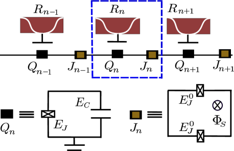
The principal building blocks of the envisioned simulator (for a schematic illustration, see Fig. 1 below) are SC transmon qubits () with the energy splitting , microwave resonators () with the photon frequency (assumed to be realized in the the form of coplanar waveguides Poz ), and SQUID loops (), each of which comprises two Josephson junctions with the energy (). The pseudospin- degree of freedom of the -th qubit will hereafter be represented by the Pauli operators . At the same time, microwave photons in the resonators, created (annihilated) by the operators (), play the role of dispersionless (Einstein-type) phonons.
The total Hamiltonian of the envisioned simulator can be written in the form
| (1) |
where accounts for the -th qubit, its corresponding resonator, and their mutual (qubit-resonator) always-on coupling, describes external microwave driving of the -th resonator, while describes the coupling between qubits and through the SQUID loop .
Here is given by a Hamiltonian of the Jaynes-Cummings form Jay :
| (2) |
While the first two terms on the right-hand-side (RHS) of the last equation describe the -th qubit and its corresponding resonator, respectively, the final term accounts for the capacitive qubit-resonator coupling SCq ; in particular, is the qubit-resonator coupling strength. At the same time, the resonators are driven by an ac microwave source described by the time-dependent Hamiltonian
| (3) |
where is the driving amplitude and its corresponding frequency.
The Hamiltonian , which describes the coupling between adjacent qubits and , can be written as
| (4) |
where is the gauge-invariant phase of the SC island of the -th qubit and the effective Josephson energy of the SQUID loop. In the regime of interest for transmon qubits (, where and are the Josephson- and charging energies of a single qubit, respectively), the term is well-approximated by an expansion up to the second order in , where this expansion involves (where is the quantum displacement of the gauge-invariant phase variables Gir ) as the relevant small parameter (for a typical transmon ); higher-order terms in that expansion, i.e. higher powers of the phase difference , can safely be neglected owing to their rapidly decaying prefactors, which are proportional to higher powers of . In this manner, upon switching to the pseudospin- (qubit) operators , the Hamiltonian in Eq. (4) can approximately be rewritten in the form (for a detailed derivation, see Ref. Nau )
| (5) |
where constant terms – immaterial for our present purposes – have been dropped. Assuming that every Josephson junction in the SQUID loops has the same energy and that an external magnetic flux of magnitude is threading each loop (cf. Fig. 1), the effective (-dependent) Josephson energy of a loop is given by Makhlin et al. (2001)
| (6) |
where is the magnetic-flux quantum.
It is important to point out that in the derivation of Eq. (5) the terms of the form and have been dropped. While this is permitted on the grounds of the rotating-wave approximation (RWA) – even in the most rigorous (multilevel) treatment of transmon qubits – in the problem under consideration there is an additional argument for neglecting such terms. Namely, in the single-excitation problem under consideration (see Sec. III.2 below) the relevant part of the total Hilbert space of the system comprises states with a single spinless fermion – which in the pseudospin- (qubit) representation correspond to states with exactly one qubit in the logical state (i.e. these states correspond to Hamming-weight- bit strings) – and the terms of the type and yield zero when acting on an arbitrary such state.
It is also worthwhile to note that the terms in Eq. (5) are of the same form as the single-qubit terms in [cf. (2)]; in other words, this type of qubit-resonator coupling leads to a shift in the qubit frequency. Therefore, it is pertinent to hereafter absorb this shift into the coefficients in front of the single-qubit terms in Eq. (2). The total Hamiltonian of the analog simulator under consideration [cf. Eq. (1)] is then given by [cf. Eqs. (2) - (5)]
| (7) |
The last term on the RHS of this equation, with the prefactor , describes the -type (flip-flop) coupling between adjacent transmon qubits.
III Effective Holstein-like Hamiltonian
In the following, the effective Hamiltonian of the envisioned analog simulator in the dispersive regime of circuit QED is first derived (Sec. III.1). This is followed by the identification of this effective model with the Holstein Hamiltonian via the Jordan-Wigner transformation Col and a discussion of the relevant parameter regimes (Sec. III.2).
III.1 Derivation of the effective system Hamiltonian
The proposed simulator is meant to operate in the dispersive regime of circuit QED , which is defined by the condition that the detuning between the resonator and qubit frequencies is much larger than the qubit-resonator coupling strength , i.e. .
The standard practice in the treatment of the Jaynes-Cummings model [cf. Eq. (2)] and some of its generalizations in the dispersive regime, is to first apply a Schrieffer-Wolff-type canonical transformation Kli , defined by a certain generator (i.e. ), such that the term linear in the light-matter coupling completely vanishes. One such generalization is the quantum Rabi model Rab ; Wal ; Ric , which – unlike the Jaynes-Cummings model itself – also includes the off-resonant qubit-photon interaction processes (i.e. the counter-rotating terms and ), so that the resulting qubit-resonator interaction assumes the form (the so-called transverse coupling term Ric ). In particular, in the case of the Jaynes-Cummings model the desired canonical-transformation generator is given by Boi ; Hau
| (8) |
In the following, with the aim of obtaining an effective Holstein-type Hamiltonian of the envisioned analog sumulator, this same canonical transformation will be applied to the total Hamiltonian of the system [cf. Eq. (7)]. This transformation will be carried out by making use of the well-known operator identity
| (9) |
where the ellipses on the RHS of the last equation denote higher-order repeated commutators of the operators and . More specifically yet, the Hamiltonian will be obtained by keeping only the leading-order terms in the small parameter .
By carrying out the canonical transformation with the generator given by Eq. (8), the Jaynes-Cummings contribution to the total system Hamiltonian is transformed into the Hamiltonian . The latter is given by
| (10) |
where is the Stark shift . The last term on the RHS of Eq. (10) effectively renders the transition frequency of the resonator dependent on the state of the qubit and vice versa . The very existence of this term demonstrates that qubits and resonators are inevitably getting entangled through their always-on interaction.
One can derive and in a similar fashion, obtaining as a result the transformed total Hamiltonian . It is pertinent to analyze this transformed Hamiltonian in the interaction picture – i.e. the rotating frame – defined by the Hamiltonian
| (11) |
where is the modified detuning of the resonator frequency from that of the external driving and the modified qubit frequency. To this end, it is useful to recall that in the rotating frame defined by a time-independent Hamiltonian the (rotating-frame) counterpart of a general Hamiltonian is given by SCq
| (12) |
where is the Hermitian adjoint of the time-evolution operator corresponding to .
By means of the RWA, i.e. disregarding rapidly-rotating terms such as , one finds that the counterpart of the transformed [by the above Schrieffer-Wolff-type canonical transformation; cf. Eq. (8)] total Hamiltonian of the system in the interaction picture (i.e., in the rotating frame defined by the Hamiltonian ) is given by
| (13) |
where the Hamiltonian assumes the form
| (14) |
and is given by Eq. (5).
The next step in the derivation of an effective Hamiltonian of the envisioned SC analog simulator is to apply a unitary transformation based on the Glauber’s displacement operator , with , in order to shift the resonator modes according to [recall that, in general, ] Wal . The resulting Hamiltonian [obtained from the one in Eq. (13)] assumes the form of an interacting qubit-resonator (i.e. qubit-photon) Hamiltonian
| (15) | |||||
where and in the last derivation it was assumed that .
III.2 Holstein-like effective Hamiltonian and the relevant parameter regime
The final step in deriving an effective Holstein-like Hamiltonian of the system at hand entails switching from the pseudospin- operators representing qubits to the operators () representing spinless fermions by making use of the Jordan-Wigner transformation Col :
| (16) |
On account of the fact that this last transformation maps into the spinless-fermion hopping term , the Hamiltonian of Eq. (15) can finally be recast in the form
| (17) | |||||
characteristic of the Holstein model with a single itinerant spinless-fermion excitation locally coupled to dispersionless phonons (here emulated by photons in the resonators). Here , explicitly given by [cf. Eq. (6)]
| (18) |
is the in-situ flux-tunable (nearest-neighbor) hopping amplitude of a spinless-fermion excitation, and
| (19) |
the resulting dimensionless Holstein-type (local) e-ph coupling strength; the role of the effective phonon frequency is played by .
Before embarking on the discussion as to which regimes of the Holstein model are realizable in the analog simulator at hand, it is useful to start with some general considerations. The effective e-ph coupling strength in a -dimensional Holstein model with the excitation hopping amplitude , the phonon frequency , and the dimensionless coupling strength is given by the ratio of the polaron binding energy in the strong-coupling regime and the average bare-excitation kinetic energy (equal to the half of the bare-excitation bandwidth) , i.e., Alexandrov and Devreese (2010)
| (20) |
The criterion for the formation of small Holstein polarons is that the conditions and are simultaneously satisfied Alexandrov and Devreese (2010). In the adiabatic regime (), the condition is more difficult to satisfy – hence being more restrictive – than . On the other hand, becomes the more restrictive of the two conditions in the antiadiabatic regime ().
Based on the general expression in Eq. (20), the effective Holstein e-ph coupling strength in the one-dimensional () system at hand (where the role of is played by ) is given by
| (21) |
This effective coupling strength will be varied in the following by exploiting its dependence on the hopping amplitude ; importantly, itself can be varied by exploiting its dependence on the external flux [cf. Eq. (18)]). By combining Eqs. 19 and 21, one obtains the explicit expression for as a function of the system parameters:
| (22) |
It is pertinent to consider at this point a choice of parameter values that allows one to realize the relevant regimes of the Holstein model within the framework of the envisioned analog simulator. Firstly, for the qubit-resonator coupling strength in a typical circuit-QED setup one has MHz . Secondly, the envisioned simulator will be assumed to operate in the regime of weak drives, i.e. for . For instance, MHz is one value of the driving amplitude that satisfies this constraint. The detuning will be assumed to have the value GHz, which – along with the aforementioned value of – clearly satisfies the condition that defines the dispersive regime of circuit QED [recall Sec. III.1]; the corresponding value of the Stark shift is MHz. Finally, the value MHz will be used for the parameter .
By inserting the chosen parameter values into Eq. (19) above, it is straightforward to obtain the value for the dimensionless e-ph coupling strength in the system at hand. From this last value for , which is kept fixed throughout the following discussion, different values of the effective coupling strength can be obtained from Eq. (21) by varying the effective hopping amplitude (or, equivalently, by changing the adiabaticity ratio ). This is physically achieved by varying the external flux through the SQUID loops (cf. Fig. 1), which determines the value of [cf. Eq. (18)]; therefore, the flux is the main experimental knob in the system at hand. Importantly, for the chosen values of the relevant system parameters one of the two conditions for the existence of small Holstein polarons (namely, ) will always be fulfilled, while the other one () will be satisfied for sufficiently large values of the adiabaticity ratio (more precisely, for ).
IV Spectral function: Definition, measurement, and evaluation
In the following, after some preliminary considerations of the implications of the discrete translational symmetry in the coupled e-ph system at hand (Sec. IV.1), the most important general properties of the momentum-frequency resolved spectral function are briefly reviewed (Sec. IV.2). It is then explained how this dynamical response function can be experimentally extracted in the envisioned analog simulator (Sec. IV.3). Finally, the relevant details of the evaluation of this spectral function using the KPM are described (Sec. IV.4).
IV.1 Implications of discrete translational symmetry
Direct implications of the discrete translational symmetry of the problem at hand are discussed in the following, starting with the momentum-space form of the total Hamiltonian of the system. Importantly, in what follows all quasimomenta will be expressed in units of the inverse lattice spacing, thus the Brillouin zone of the system corresponds to .
The momentum-space form of total Hamiltonian of the system is given by , where
| (23) |
is the noninteracting part, with being the (one-dimensional) tight-binding dispersion of an itinerant spinless-fermion excitation and the frequency of zero-dimensional phonons. The interacting (e-ph) part assumes the generic form
| (24) |
where is the e-ph vertex function. In the special case of the Holstein model, the corresponding vertex function is completely independent of and , more precisely .
Regardless of the concrete form of the e-ph vertex function, by virtue of the discrete translational symmetry of the system, its total Hamiltonian ought to commute with the total quasimomentum operator
| (25) |
Because , the (phonon-dressed) Bloch eigenstates of are also the eigenstates of (instead of being eigenstates of , as would be the case in the absence of e-ph coupling). In other words, the total Hamiltonian of the system can be diagonalized in sectors of the total e-ph Hilbert space that correspond to the eigensubspaces of . For each eigenvalue of , the Bloch eigenstates of the coupled e-ph system [in the system at hand described by the Hamiltonian in Eq. (17)] form a complete set of states within the corresponding sector of the Hilbert space of the coupled e-ph system.
The fact that the coupled e-ph system at hand has a discrete translational symmetry enables one to introduce a symmetry-adapted basis [cf. Appendix A]. The use of this basis allows one to perform the evaluation of the spectral properties more efficiently than in a generic basis.
IV.2 Momentum-frequency resolved spectral function
The established framework for characterizing excitations in many-body systems is based on the use of dynamical response functions Foe . The latter are defined through Fourier transforms of retarded two-time correlation functions, an important example being furnished by the single-particle retarded Green’s function.
The single-particle retarded Green’s function is employed to, e.g., describe the propagation of a single electron (or a hole) in solid-state systems. In the problem under consideration, this Green’s function will be used for the description of an itinerant spinless-fermion excitation coupled with zero-dimensional (dispersionless) bosons residing on sites of a one-dimensional lattice.
In the problem at hand, the relevant single-particle retarded Green’s function is defined as
| (26) |
where is a single-particle creation operator in the Heisenberg representation [with being the time-evolution operator corresponding to the governing Hamiltonian of the system] and the ground state of the system; is the Heaviside function and stands for an anticommutator of two operators.
The single-particle retarded Green’s function describes the linear response of the system to the addition of a single fermion. Its Fourier transform can formally be evaluated provided that a regularization factor is included (), i.e.,
| (27) |
By evaluating the last Fourier transform with the expression for from Eq. (26), one obtains
| (28) | |||||
where is the ground-state energy of the system.
The momentum-frequency resolved spectral function, the dynamical response function of interest in the problem at hand, is given by the imaginary part of :
| (29) |
By making use of the special case
| (30) |
of the Sokhotski-Plemelj theorem, where and stands for the principal part, along with the fact that the Bloch eigenstates of the total coupled e-ph Hamiltonian form a complete set of states, one can explicitly express the spectral function in terms of the eigenstates and eigenvalues of . More precisely, is given by
| (31) |
where is the energy eigenvalue corresponding to the eigenstate .
In connection with the relevant single-particle spectral function in the problem at hand [cf. Eq. (29)], which corresponds to adding a single fermion to the vacuum, a remark is in order here. It is important to first note that in the solid-state-physics context (i.e. in real electronic materials) the more relevant single-particle spectral function is the so-called electron-removal spectral function [denoted by ], as the latter can be experimentally measured using angle-resolved photoemission spectroscopy (ARPES) Dam . However, after a removal of an itinerant fermionic (e.g. electronic) excitation in a system that only involves dispersionless (Einstein-type) phonons – as is the case for the Holstein model investigated here – the phonon degrees of freedom remain frozen and there is no dynamics left in the system. This also explains why not much attention has heretofore been devoted to the electron-removal spectral function of the Holstein model; this last spectral function is physically meaningful only for a generalized version of the Holstein model that involves phonons with dispersion Bon . To summarize, in the Holstein-polaron problem under consideration, only the spectral function [cf. Eq. (29)] makes sense physically.
For the sake of completeness, it is worthwhile to mention the intimate connection between the spectral function of a coupled e-ph system and its nonequilibrium dynamics following an e-ph interaction quench. To be more precise, assuming that the initial state of an e-ph system is a bare-excitation Bloch state with quasimomentum , the spectral function is equal to the Fourier transform of the matrix element , where is the state of the coupled e-ph system at time ; this state is given by a linear combination of Bloch states of the phonon-dressed excitation with the same total quasimomentum . The module squared of this matrix element – i.e. the survival probability of the initial bare-excitation Bloch state with quasimomentum – is a special case of the quantity that is known as the Loschmidt echo.
In the envisioned analog simulator that consists of qubits, the bare-excitation Bloch state – when recast in terms of pseudospin- (qubit) degrees of freedom via the Jordan-Wigner transformation [cf. Eq. (III.2)] – corresponds to a generalized (twisted) -qubit state Haa ; in particular, the state corresponds to an ordinary -qubit state Sto (a); Zha (c).
IV.3 Measurement of the spectral function in the superconducting analog simulator
Having reviewed the general properties of the momentum-frequency resolved spectral function in Sec. IV.2, it is pertinent to discuss at this point some relevant aspects in the proposed SC analog simulator.
To begin with, it is worthwhile noting that – while the anticommutator retarded Green’s function, defined in Eq. (26), is the appropriate choice for spinless-fermion excitations discussed here – its commutator counterpart
| (32) |
has essentially the same physical content in the problem at hand. Namely, given that is a vacuum state, one has , which readily implies that in the single-particle problem under consideration the two retarded Green’s functions differ only by their sign, i.e., . Therefore, provided that there is a way to determine the retarded commutator Green’s function in the proposed analog simulator, its anticommutator counterpart is also recovered.
Importantly, can experimentally be determined in the envisioned simulator using a previously proposed scheme based on the many-body version of the Ramsey interference protocol Knap et al. (2013); a special case of this scheme, adapted for systems of the type considered here, is briefly reviewed in Appendix B. More precisely, that scheme allows one to extract the real-space retarded (commutator) Green’s functions
| (33) |
which in systems with a discrete translational symmetry depend only on , by measuring a set of retarded two-time correlation functions defined in terms of pseudospin- operators (for details, see Appendix B). Once is obtained in this manner, the retarded momentum-space Green’s function can be determined (for different quasimomenta ) through a spatial Fourier transformation; for the reasons stated above, this immediately also yields . Finally, once is obtained at different times , using a numerical Fourier transform to the frequency domain the spectral function can be evaluated for a broad range of frequencies based on Eq. (29).
IV.4 Numerical evaluation of the spectral function using the KPM
In this work the KPM (for a brief review of its basic aspects, see Appendix C) is employed to compute the momentum-frequency resolved spectral function [cf. Eq. (29)]. The relevant details of the KPM-based evaluation of this spectral function are described in what follows.
As a preparatory step for the evaluation of using the KPM, the spectrum of the total effective Hamiltonian of the e-ph system at hand has to be mapped to the domain of Chebyshev polynomials of the first kind Wei . This is done by introducing the Hamiltonian
| (34) |
which is shifted and rescaled with respect to . Here and are the largest and smallest eigenvalue of , respectively, which can both be obtained using the Lanczos algorithm Cullum and Willoughby (1985). Finally, is an auxiliary parameter that allows one to avoid stability problems at the boundaries of the spectrum; the value will be used in what follows.
By inserting into the expression for the spectral function [cf. Eq. (31)], one readily obtains
| (35) | |||||
where are the eigenvalues of and
| (36) |
is a shifted and rescaled frequency. Equation (35) can be recast more succinctly as
| (37) |
where is an auxiliary function, defined as
| (38) |
In this last expression, can be expanded into a series of polynomials and approximated by with a large order [cf. Eq. (66)].
Using the general definition of Eq. (65), the Chebyshev moments corresponding to can be shown to be of the form
| (39) |
In order to efficiently compute , one makes use of the well-known recurrence relation for Chebyshev polynomials of the first kind Shi :
| (40) |
In view of this recurrence relation, it is pertinent to define the states and , as well as
| (41) |
for .
It is worthwhile to note that the states in Eq. (41) naturally occur when applying the above recurrence relation to Eq. (39). Furthermore, their use renders the evaluation of the Chebyshev moments by iteration rather straightforward. More precisely, starting from and , one obtains the following expressions:
| (42) |
While already the form of Eq. (41) indicates that the matrix-vector multiplication (MVM) is the essential operation for the implementation of the KPM Wei , the last equation implies that in the problem at hand one can compute two moments from every new state . In other words, two new moments can be obtained by carying out a single MVM.
The described computational scheme allows a resource-efficient evaluation of the spectral function, given that – being subject to Eq. (41) – only three states have to be stored at each step of the evaluation. This is in stark contrast with the Lanczos recursion methods Cullum and Willoughby (1985), where a similar iteration has to be performed, but with a simultaneous preservation of orthogonality at each step. Because of that, the KPM is faster and less memory-consuming than the Lanczos methods. Another important advantage of the KPM compared with the latter methods is that it avoids accumulation of numerical roundoff errors even in cases where it entails large numbers of MVMs Sil (b).
The final step in the evaluation of entails – in the interest of achieving a high numerical efficiency – a special choice of values for the rescaled frequency, namely
| (43) |
By inserting these last special frequency values into Eq. (66) and making use of the identity for , one arrives the following result for :
| (44) | |||||
It is worthwhile noting that this last expression amounts to a discrete Fourier transformation, which – as usual – can be executed with a relatively modest computational effort [namely, with operations] using the fast-Fourier-transform (FFT) algorithm NRc .
With evaluated in the aforementioned fashion, the final step in computing the spectral function entails inserting the last result for [cf. Eq. (44)] into
| (45) |
an approximated form of Eq. (37), where
| (46) |
are the shifted and rescaled energy values [cf. Eq. (36)]. Importantly, while there are different possible choices of attentuation factors in Eq. (44) – hence also in Eq. (45) – it was demonstrated that those originating from the Jackson kernel [cf. Eq. (70)] are the optimal choice for evaluating spectral functions using the KPM Sil (b).
It is important to stress that the achievable energy resolution in evaluating spectral functions of the type discussed here using the KPM is inversely proportional to the number of Chebyshev moments used. For a chosen energy resolution, the memory required for Hamiltonians represented by sparse matrices can scale linearly in the number of states Sil (b).
V Results and Discussion
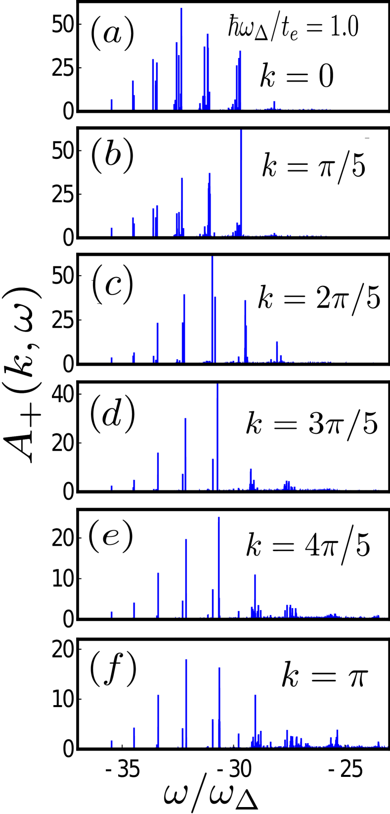
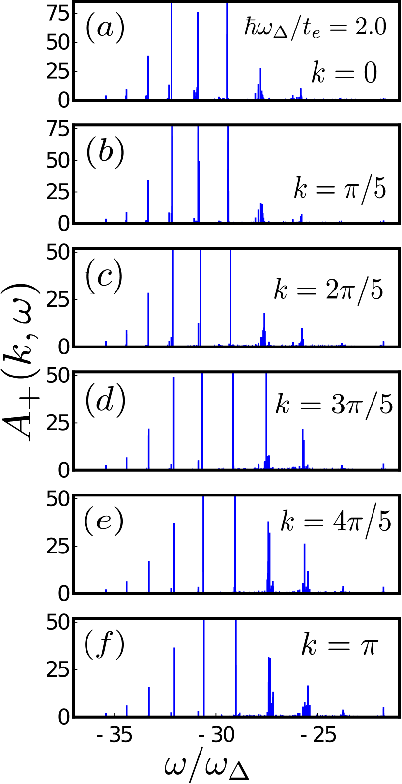
In what follows, the results for the momentum-frequency resolved spectral function [cf. Eq. (31)] inherent to the Holstein model, obtained using the KPM (for the basic aspects of this method, see Appendix C) are presented. All the results to be discussed in the following correspond to a system with sites and up to phonons in the truncated phonon Hilbert space; the dimension of this space is (a controlled truncation of the Hilbert space of a coupled e-ph system is discussed in Appendix A). To achieve a sufficiently good spectral resolution, as many as Chebyshev moments were evaluated and used in the expansion of the spectral function (cf. Sec. IV.4).
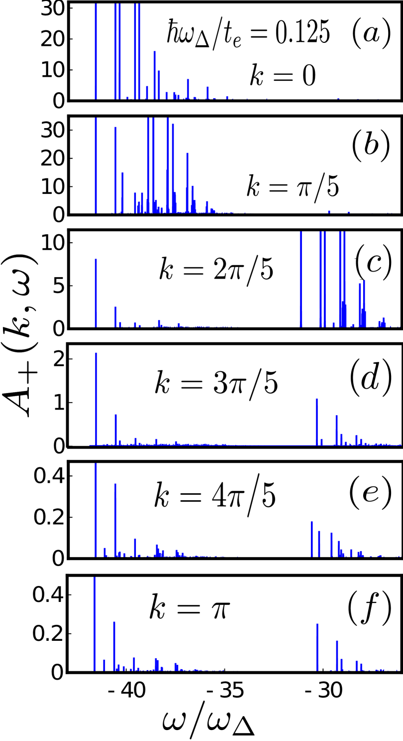
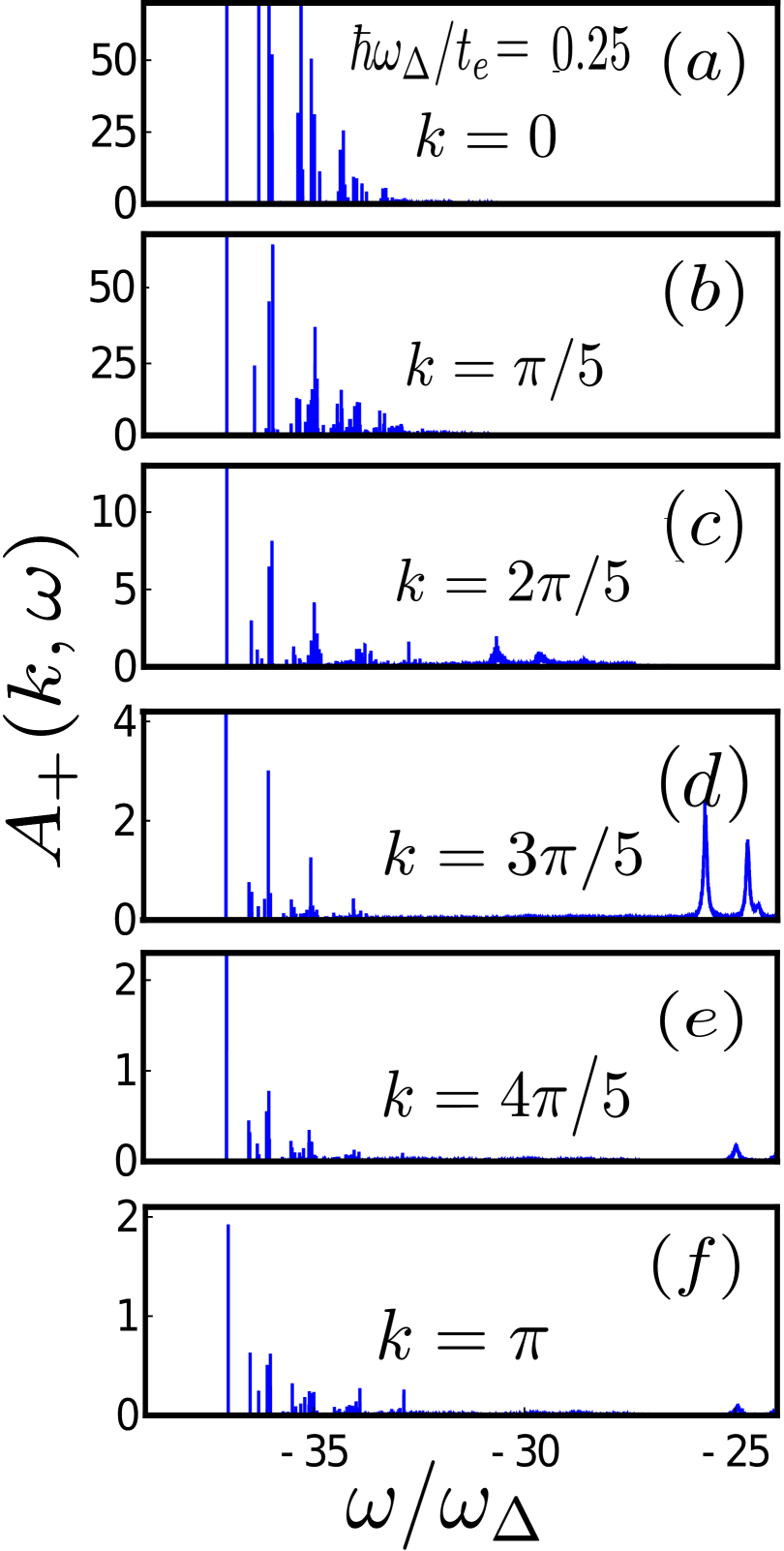
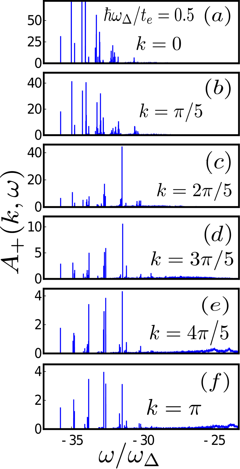
The single-particle spectral function is evaluated in the following for five different values of the adiabaticity ratio (cf. Sec. III.2), namely . For and the corresponding effective coupling strengths are and , respectively; in those cases , thus the second condition for the formation of small Holstein polarons is not fulfilled. For the remaining three values of , the system at hand is in the small Holstein-polaron regime (, ).
The coupled e-ph system at hand is treated in what follows under the assumption of periodic boundary conditions (PBC). Generally speaking, in a system defined on a discrete lattice with sites, the PBC imply that there are exactly permissible quasimomenta in the Brillouin zone; they are given by , where ( is assumed to be even). In the system under consideration, with , those quasimomenta are . For each choice of the relevant parameters, the frequency dependence of the spectral function is presented in what follows for six different quasimomenta in the positive half of the 1D Brillouin zone of the system (namely, for ), consistent with the PBC.
The numerical evaluation of the single-particle spectral function using the KPM was performed on a -core, GHz AMD Ryzen Threadripper PRO 5995WX workstation, with the main memory of GB; the computational runs required to obtain all the results presented in this section took in total about hours. Those results for the spectral function are depicted in Figs. 2 - 6 below.
To make the interpretation of the obtained results more straightforward, it is pertinent to reiterate some of the generic properties of the energy spectra of models describing a short-range coupling of an itinerant excitation with Einstein-type (zero-dimensional) phonons; the Holstein model, considered in this paper, represents the extreme realization of such models in that the Holstein-type e-ph coupling is completely local in real space. In the strong-coupling regimes of such models, heavily-dressed excitations (small polarons) are formed. Irrespective of the concrete form of the e-ph coupling in such a model, the center of the small-polaron Bloch band is shifted by an energy (the small-polaron binding energy) below that of a bare-excitation band.
For each fixed quasimentum , the eigenstates of a coupled e-ph problem that contribute to the spectral function [cf. Eq. (31)] include the discrete states (i.e. those belonging to coherent Bloch bands of a phonon-dressed excitation) and their corresponding continua. In particular, the energetic width of each of those continua equals the width of of the respective polaron Bloch band. Importantly, the one-phonon continuum corresponds to the inelastic-scattering threshold, i.e. the minimal energy that a phonon-dressed excitation must have to be capable of emitting a phonon. The one-phonon continuum sets in at the single-phonon energy (where is the relevant phonon frequency) above the ground-state energy of the coupled e-ph system Engelsberg and Schrieffer (1963) [recall that in the system under consideration the role of the effective phonon freqency is played by (cf. Sec. III.1)]. In the weak e-ph coupling regime of the Holstein- and similar models, a coupled e-ph system only has one discrete Bloch state at quasimomentum – which in the case represents the ground state of the coupled e-ph system – and its corresponding continuum of states corresponds to a phonon-dressed excitation with quasimomentum and an unbound phonon with quasimomentum . Because such a state exists for all possible phonon momenta in the Brillouin zone, in the presence of dispersionless phonons the energetic width of this continuum is equal to the width of the dressed-excitation Bloch band.
In the weak-coupling regime, the spectrum of a phonon-dressed excitation is virtually unaffected by the presence of e-ph coupling for energies below the phonon-emission threshold. Consequently, in the weak-coupling adiabatic regime (), the phonon-renormalised dispersion of a spinless-fermion excitation mimics the tight-binding cosine dispersion of a bare excitation up to a certain quasimomentum that corresponds to the energy from the bottom of the band. For quasimomenta above , spinless-fermion- and phonon states start to hybridise, which leads to the band-flattening phenomenon Feh .
For larger e-ph coupling strengths, additional coherent polaron bands [i.e., additional discrete (split off from the continuum) states at each quasimomentum in the Brillouin zone of the relevant system] begin to emerge. The first such excited dressed-excitation (in the extreme case small-polaron-) state at quasimomentum pertains to a phonon-dressed excitation bound with an additional phonon, such that the total quasimomentum is distributed between the phonon-dressed excitation (quasimomentum ) and the additional phonon (quasimomentum ). As e-ph coupling strength continues to increase, another (second) excited state, representing a bound state of a polaron and two additional phonons (with the same total quasimomentum ) sets in. All those discrete states, together with their respective continua – separated from them by the energy of a single phonon – provide additional contributions to the spectral function at the quasimentum Feh .
In accordance with general characteristics of the energy spectra of (short-range) coupled e-ph Hamiltonians, for increasing values of the adiabaticity ratio , which in the system at hand translate into larger values of the effective e-ph coupling strength [cf. Eq. (21)], one can notice an increasing number of discrete peaks in the single-particle spectral function. In particular, for the Holstein model it is known that at the onset of the strong-cupling regime there are three such peaks. In the system under consideration, from Figs. 5 and 6 it can be inferred that for the largest effective coupling strength considered ( and , respectively, which both belong to the deep strong-coupling regime) there are up to six such peaks, accompanied by their respective continua.
VI Summary and Conclusions
In this paper it was demonstrated how spectral properties of small Holstein polarons can be investigated using an analog superconducting quantum simulator that consists of capacitively-coupled transmon qubits and microwave resonators, the latter being subject to a weak external driving field. It was shown here that the envisioned analog simulator, operating in the dispersive regime of circuit quantum electrodynamics, allows one to access all the relevant physical regimes of the Holstein model. Using the kernel-polynomial method the relevant single-particle momentum-frequency resolved spectral function of this system was computed here for a broad range of values for its characteristic parameters. Finally, to make contact with anticipated experimental realizations, it was also demonstrated that – by employing the many-body version of the Ramsey interference protocol – this important dynamical-response function can be extracted experimentally in the proposed analog simulator.
The present study complements investigations of electron-phonon coupling effects in solid-state systems in two important respects. Firstly, it allows a nearly-ideal physical realization of the pristine Holstein model with purely dispersionless (Einstein-type) phonons, the latter being an idealization for optical phonons in solid-state materials. Secondly, it presents results for a specific type of single-particle spectral functions (namely, the one corresponding to the addition of a single itinerant excitation to the vacuum state) that cannot be directly measured using conventional methods of experimental solid-state physics (such as ARPES), proposing also a scheme for the measurement thereof in locally-addressable analog simulators.
The scheme proposed in this paper can be generalized to other physical realizations of the Holstein model, i.e. to its analog simulators based on different physical platforms, for example with trapped ions in arrays of microtraps. Moreover, recent developments in the field of superconducting qubits Wen ; Gu+ ; SCq ; SCd ; SCc should make it possible to engineer qubit arrays of more nontrivial geometry, that could mimic the geometries inherent to complex electronic materials Van . Finally, analog simulators that display similar functionalities as transmon-based ones can be engineered using other types of superconducting qubits. For example, models akin to the Holstein model Roo can also be emulated with arrays of flux qubits Vol ; Fis and their spectral properties investigated based on the general strategy that was laid out here. Experimental realizations of the envisioned superconducting analog simulator and the proposed method for extracting the spectral properties of small Holstein polarons is keenly anticipated.
Acknowledgements.
The author acknowledges useful discussions on the numerical implementation of the kernel polynomial method with J. K. Nauth. This research was supported by the Deutsche Forschungsgemeinschaft (DFG) – SFB 1119 – 236615297.Appendix A Truncated Hilbert space and its symmetry-adapted basis
The infinite-dimensional character of the phonon (or, more generally, boson) Hilbert spaces requires one to carry out a controlled truncation of the Hilbert space of the coupled e-ph system under consideration. In the following, the essential details of this Hilbert-space truncation are discussed, along with the introduction of the basis adapted to the discrete translational symmetry of the system at hand (the symmetry-adapted basis).
The Hilbert space of the coupled e-ph system under consideration, defined on a lattice with sites, is spanned by states , where corresponds to the excitation at the site and
| (47) |
with being the set of phonon occupation numbers at different lattice sites.
In view of the infinite-dimensional phonon Hilbert spaces, one ought to restrict oneself to the truncated phonon Hilbert space that consists of states whose corresponding total phonon number is not larger than , where . Consequently, the total Hilbert space of the coupled e-ph system has the dimension , where for a lattice with sites and .
It is important to stress that the choice of the maximal total number of phonons, which determines the total dimension of the Hilbert space of a coupled e-ph system, is governed by the required numerical accuracy in evaluating the desired physical observables (e.g. the ground-state energy, expected total phonon number in the ground state, quasiparticle spectral weight, etc.). The aforementoned controlled truncation of the Hilbert space of a coupled e-ph system is carried out by gradually increasing the number of sites , and subsequent increase in the total number of phonons , up to the point where their further increase does not lead to an appreciable change (in accordance with the accepted error margin) in the obtained results for the physical observables of interest.
The dimension of the matrix-diagonalization problem for the total Hamiltonian of the system can further be reduced by taking advantage of the discrete translational symmetry of the system, mathematically expressed as the commutation of operators and . This allows one to diagonalize in Hilbert-space sectors corresponding to the eigensubspaces of . The dimension of each of those -sectors of the total Hilbert space is equal to the dimension of the truncated phonon Hilbert space (i.e., ). Therefore, it is pertinent to utilize the symmetry-adapted basis
| (48) |
where () are the (discrete) translation operators, whose action complies with the PBC. Equation (48) can be rewritten in the form
| (49) |
with the discrete-translation operators acting on the phonon Hilbert space.
In particular, if is given by a set of occupation numbers
| (50) |
then the -th occupation number corresponding to the state is given by , where is defined as
| (51) |
Appendix B Measurement of via many-body Ramsey protocol
In the following, we recapitulate essential elements of the method for the experimental measurement of retarded Green’s functions using the many-body (multiqubit) version of the Ramsey interference protocol Knap et al. (2013), which in Ref. Stojanović et al. (2014) was adapted to systems of the type discussed in the present work.
The real-space retarded (commutator) Green’s functions
| (52) |
which in systems with a discrete translational symmetry depend only on , are given by the spatial Fourier transform
| (53) |
of the momentum-space-resolved ones [cf. Eq. (32)]. They can straightforwardly be recast in terms of pseudospin- operators as Stojanović et al. (2014)
| (54) |
where the Jordan-Wigner transformation Col [for the explicit form of this transformation, see Eq. (III.2) above] allows one to switch from spinless-fermion- to the pseudospin- operators. It is straightforward to show that can be rewritten in the form Stojanović et al. (2014)
| (55) |
with the retarded pseudospin- two-time correlation functions ( ), which are defined as Stojanović et al. (2014)
| (56) |
[For the sake on simplicity, the superscript has been omitted in the notation for these last retarded two-time correlation functions; the same convention is used in the remainder of this section.]
The many-body version of the Ramsey interference protocol, which can be utilized in all systems that are addressable at the single-qubit level, yields the real-space- and time-resolved commutator Green’s functions of spin- (or pseudospin-) operators Knap et al. (2013). This protocol makes use a special type of Rabi pulses, which are written in the general form
| (57) |
Here – with being the Rabi frequency and the pulse duration – is the pulse area and the phase of the laser field. The effect of such pulses on, e.g., the spin-down (logical-zero) state of a single qubit is given by .
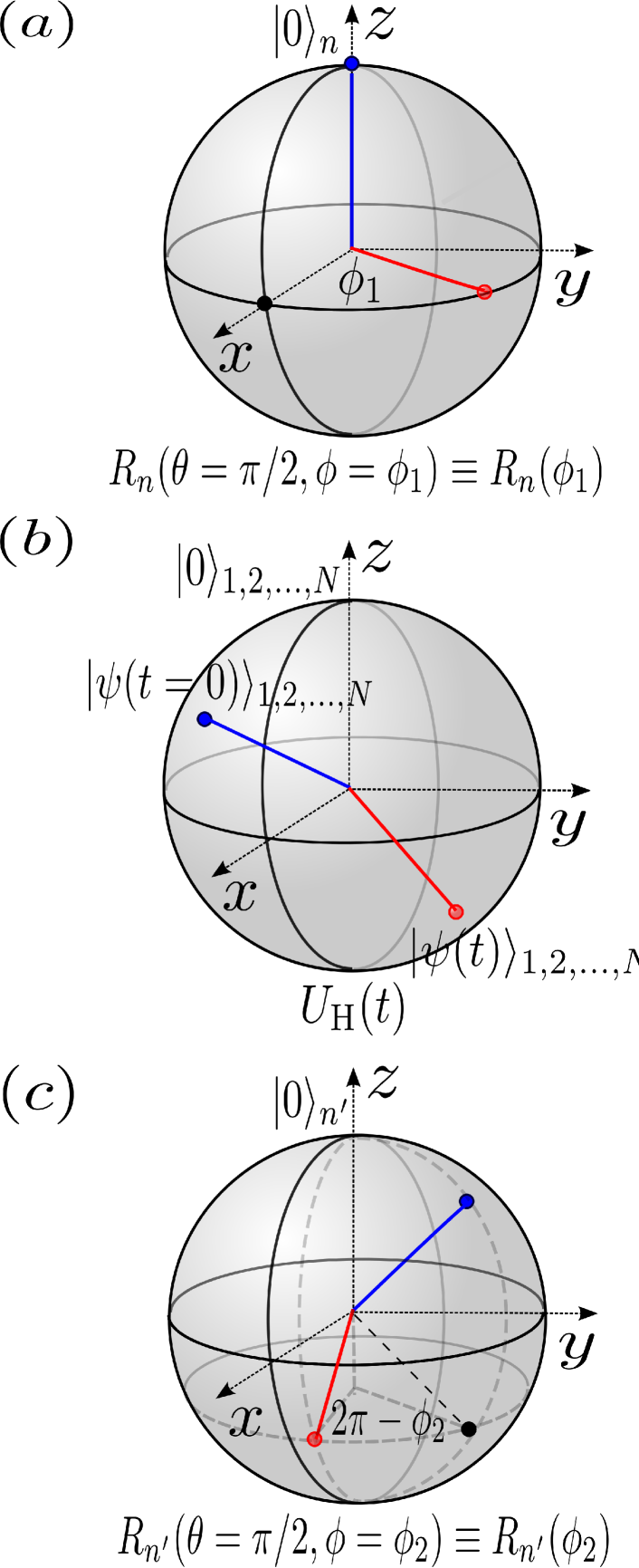
This generalized Ramsey-interference protocol consists of the following steps (for a pictorial illustration, see Fig. 7), akin to those used in other applications of the Ramsey sequence Dog : a local -rotation at site (with the value of the parameter ), an evolution of the system over the time interval of duration , followed by a local -rotation at site or global -rotation (with the value of the parameter ), and, finally, a measurement of (i.e. the -component of the pseudospin at site ). The result of the final measurement of is given by Knap et al. (2013)
| (58) |
where is the state obtained from by performing the first three steps (two -rotations and a time evolution of duration ) of the Ramsey interference protocol (cf. Fig. 7). In other words, the state is given by
| (59) |
In order to elucidate the specific form of the measurement result in Eq. (58), expressed in terms of the retarded correlation functions [cf. Eq. (56)], in the problem under consideration it is important to note that the Holstein Hamiltonian – written in terms of pseudospin- (qubit) operators in Eq. (15) – has the symmetry under pseudospin rotations around the axis and the one under reflections with respect to the same axis. It can straightforwardly be shown that for a system with these two symmetries the expression for the final measurement result in the Ramsey protocol [cf. Eq. (58)] reads as follows Stojanović et al. (2014):
| (60) |
In particular, the terms and that one needs in order to to determine [cf. Eq. (55)] are given by for and , respectively.
Appendix C Basics of the KPM
In what follows, the mathematical basis for the KPM Sil (c) is briefly recapitulated. The basic ideas pertaining to applications of this method for evaluating spectral functions are also sketched. A more detailed introduction into the KPM and its use in many-body physics can be found in Ref. Wei .
The KPM allows one to efficiently compute dynamical properties of quantum many-body systems, which are typically described by spectral functions
| (61) |
Here is the relevant observable, while is the ground state of a system described by the Hamiltonian . This quantity can be recast in the form
| (62) |
where is the ground-state energy of the system and the energy of the -th excited state (); is the -th energy eigenstate of the system. The derivation of the last expression relies on the completeness of the set of eigenstates of the Hamiltonian (i.e., the relation ) and the use of identity in Eq. (30).
It is pertinent to note that the momentum-frequency resolved spectral function [cf. Eqs. (29) and (31) in Sec. IV.2], is a special case () of the general spectral function defined in Eq. (61) above.
The mathematical foundation of the KPM pertains to the problem of approximating a real-valued function Riv , which is defined on the interval , by a finite series
| (63) |
where () are Chebyshev polynomials of the first kind whose orthogonality relation is given by Shi
| (64) |
The coefficients in the above expansion (Chebyshev moments) are given by
| (65) |
For a sufficiently smooth function the last series converges uniformly to on any closed sub-interval of that excludes the endpoints Wei .
If the function that one aims to approximate is not continuous, the finite series in Eq. (63) cannot converge uniformly. More precisely, this series fails to converge in the vicinity of points where the function is not continuously differentiable. Instead, the series displays rapid Gibbs oscillations, the amplitude of which does not decrease in the limit where the number of terms in the series becomes infinite (the Gibbs phenomenon) Shi . However, the problem arising from the Gibbs phenomenon is known to be soluble for Chebyshev-polynomial expansions. In that case, for a fixed number of terms in the expansion, a set of attenuation (Gibbs damping) factors () can be found, which depend implicitly on , such that the modified finite-series approximants
| (66) |
accurately reproduce the function under consideration. Rephrasing, the introduction of these attenuation factors damps out high-frequency oscillations and constitutes the essential ingredient of the KPM.
The last truncation of the infinite series to order , along with the attendant modification of the coefficients in the expansion [ ], is equivalent to the convolution of the function under consideration with a kernel of the form
| (67) |
where the function is defined as
| (68) |
In other words, one has
| (69) |
Importantly, each choice of attenuation factors corresponds to one specific choice of kernel. In the problem at hand, it is pertinent to utilize the attenuation factors derived from the Jackson kernel Jac , which are given by Sil (b)
| (70) | |||||
This kernel was demonstrated to be the optimal choice for the evaluation of spectral functions [cf. Eqs. (61) and (62)] using the KPM Sil (b).
References
- (1) D. Hangleiter, J. Carolan, and K. Thebault, Analogue Quantum Simulation: A New Instrument for Scientific Understanding (Springer, Cham, Germany, 2022).
- Georgescu et al. (2014) I. M. Georgescu, S. Ashhab, and F. Nori, Rev. Mod. Phys. 86, 153 (2014).
- Bloch et al. (2008) I. Bloch, J. Dalibard, and W. Zwerger, Rev. Mod. Phys. 80, 885 (2008).
- (4) For an up-to-date review of Rydberg-atom based platforms, see, e.g., M. Morgado and S. Whitlock, AVS Quantum Sci. 3, 023501 (2021).
- (5) For a recent review of trapped-ion based platforms, see, e.g., C. D. Bruzewicz, J. Chiaverini, R. McConnell, and J. M. Sage, Appl. Phys. Rev. 6, 021314 (2019).
- (6) For a review, see B. Gadway and B. Yan, J. Phys. B 49, 152002 (2016).
- (7) For a recent review on superconducting qubits, see G. Wendin, Rep. Prog. Phys. 80, 106001 (2017).
- (8) For a review see, X. Gu, A. Frisk Kockum, A. Miranowicz, Y.-X. Liu, and F. Nori, Phys. Rep. 718, 1 (2017).
- (9) For a comprehensive review, see P. Krantz, M. Kjaergaard, F. Yan, T. P. Orlando, S. Gustavsson, and W. D. Oliver, Appl. Phys. Rev. , 021318 (2019).
- (10) For an introduction into SC quantum devices, see Y. Y. Gao, M. A. Rol, S. Touzard, and C. Wang, PRX Quantum , 040202 (2021).
- (11) For a systematic introduction into SC circuits, see S. E. Rasmussen, K. S. Christensen, S. P. Pedersen, L. B. Kristensen, T. Bækkegaard, N. J. S. Loft, and N. T. Zinner, PRX Quantum , 040204 (2021).
- Hohenadler et al. (2012) M. Hohenadler, M. Aichhorn, L. Pollet, and S. Schmidt, Phys. Rev. A 85, 013810 (2012).
- Gangat et al. (2013) A. A. Gangat, I. P. McCulloch, and G. J. Milburn, Phys. Rev. X 3, 031009 (2013).
- Kapit (2013) E. Kapit, Phys. Rev. A 87, 062336 (2013).
- Mei et al. (2013) F. Mei, V. M. Stojanović, I. Siddiqi, and L. Tian, Phys. Rev. B 88, 224502 (2013).
- Egger and Wilhelm (2013) D. J. Egger and F. K. Wilhelm, Phys. Rev. Lett. 111, 163601 (2013).
- (17) G. S. Paraoanu, J. Low. Temp. Phys. 175, 633 (2014).
- Stojanović et al. (2014) V. M. Stojanović, M. Vanević, E. Demler, and L. Tian, Phys. Rev. B 89, 144508 (2014).
- (19) U. Las Heras, A. Mezzacapo, L. Lamata, S. Filipp, A. Wallraff, and E. Solano, Phys. Rev. Lett. 112, 200501 (2014).
- (20) J. Leppäkangas, J. Braumüller, M. Hauck, J.-M. Reiner, I. Schwenk, S. Zanker, L. Fritz, A. V. Ustinov, M. Weides, and M. Marthaler, Phys. Rev. A 97, 052321 (2018).
- Stojanović and Salom (2019) V. M. Stojanović and I. Salom, Phys. Rev. B 99, 134308 (2019).
- Sto (a) V. M. Stojanović, Phys. Rev. Lett. , 190504 (2020).
- (23) J. K. Nauth and V. M. Stojanović, Phys. Rev. B , 174306 (2023).
- Koch et al. (2007) J. Koch, T. M. Yu, J. Gambetta, A. A. Houck, D. I. Schuster, J. Majer, A. Blais, M. H. Devoret, S. M. Girvin, and R. J. Schoelkopf, Phys. Rev. A 76, 042319 (2007).
- Wallraff et al. (2004) A. Wallraff, D. I. Schuster, A. Blais, L. Frunzio, R.-S. Huang, J. Majer, S. Kumar, S. M. Girvin, and R. J. Schoelkopf1, Nature (London) 431, 162 (2004).
- (26) For a theoretical introduction into circuit QED, see S. M. Girvin, in Quantum Machines: Measurement and Control of Engineered Quantum Systems, edited by M. Devoret, Lecture Notes of the Les Houches Summer School, Vol. 96, (Oxford University Press, Oxford, UK, 2014).
- (27) For an introduction, see U. Vool and M. Devoret, Int. J. Circ. Theor. Appl. 45, 897 (2017).
- Holstein (1959) T. Holstein, Ann. Phys. (N.Y.) 8, 343 (1959).
- Alexandrov and Devreese (2010) A. S. Alexandrov and J. T. Devreese, Advances in Polaron Physics (Springer-Verlag, Berlin, 2010).
- Hannewald et al. (2004) K. Hannewald, V. M. Stojanović, J. M. T. Schellekens, P. A. Bobbert, G. Kresse, and J. Hafner, Phys. Rev. B 69, 075211 (2004).
- (31) K. Hannewald, V. M. Stojanović, and P. A. Bobbert, J. Phys.: Condens. Matter , ().
- Sto (b) V. M. Stojanović, P. A. Bobbert, and M. A. J. Michels, Phys. Status Solidi C , ().
- Rösch et al. (2005) O. Rösch, O. Gunnarsson, X. J. Zhou, T. Yoshida, T. Sasagawa, A. Fujimori, Z. Hussain, Z.-X. Shen, and S. Uchida, Phys. Rev. Lett. 95, 227002 (2005).
- Vuk (a) N. Vukmirović, V. M. Stojanović, and M. Vanević, Phys. Rev. B , (R) ().
- Stojanović et al. (2010) V. M. Stojanović, N. Vukmirović, and C. Bruder, Phys. Rev. B 82, 165410 (2010).
- Vuk (b) N. Vukmirović, C. Bruder, and V. M. Stojanović, Phys. Rev. Lett. , 126407 (2012).
- (37) I. A. Makarov, E. I. Shneyder, P. A. Kozlov, and S. G. Ovchinnikov, Phys. Rev. B , 155143 (2015).
- Shn (a) E. I. Shneyder, S. V. Nikolaev, M. V. Zotova, R. A. Kaldin, and S. G. Ovchinnikov, Phys. Rev. B , 235114 (2020).
- Shn (b) E. I. Shneyder, M. V. Zotova, S. V. Nikolaev, and S. G. Ovchinnikov, Phys. Rev. B , 155153 (2021).
- Stojanović et al. (2004) V. M. Stojanović, P. A. Bobbert, and M. A. J. Michels, Phys. Rev. B 69, 144302 (2004).
- Stojanović and Vanević (2008) V. M. Stojanović and M. Vanević, Phys. Rev. B 78, 214301 (2008).
- Sto (c) V. M. Stojanović, Phys. Rev. B , 134301 (2020).
- (43) C. Slezak, A. Macridin, G. A. Sawatzky, M. Jarrell, and T. A. Maier, Phys. Rev. B , ().
- Sto (d) V. M. Stojanović, Phys. Rev. A , 022410 (2021).
- Jeckelmann and White (1998) E. Jeckelmann and S. R. White, Phys. Rev. B 57, 6376 (1998).
- Bonča et al. (1999) J. Bonča, S. A. Trugman, and I. Batistić, Phys. Rev. B 60, 1633 (1999).
- Ku et al. (2002) L.-C. Ku, S. A. Trugman, and J. Bonča, Phys. Rev. B 65, 174306 (2002).
- Zha (a) S. Zhao, Z. Han, S. A. Kivelson, and I. Esterlis, Phys. Rev. B , 075142 (2023).
- (49) P. M. Dee, B. Cohen-Stead, S. Johnston, and P. J. Hirschfeld, Phys. Rev. B , 104503 (2023).
- (50) S. Li, Y. Tang, T. A. Maier, and S. Johnston, Phys. Rev. B 97, 195116 (2018).
- (51) F. Hébert, B. Xiao, V. G. Rousseau, R. T. Scalettar, and G. G. Batrouni, Phys. Rev. B 99, 075108 (2019).
- (52) M. Kang, S. W. Jung, W. J. Shin, Y. Sohn, S. H. Ryu, T. K. Kim, M. Hoesch, and K. S. Kim, Nat. Mater. , 676 (2018).
- (53) C. Franchini, M. Reticcioli, M. Setvin, and U. Diebold, Nat. Rev. Mater. , 560 (2021).
- Stojanović et al. (2012) V. M. Stojanović, T. Shi, C. Bruder, and J. I. Cirac, Phys. Rev. Lett. 109, 250501 (2012).
- (55) F. Herrera and R. V. Krems, Phys. Rev. A , 051401(R) (2011); F. Herrera, K. W. Madison, R. V. Krems, and M. Berciu, Phys. Rev. Lett. 110, 223002 (2013).
- (56) Z. Huang, A. D Somoza, C. Peng, J. Huang, M. Bo, C. Yao, J. Li, and G. Long, New J. Phys. , 12302 (2021).
- Sil (a) R. N. Silver and H. Röder, Int. J. Mod. Phys. C 5, 735 (1994).
- (58) For an extensive review, see A. Weiße, G. Wellein, A. Alvermann, and H. Fehske, Rev. Mod. Phys. , 275 (2006).
- Sil (b) R. N. Silver, H. Röder, A. F. Voter, and D. J. Kress, J. Comput. Phys. , 115 (1996).
- Sil (c) R. N. Silver and H. Röder, Phys. Rev. E 56, 4822 (1997).
- (61) A. Alvermann and H. Fehske, Phys. Rev. B , 045125 (2008).
- (62) G. Schubert, G. Wellein, A. Weisse, A. Alvermann and H. Fehske, Phys. Rev. B , 104304 (2005).
- (63) T. Jiang, J. Ren, and Z. Shuai, J. Phys. Chem. Lett. , 9344 (2021).
- (64) J. E. Sobczyk and A. Roggero, Phys. Rev. E , 055310 (2022).
- Zha (b) P.-Y. Zhao, K. Ding, and S. Yang, Phys. Rev. Res. , 023026 (2023).
- Knap et al. (2013) M. Knap, A. Kantian, T. Giamarchi, I. Bloch, M. D. Lukin, and E. Demler, Phys. Rev. Lett. 111, 147205 (2013).
- (67) D. M. Pozar, Microwave Engineering (John Wiley & Sons, Hoboken, New Jersey, 2012), 4th ed.
- (68) J. Larson and T. Mavrogordatos, The Jaynes-Cummings Model and Its Descendants, IOP Series on Quantum Technology (IOP ebooks, Bristol, UK, 2021).
- Makhlin et al. (2001) Y. Makhlin, G. Schön, and A. Shnirman, Rev. Mod. Phys. 73, 357 (2001).
- (70) See, e.g., P. Coleman, Introduction to Many-Body Physics (Cambridge University Press, Cambridge, UK, 2015).
- (71) See, e.g., A. B. Klimov, L. L. Sánchez-Soto, A. Navarro, and E. C. Yustas, J. Mod. Opt. 49, 2211 (2002).
- (72) I. I. Rabi, Phys. Rev. 51, 652 (1937).
- (73) For an introduction, see, e.g., D. F. Walls and G. J. Milburn, Quantum Optics, 2nd ed. (Springer, Berlin, 2008).
- (74) For an application of this model to superconducting qubits, see, e.g., S. Richer and D. P. DiVincenzo, Phys. Rev. B 93, 134501 (2016).
- (75) M. Boissonneault, J. M. Gambetta, and A. Blais, Phys. Rev. A 79, 013819 (2009).
- (76) J. Hausinger and M. Grifoni, Phys. Rev. A 82, 062320 (2010).
- (77) See, e.g., D. Foerster, Hydrodynamic Fluctuations, Broken Symmetry, and Correlation Functions (Addison Wesley, Reading, Mass., 1983).
- (78) For a review, see A. Damascelli, Phys. Scr. , 61 (2004).
- (79) J. Bonča and S. A. Trugman, Phys. Rev. B , 174303 (2022).
- (80) T. Haase, G. Alber, and V. M. Stojanović, Phys. Rev. Res. 4, 033087 (2022).
- Zha (c) G. Q. Zhang, W. Feng, W. Xiong, D. Xu, Q. P. Su, and C. P. Yang, Phys. Rev. Appl. 20, 044014 (2023).
- Cullum and Willoughby (1985) J. K. Cullum and R. A. Willoughby, Lanczos Algorithms for Large Symmetric Eigenvalue Computations (Birkhäuser, Boston, 1985).
- (83) See, e.g., H. Shima and T. Nakayama, Higher Mathematics for Physics and Engineering (Springer-Verlag, Berlin Heidelberg, 2010).
- (84) W. H. Press, S. A. Teukolsky, W. T. Vetterling, and B. P. Flannery, Numerical Recipes in C: The Art of Scientific Computing (Cambridge University Press, Cambridge, 1999).
- Engelsberg and Schrieffer (1963) S. Engelsberg and J. R. Schrieffer, Phys. Rev. 131, 993 (1963).
- (86) H. Fehske, A. Alvermann, M. Hohenadler, and G. Wellein, in Proc. Int. School of Physics “Enrico Fermi”, Course CLXI, Polarons in Bulk Materials and Systems with Reduced Dimensionality, Eds. G. Iadonisi, J. Ranninger, and G. de Filippis (IOS Press, Amsterdam, 2006), pp. 285-296.
- (87) M. Vanević, V. M. Stojanović, and M. Kindermann, Phys. Rev. B , 045410 (2009).
- (88) G. Roósz and K. Held, Phys. Rev. B , 195404 (2022).
- (89) P. A. Volkov and M. V. Fistul, Phys. Rev. B 89, 054507 (2014).
- (90) M. V. Fistul, O. Neyenhuys, A. B. Bocaz, and I. M. Eremin, Phys. Rev. B 105, 104516 (2022).
- (91) For another example of the application of the Ramsey sequence to SC qubits, see, e.g., S. Dogra, J. J. McCord, and G.S. Paraoanu, Nat. Commun. , 7528 (2022).
- (92) T. J. Rivlin, An Introduction to the Approximation of Functions, Blaisdell Books in Numerical Analysis and Computer Science (Dover Publications, New York, 1981).
- (93) D. Jackson, Trans. Am. Math. Soc. , 491 (1912).