Group-Feature (Sensor) Selection With Controlled Redundancy Using Neural Networks

Abstract

In this paper, we present a novel embedded feature selection method based on a Multi-layer Perceptron (MLP) network and generalize it for group-feature or sensor selection problems, which can control the level of redundancy among the selected features or groups. Additionally, we have generalized the group lasso penalty for feature selection to encompass a mechanism for selecting valuable group features while simultaneously maintaining a control over redundancy. We establish the monotonicity and convergence of the proposed algorithm, with a smoothed version of the penalty terms, under suitable assumptions. Experimental results on several benchmark datasets demonstrate the promising performance of the proposed methodology for both feature selection and group feature selection over some state-of-the-art methods.

Keywords: Dimensionality reduction, Feature selection, Group-feature selection, Sensor selection, Redundancy control, Group Lasso, Neural network

1 Introduction

Feature selection is a crucial dimension reduction method with wide-ranging applications. Its primary objective is to reduce the dimension of the feature space, thus giving rise to more reliable parameter estimation, lower system complexity, and less storage requirement. Furthermore, different features may have different levels of importance to a specific application, some features may even exhibit a negative influence on a given task. Consequently, feature selection, which aims to identify and retain the most discriminative or informative features from the input data, has remained a prominent research focus for an extended period.

For a given problem, different features usually make distinct contributions to the final prediction. Thus, they can be classified into different categories. Chakraborty and Pal [Chakraborty and Pal, 2008] classified features into four categories: essential features, bad or derogatory features, indifferent features, and redundant features. Essential features are indispensable for solving the problem, and the removal of them leads to a decrease in prediction performance. Bad or derogatory features are harmful to the task and, thus, should be eliminated. Indifferent features have no contribution to the prediction and should be removed as well. Remarkably, redundant features are useful features, that are dependent on each other, such as two correlated features. Thus, all the redundant features are not necessary; only some are needed to solve the problem. It is important to note that the complete removal of redundancy in the selected features may not be good because in such a situation if there is some measurement error in a redundant feature, the decision-making system may not be able to perform in the desired manner.

The existing methods of feature selection are commonly classified into three categories - filter [Liu et al., 1996, Dash et al., 2002, Lazar et al., 2012, Wang et al., 2022], wrapper [Kohavi and John, 1997], and embedded/integrated approaches [Chakraborty and Pal, 2014, Wang et al., 2020, Zhang et al., 2019]. Filter methods evaluate the relevance of features via univariate statistics. The wrapper approach repeatedly uses a classifier on different subsets of features to search for the best subset of features for the given task. Embedded methods perform variable selection as a part of the learning procedure. These methods generally choose more useful features than filter methods. However, the evaluation mechanism of wrapper methods is quite time-consuming, especially for high-dimensional data. Embedded/integrated methods consider all features as a whole and also take the learning performance into account. Notably, embedded methods combine the feature selection and learning task into a single unified optimization procedure. Thereby, such methods are able to exploit subtle non-linear interaction between features as well as that between features and the learning tool.

In the literature, various feature selection approaches based on sparsity-inducing regularisation techniques have been presented [Zhang et al., 2017, Jenatton et al., 2011, Cong et al., 2016, Pang and Xu, 2023]. A common sparsity-induced method of feature selection for linear multivariate regression is the least absolute shrinkage and selection operator (Lasso) method [Tibshirani, 1996]. Recently, a few works on feature selection using group lasso (GL) regularisation have been published [Zhang et al., 2019, Wang et al., 2020, Kang et al., 2021, Wang et al., 2017a], where authors have used GL penalty in the loss function of neural network as follows:

$$GL=\sum_{i=1}^{p}\|\mathbf{v}_{i}\|_{2}=\sum_{i=1}^{p}\Big{(}\sum_{j=1}^{h}v_{ij}^{2}\Big{)}^{\frac{1}{2}}$$ (1)

where $\mathbf{v}_{i}=(v_{i1},v_{i2},\cdots,v_{ih})$ refers to the weights connecting the $i^{th}$ input node with all the hidden nodes of the first hidden layer, $p$ is the dimension of the data and $h$ is the number of nodes in the hidden layer.

The above-mentioned methods can remove indifferent and derogatory features and select useful features, but they do not constrain the use of redundant features. In real applications, however, plenty of data sets involve a significant number of redundant features. Pal and Malpani [Pal and Malpani, 2012] proposed an integrated feature selection (FS) framework, where they used Pearson’s correlation coefficient to penalize the correlated features in radial basis function (RBF) networks. They added a penalty term $P_{\mathbf{X}}$ in the loss function, which is the following:

$$P_{\mathbf{X}}=\frac{1}{p(p-1)}\sum_{i=1}^{p}\gamma_{i}\sum_{j=1,j\neq i}^{p}\gamma_{j}\operatorname{dep}(\mathbf{x}_{i},\mathbf{x}_{j})$$ (2)

where $\operatorname{dep}(\mathbf{x}_{i},\mathbf{x}_{j})$ is a measure of dependency between features $\mathbf{x}_{i}$ and $\mathbf{x}_{j}$ and $\gamma_{i}\in[0,1]$ is the $i^{th}$ feature modulator which is realized using a modulator or gate function with a tuneable parameter. $\gamma_{i}\forall i$ can be modeled using different modulating functions. One such choice is $\gamma_{i}=e^{-\beta_{i}^{2}}$ where $\beta_{i}$ is unrestricted. Based on an MLP network, Chakraborty and Pal [Chakraborty and Pal, 2014] proposed a general scheme to deal with FS with controlled redundancy (FSMLP-CoR), where the penalty has a similar form as equation (2). Chung et al. [Chung et al., 2017] suggested an FS method with controlled redundancy using a fuzzy rule-based framework (FRBS-FC). Banerjee and Pal [Banerjee and Pal, 2015] introduced an unsupervised FS scheme with controlled redundancy (UFeSCoR). FSMLP-CoR, FRBS-FC, and UFeSCoR all involve the use of gate functions, one for each feature. Each gate function needs a tunable parameter thereby requiring additional parameters.

Wang et al. [Wang et al., 2020] provide an integrated scheme that directly works on the weights of the neural network without any additional parameters, where they used the following penalty:

$$P=\frac{1}{p(p-1)}\sum_{i=1}^{p}\|\mathbf{v}_{i}\|_{2}\sum_{j=1,j\neq i}^{p}\|\mathbf{v}_{j}\|_{2}\operatorname{dep}(\mathbf{x}_{i},\mathbf{x}_{j}).$$ (3)

As in equation (1), here also ${\bf v}_{i};i=1,2,\cdots,p;{\bf v}_{i}\in R^{h}$ represents a weight vector connecting the $i^{th}$ input node to all nodes in the hidden layer.

In many applications, data are obtained from multiple sources and each source may produce several features. For example, “feature-level sensor fusion” involves the extraction and integration of high-level features from raw sensor data [Hall and McMullen, 1992] and hence the effect of a group of features determines the importance of the corresponding sensor. So far, group feature selection (GFS) has been successfully applied in several domains, such as gene finding [Meier et al., 2008] and waveband selection [Subrahmanya and Shin, 2009]. We can think of the conventional feature selection problem as the GFS, with one feature in each group. In other words, group feature/sensor selection is a generalized feature selection problem. For example, Chakraborty and Pal [Chakraborty and Pal, 2008] generalized the feature selection method using feature modulating gates to sensor selection or selection of groups of features using both multilayer perception and radial basis function networks. In the case of an MLP, for each sensor (group of features) a single modulator is used. For example, the modulator associated with the $l$ th sensor or group is taken as $\gamma_{l}=e^{-\beta_{l}^{2}}$. And each feature of the $l^{th}$ group is multiplied by $\gamma_{i}$. Then the usual loss function of an MLP is used to train the network. There is no need to add any regularizer. However, to start the training each $\beta_{l}$ is so initialized that $\gamma_{l}$ is almost zero.

Over time, numerous research endeavors have explored group feature selection, employing regularization techniques such as group lasso [Yuan and Lin, 2006], sparse group lasso [Simon et al., 2013], and Bayesian group lasso [Raman et al., 2009]. As mentioned earlier, neural networks have also been used for the selection of groups of features.

Group feature selection via group lasso has been used in several studies [Pusponegoro et al., 2017, Yunus et al., 2017, Du et al., 2016, Tang et al., 2018]. For example, Tang et al [Tang et al., 2018] formulated the group feature selection problem as a sparse learning problem in the framework of multiclass support vector machines using the multiclass group zero norm. They solved it by alternating direction method of multipliers (ADMM) in [Tang et al., 2018]. On the other hand, [Pusponegoro et al., 2017] used group lasso for the selection of groups of features in the context of multivariate linear regression. However, none of the above works considered controlling redundancy in the set of selected groups of features. It is worth noting here that the concept of sensor modulating gate function has been used to select sensors with a control on the level of redundancy in the set selected sensors or groups of features. For example, Chakraborty et al. [Chakraborty et al., 2014] generalized the feature selection method in [Chakraborty and Pal, 2008] to sensor selection (or selection of groups of features) with a control on the redundancy. They used the following regularizer to the loss function:

$$P_{\mathbf{X}}=\frac{1}{s(s-1)}\sum_{i=1}^{s}\gamma_{i}\sum_{j=1,j\neq i}^{s}\gamma_{j}\operatorname{dep}(G_{i},G_{j})$$ (4)

where $s$ is the number of sensors or groups of features and $G_{i}$ represents the $i^{th}$ group of features generated by the $i^{th}$ sensor.

In this work, we generalize the feature selection scheme of Zhang et al [Zhang et al., 2019] based on neural networks with the group lasso penalty in the context of the selection of groups of features. In our subsequent discussion, we shall use the term sensors, feature groups, and groups of features to represent one and the same thing. We note here that features may be grouped based on the sensors that produce them or using some other criteria.

1.1 Our contribution

Our main contributions are summarized as follows:

1. We present an embedded feature selection method using neural networks, which has the capability of controlled removal of redundant features. Our formulation of the regularizer that controls the level of redundancy is different and more rational from the ones used by other approaches.

2. We have generalized the proposed feature selection method for the selection of sensors or groups of features, where a sensor produces a set of features.

3. We have also generalized the group lasso regularization and incorporated it alongside the penalty for controlling redundancy for sensor selection. In essence, we propose an integrated method for the selection of groups of features (sensors), that can adeptly remove derogatory groups of features, indifferent groups of features, and select useful groups of features with a control on the number of selected redundant/dependent groups of features.

4. We provide an analysis of the monotonicity and convergence of the proposed algorithm, using a smoothed version of the regularizer, under some suitable assumptions.

To the best of our knowledge, this is the first attempt to select groups of features or sensors, with controlled redundancy using the group lasso penalty in a neural framework, particularly using MLP networks.

The rest of the paper is organized as follows. In Section 2, we present the methodologies of our work. Specifically, the feature selection scheme with redundancy control is described in Section 2.1. Section 2.2 extends our approach to group-feature selection by generalizing the methods outlined in Section 2.1, along with incorporating techniques based on neural networks with the group lasso penalty [Zhang et al., 2019]. In Section 3, the monotonicity and convergence of the proposed algorithm, with a smoothed version of the penalty, are analyzed. Section 4 demonstrates compelling advantages of the proposed method through applications on real data analysis. This article is concluded in Section 5.

2 Methodology

Suppose a given dataset is described by $\{\mathbf{x}^{i},\mathbf{y}^{i}\}_{i=1}^{N}\subset\mathbb{R}^{p}\times\mathbb{R}^{c}$, where $\mathbf{x}^{i}\in\mathbb{R}^{p}$ is the $i$ th input instance and $\mathbf{y}^{i}\in\mathbb{R}^{c}$ corresponds to its ideal output, in the present case the class label vector. Let,

$$\mathbf{X}=\left(x_{i,j}\right)_{p\times N}=\left(\mathbf{x}^{1},\mathbf{x}^{2},\ldots,\mathbf{x}^{N}\right)=\left(\begin{array}[]{c}\mathbf{x}_{1}\\ \mathbf{x}_{2}\\ \vdots\\ \mathbf{x}_{p}\end{array}\right)$$

where $\mathbf{x}_{i}\in\mathbb{R}^{N}$ represents vector consisting of the $i$th feature values over the training data, and $\mathbf{Y}=\left(\mathbf{y}^{1},\mathbf{y}^{2},\ldots,\mathbf{y}^{N}\right)$. We consider a single-hidden layer backpropagation neural network, i.e, a Multi-layer Perceptron, as used in [Wang et al., 2020]. The extension to multiple hidden layers is straightforward. Here, $N,p,h$ and $c$ denote the number of data points, number of features (i.e, number of input-layer nodes), number of hidden-layer nodes, and number of classes (i.e, number of output-layer nodes), respectively.

Suppose that $\mathbf{V}=\left(v_{ki}\right)_{h\times p}$ is the weight matrix connecting the input layer to the hidden layer, where $v_{ki}$ is the connecting weight between the $i$ th input node and the $k$ th $(k=1,2,\ldots,h)$ hidden node. Let $\mathbf{v}_{i}=\left(v_{1i},v_{2i},\ldots,v_{hi}\right)^{T}$ for $i=1,2,\ldots,p$ be the $i$ th column vector of $\mathbf{V}$ and $\mathbf{U}=\left(u_{lk}\right)_{c\times h}$ be the weight matrix connecting the hidden and output layers. The $l$th row of the weight matrix $\mathbf{U}$ is denoted by $\mathbf{u}_{l}=\left(u_{l1},u_{l2},\ldots,u_{lh}\right)^{T}$ for $l=1,2,\ldots,c$. For simplicity, we combine the weight matrices $\mathbf{U}$ and $\mathbf{V}$ and rewrite $\mathbf{w}=\left(\mathbf{u}_{1},\ldots,\mathbf{u}_{c},\mathbf{v}_{1},\ldots,\mathbf{v}_{p}\right)^{T}\in\mathbb{R}^{h\times(p+c)}$. Let $f$ and $g$ be the activation functions of hidden and output layer nodes, respectively.

The following vector-valued functions are introduced for convenience:

$$G(\mathbf{z})=\left(g\left(z_{1}\right),\ldots,g\left(z_{h}\right)\right)^{T}\quad\forall\mathbf{z}=\left(z_{1},z_{2},\ldots,z_{h}\right)\in\mathbb{R}^{h}$$

$$F(\mathbf{s})=\left(f\left(s_{1}\right),\ldots,f\left(s_{c}\right)\right)^{T}\quad\forall\mathbf{s}=\left(s_{1},s_{2},\ldots,s_{c}\right)\in\mathbb{R}^{c}.$$

The empirical square loss function of the neural network is defined as

$$E_{0}(\mathbf{w},\mathbf{X},\mathbf{Y})=\left\|F\left(\mathbf{U}G\left(\sum_{i=1}^{p}\mathbf{v}_{i}\mathbf{x}_{i}\right)\right)-\mathbf{Y}\right\|_{F}^{2}$$ (5)

where $\|.\|_{F}$ denotes the Frobenius norm.

Note that $\mathbf{v}_{i}$ is the weight vector connecting the $i$ th input node to all the hidden nodes. So, $\sum_{i=1}^{p}\mathbf{v}_{i}\mathbf{x}_{i}$ denotes the input matrix of the hidden layer and $G(\cdot)$ is the output of the hidden layer. Multiplied by $\mathbf{U},\mathbf{U}G(\cdot)$ denotes the input of the output layer, and $F(\mathbf{U}G(\cdot))$ is the output of the constructed neural network.

2.1 Feature selection

We want to modify the loss function of our model to allow for the control of feature redundancy during the feature selection process. Thus, the learning process should impose penalties on the selection of redundant features. A natural way is to augment the system error in equation (5) by a penalty term so that the use of many redundant features increases the system error as follows:

$$E=E_{0}(\mathbf{w},\mathbf{X},\mathbf{Y})+\lambda P(\mathbf{X},\mathbf{w})$$ (6)

In order to eliminate redundant features, i.e., the features having high inter-feature dependencies, we require the magnitude of every weight connecting that feature with all nodes in the first hidden layer to be very small, or practically zero. Hence, we consider the set of weights connected to a particular feature as a group. This motivates us to consider the following

$$P(\mathbf{X},\mathbf{w})=\frac{1}{hp(p-1)}\sum_{i=1}^{p}\|\mathbf{v}_{i}\|\sum_{\begin{subarray}{c}j=1\\ j\neq i\end{subarray}}^{p}\operatorname{dep}(\mathbf{x}_{i},\mathbf{x}_{j})$$ (7)

The parameter $\lambda\geq 0$ is a regularizing constant that governs the relative influence of the empirical error and the penalty term, $\mathbf{x}_{i}$ is the $i$ th feature and $\operatorname{dep}(\mathbf{x}_{i},\mathbf{x}_{j})$ is a measure of dependency between features $\mathbf{x}_{i}$ and $\mathbf{x}_{j}$. As a straightforward measure of dependency, we have employed the square of Pearson’s correlation coefficient. The dependence measure $\operatorname{dep}(\mathbf{x}_{i},\mathbf{x}_{j})$ is fairly general. It may, for example, be defined in terms of mutual information. The factor $hp(p-1)$ is used just to make the penalty term independent of the number of groups and the number of hidden nodes, $h$.

It is worth noting that the penalty for redundancy used in [Wang et al., 2020] is a bit different from the one we employ in our approach (see equation (3)). Their method penalizes the product $\|\mathbf{v}_{i}\|\|\mathbf{v}_{j}\|$, when $\operatorname{dep}(\mathbf{x}_{i},\mathbf{x}_{j})$ is high, which may potentially lead to confusion about whether we want to drop $\|\mathbf{v}_{i}\|$ or $\|\mathbf{v}_{j}\|$ or both. In contrast, our method penalizes $\|\mathbf{v}_{i}\|$ more, if the sum of the dependency values of $i$th feature with all other features is large. Our approach aligns more intuitively with the goal of feature selection, as it emphasizes reducing the magnitude of $|\mathbf{v}_{i}|$ when it exhibits high inter-feature dependencies, making it a more appropriate choice.

2.2 Group feature selection

We first generalize the feature selection method based on neural networks with group lasso penalty proposed by Zhang et al [Zhang et al., 2019], in the context of group-feature (or sensor) selection. To effectively eliminate a ‘bad’ group of features, we require the magnitude of every weight connecting the features of that group with all nodes in the hidden layer to be very small, or practically zero. Then, a natural extension of the group lasso penalty for feature selection [Zhang et al., 2019] (See equation (1)) is

$$GL(\mathbf{w})=\sum_{i=1}^{s}\frac{1}{n_{i}h}\|\mathbf{v}_{i}\|_{2}$$ (8)

where $\mathbf{v}_{i}$ is the vector of weights that connect all the input nodes corresponding to $i$ th group-feature to all the hidden nodes and $n_{i}$ is the number of features in the group $G_{i}$. Unlike equation (1), the factor $n_{i}h$ is considered to make it independent of the number of features in each group and the number of hidden nodes. But, even after adding this $GL(\mathbf{w})$ to the loss function, the model may select some relevant, but redundant groups of features, with high dependency on each other, which we do not want.

To address this concern, we first need to generalize the measure of redundancy between two groups (sensors). Assume feature $x$ is a desirable feature and feature $x^{\prime}$ is highly related (dependent) on feature $x$. We mean “related/dependent” in the sense that any of the two characteristics would suffice. As a result, the dependency between the two features is symmetric. Assume, on the other hand, that there are two groups of features $G$ and $G^{\prime}$, and that for every feature in $G$, there is a strong dependent feature in $G^{\prime}$. $G$ also includes some additional features. In this situation, $G^{\prime}$ is highly linked with $G$, but $G$ is less dependent on $G^{\prime}$. Then, with regard to group $G$, $G^{\prime}$ is redundant, but the converse is not true. Now, suppose, we have $s$ many groups of features, $G_{1},G_{2},\cdots,G_{s}$. When the dependency of $G_{i}$ on $G_{j}$, defined in equation (10), is very high, we want the norm of $\mathbf{v}_{i}$ to be very small, or practically zero. Hence, a natural extension of the $P(\mathbf{\mathbf{X}})$ in equation (7) is the following:

$$P(\mathbf{X},\mathbf{w})=\frac{1}{hs(s-1)}\sum_{i=1}^{s}\frac{1}{n_{i}}\|\mathbf{v}_{i}\|\sum_{\begin{subarray}{c}j=1\\ j\neq i\end{subarray}}^{s}\operatorname{dep}(G_{i},G_{j})$$ (9)

where

$$\operatorname{dep}(G_{i},G_{j})=\underset{\mathbf{x}_{l}\in G_{i}}{\text{avg}}\underset{\mathbf{x}_{m}\in G_{j}}{\text{max}}\rho^{2}(\mathbf{x}_{l},\mathbf{x}_{m}).$$ (10)

Here, $\rho$ denotes Pearson’s correlation coefficient. A similar form of dependency, as expressed in the above equation, has been employed in the context of group-feature selection by Chakraborty and Pal [Chakraborty et al., 2014]. However, they incorporated additional parameters for sensor selection. The penalty for redundancy, while related, differs from their approach. It is worth noting that this dependency measure is asymmetric, i.e, $\operatorname{dep}(G_{i},G_{j})\neq\operatorname{dep}(G_{j},G_{i})$. Equation (10) is a plausible measure of group-dependency, but there could be alternative choices too, as suggested in [Chakraborty et al., 2014].

Finally, combining both the penalty terms (as expressed in equation (8), (9)), the loss function that we consider is as follows:

$$E(\mathbf{w},\mathbf{X},\mathbf{Y})=E_{0}(\mathbf{w},\mathbf{X},\mathbf{Y})+\lambda P(\mathbf{X},\mathbf{w})+\mu GL(\mathbf{w}).$$ (11)

Here, $\lambda$ and $\mu$ are the regularizing constants that determine the severity of the respective penalty terms.

3 Theoretical properties

Clearly, the group lasso penalty term and the redundancy control term are non-differentiable at the origin. To make the loss function differentiable and enable the use of gradient descent optimization techniques, we need to employ a smoothing approximation approach. This involves introducing a differentiable smoothing function, denoted as $H$, so that $H(\mathbf{v}_{i})$ serves as an approximation to $\|\mathbf{v}_{i}\|$. The use of the smoothing technique to deal with the non-differentiable penalty terms to facilitate the theoretical analysis is a common and well-established practice in the literature ([Wang et al., 2020, Zhang et al., 2019, Wang et al., 2017b, Chen and Zhou, 2010]). The total loss function equation (11) is then modified as

$$E(\mathbf{w},\mathbf{X},\mathbf{Y})=E_{0}(\mathbf{w},\mathbf{X},\mathbf{Y})+\lambda\sum_{i=1}^{p}H(\mathbf{v}_{i})+\mu\frac{1}{hs(s-1)}\sum_{i=1}^{s}\frac{1}{n_{i}}H(\mathbf{v}_{i})\sum_{\begin{subarray}{c}j=1\\ j\neq i\end{subarray}}^{s}\operatorname{dep}(G_{i},G_{j})$$ (12)

Consider the gradient descent method steps to update the weights at the $m$ the step as

$$\mathbf{w}^{m+1}=\mathbf{w}^{m}-\eta\frac{\partial E}{\partial\mathbf{w}^{m}},\quad m\in\mathbb{N}.$$ (13)

To analyze the algorithm using smoothing group lasso penalty and redundancy control, we rely on the following four assumptions, which align with the assumptions made in prior works [Wang et al., 2020, Zhang et al., 2019] :

• The activation functions $f$ and $g$ are continuous differentiable on $\mathbb{R}$, and $f,g,f^{\prime}$ and $g^{\prime}$ are uniformly bounded on $\mathbb{R}$, that is, there exists a positive constant $C\in\mathbb{R}$ such that

  $$\sup_{x\in\mathbb{R}}\left\{|f(x)|,|g(x)|,\left|f^{\prime}(x)\right|,\left|g^{\prime}(x)\right|\right\}\leq C.$$

• The learning rate $\eta>0$ and satisfies that $\eta<\frac{1}{C_{8}}$, where, $C_{8}$ is as mentioned in [Wang et al., 2020].

• The weight sequence $\left\{\mathbf{w}^{m}\right\}(m\in\mathbb{N})$ is uniformly bounded in $\mathbb{R}^{h\times(p+c)}$.

• The stationary points of equation (12) are at most countably infinite.

Then the following two theorems [Wang et al., 2020, Zhang et al., 2019] hold true for our group-feature (sensor) selection method as well.

Theorem 1 (Monotonicity): Suppose that the cost function is defined by equation (12), and $\left\{\mathbf{w}^{m}\right\}_{m\in\mathbb{N}}$ is the weight sequence generated by the iterative updating formula (13). If the assumptions $\mathrm{A}1-\mathrm{A}3$ are valid, then

$$E\left(\mathbf{w}^{m+1},\mathbf{X},\mathbf{Y}\right)\leq E\left(\mathbf{w}^{m},\mathbf{X},\mathbf{Y}\right),\quad m=0,1,\ldots$$

Theorem 2 (Convergence): Suppose that the assumptions $\mathrm{A}1-\mathrm{A}3$ are valid, then the weight sequence $\left\{\mathbf{w}^{m}\right\}_{m\in\mathbb{N}}$ that is generated by equation (13) satisfies the following weak convergence:

$$\lim_{m\rightarrow\infty}\left\|\frac{\partial E\left(\mathbf{w}^{m},\mathbf{X},\mathbf{Y}\right)}{\partial\mathbf{w}^{m}}\right\|=0.$$

In addition, if the assumption A4 is valid, then the strong convergence also holds, i.e, $\exists\mathbf{w}^{*}\in\mathbb{R}^{h\times(p+c)}$ such that

$$\lim_{m\rightarrow\infty}\mathbf{w}^{m}=\mathbf{w}^{*}.$$

Remark: Note that we can write equation (12) as

$$E=E_{0}(\mathbf{w},\mathbf{X},\mathbf{Y})+\sum_{i=1}^{p}\lambda_{i}H(\mathbf{v}_{i})$$

where $\lambda_{i}=\lambda+\frac{\mu}{n_{i}hs(s-1)}\sum_{\begin{subarray}{c}j=1\\ j\neq i\end{subarray}}^{s}\operatorname{dep}(G_{i},G_{j})\leavevmode\nobreak\ ;\leavevmode\nobreak\ i=1,\cdots p.$ Clearly, $\lambda_{i}$ s are bounded quantities. Hence, the proofs of these two theorems can be done in a manner similar to the proofs in [Wang et al., 2020].

Although we have used smoothing to provide the theoretical guarantees, we did not use smoothing in the experimental studies. This choice is based on the observation that even if we do not use smoothing, the plots depicting the norm of weights vs. time are already smooth enough for the datasets we have used (for example, see Figs. 1,2). Consequently, the results with the non-smoothing penalty terms, as expressed in equation (8) and (9) do not cause any issues for the practical use of our proposed method, that we present in the next section.

4 Experimental results

In this section, we experimentally evaluate the performance of the proposed methods and compare their performances with those of some state-of-the-art methods on some real-world data sets.

In our experiments, We have used a single hidden layer backpropagation neural network for training, but any number of hidden layers could be used in a general case. In this investigation, the sigmoid function is used as the activation function for both the hidden layer and the output layer. The training process was carried out using the gradient descent method, with a maximum of 500 iterations set for all experiments. Our experiment has two parts. First, we implement the feature selection method proposed in Section 2.1 with a case study on six datasets, namely, Iris, WBC, Sonar, Thyroid, SRBCT, and Leukemia. Then, we assess the performance of the group-feature selection method proposed in Section 2.2. We employed six datasets, namely, Iris, Iris-2, Gas Sensor, LRS, Smartphone, and LandSat data for this part of our analysis. All the datasets are summarized in Table 1 and can be found online.

Table 1: Description of the Used Datasets

Dataset	Dataset Size	Features	Classes
Iris	150	4	3
Thyroid	215	5	3
Iris 2	150	7	3
WBC	699	9	2
LandSat	6435	44	6
Sonar	208	60	2
LRS	531	93	10
Gas sensor	13,790	128	6
Smartphones	10,299	561	6
SRBCT	83	2,308	4
Leukemia	72	5,147	2

Every data set is first normalized using the formula: $x^{\prime}=(x-\mu)/\sigma$, where $x^{\prime}$ is the normalized feature value, and $\mu$ and $\sigma$ are the mean and standard deviation of the feature $x$, respectively.

We have adopted the scheme in Algorithm 1 for both feature selection (FS) and Group-feature selection (GFS). In the first step, the data is randomly split into a training set ($80\%)$ and test set ($20\%$), only except for the LandSat data, where we have used $4435$ samples in the training set and $2000$ samples to test the classification accuracy in accordance with the UCI repository and prior works (Chakraborty and Pal [Chakraborty et al., 2014]). Then, a 10-fold cross-validation procedure on the training data is adopted to determine the desirable number of hidden nodes. In the second step, an MLP network is trained with loss function as in equation (11). Then, we select the features (group features) with weight vectors having norms greater than or equal to $\theta=0.1\times\max_{i}\|\mathbf{v}_{i}\|$ to obtain the reduced training and test data. Next, we again fit an MLP network on the reduced training data and calculate the test accuracy on the reduced test data. The entire procedure is repeated 10 times independently and the average test accuracy is reported.

1

Input : $\mu,\lambda\geq 0$, data $\mathbf{X}=\{\mathbf{x}^{i},\mathbf{y}^{i}\}_{i=1}^{N}$

2 for m = 1 to 10 do

3       Randomly select $80\%$ distinct samples of $\mathbf{X}$ to obtain $\mathbf{X}_{\text{TR}}$ and set $\mathbf{X}_{\text{TE}}=\mathbf{X}-\mathbf{X}_{\text{TR}}$;

4       Divide the data $\mathbf{X}_{\text{TR}}$ randomly into 10 equal parts $\mathbf{X}_{\text{TR}}^{1},\cdots,\mathbf{X}_{\text{TR}}^{10}$;

5       for i = 2 to 20 do

6             for j = 1 to 10 do

7                   Train an MLP network with $i$ hidden nodes and empirical loss (5) on $\bigcup_{i\neq j}\mathbf{X}_{\text{TR}}^{i}$;

8                   Test the trained model on $\mathbf{X}_{\text{TR}}^{j}$ and let $e(i,j)$ be the test error

9             end for

10            

11       end for

12      h = $\arg\min_{i}\{\frac{1}{10}\sum_{j=1}^{10}e(i,j)\}$;

13       Train an MLP network with $h$ hidden nodes and loss as defined in (11) on $\mathbf{X}_{\text{TR}}$;

14       Select features (groups) using the threshold $\theta=0.1\times\max_{i}\|\mathbf{v}_{i}\|$ to obtain the reduced data, $\mathbf{X}_{\text{TR}}^{{}^{\prime}}$ and $\mathbf{X}_{\text{TE}}^{{}^{\prime}}$;

15       Train an MLP network with $h$ hidden nodes and empirical loss (5) on $\mathbf{X}^{{}^{\prime}}_{\text{TR}}$;

16       Compute $a_{m}=$ test accuracy of that model on $\mathbf{X}^{{}^{\prime}}_{\text{TR}}$;

17      

18 end for

19$\text{FinalTestAcc}=\frac{1}{10}\sum_{m=1}^{10}a_{j}$;

Algorithm 1 Algorithm for FS(GFS)

4.1 Feature selection results

In this subsection, we assess the performance of our proposed regularizer for redundancy control and compare it with other state-of-the-art methods. It is important to clarify that, we did not employ the group lasso penalty for feature selection, as this methodology is well-established in the existing literature [Zhang et al., 2019, Wang et al., 2020]. In the realm of feature selection, our contribution lies in the formulation of the penalty for redundancy control, as expressed in equation (7). Thus, we present experimental results utilizing our proposed redundancy control regularizer, showcasing its effectiveness in the context of feature selection. However, in Subsection 4.2, we have used group lasso, along with our proposed regularizer for controlling redundancy for group-feature selection in a neural network framework. To the best of our knowledge, this is the first time this approach has been adopted for group-feature selection. We now briefly describe the datasets employed in our study for feature selection.

In the Iris data set, the four features are sepal length ($f_{1}$), sepal width ($f_{2}$), petal length ($f_{3}$) and petal width ($f_{4}$).

The original Wisconsin Breast Cancer (WBC) dataset records the measurements for 699 breast cancer cases. This dataset has dimensionality nine and there are two classes, benign and malignant.

Thyroid data is on five laboratory tests administered to a sample of 215 patients. The tests are used to predict whether a patient’s thyroid can be classified into one of the three classes - euthyroidism (normal thyroid gland function), hypothyroidism (underactive thyroid not producing enough thyroid hormone), or hyperthyroidism (overactive thyroid producing and secreting excessive amounts of the free thyroid hormones T3 and/or thyroxine T4).

The Sonar dataset consists of a total of 208 observations, each representing the response of a sonar signal bounced off a metal cylinder or a roughly cylindrical rock at various angles. The sonar signals were collected using a single-beam echo sounder and are represented by 60 numerical attributes, which are the energy values within a specific frequency band. The dataset consists of 111 observations of rocks and 97 observations of mines, making it a reasonably balanced dataset.

SRBCT dataset contains 83 samples and each sample is described by 2,308 gene expression values. It consists of four classes, namely, 29 Ewing family of tumors (EWS), 18 neuroblastomas (NB), 25 rhabdomyosarcomas (RMS), and 11 Burkitt lymphomas (BL).

The leukemia dataset was taken from a collection of leukemia patient samples reported by Golub et. al., (1999). It contains gene expressions corresponding to acute lymphoblast leukemia (ALL) and acute myeloid leukemia (AML) samples from bone marrow and peripheral blood. The dataset consisted of 72 samples: 47 samples of ALL; and 25 samples of AML. Each sample is measured over 5147 genes.

Table 2: Feature selection results, setting $\mu=0$

Dataset	$\bm{\lambda}$	Test Acc	Distinct # features	Average # features	Max abs corr	Avg abs corr
IRIS	0	96.00	4	4	0.5898	0.9628
	10	95.03	2	2	0.4205	0.4205
	20	94.07	2	1.5	0.4205	0.4205
WBC	0	94.04	9	9	0.8271	0.3831
	20	94.44	8	7.7	0.7627	0.3714
	50	90.61	8	6.4	0.6698	0.3724
Thyroid	0	96.12	5	5	0.7187	0.4135
	10	96.23	5	4.7	0.7187	0.4135
	20	94.37	5	3.8	0.6523	0.4405
SONAR	0	82.50	60	60	0.8601	0.0828
	20	83.77	50	31.5	0.8080	0.0726
	50	84.52	46	30	0.8070	0.0699
SRBCT	0	86.02	2308	2308	0.9729	0.1572
	20	92.55	1996	1209	0.9721	0.1448
	50	98.00	784	437.4	0.9434	0.1492
Leukemia	0	0.8880	5147	5147	0.9954	0.1702
	20	0.9501	1498	695.2	0.9927	0.1383
	50	0.9613	704	299	0.9881	0.1475

Table 2 summarizes the performance of the proposed method, considering only the penalty for feature redundancy. It is evident from Table 2 that as we increase the value of $\lambda$, the penalty for redundancy increases and so a lesser number of features are selected, and also the maximum correlation among the selected features is decreased. But the average correlation is sometimes slightly increased when the penalty is too high, i.e, when a very small number of features are selected, the maximum correlation always decreases, but not the average. It is worth noting that for Sonar, SRBCT and Leukemia, the test accuracy improved with less number of features on average. This is suggestive of the fact that feature selection with controlled redundancy can not only reduce the measurement and system design cost but also improve accuracy.

Fig. 1 shows the norm of the connecting weight vectors of the input nodes of a typical run for the Iris data set, when $\lambda=5$ and $\mu=0$. It is noticeable that the connecting weight norms of Sepal Length (feature 1) are close to zero, consistently. It is well known that Petal Length (feature 3) and Petal Width (feature 4) are the most discriminatory features. Sepal Length is highly correlated with both of them (see Table 3). Hence, the weight norm of Sepal Length is penalized to be very close to zero, whereas Sepal Width (feature 2), having a low correlation with all other features, has a higher weight norm. This behavior demonstrates the effectiveness of our penalty term in controlling redundancy and facilitating the selection of discriminative features. We emphasize here that unlike [Wang et al., 2020], we do not use the group lasso penalty (eq. (1)), that explicitly helps to reduce the number of selected features. Here, our goal is to demonstrate the effectiveness of the penalty for redundancy, that we have formulated.

4.1.1 Comparison with existing method

We now compare the proposed method with the three state-of-the-art methods with redundancy handling. The redundancy-constrained feature selection (RCFS) [Zhou et al., 2010] selects features with trace-based class separability and constraining redundancy. It selects the user-provided number of features. The mFSMLP-CoR [Chakraborty and Pal, 2014] is an improved version of FSMLP-CoR with a more effective learning process. Detailed comparisons with RCFS, mFSMLPCoR, SGLC, and the proposed method on different data sets are given in Table 4. The results of RCFS, mFSMLP-CoR, and SGLC are directly collected from [Wang et al., 2020]. The number of hidden nodes for our method is determined by cross-validation. For the sake of a fair comparison, the results in this table are achieved by using the same number of selected features for all three methods. The results in bold represent the best ones, i.e, the maximum value of the test accuracy and the minimum value of the average and the maximum absolute correlation among the selected features. We can see from Table 4 that for a majority of the datasets, our method outperforms the state-of-the-art methods, both in terms of the capability of reducing the maximum or the average absolute correlation among the selected features and the test accuracy. These findings highlight the effectiveness of our method in feature selection with controlled redundancy, making it a promising approach in comparison to existing techniques.

Table 3: Correlation matrix for IRIS data

Feature	1	2	3	4
1	1.00	-0.11	0.87	0.82
2	-0.11	1.00	-0.42	-0.36
3	0.87	-0.42	1.00	0.96
4	0.82	-0.36	0.96	1.00

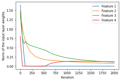
Figure 1: Norm of the connecting weight vectors of input nodes for the IRIS data set with $\lambda=5$ and $\mu=0$.

Table 4: Comparison of Results of the Proposed Feature Selection Method With Those of RCFS, mFSMLP-Cor and SGLC (Results of RCFS, mFSMLP-Cor and SGLC are Directly Collected From )

Datasets	RCFS		mFSMLP-CoR		SGLC			Proposed Method
	Test Acc	Max abs corr	Test Acc	Max abs corr	Test Acc	Average abs corr	Max abs corr	Test Acc	Average abs corr	Max abs corr
Iris	95.4	0.96	94.8	0.42	96.0	0.42	0.96	96.1	0.42	0.42
Thyroid	87.9	0.72	90.7	0.42	94.4	0.41	0.41	94.5	0.43	0.43
WBC	94.6	0.90	95.3	0.69	96.0	0.64	0.69	95.4	0.59	0.59
Sonar	75.4	0.91	77.6	0.63	78.4	0.62	0.79	77.5	0.20	0.62
SRBCT	92.0	0.97	95.0	0.68	95.3	0.59	0.76	95.7	0.21	0.64

Table 5: Group-feature Selection Result

$\bm{\lambda}$	$\bm{\mu}$	Dataset	Test Acc	Distinct # sensors	Average # sensors	Max dep	Avg dep	Dataset	Test Acc	Distinct # sensors	Average # sensors	Max dep	Avg dep
0	0	Iris	96.30	2	2	0.71	0.59	Iris 2	96.00	3	3	0.99	0.75
0	2		95.79	1	1	0	0		95.80	1	1	0	0
0	5		96.00	1	1	0	0		94.77	1	1	0	0
10	0		95.67	1	1	0	0		94.13	1	1	0	0
10	2		95.67	1	1	0	0		94.50	1	1	0	0
10	5		95.30	1	1	0	0		96.19	1	1	0	0
20	0		95.70	1	1	0	0		95.40	1	1	0	0
20	2		96.00	1	1	0	0		94.73	1	1	0	0
20	5		96.67	1	1	0	0		94.26	1	1	0	0
0	0	Smart	92.54	16	16	0.99	0.52	Gas	98.40	16	16	0.99	0.52
0	2	Phone	92.64	7	6.1	0.97	0.46	Sensor	97.61	7	5.5	0.97	0.46
0	5		92.57	6	5.6	0.97	0.46		96.23	5	4.3	0.84	0.43
20	0		91.21	7	5.6	0.97	0.50		97.98	7	6.8	0.97	0.44
20	2		91.27	7	6.8	0.97	0.50		97.68	7	5.5	0.97	0.44
20	5		92.94	7	7	0.97	0.46		94.15	5	3.5	0.68	0.40
50	0		89.40	5	4.5	0.95	0.52		97.76	6	5.8	0.97	0.43
50	2		91.36	7	6.1	0.97	0.50		97.66	6	5.5	0.96	0.44
50	5		91.82	6	6	0.97	0.50		90.84	4	2.7	0.72	0.44
0	0	LRS	82.86	2	2	0.78	0.75	LandSat	84.47	4	4	0.88	0.82
0	2		82.73	2	1.6	0.47	0.45		84.53	4	4	0.88	0.82
0	5		83.75	2	1.4	0.31	0.30		84.60	4	4	0.88	0.82
20	0		83.27	2	1.5	0.39	0.38		84.54	4	4	0.88	0.82
20	2		84.11	2	1.3	0.23	0.22		84.47	4	4	0.88	0.82
20	5		83.60	2	1.2	0.16	0.15		84.54	4	4	0.88	0.82
50	0		83.29	2	1.2	0.16	0.15		84.57	4	4	0.88	0.82
50	2		83.56	2	1.1	0.08	0.07		84.50	4	4	0.88	0.82
50	5		84.06	1	1	0	0		84.54	4	4	0.88	0.82

4.2 Group-feature (sensor) selection results

Table 5 provides a summary of the results on a set of popular data sets for group-feature selection with different values of the parameters $\lambda$, and $\mu$. We now briefly describe the datasets and the groups of features used in this study.

For IRIS data, we group sepal length and width as the first group and the remaining two features as the second group. This is a natural grouping.

The second variant of the Iris dataset, i.e. Iris 2 contains seven features- $f_{1},f_{2},f_{3},f_{4},f_{5}=f_{1}+N(0,0.05),f_{6}=f_{3}+N(0,0.05)$ and $f_{7}=f_{4}+N(0,0.05)$. Thus, for this dataset, the pairs ($f_{1},f_{5}$), ($f_{3},f_{6}$) and ($f_{4},f_{7}$) are strongly correlated. We group these seven features into three groups. The first group contains two features $f_{1}$ and $f_{2}$, the second group consists of three features $f_{5},f_{3}$ and $f_{4}$. The last group has two features $f_{6}$ and $f_{7}$.

The Smartphones dataset is built from recordings of 17 signals of 30 subjects performing six activities (walking, walking upstairs, walking downstairs, sitting, standing, and lying) while wearing a smartphone. Features such as mean, correlation, or autoregressive coefficients were subsequently extracted from these 17 signals. This resulted in 17 feature groups with different number of features in different groups.

The Gas Sensor dataset contains information from 16 chemical sensors exposed to 6 gases at different concentration levels. Each of those 16 sensors provided 8 features, which resulted in a total of 128 features. The goal is to discriminate among the six different gases.

The data set low-resolution spectrometer (LRS) contains 531 high-quality spectra derived from IRAS-LRS database. This data set contains features from two bands, namely blue and red bands. These two bands consist of 44 and 49 flux measurements, respectively. Thus, LRS is a 93-dimensional data set having two groups/sensors.

On the other hand, the LandSat dataset is a variant of the Statlog (Landsat Satellite) dataset, encompassing multi-spectral values of pixels in $3\times 3$ neighborhoods in a satellite image. There are six classes, and the class label corresponds to the center pixel of the $3\times 3$ block. The data set contains images in four spectral bands, each band has nine features corresponding to nine pixel values. We modified this data set by augmenting it with two additional features, the mean and standard deviation of the pixel values of the $3\times 3$ neighborhood, as done in [Chakraborty et al., 2014]. Consequently, the dataset used in our study, referred to as LandSat, consists of four groups, each with 11 features. There are a total of 6435 sample points distributed among the six classes. For our experiments, we utilized 4435 samples for the training set and reserved 2000 samples for testing, following the recommendations from the UCI repository.

Table 5 summarizes the results on these datasets. When only one sensor (group-feature) was selected, we defined the maximum and average dependency of the selected sensor to be zero. This is quite reasonable since if only one sensor is selected, there is NO dependency in the set of selected groups and redundancy is minimized. It is evident that as we increase the value of $\lambda$ or $\mu$, the penalty for redundancy or the group lasso penalty increases. Consequently, a lesser number of groups of features should be selected and also the maximum and average dependency among the selected groups should decrease. Table 5 demonstrates that, except for LandSat, this trend generally holds true across the datasets. But, notably, the impact of the reduced number of features due to higher values of the regularizers on the average accuracy is not much. In fact, with high penalty, in some cases, the test accuracy is also increased. For example, in case of Iris, with the most severe penalty ($\lambda=20,\mu=5$) the test accuracy is marginally better than the case with zero penalty. A similar trend is observed for the LRS dataset.

For LandSat, we have observed from Table 5 that our method is unable to reduce the number of sensors with the threshold $\theta=0.1\times\max_{i}\|\mathbf{v}_{i}\|$. However, from Fig. 2, we can clearly see that the norms of the weights of sensors 1 and 4 are close to each other and are notably higher than those of sensors 2 and 3. From Table 6, we observe that sensors 1 and 4 have the least level of dependency between them, whereas sensors 2 and 3 are highly dependent on all other sensors. These findings (Fig. 2) align with our intended objective. In light of this, instead of using a fixed threshold, it may be more appropriate to select the top two sensors in this particular case. This is what we do when we compare with the existing method(s) - this philosophy also ensures a fair comparison with the results in [Chakraborty et al., 2014] (see Table 7).

Table 6: Group dependency matrix for the LandSat data

Feature-group	1	2	3	4
1	1.00	0.87	0.81	0.69
2	0.88	1.00	0.88	0.79
3	0.79	0.88	1.00	0.88
4	0.68	0.81	0.87	1.00

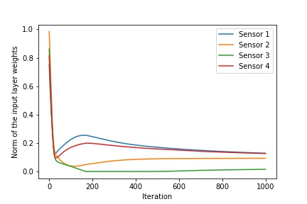
Figure 2: Norm of the connecting weight vectors of input nodes for the LandSat data set with $\lambda=20$ and $\mu=1$.

4.2.1 Comparison with existing method

We now compare our group feature selection results with mGFSMLP-CoR proposed by Chakraborty and Pal [Chakraborty et al., 2014]. To make a fair comparison, the results in Table 7 are attained by using the same number of selected features for both methods. Our implementation follows Algorithm 1, with a slight deviation in line 12. Instead of using a fixed threshold, we select the same number of sensors as the rounded average number of sensors from Table 18 of Chakraborty and Pal [Chakraborty et al., 2014], to obtain the reduced data. We have reported the test accuracy for both methods in Table 7, with the best outcomes highlighted in bold for clarity.

Table 7: Comparison of Results of the Proposed Method With mGFSMLP-CoR (Results of mGFSMLP-CoR are directly collected from [Chakraborty et al., 2014])

Dataset	mGFSMLP-CoR	Proposed Method
Iris	96.07	96.64
Iris 2	96.07	96.58
LRS	88.68	83.86
Gas Sensor	88.80	97.23
LandSat	81.65	84.60

Our method outperforms mGFSMLP-CoR [Chakraborty et al., 2014] in the majority of the datasets (in four out of five datasets). We were unable to implement our method on the other five datasets reported in [Chakraborty et al., 2014], due to the unavailability of those datasets online. Nonetheless, the results obtained on the datasets where our method was applied, suggest its effectiveness in group-feature (sensor) selection with controlled redundancy.

5 Conclusion

In conclusion, this article has introduced an integrated feature selection scheme, that effectively controls the level of redundancy among the selected features, and we have further generalized it for sensor (group-feature) selection. We have also generalized the group lasso regularization and incorporated it alongside the penalty for controlling redundancy for sensor selection, offering a unified method for the selection of feature groups (sensors), which is capable of efficiently eliminating uninformative groups, preserving valuable ones, and keeping control over the level of redundancy. Our proposed regularizers for controlling redundancy in both feature and sensor selection offer an effective and more intuitive approach compared to existing methods. The experimental results on various benchmark datasets demonstrated the effectiveness of the proposed approach. The proposed model achieved competitive performance in terms of classification accuracy while significantly reducing the number of selected features/sensors compared to existing methods. This reduction in feature dimensionality not only improves computational efficiency, but may also enhance interpretability and reduce the risk of overfitting. In this work, the choice of parameters ($\mu\text{ and }\lambda$) has been made in an ad hoc manner, but systematic methods, such as cross-validation can also be used to select these parameters if necessary. Furthermore, the underlying philosophy can be readily extended to other machine learning models, including radial basis function (RBF) networks, offering a versatile tool for feature selection and redundancy control in various applications and domains in the field of machine learning.

References

- [Banerjee and Pal, 2015] Banerjee, M. and Pal, N. R. (2015). Unsupervised feature selection with controlled redundancy (ufescor). IEEE Transactions on Knowledge and data engineering, 27(12):3390–3403.
- [Chakraborty and Pal, 2008] Chakraborty, D. and Pal, N. R. (2008). Selecting useful groups of features in a connectionist framework. IEEE Transactions on Neural Networks, 19(3):381–396.
- [Chakraborty et al., 2014] Chakraborty, R., Lin, C.-T., and Pal, N. R. (2014). Sensor (group feature) selection with controlled redundancy in a connectionist framework. International journal of neural systems, 24(06):1450021.
- [Chakraborty and Pal, 2014] Chakraborty, R. and Pal, N. R. (2014). Feature selection using a neural framework with controlled redundancy. IEEE transactions on neural networks and learning systems, 26(1):35–50.
- [Chen and Zhou, 2010] Chen, X. and Zhou, W. (2010). Smoothing nonlinear conjugate gradient method for image restoration using nonsmooth nonconvex minimization. SIAM Journal on Imaging Sciences, 3(4):765–790.
- [Chung et al., 2017] Chung, I.-F., Chen, Y.-C., and Pal, N. R. (2017). Feature selection with controlled redundancy in a fuzzy rule based framework. IEEE transactions on fuzzy systems, 26(2):734–748.
- [Cong et al., 2016] Cong, Y., Wang, S., Fan, B., Yang, Y., and Yu, H. (2016). Udsfs: Unsupervised deep sparse feature selection. Neurocomputing, 196:150–158.
- [Dash et al., 2002] Dash, M., Choi, K., Scheuermann, P., and Liu, H. (2002). Feature selection for clustering-a filter solution. In 2002 IEEE International Conference on Data Mining, 2002. Proceedings., pages 115–122. IEEE.
- [Du et al., 2016] Du, C., Du, C., Zhe, S., Luo, A., He, Q., and Long, G. (2016). Bayesian group feature selection for support vector learning machines. In Advances in Knowledge Discovery and Data Mining: 20th Pacific-Asia Conference, PAKDD 2016, Auckland, New Zealand, April 19-22, 2016, Proceedings, Part I 20, pages 239–252. Springer.
- [Hall and McMullen, 1992] Hall, D. L. and McMullen, S. A. (1992). Mathematical techniques in multisensor data fusion. artech house. Inc., Norwood, MA, USA, 77.
- [Jenatton et al., 2011] Jenatton, R., Audibert, J.-Y., and Bach, F. (2011). Structured variable selection with sparsity-inducing norms. The Journal of Machine Learning Research, 12:2777–2824.
- [Kang et al., 2021] Kang, Q., Fan, Q., and Zurada, J. M. (2021). Deterministic convergence analysis via smoothing group lasso regularization and adaptive momentum for sigma-pi-sigma neural network. Information Sciences, 553:66–82.
- [Kohavi and John, 1997] Kohavi, R. and John, G. H. (1997). Wrappers for feature subset selection. Artificial intelligence, 97(1-2):273–324.
- [Lazar et al., 2012] Lazar, C., Taminau, J., Meganck, S., Steenhoff, D., Coletta, A., Molter, C., de Schaetzen, V., Duque, R., Bersini, H., and Nowe, A. (2012). A survey on filter techniques for feature selection in gene expression microarray analysis. IEEE/ACM transactions on computational biology and bioinformatics, 9(4):1106–1119.
- [Liu et al., 1996] Liu, H., Setiono, R., et al. (1996). A probabilistic approach to feature selection-a filter solution. In ICML, volume 96, pages 319–327.
- [Meier et al., 2008] Meier, L., Van De Geer, S., and Bühlmann, P. (2008). The group lasso for logistic regression. Journal of the Royal Statistical Society: Series B (Statistical Methodology), 70(1):53–71.
- [Pal and Malpani, 2012] Pal, N. R. and Malpani, M. (2012). Redundancy-constrained feature selection with radial basis function networks. In The 2012 International Joint Conference on Neural Networks (IJCNN), pages 1–8. IEEE.
- [Pang and Xu, 2023] Pang, X. and Xu, Y. (2023). A reconstructed feasible solution-based safe feature elimination rule for expediting multi-task lasso. Information Sciences, 642:119142.
- [Pusponegoro et al., 2017] Pusponegoro, N., Muslim, A., Notodiputro, K., and Sartono, B. (2017). Group lasso for rainfall data modeling in indramayu district, west java, indonesia. Procedia computer science, 116:190–197.
- [Raman et al., 2009] Raman, S., Fuchs, T. J., Wild, P. J., Dahl, E., and Roth, V. (2009). The bayesian group-lasso for analyzing contingency tables. In Proceedings of the 26th Annual International Conference on Machine Learning, pages 881–888.
- [Simon et al., 2013] Simon, N., Friedman, J., Hastie, T., and Tibshirani, R. (2013). A sparse-group lasso. Journal of computational and graphical statistics, 22(2):231–245.
- [Subrahmanya and Shin, 2009] Subrahmanya, N. and Shin, Y. C. (2009). Sparse multiple kernel learning for signal processing applications. IEEE Transactions on Pattern Analysis and Machine Intelligence, 32(5):788–798.
- [Tang et al., 2018] Tang, F., Adam, L., and Si, B. (2018). Group feature selection with multiclass support vector machine. Neurocomputing, 317:42–49.
- [Tibshirani, 1996] Tibshirani, R. (1996). Regression shrinkage and selection via the lasso. Journal of the Royal Statistical Society: Series B (Methodological), 58(1):267–288.
- [Wang et al., 2017a] Wang, J., Cai, Q., Chang, Q., and Zurada, J. M. (2017a). Convergence analyses on sparse feedforward neural networks via group lasso regularization. Information Sciences, 381:250–269.
- [Wang et al., 2017b] Wang, J., Xu, C., Yang, X., and Zurada, J. M. (2017b). A novel pruning algorithm for smoothing feedforward neural networks based on group lasso method. IEEE Transactions on neural networks and learning systems, 29(5):2012–2024.
- [Wang et al., 2020] Wang, J., Zhang, H., Wang, J., Pu, Y., and Pal, N. R. (2020). Feature selection using a neural network with group lasso regularization and controlled redundancy. IEEE transactions on neural networks and learning systems, 32(3):1110–1123.
- [Wang et al., 2022] Wang, Y., Wang, J., and Pal, N. R. (2022). Supervised feature selection via collaborative neurodynamic optimization. IEEE Transactions on Neural Networks and Learning Systems.
- [Yuan and Lin, 2006] Yuan, M. and Lin, Y. (2006). Model selection and estimation in regression with grouped variables. Journal of the Royal Statistical Society: Series B (Statistical Methodology), 68(1):49–67.
- [Yunus et al., 2017] Yunus, M., Asep, S., and Agus, M. S. (2017). Characteristics of group lasso in handling high correlated data. Applied Mathematical Sciences, 11.20:953–961.
- [Zhang et al., 2019] Zhang, H., Wang, J., Sun, Z., Zurada, J. M., and Pal, N. R. (2019). Feature selection for neural networks using group lasso regularization. IEEE Transactions on Knowledge and Data Engineering, 32(4):659–673.
- [Zhang et al., 2017] Zhang, Z., Li, F., Zhao, M., Zhang, L., and Yan, S. (2017). Robust neighborhood preserving projection by nuclear/l2,1-norm regularization for image feature extraction. IEEE Transactions on Image Processing, 26(4):1607–1622.
- [Zhou et al., 2010] Zhou, L., Wang, L., and Shen, C. (2010). Feature selection with redundancy-constrained class separability. IEEE Transactions on Neural Networks, 21(5):853–858.