Co-evolution and Nuclear Structure in the Dwarf Galaxy POX 52 Studied by Multi-wavelength Data From Radio to X-ray

Abstract

The nearby dwarf galaxy POX 52 at $z=0.021$ hosts an active galactic nucleus (AGN) with a black-hole (BH) mass of $M_{\rm BH}\sim 10^{5-6}\,M_{\odot}$ and an Eddington ratio of $\sim$ 0.1–1. This object provides the rare opportunity to study both AGN and host-galaxy properties in a low-mass highly accreting system. To do so, we collected its multi-wavelength data from X-ray to radio. First, we construct a spectral energy distribution, and by fitting it with AGN and host-galaxy components, we constrain AGN-disk and dust-torus components. Then, while considering the AGN-disk emission, we decompose optical HST images. As a result, it is found that a classical bulge component is probably present, and its mass ($M_{\rm bulge}$) is consistent with an expected value from a local relation. Lastly, we analyze new quasi-simultaneous X-ray (0.2–30 keV) data obtained by NuSTAR and XMM-Newton. The X-ray spectrum can be reproduced by multi-color blackbody, warm and hot coronae, and disk and torus reflection components. Based on this, the spin is estimated to be $a_{\rm spin}=0.998_{-0.814}$, which could suggest that most of the current BH mass was achieved by prolonged mass accretion. Given the presence of the bulge, POX 52 would have undergone a galaxy merger, while the $M_{\rm BH}$–$M_{\rm bulge}$ relation and the inferred prolonged accretion could suggest that AGN feedback occurred. Regarding the AGN structure, the spectral slope of the hot corona, its relative strength to the bolometric emission, and the torus structure are found to be consistent with Eddington-ratio dependencies found for nearby AGNs.

1 Introduction

Supermassive black holes (SMBHs) heavier than a million solar masses are believed to be ubiquitously present at the center of the massive galaxies ($>10^{9-10}\,M_{\odot}$, where $M_{\odot}$ is the solar mass) (e.g., Greene, 2012; Miller et al., 2015; Chadayammuri et al., 2023). Various correlations have been found between galaxies and their SMBHs, such as the one between the bulge and SMBH masses (e.g., Magorrian et al., 1998; Gebhardt et al., 2000; Marconi & Hunt, 2003; Gültekin et al., 2009; Kormendy & Ho, 2013), and it has been considered that galaxies and SMBHs have co-evolved. Many studies have been conducted to understand the physical mechanisms responsible for this co-evolution (e.g., Fabian, 2012; King & Pounds, 2015; Harrison et al., 2018, and references therein), especially in massive systems. An often hypothesized scenario is that a galaxy merger ignites star formation (SF) and mass accretion onto an SMBH, and, at some point, the resultant active galactic nucleus (AGN) blows gas out of the system in the form of outflows, preventing further star-formation (SF) and SMBH growth (e.g., Hopkins et al., 2008; Hopkins & Quataert, 2010; Booth & Schaye, 2009). In this scenario, some simulations successfully reproduced the correlations that have actually been observed (e.g., Di Matteo et al., 2005; Croton et al., 2006). In addition to the interplay between the SF and AGN, it has also been proposed that successive mergers are important as they may reduce the scatter around correlations with the SMBH mass (Kormendy & Ho, 2013). However, it is not well understood whether these mechanisms are plausible for less massive systems, or dwarf galaxies with stellar masses of $M_{\rm star}\lesssim 10^{9.5}\,M_{\odot}$.

In considering the growth of dwarf galaxies, many studies have focused on stellar feedback, such as winds, supernovae (SNe), and re-ionization originating in star-forming regions (e.g., Larson, 1974; Efstathiou, 1992; Fitts et al., 2017). The stellar feedback hypothesis has been successful in explaining discrepancies between what the standard lambda cold dark matter ($\Lambda$CDM) model predicts and the actual properties of dwarf galaxies (e.g., substructure, core-cusp, too-big-to-fail, and satellite-plane problems; e.g., Moore et al., 1999; Kroupa et al., 2005; de Blok, 2010; Boylan-Kolchin et al., 2011). On the other hand, AGN feedback has often been ignored, due to various possible reasons, such as the possibility that there is no black hole (BH) that can affect surroundings, the depletion of gas to feed the primary BH due to the stellar feedback, and the difficulty for the BH to sink to the central dense-gas region to grow due to the shallow gravitational potential of the galaxy.

While these assumptions have been used for a long time, recently, an increasing number of works have discussed the importance of AGN feedback theoretically and observationally. By analytically comparing the outflow properties driven by the AGN and SNs, Dashyan et al. (2018) showed that AGN feedback is generally more efficient than the SN feedback (see also Silk, 2017). Cosmological simulations have also shown that the AGN feedback is capable of affecting host galaxy properties (e.g., Koudmani et al., 2021, 2022). Several pieces of observational evidence have supported this idea. An increasing number of AGNs have been found in dwarf galaxies (e.g., Greene & Ho, 2004, 2007; Greene et al., 2020, and references therein). Penny et al. (2018) found ionized gas that does not follow the dynamical structure of the stellar component and suggested that it is perhaps due to the AGN Manzano-King et al. (2019); Mezcua & Domínguez Sánchez (2020). Also, Liu et al. (2020) detected ionized gas outflows from about 90% of AGN-hosting dwarf galaxies, and suggested that the outflows are likely due to the AGNs. Finally, it was found that dwarf galaxies together with massive systems form a $M_{\rm BH}$–$M_{\rm bulge}$ relation, which could suggest the co-evolution even in the less massive systems (e.g., Schutte et al., 2019; Greene et al., 2020).

Studying AGNs in dwarf galaxies is important not only in the above context, but also for revealing the properties of intermediate-mass BH (IMBH) AGNs (i.e., $M_{\rm BH}\sim 10^{3-6}\,M_{\odot}$; e.g., Mezcua, 2017). In fact, it is still unclear whether IMBH AGNs have similar nuclear structures (e.g., the corona, accretion disk, and torus) to those of massive AGNs and whether they follow the same observational trends as suggested for the massive AGNs. Ultimately, the understanding of IMBH AGNs is expected to play an important role in linking the accretion physics between stellar-mass BH and SMBHs. Furthermore, in terms of application, if constrained, its spectral energy distribution (SED) will serve as a useful template for discussing the strategy to detect IMBH AGNs at different redshifts, including the seeds of quasars at high redshifts of $\gtrsim$ 6 (Cruz et al., 2023). The search for the quasar progenitors with various observatories is being actively discussed (e.g., Valiante et al., 2018; Marchesi et al., 2020; Griffin et al., 2020).

In this paper, toward a better understanding of the co-evolution and AGN structures in less massive systems, we present our observational study of the dwarf galaxy POX 52 located at (R.A., Decl.) = (12h02m56.913s, $-$20d56m02.66s) in J2000.0 (e.g., Kunth et al. 1981). POX 52 is in the nearby Universe of $z=$ 0.021, or $D=93$ Mpc, adopting a $\Lambda$CDM cosmology with $H_{0}$ = 70 km s^-1 Mpc^-1, $\Omega_{\rm m}=0.3$, and $\Omega_{\Lambda}=0.7$, and is known to host a rapidly growing type-1 IMBH AGN with a BH mass of $M_{\rm BH}\approx 2$–$4\times 10^{5}\,M_{\odot}$ and an Eddington ratio of $\lambda_{\rm Edd}\approx$ 0.2–0.5 (Thornton et al., 2008). The mass was derived by the single-epoch method, and the bolometric luminosity necessary for the Eddington ratio was derived by integrating an SED roughly fitted to observed data from the radio to the X-ray. The galaxy, thus, provides us with an invaluable opportunity to reveal both AGN and host-galaxy properties precisely. This single-object study is complementary to studies using large samples, given that we reveal the nature of the IMBH AGN in quite detail.

We collected multi-wavelength data, including newly obtained broadband X-ray data by NuSTAR and XMM-Newton quasi-simultaneous observations. Our analysis based on these data can be divided into three parts essentially and proceeded as follows. First, we constructed an SED from infrared (IR) to ultra-violet (UV) and decomposed it into AGN and host-galaxy components using the Code Investigating GALaxy Emission (CIGALE) code (Boquien et al., 2019) (Section 3). The AGN components were the radiation from the accretion disk and that from the dust torus. Next, we spatially resolved high-resolution Hubble Space Telescope (HST) images into AGN and host-galaxy components (Section 4). Here, in order to avoid the degeneracy of the AGN and host-galaxy components, the AGN component was included so that it was consistent with the SED result. Finally, we analyzed a broadband X-ray spectrum obtained with NuSTAR and XMM-Newton (Section 6). Our fits to the spectrum took into account the reflection component expected from the dust torus constrained by the SED decomposition, enabling us to reduce degeneracy with other spectral components. In summary, starting from the SED results, we reveal the properties of the host galaxy and the AGN while ensuring no inconsistencies in all the used data.

This paper is organized as follows. We present the data used and how these were reduced and/or reprocessed in Section 2. Next, as described previously, Sections 3, 4, and 6 present our SED, imaging, and X-ray data analyses, respectively. We revisit the IMBH mass estimate in Section 5. Using our new results, we discuss the evolution of POX 52 and the AGN structure, and summarize our AGN SED model in Section 7. Our summary of this paper is finally presented in Section 8. Unless otherwise noted, errors are quoted at the 1$\sigma$ confidence level for a single parameter of interest.

2 Observational Data

2.1 Data used for constructing an SED

2.1.1 XMM-Newton Optical and UV Data

Using XMM-Newton (Jansen et al., 2001), we obtained X-ray, optical, and UV data (ID = 0890430101) with an exposure of $\approx$ 20 ks between 2021 December 30 and 31. The data were analyzed with the Science Analysis Software (SAS) version 20.0.0 by following the XMM-Newton ABC guide. The latest calibration files were used. The Optical Monitor (OM) onboard XMM-Newton obtained data in the Image+Fast mode from optical to UV using all the available filters ($V$, $B$, $U$, UVW1, UVM2, and UVW2). The obtained data in the Image and Fast modes were reprocessed with omichain and omfchain, respectively. By inspecting the data in the Image mode, it was found that the background levels around POX 52 were enhanced in the images in the $V$, $B$, $U$, and UVW1 filters because of stray light caused by the reflection of a star outside the field of view and bad pixels in the source regions. Thus, we decided not to use the photometric data in these four bands. For the two remaining bands (UVM2 and UVW2), we measured source count rates with the SAS task omphotom; we fitted a PSF to the image while considering the background level inferred from an annulus between five and ten pixels. The count rates were then converted into flux densities based on the factors suggested by the XMM-Newton User Guide. The obtained flux densities were then corrected for dust extinction by adopting the extinction law of Cardelli et al. (1989) with $R_{\rm V}$ = 3.1 and $E(B$–$V)$ = 0.05. The resultant flux densities in the UVM2 and UVW2 bands are $0.21\pm 0.01$ mJy and $0.25\pm 0.02$ mJy, respectively. We mention that this extinction correction was applied to the other photometric data from UV to near-IR wavelengths as well. Regarding the Fast-mode data, a lightcurve was created in each filter and was examined to assess whether the emission varied significantly during each $\approx$ 3 ks exposure by fitting a constant model using the chi-square method. We found that no significant variations were present, given the $p$-values $>0.1$ recovered.

2.1.2 GALEX Data

We used the GALEX GR6/7 Data Release:10.17909/T9H59D (catalog 10.17909/T9H59D) to cover the FUV (1516 Å) and NUV (2267 Å) bands (Martin et al., 2005; Bianchi et al., 2017), which was used also by Thornton et al. (2008). The magnitudes derived by adopting an aperture with a radius of 4″ were adopted. The respective magnitudes are 19.10$\pm$0.14 mag and 18.79$\pm$0.07 mag in the AB system. Hereafter, all magnitudes are presented in the same system. By considering the aperture correction ($\Delta m=-0.10$ for the FUV band, and $\Delta m=-0.12$ for the NUV band) and dust extinction, the resultant flux densities were calculated to be 0.13$\pm$0.02 mJy and 0.20$\pm$0.02 mJy in the FUV and NUV bands, respectively.

2.1.3 PanSTARRS Data

We utilized PanSTARRS data to add optical flux densities to our SED (Chambers et al., 2016; Flewelling et al., 2020). We adopted the Mean-object catalog, released in the PS1 DR2:10.17909/s0zg-jx37 (catalog 10.17909/s0zg-jx37). In the catalog, POX 52 was identified as an extended source. Thus, to estimate the flux of the entire galaxy, we adopted magnitudes derived in the Kron photometry and corrected them by considering that the Kron magnitude within 2.5 $\times$ 1st radial moment generally underestimates the entire flux by $\sim$ 10%. The $g$-, $r$-, $i$-, $z$-, and $y$-Kron magnitudes listed in the catalog are 17.29 mag, 16.89 mag, 16.76 mag, 16.65 mag, and 16.52 mag, and the flux densities corrected for the aperture and dust extinction were estimated to be 0.578$\pm$0.002 mJy, 0.800$\pm$0.004 mJy, 0.876$\pm$0.008 mJy, 0.948$\pm$0.010 mJy, and 1.06$\pm$0.01 mJy, respectively.

2.1.4 2MASS Data

To cover the near-IR band, we used the photometry data of the Two Micron All Sky Survey (2MASS) All-Sky Point Source Catalog (Skrutskie et al., 2006) in the same manner as Thornton et al. (2008). We note that POX 52 was not listed in the Extended Source Catalog. The observed magnitudes in the $J$, $H$, and $Ks$ bands (i.e., 1.24 $\mu$m, 1.66 $\mu$m, and 2.16 $\mu$m) are 15.72$\pm$0.08 mag, 14.96$\pm$0.08 mag, and 14.46$\pm$0.08 mag. These magnitudes were derived by a profile-fitting method, and the normalizations were adjusted to include the entire fluxes. By correcting the observed values for dust extinction, the flux densities in the $J$, $H$, and $Ks$ bands were estimated to be 0.86$\pm$0.06 mJy, 1.09$\pm$0.08 mJy, and 1.12$\pm$0.09 mJy, respectively.

2.1.5 WISE Data

In the IR band, we used WISE photometric data in the four bands: 3.4 $\mu$m, 4.6 $\mu$m, 12 $\mu$m, and 22 $\mu$m ($W1$, $W2$, $W3$, and $W4$, respectively). POX 52 was detected in all bands in the ALLWISE Source Catalog (Wright et al., 2010; Mainzer et al., 2011), and its WISE data were used in a low-mass AGN study by Marleau et al. (2017). As no bad flags were raised, we used the listed photometric data: 13.82$\pm$0.03 mag, 13.23$\pm$0.03 mag, 10.07$\pm$0.06 mag, and 7.49$\pm$0.13 mag in the $W1$, $W2$, $W3$, and $W4$ bands, respectively. These were derived with a profile-fitting method, appropriate for a point source and POX 52 as well, because POX 52 is identified as a point source in the catalog (ext_flg = 0). We then converted them into flux densities by assuming coefficients appropriate for a power-law function of $S_{\nu}\propto\nu^{-2}$ ($S_{\nu}$ represents flux density). The flux densities were found to be $0.92\pm 0.02$ mJy, $0.87\pm 0.02$ mJy, $2.90\pm 0.16$ mJy, and $8.5\pm 1.0$ mJy, in the $W1$, $W2$, $W3$, and $W4$ bands, respectively.

2.1.6 Spitzer Data

To put stronger constraints on the emission in the IR band, we also used Spitzer/IRS spectral data provided by the CASSIS catalog (Lebouteiller et al., 2011, 2015). The spectrum was investigated by Hood et al. (2017), and many emission lines were identified by them. Among the lines, [Ne V] at $\lambda=$ 14.32 $\mu$m and 24.32 $\mu$m and [O IV] at $\lambda=$ 25.89 $\mu$m would be associated with AGN radiation given photons with energies $\gtrsim 50$ eV are necessary to produce them. In our SED analysis, we used the CIGALE code (Boquien et al., 2019, Section 3), and this code does not take into account AGN-related emission lines. Thus, we excluded the wavelength bands around the [Ne V] and [O IV] lines. Specifically, the 14.4–14.9 $\mu$m and 23.6–27.8 $\mu$m ranges were excluded. Also, to reduce the computational cost, we rebinned the spectrum so that each bin size was 0.2 $\mu$m.

We mention here two points: the high-ionization potential lines seen in the IRS spectrum are unlikely to contribute much to the WISE W3 and W4 fluxes, and the Spitzer/IRS spectrum would accommodate the entire galaxy. For the first point, we calculated the equivalent widths (EWs) of [Ne V] 14.32 $\mu$m, [Ne V] 24.32 $\mu$m, and [O IV] 25.89 $\mu$m lines to be $\sim$ 0.2 $\mu$m, $\sim$ 0.2 $\mu$m, and $\sim$ 1 $\mu$m. Here, we used the line fluxes measured by Spoon et al. (2022). It is thus clear that the [Ne V] 14.32 $\mu$m line contributes little to the flux in the W3 band, whose effective bandwidth is $\approx$ 5.5 $\mu$m. On the other hand, in the W4 band with the effective bandwidth of $\approx$ 4.1 $\mu$m, the [O IV] 25.89 $\mu$m line, in particular, is relatively large (i.e., $\sim$ 30%). However, given that the response is significantly low around the [O IV] line, its contribution to the flux can be safely ignored. For the second point, Figure 3 shows the W3 and W4 flux densities as well as the IRS spectrum. It is clearly seen that the two WISE fluxes and the adjacent IRS fluxes are comparable. As the WISE fluxes were measured for the entire galaxy, we concluded that no aperture correction was needed for the IRS spectrum.

2.1.7 VLA Data

Very Large Array (VLA) data in the $S$ and $C$ bands are available. The $S$-band ($\approx$ 3 GHz) data were taken in the course of the VLA sky survey (VLASS; Gordon et al., 2020, 2021). The survey data were already analyzed by a VLASS team, and reconstructed images are available in the VLASS website. By examining an image encompassing POX 52, we found no significant emission from the source position. Thus, using noise in an off-source region, the upper limit at a $3\sigma$ level was estimated to be 0.6 mJy beam^-1, where beam size is $\sim$ 2$\farcs$5. The corresponding upper-limit luminosity is $\lesssim 2\times 10^{37}$ erg s^-1.

The $C$-band ($\approx$ 5 GHz) data were obtained by a pointing observation, and were analyzed by Thornton et al. (2008), who found that no significant emission was detected by the $C$-band observation. The 3$\sigma$ upper limit was estimated to be 0.08 mJy, or $4\times 10^{36}$ erg s^-1, by the authors, and we used this limit.

2.2 HST Data

We used HST data with the goal of revealing stellar components of the host galaxy by fitting the images. POX 52 was observed with the Advanced Camera for Surveys (ACS) and the High Resolution Channel (HRC) on 2004 November 19 and 18. Two optical filters of F435W and F814W were adopted in the respective days, and the data were analyzed by Thornton et al. (2008) in the past. We used the data stored in the archive of Mikulski Archive for Space Telescopes (the data are available at MAST:10.17909/J2EW-NH46 (catalog 10.17909/J2EW-NH46)). The entire exposure in each filter was split into five intervals, each having calibrated and flat-fielded images. We combined the five calibrated images into one with an HST pipeline of astrodrizzle, where final_scale was set to 0$\farcs$025. We again run astrodrizzle to produce a noise image relevant to each image by setting final_wht_type to ERR (e.g., Floyd et al., 2008; Kokubo & Minezaki, 2020). The noise images were necessary to perform the GALFIT fitting (Peng et al., 2002, 2010) in Section 4. The total exposures of the combined data in the F435W and F814W filters are $\approx$ 2.6 ks and $\approx$ 2.5 ks, respectively. In addition to producing the observed images and the relevant noise images, we generated a PSF image in each filter using a PSF modeling software of TinyTim (Krist et al., 2011). These images were also necessary for the image fit.

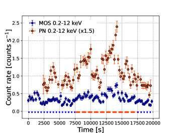
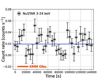
Figure 1: Left: XMM-Newton MOS (blue) and PN (orange) lightcurves in the 0.2–12 keV band. The adopted binsize is 200 sec. For clarity, the PN lightcurve is increased by a factor of 1.5. The blue dotted and orange dashed lines indicate fainter and brighter phases, we defined in Section 6.4. Right: NuSTAR lightcurve in the 3–24 keV band, created with a binsize of 4 ks. The blue solid line corresponds to the average value, and the orange solid line indicates when the XMM-Newton observation was executed.

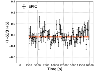
Figure 2: XMM-Newton/EPIC hardness ratios, defined as (H-S)/(H+S), where S and H are count rates in the 0.2–1 keV and 1–12 keV bands. The adopted binsize is 200 sec. The orange line indicates the constant model fitted to the data.

2.3 X-ray Spectra and Light-curves

2.3.1 XMM-Newton X-ray Data

The raw XMM-Newton MOS and PN data in the X-ray band were initially reprocessed using emproc and epproc, respectively. To filter periods with high background counts, we created lightcurves of the MOS1 and MOS2 above 10 keV with PATTERN=0 (single events) and a PN one in the 10–12 keV band with the same pattern selection. For the MOS1 and MOS2 data, we adopted the threshold of 0.30 counts s^-1 to define their good time intervals (GTIs). For the PN data, by inspecting the PN lightcurve, we left only the period when the count rates were less than 0.45 counts s^-1 as the GTI. Because the PN data were affected by a strong background flare and the tail of the flare could not be removed completely with the simple filter described above, we also excluded the events around the flare. Finally, by applying a PATTERN selection of $\leq$ 4 plus FLAG=0 and $\leq$ 12 to the PN and MOS data, respectively, we obtained cleaned data. Source events were then extracted from circular regions of radii 30″and 40″, respectively. Similarly, background count rates were estimated from off-source regions with radii of 30″and 120″, respectively. The background-subtracted MOS and PN lightcurves are shown in Figure 1. Based on the count rate in each detector, we confirmed that pile-up effects are negligible. The hardness ratios shown in Figure 2 were calculated in each bin by combining the MOS and PN data (i.e., periods when good PN data were unavailable were not considered). No significant variability of the hardness ratios was confirmed by fitting a constant model and obtaining a $p$-value of $>0.01$. Spectra were extracted from the same source and background regions. The MOS1 and MOS2 spectra were combined into one using epicspeccombine. We then binned the source spectra to have a minimum of one count per bin. Response files were produced using the SAS tasks arfgen and rmfgen. Particularly in generating the arf files, a flag was raised for applyabsfluxcorr to correct the effective area to remove residuals between NuSTAR and XMM-Newton spectra.

2.4 NuSTAR Data

NuSTAR (Harrison et al., 2013) observed the target for $\approx$ 80 ks quasi-simultaneously with XMM-Newton (ID = 60701047002). The NuSTAR observation started around 5 ks later than the XMM-Newton one. Following the “NuSTAR Analysis Quickstart Guide”, we used the standard nupipeline script in the NuSTARDAS version v2.1.2 for the reprocessing. We set SAAMODE=optimized, since the background event rates were slightly elevated around the South Atlantic Anomaly. We used the reduced data for further analyses. We note that although we created different reduced data with more strict options of SAAMODE=strict and TENTACLE=yes, we found that the resultant spectra and lightcurves were similar to those obtained for SAAMODE=optimized.

We defined the source region as a 40″-radius circle centered at the optical position, by taking account of the FWHM of the NuSTAR PSF ($\approx$18″). For the background region, we adopted an off-source circular region with a 120″-radius on the same detector. Then, we produced lightcurves, spectra, and response files using the nuproducts task. The produced lightcurves in the 3–24 keV range are shown in the right panel of Figure 1. Significant variability was found by fitting a constant model to the data and obtaining a $p$-value of 3$\times 10^{-4}$. It was, however, confirmed that the flux level during the XMM-Newton observation was consistent with that for the entire NuSTAR observation within $\sim$ 1$\sigma$. Thus, Thus, our NuSTAR spectra, to be fitted with the XMM-Newton spectrum, were produced by combining all data in each detector (i.e., FPMA and FPMB). Each of the two spectra was then binned using the same approach we adopted for the XMM-Newton spectra.

Table 1: Allowed Parameter Grids in the SED Fitting and Best-fit Parameters

Parameter	Grids	Best
delayed SFH
$\tau_{\rm main}$ [Myr]	1,000, 3,000, 6,000	3000
age [Myr]	2500, 5000, 7500, 10000	7500
SSP (Bruzual & Charlot, 2003)
IMF	Chabrier (2003)	…
Metallicity	0.004, 0.008, 0.02	0.004
Nebular emission (Inoue, 2011)
$\log\,U$	$-2.0$	…
Metallicity	0.004 (fixed to the SSP one)	…
Dust attenuation (Charlot & Fall, 2000)
$A_{\rm V,ISM}$	0.2, 0.4, 0.6, 0.8	0.6
AGN emission (Stalevski et al., 2016)
$\tau_{\rm 9.7}$	3, 5, 9	3
$p_{\rm torus}$	1.0	…
$q_{\rm torus}$	1.0	…
$\sigma_{\rm torus}$ [$\arcdeg$]	20, 10	10
$R_{\rm torus}$	20	…
$\theta_{\rm inc}$ [$\arcdeg$]	20, 30, 40	20
$f_{\rm AGN}$	0.005, 0.01, 0.5	0.01
disk type	Schartmann et al. (2005)	…
Dust emission (Draine et al., 2014)
$q_{\rm pah}$	0.47, 1.12, 2.50	1.12
$u_{\rm min}$	5, 25, 50	25
$\alpha$	2	…
Other Best-fit Parameters
SFR	…	0.15$\pm 0.01\,M_{\odot}$ yr-1
$M^{\rm old}_{\rm star}$	…	$8.3\pm 0.4\times 10^{8}\,M_{\odot}$
$M^{\rm young}_{\rm star}$	…	$1.4\pm 0.1\times 10^{6}\,M_{\odot}$

Note. — For a detailed explanation, we guide readers to the CIGALE papers of Boquien et al. (2019) and Yang et al. (2020). The second and third columns indicate the parameter grids used to fit the SED and the obtained best-fit parameters, respectively.

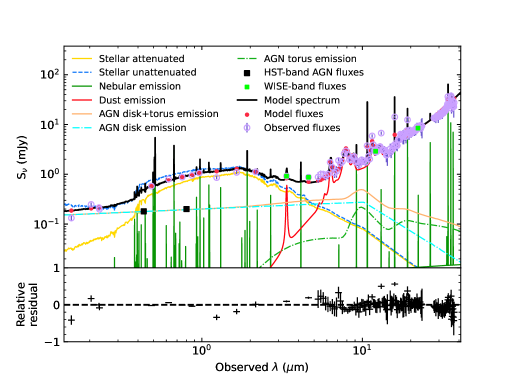
Figure 3: SED of POX 52 (purple open circles), fitted by a model (black line), which includes stellar emission, nebular emission, dust emission originating in the SF, and AGN disk and torus emission. Corresponding lines are denoted in the figure. The black-filled squares indicate the fluxes adopted to model the AGN emission in resolving the HST images into AGN and host-galaxy components (see Section 4). Also, the WISE-band fluxes are shown with green squares so that one can distinguish between the WISE and Spitzer/IRS data. The lower panel indicates residuals, defined as the difference between the observed and model fluxes divided by the observed one.

3 SED analysis

With the CIGALE code (Boquien et al., 2019), we decomposed our constructed SED (Figure 3) consisting of the collected flux densities from the IR to the UV. We did not consider the radio and X-ray data in our SED analysis. The radio data are later used to discuss whether the upper limits are consistent with the results of our SED analysis, while the X-rays were not considered since they require complex models to take into account all their futures. A detailed analysis of the broad-band X-ray spectrum is reported in Section 6.

CIGALE can compute SED models from IR to UV in a self-consistent framework, keeping the energy between the UV/optical and IR wavelengths balanced. Among emitting mechanisms and objects whose modes are implemented in CIGALE, we considered SF, stars, AGN disk emission, and AGN dusty torus emission, as listed in Table 1. The SF history was assumed to decrease exponentially with an e-folding time (i.e., sfhdelayed; e.g., Ciesla et al., 2015, 2016). To reproduce emission due to SF, we selected the single-stellar-population model of bc03 (Bruzual & Charlot, 2003), and the IMF of Chabrier (2003). The standard nebular emission model (nebular) associated with the stellar model was also incorporated. To model dust attenuation of the host-galaxy emission, we adopted the model constructed by following the procedure proposed in Charlot & Fall (2000) (dustatt_modified_CF00). Radiation from old stars (age $>10$ Myr) is attenuated by dust in the interstellar medium (ISM), while that from younger stars is additionally subject to dust attenuation in a birth cloud (BC). The two dust-attenuation models in the ISM and the BCs are represented by power-laws normalized to the amount of attenuation in the $V$-band, which was left as the free parameter. The power-law indices for the ISM and BC sites were set to the canonical values of $-0.7$ and $-1.3$. The amounts of $V$-band attenuation for the young and old stars were linked as $A^{\rm ISM}_{\rm V}/(A^{\rm ISM}_{\rm V}+A^{\rm BC}_{\rm V})=0.44$. The dust emission from the host galaxy was modeled with dl2014 created by following Draine et al. (2014), which is the refined model of Draine & Li (2007). The parameters were set while considering recent works (Buat et al., 2018, 2021). The dust fraction in photo-dissociation regions was fixed to 0.02 (e.g., Draine & Li, 2007). Next, we modeled the AGN torus and disk emission using SKIRTOR (i.e., skirtor2016; Stalevski et al., 2016), assuming a two-phase medium torus model where high-density clumps distribute in a low-density region. The parameters are the torus optical depth at 9.7 $\mu$m ($\tau_{9.7}$), the torus density radial parameter ($p_{\rm torus}$), the torus density angular parameter ($q_{\rm torus}$), the angle between the equatorial plane and the edge of the torus ($\sigma_{\rm torus}$), the ratio of the maximum to minimum radii of the torus ($R_{\rm torus}$), the inclination angle ($\theta_{\rm inc}$), and the AGN fraction of the total IR luminosity ($f_{\rm AGN}$). Using the parameter settings and grids listed in Table 1, we fitted the above-described models. The best-fit parameters are also listed in the table. For a sanity check, we performed the CIGLAE mock analysis; this analysis initially simulates photometric data based on the best-fit components and the observed photometric uncertainties, and then fits the adopted components to assess whether the best-fit parameters can be recovered even for the simulated data (e.g., Yang et al., 2020). We then confirmed that the best-fit parameters can be surely recovered.

We confirm that the best-fit model is consistent with the properties in the radio and X-ray bands. The SFR of POX 52 is estimated to be $\approx$ 0.15 $M_{\odot}$ yr^-1 at $z\approx 0.02$, and corresponds to $4\times 10^{36}$ erg s^-1 at 1.4 GHz via a relation in Kennicutt & Evans (2012). For an index of 0.8 typical for star-forming galaxies (Tabatabaei et al., 2017), the corresponding luminosities at 3 GHz and 5 GHz were $\approx$ 4–5$\times 10^{36}$ erg s^-1. These are consistent with the upper limits constrained in the $S$- and $C$-band VLA observations. Regarding the AGN, its radio luminosity should be below $4\times 10^{36}$ erg s^-1 as well. As the 2–10 keV luminosity of the AGN is $\sim 10^{42}$ erg s^-1 (Section 6), the X-ray radio loudness defined as $L_{\rm 1.4}/L_{\rm 2-10}$ should be $<4\times 10^{-6}$. This is consistent with observed radio loudnesses of radio-quiet AGNs (Panessa et al., 2015). In summary, our SED fit does not contradict the radio upper limits and, also, the limits suggest that the AGN is radio quiet.

The parameters constrained by the SED analysis, particularly, the AGN parameters, played very important roles in decomposing the HST images and also in the X-ray spectral analysis. Details are described in Sections 4 and 6.

4 HST Image Decomposition

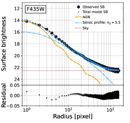
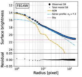
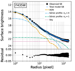
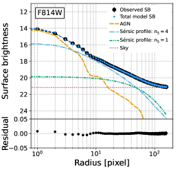
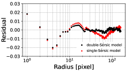
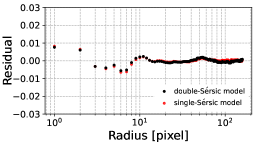
Figure 4: Top panels: Surface brightness radial profiles obtained from the HST observation with the F435W and F814W filters. Each profile is reproduced by a model consisting of the AGN (i.e., PSF), Sérsic-profile, and sky components. These were fitted by using the GALFIT code. One pixel corresponds to 0$\farcs$025 ($\approx$ 11 pc). Each lower window shows residuals, or (model – data)/data values. Middle panels: Same as the top panels, but for the double-Sérsic model, where a Sérsic profile is added to the model used in the upper panels. Bottom panels: Comparisons of the residuals obtained by the single- and double-Sérsic profiles in the two filters. For clarity, uncertainties are not shown.

Table 2: Best-fit Parameters of the Fits to the HST images

	Parameter	F435W	F814W	Units
Point Source (AGN)
(1)	$m$	$18.44^{\dagger}$	$18.22^{\dagger}$	mag
Single Sérsic Profile
(2)	$m$	18.17	16.19	mag
(3)	$n_{\rm S}$	5.5	7.3	…
(4)	$R_{\rm e}$	16.3	120	pix
(5)	$b/a$	0.88	0.88	…
(6)	$PA$	1.5	37.4	°
First Sérsic Profile
(7)	$m$	18.53	17.37	mag
(8)	$n_{\rm S}$	4†	4†	…
(9)	$R_{\rm e}$	8.8	19.7	pix
(10)	$b/a$	0.84	0.97	…
(11)	$PA$	$-$2.3	3.5	°
Second Sérsic Profile
(12)	$m$	18.96	17.97	mag
(13)	$n_{\rm S}$	1†	1†	…
(14)	$R_{\rm e}$	93.4	72.1	pix
(15)	$b/a$	0.79	0.68	…
(16)	$PA$	55.3	41.7	°
(17)	$B/T$	0.60	0.63	…

Note. — (1) Total magnitude of the point-source model. (2,3,4,5,6) Total magnitude, Sérsic index, half-light radius (1 pix = 0″025 $\approx$ 11 pc), axis ratio, and position angle of a Sérsic model fitted to the data together with the point-source and sky background components (i.e., single-Sérsic model). (7)–(16) Sérsic-function parameters for the double-Sérsic model. (17) Bulge-to-total flux ratio for the double-Sérsic model. ^†These parameters were fixed in the GALFIT fits.

We decomposed each of the HST images taken with the two filters (F435W and F814W) into AGN and host-galaxy components using the image fitting code of GALFIT (Peng et al., 2002, 2010). First, as a simple model, we considered a point-source component and a Sérsic function to represent AGN and stellar emission, respectively. Adding a sky background component furthermore, we fitted the HST images while leaving all possible parameters as free parameters. The result was that the total magnitudes of the point source were largely different between the two adjacent bands (i.e., $\Delta m\approx 1.5$). To avoid this probably unreasonable result, in each band, we fixed the AGN contribution by referring to the AGN disk flux density constrained by the SED analysis. The actual magnitudes we adopted were 18.44 mag and 18.22 mag in the F435 and F814W filters, respectively. Also, the AGN position was fixed to the peak in each image. Under these conditions, the HST images in the F435W and F814 filters seemed to be reproduced well with the Sérsic indices ($n_{\rm S}$) of 5.5 and 7.3, respectively, as shown in the top panels of Figure 4. The best-fit parameters of the fitted single-Sérsic models are listed in Table 2. Although the indices are slightly higher than the past estimates of $\sim 4$ based on ground-based images by Barth et al. (2004) and those by Thornton et al. (2008) using the same HST images, all estimated values ($n_{\rm S}\gtrsim 4$) could suggest that the stellar emission is dominated by a bulge (e.g., Meert et al., 2015).

We furthermore added a Sérsic function to the above model to assess whether there was an additional component, such as a disk component, occasionally presumed to have $n_{\rm S}\sim 1$ (e.g., Allen et al., 2006; Mendel et al., 2014). If none or only one of the Sérsic indices is fixed, an unreasonable result is obtained; for example, in the case of fixing only the index of one Sérsic component to $n_{\rm S}=1$, the other Sérsic index was constrained to be $n_{\rm S}\sim$ 2 for the F435W data, and a much larger value of $n_{\rm S}\sim$ 6 was obtained for the F814W data. Therefore, we fixed one of the two Sérsic indices to 1 and the other to 4. The results of fitting this double-Sérsic model to the surface brightness profiles are shown in the middle panels of Figure 4, and the best-fit parameters are listed in Table 2. To compare the goodness-of-fits of the double-Sérsic and single-Sérsic models, in the lower panels of Figure 4, we plot the residuals, or (model – data)/data, left by the two models for each filter. As seen for the F435W data more clearly, the double-Sérsic model seems to fit the data better than the single-Sérsic one. This is suggested by a decreased chi-square value by an order of 1000 for the addition of six free parameters. A similar improvement was found for the F814 data. A caveat here is that these face values should be taken with caution, given that additional systematic uncertainty would be present in both data and model and mitigate the difference in the chi-square value. We lastly comment that the half-light radii constrained by the single-Sérsic model in the two bands differ by almost one order of magnitude, while such a difference is not seen for the double-Sérsic model. This perhaps suggests that the double-Sérsic model is preferable. However, to draw a robust conclusion on whether there are really two distinct Sérsic components or not, for example, spatially resolved spectroscopy will be helpful, as it might be able to disentangle the components kinematically.

In this paper, we preferentially adopt the results obtained by the double-Sérsic model for discussions by considering its better description of the data and the similarity of the constrained parameters between the two bands. We, however, do not exclude the single-Sérsic model. To show more on the good fits of the double-Sérsic model, Figure 5 displays observed images, models, and their differences normalized by data counts. In addition, a result to be remarked on the double-Sérsic model is that the Sérsic profile with $n_{\rm S}=4$ may represent the “classical” bulge; the bulge-to-total flux ratios ($B/T$) in both bands are $\approx 0.6$ under the assumption that the profile with $n_{\rm S}=4$ is a bulge component, and the values fall in an expected range for the classical bulge (Gao et al., 2022).

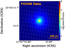
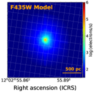
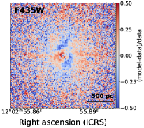
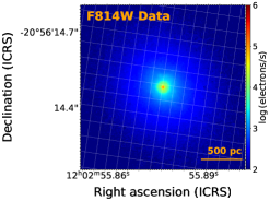
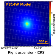
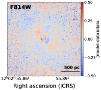
Figure 5: Upper panels: From left to right, observed image, fitted model, and residual (difference divided by data counts) image in the F435W band. Lower panels: Same as the upper panels, but for the F814W band.

The overall radial profiles seem to be well reproduced by the double-Sérsic model as well as the single-Sérsic one, as shown so far, but residuals, or (model – data)/data, of $\sim 0.02$ are present at inner several pixels in both models (Figure 4). To quantitatively examine whether the residuals may be explained by systematic uncertainty in the PSF modeling, we analyzed HST/HRC F435W and F814W data of GD 153, which is a white dwarf and can be assumed to be a point source. The data we analyzed were taken in 2004 February 15 and 2005 May 19, within which the HST data of POX 52 were obtained. In the same procedures as adopted for POX 52, we reprocessed the HST data and fitted the images with a PSF model and a sky-background model. We then found that, in both data, residuals of $\approx$ 0.03 remain, particularly in the inner pixels ($\lesssim$ 10 pix). Such residuals may be due to systematic uncertainties in the PSFs, and would explain the residuals found for POX 52.

Last but not least, we investigated what fitting results can be obtained for different assumptions on the fixed AGN magnitudes. Indeed, the AGN flux estimated by the SED fit is likely to be different from that during the HST observations, due to intrinsic time variation. Possible variability can be inferred from the structure function (a measure of the ensemble rms magnitude difference as a function of the time difference between observations). Baldassare et al. (2020) calculated the values of low-mass AGNs to be $0.2$ at most. Thus, we fitted each HST image by changing the magnitude of the AGN component by $\pm$0.2 mag. As a result, for the single-Sérsic model, the Sérsic index was estimated to be $\gtrsim 4$ in both images. Also, in the case of the double-Sérsic model, the $B/T$ ratios were estimated to be within 0.5–0.6, consistent with the above-derived values of $\approx$ 0.6. In summary, the impact is confirmed to be minor for our discussions.

5 Estimate of the BH mass

We describe here our estimate of the BH mass of POX 52, since it is important for explaining our modeling of the X-ray spectra. We estimated the BH mass based on the so-called single-epoch method (e.g., Vestergaard, 2002; Vestergaard & Peterson, 2006; Greene & Ho, 2005), for which an AGN luminosity and the width of a broad emission line are necessary. For the luminosity, we used the AGN luminosity at 5100Å  of $\lambda L_{\lambda,\rm 5100}$= 1.1$\times 10^{42}$ erg s^-1, which was constrained from the SED analysis and was confirmed to fit the surface brightnesses reasonably (Sections 3 and 4). The uncertainty derived by CIGALE, as well as that inferred from the HST analysis, is $\sim$ a few percentages. The broad emission line we adopted was H$\beta$, and, from Barth et al. (2004), we took the full width at half maximum of $v_{\rm FWHM}=$ 760$\pm$30 km s^-1. We substituted the two values to a calibrated equation used in the previous study of Thornton et al. (2008), which referred to Bentz et al. 2006 and Onken et al. 2004:

$$M_{\rm BH}=1.05\times 10^{7}(\lambda L_{\lambda,5100}/10^{44}{\rm erg\,s}^{-1})^{0.518}$$ (1)

$$\times(v_{\rm FWHM}/10^{3}{\rm km\,s}^{-1})^{2}M_{\odot}.$$

The mass was then estimated to be $\log(M_{\rm BH}/M_{\odot})\approx 5.8$. As its error, we consider 0.5 dex or a factor of three, which is a canonical one and is dominated by systematic uncertainty (e.g., Vestergaard & Peterson, 2006; Ricci et al., 2022). Uncertainty should be present due to the measurements of the AGN luminosity and the line width in the different epochs. However, this would be negligible compared to 0.5 dex, given a possibly small structure function of $<0.2$ for low-mass AGNs (Baldassare et al., 2020). Our estimated mass is slightly higher than the past one of $\log(M_{\rm BH}/M_{\odot})\approx 5.5$–5.6 by Thornton et al. (2008). This is because the AGN luminosity we used is 2–3 times higher than the past one of Thornton et al. (2008), whose estimate was also based on a fit to the same F435W data. We rely on our estimate because, as described above, our AGN-luminosity measurement would be more reliable given that it fits the SED and also HST images. An additional reason is because the newly estimated mass is more favorable for interpreting X-ray results, as described in the next section. Finally, we mention that Thornton et al. (2008) concluded that they could underestimate the luminosity. They found that the $B-I$ color of the galaxy components (i.e., two Sérsic profiles) that they fitted to the HST data was bluer than those of galaxies appropriate for comparison (e.g., Im galaxies) and interpreted the bluer color being due to the contamination of the AGN emission to the Sérsic components. Here, as lessons learned, we suggest that the SED analysis plays an important role in disentangling the AGN and host-galaxy components in the image fit. For further discussion, we adopt our mass estimate (i.e., $\log(M_{\rm BH}/M_{\odot})\approx 5.8\pm 0.5$) as our fiducial value.

6 X-ray Spectral and Timing Analysis

To facilitate understanding of our X-ray analysis, we describe its flow here. We first jointly fitted the spectra obtained by the quasi-simultaneous NuSTAR and XMM-Newton observations (Section 6.1). The spectra were averaged over the exposure times. The observation period of XMM-Newton covers only part of the longer NuSTAR observation (the right panel of Figure 1), but the flux measured by NuSTAR for the partial period and the one for the whole period are similar. Thus, the spectral variation between the periods with and without XMM-Newton could be neglected. The energy bands for XMM-Newton and NuSTAR we considered were 0.2–12 keV and 3–30 keV, respectively. Events above 30 keV were dominated by the background emission, and the spectra in that range were not considered. Since the spectral analysis alone was not sufficient to determine the final spectral model, we also discuss the X-ray variability during the course of our spectral analysis (Section 6.2). Finally, we proceeded to the determination of the most plausible model (Section 6.3). After this analysis, we also discuss whether the time variability of the spectrum and the archival spectra can be readily explained by the model (Section 6.4 and 6.5).

6.1 Simple Model Fitting

As a baseline model, we considered the absorption by our galaxy and the primary X-ray power-law component with a high-energy cutoff originating in a hot corona around the IMBH; i.e., tbabs*zhighect*zpowerlw in the XSPEC terminology. The galactic absorption was fixed to $N_{\rm H}^{\mathrm{Gal}}\,=3.9\times 10^{20}$ cm^-2, derived using the HEADAS nh task (Kalberla et al., 2005). The photon index and normalization of the power-law component were left as free parameters, while the cutoff was fixed at 200 keV, typical for nearby AGNs (e.g., Ricci et al., 2018). By adopting the $C$-statistic method (Cash, 1979), we fitted the model and found that the baseline model left clear excesses in the soft ($<$ 1 keV) and hard ($>$ 10 keV) bands, as shown in the top-left panel of Figure 6. Here, the resultant $C$ value is 2914.8 for the degrees of freedom (d.o.f.) of 2782.

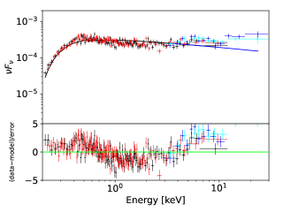
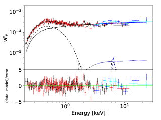
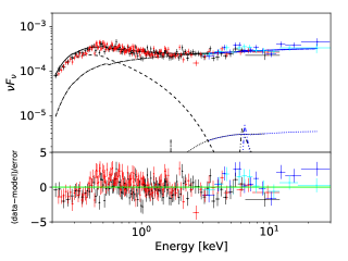
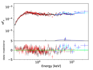
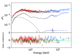
Figure 6: Top-left: XMM-Newton (black and red crosses) and NuSTAR (blue and cyan crosses) spectra fitted by an absorbed power-law model ($C$/d.o.f. = 2914.8/2782). Residuals are shown below the spectra. Top-right: Improved fit by adding disk-blackbody (diskbb) and torus components ($C$/d.o.f. = 2510.4/2780), appearing particularly in the soft ($<$ 2 keV) and hard band ($>2$ keV), respectively. Middle-left: Fitting result by replacing the disk-blackbody component with the warm corona model (thcomp*diskbb; $C$/d.o.f. = 2578.3/2778). Middle-right: Spectra fitted by replacing the warm corona model with a disk-reflection component (relxilllpCp; $C$/d.o.f. = 2532.0/2779). The primary power-law emission and reflected emission are shown as a combined component. Bottom: Fitted by our final model consisting of the warm corona, power-law, disk-reflection, and torus-reflection components ($C$/d.o.f. = 2489.0/2775).

To better reproduce the soft-band spectral feature, we added diskbb (Mitsuda et al., 1984), often used to phenomenologically reproduce similar soft excesses of Seyfert galaxies (e.g., Middei et al., 2020; Jiang et al., 2020; Xu et al., 2021). The model computes the spectrum from a standard accretion disk for a given temperature at the innermost radius. For the hard band excess, we incorporated torus emission. The torus absorbs and scatters X-rays, producing a hump around 30 keV, and a fraction of the absorbed X-rays result in fluorescent emission lines (e.g., the Fe line at 6.4 keV). The torus emission was, indeed, suggested by the result of the SED analysis. It is natural to consider the same torus geometry used in the SED analysis; it is the SKIRTOR torus model, which considers a two-layer structure (Stalevski et al., 2016), but there was no X-ray model that was built by considering the geometry. Therefore, we decided to alternatively adopt the clumpy torus structure, whose models were available in both IR and X-ray band (Miyaji et al., 2019; Yamada et al., 2023). We adopted the IR one of Nenkova et al. (2008a) (see also Nenkova et al., 2008b) and the X-ray one of Tanimoto et al. (2019). First, we investigated with what parameters the IR clumpy torus of Nenkova et al. (2008a) can reproduce a spectrum close to that of our best-fit SKIRTOR model by varying clumpy-torus parameters: the ratio of inner and outer radii ($R_{\rm clump}$), the optical depth for each cloud ($\tau_{\rm V,\rm clump}$), the number of clouds along the equatorial plane ($N_{\rm clump}$), the radial-density-profile index ($q_{\rm clump}$), the angular width ($\sigma_{\rm clump}$), and the inclination angle ($\theta_{\rm inc}$). As a result, we found that the SKIRTOR-like spectrum was able to be reproduced with $R_{\rm clump}=$ 20, $\tau_{\rm V,\rm clump}=$ 40, $N_{\rm clump}=1$, $q_{\rm clump}=$ 0.5, $\sigma_{\rm clump}=$ 15°, and $\theta_{\rm inc}=$ 20°. A comparison between the SKIRTOR and clumpy torus models was also discussed by Yamada et al. (2023), and a similar conclusion was drawn by the authors. We note that we relied on the SKIRTOR model in the SED fitting, as it has been generally used in CIGALE and makes it easy to compare our result with other ones. The IR-torus geometrical parameters were then used to define our X-ray torus model, having hydrogen column density along the equatorial plane ($N^{\rm eqn}_{\rm H}$), torus angular width ($\sigma_{\rm clump}$), and inclination angle ($\theta_{\rm inc}$) as parameters. The column density was derived by converting the visual extinction of each clump to a column density under the assumption of a Galactic $N_{\rm H}$-to-$A_{\rm V}$ ratio (Draine, 2003) and by substituting the column density and also the number of clumps to Equation 5 of Tanimoto et al. (2019). The equatorial column density was estimated to be $N^{\rm eqn}_{\rm H}\sim 10^{23}$ cm^-2. The two other parameters were simply fixed to the equivalent values of the IR torus model (i.e., $\theta_{\rm inc}$ and $\sigma_{\rm clump}$). As we set the incident X-ray spectrum to the primary X-ray one, no free parameters were left for the X-ray torus model. By adding these soft-excess and torus models, we obtained a much better fit with the $C=$ 2510.4 (i.e., $\Delta C\approx-400$) for the additional two free parameters (d.o.f. = 2780). The best-fit result shown in the top-right panel of Figure 6 indicates that the soft excess is well reproduced by the diskbb model. On the other hand, the power-law emission becomes dominant in the X-ray band above $\approx$ 3 keV rather than the torus emission, while the weak torus emission is consistent with no clear narrow Fe-K$\alpha$ emission at 6.4 keV.

Although we obtained the good fit, we suggest that a different model is necessary, in particular, to describe the soft excess. The temperature of the diskbb component was constrained to be $\sim 160$ eV. This is much higher than theoretically expected one of $\sim$ 20–30 eV for the standard disk model (e.g., Shakura & Sunyaev, 1973; Kubota et al., 1998; Mallick et al., 2022) where the inner edge extends down to the inner stable circular orbit (ISCO) for the spin parameter ($a_{\rm spin}$) of 0, $M_{\rm BH}\approx 6\times 10^{5}\,M_{\odot}$, and the bolometric luminosity of $\sim 10^{43}$ erg s^-1. Thus, the diskbb component does not represent the inner part of the standard accretion disk, as established for basically all AGNs. This is also indicated from the normalization of the diskbb component; the normalization was constrained to be $\approx$ 65, and the corresponding inner radius of the disk was estimated to be $\approx 8\times 10^{9}$ cm following Kubota et al. (1998), much smaller than expected from the ISCO of $\approx 5\times 10^{11}$ cm. We note that if we adopted bbody instead of diskbb, a temperature of $\approx$ 110 eV was obtained. Interestingly, this is consistent with a typical value measured for hard-X-ray selected type-1 AGNs, in spite of distinct difference in $M_{\rm BH}$ (Ricci et al., 2017a).

6.2 Insight into Soft-excess Emission from the Flux Variation

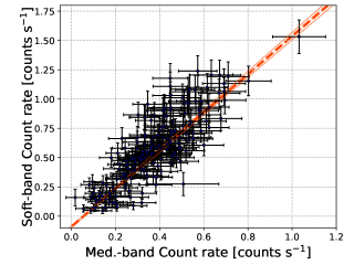
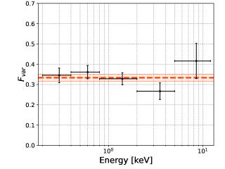
Figure 7: Top: Relation between the count rates in two bands of 0.2–1 keV and 1–12 keV, denoted as Soft-band and Med.-band, respectively. Each count rate is derived with a binsize of 100 sec, and all three detectors (MOS1, MOS2, and PN) are taken into consideration. The linear regression line is drawn in orange together with the area corresponding to the 1$\sigma$ error. Bottom: Fractional variability spectrum created with lightcurves with a binsize of 200 sec. This spectrum is consistent with being a constant model, as described by the orange dashed lines together with the 1$\sigma$ error.

To better understand what alternative component can be used for the soft excess, we focused on flux variation. Studying the variation, previous works have estimated the spatial scale of the soft-excess emitting region (e.g., Noda et al., 2013a; Kammoun et al., 2015; Lewin et al., 2022), and we adopted the simple but powerful method of Noda et al. (2011). Their method is first to examine linear correlations of the count rate in a highly variable band (e.g., $\sim$ 1–3 keV; Noda et al., 2013b, 2014) with those in different bands and then to reveal a component that follows the highly variable emission and the other stable component. Applying this method to five nearby ($z\lesssim 0.1$) Seyfert galaxies, Noda et al. (2013a) found a soft-excess component that did not vary synchronously with the primary power-law emission on a time scale of several hundred ks and concluded that it originated in a radius larger than several hundred gravitational radii.

Following Noda et al. (2011), we examined the correlation between 0.2–1 keV and 1–12 keV count rates for POX 52, as shown in Figure 7. The binsize was set to 100 sec so that almost all bins had at least a few counts. The result indicates that an offset for the soft-band count rate, which would have suggested the presence of a stable component, was not found. The same conclusion can be drawn even if we adopt similar energy bands (e.g., 0.2–1 keV vs. 1–3 keV) to those used by Noda et al. (2011). Thus, the soft excess could have varied on a time scale of 100 sec, or perhaps less, while following the power-law component. A consistent result was obtained by making a fractional variability spectrum with a similar binsize of 200 sec (Vaughan et al., 2003). This larger binsize was necessary, to keep photon counts in each of the divided energy channels. The spectrum in Figure 7 was well reproduced with a constant model, consistent with the idea that fluxes across energy bands vary in a similar fashion within the time scale. These results suggest that the soft-excess emission originates in a region close to the IMBH, specifically, $r\lesssim 17\,R_{\rm g}$, or $\lesssim 3\,R_{\rm ISCO}$ if $a_{\rm spin}=0$ and $\lesssim 13\,R_{\rm ISCO}$ if $a_{\rm spin}=0.998$.

6.3 Final Model

Based on the above time-variability analyses, we tested two models. One was a warm corona model, and the other was an ionized-disk-reflection model. These have been often discussed as the origin of soft excesses seen in type-1 AGNs (e.g., Petrucci et al., 2013; Boissay et al., 2016; Petrucci et al., 2018; Kubota & Done, 2018). In the warm corona scenario, such a secondary coronal component is usually presumed to cover a fraction of the accretion disk and, if the disk extends down closely to the central IMBH and the corona covers the inner region, rapid variability may be expected. Also, such a corona is optically thicker and cooler (i.e., $\tau_{\rm warm}\sim 10$ and $kT_{\rm e,warm}\sim 1$ keV) than the hot corona responsible for the primary X-ray emission, and the spectrum of the warm corona model is generally harder than the disk thermal emission. Thus, it has the potential to reproduce the hot spectral feature revealed by fitting the diskbb model with $kT\sim 160$ eV previously. On the other hand, the reflection model produces emission lines in the inner part of the ionized disk, and the blurring of the lines due to the relativistic effects results in the soft-excess-like spectrum (e.g., Ross & Fabian, 2005; Crummy et al., 2006). This is also expected to vary rapidly, given that it originates in the vicinity of the BH.

We mention that, as a model to reproduce the soft-excess emission, a partial covering model is sometimes adopted, and we tested whether zxipcf can improve our final model presented in Section 6.3.3. We then confirmed that the partial covering model did not improve the fit significantly (i.e., $\Delta C\approx-4$ for $\Delta$ d.o.f. = 3).

6.3.1 Warm Corona Model

We examined the validity of the warm corona model. The warm-corona Comptonization was modeled by thcomp with multi-temperature blackbody emission from the accretion disk as the seed-photon spectrum. The seed spectrum was modeled with diskpbb, which is different from diskbb, since it allows the user to vary the temperature distribution. In fact, the disk thermal emission has already been constrained in the SED analysis up to the UV region (Section 3), and some parameters of diskpbb were fixed so that it is consistent with our SED model. Specifically, by comparing the SED model and the diskbpbb spectrum in the optical/UV band ($\approx$ 0.1–1 $\mu$m), the normalization was fixed to 1.73$\times 10^{6}$ and the power-law index that determines the temperature distribution was fixed to 0.637 (i.e., $p_{\rm disk}$ in $T\propto r^{-p_{\rm disk}}$). As a result, the free parameters of thcomp*diskpbb were the temperature at the inner edge of the disk, the optical thickness and temperature of the Comptonizing corona, and the covering factor of the corona.

The result of our fit is shown in the middle-left panel of Figure 6. The temperature of the inner edge of the disk was constrained to be $\sim$ 30 eV, being in good agreement with the theoretically expected one for the disk reaching the ISCO. The $C$ value ($C$/d.o.f. = 2578.3/2778) is, however, worse than that obtained by adopting only the diskbb model. Also, the inconsistency between the model and the data is evident in the figure, particularly below 0.4 keV. These facts would suggest that an alternative model is necessary to reproduce the data correctly.

6.3.2 Disk Reflection Model

We examined an ionized-disk-reflection model by using the relxilllpCp model (Dauser et al., 2014; García et al., 2014). This model calculates reflected emission while considering relativistic effects. This was replaced with the power-law component, as the model returns both the primary power-law component and its reflected emission on the disk by executing a self-consistent calculation. Among the parameters to be set in the disk model, the inclination angle, the disk density, and the electron temperature of the corona, were fixed at 20°, $10^{15}$ cm^-3, and 100 keV, respectively. The free parameters were the spin value, the inner radius, the photon index of the incident power-law spectrum, the ionization parameter, and the normalization. The other parameters were set to their default values. The resulting fit is shown in the middle-right panel of Figure 6. With fewer free parameters, this disk-reflection model better described the spectra ($C$/d.o.f. = 2532.0/2779) than the warm-corona model. However, the model appears to overestimate the data around 2–3 keV and slightly underestimate the data in other bands. Also, this disk-reflection model would be incomplete, because it should be natural to expect the contribution of the tail of the thermal disk emission if the disk extends to the vicinity of the central IMBH and that of possibly associated Comptonization emission, like type-1 AGNs. Therefore, we further tested the model considering both Comptonization and disk-reflected emission, as detailed in the next subsection.

6.3.3 Combined Model

As a physically reasonable model for our broad-band X-ray data, we combined disk thermal emission, Comptonization, and disk-reflection and torus emission; i.e., thcomp*diskpbb + relxilllpCp + [torus emission]. While some of the parameters were fixed, similarly to what was done in the previous sections, we changed the disk density from $10^{15}$ cm^-3 to $10^{15.5}$ cm^-3. The main reason is clarified in the next paragraph. The best-fit model is shown in the bottom panel of Figure 6, where the power-law and reflected components are plotted separately for clarity. Reduced residuals are readily seen in the figure, and, in fact, the fit was significantly improved ($C$/d.o.f. = 2489.0/2775), compared with the disk-reflection model. The best-fit parameters obtained with this spectral model are summarized in Table 3. Here, to mitigate the degeneracy between the disk reflection relxilllpCp and the other disk emission (thcomp*diskpbb), we fixed the parameters of the latter emission and allowed only its normalization to vary synchronously with the disk emission in calculating errors. This is motivated by the result that the 0.2–1 keV and 1–12 keV emission varied in a similar fashion. The result suggests that the IMBH could spin rapidly ($a_{\rm spin}\approx 0.998_{-0.814}$, where the error corresponds to a 90% confidence interval) and the inner radius of the reflecting disk is $3.2\,R_{\rm ISCO}$ (i.e., $\approx 4.0\,R_{\rm g}\sim 4\times 10^{11}$ cm).

We suggest that the composite model is reasonable as, in addition to the better statistical value, no clear discrepancy exists between the constrained parameters. The thermal disk model (diskpbb) indicates the inner radius of the thermal disk to be $\sim 10^{12}$ cm ($\approx 7.2\,R_{\rm g}$) and the temperature at the disk inner-edge to be $\approx 24$ eV. These values are consistent with those inferred by the disk-reflection model (relxilllpCp); the inner radius of the disk is $\sim 10^{11}$–$10^{12}$ cm (the uncertainty in $M_{\rm BH}$ is taken into consideration), and the temperature expected at the radius is $\sim 30$ eV. In addition, the ionization parameter indicated by the disk-reflection model is $\log\xi\approx 2.8$, and a consistent value can be derived by considering the disk density ($n_{\rm e}=10^{15.5}$ cm^-3), irradiating X-ray luminosity ($\approx 10^{42}$ erg s^-1), and the inner radius of the disk ($\sim 10^{11}$–$10^{12}$ cm). Here, we note two things. If a smaller BH mass (i.e., $M_{\rm BH}\approx 2$–4$\times 10^{5}\,M_{\odot}$; Thornton et al., 2008) is adopted, the inner-edge of the reflecting disk becomes smaller than inferred by the thermal disk emission, suggesting that the thermal disk cannot serve as the reflector. Thus, the larger mass is preferable. Also, if the disk density (i.e., $10^{15.5}$ cm^-3) is not changed from the default value of $10^{15}$ cm^-3, the calculated ionization can be higher than that suggested by the disk-reflection model. Thus, an increased density is favored. In summary, the model describes the broadband spectra without any difficulty in the parameters, and we treat it as our final model.

Table 3: Best-fit Parameters Obtained by Final Model

	Parameter	Best-fit	Units
Galactic absorption
(1)	$N^{\rm Gal}_{\rm H}$	$3.9\times 10^{-2\,\dagger}$	1022 cm-2
Comptonization of Multi-BB. emission (thcomp*diskpbb)
(2)	$\tau_{\rm warm}$	21‡	…
(3)	$kT_{\rm e,warm}$	0.34‡	keV
(4)	$f_{\rm c,warm}$	0.10‡	…
(5)	$kT_{\rm e,disk}$	0.024‡	keV
(6)	$p_{\rm disk}$	0.637†	…
Disk reflection (relxilllpCp)
(7)	$\theta_{\rm inc}$	20†	degrees
(8)	$a_{\rm spin}$	$0.998_{-0.814}$	…
(9)	$r_{\rm in}$	3.2${}^{+1.5}_{-2.2}$	ISCO
(10)	$\Gamma$	$1.98^{+0.04}_{-0.05}$	…
(11)	$\log\xi_{\rm ion}$	$2.8\pm 0.3$	…
(12)	$n_{\rm disk}$	$10^{15.5\,\dagger}$	cm-3
(13)	$kT^{\rm PL}_{\rm e}$	$100^{\dagger}$	keV
(14)	Norm	$6.0^{+0.6}_{-0.5}\times 10^{-6}$	…
Torus reflection
(15)	$N^{\rm Eqn}_{\rm H}$	$10^{23\,\dagger}$	cm-2
(16)	$\sigma_{\rm clump}$	$15^{\dagger}$	degrees
(17)	$\theta_{\rm inc}$	$20^{\dagger}$	degrees
Flux and Luminosity
(18)	$F_{\rm 0.5-2}$	6.3	10-13 erg cm-2 s-1
(19)	$F_{\rm 2-10}$	6.7	10-13 erg cm-2 s-1
(20)	$F_{\rm 10-30}$	6.4	10-13 erg cm-2 s-1
(21)	$L^{\rm Comp}_{\rm 0.5-2}$	5.9	1040 erg s-1
(22)	$L^{\rm PL}_{\rm 2-10}$	4.9	1041 erg s-1
Statistical parameters
(23)	$C$/d.o.f.	2489.0/2775	…

Note. — (1) Absorbing hydrogen column density due to our Galaxy in the sightline. (2,3,4) Optical depth, electron temperature, and covering factor of the warm corona. (5,6) Temperature at the inner edge of the disk and temperature-distribution index of the thermal disk component, providing seed photons to the warm corona. (7) Inclination angle from the polar axis of the disk. (8) Spin parameter. (9) Inner radius of the disk. (10) Photon index of the primary power-law emission. (11) Ionization parameter. (12) Disk density. (13) Temperature of electrons responsible for the power-law emission. (14) Normalization. (15,16,17) Hydrogen column density along the equatorial plane, torus angular width, and inclination angle of the torus model. (18,19,20) Observed 0.5–2 keV, 2–10 keV, and 10–30 keV fluxes. (21) Luminosity of the warm corona emission in the 0.5–2 keV band. (22) Luminosity of the power-law, or hot corona, emission in the 2–10 keV band. (23) $C$-statistic value versus d.o.f. Here, errors are quoted at the 90% confidence level, following a convention in the X-ray analysis. ^†These parameters were fixed. ^‡ These parameters were fixed in calculating the other errors. See Section 6.3.3 for more details.

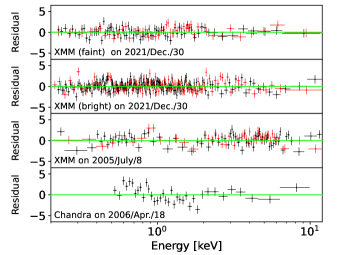
Figure 8: The first and second panels show residuals obtained when we fitted the final model to the XMM-Newton spectra in the fainter and brighter phases. The third one shows residuals obtained by fitting the final model to the past XMM-Newton spectra. The last one shows residuals between the past Chandra spectrum and our final fitted model.

6.4 Spectral Variability

The XMM-Newton lightcurve shows strong variability (Figure 1), and thus, it is important to investigate whether the variation was the result of a change in the normalization or whether some other spectral parameters changed. To identify the reason, the observation period was divided into brighter and fainter phases, as indicated by blue and orange lines in Figure 1, and spectral fitting was performed in each phase. We eventually found that only by allowing the normalization of the entire model, except for the torus emission, to change freely, the spectra in the bright and faint periods can be fitted well without any clear residuals (Figure 8), or with $C$/d.o.f. = 1474.5/1767 and $C$/d.o.f. = 991.2/1186, respectively.

6.5 Archival X-ray Spectra

We finally assessed whether the final model could reproduce X-ray spectra obtained by previous X-ray observations carried out with XMM-Newton on 2005 July 8 and Chandra on 2006 April 18. The observation IDs of the XMM-Newton and Chandra data are 0302420101 and 5736, respectively. These data were analyzed by Thornton et al. (2008), and following their procedure, we extracted the source spectra from the XMM-Newton/EPIC data in the 0.2–12 keV band and that from the Chandra/ACIS data in the 0.5–7 keV band. To show that our model is plausible, we fitted the spectra with fewer free parameters. Specifically, for the Chandra spectrum, we allowed only the entire normalization of the model to change freely. The fits resulted in $C$/d.o.f. = 421.2/356. While the statistical value is not as good as in the previous fits, clear residuals are not seen (Figure 8). Regarding the XMM-Newton spectra, we included a partially covering ionized gas absorber model (zxipcf), whose presence in the spectra was already suggested by Thornton et al. (2008). In the same way, as adopted for the Chandra spectrum, only the overall normalization and parameters relevant to the zxcipcf model were allowed to vary freely. We obtained a good fit ($C$/d.o.f. = 1466.429/1801; see also Figure 8). Between the spectra, including our new one, the X-ray flux varied; the 2–10 keV flux observed by Chandra was slightly higher by a factor of $\approx$ 1.1 than that during our new observations. In contrast, the flux during the past XMM-Newton observation was $\approx$ 2.5 times lower. Even if corrected for the partial absorption, the flux was still 1.6 times lower. Thus, it was found that, in spite of the flux variation by a factor of $\sim 2$, our final model can reasonably fit the past spectra as well.

7 Discussion

We have comprehensively revealed both host-galaxy and AGN properties based on the SED fit (Section 3), the optical image fits (Section 4), and the X-ray spectral and timing analyses (Section 6). With the constraints obtained, we initially discuss the evolution of the system in Section 7.1. Then, we discuss the AGN structure in detail in Section 7.2. Finally, we summarize our overall AGN SED from the IR to the X-ray in Section 7.3.

7.1 Galaxy and Central IMBH Evolution

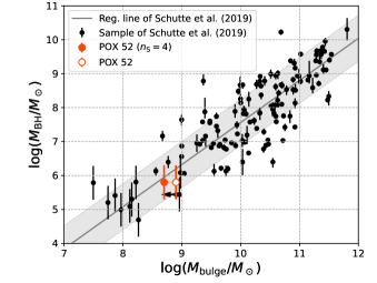
Figure 9: BH mass versus bulge mass. Two orange dots are plotted for POX 52. The filled one corresponds to the bulge mass that considers only the Sérsic component with $n_{\rm S}=4$ in the double-Sérsic model (Section 4), while the unfilled one is the stellar mass derived by the SED analysis without any consideration of the imaging analysis. Galaxies investigated by Schutte et al. (2019) are shown as black dots. Although POX 52 was included in their galaxy sample, the corresponding data point is removed here. The line and shaded area indicate a regression line and one standard deviation (0.68 dex), derived by Schutte et al. (2019) for their sample.

Our SED analysis suggests that the SF activity peaked possibly around $\sim$ 7.5 Gyrs ago, corresponding to $z\sim$ 1. As expected from this inference, the old stellar population ($>$ 10 Myr) with a mass of $M^{\rm old}_{\rm star}\approx 8.3\times 10^{8}$ $M_{\odot}$ dominates the entire stellar mass (i.e., $M_{\rm star}\approx M^{\rm old}_{\rm star}$), while the mass of young stars is $M^{\rm young}_{\rm star}\sim 10^{6}\,M_{\odot}$. Related to this, the HST imaging analysis has given us an important insight into the host galaxy by finding that the classical bulge is the important structure. It is thus suggested that the bulge could have started to form at $z\sim 1$, and POX 52 could have experienced a galaxy merger(s), given that the classical bulge is expected to be the result of the merger (e.g., Naab & Burkert, 2003; Hopkins et al., 2010). Currently at $z\approx 0.02$, the host galaxy of POX 52 can be categorized as a star-forming galaxy given the SFR of 0.15 $M_{\odot}$ yr^-1 ($-$0.8 in a log scale) and the main sequence derived by Whitaker et al. (2012). The main sequence at $z<0.5$ predicts an SFR for galaxies around the stellar mass of POX 52 to be $10^{-0.4}$ $M_{\odot}$ yr^-1 with a scatter of 0.34 dex, and this is consistent with the estimated SFR within $\approx$ 1$\sigma$.

The BH spin could provide important information on the growth history of the central BH, as suggested by numerical simulations (e.g., Volonteri et al., 2005; Berti & Volonteri, 2008). The BH spin can reach its maximum value of $\approx$ 0.998, if the mass becomes about three times its initial value via prolonged accretion (Thorne, 1974). In contrast, if multiple BH mergers or stochastic accretion flows are the dominant way of growing for the BH, a lower spin value is expected on average. Although there is a very large uncertainty, the spin value was constrained to be $a_{\rm spin}=0.998_{-0.814}$, which could suggest that the last growth episode was due to prolonged gas accretion. If this is true, the IMBH should have released the energy efficiently, perhaps affecting the host galaxy (i.e., through AGN feedback). Given the possible relation between the SF and AGN activity, AGN feedback could have been important around the peak of the SF ($z\sim$ 1). Here, we suspect that the current AGN activity would not be tightly linked to the presumed activity around $z\sim 1$, because an accretion episode since then at rates above the current one ($\lambda_{\rm Edd}\sim$ 0.3) would result in a mass of $\gg 1\times 10^{6}\,M_{\odot}$ (Salpeter, 1964). This is much larger than the current mass. Thus, it is likely that the current level of activity has been intermittent or has started recently. To reveal the actual mechanism that is feeding the central IMBH, it would be useful to study the properties of the cold molecular gas, which is the likely source of the AGN feeding (e.g., Yamada, 1994; Monje et al., 2011; Izumi et al., 2016; Shangguan et al., 2020; Kawamuro et al., 2021).

To further investigate whether the host galaxy and the central IMBH of POX 52 have co-evolved while affecting each other, it is important to analyze the location of POX 52 in the bulge/BH mass plot. We estimate the bulge mass to be $5.2$–$5.5\times 10^{8}\,M_{\odot}$ by adopting the total stellar mass of $8.7\times 10^{8}\,M_{\odot}$ and the bulge-to-total flux ratio of $B/T=$ 0.60–0.63 derivable from the analysis of the HST data (Table 2). Our bulge mass is smaller than the previous ones of $\sim$1–2$\times 10^{9}\,M_{\odot}$ (Barth et al., 2004; Thornton et al., 2008; Schutte et al., 2019), and also our fiducial IMBH mass is $\log(M_{\rm BH}/M_{\odot})\approx 5.8$, heavier than those estimated in the previous studies (Barth et al., 2004; Thornton et al., 2008). As shown in Figure 9, our results show that POX 52 follows the $M_{\rm BH}$–$M_{\rm bulge}$ relation that was constrained by Schutte et al. (2019) down to $M_{\rm BH}\sim 10^{5}\,M_{\odot}$ and $M_{\rm bulge}\sim 10^{8}\,M_{\odot}$. This conclusion remains, even if no stellar decomposition is considered, or we adopt the single-Sérsic model result. This is indicated in Figure 9 as well. In addition, we find that with our estimates, POX 52 almost perfectly follows the relation between $M_{\rm BH}$ and $M_{\rm star}$ determined for early-type galaxies down to $M_{\rm star}\sim 10^{9}\,M_{\odot}$ by Greene et al. (2020).

The fact that POX 52 follows the $M_{\rm BH}$–$M_{\rm bulge}$ and $M_{\rm BH}$–$M_{\rm star}$ relations could suggest that the central IMBH and host galaxy may have influenced each other. Koudmani et al. (2021) investigated the $M_{\rm BH}$–$M_{\rm star}$ scaling relation using FABLE, simulating the cosmological growth of galaxies and BHs, with a particular focus on dwarf galaxies, and found that simulated BH masses tend to be smaller than expected by the observed relation. The authors suggested that the reason may be that the stellar feedback is too strong, which inhibits the growth of BHs (see also Trebitsch et al., 2018; Bellovary et al., 2019; Koudmani et al., 2019). The prescription of the stellar feedback was based on that of Vogelsberger et al. (2013), which succeeded in explaining the observed properties of the galaxies (e.g., cosmic SFR history and stellar mass function). Later, Koudmani et al. (2022) reported results for different assumptions on the stellar feedback. Among their various simulation setups, they showed that BHs would have larger masses than expected from the observed $M_{\rm BH}$–$M_{\rm star}$ relation, especially in conditions where BH accretion can get close to the Eddington limit ($\lambda_{\rm Edd}\gtrsim 0.1$). This is due to the rapid growth of the BH and the suppression of SF by the AGN feedback. In addition, the authors also showed that less mass accretion rate onto a BH ($\lambda_{\rm Edd}\lesssim 0.01$) may be compatible with the $M_{\rm BH}$–$M_{\rm star}$ relation (see Figures 2 and 8 of Koudmani et al., 2022). Although the stellar mass range studied by Koudmani et al. (2022) ($M_{\rm star}\sim 10^{5}$–$10^{8}\,M_{\odot}$) was smaller than the mass of POX 52 ($M_{\rm star}\sim 10^{9}\,M_{\odot}$) by one order of magnitude, so we should be careful about relying on the results, POX 52 and the observed relation could be reproduced if there was no extreme stellar feedback and moderate BH accretion, or AGN feedback, took place (see also Sharma et al., 2022).

In summary, POX 52 would have experienced a galaxy merger(s), forming the classical bulge, and the IMBH has reached the current mass possibly through gas accretion at some point. Given that POX 52 follows a $M_{\rm BH}$–$M_{\rm bulge}$ relation and the IMBH could have released accreting energy efficiently, AGN feedback could have taken place. The current level of AGN activity is, however, likely short-lived, and unrelated to the main channel of growth of the system. The feeding mechanism at work now is unclear and, to reveal it, more data, especially cold molecular gas data, are necessary.

7.2 AGN Structure

X-ray data are important for revealing the structures of the AGN, especially in the vicinity of the central BH. By the quasi-simultaneous XMM-Newton and NuSTAR observations, we obtained the first broadband X-ray spectra of POX 52. Thus, the present study can provide a better understanding of the central structure through detailed X-ray data analysis than has been possible so far. The X-ray spectra were reproduced well with the multi-color temperature disk emission, Comptonization by the warm and hot coronae, and the reflected emission from the torus and the accretion disk (Table 3).

Soft-excess emission ($\lesssim$ 2 keV) was observed, and could be reproduced by a disk-blackbody model with a characteristic temperature of $\sim$ 160 eV, similar to what were found for the target by Thornton et al. (2008) and other nearby AGNs (e.g., Crummy et al., 2006; Bianchi et al., 2009). However, the soft excess does not represent the thermal disk emission, because the temperature is much higher than expected from the BH mass and Eddington ratio of POX 52. Also, the estimated flux is much smaller than expected from an emitting region on a scale of the ISCO. Instead, while considering the discovery that soft (0.2–1 keV) and hard (1–12 keV) X-ray emission varies synchronously within a time scale of 100 sec, corresponding to $r\lesssim 20\,R_{\rm g}$ (Section 6.2), we suggest that the excess would consist of emission from a warm corona and disk-reflected radiation. The optical thickness and temperature of the warm corona were constrained to be $\approx 20$ and $\approx 0.3$ keV, respectively. Similar thicknesses and temperatures were obtained for nearby Seyfert galaxies (e.g., Done et al., 2012; Jin et al., 2012; Petrucci et al., 2013). Among various theoretical works, Petrucci et al. (2018) proposed a warm corona model, succeeding in explaining the parameters measured for nearby AGNs ($z\lesssim 0.2$). Our constraints can also be explained by their model, and, if we follow the model, the warm corona should be patchy (see Figure 1 of Petrucci et al. 2018). This is indeed consistent with the low covering factor of our warm corona model (i.e., $\sim$ 0.1).

The adopted thermal disk emission (diskpbb), providing seed photons for the warm corona, was fitted with a temperature of $\sim$ 20 eV at the inner edge of the disk. This temperature is consistent with what is expected from the standard disk model with the BH mass and accretion rate of POX 52 (e.g., Shakura & Sunyaev, 1973; Kubota et al., 1998; Mallick et al., 2022) (see discussion in Section 6.3.3). The disk component was also constrained in the SED analysis, and its robustness was strengthened by the HST imaging analysis. The slope of the component is, indeed, a valuable parameter that indicates the importance of advection in the accretion flow. The measured slope corresponds to the radial temperature distribution index of $p_{\rm disk}=$ 0.637, where $p_{\rm disk}$ is defined as $T\propto r^{-p_{\rm disk}}$. This is slightly smaller than a value expected by the standard disk model (i.e., $p_{\rm disk}=$ 0.75; Shakura & Sunyaev 1973). Given that the radial index of 0.5 is predicted for the slim disk, the radial advection may become important. Given that the AGN is accreting at a relatively high Eddington ratio ($\approx$ 0.3), the transition could be reasonable.

The power-law component due to the hot corona was constrained, while the broad disk-reflection component was carefully considered. The measured photon index is rather soft, $\Gamma\approx$ 2, compared with the typical value of $\approx$ 1.8 for nearby hard-X-ray selected AGNs (e.g., Ricci et al., 2017a), but this is consistent with what is expected from the (weak) positive correlation between the photon index and Eddington ratio, reported so far (e.g., Shemmer et al., 2006, 2008; Kawamuro et al., 2016; Trakhtenbrot et al., 2017). Because we have good constraints on both X-ray power-law and disk components, the relative strength of the X-ray luminosity to the bolometric one can also be estimated well. We here define the bolometric luminosity as their total luminosity in the energy range of 0.001–100 keV, as adopted by Vasudevan & Fabian (2009). The estimated bolometric luminosity is $L_{\rm bol}=2.2\times 10^{43}$ erg s^-1, where the disk (0.001–100 keV) and X-ray power-law luminosities (0.1–100 keV) are $2.0\times 10^{43}$ erg s^-1and $2.0\times 10^{42}$ erg s^-1, respectively. The Eddington ratio is thus $\lambda_{\rm Edd}\approx$ 0.3. Considering that the 2–10 keV luminosity of the power-law component ($L^{\rm PL}_{\rm 2-10}=4.9\times 10^{41}$ erg s^-1), the bolometric correction factor is $\approx$ 45. This is consistent with what is expected from an Eddington-ratio dependent bolometric correction factor of Vasudevan & Fabian (2009) (see also Vasudevan & Fabian, 2007; Duras et al., 2020), rather than an expected value from a luminosity dependent one (e.g., $\sim$ 10 from Marconi et al., 2004). This result suggests that POX 52 forms a similar disk-corona system, including the warm corona, to those typically used to explain the observational properties of Seyfert galaxies. Also, we suggest that even for low-mass AGNs with $M_{\rm BH}\sim 10^{5-6}\,M_{\odot}$ accreting at an Eddington ratio of $\approx 0.3$, a similar bolometric correction factor could be used.

The SED analysis, and especially the IRS spectrum, revealed that the emission from the dusty torus is very weak and its solid angle and optical thickness are small. The X-ray model assuming such a torus structure is consistent with the observed X-ray spectra. In particular, the weak Fe-K$\alpha$ emission line at 6.4 keV supports a poorly developed torus. The dependence of the torus solid angle on AGN parameters has been much investigated, and its dependence on the Eddington ratio has been revealed (Ricci et al., 2017b; Campitiello et al., 2021). Physically, it is proposed that as the Eddington ratio increases, the radiation pressure becomes stronger relative to gravity, and the surrounding dust and gas can be more easily blown out (Fabian et al., 2008, 2009). The constrained angle of the torus from the equator is $\sigma_{\rm clump}=$ 15°, and with the number of clumps along the equatorial plane ($N_{\rm clump}=1$), the covering factor is estimated to be $<0.1$ (see Equation 9 of Nenkova et al. 2008a). This value is expected from the decrease of the covering factor with Eddington ratio, although it is a bit smaller than a predicted range (i.e., $\sim$ 0.2–0.4 around $\log\lambda_{\rm Edd}\approx-0.5$). Thus, the radiation pressure could play a role in shaping the torus, but it would be important to consider a different factor as well.

As is inferred from the small torus covering factor, the torus luminosity in the mid-IR (MIR) band is considerably lower than expected from the MIR-to-AGN luminosity correlation (e.g., Gandhi et al., 2009; Asmus et al., 2015; Ichikawa et al., 2017). For example, if we adopt a $L_{\rm 12\,\mu m}$-to-$L_{\rm 2-10\,keV}$ relation derived for nearby type-1 AGNs in Asmus et al. (2015), who measured $L_{\rm 12\,\mu m}$ at sub-arcsec resolutions, an expected MIR luminosity is $\log(L_{\rm 12\,\mu m}/{\rm erg\,s^{-1}})=$ 42.1$\pm 0.25$. However, our SED analysis indicated a considerably lower 12 $\mu$m luminosity of $40.9$ (i.e., $\Delta\log L_{\rm 12\,\mu m}\sim 5\sigma$). Even if the possible dependence of the MIR(torus)-to-AGN luminosity ratio on the Eddington ratio is considered, there still seems to be a discrepancy. For example, the work of Toba et al. (2021) (see their Figures 12 and 13) suggest $L^{\rm torus}_{\rm IR}/L_{\rm bol}\sim$ 0.1–0.4 at $\lambda_{\rm Edd}\approx$ 0.3, while for POX 52 is $\sim 0.003$. Given that the observed trends are often interpreted as being due to an interplay between the central engine and torus, a different factor from it would need to be considered. One of the possible reasons might be the small amount of gas and dust in the galaxy, expected as POX 52 is a dwarf galaxy. Since it is difficult to discuss the MIR deficit furthermore based on the current data, it would be an idea to study POX 52 in the future with far-IR and (sub)millimeter-wave observations to examine the cold dust and gas properties.

In summary, the corona-disk system of POX 52 is similar to those suggested for typical type-1 AGNs, and its nature as well as that of the torus, except for the considerable MIR deficit, are found to be consistent with what are expected from the Eddington-ratio dependent scenarios. In addition, we remark that the flatter radial temperature profile ($p_{\rm disk}<0.75$) could suggest that the advection becomes important.

7.3 An SED Template of Rapidly Accreting IMBH

Model SEDs of IMBHs accreting at high Eddington ratios ($\lambda_{\rm Edd}>$ 0.1) are important in discussing whether or not existing and future telescopes will be able to detect a similar population at high redshifts, or seed BHs of quasars found at $z>6$ (Marchesi et al., 2020; Griffin et al., 2020). Detecting the seed BHs is one of the most important tasks toward a better understanding of how high-$z$ quasars have grown in a limited time (e.g., Wu et al., 2015; Bañados et al., 2018; Onoue et al., 2019). The small BH mass and high Eddington ratio of the AGN in POX 52 resemble progenitors expected before the high-$z$ quasars; thus, the AGN SED of POX 52 we constrained could be useful for the discussion. We summarize the extinction- and absorption-corrected AGN SED of POX 52 in Table 4, and show it in Figure 10.

In Figure 10, for comparison with more massive AGNs, we also show a quasar SED of Krawczyk et al. (2013), re-scaled so that its X-ray power-law component matches that of POX 52. The authors compiled SEDs of luminous broad-line quasars at $z=$ 0.064–5.46, and we selected this as this covers the broadband wavelength from X-ray to IR. In addition, the other two SEDs from the study of Lyu et al. (2017) are plotted. The authors studied IR SEDs of the PG quasars at $z\lesssim 0.5$, and classified them into three categories: normal quasar, warm-dust-deficit quasar, and hot-dust-deficit (HDD) quasar. In this order, the MIR emission becomes weaker with respect to the optical one. Among the three provided SEDs, we show the extreme two of the normal-quasar SED and the HDD-quasar SED. The latter is adopted, mainly because POX 52 shows weak MIR emission, as described previously. The Eddington ratios of the HDD quasars ($\lambda_{\rm Edd}\lesssim 0.1$) tend to be lower than those of the normal quasars ($\lambda_{\rm Edd}=0.1$–1). Considering this fact, Lyu et al. (2017) proposed an idea that at the lower Eddington ratios, the disk gets thicker and the ambient gas density is lowered, resulting in less efficient production of host dust emission (see the original paper for more details). An interesting argument is that the weak MIR emission of high-$z$ dust-free, or dust-poor, quasars (Jiang et al., 2010; Hao et al., 2010) can be explained by their idea.

The comparison to the SED of Krawczyk et al. (2013) shows a distinct difference in the peak of the disk emission. This would be however explained by considering that the low-$M_{\rm BH}$ AGN can achieve a hotter temperature at the inner edge of the disk than more massive AGNs, or quasars. The comparison to the SEDs of Lyu et al. (2017) also gives us an important insight. Particularly, even the HDD-quasar SED cannot reproduce the weak IR emission of POX 52. Thus, a factor different from the interplay between the disk and torus that is considered in Lyu et al. (2017) may be important, such as the small amount of gas and dust in the galaxy.

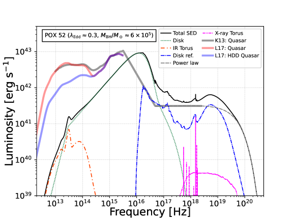
Figure 10: Model AGN SED of POX 52, composed of the thermal torus emission, the thermal and partially Comptonized disk emission, the primary X-ray power-law emission, and the X-ray reflected emission from the disk and the torus. The legend indicates their corresponding lines and colors. This SED is corrected for the dust-extinction and absorption. For comparison, a quasar SED constructed by Krawczyk et al. (2013) is plotted by a thick gray line, and two SEDs from Lyu et al. (2017) are also shown: normal-quasar SED in red and HDD-quasar SED in blue. The SED of Krawczyk et al. (2013) is adjusted from the original one so that its X-ray power-law component fits that for POX 52. On the other hand, the SEDs of Lyu et al. (2017) are re-scaled so that they smoothly connect with the SED of Krawczyk et al. (2013) at $10^{15}$ Hz.

Table 4: Data of the AGN SED and spectral components

Frequency	Total	Accretion Disk	IR Torus	X-ray Power-law	X-ray Disk Reflection	X-ray Torus
1.31e+17	7.73e+41	1.15e+41	NaN	3.09e+41	3.49e+41	3.76e+37
1.63e+17	6.08e+41	7.85e+40	NaN	3.10e+41	2.19e+41	5.67e+37
2.03e+17	5.21e+41	5.17e+40	NaN	3.11e+41	1.58e+41	9.95e+37
3.16e+17	4.49e+41	1.86e+40	NaN	3.13e+41	1.17e+41	4.63e+38
3.17e+17	4.49e+41	1.85e+40	NaN	3.13e+41	1.17e+41	4.67e+38

Note. — Frequency is in units of Hz, and the others are in units of erg s^-1. The same data are used to plot the AGN SED and spectral components in Figure 10. Luminosities below $10^{35}$ erg s^-1 are just denoted as NaN. We note that, due to this luminosity cut, the “IR Torus” values in this table are NaN, but finite values are listed in a frequency range of $\sim 10^{12}$–$10^{15}$ Hz. The entirety of this table can be obtained online.

8 Summary

POX 52 is a nearby (93 Mpc) dwarf galaxy hosting a rapidly growing low-mass AGN with $\log(M_{\rm BH}/M_{\odot})\approx 5.8$ and $\log\lambda_{\rm Edd}\approx-0.5$. This is one of the best galaxies to reveal the host and AGN properties in low-mass systems and to discuss how such an object has evolved and how its nucleus is structured. For the discussion, we collected the multi-wavelength data from the X-ray to the radio. Particularly, the X-ray data were newly obtained by the quasi-simultaneous NuSTAR and XMM-Newton observations. Our analyses and results obtained with the broadband data are summarized as follows.

• We constructed the SED from UV to IR using the XMM-Newton/OM, GALEX, PanSTARRS, 2MASS, WISE, and Spitzer/IRS data, and fitted it via the CIGALE code (Section 3). The result (Table 1) suggests that the host-galaxy has grown with the peak of SF activity being at $z\sim 1$, and the stellar light is now dominated by old stars with an accumulated mass of $M^{\rm old}_{\rm star}\approx 8.3\times 10^{8}\,M_{\odot}$. Currently, at $z\approx 0.02$, the SFR is 0.15 $M_{\odot}$ yr^-1, and the galaxy can be categorized as a star-forming galaxy.

• We decomposed the high-resolution optical HST images around 4300Å  and 8100Å into AGN and host-galaxy components using the GALFIT code (Section 4 and Figure 4), while fixing the AGN flux densities to the values constrained in the SED analysis. Then, the possible presence of a classical bulge was revealed. This was supported by the moderate bulge-to-total flux ratio of $\approx$ 0.6. Considering this ratio and the total mass, the bulge mass was estimated to be $M_{\rm bulge}\approx 5\times 10^{8}\,M_{\odot}$. Through this analysis, as a lesson learned, an unreasonable result (largely different AGN contributions in two adjacent bands) was obtained without fixing the AGN contributions, indicating the importance of simultaneous SED and image analyses.

• We have estimated the BH mass to be $\log(M_{\rm BH}/M_{\odot})\approx 5.8\pm 0.5$ by adopting the newly constrained optical AGN emission in the single-epoch method (Section 5).

• We fitted the broadband X-ray spectrum (0.2–30 keV) obtained by the quasi-simultaneous NuSTAR and XMM-Newton observations. While considering flux variation (Section 6.2) and the disk and torus components constrained in the SED analysis (Section 3), we found a reasonable X-ray model, considering thermal and Comptonized disk emission, the primary X-ray power-law emission, and the reflected emission from the disk and torus (the bottom panel of Figure 6). The BH spin parameter was roughly estimated to be $a_{\rm spin}=0.998_{-0.814}$ at a 90% confidence level (Table 3). This could suggest that most of the current mass was achieved by prolonged mass accretion.

• We have discussed a possible scenario on the evolution of POX 52. Taking past theoretical predictions into account, the presence of the bulge would suggest that POX 52 underwent a galaxy merger(s), like massive galaxies. Also, considering that POX 52 follows the $M_{\rm BH}$–$M_{\rm bulge}$ relation, observationally suggested by Schutte et al. (2019), and also the possible past prolonged accretion, a moderate AGN feedback could have taken place.

• Regarding the AGN structure, the warm coronal properties ($\tau_{\rm warm}$ and $kT_{\rm e,warm}$) are similar to those found for type-1 AGNs with larger BH masses. The primary power-law emission believed to be originating in the hot corona is soft with $\Gamma\approx 2$, consistent with what is expected from the relation with the Eddington ratio. Also, we have found that the relative strength to the bolometric luminosity ($2.2\times 10^{43}$ erg s^-1), or the 2–10 keV bolometric correction factor of $\approx$ 45, is consistent with an expected value from the Eddington-ratio dependent relation (e.g., Vasudevan & Fabian, 2007, 2009), rather than that from a luminosity-dependent one (e.g., Marconi et al., 2004; Duras et al., 2020). Finally, we have found that the geometrically thin torus constrained by the SED and X-ray data is consistent with the radiation pressure model, where the Eddington ratio is the key parameter. In summary, the corona-disk system is similar to those suggested for typical type-1 AGNs, and its nature as well as that of the torus seem to favor the Eddington-ratio-dependent scenarios. However, to explain a considerable MIR deficit found in discussing the torus emission, an additional factor may be needed. Future observations of gas and dust at wavelengths longer than far-IR will be fundamental to fully understand the observed MIR deficit.

• We have summarized the spectral data of the model AGN SED (Figure 10) in Table 4, including the data for each component. This information would be useful for discussing whether POX 52-like populations, therefore including rapidly accreting seed-BHs at high redshifts, can be detected with existing and future telescopes (e.g., JWST, NewAthena, AXIS, and LUVOIR).

We thank the reviewer for the useful comments, which helped us improve the quality of the manuscript. T.K. and S.Y. are grateful for support from RIKEN Special Postdoctoral Researcher Program. T.K., S.Y., and H.N. are supported by JSPS KAKENHI grant numbers JP23K13153, 22K20391/23K13154, and 19K21884/20KK0071/20H0941/20H01947, respectively. C.R. acknowledges support from the Fondecyt Regular grant 1230345 and ANID BASAL project FB210003. M.J.T. acknowledges support from FONDECYT Postdoctoral fellowship 3220516.

This research has made use of the NuSTAR Data Analysis Software (NuSTARDAS) jointly developed by the ASI Space Science Data Center (SSDC, Italy) and the California Institute of Technology (Caltech, USA).

This work is based on observations obtained with the ESA science mission XMM-Newton, with instruments and contributions directly funded by ESA Member States and the USA (NASA), the NuSTAR mission, a project led by the California Institute of Technology, managed by the Jet Propulsion Laboratory and funded by NASA.

This paper employs data, obtained by the Chandra X-ray Observatory, contained in  https://doi.org/10.25574/cdc.168 (catalog Chandra Data Collection (CDC) 168).

This work is based on observations made with the NASA Galaxy Evolution Explorer. GALEX is operated for NASA by the California Institute of Technology under NASA contract NAS5-9803410.17909/T9H59D (catalog (10.17909/T9H59D)).

The Pan-STARRS1 Surveys (PS1) and the PS1 public science archivedoi:10.17909/s0zg-jx37 (catalog (doi:10.17909/s0zg-jx37)) have been made possible through contributions by the Institute for Astronomy, the University of Hawaii, the Pan-STARRS Project Office, the Max-Planck Society and its participating institutes, the Max Planck Institute for Astronomy, Heidelberg and the Max Planck Institute for Extraterrestrial Physics, Garching, The Johns Hopkins University, Durham University, the University of Edinburgh, the Queen’s University Belfast, the Harvard-Smithsonian Center for Astrophysics, the Las Cumbres Observatory Global Telescope Network Incorporated, the National Central University of Taiwan, the Space Telescope Science Institute, the National Aeronautics and Space Administration under Grant No. NNX08AR22G issued through the Planetary Science Division of the NASA Science Mission Directorate, the National Science Foundation Grant No. AST-1238877, the University of Maryland, Eotvos Lorand University (ELTE), the Los Alamos National Laboratory, and the Gordon and Betty Moore Foundation.

This research is based on observations made with the NASA/ESA Hubble Space Telescope obtained from the Space Telescope Science Institute, which is operated by the Association of Universities for Research in Astronomy, Inc., under NASA contract NAS 5–26555. These observations are associated with program 10239doi:10.17909/j2ew-nh46 (catalog (doi:10.17909/j2ew-nh46)).

This publication makes use of data products from the 2MASS, which is a joint project of the University of Massachusetts and the Infrared Processing and Analysis Center/California Institute of Technology, funded by the National Aeronautics and Space Administration and the National Science Foundation.

This publication makes use of data products from the Wide-field Infrared Survey Explorer, which is a joint project of the University of California, Los Angeles, and the Jet Propulsion Laboratory/California Institute of Technology, funded by the National Aeronautics and Space Administration. This publication also makes use of data products from NEOWISE, which is a project of the Jet Propulsion Laboratory/California Institute of Technology, funded by the Planetary Science Division of the National Aeronautics and Space Administration.

This work is based in part on observations made with the Spitzer Space Telescope, which is operated by the Jet Propulsion Laboratory, California Institute of Technology under a contract with NASA. The Combined Atlas of Sources with Spitzer IRS Spectra (CASSIS) is a product of the IRS instrument team, supported by NASA and JPL. CASSIS is supported by the ”Programme National de Physique Stellaire” (PNPS) of CNRS/INSU co-funded by CEA and CNES and through the ”Programme National Physique et Chimie du Milieu Interstellaire” (PCMI) of CNRS/INSU with INC/INP co-funded by CEA and CNES.

We acknowledge the use of the NASA/IPAC Extragalactic Database (NED), which is operated by the Jet Propulsion Laboratory, California Institute of Technology, under contract with the National Aeronautics and Space Administration.

This work has also made use of the VizieR catalogue access tool, CDS, Strasbourg, France.

References

- Allen et al. (2006) Allen, P. D., Driver, S. P., Graham, A. W., et al. 2006, MNRAS, 371, 2, doi: 10.1111/j.1365-2966.2006.10586.x
- Arnaud (1996) Arnaud, K. A. 1996, Astronomical Society of the Pacific Conference Series, Vol. 101, XSPEC: The First Ten Years, ed. G. H. Jacoby & J. Barnes, 17
- Asmus et al. (2015) Asmus, D., Gandhi, P., Hönig, S. F., Smette, A., & Duschl, W. J. 2015, MNRAS, 454, 766, doi: 10.1093/mnras/stv1950
- Astropy Collaboration et al. (2013) Astropy Collaboration, Robitaille, T. P., Tollerud, E. J., et al. 2013, A&A, 558, A33, doi: 10.1051/0004-6361/201322068
- Astropy Collaboration et al. (2018) Astropy Collaboration, Price-Whelan, A. M., Sipőcz, B. M., et al. 2018, AJ, 156, 123, doi: 10.3847/1538-3881/aabc4f
- Bañados et al. (2018) Bañados, E., Venemans, B. P., Mazzucchelli, C., et al. 2018, Nature, 553, 473, doi: 10.1038/nature25180
- Baldassare et al. (2020) Baldassare, V. F., Geha, M., & Greene, J. 2020, ApJ, 896, 10, doi: 10.3847/1538-4357/ab8936
- Barth et al. (2004) Barth, A. J., Ho, L. C., Rutledge, R. E., & Sargent, W. L. W. 2004, ApJ, 607, 90, doi: 10.1086/383302
- Bellovary et al. (2019) Bellovary, J. M., Cleary, C. E., Munshi, F., et al. 2019, MNRAS, 482, 2913, doi: 10.1093/mnras/sty2842
- Bentz et al. (2006) Bentz, M. C., Peterson, B. M., Pogge, R. W., Vestergaard, M., & Onken, C. A. 2006, ApJ, 644, 133, doi: 10.1086/503537
- Berti & Volonteri (2008) Berti, E., & Volonteri, M. 2008, ApJ, 684, 822, doi: 10.1086/590379
- Bianchi et al. (2017) Bianchi, L., Shiao, B., & Thilker, D. 2017, ApJS, 230, 24, doi: 10.3847/1538-4365/aa7053
- Bianchi et al. (2009) Bianchi, S., Guainazzi, M., Matt, G., Fonseca Bonilla, N., & Ponti, G. 2009, A&A, 495, 421, doi: 10.1051/0004-6361:200810620
- Boissay et al. (2016) Boissay, R., Ricci, C., & Paltani, S. 2016, A&A, 588, A70, doi: 10.1051/0004-6361/201526982
- Booth & Schaye (2009) Booth, C. M., & Schaye, J. 2009, MNRAS, 398, 53, doi: 10.1111/j.1365-2966.2009.15043.x
- Boquien et al. (2019) Boquien, M., Burgarella, D., Roehlly, Y., et al. 2019, A&A, 622, A103, doi: 10.1051/0004-6361/201834156
- Boylan-Kolchin et al. (2011) Boylan-Kolchin, M., Bullock, J. S., & Kaplinghat, M. 2011, MNRAS, 415, L40, doi: 10.1111/j.1745-3933.2011.01074.x
- Bruzual & Charlot (2003) Bruzual, G., & Charlot, S. 2003, MNRAS, 344, 1000, doi: 10.1046/j.1365-8711.2003.06897.x
- Buat et al. (2018) Buat, V., Boquien, M., Małek, K., et al. 2018, A&A, 619, A135, doi: 10.1051/0004-6361/201833841
- Buat et al. (2021) Buat, V., Mountrichas, G., Yang, G., et al. 2021, A&A, 654, A93, doi: 10.1051/0004-6361/202141797
- Campitiello et al. (2021) Campitiello, S., Celotti, A., Ghisellini, G., & Sbarrato, T. 2021, A&A, 656, A96, doi: 10.1051/0004-6361/202141602
- Cardelli et al. (1989) Cardelli, J. A., Clayton, G. C., & Mathis, J. S. 1989, ApJ, 345, 245, doi: 10.1086/167900
- Cash (1979) Cash, W. 1979, ApJ, 228, 939, doi: 10.1086/156922
- Chabrier (2003) Chabrier, G. 2003, PASP, 115, 763, doi: 10.1086/376392
- Chadayammuri et al. (2023) Chadayammuri, U., Bogdán, Á., Ricarte, A., & Natarajan, P. 2023, ApJ, 946, 51, doi: 10.3847/1538-4357/acbea6
- Chambers et al. (2016) Chambers, K. C., Magnier, E. A., Metcalfe, N., et al. 2016, arXiv e-prints, arXiv:1612.05560, doi: 10.48550/arXiv.1612.05560
- Charlot & Fall (2000) Charlot, S., & Fall, S. M. 2000, ApJ, 539, 718, doi: 10.1086/309250
- Ciesla et al. (2015) Ciesla, L., Charmandaris, V., Georgakakis, A., et al. 2015, A&A, 576, A10, doi: 10.1051/0004-6361/201425252
- Ciesla et al. (2016) Ciesla, L., Boselli, A., Elbaz, D., et al. 2016, A&A, 585, A43, doi: 10.1051/0004-6361/201527107
- Croton et al. (2006) Croton, D. J., Springel, V., White, S. D. M., et al. 2006, MNRAS, 365, 11, doi: 10.1111/j.1365-2966.2005.09675.x
- Crummy et al. (2006) Crummy, J., Fabian, A. C., Gallo, L., & Ross, R. R. 2006, MNRAS, 365, 1067, doi: 10.1111/j.1365-2966.2005.09844.x
- Cruz et al. (2023) Cruz, H. A. G., Goulding, A. D., & Greene, J. E. 2023, arXiv e-prints, arXiv:2307.15111, doi: 10.48550/arXiv.2307.15111
- Dashyan et al. (2018) Dashyan, G., Silk, J., Mamon, G. A., Dubois, Y., & Hartwig, T. 2018, MNRAS, 473, 5698, doi: 10.1093/mnras/stx2716
- Dauser et al. (2014) Dauser, T., Garcia, J., Parker, M. L., Fabian, A. C., & Wilms, J. 2014, MNRAS, 444, L100, doi: 10.1093/mnrasl/slu125
- Dauser et al. (2013) Dauser, T., Garcia, J., Wilms, J., et al. 2013, MNRAS, 430, 1694, doi: 10.1093/mnras/sts710
- de Blok (2010) de Blok, W. J. G. 2010, Advances in Astronomy, 2010, 789293, doi: 10.1155/2010/789293
- Di Matteo et al. (2005) Di Matteo, T., Springel, V., & Hernquist, L. 2005, Nature, 433, 604, doi: 10.1038/nature03335
- Done et al. (2012) Done, C., Davis, S. W., Jin, C., Blaes, O., & Ward, M. 2012, MNRAS, 420, 1848, doi: 10.1111/j.1365-2966.2011.19779.x
- Draine (2003) Draine, B. T. 2003, ARA&A, 41, 241, doi: 10.1146/annurev.astro.41.011802.094840
- Draine & Li (2007) Draine, B. T., & Li, A. 2007, ApJ, 657, 810, doi: 10.1086/511055
- Draine et al. (2014) Draine, B. T., Aniano, G., Krause, O., et al. 2014, ApJ, 780, 172, doi: 10.1088/0004-637X/780/2/172
- Duras et al. (2020) Duras, F., Bongiorno, A., Ricci, F., et al. 2020, A&A, 636, A73, doi: 10.1051/0004-6361/201936817
- Efstathiou (1992) Efstathiou, G. 1992, MNRAS, 256, 43P, doi: 10.1093/mnras/256.1.43P
- Fabian (2012) Fabian, A. C. 2012, ARA&A, 50, 455, doi: 10.1146/annurev-astro-081811-125521
- Fabian et al. (2008) Fabian, A. C., Vasudevan, R. V., & Gandhi, P. 2008, MNRAS, 385, L43, doi: 10.1111/j.1745-3933.2008.00430.x
- Fabian et al. (2009) Fabian, A. C., Vasudevan, R. V., Mushotzky, R. F., Winter, L. M., & Reynolds, C. S. 2009, MNRAS, 394, L89, doi: 10.1111/j.1745-3933.2009.00617.x
- Fitts et al. (2017) Fitts, A., Boylan-Kolchin, M., Elbert, O. D., et al. 2017, MNRAS, 471, 3547, doi: 10.1093/mnras/stx1757
- Flewelling et al. (2020) Flewelling, H. A., Magnier, E. A., Chambers, K. C., et al. 2020, ApJS, 251, 7, doi: 10.3847/1538-4365/abb82d
- Floyd et al. (2008) Floyd, D. J. E., Axon, D., Baum, S., et al. 2008, ApJS, 177, 148, doi: 10.1086/587622
- Fruscione et al. (2006) Fruscione, A., McDowell, J. C., Allen, G. E., et al. 2006, in Society of Photo-Optical Instrumentation Engineers (SPIE) Conference Series, Vol. 6270, Society of Photo-Optical Instrumentation Engineers (SPIE) Conference Series, ed. D. R. Silva & R. E. Doxsey, 62701V, doi: 10.1117/12.671760
- Gabriel et al. (2004) Gabriel, C., Denby, M., Fyfe, D. J., et al. 2004, in Astronomical Society of the Pacific Conference Series, Vol. 314, Astronomical Data Analysis Software and Systems (ADASS) XIII, ed. F. Ochsenbein, M. G. Allen, & D. Egret, 759
- Gandhi et al. (2009) Gandhi, P., Horst, H., Smette, A., et al. 2009, A&A, 502, 457, doi: 10.1051/0004-6361/200811368
- Gao et al. (2022) Gao, H., Ho, L. C., & Li, Z.-Y. 2022, ApJS, 262, 54, doi: 10.3847/1538-4365/ac8dea
- García et al. (2014) García, J., Dauser, T., Lohfink, A., et al. 2014, ApJ, 782, 76, doi: 10.1088/0004-637X/782/2/76
- Gebhardt et al. (2000) Gebhardt, K., Bender, R., Bower, G., et al. 2000, ApJ, 539, L13, doi: 10.1086/312840
- Gordon et al. (2020) Gordon, Y. A., Boyce, M. M., O’Dea, C. P., et al. 2020, Research Notes of the American Astronomical Society, 4, 175, doi: 10.3847/2515-5172/abbe23
- Gordon et al. (2021) —. 2021, ApJS, 255, 30, doi: 10.3847/1538-4365/ac05c0
- Greene (2012) Greene, J. E. 2012, Nature Communications, 3, 1304, doi: 10.1038/ncomms2314
- Greene & Ho (2004) Greene, J. E., & Ho, L. C. 2004, ApJ, 610, 722, doi: 10.1086/421719
- Greene & Ho (2005) —. 2005, ApJ, 630, 122, doi: 10.1086/431897
- Greene & Ho (2007) —. 2007, ApJ, 670, 92, doi: 10.1086/522082
- Greene et al. (2020) Greene, J. E., Strader, J., & Ho, L. C. 2020, ARA&A, 58, 257, doi: 10.1146/annurev-astro-032620-021835
- Griffin et al. (2020) Griffin, A. J., Lacey, C. G., Gonzalez-Perez, V., et al. 2020, MNRAS, 492, 2535, doi: 10.1093/mnras/staa024
- Gültekin et al. (2009) Gültekin, K., Richstone, D. O., Gebhardt, K., et al. 2009, ApJ, 698, 198, doi: 10.1088/0004-637X/698/1/198
- Hao et al. (2010) Hao, H., Elvis, M., Civano, F., et al. 2010, ApJ, 724, L59, doi: 10.1088/2041-8205/724/1/L59
- Harris et al. (2020) Harris, C. R., Millman, K. J., van der Walt, S. J., et al. 2020, Nature, 585, 357, doi: 10.1038/s41586-020-2649-2
- Harrison et al. (2018) Harrison, C. M., Costa, T., Tadhunter, C. N., et al. 2018, Nature Astronomy, 2, 198, doi: 10.1038/s41550-018-0403-6
- Harrison et al. (2013) Harrison, F. A., Craig, W. W., Christensen, F. E., et al. 2013, ApJ, 770, 103, doi: 10.1088/0004-637X/770/2/103
- Hood et al. (2017) Hood, C. E., Barth, A. J., Ho, L. C., & Greene, J. E. 2017, ApJ, 838, 26, doi: 10.3847/1538-4357/aa60c9
- Hopkins et al. (2008) Hopkins, P. F., Hernquist, L., Cox, T. J., & Kereš, D. 2008, ApJS, 175, 356, doi: 10.1086/524362
- Hopkins & Quataert (2010) Hopkins, P. F., & Quataert, E. 2010, MNRAS, 407, 1529, doi: 10.1111/j.1365-2966.2010.17064.x
- Hopkins et al. (2010) Hopkins, P. F., Bundy, K., Croton, D., et al. 2010, ApJ, 715, 202, doi: 10.1088/0004-637X/715/1/202
- Hunter (2007) Hunter, J. D. 2007, Computing in Science and Engineering, 9, 90, doi: 10.1109/MCSE.2007.55
- Ichikawa et al. (2017) Ichikawa, K., Ricci, C., Ueda, Y., et al. 2017, ApJ, 835, 74, doi: 10.3847/1538-4357/835/1/74
- Inoue (2011) Inoue, A. K. 2011, MNRAS, 415, 2920, doi: 10.1111/j.1365-2966.2011.18906.x
- Izumi et al. (2016) Izumi, T., Kawakatu, N., & Kohno, K. 2016, ApJ, 827, 81, doi: 10.3847/0004-637X/827/1/81
- Jansen et al. (2001) Jansen, F., Lumb, D., Altieri, B., et al. 2001, A&A, 365, L1, doi: 10.1051/0004-6361:20000036
- Jiang et al. (2020) Jiang, J., Gallo, L. C., Fabian, A. C., Parker, M. L., & Reynolds, C. S. 2020, MNRAS, 498, 3888, doi: 10.1093/mnras/staa2625
- Jiang et al. (2010) Jiang, L., Fan, X., Brandt, W. N., et al. 2010, Nature, 464, 380, doi: 10.1038/nature08877
- Jin et al. (2012) Jin, C., Ward, M., Done, C., & Gelbord, J. 2012, MNRAS, 420, 1825, doi: 10.1111/j.1365-2966.2011.19805.x
- Kalberla et al. (2005) Kalberla, P. M. W., Burton, W. B., Hartmann, D., et al. 2005, A&A, 440, 775, doi: 10.1051/0004-6361:20041864
- Kammoun et al. (2015) Kammoun, E. S., Papadakis, I. E., & Sabra, B. M. 2015, A&A, 582, A40, doi: 10.1051/0004-6361/201526811
- Kawamuro et al. (2021) Kawamuro, T., Ricci, C., Izumi, T., et al. 2021, ApJS, 257, 64, doi: 10.3847/1538-4365/ac2891
- Kawamuro et al. (2016) Kawamuro, T., Ueda, Y., Tazaki, F., Ricci, C., & Terashima, Y. 2016, ApJS, 225, 14, doi: 10.3847/0067-0049/225/1/14
- Kennicutt & Evans (2012) Kennicutt, R. C., & Evans, N. J. 2012, ARA&A, 50, 531, doi: 10.1146/annurev-astro-081811-125610
- King & Pounds (2015) King, A., & Pounds, K. 2015, ARA&A, 53, 115, doi: 10.1146/annurev-astro-082214-122316
- Kokubo & Minezaki (2020) Kokubo, M., & Minezaki, T. 2020, MNRAS, 491, 4615, doi: 10.1093/mnras/stz3397
- Kormendy & Ho (2013) Kormendy, J., & Ho, L. C. 2013, ARA&A, 51, 511, doi: 10.1146/annurev-astro-082708-101811
- Koudmani et al. (2021) Koudmani, S., Henden, N. A., & Sijacki, D. 2021, MNRAS, 503, 3568, doi: 10.1093/mnras/stab677
- Koudmani et al. (2019) Koudmani, S., Sijacki, D., Bourne, M. A., & Smith, M. C. 2019, MNRAS, 484, 2047, doi: 10.1093/mnras/stz097
- Koudmani et al. (2022) Koudmani, S., Sijacki, D., & Smith, M. C. 2022, MNRAS, 516, 2112, doi: 10.1093/mnras/stac2252
- Krawczyk et al. (2013) Krawczyk, C. M., Richards, G. T., Mehta, S. S., et al. 2013, ApJS, 206, 4, doi: 10.1088/0067-0049/206/1/4
- Krist et al. (2011) Krist, J. E., Hook, R. N., & Stoehr, F. 2011, in Society of Photo-Optical Instrumentation Engineers (SPIE) Conference Series, Vol. 8127, Optical Modeling and Performance Predictions V, ed. M. A. Kahan, 81270J, doi: 10.1117/12.892762
- Kroupa et al. (2005) Kroupa, P., Theis, C., & Boily, C. M. 2005, A&A, 431, 517, doi: 10.1051/0004-6361:20041122
- Kubota & Done (2018) Kubota, A., & Done, C. 2018, MNRAS, 480, 1247, doi: 10.1093/mnras/sty1890
- Kubota et al. (1998) Kubota, A., Tanaka, Y., Makishima, K., et al. 1998, PASJ, 50, 667, doi: 10.1093/pasj/50.6.667
- Kunth et al. (1981) Kunth, D., Sargent, W. L. W., & Kowal, C. 1981, A&AS, 44, 229
- Larson (1974) Larson, R. B. 1974, MNRAS, 169, 229, doi: 10.1093/mnras/169.2.229
- Lebouteiller et al. (2015) Lebouteiller, V., Barry, D. J., Goes, C., et al. 2015, ApJS, 218, 21, doi: 10.1088/0067-0049/218/2/21
- Lebouteiller et al. (2011) Lebouteiller, V., Barry, D. J., Spoon, H. W. W., et al. 2011, ApJS, 196, 8, doi: 10.1088/0067-0049/196/1/8
- Lewin et al. (2022) Lewin, C., Kara, E., Wilkins, D., et al. 2022, ApJ, 939, 109, doi: 10.3847/1538-4357/ac978f
- Liu et al. (2020) Liu, W., Veilleux, S., Canalizo, G., et al. 2020, ApJ, 905, 166, doi: 10.3847/1538-4357/abc269
- Lyu et al. (2017) Lyu, J., Rieke, G. H., & Shi, Y. 2017, ApJ, 835, 257, doi: 10.3847/1538-4357/835/2/257
- Magorrian et al. (1998) Magorrian, J., Tremaine, S., Richstone, D., et al. 1998, AJ, 115, 2285, doi: 10.1086/300353
- Mainzer et al. (2011) Mainzer, A., Bauer, J., Grav, T., et al. 2011, ApJ, 731, 53, doi: 10.1088/0004-637X/731/1/53
- Mallick et al. (2022) Mallick, L., Fabian, A. C., García, J. A., et al. 2022, MNRAS, 513, 4361, doi: 10.1093/mnras/stac990
- Manzano-King et al. (2019) Manzano-King, C. M., Canalizo, G., & Sales, L. V. 2019, ApJ, 884, 54, doi: 10.3847/1538-4357/ab4197
- Marchesi et al. (2020) Marchesi, S., Gilli, R., Lanzuisi, G., et al. 2020, A&A, 642, A184, doi: 10.1051/0004-6361/202038622
- Marconi & Hunt (2003) Marconi, A., & Hunt, L. K. 2003, ApJ, 589, L21, doi: 10.1086/375804
- Marconi et al. (2004) Marconi, A., Risaliti, G., Gilli, R., et al. 2004, MNRAS, 351, 169, doi: 10.1111/j.1365-2966.2004.07765.x
- Marleau et al. (2017) Marleau, F. R., Clancy, D., Habas, R., & Bianconi, M. 2017, A&A, 602, A28, doi: 10.1051/0004-6361/201629832
- Martin et al. (2005) Martin, D. C., Fanson, J., Schiminovich, D., et al. 2005, ApJ, 619, L1, doi: 10.1086/426387
- McMullin et al. (2007) McMullin, J. P., Waters, B., Schiebel, D., Young, W., & Golap, K. 2007, Astronomical Society of the Pacific Conference Series, Vol. 376, CASA Architecture and Applications, ed. R. A. Shaw, F. Hill, & D. J. Bell, 127
- Meert et al. (2015) Meert, A., Vikram, V., & Bernardi, M. 2015, MNRAS, 446, 3943, doi: 10.1093/mnras/stu2333
- Mendel et al. (2014) Mendel, J. T., Simard, L., Palmer, M., Ellison, S. L., & Patton, D. R. 2014, ApJS, 210, 3, doi: 10.1088/0067-0049/210/1/3
- Mezcua (2017) Mezcua, M. 2017, International Journal of Modern Physics D, 26, 1730021, doi: 10.1142/S021827181730021X
- Mezcua & Domínguez Sánchez (2020) Mezcua, M., & Domínguez Sánchez, H. 2020, ApJ, 898, L30, doi: 10.3847/2041-8213/aba199
- Middei et al. (2020) Middei, R., Petrucci, P. O., Bianchi, S., et al. 2020, A&A, 640, A99, doi: 10.1051/0004-6361/202038112
- Miller et al. (2015) Miller, B. P., Gallo, E., Greene, J. E., et al. 2015, ApJ, 799, 98, doi: 10.1088/0004-637X/799/1/98
- Mitsuda et al. (1984) Mitsuda, K., Inoue, H., Koyama, K., et al. 1984, PASJ, 36, 741
- Miyaji et al. (2019) Miyaji, T., Herrera-Endoqui, M., Krumpe, M., et al. 2019, ApJ, 884, L10, doi: 10.3847/2041-8213/ab46bc
- Monje et al. (2011) Monje, R. R., Blain, A. W., & Phillips, T. G. 2011, ApJS, 195, 23, doi: 10.1088/0067-0049/195/2/23
- Moore et al. (1999) Moore, B., Ghigna, S., Governato, F., et al. 1999, ApJ, 524, L19, doi: 10.1086/312287
- Naab & Burkert (2003) Naab, T., & Burkert, A. 2003, ApJ, 597, 893, doi: 10.1086/378581
- Nenkova et al. (2008a) Nenkova, M., Sirocky, M. M., Ivezić, Ž., & Elitzur, M. 2008a, ApJ, 685, 147, doi: 10.1086/590482
- Nenkova et al. (2008b) Nenkova, M., Sirocky, M. M., Nikutta, R., Ivezić, Ž., & Elitzur, M. 2008b, ApJ, 685, 160, doi: 10.1086/590483
- Noda et al. (2013a) Noda, H., Makishima, K., Nakazawa, K., et al. 2013a, PASJ, 65, 4, doi: 10.1093/pasj/65.1.4
- Noda et al. (2013b) Noda, H., Makishima, K., Nakazawa, K., & Yamada, S. 2013b, ApJ, 771, 100, doi: 10.1088/0004-637X/771/2/100
- Noda et al. (2014) Noda, H., Makishima, K., Yamada, S., et al. 2014, ApJ, 794, 2, doi: 10.1088/0004-637X/794/1/2
- Noda et al. (2011) —. 2011, PASJ, 63, S925, doi: 10.1093/pasj/63.sp3.S925
- Onken et al. (2004) Onken, C. A., Ferrarese, L., Merritt, D., et al. 2004, ApJ, 615, 645, doi: 10.1086/424655
- Onoue et al. (2019) Onoue, M., Kashikawa, N., Matsuoka, Y., et al. 2019, ApJ, 880, 77, doi: 10.3847/1538-4357/ab29e9
- Panessa et al. (2015) Panessa, F., Tarchi, A., Castangia, P., et al. 2015, MNRAS, 447, 1289, doi: 10.1093/mnras/stu2455
- Peng et al. (2002) Peng, C. Y., Ho, L. C., Impey, C. D., & Rix, H.-W. 2002, AJ, 124, 266, doi: 10.1086/340952
- Peng et al. (2010) —. 2010, AJ, 139, 2097, doi: 10.1088/0004-6256/139/6/2097
- Penny et al. (2018) Penny, S. J., Masters, K. L., Smethurst, R., et al. 2018, MNRAS, 476, 979, doi: 10.1093/mnras/sty202
- Petrucci et al. (2018) Petrucci, P. O., Ursini, F., De Rosa, A., et al. 2018, A&A, 611, A59, doi: 10.1051/0004-6361/201731580
- Petrucci et al. (2013) Petrucci, P. O., Paltani, S., Malzac, J., et al. 2013, A&A, 549, A73, doi: 10.1051/0004-6361/201219956
- Ricci et al. (2017a) Ricci, C., Trakhtenbrot, B., Koss, M. J., et al. 2017a, ApJS, 233, 17, doi: 10.3847/1538-4365/aa96ad
- Ricci et al. (2017b) —. 2017b, Nature, 549, 488, doi: 10.1038/nature23906
- Ricci et al. (2018) Ricci, C., Ho, L. C., Fabian, A. C., et al. 2018, MNRAS, 480, 1819, doi: 10.1093/mnras/sty1879
- Ricci et al. (2022) Ricci, F., Treister, E., Bauer, F. E., et al. 2022, ApJS, 261, 8, doi: 10.3847/1538-4365/ac5b67
- Ross & Fabian (2005) Ross, R. R., & Fabian, A. C. 2005, MNRAS, 358, 211, doi: 10.1111/j.1365-2966.2005.08797.x
- Salpeter (1964) Salpeter, E. E. 1964, ApJ, 140, 796, doi: 10.1086/147973
- Schartmann et al. (2005) Schartmann, M., Meisenheimer, K., Camenzind, M., Wolf, S., & Henning, T. 2005, A&A, 437, 861, doi: 10.1051/0004-6361:20042363
- Schutte et al. (2019) Schutte, Z., Reines, A. E., & Greene, J. E. 2019, ApJ, 887, 245, doi: 10.3847/1538-4357/ab35dd
- Shakura & Sunyaev (1973) Shakura, N. I., & Sunyaev, R. A. 1973, A&A, 24, 337
- Shangguan et al. (2020) Shangguan, J., Ho, L. C., Bauer, F. E., Wang, R., & Treister, E. 2020, ApJ, 899, 112, doi: 10.3847/1538-4357/aba8a1
- Sharma et al. (2022) Sharma, R. S., Brooks, A. M., Tremmel, M., et al. 2022, ApJ, 936, 82, doi: 10.3847/1538-4357/ac8664
- Shemmer et al. (2006) Shemmer, O., Brandt, W. N., Netzer, H., Maiolino, R., & Kaspi, S. 2006, ApJ, 646, L29, doi: 10.1086/506911
- Shemmer et al. (2008) —. 2008, ApJ, 682, 81, doi: 10.1086/588776
- Silk (2017) Silk, J. 2017, ApJ, 839, L13, doi: 10.3847/2041-8213/aa67da
- Skrutskie et al. (2006) Skrutskie, M. F., Cutri, R. M., Stiening, R., et al. 2006, AJ, 131, 1163, doi: 10.1086/498708
- Spoon et al. (2022) Spoon, H. W. W., Hernán-Caballero, A., Rupke, D., et al. 2022, ApJS, 259, 37, doi: 10.3847/1538-4365/ac4989
- Stalevski et al. (2016) Stalevski, M., Ricci, C., Ueda, Y., et al. 2016, MNRAS, 458, 2288, doi: 10.1093/mnras/stw444
- Tabatabaei et al. (2017) Tabatabaei, F. S., Schinnerer, E., Krause, M., et al. 2017, ApJ, 836, 185, doi: 10.3847/1538-4357/836/2/185
- Tanimoto et al. (2019) Tanimoto, A., Ueda, Y., Odaka, H., et al. 2019, ApJ, 877, 95, doi: 10.3847/1538-4357/ab1b20
- Team (2023) Team, T. P. D. 2023, pandas-dev/pandas: Pandas, v2.1.1, Zenodo, Zenodo, doi: 10.5281/zenodo.3509134
- Thorne (1974) Thorne, K. S. 1974, ApJ, 191, 507, doi: 10.1086/152991
- Thornton et al. (2008) Thornton, C. E., Barth, A. J., Ho, L. C., Rutledge, R. E., & Greene, J. E. 2008, ApJ, 686, 892, doi: 10.1086/591519
- Toba et al. (2021) Toba, Y., Ueda, Y., Gandhi, P., et al. 2021, ApJ, 912, 91, doi: 10.3847/1538-4357/abe94a
- Trakhtenbrot et al. (2017) Trakhtenbrot, B., Ricci, C., Koss, M. J., et al. 2017, MNRAS, 470, 800, doi: 10.1093/mnras/stx1117
- Trebitsch et al. (2018) Trebitsch, M., Volonteri, M., Dubois, Y., & Madau, P. 2018, MNRAS, 478, 5607, doi: 10.1093/mnras/sty1406
- Valiante et al. (2018) Valiante, R., Schneider, R., Zappacosta, L., et al. 2018, MNRAS, 476, 407, doi: 10.1093/mnras/sty213
- Vasudevan & Fabian (2007) Vasudevan, R. V., & Fabian, A. C. 2007, MNRAS, 381, 1235, doi: 10.1111/j.1365-2966.2007.12328.x
- Vasudevan & Fabian (2009) —. 2009, MNRAS, 392, 1124, doi: 10.1111/j.1365-2966.2008.14108.x
- Vaughan et al. (2003) Vaughan, S., Edelson, R., Warwick, R. S., & Uttley, P. 2003, MNRAS, 345, 1271, doi: 10.1046/j.1365-2966.2003.07042.x
- Vestergaard (2002) Vestergaard, M. 2002, ApJ, 571, 733, doi: 10.1086/340045
- Vestergaard & Peterson (2006) Vestergaard, M., & Peterson, B. M. 2006, ApJ, 641, 689, doi: 10.1086/500572
- Virtanen et al. (2020) Virtanen, P., Gommers, R., Oliphant, T. E., et al. 2020, Nature Methods, 17, 261, doi: 10.1038/s41592-019-0686-2
- Vogelsberger et al. (2013) Vogelsberger, M., Genel, S., Sijacki, D., et al. 2013, MNRAS, 436, 3031, doi: 10.1093/mnras/stt1789
- Volonteri et al. (2005) Volonteri, M., Madau, P., Quataert, E., & Rees, M. J. 2005, ApJ, 620, 69, doi: 10.1086/426858
- Whitaker et al. (2012) Whitaker, K. E., van Dokkum, P. G., Brammer, G., & Franx, M. 2012, ApJ, 754, L29, doi: 10.1088/2041-8205/754/2/L29
- Wright et al. (2010) Wright, E. L., Eisenhardt, P. R. M., Mainzer, A. K., et al. 2010, AJ, 140, 1868, doi: 10.1088/0004-6256/140/6/1868
- Wu et al. (2015) Wu, X.-B., Wang, F., Fan, X., et al. 2015, Nature, 518, 512, doi: 10.1038/nature14241
- Xu et al. (2021) Xu, Y., García, J. A., Walton, D. J., et al. 2021, ApJ, 913, 13, doi: 10.3847/1538-4357/abf430
- Yamada et al. (2023) Yamada, S., Ueda, Y., Herrera-Endoqui, M., et al. 2023, ApJS, 265, 37, doi: 10.3847/1538-4365/acb349
- Yamada (1994) Yamada, T. 1994, ApJ, 423, L27, doi: 10.1086/187227
- Yang et al. (2020) Yang, G., Boquien, M., Buat, V., et al. 2020, MNRAS, 491, 740, doi: 10.1093/mnras/stz3001