SolarFormer: Multi-scale Transformer for Solar PV Profiling
††thanks: This material is based upon work supported by the National Science Foundation (NSF) under Award OIA-1946391 RII Track-1, NSF 2119691 AI SUSTEIN, NSF 2236302
Abstract
As climate change intensifies, the global imperative to shift towards sustainable energy sources becomes more pronounced. Photovoltaic (PV) energy is a favored choice due to its reliability and ease of installation. Accurate mapping of PV installations is crucial for understanding their adoption and informing energy policy. To meet this need, we introduce the SolarFormer, designed to segment solar panels from aerial imagery, offering insights into their location and size. However, solar panel identification in Computer Vision is intricate due to various factors like weather conditions, roof conditions, and Ground Sampling Distance (GSD) variations. To tackle these complexities, we present the SolarFormer, featuring a multi-scale Transformer encoder and a masked-attention Transformer decoder. Our model leverages low-level features and incorporates an instance query mechanism to enhance the localization of solar PV installations. We rigorously evaluated our SolarFormer using diverse datasets, including GGE (France), IGN (France), and USGS (California, USA), across different GSDs. Our extensive experiments consistently demonstrate that our model either matches or surpasses state-of-the-art models, promising enhanced solar panel segmentation for global sustainable energy initiatives. Source code is available upon acceptance.
Index Terms:
Aerial Images, Solar PVs, Profiling, Segmentation, multi-scale, Transformers.I Introduction
The growth of photovoltaic (PV) energy production has been impressive, driven by improved cell manufacturing [1], a competitive market, and increasing energy costs [2]. In 2022, the U.S. Energy Information Administration reported a 440% increase in small-scale PV installation capacity, reaching 39.5 GW from 7.3 GW in 2014 [3].
While solar panels offer sustainability, they pose challenges for energy forecasting [4]. PV energy relies on weather conditions, operates in decentralized systems, and often remains unseen by Transmission System Operators [5]. Accurate forecasting is crucial, especially in high PV adoption areas, to prevent grid congestion and imbalances [4].
To gain real-time insights into PV distribution and energy production, recent research has focused on profiling PV installations using remote sensing imagery from unmanned vehicles [6] and satellites, coupled with Machine Learning and Computer Vision. Remote Sensing (RS) images provide an overhead view of the Earth’s surface and define the level of detail as Ground Sample Distance (GSD). RS imagery serves multiple practical purposes, including climate change analysis [7], natural disaster monitoring [8], urban planning [9][10], and land cover analysis [11].
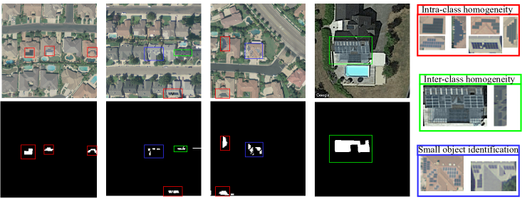
Deep Learning (DL) has achieved remarkable image understanding capabilities, even surpassing human performance. DL has been applied to extract solar PV distribution through a two-step process: training a classifier to identify images with solar panels and passing them to the segmentation network such as Kasmi, et al., [12], HyperionSolarNet[13]. However, existing DL-based methods have two major limitations: (i) They employ a two-stage framework, consisting of separate classifier and segmentor networks. This approach heavily relies on the classifier network, leading to suboptimal learning in the segmentation network. Essentially, they adapt existing DL frameworks designed for natural images to solar PV imagery, neglecting the unique challenges posed by the latter. (ii) These existing DL frameworks are originally designed for natural images and do not adequately address the specific challenges encountered in solar PV imagery. As depicted in Fig.1, these challenges include intra-class heterogeneity, inter-class homogeneity, and the identification of small objects.
To overcome these limitations, we have harnessed recent advances in Deep Learning, particularly the Transformer architecture [14], to introduce a novel model called SolarFormer. Our SolarFormer incorporates a multi-scale Transformer encoder and a masked-attention Transformer decoder to address these challenges effectively. Our contributions can be summarized as follows:
-
•
Implementation of a high-resolution Transformer to enhance solar PV understanding, particularly in cases with low resolution and GSD variations.
-
•
Deployment of a multi-scale Transformer encoder with a masked-attention Transformer decoder to extract rich visual representations, effectively addressing inter-class and intra-class homogeneity challenges.
-
•
An extensive comparative evaluation between our SolarFormer and existing DL models using three public datasets, demonstrating the effectiveness of our proposed approach.
II Related Works
II-A Deep Learning-based Solar PV Analysis
In recent times, the mapping of high-fidelity solar installations has become increasingly important. This uptick in interest is a direct result of the rapid adoption of photovoltaic (PV) energy, enhanced resolution of aerial imagery, and the advancements in DL techniques. The preliminary efforts in this field focused on binary classification of images, determining the presence or absence of PV installations [15] [16].
DeepSolar [6] utilizes a Convolutional Neural Network (CNN) as a dual-stage network which includes classification and segmentation strategy, marked a significant milestone in solar PV profiling. The success of this endeavor paved the way for refining the characterization network. This was achieved by integrating state-of-the-art (SOTA) CNN methods into classifier and segmentation architectures. Meanwhile, certain researchers opted to concentrate solely on segmentation such as Zhuang, et al., [17], Zech, et al., [18]. Furthermore, these methodologies are adaptable for generating PV capacity estimates 3D-PV-Locator[19], Kasmi, et al., [12] and conducting socioeconomic analyses such as DeepSolar [6]. Such assessments leverage the dimensions and geographical data of the segmented installations
A prominent challenge is the creation of suitable datasets. The complications arise from (i) the extensive need for annotated images, a process that’s both time-consuming and meticulous, and (ii) the potential sensitivity of the data, making it unsuitable for public distribution. Fortunately, organizations like IGN and USGS have been proactive, offering freely accessible aerial images. Despite this support, researchers often find themselves in a bind — they either annotate a limited selection of aerial imagery such as Hyperion-Solar-Net[13], keep the collected data unreleased or organize crowd sourced annotating campaigns such as IGN-France [20], USGS, California [21].
II-B Transformer
Transformer [14] and Vision Transformer (ViT) [22] have recently attracted significant interest in the research community. Initially implemented for Natural Language Processing (NLP) tasks, the Transformer [14] incorporates a self-attention mechanism to enhance learning on long-range relationships inside the data. It also can be adapted for parallelization, allowing for faster training on multiple nodes for large datasets. This capabilities have proven very useful for multiple NLP tasks [23]. The ViT divides a 2D image into patches and then feeds the 1D sequence of linear embedding into the Transformer in a similar manner as how words would be treated for a NLP Transformer. This scheme proved specially useful when dealing with large datasets, where the ViT was able to attend to the information from the lowest levels and produce better global context than CNNs. This novel approach has already been implemented for a variety of tasks such as image recognition [24, 25], video captioning [26] [27], action localization [28, 29], aerial imaging [12] object detection [30, 31] and image segmentation [31], medical imaging [32] proving their capacity to synthesise global information.
Presently, most DL-based methods for solar PV analysis are merely adaptations of pre-existing DL techniques tailored for solar PV data. Consequently, they frequently fail to tackle unique challenges inherent to solar PV datasets, such as low resolution, intra-class variability, and inter-class overlap. In this paper, we introduce a multi-scale high-resolution Transformer network specifically designed to extract solar PV data while effectively addressing the aforementioned challenges. Inspired by the recent advances in DL and CV with the ViT, we incorporate the use of the Transformer for the task of semantic segmentation and propose a new model SolarFormer.
III Methods
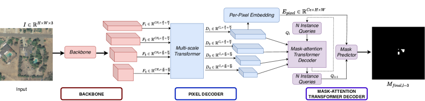
This section provides a detailed description of our transformer-based framework SolarFormer. This framework is specifically tailored for the segmentation of PV installations. As illustrated in Fig.2, our network comprises three distinct components: Network Backbone, Pixel Decoder, Mask-attention Transformer Decoder. Given an RGB image with dimensions , the network produces a corresponding segmentation mask of dimensions .
III-A Network Backbone
The first block of our architecture is represented by the Backbone networks, which extract features from the input image of dimensions to be further processed by the downstream architecture. Backbone networks are crucial in network design, and various implementations can be found in the literature. VGG [33], for instance, was developed as a deep CNN suitable for image classification, boasting a depth of up to 19 layers. However, its straightforward design, primarily consisting of pooling and fully connected layers, paved the way for other CNN backbones to rise to prominence. CNN backbones include ShuffleNet [34], Inception [35], DenseNet [36], EfficientNet [37], etc. One of the most popular backbone networks are Residual Networks (ResNets) [38]. This family of networks is based on blocks of convolution and pooling layers with skipped connections and recurrent units between them followed by batch normalization’s. The ResNet family has a variety of implementations: ResNet-50, ResNet-34, ResNet-101, etc. and has been widely used for image classification and semantic segmentation tasks. For our model, we will be using ResNet pretrained on ImageNet as the backbone for our implementation and testing the performance of two of its most popular varieties: ResNet-50 and ResNet-101.
By employing ResNet as our proposed model’s backbone, an input image is transformed into several multi-scale feature maps . In our model, we produce feature maps at multiple resolutions. Specifically, we generate four such feature maps denoted as , , and , where represents the number of channels, and is the size of the input image.
III-B Pixel Decoder
The Pixel Decoder module serves as an intermediary between the Backbone Network and the Mask-Attention Transformer Decoder. It consists of two main components: the Multi-Scale Transformer Encoder and the Per-Pixel Embedding Module. The first component produces enhanced embedding features whereas the later component generates per-pixel embeddings for the image, denoted as .
III-B1 Multi-Scale Transformer Encoder
This module takes the last four feature maps generated by the backbone network and processes them hierarchically. These feature maps are ordered from low to high resolution and flattened using an embedding projection to achieve a consistent channel size , obtaining where and is equal to the size of . The flattened embeddings are then merged into , where . Since the embedding features are flattened out of their original spatial shapes and scale level, they are supplemented with a learnable encodings and of shape . The three encodings are then passed through a Multi-Scale Transformer Encoder [39] to produce learned features from the input sequence, taking the embedded features and generating encoded features that capture the relationships between the elements. The correlated feature embeddings are then divided into groups based on the multi-scale level and restored to their original spatial shape with a fixed channel size as , , and .
III-B2 Per-Pixel Embedding Module
The second stage of the Pixel Decoder computes the pixel embeddings using the first feature layer outputted from the Multi-Scale Encoder. The goal of this process is to scale the to the original spatial shape of the image and creating . Each pixel in the represents both the semantic and mask classification of the corresponding pixel on the original image.
III-C Mask-attention Transformer Decoder
III-C1 Mask Predictor
To predict the segmented masks of possible instances in every image, per-pixel embeddings are utilised. The prediction process involves learning per-segment query embeddings , where represent the features of the maximun amount of possible instances in the image. Each then correlates with every pixel feature in and determines if the pixel belongs to the corresponding instance. Therefore, the predicted instance segmentation becomes .
III-C2 Mask-attention Transformer Decoder
This module decodes per-segment query embeddings from the encoded feature maps . The decoding procedure is done recurrently on different steps, where each step is associated to a layer from the encoded feature maps. At the first step we are processing the encoded feature layer with the lowest resolution , and we recurrently process each layer all the way to the highest resolution . At each of these layers, the query is decoded from the previous layer’s and its corresponding encoded feature maps.
A predicted mask is subsequently computed using the current query and the per-pixel embeddings and interpolated to the same size as . is then used as an attention mechanism that focuses on the salient parts of the features maps and allows for the query embeddings to attend to the features that are most important to the instances being decoded. Specifically, the attention mask is applied to during the decoding process to selectively attend to certain areas of the feature maps most relevant to the instance decoded.
III-C3 Segmentation Mask Prediction
The last step of the model generates the final segmentation masks . To do so, the query embeddings from the decoder at the last step , and the per-pixel embeddings are utilized to compute .
IV Experiments
IV-A Datasets
Our SolarFormer is benchmarked using three distinct RGB aerial imagery datasets. Each dataset is partitioned using a 60/20/20 split for training, testing, and validation, respectively. To maintain uniformity, the total number of images featuring PV installations is equally distributed across these divisions. The annotated data primarily consists of two classes: PV installation and background. The datasets sourced were from three distinct regions:
USGS, California: This aerial imagery, sourced from the United States Geological Survey (USGS), is part of their continued initiative to map various U.S. regions using detailed imagery, focusing specifically on California. Annotations are provided by [21]. This dataset boasts 601 TIF images, each with dimensions of 5000x5000 pixels and a resolution finer than 30 cm/pixel. Each image represents a 2.25 square kilometer area. For consistency across datasets, we extracted 400x400 patches from these images, resulting in a total of 37,660 images, of which 50.87% feature PV installations.
IGN, France: This large high-resolution aerial imagery dataset was gathered from the publicly available Institut géographique national (IGN) website in France. Similarly to the process followed with the California dataset, these images were annotated through a crowd-sourcing campaign [20]. The dataset contains 17,325 thumbnails sized 400-by-400 at a resolution of 20 cm/pixel with a share of 44.34 % containing solar installations.
GGE, France: While this dataset’s aerial imagery overlaps with the regions covered in the IGN, France dataset, the images were specifically derived from Google Earth Engine. Boasting a GSD of 10 cm/pixel, this resolution is the most refined of all datasets used in our experiments. The same crowd-sourcing initiative as mentioned in [20] was employed for annotations. This dataset includes 28,807 thumbnail images, each measuring 400x400 pixels, with a ratio of 46.11% depicting solar installations versus those that don’t.
| Methods | Solar PV Segmentation Performance on each dataset | ||||||||
|---|---|---|---|---|---|---|---|---|---|
| GGE, France | USGS, California | IGN, France | |||||||
| IoU | F1-score | Accuracy | IoU | F1-score | Accuracy | IoU | F1-score | Accuracy | |
| Zech et al., [18] | |||||||||
| 3D-PV-Locator [19] | 80.70 | 89.30 | 90.70 | 53.10 | 69.40 | 66.40 | |||
| Zhuang, et al., [17] | 84.39 | 91.60 | 90.89 | ||||||
| Our SolarFormer | 79.42 | 88.53 | 94.18 | 88.78 | 94.05 | 94.39 | 56.41 | 71.13 | 79.66 |
| Backbones | Networks | Solar PV Segmentation Performance on each dataset | ||||||||
|---|---|---|---|---|---|---|---|---|---|---|
| GGE, France | USGS, California | IGN, France | ||||||||
| IoU | F1-score | Accuracy | IoU | F1-score | Accuracy | IoU | F1-score | Accuracy | ||
| ResNet-50 | FCN [40] | |||||||||
| UNet [41] | ||||||||||
| PSPNet [42] | 77.79 | 87.50 | ||||||||
| UperNet [43] | 79.40 | 88.49 | ||||||||
| Mask2Former [44] | 90.73 | 85.33 | 92.08 | 92.80 | 87.63 | |||||
| Our SolarFormer | 93.08 | 87.39 | 93.27 | 92.76 | 56.06 | 71.84 | 82.25 | |||
| ResNet-101 | FCN [40] | |||||||||
| UNet [41] | ||||||||||
| PSPNet [42] | ||||||||||
| UperNet [43] | 79.19 | 88.40 | 52.20 | 68.59 | ||||||
| Mask2Former [44] | 92.39 | 86.98 | 93.03 | 94.10 | 66.52 | |||||
| Our SolarFormer | 79.42 | 88.53 | 94.18 | 88.78 | 94.05 | 94.39 | 56.41 | 71.13 | 79.66 | |
IV-B Evaluation Metrics
To assess the efficacy of our SolarFormer and compare it with existing methods, we utilize three standard metrics often employed in semantic segmentation evaluations: Intersection over Union (IoU), F1 score, and Accuracy. These metrics hinge on the comprehension and calculation of four key values: true positive (TP), true negative (TN), false positive (FP), and false negative (FN) as follows:
| (1) |
| (2) |
| (3) |
IV-C Implementation Details
IV-D Quantitative Results and Analysis
We evaluate our SolarFormer in terms of both network performance and network design efficiency. i. Network Performance: Our SolarFormer is compared with current state-of-the-art (SOTA) DL-based Solar PV profiling methods, as detailed in Table I. ii. Network Design Efficiency: We compare our SolarFormer against other prevalent DL-based segmentation models employing various backbone networks (i.e. ResnNet-50 and ResNet-101). This comparison is presented in Table II. These quantitative assessments were conducted across all three datasets.
i. Network Performance
Table I summarizes the performance of our SolarFormer against current SOTA methods for solar profiling. Our segmentation model outperforms Zech et al., [18], 3D-PV-Locator [19] and Zhuang, et al., [17] on all three datasets. For instance, when analyzing the USGS California dataset, our model exhibits substantial improvements, including an impressive 4.39% increase in IoU, a notable 2.45% enhancement in F1-score, and a substantial boost of 3.5% in Accuracy compared to the second-best method Zhuang, et al., [17]. Similarly, on IGN France, our model showcases remarkable advancements, with gains of 3.31%, 1.73%, and 13.26% in IoU, F1-score, and Accuracy, respectively, when compared to the runner-up method, 3D-PV-Locator [19].
ii. Network Design Efficiency Table II presents performance comparisons between our SolarFormer and the SOTA methods. Overall, our SolarFormer achieves its highest performance using ResNet-101, while the second-best performance is delivered by our SolarFormer implemented with ResNet-50.
GGE, France. Our SolarFormer demonstrates significant improvements over CNN-based models. Specifically, when benchmarked on the ResNet-101 backbone, it gains 0.23% IoU and 0.13% F1-score on UperNet [43] and improves the Accuracy result of Mask2former [44] by 1.79%. On the ResNet-50 backbone, SolarFormer outperforms the second best method, Mask2Former [44], by 2.35% on Accuracy. Although the high precision of the 10 cm/pixel GSD imagery likely aids SolarFormer in discerning finer image details, the granularity of the images prevents greater performance gains as shown on the other datasets.
USGS, California. Again, SolarFormer displays notable gains over both CNN-based models and the Mask2Former [44] on both ResNet backbones. For example on the ResNet-50 backbone, when compared to the top performing CNN-based model UperNet [43], SolarFormer gains 4.99% on IoU, 4.75% on F1-score and 3.19% on Accuracy. The difference with Mask2former [44] is still remarkable at 1.8%, 1.02% and 0.29%. Despite a high GSD, California’s vast aerial imagery and reduced granularity seem to enhance the model’s feature recognition.
IGN, France. Despite its lower resolution, SolarFormer exhibits robust scores against other models on the ResNet backbones. The dataset’s underwhelming performance is attributed to its lower resolution and limited imagery. Similar to GGE, France dataset, the granularity in the imagery might impact the model’s efficiency in detecting installations. For example, when benchmarked on the ResNet-101 backbone, it achieves gains of 4.21% on Iou and 2.54% on the UperNet [43] and 13.14% on Accuracy on the Mask2Former [44].
IV-E Qualitative Results and Analysis
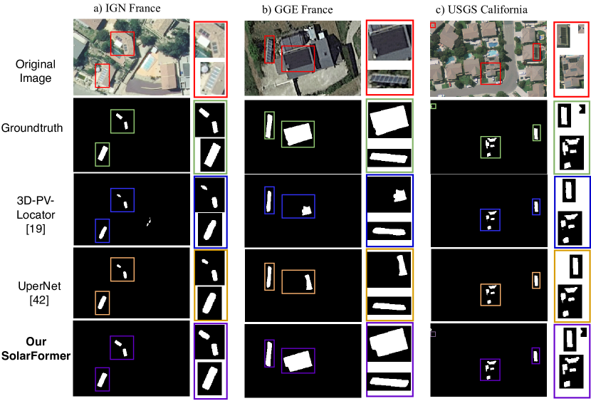
In this section, we provide a qualitative comparison of SolarFormer against widely-used baseline models: DeepLabV3+ [45] and UperNet [43]. We’ll highlight the advancements of our model in addressing challenges previously outlined.
Small objects: Fig. 3 a) and c) highlight SolarFormer’s proficiency in identifying small objects, even as diminutive as solar cells measuring pixels, underscoring its potential in high-resolution aerial imagery. Intra-class heterogeneity: Figs.3 a), b), c) illustrate the diverse PV installations even within a single rooftop. The variety in shapes, colors, and orientations poses challenges for deep learning. Notably, SolarFormer accurately maps varied color cells in Fig. 3 a) and identifies accurate boundary in Fig. 3 b).
Inter-class heterogeneity: Figs.3 b), c) depict challenges due to visual similarities between PV installations and other elements. In Fig. 3 b), while both DeepLabV3+ and UperNet falter due to the rooftop’s similar tone to PV installations, SolarFormer excels. In Fig. 3 c), DeepLabV3+ erroneously misidentifies a pool reflection as a solar cell.
Overall performance: Fig. 3 exhibits SolarFormer’s superior ability to accurately depict PV installations, outperforming baseline models in clarity and precision. It identifies minute panels throughout the image and consistently offers robust results with minimal background confusion.
V Conclusion
In this research, we introduced SolarFormer, an innovative Transformer-based model for solar PV profiling. Leveraging the Transformer architecture, SolarFormer adeptly learns high-resolution features and attend to the finer details while retaining complex relationships between them. This not only empowers SolarFormer with a comprehensive context but also lets it extract rich visual cues, as underscored by the robust results achieved. Thus, SolarFormer is able to address the solar PV challenges including low-resolution, inter-/intra-class homogenity.
We benchmarked SolarFormer against current SOTA Solar-PV profiling methods and evaluated its performance alongside various CNN-based and Transformer-based segmentation networks using both ResNet-50 and ResNet-101 backbones. Our comprehensive quantitative analysis confirms that SolarFormer surpasses the results of other prevalent segmentation networks. Furthermore, our qualitative findings underscore its enhancements over prior methodologies.
References
- [1] I. M. Peters, C. D. R. Gallegos, S. E. Sofia, and T. Buonassisi, “The value of efficiency in photovoltaics,” Joule, vol. 3, no. 11, pp. 2732–2747, 2019.
- [2] A. C. Lemay, S. Wagner, and B. P. Rand, “Current status and future potential of rooftop solar adoption in the united states,” Energy Policy, vol. 177, p. 113571, 2023.
- [3] “Record u.s. small-scale solar capacity was added in 2022,” https://www.eia.gov/todayinenergy/detail.php?id=603411.
- [4] M. Pierro, D. Gentili, F. R. Liolli, C. Cornaro, D. Moser, A. Betti, M. Moschella, E. Collino, D. Ronzio, and D. van Der Meer, “Progress in regional pv power forecasting: A sensitivity analysis on the italian case study,” Renewable Energy, vol. 189, pp. 983–996, 2022.
- [5] H. Shaker, H. Zareipour, and D. Wood, “A data-driven approach for estimating the power generation of invisible solar sites,” IEEE Transactions on Smart Grid, vol. 7, no. 5, pp. 2466–2476, 2015.
- [6] J. Yu, Z. Wang, A. Majumdar, and R. Rajagopal, “Deepsolar: A machine learning framework to efficiently construct a solar deployment database in the united states,” Joule, vol. 2, no. 12, pp. 2605–2617, 2018.
- [7] S. J. O’neill, M. Boykoff, S. Niemeyer, and S. A. Day, “On the use of imagery for climate change engagement,” Global environmental change, vol. 23, no. 2, pp. 413–421, 2013.
- [8] N. Said, K. Ahmad, M. Riegler, K. Pogorelov, L. Hassan, N. Ahmad, and N. Conci, “Natural disasters detection in social media and satellite imagery: a survey,” Multimedia Tools and Applications, vol. 78, pp. 31 267–31 302, 2019.
- [9] S. P. B, P. Sheladiya Kaushik, J. Patel, C. R. Patel, and R. M. Tailor, “Assessing land suitability for managing urban growth: An application of gis and rs,” in IGARSS 2020 - 2020 IEEE International Geoscience and Remote Sensing Symposium, 2020, pp. 4243–4246.
- [10] H. A. Effat and M. N. Hegazy, “A multidisciplinary approach to mapping potential urban development zones in sinai peninsula, egypt using remote sensing and gis,” J.of Geographic Information System, vol. 2013, 2013.
- [11] J. Wang, Z. Zheng, A. Ma, X. Lu, and Y. Zhong, “Loveda: A remote sensing land-cover dataset for domain adaptive semantic segmentation,” arXiv preprint arXiv:2110.08733, 2021.
- [12] G. Kasmi, L. Dubus, P. Blanc, and Y.-M. Saint-Drenan, “Towards unsupervised assessment with open-source data of the accuracy of deep learning-based distributed pv mapping,” in Workshop on Machine Learning for Earth Observation (MACLEAN), 2022.
- [13] P. Parhar, R. Sawasaki, A. Todeschini, H. Vahabi, N. Nusaputra, and F. Vergara, “Hyperionsolarnet: solar panel detection from aerial images,” arXiv preprint arXiv:2201.02107, 2022.
- [14] A. Vaswani, N. Shazeer, N. Parmar, J. Uszkoreit, L. Jones, A. N. Gomez, L. u. Kaiser, and I. Polosukhin, “Attention is all you need,” in Advances in Neural Information Processing Systems, I. Guyon, U. V. Luxburg, S. Bengio, H. Wallach, R. Fergus, S. Vishwanathan, and R. Garnett, Eds., vol. 30. Curran Associates, Inc., 2017.
- [15] J. M. Malof, K. Bradbury, L. M. Collins, and R. G. Newell, “Automatic detection of solar photovoltaic arrays in high resolution aerial imagery,” Applied energy, vol. 183, pp. 229–240, 2016.
- [16] J. M. Malof, L. M. Collins, and K. Bradbury, “A deep convolutional neural network, with pre-training, for solar photovoltaic array detection in aerial imagery,” in 2017 IEEE International Geoscience and Remote Sensing Symposium (IGARSS), 2017, pp. 874–877.
- [17] L. Zhuang, Z. Zhang, and L. Wang, “The automatic segmentation of residential solar panels based on satellite images: A cross learning driven u-net method,” Applied Soft Computing, vol. 92, p. 106283, 2020.
- [18] M. Zech and J. Ranalli, “Predicting pv areas in aerial images with deep learning,” in 2020 47th IEEE Photovoltaic Specialists Conference (PVSC), 2020, pp. 0767–0774.
- [19] K. Mayer, B. Rausch, M.-L. Arlt, G. Gust, Z. Wang, D. Neumann, and R. Rajagopal, “3d-pv-locator: Large-scale detection of rooftop-mounted photovoltaic systems in 3d,” Applied Energy, vol. 310, p. 118469, 2022.
- [20] G. Kasmi, Y.-M. Saint-Drenan, D. Trebosc, R. Jolivet, J. Leloux, B. Sarr, and L. Dubus, “A crowdsourced dataset of aerial images with annotated solar photovoltaic arrays and installation metadata,” Scientific Data, vol. 10, no. 1, p. 59, 2023.
- [21] K. Bradbury, R. Saboo, T. L Johnson, J. M. Malof, A. Devarajan, W. Zhang, L. M Collins, and R. G Newell, “Distributed solar photovoltaic array location and extent dataset for remote sensing object identification,” Scientific data, vol. 3, no. 1, pp. 1–9, 2016.
- [22] A. Dosovitskiy, L. Beyer et al., “An image is worth 16x16 words: Transformers for image recognition at scale,” in ICLR, 2021.
- [23] A. Gillioz, J. Casas, E. Mugellini, and O. A. Khaled, “Overview of the transformer-based models for nlp tasks,” in 15th Conference on Computer Science and Information Systems, 2020, pp. 179–183.
- [24] H. Touvron, M. Cord, M. Douze, F. Massa, A. Sablayrolles, and H. Jégou, “Training data-efficient image transformers & distillation through attention,” in International conference on machine learning. PMLR, 2021, pp. 10 347–10 357.
- [25] H. K. Joo, K. Vo, K. Yamazaki, and N. Le, “Clip-tsa: Clip-assisted temporal self-attention for weakly-supervised video anomaly detection,” in 2023 IEEE International Conference on Image Processing (ICIP). IEEE, 2023, pp. 3230–3234.
- [26] K. Yamazaki, S. Truong, K. Vo, M. Kidd, C. Rainwater, K. Luu, and N. Le, “Vlcap: Vision-language with contrastive learning for coherent video paragraph captioning,” in 2022 IEEE International Conference on Image Processing (ICIP). IEEE, 2022, pp. 3656–3661.
- [27] K. Yamazaki, K. Vo, Q. S. Truong, B. Raj, and N. Le, “Vltint: visual-linguistic transformer-in-transformer for coherent video paragraph captioning,” in Proceedings of the AAAI Conference on Artificial Intelligence, vol. 37, no. 3, 2023, pp. 3081–3090.
- [28] K. Vo, K. Yamazaki, P. X. Nguyen, P. Nguyen, K. Luu, and N. Le, “Contextual explainable video representation: Human perception-based understanding,” in 2022 56th Asilomar Conference on Signals, Systems, and Computers. IEEE, 2022, pp. 1326–1333.
- [29] K. Vo, S. Truong, K. Yamazaki, B. Raj, M.-T. Tran, and N. Le, “Aoe-net: Entities interactions modeling with adaptive attention mechanism for temporal action proposals generation,” International Journal of Computer Vision, vol. 131, no. 1, pp. 302–323, 2023.
- [30] P. Sun, R. Zhang, Y. Jiang, T. Kong, C. Xu, W. Zhan, M. Tomizuka, L. Li, Z. Yuan, C. Wang et al., “Sparse r-cnn: End-to-end object detection with learnable proposals,” in Proceedings of the IEEE/CVF conference on computer vision and pattern recognition, 2021, pp. 14 454–14 463.
- [31] M. Tran, K. Vo, K. Yamazaki, A. Fernandes, M. Kidd, and N. Le, “Aisformer: Amodal instance segmentation with transformer,” British Machine Vision Conference (BMVC), 2022.
- [32] T.-P. Nguyen, T.-T. Pham, T. Nguyen, H. Le, D. Nguyen, H. Lam, P. Nguyen, J. Fowler, M.-T. Tran, and N. Le, “Embryosformer: Deformable transformer and collaborative encoding-decoding for embryos stage development classification,” in The IEEE/CVF Winter Conference on Applications of Computer Vision, 2023, pp. 1981–1990.
- [33] K. Simonyan and A. Zisserman, “Very deep convolutional networks for large-scale image recognition,” arXiv preprint arXiv:1409.1556, 2014.
- [34] X. Zhang, X. Zhou, M. Lin, and J. Sun, “Shufflenet: An extremely efficient convolutional neural network for mobile devices,” in Proceedings of the IEEE conference on computer vision and pattern recognition, 2018, pp. 6848–6856.
- [35] C. Szegedy, W. Liu, Y. Jia, P. Sermanet, S. Reed, D. Anguelov, D. Erhan, V. Vanhoucke, and A. Rabinovich, “Going deeper with convolutions,” in Proceedings of the IEEE conference on computer vision and pattern recognition, 2015, pp. 1–9.
- [36] G. Huang, Z. Liu, L. Van Der Maaten, and K. Q. Weinberger, “Densely connected convolutional networks,” in Proceedings of the IEEE conference on computer vision and pattern recognition, 2017, pp. 4700–4708.
- [37] M. Tan and Q. Le, “Efficientnet: Rethinking model scaling for convolutional neural networks,” in International conference on machine learning. PMLR, 2019, pp. 6105–6114.
- [38] K. He, X. Zhang, S. Ren, and J. Sun, “Deep residual learning for image recognition,” in Proceedings of the IEEE conference on computer vision and pattern recognition, 2016, pp. 770–778.
- [39] A. Dosovitskiy, L. Beyer, A. Kolesnikov et al., “An image is worth 16x16 words: Transformers for image recognition at scale,” in International Conference on Learning Representations, 2021.
- [40] J. Long, E. Shelhamer, and T. Darrell, “Fully convolutional networks for semantic segmentation,” in Proceedings of the IEEE conference on computer vision and pattern recognition, 2015, pp. 3431–3440.
- [41] O. Ronneberger, P. Fischer, and T. Brox, “U-net: Convolutional networks for biomedical image segmentation,” in Medical Image Computing and Computer-Assisted Intervention–MICCAI. Springer, 2015, pp. 234–241.
- [42] H. Zhao, J. Shi, X. Qi, X. Wang, and J. Jia, “Pyramid scene parsing network,” in Proceedings of the IEEE conference on computer vision and pattern recognition, 2017, pp. 2881–2890.
- [43] T. Xiao, Y. Liu, B. Zhou, Y. Jiang, and J. Sun, “Unified perceptual parsing for scene understanding,” in Proceedings of the European conference on computer vision (ECCV), 2018, pp. 418–434.
- [44] B. Cheng, I. Misra, A. G. Schwing, A. Kirillov, and R. Girdhar, “Masked-attention mask transformer for universal image segmentation,” in Proceedings of the IEEE/CVF Conference on Computer Vision and Pattern Recognition (CVPR), June 2022, pp. 1290–1299.
- [45] L.-C. Chen, G. Papandreou, F. Schroff, and H. Adam, “Rethinking atrous convolution for semantic image segmentation,” arXiv preprint arXiv:1706.05587, 2017.
- [46] D. P. Kingma and J. Ba, “Adam: A method for stochastic optimization,” arXiv preprint arXiv:1412.6980, 2014.