On the data-driven description of lattice materials mechanics

Abstract

In the emerging field of mechanical metamaterials, using periodic lattice structures as a primary ingredient is relatively frequent. However, the choice of aperiodic lattices in these structures presents unique advantages regarding failure, e.g., buckling or fracture, because avoiding repeated patterns prevents global failures, with local failures occurring in turn that can beneficially delay structural collapse. Therefore, it is expedient to develop models for computing efficiently the effective mechanical properties in lattices from different general features while addressing the challenge of presenting topologies (or graphs) of different sizes. In this paper, we develop a deep learning model to predict energetically-equivalent mechanical properties of linear elastic lattices effectively. Considering the lattice as a graph and defining material and geometrical features on such, we show that Graph Neural Networks provide more accurate predictions than a dense, fully connected strategy, thanks to the geometrically induced bias through graph representation, closer to the underlying equilibrium laws from mechanics solved in the direct problem. Leveraging the efficient forward-evaluation of a vast number of lattices using this surrogate enables the inverse problem, i.e., to obtain a structure having prescribed specific behavior, which is ultimately suitable for multiscale structural optimization problems.

1 Introduction

1.1 Motivation

Lattice structures in the form of micro-architected lattices constitute a building block for the emerging field of mechanical metamaterials, which have gained attention recently due to their tuneable properties compared to their conventional bulk materials [1, 2, 3]. This versatility [4] in their properties makes them a perfect candidate for structural optimization problems, which poses an additional challenge given that metamaterials span several scales, i.e., yielding the subsequent multiscale problem [5, 6]. The application of lattice materials in engineering fields demands real-time calculations, which require the fast evaluation of models, e.g., the mentioned structural optimization [7] or structural health monitoring (SHM) [8].

In the framework of multiscale optimization problems, different techniques are used for computing the homogenized or equivalent behavior—see Somnic et al. for a more in-depth review on lattice materials [9]. To compute the effective behavior, e.g., stiffness, of lattice structures spanning different length scales, numerical techniques addressing the full-resolution of the structure, such as FE² [10] emerge to carry out this multiscale problem, but at a high computational cost. Homogenization methods [11] such as FFT homogenization [12, 13] overcome this expensive problem. However, this method presents issues when there are two phases with different stiffness, very pronounced in the case of lattice materials since one of the phases is void, i.e., null stiffness—the so-called infinite stiffness contrast in FFT homogenization methods [14].

Data-driven techniques bypass this expensive step, thus allowing for fast evaluations by building less complex surrogate or reduced order models [15] that learn the (potentially) complex underlying physical phenomena, e.g., using machine learning (ML) or deep learning (DL) algorithms. Once the surrogate models have been trained in an offline phase, they present benefits in different applications in the online phase, e.g., metamaterial characterization and optimization, boosting the computation speed for additional simulations within a multiscale optimization framework, or fast prediction in real-time scenarios, among others. These approaches are widely applied in other engineering fields, like solving complex numerical problems such as parameterized partial differential equations (PDEs) [16, 17, 18].

A popular technique in recent years is the so-called physics-informed neural network (PINN) [19, 20], directly imposing the physical equations in the problem, e.g., by introducing the corresponding residual in the loss function. PINNs ultimately allow for the solution of forward and inverse problems [21, 22]—noting the ill-posedness of the latter [23, 24]. Initially, the challenges tackled by DL use dense neural networks (DNNs), achieving a good level of precision [25]. However, they typically require many trainable parameters and a fixed, i.e., dense, input vector. Thus, other architectures such as graph neural networks (GNNs) [26], overcome this step by dealing with variable-size input data (graphs), succeeding to learn from simple essential mechanics such as linear elasticity up to more complex non-linear problems [27] with a much smaller number of parameters.

1.2 Related research

Most metamaterial lattices in the literature are periodic and symmetric—built by repetition of a parametric unit cell, which significantly eases their design and manufacturing. Nevertheless, that fact also makes them vulnerable to the propagation of mechanical issues such as buckling, fatigue, or creep. Having identical struts orderly distributed throughout space means that, should any of them reach critical conditions, the rest will contribute to transform a local failure into a global one.

A solution to that would be an aperiodic lattice so that no two struts would be identical, and thus, never share the exact critical requirements. Aperiodic lattices also present advantageous applications in fracture, e.g., toughness improvement [28], and vibration suppression, e.g., enhanced damping [29]. While aperiodic designs are being designed and tested [30, 31], a unified framework or methodology relating their architecture to their final properties remains elusive, let alone inverse analysis (obtaining a tailored architecture from the desired performance, although some promising ML-based techniques have been developed [32]).

In periodic metamaterials, the geometry and topology of the unit cell are tightly defined beforehand. However, more rigorous classifications have been proposed [33] and optimized [34]. Their properties can usually be obtained – at least, partially – from their geometry via experimental testing [35], the Finite Element Method (FEM) [36] and NNs [37]. This is different for (semi)randomly-generated architectures, so the first step would be to find a robust way to classify them, i.e. telling them apart from each other so their relative advantages and inconveniences can be evaluated.

Some statistical descriptors are already used for heterogeneous media like alloys or composites [38, 39]. Topological Data Analysis (TDA) [40, 41], despite being more widespread in scenarios where one wishes to make sense out of and/or correlate data cloud points to extract the underlying behavior law – such as contagion scenarios [42] – has been successfully used to classify composites [43]. Nonetheless, some studies suggest a topological perspective may not suffice to capture nor predict the metamaterial’s mechanical behavior [35] and call to incorporate homogenization [44], affinity deformation considerations between different phases (unit cells) [45] or even ML to capture nonlinear responses [46]. Homogenization is ever-important in lattices as a method for accurate, simplified behavior portrayal [47, 48, 49], either in a purely analytical form [50, 51] or in reverse [52], via FEM [53] or graph-assisted with varied applications [54, 55, 56, 57].

ML-based tools such as Convolutional Neural Networks (CNNs), Genetic Algorithms, or DL have been applied in metamaterial design [58] or fracture mechanism forecast [59]. In particular, GNNs [60] and Message-Passing [61] have proven very useful for capturing – and optimizing [62] – the topology while learning the underlying physics and the respective conservation laws. They have been used in surrogate modeling [63] and prediction of mechanical behavior such as buckling [64], fracture [65, 66], fatigue [67] and nonlinear stress/strain relationships [68], which are crucial needs in SHM.

GNNs can be further enriched by introducing the PDEs describing the physical phenomenon to be replicated in a similar fashion to the aforementioned PINNs [69, 70]—which can also be expanded by graph theory [71]. Some variants of this mixture have tackled unstructured meshes [21], natural convection in fluid dynamics [72], microneedle design [73], soft-tissue mechanics [74] or production forecasting [75].

All these tools can be viewed as surrogate models since they bypass the need for accurate analytical expressions to describe or predict the material’s behavior, mechanical in this case. Delving into non-deterministic problems, they pose an extra issue since the outcome is not known in advance, so models – such as neural networks – cannot be “trained” as easily. Although bibliography on the topic remains scarce, some non-deterministic/stochastic surrogate examples can be found [76, 77, 78], even for the prediction of material properties [79, 80]; namely fatigue [81], fracture [82] and corrosion [83].

1.3 Materials and methods

In this paper, we build a surrogate mechanical model to predict the equivalent, effective behavior of lattice materials, thus alleviating the computationally expensive associated cost compared to, e.g., an FE² approach [10]. To this end, we present and describe the offline phase of this process, showcasing some examples of applications with a synthetically generated dataset. We create our dataset with randomized, unit cell structures due to the highlighted properties that they pose.

We set a random number of nodes within a cubic domain and connect them through Delaunay triangulation [84, 85], using either pin-jointed trusses or Euler-Bernoulli beams to model the members/bars of the structures. This way, the lattice structures generated present different numbers of nodes and struts, which poses a challenge for architectures presenting a fixed number of inputs, e.g., regular DNNs. All the structures are labeled with their mechanical equivalent properties, namely Young’s moduli $E_{z}^{\rm eq}$ in $z-$axis, computed using an energy-preserving method as the relationship between the reaction forces and a prescribed displacement.

The effective behavior is computed by fitting an ML surrogate mechanical model, similar to other research conducted on this topic [86], adding the challenge of developing a model able to deal with lattices/meshes of different sizes and resolutions. Regarding the surrogate model, we propose two non-intrusive, NN architectures to predict the so-mentioned equivalent mechanical property: (1) a DNN approach fed with ‘engineered’ features, and (2) a GNN model using the geometry and material of the structure as inputs.

We first explore the use of a DNN aimed at predicting the mechanical properties with the minimum physical information, e.g., not providing the assembled stiffness matrix but rather the geometry or material properties of the lattice struts. In order to deal with samples presenting different (input) dimensions – number of nodes, number of members – reduced techniques shall be applied, e.g., projecting, averaging, interpolating, or pooling. One option is the proper orthogonal decomposition with artificial NN, i.e., POD-ANN [87], which consists of projecting the input space in a lower dimension manifold $\mathcal{M}\subset\mathbb{R}^{d}$, where $d$ is fixed so the latent space of all structures can be fed in the same dense architecture. This can be achieved using linear, e.g., PCA [88], or nonlinear, e.g., autoencoder techniques—similar to [27].

This approach becomes a challenging task, leading to the loss of crucial information in the encoding, such as the connectivity of the members within the lattice. Therefore, the DNN approach addressed in this paper is different. A structure is sliced into a certain number of slices in its three directions. In each slice, the sum of effective areas of intersected bars is computed. The total effective area per slice is fed to a DNN model with $3n_{s}$ inputs, where $n_{s}$ is the number of slices selected. Thus, we elaborate a physical analogy with a structure with multiple one-dimensional springs stacked in series. Each slice would represent springs in parallel—hence the sum. An illustrative example of this analogy is described in Section 3.1.

This way, we provide the maximum physical knowledge without directly feeding the (assembled) stiffness matrix of the structure. However, the previous perspective lacks topological information on the structures, hence the exploration of architectures accounting for the connectivity of the nodes as the training model, like GNN. With a graph-level regression GNN, we show an even higher level of accuracy using only as input the coordinates of the nodes, the connectivity, and properties of the members. We note that whereas DNNs explain better what it means to learn the material, GNNs succeed in learning the structure. Taking all the previous into account, we derive a model for computing effective properties, improving the commonly used models that are based on empirical exponential laws relating the stiffness to strut radius, i.e., the relative density of the cell [35]. In fact, due to the non-bijectivity of the model, the density can be considered an extra degree of freedom.

Once surrogate models of sufficient quality are obtained, the inverse analysis might be performed by efficiently (forward-)evaluating a large number of samples. Furthermore, the non-bijectivity of the problem allows for multiple lattices behaving similarly, thus leaving room to optimize a second variable, such as the weight of the structure, in the subsequent multi-objective optimization problem that might be addressed making use of Pareto optimality [89]. This addresses the issue of multiscale optimization proposed in [90], with the advantage of replacing the macro-to-micro step dependent on empirical laws in the latter with the forward-evaluation of the derived surrogate models proposed in this paper.

2 Lattice structures database

2.1 Structure definition

Each lattice structure is defined in a unit cube $\Omega\subset\mathbb{R}^{3}$ and its made of $n_{j}$ nodes (or joints) and $n_{e}$ members (or struts). Eight nodes of the lattice correspond to the vertex of the cube, thus they have a fixed position, whereas the remaining $n_{j}-8$ user-prescribed joints are randomly distributed within the domain $\Omega$. In this paper, samples are generated varying this number from 1 to 50. The 8 fixed nodes act as clamps in which forces or displacements will be applied, being the only nodes whose coordinates are fixed for all experiments so their results can be compared. The rest of the nodes’ coordinates are sampled from three independent and identically distributed (iid) random distributions $\mathcal{U}\left(\epsilon,1-\epsilon\right)$, where $\epsilon$ is a small value to prevent the randomly located joints from being on the boundary $\partial\Omega$ of the domain.

The elements are defined by a 3D generalization of Delaunay’s triangulation (through Bowyer-Watson’s algorithm [84, 85]), yielding a total $n_{e}$ elements, hence this number is not prescribed. Delaunay’s method, common in simulation software like ANSYS©, ensures both the absence of unforeseen – and undesired – intersections (nodes) and the strut lengths being constrained to a given interval despite their variability. In mechanical terms, it also reduces buckling (struts’ slenderness is contained within the aforementioned interval) and prevents the generation of sliver triangles presenting acute angles which would cause stress concentration and instabilities - mechanisms - if the truss is pin-jointed.

2.2 Boundary conditions

A lattice is subjected to a uniaxial test with an imposed displacement $u^{*}$ along the vertical direction ($z-$axis), as it is shown in Figure 1. Due to the three symmetry planes, some degrees of freedom are restricted (or fixed).

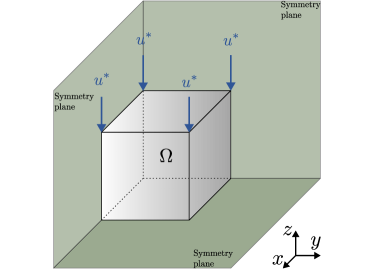
(a) Imposed displacement and symmetry planes

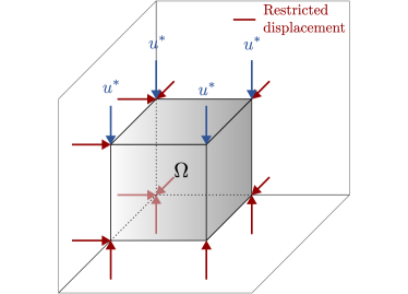
(b) Resulting boundary conditions

Figure 1: Boundary conditions of the lattice structure, where $u^{*}$ is the imposed displacement, in blue. The symmetry planes represented in green in (a) imply the restricted displacements in (b), depicted in red.

In the following, the free degrees of freedom are denoted by $f$, and the restricted ones by $r$. The latter comprise both the imposed and fixed displacements—blue and red arrows in Figure 1, respectively.

2.3 Mechanical model of the lattice

The elements of the lattice are modelled either as a pin-jointed truss structure, an Euler-Bernoulli beam, or a Timoshenko beam. The (linear) equilibrium equation for a lattice structure with $n_{d}$ degrees of freedom – equal to $3n_{j}$ for trusses, and $6n_{j}$ for beams – reads

$$\bm{K}\bm{u}=\bm{f},$$ (1)

where $\bm{u}\in\mathbb{R}^{n_{d}}$ and $\bm{f}\in\mathbb{R}^{n_{d}}$ are respectively the global stiffness matrix, the nodal displacements and the nodal forces vector, and $\bm{K}\in\mathbb{R}^{n_{d}\times n_{d}}$ is the global stiffness matrix of the whole structure without having imposed the boundary conditions. The local stiffness matrix of a truss is defined as

$$\bm{K}_{e}=\dfrac{E_{e}A_{e}}{l_{e}}\begin{bmatrix}1&0&0&-1&0&0\\ 0&0&0&0&0&0\\ 0&0&0&0&0&0\\ -1&0&0&1&0&0\\ 0&0&0&0&0&0\\ 0&0&0&0&0&0\\ \end{bmatrix},$$ (2)

where $E_{e}$, $A_{e}$ and $l_{e}$ are the stiffness, cross-sectional area and length of member $e$; whereas the 12 degrees-of-freedom Euler-Bernoulli or Timoshenko beam local stiffness matrices can be found in Equation (5.116) of [91]. Note that the global stiffness matrix used in this work comes from the direct stiffness method (DSM), but it can be extended to other forms of deriving the stiffness matrix, e.g. with FE discretization.

The equilibrium equation in (1) can be split by means of free $f$ and restricted $r$ degrees of freedom as

$$\left[\BMAT[2pt,0pt,1.5cm]{c;c}{c;c}\bm{K}_{ff}&\bm{K}_{fr}\\ \bm{K}_{rf}\bm{K}_{rr}\right]\left[\BMAT[2pt,0pt,1.5cm]{c}{c;c}\bm{u}_{f}\\ \bm{u}_{r}\right]=\left[\BMAT[2pt,0pt,1.5cm]{c}{c;c}\bm{0}\\ \bm{f}_{r}\right],$$ (3)

where the nodal forces vector in the free degrees of freedoms has been set to $\bm{f}_{f}=\bm{0}$ since the loading is purely displacements imposition. Performing a static condensation, the vector of nodal displacements of the free degrees of freedom $\bm{u}_{f}$ is

$$\bm{u}_{f}=-\bm{K}_{ff}^{-1}\bm{K}_{fr}\bm{u}_{r},$$ (4)

and the nodal forces on the restricted nodes (reactions) are

$$\bm{f}_{r}=\left(\bm{K}_{rr}-\bm{K}_{rf}\bm{K}_{ff}^{-1}\bm{K}_{fr}\right)\bm{u}_{r}.$$ (5)

With that, we compute the work of external forces $\mathcal{W}_{\rm ext}$ of the lattice

$$\mathcal{W}_{\rm ext}=\bm{f}\cdot\bm{u}=\bm{f}_{r}\cdot\bm{u}_{r}.$$ (6)

2.4 Effective behavior

We define an effective material of volume $|\Omega|$ energetically equivalent to the lattice structure. Then, we perform a uniaxial test and equate the energies to compute the equivalent stiffness of the lattice, specifically the Young’s modulus along $z-$axis direction—see Figure 1. The potential of the internal forces of the equivalent solid $\Pi_{\rm int}^{\rm eq}$ is

$$\Pi_{\rm int}^{\rm eq}=\int_{\Omega}\bm{\sigma}^{\rm eq}\left(\bm{\varepsilon}^{\rm eq}(\bm{x})\right):\bm{\varepsilon}^{\rm eq}(\bm{x})\mathrm{d}V,$$ (7)

where $\bm{\sigma}^{\rm eq}$ and $\bm{\varepsilon}^{\rm eq}$ are the Cauchy stress and infinitesimal strain second-order tensors of the equivalent body, related through the (linear) constitutive law $\bm{\sigma}^{\rm eq}=\mathbb{C}^{\rm eq}:\bm{\varepsilon}^{\rm eq}$, being $\mathbb{C}$ the fourth-order stiffness tensor. Note that any stress-strain work conjugate might be used since the material is working under its linear regime. Particularizing the constitutive law for a uniaxial test yields $\sigma_{zz}^{H}=E_{z}^{\rm eq}\varepsilon_{zz}^{\rm eq}$, hence the integral in previous Equation (7) is straightforward to compute, namely

$$\Pi_{\rm int}^{\rm eq}=\sigma_{zz}^{\rm eq}\varepsilon_{zz}^{\rm eq}|\Omega|.$$ (8)

The imposed displacement $u^{*}$ is the same for both solids, therefore the (continuum-)equivalent strain $\varepsilon_{zz}^{\rm eq}$ is

$$\varepsilon_{zz}^{\rm eq}=\dfrac{u^{*}}{L_{z}},$$ (9)

where $L_{z}$ is the longitudinal dimension of the studied direction $z$, i.e., the vertical size of the structure. By energy balance, the potential of external forces and the potential of internal forces are equal, in both lattice and equivalent solids i.e., $\mathcal{W}_{\rm ext}=\Pi_{\rm int}^{\rm eq}$, yielding

$$\bm{f}_{r}\cdot\bm{u}_{r}=E_{z}^{\rm eq}\left(\dfrac{u^{*}}{L_{z}}\right)^{2}|\Omega|.$$ (10)

Taking into account that $|\Omega|=A_{z}L_{z}$ where $A_{z}$ is the cross-sectional area of the equivalent solid perpendicular to the studied direction, the equivalent stiffness in $z-$direction $E_{z}^{\rm eq}$ is obtained

$$E_{z}^{\rm eq}=\dfrac{\bm{f}_{r}\cdot\bm{u}_{r}}{u^{*}A_{z}}\dfrac{L_{z}}{u^{*}}.$$ (11)

Note that this is equivalent to compute the ratio of resultant of the reaction forces $\bm{f}_{r}$ at the top face and the cross-sectional area perpendicular to the loading application $A_{z}$, i.e. the equivalent stress $\sigma_{zz}$, and dividing it by the imposed strain $\varepsilon_{zz}$.

3 Dense Neural Networks model

We now turn to the DL prediction of the equivalent stiffness $E_{z}^{\rm eq}$, object of study of this paper. By making use of a toy example of linear springs arranged in series, we train the simplest DNN model with the most meaningful variables. Taking this example into account, we propose a procedure based on slicing and weighing a given pin-jointed truss lattice structure in order to predict the mentioned mechanical property by training another DNN model.

3.1 Prediction of springs arranged in series: a toy example

We consider the following 1D linear, elastic problem comprised of $n_{s}$ uniaxial elements with different axial stiffness $(EA)_{e}$ and equal length $\ell$ arranged in series, as depicted in Figure 2.

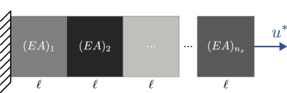
Figure 2: 1D linear, elastic problem comprised of $n_{s}$ elements of same length $\ell$ and different axial stiffness $(EA)_{e}$ arranged in series.

By elemental mechanics, the equivalent stiffness $K_{\rm eq}$ of $n_{s}$ springs arranged in series is given by

$$K_{\rm eq}^{-1}=\sum_{e=1}^{n_{s}}K_{e}^{-1}.$$ (12)

Considering the relation $K=EA/\ell$ between mechanical springs with constant $K$ and uniaxial elements (i.e., bar or truss) with axial stiffness $(EA)$ and length $\ell$ – which is also known from the theory of pin-jointed truss lattices – the equivalent stiffness of the system in Figure 2 is

$$(EA)_{\rm eq}=\dfrac{n_{s}}{\sum_{e}(EA)_{e}^{-1}}.$$ (13)

Therefore, this is the formula that the model would have to learn in case of approaching this problem with a DNN model. By means of the universal approximation theorem [92], this formula may be accurately represented by a sufficiently wide DNN architecture when given the stiffnesses of the members $(EA)_{e}$ as inputs. Thus, a DNN model is trained to prove the previous statement. The input features of this model are the inverse stiffness $1/(EA)_{e}$ of the elements since this allows the DNN to better approximate the target to predict $(EA)_{\rm eq}$ i.e., the function in Equation (13). The architecture used is described in Table 1. In the following, we consider $n_{s}=19$.

Layer	Neurons	Activation
Input layer	$n_{s}=19$	selu [93]
Hidden layer #1	$5n_{s}=95$	selu [93]
Output layer	$1$	linear

Table 1: Toy example. Hyper-parameters of the fully-connected DNN architecture.

Similarly, the training (hyper-)parameters are displayed in Table 2.

Parameter	Choice
Optimizer	nadam [94]
Learning rate	$0.001$
Epochs	2000
Loss, $\mathcal{L}$	MSE
Validation split	15%

Table 2: Toy example. (Hyper-)parameters of the training.

Furthermore, a learning rate reduction on plateau by $0.5$ is applied, as well as an early stopping criterion, both on the loss function. Lastly, the dataset is generated by drawing $N=20\,000\times n_{s}$ samples from a distribution $p(EA)\sim\mathcal{U}((EA)_{\min},(EA)_{\max})$, where $(EA)_{\min}=10$ and $(EA)_{\max}=100$. This way, a set of $\{\{(EA)_{e}^{(i)}\}_{e=1}^{n_{s}},(EA)_{\rm eq}^{(i)}\}_{i=1}^{N}$ is generated. A random train-test split of 15% is then applied, and both the features and targets are normalized with a standard scaler.

Once the training is performed, both the train and test metrics are computed. The DNN yields a loss of $\mathcal{L}_{\rm train}=\mathcal{L}_{\rm test}=1.32\cdot 10^{-3}$, and the coefficient of determination of $R^{2}_{\rm train}=0.9994$ and $R^{2}_{\rm test}=0.9993$. Denoting the prediction with a hat $\hat{\cdot}$, the train and test predictions are shown in a scatter plot in Figure 3, where the perfect prediction is given by the line at $45^{\circ}$.

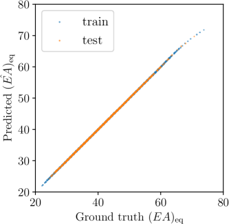
Figure 3: Toy example. Equivalent stiffness $E_{\rm eq}$ prediction, representing train and test in blue and orange, respectively. Although there is a slight under-prediction close to the upper limit, the precision is virtually perfect, with coefficients of determination $R^{2}_{\rm train}=0.9994$ and $R^{2}_{\rm test}=0.9993$.

Of course, this is a simple problem solved with an explicit formula, which is virtually perfectly approximated with a DNN model. We use the learnings from this method to address the effective behavior with a similar surrogate DNN model.

3.2 Slice features of the lattice structure

Analogously to the simple idea of the previous toy example, the (random) lattice structure of a given material is now sliced into $n_{s}$ parts. We formulate the following hypothesis: by defining an effective area per slice ($n_{s}$ in total), the prediction can be performed through an analogous approach to the toy example i.e., a DNN whose inputs are the inverse values of the effective areas. A schematic drawing of a general slice $s$ is depicted in Figure 4.

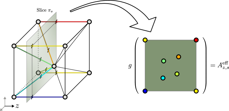
Figure 4: Scheme drawing of the lattice slicing perpendicular to $z-$axis for an arbitrary slice plane $\pi_{s}$. The joints are represented in gray, and the intersected bars are represented using a jet colormap. The effective area $A_{z,s}^{\rm eff}$ of the slice $s$ transverse to $z$ is computed by applying a function $g$ yet to be defined.

To define the effective area per slice, we introduce the function $g(\cdot)$, which is applied to the areas and directions of the intersected bars by the slice. Given an element $e$ with cross-sectional area $A_{e}$, and defined with its unit vector by $\bm{n}_{e}=[\cos\theta_{x,e},\cos\theta_{y,e},\cos\theta_{z,e}]^{\intercal}$, the effective area $A_{z,s}^{\rm eff}$ of the slice $s$ perpendicular to $z$ direction is computed as the sum of the projected areas along $z$ of the intersected bars in the plane $\pi_{s}$ i.e.,

$$A_{z,s}^{\rm eff}=\sum_{e\in\pi_{s}}A_{e}\cos^{2}\theta_{z,e}.$$ (14)

The quadratic exponent in the cosine function in Equation (14) comes from the projection of both the forces and displacements onto the local axis of the bar. An illustration of this is depicted in Figure 5. By simple rotations, the equivalent stiffness $K_{xx}^{\rm eq}$ in $x$ direction is obtained as the actual stiffness of the bar i.e., $EA/\ell$, multiplied by the cosine square of the angle between the bar and $x-$axis, namely

$$K_{xx}^{\rm eq}=\frac{EA}{\ell}\cos^{2}\theta_{x}.$$

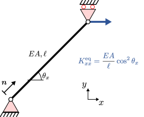
Figure 5: Equivalent stiffness $K_{xx}^{\rm eq}$ along direction $x$ in an example strut to show the quadratic exponent in the cosine function for computing the effective area. The bar is made of a material with Young’s modulus $E$, has cross-sectional area $A$ and length $\ell$, and presents an arbitrary inclination with respect to $x$ defined by the angle $\theta_{x}$.

The same definition applies to any other direction $d$, setting as input the corresponding cosine of the angle $\cos\theta_{d}$. Lastly, the transverse effective areas have to be considered when generalizing the problem from 1D to 2D or 3D.

Let I and II be two 2D lattice structures, with slightly different (square) unit cells of length $\ell$, depicted in Figure 6. All bars are of the same material with Young’s modulus $E$ and same cross-sectional area $A$. Both lattices I and II have the same effective area perpendicular to $x$ i.e., $A_{x,s}^{\rm eff}=3A$ for every slice $s$ contained in the structure, according to Equation (14). However, the equivalent stiffnesses $K_{xx}^{\rm eq}$ following the procedure derived in Section 2.4, are different in cases I and II i.e., $(K_{xx}^{\rm eq})_{\rm I}\neq(K_{xx}^{\rm eq})_{\rm II}$, due to transverse effects—lattice II is the same as lattice I with a (transverse) bar removed. Therefore, the effective areas $A_{y,s}^{\rm eff}$ perpendicular to $y$ have to be considered likewise in the surrogate model to make effective predictions for the general, non-1D case. Note that these effective areas for the lattices in Figure 6 are $(A_{y,s}^{\rm eff})_{\rm I}=2A$ and $(A_{y,s}^{\rm eff})_{\rm II}=A$.

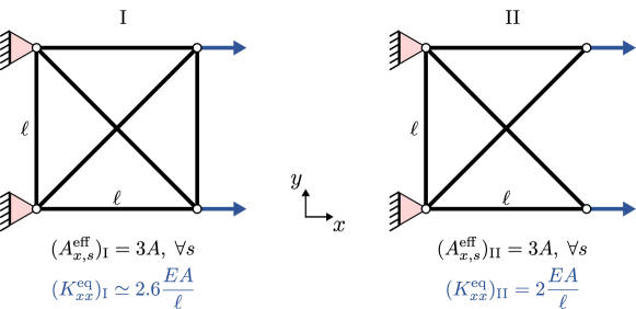
Figure 6: 2D lattice structures I and II made of different (square) unit cells of length $\ell$. Whereas the effective area transverse to $x$ is the same, $(A_{x,s}^{\rm eff})_{\rm I}=(A_{x,s}^{\rm eff})_{\rm II}=3A$ (for every slice $s$), the equivalent stiffness differs, $(K_{xx}^{\rm eq})_{\rm I}\simeq 2.6EA/\ell$ and $(K_{xx}^{\rm eq})_{\rm II}=2EA/\ell$. All bars are of the same material with Young’s modulus $E$ and same cross-sectional area $A$.

3.3 Results

Using the inverse of the effective transverse areas in the three spatial directions $A_{x,s}^{\rm eff}$, $A_{y,s}^{\rm eff}$, and $A_{z,s}^{\rm eff}$ for $n_{s}$ slices as inputs, a DNN model for 3D pin-jointed truss lattices is generated analogously to the toy example case shown in Section 3.1. The dataset is comprised of $10\,000$ randomly-generated samples i.e., lattices. The base material is AISI Type 316L Stainless Steel, annealed bar, with a Young’s modulus of $E_{\rm base}=193\,$GPa, and the lattice members are circular bars with radius $r=5\,$mm, leading to a cross-sectional area of $A=78.54\,$mm².

In order to select a suitable number $n_{s}$ of slices, the following limit analysis is performed on this number: the equivalent stiffness $(EA)_{z,\rm eq}$ of the lattices of the dataset is computed via Equation (13), using the effective area transverse to $z$ per slice $s$, $A_{z,s}^{\rm eff}$. Recall that we do not state that this is the actual equivalent stiffness to predict, but serves as a global value to make comparisons for this limit analysis. Then, these samples are sliced using different numbers of slices $n_{s}$.

The histogram of the equivalent stiffness $(EA)_{z,\rm eq}$ for the different $n_{s}$ used is depicted in Figure 7. Note that from $n_{s}=19$ on, this global magnitude per lattice is similarly distributed. Therefore, the number of slices used to feed the DNN model is set to $n_{s}=19$.

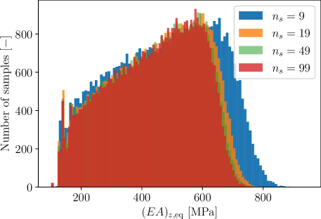
Figure 7: Pin-jointed truss lattice DNN model. Distribution of the equivalent stiffness $(EA)_{z,\rm eq}$ according to Equation (13) for different number of slices $n_{s}=\{9,19,49,99\}$.

Lastly, the equivalent stiffness to predict, $E_{z}^{\rm eq}$ – Equation (11) – is divided by the volume of the lattice to facilitate the predictions of the model. Namely, for each sample

$$\overline{E_{z}^{\rm eq}}=\dfrac{E_{z}^{\rm eq}}{V},$$ (15)

where $V$ is the volume of the lattice i.e.,

$$V=\sum_{e}A_{e}\ell_{e},$$ (16)

leading to the following dataset

$$\left\{\{(A_{x,s}^{\rm eff})^{(i)},(A_{y,s}^{\rm eff})^{(i)},(A_{z,s}^{\rm eff})^{(i)}\}_{s=1}^{n_{s}},\overline{E_{z}^{\rm eq}}^{(i)}\right\}_{i=1}^{N}.$$

The same architecture and optimization parameters displayed in Tables 1 and 2 are used. A validation set of 15% of the samples is separated, applying a train/test 85-15% split in the remaining dataset. Both the features and targets are normalized with a standard scaler. Once the training is performed, both the train and test metrics are computed. The DNN yields losses of $\mathcal{L}_{\rm train}=2.95\cdot{10}^{-2}$ and $\mathcal{L}_{\rm test}=3.58\cdot 10^{-2}$, and a coefficient of determination of $R^{2}_{\rm train}=0.971$ and $R^{2}_{\rm test}=0.965$. The predictions are depicted in a scatter plot in Figure 8.

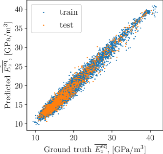
Figure 8: Pin-jointed truss lattice DNN model. Equivalent stiffness per unit volume $\overline{E_{z}^{\rm eq}}$ prediction, where the train and test are represented by blue and orange points, respectively

Although the solution is (obviously) less precise than the toy example, a certain level of accuracy is reached. Thus, a surrogate model via a non FE-based approach is developed. By just scanning in three directions a given lattice to compute its effective areas, and weighing the specimen to obtain its volume, the equivalent Young’s modulus can be effectively predicted.

4 Graph Neural Networks model

Now we interpret the lattice as a graph $\mathcal{G}(\mathcal{V},\mathcal{E})$, where the joints are the nodes $\mathcal{V}$ (also referred to as vertices), and the struts are the edges $\mathcal{E}$. Features can be defined for both the nodes and the edges, and so the GNN model is built. This architecture is agnostic to the input data size, only requiring a graph and its associated features. As an illustration, a properly trained graph-level task GNN is able to make predictions for two lattices with different topologies i.e., regardless of the differences in the number of joints and/or struts.

4.1 Features and architecture

In contrast to the DNN model, we will only provide the GNN geometrical features without physics or mechanics context, to assess whether the GNN is able to mimic the underlying equations, that is, equilibrium laws and computation of equivalent property. We define as node features the (three) spatial coordinates $(x_{j},y_{j},z_{j})$ of the joint $j$, whereas the edge features are the coordinates of both endpoints i.e., $(x_{e0},y_{e0},z_{e0}),(x_{e1},y_{e1},z_{e1})$ – where 0,1 represent both endpoints – and the associated length $\ell_{e}$ of the bar/beam $e$ represented by such edge. This leads to a total of seven edge features.

This way, we are providing structured, geometrical graph information to feed the GNN model. Since the base material used is the same (316 Stainless Steel), no material information is provided. Otherwise, it could be defined as a feature at the edge level. Additionally, the variable to be predicted is the equivalent Young’s modulus $E_{z}^{\rm eq}$ along $z-$axis. The dataset can be compactly represented as follows:

$$\left\{\{(x_{j}^{(i)},y_{j}^{(i)},z_{j}^{(i)})\}_{j=1}^{n_{j}},\{(x_{e0}^{(i)},y_{e0}^{(i)},z_{e0}^{(i)}),(x_{e1}^{(i)},y_{e1}^{(i)},z_{e1}^{(i)}),\ell_{e}^{(i)}\}_{e=1}^{n_{e}},{E_{z}^{\rm eq}}^{(i)}\right\}_{i=1}^{N}.$$

The architecture of the model comprises the following steps: (1) initial dense or fully connected (FC) layers applied separately for each node and edge, leading to subsequent node and edge embeddings, (2) two graph updates (or hops), updating the node embeddings, and (3) output layer based on pooling and FC layer. The details of these modules are displayed in Table 3.

Module	Layer	Input shape	Output shape	Activation
Node embedding	Dense	$(3,)$	$(5,)$	PReLU
Edge embedding	Dense	$(7,)$	$(5,)$	PReLU
	Message passing	$(15,)$	$(10,)$	selu
Graph Update #1	Convolution (mean)	$(10\times n_{m},)$	$(10,)$	$-$
	Dense	$(15,)$	$(10,)$	selu
	Message passing	$(25,)$	$(10,)$	selu
Graph Update #2	Convolution (mean)	$(10\times n_{m},)$	$(10,)$	$-$
	Dense	$(20,)$	$(10,)$	selu
	Pooling (mean)	$(10\times n_{j},)$	$(10,)$	$-$
Output	Dense	$(10,)$	$(1,)$	linear

Table 3: Pin-jointed truss lattice GNN model. Architecture of the graph-level task regression, where the second component of the shapes is the batch size which the model is fed with. Note that $n_{m}$ in the convolution layer stands for the number of messages (adjacencies) arriving to one node in the graph – different for each node – and $n_{j}$ in the pooling layer is the number of joints (nodes) per graph—different for every graph.

This architecture is sketched in Figure 9. Dense layers (depicted in yellow in the figure) are initially applied to each node and edge in the graph, outputting node and edge embeddings of size 5.

There are 2 graph updates (depicted in gray) which work as follows. (1) message passing: each edge computes a message by applying a dense layer to the concatenation of node states of both endpoints and the edge’s own feature embedding, leading to an input shape of 15, and selecting 10 units as the output of the message passing. (2) convolution: messages are averaged (permutation-invariant pooling) at the common nodes of edges. (3) dense: at each node, a dense layer is applied to the concatenation of the old node state with the averaged edge inputs (15 in total) to compute the new node state, which is defined by 10 features. This idea is illustrated in the figure in one arbitrary node of graph updates #1 and #2 using blue and purple arrows, respectively. Then, the pooling layer (blue) averages the node features – 10, given by the previous layer – across all the nodes in a graph i.e., the whole graph is now encoded into 10 features. Lastly, a dense layer (green) is applied to get the unique output (brown) i.e., the equivalent mechanical property to predict.

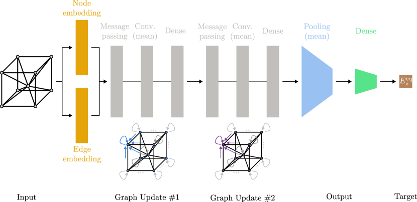
Figure 9: Pin-jointed truss lattice GNN model. Scheme drawing of the graph model’s architecture. The input is a lattice i.e., graph, and the goal is to predict an equivalent mechanical property of the lattice, namely the effective stiffness $E_{z}^{\rm eq}$ alongside $z-$axis. Initially, dense layers (depicted in yellow) are applied to every node and edge, leading to the subsequent node and edge embeddings. Then, the node features (or embeddings) are updated with 2 graph updates (depicted in gray). This update consists in a message passing where each edge computes a message by applying a dense layer to the concatenation of node states of both endpoints and the edge’s own feature embedding; a convolution averaging at the common nodes of edges, and a dense layer to compute the new node state. This idea is illustrated in one arbitrary node of graph updates #1 and #2 using blue and purple arrows, respectively. Lastly, a pooling layer (blue) averaging the features of all nodes is applied, followed by a dense layer (green) to compute the output to predict (brown).

4.2 Results for pin-jointed truss latices

We first assess the performance of the model in pin-jointed truss lattices. The design of experiments (DoE) is performed similarly by generating lattices using the same material (316L Stainless Steel) and strut geometry (circular strut with radius $r$). A dataset of $20\,000$ samples is created, and a 15% of them is taken as validation set i.e., $3000$ samples. Once the model is trained, other $2000$ samples are generated separately as a ‘hidden’ test set, representing another 10% of the combination of training and validation sets.

We recall that the structures within the dataset have different number of nodes – from 9 to 58, being fixed the 8 corner nodes – and hence with a varied number of elements, not necessarily the same for each sample. All the variables are scaled with standard normalization using the mean and standard deviation values of the training set. The optimization parameters are displayed in Table 4.

Parameter	Choice
Optimizer	nadam
Learning rate	$0.01$
Epochs	10 000
Loss, $\mathcal{L}$	MSE

Table 4: Pin-jointed truss lattice GNN model. Optimization parameters of the training.

The training yields $\mathcal{L}_{\rm train}=1.02\cdot 10^{-2}$ and $\mathcal{L}_{\rm test}=1.23\cdot 10^{-2}$, with coefficients of determination $R^{2}_{\rm train}=0.9900$ and $R^{2}_{\rm test}=0.9873$. The results of the prediction are depicted in Figure 10a. Note the more accurate prediction in the test set than in the previous model, being this a sign that the GNN outperforms the DNN model.

Being all the tests subjected to the same boundary conditions i.e., the uniaxial test to compute the equivalent property, the GNN is able to ‘solve’ the equilibrium equations at the nodes by means of the initial node and edge embeddings and message-passing layers. Then, the output layer (pooling+dense) replicates the resultant of reaction forces – reflected as $\bm{f}_{r}\cdot\bm{u}_{r}$ in Equation (11) – which is a term needed to obtain the effective behavior of the lattice.

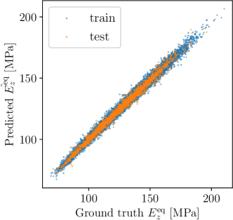
(a) Pin-jointed truss lattice GNN model.

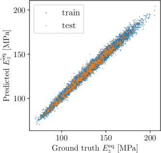
(b) Euler-Bernoulli beam lattice GNN model.

Figure 10: Pin-jointed truss (a) and Euler-Bernoulli beam (b) lattice GNN models. Equivalent stiffness $E_{z}^{\rm eq}$ prediction, where the train and test are represented by blue and orange points, respectively. Note that the diagonal line at $45^{\circ}$ is the perfect prediction.

4.3 Results for Euler-Bernoulli beam lattices

Now we study a different mechanical model, namely a dataset of $N=10\,000$ Euler-Bernoulli beam lattices, with same material and geometrical properties than the pin-jointed truss lattice set counterpart. The same model as the previous section is applied, with same node and edge features, and same architecture—see Table 3 and Figure 9. The validation set is a 15% of this dataset, whereas for the test set, 1000 new samples (10%) are generated separately. All features and targets are scaled with standard normalization, and the training is performed using the parameters displayed in Table 4.

Once the GNN model is trained, the loss function evaluated at both datasets yields $\mathcal{L}_{\rm train}=1.55\cdot 10^{-2}$ and $\mathcal{L}_{\rm test}=2.20\cdot 10^{-2}$. Additionally, the coefficients of determination are $R^{2}_{\rm train}=0.9845$ and $R^{2}_{\rm test}=0.9778$. The predictions are depicted in Figure 10b. Although the prediction of this mechanical model becomes more challenging due to the appearance of shear forces and bending/twisting moments in the (rigid) joints – leading to more equilibrium equations – the GNN model is able to perform accurately on this dataset likewise.

5 Inverse problem

Making use of the GNN surrogate models derived in Section 4, we now present an approach to address the inverse problem i.e., obtaining the lattice structure given a Young’s modulus $E_{z}^{\rm eq,*}$ prescribed by the user. The model is a non-bijective function, thus the inverse problem is ill-posed [23, 24]. Additionally, although a (potentially successful) Newton-Raphson approach to obtain numerically the inputs given an output may be derived – the derivatives of the output w.r.t. the inputs can be computed via automatic differentiation [95] – this approach is still not able to yield the number of nodes, struts and their adjacencies i.e., the graph $\mathcal{G}$—recall that the model inputs are the node and edge features, plus the adjacencies.

Therefore, thanks to the fast evaluations that the surrogate model allows, a database with $100\,000$ samples is rapidly generated to cover a wide range of Young’s moduli $E_{z}^{\rm eq}$. With a sufficient number of samples predicted, several structural choices can yield the same effective property. That is the reason why we introduce the weight (or volume $V$ as defined in Equation (16), since the material stays the same) as an additional variable in this loop, which poses particular interest in structural optimization problems.

Since lightweight structures are pursued, finding the minimum-weight lattice amongst all structures behaving with similar stiffness aims at this objective. To study the maximum-stiffness-minimum-weight configurations, every pair $\{({{V}^{-1}}^{(i)},{E_{z}^{\rm eq}}^{(i)})\}_{i=1}^{N}$ is represented in a 2D scatter plot in Figure 11. Then, a Pareto front [89] is defined given the best stiffness-weight trade-offs, which is depicted in red in such figure.

When requesting a certain Young’s modulus e.g., $E_{z}^{\rm eq,*}=170\,$MPa, a local range $E_{z}^{\rm eq,*}\in\left[E_{\min},E_{\max}\right]$ is defined. Then, a local Pareto front is depicted to look for the lightest solution within that range. In the case of Figure 11, $E_{\min}=169\,$MPa and $E_{\max}=171\,$MPa, thus the lightest solution corresponds to a lattice with $V=7.66\cdot 10^{-3}\,$m³ and $\hat{E_{z}^{\rm eq}}=169.4\,$MPa. We note that the ground-truth effective behavior of such lattice given by the (direct) procedure described in Section 2.4 yields $E_{z}^{\rm eq}=171.0\,$MPa, implying an (absolute) relative error of $0.94\%$.

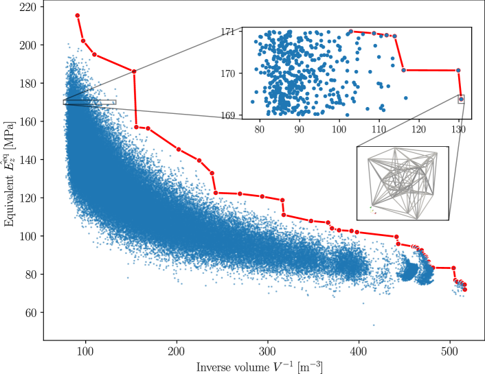
Figure 11: Distribution of inverse volume and equivalent predicted stiffness $(V^{-1},\hat{E_{z}^{\rm eq}})$ of $100\,000$ samples generated with the GNN surrogate model and its optimal Pareto front, in red. Local Pareto fronts can be defined likewise by introducing a range $[E_{\min},E_{\max}]$, set to 169 MPa and 171 MPa in this case in the zoomed in plot. Additionally, the structure with minimum weight of the local Pareto front is represented, with a predicted behavior of $\hat{E_{z}^{\rm eq}}=169.4\,$MPa, whereas the ground-truth property of such lattice yields $E_{z}^{\rm eq}=171.0\,$MPa—implying an (absolute) relative error of $0.94\%$.

6 Conclusions

We developed a surrogate model approach to fast compute effective mechanical properties in pin-jointed truss or Euler-Bernoulli beam (aperiodic) lattices with varied topology. This work represents a framework to efficiently evaluate mechanical properties for many structures without incurring the prohibitive computational cost that classical FE approaches would take. Therefore, this framework is suitable for inverse analysis and, in turn, multi-scale structural optimization problems. The energetically equivalent effective behavior of Young’s modulus is computed with DSM, yielding the ground-truth or high-fidelity solutions used to fit the surrogate model. Although the focus of this study is on predicting the equivalent Young’s modulus, it may be straightforwardly generalized to other mechanical properties such as Poisson’s ratio [86] or the homogenized components of the stiffness tensor [25].

We first derive a DNN surrogate model, which slices the structure into $n_{s}$ portions in the three directions, considering the effective area $A_{i,s}^{\rm eff}$ per slice $s$ and direction $i$. We hypothesize it behaves similarly to a spring-in-series system, hence the slicing and computation of effective areas. Taking all the previous into account, with deep architectures presenting $\sim 10^{5}$ parameters, we can obtain sufficient accuracy for our surrogate model in terms of coefficient of determination $(R^{2}_{\rm test}=0.965)$, successfully predicting the equivalent Young’s modulus per unit volume $\overline{E_{z}^{\rm eq}}$. In other words, by just scanning in three directions a given lattice to compute its effective areas, and weighing the specimen to obtain its volume, the equivalent Young’s modulus can be effectively predicted.

Taking a step further, we build a GNN model to take advantage of the fact that lattices – or any FE mesh – are graphs and exploit the physical meaning of their adjacencies in the learning process. We embed a set of features in the nodes (coordinates) and edges (coordinates of endpoints and length) of the lattices built of the same material. The graph updates performed in the GNN consist of message-passing layers and posterior convolution, which replicate the equilibrium of forces at the nodes. These messages are sent through the elements (trusses, beams), accounting for geometrical (length, cross-sectional area) and material properties (Young’s modulus). Lastly, the pooling layer accounts for the resultant reaction forces in the nodes required to compute the effective behavior $E_{z}^{\rm eq}$. These steps in the GNN are simple matrix operations – all of them linear but the application of activation functions – thus bypassing the classical FE analysis, which requires the assembly and inversion (or factorization) of the stiffness matrix to compute the displacements and reaction forces.

Regarding the results, a GNN with $\sim 10^{3}$ parameters can better predict the effective mechanical behavior $(R^{2}_{\rm test}=0.987$ in case of pin-jointed truss lattices). Note that the GNN model requires two orders of magnitude less parameters than DNN model, achieving even better results in terms of coefficient of determination. We recall that the model is agnostic to the number of nodes and elements that a particular lattice structure presents, which represents a versatile feature [26].

The development of surrogate models allows for fast DoE generation aimed at covering a wide range of (equivalent) mechanical properties. Thus, if a homogeneous block of material with a specific stiffness is required – as in topology optimization algorithms that output functionally graded metamaterials with variable stiffness, see [90, 96] – the most compliant lattice might be found within this generated database. Therefore, an approach to solve inverse problems (macro-to-micro) is derived, making this framework suitable for inverse analysis in multi-scale structural optimization problems. Furthermore, it is possible to find several lattices fulfilling the exact stiffness requirement, leaving room to use another optimization criterion with more variables involved, e.g., the weight of the lattice. We develop global and local Pareto fronts to carry out this multi-objective optimization strategy.

Although the whole study is restricted to linear elastic lattice structures of the same material, we note that this proof of concept represents a building block for considering nonlinear, inelastic effects for multi-material structures, even spanning different scales. This is of great practical relevance to address the data-driven description of deformable solids, with consequent valuable computational time savings.

Declaration of interests

The authors declare that they have no known competing financial interests or personal relationships that could have appeared to influence the work reported in this paper.

References

- [1] L J Gibson and M F Ashby. Cellular solids: structure and properties. Cambridge University Press, 1999.
- [2] N. A. Fleck, V. S. Deshpande, and M. F. Ashby. Micro-architectured materials: past, present and future. In Proceedings of the Royal Society of London A: Mathematical, Physical and Engineering Sciences, volume 466, pages 2495–2516, 2010.
- [3] X Zheng, H Lee, T H Weisgraber, J Shusteff, Mand DeOtte, E B Duoss, J D Kuntz, M M Biener, Q Ge, J A Jackson, S O Kucheyev, N X Fang, and C M Spadaccini. Ultralight, ultrastiff mechanical metamaterials. Science, 344:1373–1377, 2014.
- [4] Nan Yang. Novel structural design method inspired by dna and origami. Results in Engineering, 4:100069, 2019.
- [5] MF Ashby. Overview no. 92: Materials and shape. Acta metallurgica et materialia, 39(6):1025–1039, 1991.
- [6] Michael F Ashby and David Cebon. Materials selection in mechanical design. Le Journal de Physique IV, 3(C7):C7–1, 1993.
- [7] Alejandro R Diaz and Ole Sigmund. A topology optimization method for design of negative permeability metamaterials. Structural and Multidisciplinary Optimization, 41:163–177, 2010.
- [8] Burak Ozbey, Emre Unal, Hatice Ertugrul, Ozgur Kurc, Christian M Puttlitz, Vakur B Erturk, Ayhan Altintas, and Hilmi Volkan Demir. Wireless displacement sensing enabled by metamaterial probes for remote structural health monitoring. Sensors, 14(1):1691–1704, 2014.
- [9] Jacobs Somnic and Bruce W Jo. Homogenization methods of lattice materials. Encyclopedia, 2(2):1091–1102, 2022.
- [10] Jörg Schröder. A numerical two-scale homogenization scheme: the fe2-method. In Plasticity and beyond: microstructures, crystal-plasticity and phase transitions, pages 1–64. Springer, 2014.
- [11] Andrea Tessarin, Mirco Zaccariotto, Ugo Galvanetto, and Domenico Stocchi. A multiscale numerical homogenization-based method for the prediction of elastic properties of components produced with the fused deposition modelling process. Results in Engineering, 14:100409, 2022.
- [12] Herve Moulinec and Pierre Suquet. A fast numerical method for computing the linear and nonlinear mechanical properties of composites. Comptes Rendus de l’Académie des sciences. Série II. Mécanique, physique, chimie, astronomie, 1994.
- [13] Matti Schneider. A review of nonlinear fft-based computational homogenization methods. Acta Mechanica, 232(6):2051–2100, 2021.
- [14] Hooman Danesh, Tim Brepols, and Stefanie Reese. Challenges in two-scale computational homogenization of mechanical metamaterials. PAMM, 23(1):e202200139, 2023.
- [15] Francisco J Montáns, Francisco Chinesta, Rafael Gómez-Bombarelli, and J Nathan Kutz. Data-driven modeling and learning in science and engineering. Comptes Rendus Mécanique, 347(11):845–855, 2019.
- [16] Steven L Brunton, Joshua L Proctor, and J Nathan Kutz. Discovering governing equations from data by sparse identification of nonlinear dynamical systems. Proceedings of the national academy of sciences, 113(15):3932–3937, 2016.
- [17] Quercus Hernandez, Alberto Badias, David Gonzalez, Francisco Chinesta, and Elias Cueto. Deep learning of thermodynamics-aware reduced-order models from data. Computer Methods in Applied Mechanics and Engineering, 379:113763, 2021.
- [18] Ricardo Vinuesa. High-fidelity simulations in complex geometries: Towards better flow understanding and development of turbulence models. Results in Engineering, 11:100254, 2021.
- [19] Maziar Raissi, Paris Perdikaris, and George E Karniadakis. Physics-informed neural networks: A deep learning framework for solving forward and inverse problems involving nonlinear partial differential equations. Journal of Computational physics, 378:686–707, 2019.
- [20] Simone Monaco and Daniele Apiletti. Training physics-informed neural networks: One learning to rule them all? Results in Engineering, 18:101023, 2023.
- [21] Han Gao, Matthew J Zahr, and Jian-Xun Wang. Physics-informed graph neural galerkin networks: A unified framework for solving pde-governed forward and inverse problems. Computer Methods in Applied Mechanics and Engineering, 390:114502, 2022.
- [22] D Di Lorenzo, V Champaney, JY Marzin, C Farhat, and F Chinesta. Physics informed and data-based augmented learning in structural health diagnosis. Computer Methods in Applied Mechanics and Engineering, 414:116186, 2023.
- [23] Mikhail M Lavrentiev, Vladimir Gavrilovich Romanov, and Serge_ Petrovich Shishatskii. Ill-posed problems of mathematical physics and analysis, volume 64. American Mathematical Soc., 1986.
- [24] Jari Kaipio and Erkki Somersalo. Statistical and computational inverse problems, volume 160. Springer Science & Business Media, 2006.
- [25] Hunter T Kollmann, Diab W Abueidda, Seid Koric, Erman Guleryuz, and Nahil A Sobh. Deep learning for topology optimization of 2d metamaterials. Materials & Design, 196:109098, 2020.
- [26] Benjamin Sanchez-Lengeling, Emily Reif, Adam Pearce, and Alexander B Wiltschko. A gentle introduction to graph neural networks. Distill, 6(9):e33, 2021.
- [27] Federico Pichi, Beatriz Moya, and Jan S Hesthaven. A graph convolutional autoencoder approach to model order reduction for parametrized pdes. arXiv preprint arXiv:2305.08573, 2023.
- [28] S Choukir and CV Singh. Role of topology in dictating the fracture toughness of mechanical metamaterials. International Journal of Mechanical Sciences, 241:107945, 2023.
- [29] Yuhao Liu, Jian Yang, Xiaosu Yi, Wenjie Guo, Qingsong Feng, and Dimitrios Chronopoulos. Enhanced vibration suppression using diatomic acoustic metamaterial with negative stiffness mechanism. Engineering Structures, 271:114939, 2022.
- [30] Quanlong Yang, Xieyu Chen, Yanfeng Li, Xueqian Zhang, Yuehong Xu, Zhen Tian, Chunmei Ouyang, Jianqiang Gu, Jiaguang Han, and Weili Zhang. Aperiodic-metamaterial-based absorber. APL Materials, 5(9), September 2017.
- [31] Luca D’Alessandro, Anastasiia O. Krushynska, Raffaele Ardito, Nicola M. Pugno, and Alberto Corigliano. A design strategy to match the band gap of periodic and aperiodic metamaterials. Scientific Reports, 10(1), October 2020.
- [32] Jan-Hendrik Bastek, Siddhant Kumar, Bastian Telgen, Raphaël N. Glaesener, and Dennis M. Kochmann. Inverting the structure–property map of truss metamaterials by deep learning. Proceedings of the National Academy of Sciences, 119(1), December 2021.
- [33] Frank W. Zok, Ryan M. Latture, and Matthew R. Begley. Periodic truss structures. Journal of the Mechanics and Physics of Solids, 96:184–203, November 2016.
- [34] Mark C. Messner. Optimal lattice-structured materials. Journal of the Mechanics and Physics of Solids, 96:162–183, November 2016.
- [35] Lucas R. Meza, Gregory P. Phlipot, Carlos M. Portela, Alessandro Maggi, Lauren C. Montemayor, Andre Comella, Dennis M. Kochmann, and Julia R. Greer. Reexamining the mechanical property space of three-dimensional lattice architectures. Acta Materialia, 140:424–432, November 2017.
- [36] Mingyang Zhang, Zhenyu Yang, Zixing Lu, Baohua Liao, and Xiaofan He. Effective elastic properties and initial yield surfaces of two 3d lattice structures. International Journal of Mechanical Sciences, 138-139:146–158, April 2018.
- [37] Anran Wei, Jie Xiong, Weidong Yang, and Fenglin Guo. Deep learning-assisted elastic isotropy identification for architected materials. Extreme Mechanics Letters, 43:101173, February 2021.
- [38] S. Torquato. Statistical description of microstructures. Annual Review of Materials Research, 32(1):77–111, August 2002.
- [39] Shaoqing Cui, Jinlong Fu, Song Cen, Hywel R. Thomas, and Chenfeng Li. The correlation between statistical descriptors of heterogeneous materials. Computer Methods in Applied Mechanics and Engineering, 384:113948, October 2021.
- [40] Elizabeth Munch. A user’s guide to topological data analysis. Journal of Learning Analytics, 4(2), July 2017.
- [41] Frédéric Chazal and Bertrand Michel. An introduction to topological data analysis: Fundamental and practical aspects for data scientists. Frontiers in Artificial Intelligence, 4, September 2021.
- [42] Dane Taylor, Florian Klimm, Heather A. Harrington, Miroslav Kramár, Konstantin Mischaikow, Mason A. Porter, and Peter J. Mucha. Topological data analysis of contagion maps for examining spreading processes on networks. Nature Communications, 6(1), July 2015.
- [43] Antoine Runacher, Mohammad-Javad Kazemzadeh-Parsi, Daniele Di Lorenzo, Victor Champaney, Nicolas Hascoet, Amine Ammar, and Francisco Chinesta. Describing and modeling rough composites surfaces by using topological data analysis and fractional brownian motion. Polymers, 15(6):1449, March 2023.
- [44] Andrea Vigliotti, Vikram S. Deshpande, and Damiano Pasini. Non linear constitutive models for lattice materials. Journal of the Mechanics and Physics of Solids, 64:44–60, March 2014.
- [45] M. J. Mirzaali, H. Pahlavani, E. Yarali, and A. A. Zadpoor. Non-affinity in multi-material mechanical metamaterials. Scientific Reports, 10(1), July 2020.
- [46] Tianju Xue, Sigrid Adriaenssens, and Sheng Mao. Learning the nonlinear dynamics of mechanical metamaterials with graph networks. International Journal of Mechanical Sciences, 238:107835, January 2023.
- [47] B. Hassani and E. Hinton. A review of homogenization and topology optimization i—homogenization theory for media with periodic structure. Computers & Structures, 69(6):707–717, December 1998.
- [48] B. Hassani and E. Hinton. A review of homogenization and topology opimization II—analytical and numerical solution of homogenization equations. Computers & Structures, 69(6):719–738, December 1998.
- [49] B. Hassani and E. Hinton. A review of homogenization and topology optimization III—topology optimization using optimality criteria. Computers & Structures, 69(6):739–756, December 1998.
- [50] Nicole Coutris, Lonny L Thompson, and Sai Kosaraju. Asymptotic homogenization models for pantographic lattices with variable order rotational resistance at pivots. Journal of the Mechanics and Physics of Solids, 134:103718, January 2020.
- [51] Andrea Braides and Lorenza D’Elia. Homogenization of discrete thin structures. Nonlinear Analysis, 231:112951, June 2023.
- [52] Liang Xu and Zhenghua Qian. Topology optimization and de-homogenization of graded lattice structures based on asymptotic homogenization. Composite Structures, 277:114633, December 2021.
- [53] Florian Vladulescu and Dan Mihai Constantinescu. Lattice topology homogenization and crack propagation through finite element analyses. Procedia Structural Integrity, 28:637–647, 2020.
- [54] Oliver K. Johnson, Jarrod M. Lund, and Tyler R. Critchfield. Spectral graph theory for characterization and homogenization of grain boundary networks. Acta Materialia, 146:42–54, March 2018.
- [55] Umberto De Ambroggio, Federico Polito, and Laura Sacerdote. On dynamic random graphs with degree homogenization via anti-preferential attachment probabilities. Physica D: Nonlinear Phenomena, 414:132689, December 2020.
- [56] Chaoying Yang, Jie Liu, Kaibo Zhou, Xiaohui Yuan, and Xingxing Jiang. A meta-path graph-based graph homogenization framework for machine fault diagnosis. Engineering Applications of Artificial Intelligence, 121:105960, May 2023.
- [57] Dominik Dold and Derek Aranguren van Egmond. Differentiable graph-structured models for inverse design of lattice materials. Cell Reports Physical Science, page 101586, September 2023.
- [58] Zhongkai Ji, Dawei Li, Wenhe Liao, and Yi Min Xie. AI-aided design of multiscale lattice metastructures for controllable anisotropy. Materials & Design, 223:111254, November 2022.
- [59] Andrew J. Lew, Chi-Hua Yu, Yu-Chuan Hsu, and Markus J. Buehler. Deep learning model to predict fracture mechanisms of graphene. npj 2D Materials and Applications, 5(1), April 2021.
- [60] F. Scarselli, M. Gori, Ah Chung Tsoi, M. Hagenbuchner, and G. Monfardini. The graph neural network model. IEEE Transactions on Neural Networks, 20(1):61–80, January 2009.
- [61] Justin Gilmer, Samuel S. Schoenholz, Patrick F. Riley, Oriol Vinyals, and George E. Dahl. Neural message passing for quantum chemistry, 2017.
- [62] Minsik Seo and Seungjae Min. Graph neural networks and implicit neural representation for near-optimal topology prediction over irregular design domains. Engineering Applications of Artificial Intelligence, 123:106284, August 2023.
- [63] Chunhao Jiang and Nian-Zhong Chen. Graph neural networks (GNNs) based accelerated numerical simulation. Engineering Applications of Artificial Intelligence, 123:106370, August 2023.
- [64] Peerasait Prachaseree and Emma Lejeune. Learning mechanically driven emergent behavior with message passing neural networks. Computers & Structures, 270:106825, October 2022.
- [65] Konstantinos Karapiperis and Dennis M. Kochmann. Prediction and control of fracture paths in disordered architected materials using graph neural networks. Communications Engineering, 2(1), June 2023.
- [66] Roberto Perera and Vinamra Agrawal. Dynamic and adaptive mesh-based graph neural network framework for simulating displacement and crack fields in phase field models. Mechanics of Materials, 186:104789, November 2023.
- [67] Akhil Thomas, Ali Riza Durmaz, Mehwish Alam, Peter Gumbsch, Harald Sack, and Chris Eberl. Materials fatigue prediction using graph neural networks on microstructure representations. Scientific Reports, 13(1), August 2023.
- [68] Marco Maurizi, Chao Gao, and Filippo Berto. Predicting stress, strain and deformation fields in materials and structures with graph neural networks. Scientific Reports, 12(1), December 2022.
- [69] M. Raissi, P. Perdikaris, and G.E. Karniadakis. Physics-informed neural networks: A deep learning framework for solving forward and inverse problems involving nonlinear partial differential equations. Journal of Computational Physics, 378:686–707, February 2019.
- [70] George Em Karniadakis, Ioannis G. Kevrekidis, Lu Lu, Paris Perdikaris, Sifan Wang, and Liu Yang. Physics-informed machine learning. Nature Reviews Physics, 3(6):422–440, May 2021.
- [71] Eric J. Hall, Søren Taverniers, Markos A. Katsoulakis, and Daniel M. Tartakovsky. GINNs: Graph-informed neural networks for multiscale physics. Journal of Computational Physics, 433:110192, May 2021.
- [72] Jiang-Zhou Peng, Nadine Aubry, Yu-Bai Li, Mei Mei, Zhi-Hua Chen, and Wei-Tao Wu. Physics-informed graph convolutional neural network for modeling geometry-adaptive steady-state natural convection. International Journal of Heat and Mass Transfer, 216:124593, December 2023.
- [73] Romrawin Chumpu, Chun-Lin Chu, Tanyakarn Treeratanaphitak, Sanparith Marukatat, and Shu-Han Hsu. Physics-informed graph neural networks accelerating microneedle simulations towards novelty of micro-nano scale materials discovery. Engineering Applications of Artificial Intelligence, 126:106894, November 2023.
- [74] David Dalton, Dirk Husmeier, and Hao Gao. Physics-informed graph neural network emulation of soft-tissue mechanics. Computer Methods in Applied Mechanics and Engineering, 417:116351, December 2023.
- [75] Wendi Liu and Michael J. Pyrcz. Physics-informed graph neural network for spatial-temporal production forecasting. Geoenergy Science and Engineering, 223:211486, April 2023.
- [76] Rajeev Das and Azzedine Soulaimani. Non-deterministic methods and surrogates in the design of rockfill dams. Applied Sciences, 11(8):3699, April 2021.
- [77] Hannah Jordan. A Non-Deterministic Deep Learning Based Surrogate for Ice Sheet Modelling. Master of Science (MS) Thesis, Department of Computer Science, University of Montana, 2022.
- [78] Nora Luethen, Stefano Marelli, and Bruno Sudret. A spectral surrogate model for stochastic simulators computed from trajectory samples. Computer Methods in Applied Mechanics and Engineering, 406:115875, March 2023.
- [79] Yuan Feng, Di Wu, Mark G. Stewart, and Wei Gao. Past, current and future trends and challenges in non-deterministic fracture mechanics: A review. Computer Methods in Applied Mechanics and Engineering, 412:116102, July 2023.
- [80] Mohammad Amin Hariri-Ardebili and Golsa Mahdavi. Generalized uncertainty in surrogate models for concrete strength prediction. Engineering Applications of Artificial Intelligence, 122:106155, June 2023.
- [81] Xiaoxiao Wang, Haofeng Chen, and Fuzhen Xuan. Neural network-assisted probabilistic creep-fatigue assessment of hydrogenation reactor with physics-based surrogate model. International Journal of Pressure Vessels and Piping, 206:105051, December 2023.
- [82] Shaoyi Cheng, Bisheng Wu, Ming Zhang, Xi Zhang, Yanhui Han, and Robert G. Jeffrey. Surrogate modeling and global sensitivity analysis for the simultaneous growth of multiple hydraulic fractures. Computers and Geotechnics, 162:105709, October 2023.
- [83] Syifaul Huzni, Israr BM Ibrahim, Syarizal Fonna, and Ramana Pidaparti. Physics-based surrogate model for reinforced concrete corrosion simulation. Results in Engineering, 16:100659, 2022.
- [84] A. Bowyer. Computing dirichlet tessellations. The Computer Journal, 24(2):162–166, February 1981.
- [85] D. F. Watson. Computing the n-dimensional delaunay tessellation with application to voronoi polytopes. The Computer Journal, 24(2):167–172, February 1981.
- [86] Ismael Ben-Yelun, Guillermo Gómez-Carano, Francisco J San Millán, Miguel Ángel Sanz, Francisco Javier Montáns, and Luis Saucedo-Mora. Gam: General auxetic metamaterial with tunable 3d auxetic behavior using the same unit cell boundary connectivity. Materials, 16(9):3473, 2023.
- [87] Omer San, Romit Maulik, and Mansoor Ahmed. An artificial neural network framework for reduced order modeling of transient flows. Communications in Nonlinear Science and Numerical Simulation, 77:271–287, 2019.
- [88] Christopher M Bishop and Nasser M Nasrabadi. Pattern recognition and machine learning, volume 4. Springer, 2006.
- [89] Stephen P Boyd and Lieven Vandenberghe. Convex optimization. Cambridge university press, 2004.
- [90] Ismael Ben-Yelun, Luis Saucedo-Mora, Miguel Ángel Sanz, José María Benítez, and Francisco Javier Montans. Topology optimization approach for functionally graded metamaterial components based on homogenization of mechanical variables. Computers & Structures, 289:107151, 2023.
- [91] Janusz S Przemieniecki. Theory of matrix structural analysis. Courier Corporation, 1985.
- [92] Kurt Hornik, Maxwell Stinchcombe, and Halbert White. Multilayer feedforward networks are universal approximators. Neural networks, 2(5):359–366, 1989.
- [93] Günter Klambauer, Thomas Unterthiner, Andreas Mayr, and Sepp Hochreiter. Self-normalizing neural networks. Advances in neural information processing systems, 30, 2017.
- [94] Timothy Dozat. Incorporating nesterov momentum into adam. 2016.
- [95] Atilim Gunes Baydin, Barak A Pearlmutter, Alexey Andreyevich Radul, and Jeffrey Mark Siskind. Automatic differentiation in machine learning: a survey. Journal of Marchine Learning Research, 18:1–43, 2018.
- [96] Luis Saucedo-Mora, Ismael Ben-Yelun, Hugo García-Modet, Miguel Ángel Sanz-Gómez, and Francisco Javier Montans. The updated properties model (upm): A topology optimization algorithm for the creation of macro–micro optimized structures with variable stiffness. Finite Elements in Analysis and Design, 223:103970, 2023.