Role of Brownian motion and Néel relaxations
in Mössbauer spectra of magnetic liquids

Abstract

The absorption cross section of Mössbauer radiation in magnetic liquids is calculated, taking into consideration both translational and rotational Brownian motion of magnetic nanoparticles. Stochastic reversals of their magnetization are also regarded in the absence of external magnetic field. The role of Brownian motion in ferrofluids is considered in the framework of the diffusion theory, while for the magnetorheological fluids with large nanoparticles it is done in the framework of the Langevin’s approach. For rotation we derived the equation analogous to Langevin’s equation and gave the corresponding correlation function. In both cases the equations for rotation are solved in the approximation of small rotations during lifetime of the excited state of Mössbauer nuclei. The influence of magnetization relaxations is studied with the aid of the Blume-Tjon model.

I Introduction

Suspensions of magnetic nanoparticles (MNPs) attract great attention due to their numerous applications in technique, medicine and biology [1-17]. It is provided by large magnetic moment of MNPs, which allows to manipulate them by moderate magnetic fields. Depending on the dimensions of MNPs, they can be divided into magnetorheological fluids formed by MNPs with the diameter of the order of $1\mu$m and ferrofluids with dimensions of MNPs $\sim 10$ nm (see, e.g., Brazil ). Viscosity of the magnetorheological liquids, being subjected to the magnetic field, enormously increases, so that they may even transform into a solid body. This property gives possibility to use such suspensions in dampers, brakes and clutches Wang .

Ferrofluids are widely used in computers, loudspeakers, semiconductors, motion controllers, sensors, ink-jet printers, seals, bearings, stepper motors, etc [1-8].

In medicine ferrofluids are employed in hyperthermia Mody , for drug delivering to local ill regions of the body and as contrast agents in magnetic resonance imaging (MRI) med . Recently, much more progressive method of magnetic particle imaging (MPI) was developed for visualizing MNPs in humans and animals [11-15]. The advantage of MPI is that it is more fast, quantitative, and sensitive than MRI.

Note that MNPs are always coated with a polymer shell to prevent their agglomeration in a solution. The commercial ferrofluids are predominantly based on magnetite Fe₃0₄ particles.

Usually MNPs have single easy-magnetization axis $\zeta$ and their magnetization ${\bf M}$ tends to be oriented along it or in the opposite direction, keeping the constant value $|{\bf M}|$. The anisotropy potential energy of such particles in the absence of external magnetic fields, versus the angle $\Theta$ between ${\bf M}$ and axis $\zeta$, is represented by two potential wells at $\Theta=0$ and $\pi$, separated by the potential barrier:

$$E=K_{\textrm{\scriptsize{eff}}}V\sin^{2}\Theta,$$ (1)

where $K_{\textrm{\scriptsize{eff}}}$ denotes the effective magnetic anisotropy, $V$ the particle volume. The magnetization, oscillating in one of the potential wells, from time to time gets sufficient energy to jump over the barrier into the neighboring well. In the symmetric potential (1) the magnetization reversals occur with equal rate $w=1/\tau$ in both sides, where the relaxation time $\tau_{N}$ is determined by Néel’s formula Neel

$$\tau_{N}=\tau_{0}\exp{\left(\frac{K_{\textrm{\scriptsize{eff}}}V}{kT}\right)}$$ (2)

with the constant factor $\tau_{0}\sim 10^{-9}-10^{-13}s^{-1}$ (see, e.g., Landers ).

Effectiveness of the MNPs in different applications strongly depends on such parameters as the Nèel relaxation time and Brownian rotational relaxation time of MNPs as well as their relation to temperature and viscosity of the carrier fluid. The Mössbauer spectroscopy is the most powerful method allowing us to determine all such characteristics. Soon after discovery the Mössbauer effect has been applied for investigation of the Brownian motion of nanoparticles in liquids [18-26]. Foundation of these studies has been laid by Singwi and Sjölander Singwi , who expressed the absorption cross section of Mössbauer rays by chaotically moving nanoparticle in terms of the Van Hove auto-correlation function. Having described the translational motion of the Brownian particle by diffusion equation, they found that the broadening of Mössbauer line linearly depends on the ratio of temperature $T$ and viscosity of the liquid $\eta$. This conclusion was supported experimentally for small nanoparticles [18-24]. But somewhat later for large particles it was observed considerable curvature of the line, which was explained theoretically in Refs. K ; B2 , where the Brownian motion was described by means of the stochastic Langevin’s equation.

For the first time the role of the Brownian rotation was analyzed by Zatovskiǐ Zat , who found most strict solution for the absorption cross section. In Ref. Dz1 this task has been solved in small-angle approximation, taking into account that during the lifetime of the excited Mössbauer nucleus the root mean-square angle of the Brownian rotation is usually much less than unity. Such simple calculations were expanded to the case of ellipsoidal Brownian particles in Ref. Dz2 . Another more cumbersome approach to the problem was developed in Ref. Af .

Besides, manifestation of the Néel relaxations along with the Brownian motion in Mössbauer spectra was studied in Ref. Dz3 , whereas Landers et al. [17] seem to be the first who observed the Mössbauer spectra in ferrofluids. Interesting experimental results have been also reported in Refs.[33-36].

In this paper we research in much more detail the impact of Brownian rotation together with translational diffusion on the shape of Mössbauer spectra. In particular, for the first time the Brownian rotation of large nanoparticles will be regarded in the framework of Langevin’s formalism on the same footing as the translational motion.

For ferrofluids we shall apply a simplest relaxation model, when the magnetization vector of the particle ${\bf M}(t)$ makes stochastic jumps between the values ${\bf M}$ and $-{\bf M}$ along the easy axis $\zeta$. Respectively, the magnetic field at the nucleus, being antiparallel to ${\bf M}(t)$, takes the values ${\bf h}_{0}(t)={\bf h}_{0}f(t)$ with $f(t)=\pm 1$. The magnetic field ${\bf h}_{0}$ causes splitting of the nuclear sublevels giving rise to a Zeeman sextet. For generality we adopt that along the field ${\bf h}_{0}$ there is an electric field gradient, which ensures a quadrupole splitting of the lines. This model was previously applied to calculations of Mössbauer spectra by Blume and Tjon Blume .

II Basic equations

In order to separate the translational and rotational motion we first introduce the coordinate frame $\{x,\;y,\;z\}$ with the origin in the center of the particle and axis $z$ along the beam of incident $\gamma$-quanta. In addition, we introduce the frame $\{\xi,\;\eta,\;\zeta\}$ with axis $\zeta$ along the easy-magnetization axis of the particle. Position of the Mössbauer nucleus ⁵⁷Fe in the laboratory frame $\{x_{L},\;y_{L},\;z_{L}\}$ is determined by the radius-vector

$${\bf X}={\bf R}+{\bf r}+{\bf u},$$ (3)

where the vector ${\bf R}$ indicates position of the center of the Brownian particle, ${\bf r}$ specifies the equilibrium position of the nucleus in the frame $\{x,\;y,\;z\}$, and ${\bf u}$ is the displacement from this cite.

Random reversals of the magnetization ${\bf M}$ and the Brownian motion are independent processes. Therefore the absorption cross section of $\gamma$-quanta with the energy $E=\hbar\omega$ and wave vector ${\bm{\kappa}}$ by the Mössbauer nucleus ⁵⁷Fe, embedded in the Brownian particle, may be written as Dz3

$$\sigma_{a}(\omega)=\frac{\sigma_{0}\Gamma_{a}}{2}e^{-2W}$$ (4)

$$\times\mbox{Re}\int_{0}^{\infty}\frac{dt}{\hbar}e^{i(\omega-\omega_{a})t-\Gamma_{a}t/2\hbar}G_{B}({\bm{\kappa}},t)G_{N}(t),$$

where $\sigma_{0}$ is the resonant value of the absorption cross section of $\gamma$-quanta by a fixed nucleus in the absence of the hyperfine structure, $E_{a}=\hbar\omega_{a}$ and $\Gamma_{a}$ are the energy and width of the resonant level of the absorbing nucleus, $e^{-2W}$ is the Debye-Waller factor, $G_{B}({\bm{\kappa}},t)$ denotes the Fourier-transform of the classical autocorrelation function for the Brownian motion, $G_{N}(t)$ the correlation function for the Néel relaxations of magnetization.

This cross section is to be averaged over the energy distribution of $\gamma$-quanta emitted by a source without recoil

$$w_{e}(E)=\frac{2\pi}{\Gamma_{e}}\frac{1}{(E-E_{e}-s)^{2}+(\Gamma_{e}/2)^{2}},$$ (5)

where $s=vE_{e}/c$ denotes the Doppler shift for a source, moving with the velocity $v$ relative to an absorber. Then experimentally measured cross section takes the form

$$\sigma_{a}(s)=\frac{\sigma_{0}\Gamma_{a}}{2}e^{-2W}$$ (6)

$$\times\mbox{Re}\int_{0}^{\infty}\frac{dt}{\hbar}e^{ist/\hbar-\Gamma_{0}t/2\hbar}G_{B}({\bm{\kappa}},t)G_{N}(t),$$

where $\Gamma_{0}=\Gamma_{e}+\Gamma_{a}$ means the width observed when any broadening due to Brownian motion or Néel relaxations is absent.

For spherical particles the translational and rotational Brownian motions are separated, so that

$$G_{B}({\bm{\kappa}},t)=G_{t}({\bm{\kappa}},t)G_{r}({\bm{\kappa}},t),$$ (7)

where $G_{t}({\bm{\kappa}},t)$ and $G_{r}({\bm{\kappa}},t)$ are the Fourier transforms of the correlation functions for translational motion and rotation, respectively.

III Correlation functions

In this section we shall give the correlation functions for the translational and rotational Brownian motion of spherical nanoparticles in a liquid, provided by corresponding diffusion equations. Besides, the correlator responsible for the Néel relaxations of the MNPs magnetization, derived in Ref. Blume , will be reproduced below in somewhat changed form.

3.1 Translational Brownian motion

For the translational Brownian motion, described by simple diffusion equation, the correlation function has the form Singwi

$$G^{t}_{s}({\bf R},t)=(4\pi D_{t}|t|)^{-3/2}\exp[-R^{2}/4D_{t}|t|].$$ (8)

Here we suppose that at the initial moment $t=0$ the particle is located in the origin of the laboratory frame. The Fourier-transform of the function (8) reads

$$G_{s}^{t}({\bm{\kappa}},t)=\exp(-\kappa^{2}D_{t}|t|).$$ (9)

As a result, the broadening of the Mössbauer line caused by translational diffusion of a spherical nanoparticle is given by Singwi

$$\Delta\Gamma_{t}=2\hbar\kappa^{2}D_{t},$$ (10)

where the translational diffusion coefficient

$$D_{t}=\frac{kT}{6\pi\eta a_{h}},$$ (11)

$\eta$ is the viscosity coefficient of the liquid, $a_{h}$ the hydrodynamic radius of the nanoparticle being a sum of the core radius $a_{c}$ and a thickness of its coating $d$.

3.2 Brownian rotation

The mean-square angle of rotation $\Delta_{r}^{2}$ of the Brownian particle in a liquid during time $t$ is determined by Einstein’s formula Ein

$$\Delta^{2}_{r}=2D_{r}t,$$ (12)

depending on the rotation diffusion coefficient

$$D_{r}=\frac{kT}{8\pi\eta a_{h}^{3}},$$ (13)

where $a_{h}$ is the hydrodynamic radius of the particle.

Let us estimate the $\Delta^{2}_{r}$ for rotation during the time $t$ of the order of the lifetime $\tau_{N}=\hbar/\Gamma_{a}=141$ ns for ⁵⁷Fe. We take the parameters of the experiment Landers , which correspond to maximal value of $\Delta^{2}_{r}$: $a_{h}=7$ nm and $\eta=22.5$ cp (viscosity of the 70% glycerol solution at $T=293$ K). In this case $\Delta^{2}_{r}\approx 4\cdot 10^{-3}$. In all other measurements Landers , corresponding to lower temperatures and larger particles, $\Delta^{2}_{r}$ is much less. Thus, we can really treat the Brownian rotation in the small-angle approximation.

The Fourier-transform of the rotational correlation function is calculated with the aid of the probability density $W({\bf n},{\bf n}_{0};t)$ of the Brownian rotation from ${\bf n}_{0}$ to ${\bf n}$ during time $t$:

$$G_{s}^{r}({\bm{\kappa}},t)=\int d{\bf n}W({\bf n},{\bf n}_{0};t)e^{i{\bm{\kappa}}({\bf n}-{\bf n}_{0})r},$$ (14)

where orientation of the unit vectors ${\bf n}_{0}={\bf r}(0)/r$ and ${\bf n}={\bf r}(t)/r$ in the frame $\{x,\;y,\;z\}$ are determined by the spherical angles $\theta_{0},\varphi_{0}$ and $\theta,\varphi$, respectively. The function $W({\bf n},{\bf n}_{0};t)$ is looked for as a solution of the rotational diffusion equation Leon

$$\frac{\partial W}{\partial t}=D_{r}\left[\frac{\partial^{2}W}{\partial\theta^{2}}+\cot\theta\frac{\partial W}{\partial\theta}+\frac{1}{\sin^{2}\theta}\frac{\partial^{2}W}{\partial\varphi^{2}}\right]$$ (15)

with the initial condition

$$W({\bf n},{\bf n}_{0};0)=\delta({\bf n}-{\bf n}_{0}).$$ (16)

The probability of all possible events equals unity, therefore the probability density is normalized as

$$\int_{0}^{\pi}\sin\theta d\theta\int_{0}^{2\pi}d\varphi W({\bf n},{\bf n}_{0};t)=1.$$ (17)

Let us introduce one more frame $x^{\prime},\;y^{\prime},\;z^{\prime}$, whose axis $z^{\prime}$ is directed along ${\bf n}_{0}$. The orientation of the vector ${\bf n}$ in this frame is determined by the spherical angles $\vartheta,\phi$. In the approximation of small Brownian rotations, when

$$({\bf n}-{\bf n}_{0})^{2}\approx\vartheta^{2}<<1,$$ (18)

the basic equation (15) transforms to

$$\frac{\partial W}{\partial t}=D_{r}\left[\frac{\partial^{2}W}{\partial\vartheta^{2}}+\frac{1}{\vartheta}\frac{\partial W}{\partial\vartheta}+\frac{1}{\vartheta^{2}}\frac{\partial^{2}W}{\partial\phi^{2}}\right].$$ (19)

Notice that the same form has the equation, which describes diffusion of the point-like particle on the plane, expressed in polar coordinates with the radial coordinate $\vartheta$ and azimute angle $\phi$. Hence, a solution of Eq. (19), satisfying the initial condition (16), is

$$W({\bf n},{\bf n}_{0};t)=\frac{1}{4\pi D_{r}|t|}\exp\left(-\frac{\vartheta^{2}}{4D_{r}|t|}\right).$$ (20)

From here we see that the mean-square rotation angle is really determined by Eq. (12).

In order to calculate the Fourier-transform of $W({\bf n},{\bf n}_{0};t)$ we shall express the components $n_{x},\;n_{y},\;n_{z}$ of the of unit vector ${\bf n}$ in spherical angles:

$$n_{x}=\sin\theta\cos\varphi,\quad n_{y}=\sin\theta\sin\varphi,\quad n_{z}=\cos\theta.$$ (21)

Simple calculation gives

$$({\bf n}-{\bf n}_{0})^{2}=(\theta-\theta_{0})^{2}+\sin^{2}\theta_{0}(\varphi-\varphi_{0})^{2}.$$ (22)

Comparing (18) with (22) we rewrite (20) as

$$W({\bf n},{\bf n}_{0};t)=\frac{1}{4\pi D_{r}|t|}\qquad\qquad$$ (23)

$$\times\exp\left(-\frac{(\theta-\theta_{0})^{2}}{4D_{r}|t|}\right)\exp\left(-\frac{\sin^{2}\theta_{0}(\varphi-\varphi_{0})^{2}}{4D_{r}|t|}\right).$$

Then starting from the formula

$$G_{s}^{r}({\bm{\kappa}},t)=\int_{-\infty}^{\infty}\sin\theta d\theta\exp[-i\kappa r\sin\theta_{0}(\theta-\theta_{0})]$$

$$\times\int_{-\infty}^{\infty}d\varphi W({\bf n},{\bf n}_{0};t),$$ (24)

we arrive at the Fourier-transform of the rotation correlation function:

$$G_{s}^{r}({\bm{\kappa}},t)=\exp\left[-\kappa^{2}D_{r}r^{2}\sin^{2}\theta_{0}|t|\right].$$ (25)

3.3 Magnetization relaxations

Following Ref. Blume we suppose that there is an electric field gradient along the magnetic field ${\bf h}_{0}$ at the nucleus ⁵⁷Fe. The constant field ${\bf h}_{0}$ gives rise to Zeeman splitting of sublevels $1/2,M_{g}$ and $3/2,M_{e}$ of the ground and excited nuclear states, respectively. Here $M_{g}$ and $M_{e}$ are the projections of the nuclear spin on the direction ${\bf h}_{0}$. In the fluctuating field ${\bf h}_{0}(t)$ the Mössbauer spectrum is described by the correlator $G_{N}(t)$ Blume

$$G_{N}(t)=\sum_{j=1}^{6}J_{j}(\beta)\exp[-iQ(3M_{e}^{2}-15/4)t/\hbar]$$ (26)

$$\times\left(\exp\left[i\alpha_{j}\int_{0}^{t}f(t^{\prime})dt^{\prime}\right]\right)_{av},$$

where $(...)_{av}$ implies the stochastic averaging, $f(t)=\pm 1$, the parameter $Q$ determines a quadrupole shift of the lines, the factors $J_{j=M_{g}\to M_{e}}(\beta)$ are relative intensities of the Zeeman sextet:

$$J_{1=-1/2\to-3/2}(\beta)=J_{6=1/2\to 3/2}(\beta)=\frac{3}{16}(1+\cos^{2}\beta),$$

$$J_{2=-1/2\to-1/2}(\beta)=J_{5=1/2\to 1/2}(\beta)=\frac{1}{4}\sin^{2}\beta,\qquad$$ (27)

$$J_{3=-1/2\to 1/2}(\beta)=J_{4=1/2\to-1/2}(\beta)=\frac{1}{16}(1+\cos^{2}\beta),$$

depending on the angle $\beta$ between the wave vector of $\gamma$-quanta ${\bm{\kappa}}$ and magnetization $+{\bf M}$. Here the lines of the Zeeman sextet are numerated in the order of growing energy. In the absence of external magnetic fields, when the particles are oriented randomly, the averaged relative intensities of the lines $J_{i}=\langle J_{i}(\beta)\rangle$ are

$$J_{1}=J_{6}=\frac{3}{12},\;\;J_{2}=J_{5}=\frac{2}{12},\;\;J_{3}=J_{4}=\frac{1}{12}.$$ (28)

Then the stochastic averaging results in Blume

$$\left(\exp\left[i\alpha_{j}\int_{0}^{t}f(t^{\prime})dt^{\prime}\right]\right)_{av}=$$ (29)

$$=(\cos x_{j}wt+x_{j}^{-1}\sin x_{j}wt)\exp(-wt),$$

with parameters

$$x_{j}=[(\alpha_{j}/w)^{2}-1]^{1/2},$$

$$\alpha_{j}=\alpha_{eg}=(g_{g}M_{g}-g_{e}M_{e})\mu_{N}h_{0}/\hbar,$$ (30)

depending on the nuclear magneton $\mu_{N}$ and gyromagnetic ratios $g_{g}$, $g_{e}$ of the ground and excited states, respectively. From now on, for brevity, we shall omit the exponential in Eq. (29), associated with the quadrupole splitting. Once $Q\neq 0$, in all equations below the Doppler shift $s$ is to be replaced by $s-Q(3M_{e}^{2}-15/4)$.

IV Absorption cross section

Substituting (9), (25) and (29) into (6) one finds the absorption cross section

$$\sigma_{a}(s)=\frac{\sigma_{0}\Gamma_{a}}{4}e^{-2W}\mbox{Re}\sum_{j=1}^{6}J_{j}\left[\left(1-\frac{i}{x_{j}}\right)\frac{i}{s+x_{j}\hbar w+i\Gamma_{\textrm{\scriptsize{eff}}}/2}+\left(1+\frac{i}{x_{j}}\right)\frac{i}{s-x_{j}\hbar w+i\Gamma_{\textrm{\scriptsize{eff}}}/2}\right],$$ (31)

where the effective width

$$\Gamma_{\textrm{\scriptsize{eff}}}=\Gamma_{0}+\Delta\Gamma_{B}+\Delta\Gamma_{N},$$ (32)

$\Delta\Gamma_{N}=2\hbar w$ is a broadening due to the Néel relaxations, while the Brownian broadening is given by a sum

$$\Delta\Gamma_{B}=\Delta\Gamma_{t}+\Delta\Gamma_{r}({\bf r})$$ (33)

with the rotational contribution

$$\Delta\Gamma_{r}({\bf r})=2\hbar\kappa^{2}D_{r}r^{2}\sin^{2}\theta_{0},$$ (34)

depending on the coordinates of the Mössbauer nucleus ⁵⁷Fe.

For uniform distribution of these nuclei in nanoparticle the averaged cross section is defined by

$$\langle\sigma_{a}(s)\rangle=\frac{3}{2a_{c}^{3}}\int_{0}^{a_{c}}r^{2}dr\int_{0}^{\pi}\sigma_{a}(s)\sin\theta_{0}d\theta_{0}.$$ (35)

Having substituted here the expression (31) we introduce new variables $\xi=\cos\theta_{0}$ and $\rho=r/a_{c}$ to obtain

$$\langle\sigma_{a}(s)\rangle=\frac{3\sigma_{0}\Gamma_{a}}{4}e^{-2W}\mbox{Re}\sum_{j=1}^{6}J_{j}\int_{0}^{1}\rho^{2}d\rho$$ (36)

$$\times\left[\left(1-\frac{i}{x_{j}}\right)I_{j}^{+}(\rho)+\left(1+\frac{i}{x_{j}}\right)I_{j}^{-}(\rho)\right],$$

where $I_{j}^{\pm}(\rho)$ stands for the integral

$$I_{j}^{\pm}(\rho)=\int_{0}^{1}\frac{d\xi}{A_{j}^{\pm}(\rho)-B(\rho)\xi^{2}}$$ (37)

with

$$B=i\hbar\kappa^{2}D_{r}a_{c}^{2}\rho^{2}=(3i/8)\Delta\Gamma_{t}(a_{c}/a_{h})^{2}\rho^{2}$$ (38)

and

$$A_{j}^{\pm}=s\pm x_{j}w+i(\Gamma_{0}+\Delta\Gamma_{t}+\Delta\Gamma_{N})/2+B.$$ (39)

Trivial integration gives

$$I_{j}^{\pm}(\rho)=\frac{1}{\sqrt{A_{j}^{\pm}B}}\operatorname{Arth}\left({\sqrt{B/A_{j}^{\pm}}}\right).$$ (40)

In the case of slow relaxations, when $w<<|\alpha_{j}|$ and respectively $x_{j}>>1$ as well as $x_{j}w\approx\alpha_{j}$, the cross section reduces to Zeeman’s pattern with broadened lines:

$$\langle\sigma_{a}(s)\rangle=\frac{\sigma_{0}\Gamma_{a}}{2}e^{-2W_{a}}\mbox{Re}\sum_{j=1}^{6}J_{j}$$ (41)

$$\times\int_{0}^{1}\rho^{2}d\rho\frac{1}{\sqrt{A_{j}B}}\operatorname{Arth}\left(\sqrt{B/A_{j}}\right),$$

where $B$ is again determined by formula (38), while $A_{j}$ takes the form

$$A_{j}=s-\hbar\alpha_{j}+i(\Gamma_{0}+\Delta\Gamma_{t}+\Delta\Gamma_{N})/2+B.$$ (42)

In the opposite limit of very rapid relaxations as $w>>|\alpha_{j}|$ the nucleus only feels an average zero magnetic field. In this case the cross section collapses to single line

$$\langle\sigma_{a}(s)\rangle=\frac{3\sigma_{0}\Gamma_{a}}{2}e^{-2W_{a}}\mbox{Re}\int_{0}^{1}\rho^{2}d\rho$$ (43)

$$\times\frac{1}{\sqrt{AB}}\operatorname{Arth}\left(\sqrt{B/A}\right),$$

where $B$ remains the same, while $A$ becomes

$$A=s+i(\Gamma_{0}+\Delta\Gamma_{t})/2+B.$$ (44)

Note also that the same expression (43) describes the Mössbauer spectra of nonmagnetic Brownian particles.

The formulas considerably simplify, if we average only $\Delta\Gamma_{r}({\bf r})$ instead of the whole cross section (31). Then

$$\langle r^{2}\sin^{2}\theta_{0}\rangle=0.4a_{c}^{2}$$ (45)

and

$$\langle\Delta\Gamma_{r}({\bf r})\rangle=0.6\hbar\kappa^{2}D_{t}(a_{c}/a_{h})^{2}.$$ (46)

In this case the averaged cross section is determined by the same formula (31) but with the Brownian broadening $\Delta\Gamma_{B}$ replaced by

$$\langle\Delta\Gamma_{B}\rangle=2\hbar\kappa^{2}D_{t}[1+0.3(a_{c}/a_{h})^{2}].$$ (47)

As to the cross section (43, it reduces to

$$\langle\sigma_{a}(s)\rangle=\frac{\sigma_{0}\Gamma_{a}}{4}e^{-2W_{a}}\frac{\Gamma_{0}+\langle\Delta\Gamma_{B}\rangle}{s^{2}+(\Gamma_{0}+\langle\Delta\Gamma_{B}\rangle)^{2}/4}.$$ (48)

If a contribution of the rotation is neglected, Eq. (48) coincides with the result of Singwi and Sjolander Singwi .

The role of rotational diffusion is illustrated by Fig.1, where all the cross sections are calculated in units $(3\sigma_{0}\Gamma_{a}/2)e^{-2W}$ as a function of the dimensionless parameter $2s/(\Gamma_{0}+\Delta\Gamma_{t})$ for the case, when $\Delta\Gamma_{t}=4\Gamma_{0}$ and $a_{c}=a_{h}$. The cross section (43) is drawn by the solid line. The Singwi-Sjolander’s curve, given by Eq. (48) with rotational contribution $\langle\Delta\Gamma_{r}({\bf r})\rangle=0$, by the dashed one. In addition, the approximate curve (48) with $\langle\Delta\Gamma_{B}\rangle=2.6\hbar\kappa^{2}D_{t}$, is represented by the dash-dotted line. It is seen that it surprisingly well approximates the exact result (43).

Figure 1: Dependance of the absorption cross sections on the Doppler shift $s$, expressed in units $(\Gamma_{0}+\Delta\Gamma_{t})/2$. The cross section calculated by Eq. (43) is drawn by solid line, the result of Singwi and Sjolander Singwi by dashed one, the approximate expression (48) by dash-dotted.

V Approach based on Langevin’s equation

The correlation function (8) is not valid at small times. More correctly self-diffusion is described by the correlation function Singwi ; Chan

$$G_{t}({\bf R},t)=[2\pi\rho_{t}(t)]^{-3/2}\exp\left[-\frac{R^{2}}{2\rho_{t}(t)}\right],$$ (49)

where

$$\rho_{t}(t)=\frac{2D_{t}}{\beta_{t}}[\beta_{t}t-1+\exp(-\beta_{t}t)],$$ (50)

with

$$\beta_{t}=6\pi a\eta/m=\frac{kT}{D_{t}m}.$$ (51)

The parameter $\beta_{t}^{-1}$ means the characteristic (relaxation) time for the Brownian translational motion.

At $t>>\beta_{t}^{-1}$ the correlation functions (8) and (49) coincide. In the opposite limit of $t<<\beta_{t}^{-1}$ an employment of diffusion approach leads to paradox, remarked in Ref. Chuev1 . Really, from the diffusion equation it follows that at $t\geq 0$ the mean-square displacement $\langle x^{2}\rangle=2D_{t}t$, and therefore the root mean-square velocity along the axis $x$, given by ${\sqrt{\langle v^{2}_{x}\rangle}}=\sqrt{2D_{t}/t}$, tends to infinity if $t\to 0$. At the same time, in correspondence with (50), at $t<<\beta_{t}^{-1}$ the mean-square displacement $\langle x^{2}\rangle=D_{t}\beta_{t}t^{2}$, hence $\sqrt{\langle v^{2}_{x}\rangle}=\sqrt{D_{t}\beta_{t}}=(kT/m)^{1/2}$. Thus, the mean kinetic energy of the Brownian particle $\bar{E}_{\textrm{\scriptsize{kin}}}$ at $t\to 0$ occurs to be determined by the same expression as $\bar{E}_{\textrm{\scriptsize{kin}}}$ for the molecules of the ideal gas:

$$\bar{E}_{\textrm{\scriptsize{kin}}}=3kT/2.$$ (52)

The function (49) was derived by Chandrasekhar Chan from Langevin’s equation

$$\frac{d^{2}{\bf R}}{dt^{2}}=-\beta_{t}\frac{d{\bf R}}{dt}+{\bf F}_{\textrm{\scriptsize{rand}}}(t)/m.$$ (53)

Here on the right-hand side the first term is responsible for the dynamical friction, ${\bf F}_{\textrm{\scriptsize{rand}}}(t)/m$ are random forces acting on the Brownian particle.

Let us find now analogous correlation function for the rotational Brownian motion. For this aim we shall first derive the equation similar to Eq. (53), starting from well-known relationship for the angular momentum ${\bf L}$ of the rotating rigid body and the total torque ${\bf K}$ acting on it Landau :

$$\frac{d{\bf L}}{dt}={\bf K}.$$ (54)

We take into account that the angular momentum for a rigid sphere of the radius $a$ is bound to its angular frequency of rotation ${\bm{\omega}}$ by

$${\bf L}=\mathfrak{J}{\bm{\omega}},$$ (55)

where the inertia moment of the sphere

$$\mathfrak{J}=0.4ma_{h}^{2}.$$ (56)

The ${\bf K}$ equals a sum of the friction torque Kirch

$${\bf K}_{\textrm{\scriptsize{fr}}}=-8\pi\eta a_{h}^{3}{\bm{\omega}}.$$ (57)

and torques ${\bf K}_{\textrm{\scriptsize{rand}}}(t)$ due to random forces.

Inserting (55), (57) into (54) one gets the equation, governing the stochastic rotational motion:

$$\frac{d{\bm{\omega}}}{dt}=-\beta_{r}{\bm{\omega}}+{\bf K}_{\textrm{\scriptsize{rand}}}(t)/\mathfrak{J},$$ (58)

where

$$\beta_{r}=\frac{20\pi\eta a_{h}}{m}=\frac{5}{2}\frac{kT}{D_{r}ma_{h}^{2}}.$$ (59)

Keeping in mind that for small rotations ${\bm{\omega}}$ is perpendicular to ${\bf n}_{0}$ and equals $\omega=d\vartheta/dt$, we transform (58) to the equation

$$\frac{d^{2}\vartheta}{dt^{2}}=-\beta_{r}\frac{d\vartheta}{dt}+K_{\textrm{\scriptsize{rand}}}(t)/\mathfrak{J},$$ (60)

formally equivalent to Langevin’s equation (53) in one-dimensional case. Here in the same approximation we ignore the boundary conditions for the angle $\vartheta$ and accept that it ranges from $-\infty$ to $\infty$. Further repeating derivation, done by Chandrasekhar Chan , one gets the correlation function

$$G_{r}(\vartheta,t)=[2\pi\rho_{r}(t)]^{-1/2}\exp[-\vartheta^{2}/2\rho_{r}(t)],$$ (61)

where the function $\rho_{r}(t)$ is again defined by Eq. (50), but with index $t$ replaced by $r$. As to the Fourier-transform, it is given now by

$$G_{r}({\bm{\kappa}},t)=\exp\left[-\kappa^{2}\rho_{r}(t)r^{2}\sin^{2}\theta_{0}/2\right].$$ (62)

Combining these equations we get in the slow-relaxation limit the cross section as a superposition of six lines:

$$\sigma_{a}(s)=\sum_{j=1}^{6}\sigma_{a}^{(j)}(s),$$ (63)

each of them is given by

$$\sigma_{a}^{(j)}(s)=\frac{\sigma_{0}\Gamma_{a}}{4}e^{-2W}e^{b_{t}+b_{r}}J_{j}$$ (64)

$$\times\sum_{n,k=0}^{\infty}\frac{(-b_{t})^{n}}{n!}\frac{(-b_{r})^{k}}{k!}\frac{\Gamma_{n,k}}{(s-\hbar\alpha_{j})^{2}+\left(\frac{\Gamma_{n,k}}{2}\right)^{2}},$$

where we introduced the parameters

$$b_{t}=\frac{\kappa^{2}D_{t}}{\beta_{t}},\qquad b_{r}=\frac{\kappa^{2}D_{r}r^{2}\sin^{2}\theta_{0}}{\beta_{r}}$$ (65)

and the widths

$$\Gamma_{n,k}=\Gamma_{\textrm{\scriptsize{eff}}}+2n\hbar\beta_{t}+2k\hbar\beta_{r}.$$ (66)

For estimations it is sufficient to replace averaging of the cross section over ${\bf r}$ by the averaging of $r^{2}\sin^{2}\theta_{0}$ i.e., to replace this product by $\langle r^{2}\sin^{2}\theta_{0}\rangle=0.4a_{c}^{2}$. Then one has the relation

$$\langle b_{r}({\bf r})\rangle=0.045b_{t},$$ (67)

which allows to set in (64) $b_{r}=0$.

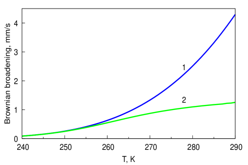
Figure 2: Brownian broadening of the absorption lines vs temperature for the magnetite nanoparticles with diameter $a_{h}=a_{c}=700$ nm in the 60% glycerol-water mixture, calculated in the diffusion approach (1) and Langevin’s one (2)

In order to find now the integral width of $j$th Zeeman line we employ standard formula

$$\Gamma_{\textrm{\scriptsize{int}}}=\frac{2}{\pi\sigma^{(j)}_{a}(\hbar\alpha_{j})}\int_{-\infty}^{\infty}\sigma^{(j)}_{a}(s)ds.$$ (68)

Simple calculation gives

$$\Gamma_{\textrm{\scriptsize{int}}}=e^{-b_{t}}\left[\sum_{n=0}^{\infty}\frac{(-1)^{n}}{n!}\frac{(b_{t})^{n}}{\langle\Gamma_{n}\rangle}\right]^{-1},$$ (69)

where the width $\langle\Gamma_{n}\rangle=\langle\Gamma_{\textrm{\scriptsize{eff}}}\rangle+2n\hbar\beta_{t}$ and the averaged effective width is determined by

$$\langle\Gamma_{\textrm{\scriptsize{eff}}}\rangle=\Gamma_{0}+2\hbar\kappa^{2}D_{t}[1+0.3(a_{c}/a_{h})^{2}]+\Delta\Gamma_{N}.$$ (70)

Significance of Langevin’s approach is illustrated by Fig.2, where the Brownian broadening $\langle\Delta\Gamma_{B}\rangle$ for magnetite MNPs with diameter 700 nm is calculated by Eq. (47) (curve 1) and by Eq. (69) (curve 2). In the last case we put $b_{r}=0$, that is describe the translational Brownian motion by Langevin’s equation and the rotational one by simple diffusion equation. Note that in previous articles K ; B2 the Brownian rotation has not been taken into consideration at all.

VI Discussion

It can be easily shown that the considered relaxations do not influence on the overall probability of the absorption without recoil. Really, since

$$\int_{-\infty}^{\infty}\exp(ist/\hbar)ds=2\pi\hbar\delta(t)$$ (71)

and $G_{B}({\bm{\kappa}},0)G_{N}(0)=1$ one gets

$$\int_{-\infty}^{\infty}\sigma_{a}(s)ds=\frac{\pi}{2}\sigma_{0}\Gamma_{a}e^{-2W}.$$ (72)

Thus, the square of the Mössbauer spectrum keeps constant value.

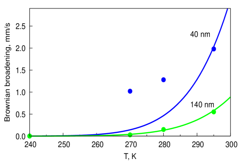
Figure 3: Brownian broadening of the absorption lines vs temperature for the magnetite nanoparticles with diameters 40 nm and 140 nm dissolved in 96% glycerol-water mixture. The experiment Chuev1 is presented by circles, our calculations by solid curves.

We have derived the expression (31) for the absorption cross section $\sigma_{a}(s)$ of Mössbauer radiation by MNPs suspended in a liquid. It will coincide with the result of Blume and Tion Blume , if in the effective width $\Gamma_{\textrm{\scriptsize{eff}}}$ we omit a contribution $\Delta\Gamma_{B}$ of the Brownian motion. But the cross section, averaged over uniform distribution of the nuclei ⁵⁷Fe over the particle, takes a combersome form. The situation significantly simplifies if we replace averaging of $\sigma_{a}(s)$ by the averaging only of $\Delta\Gamma_{B}$. As it is seen in Fig.1, this procedure provides very good result.

We compared our calculations with the experimental data Cher of Cherepanov et al. (see Fig.3). From the Mössbauer spectra of ferrofluids they subtracted the spectra of dried samples. It enabled them to extract the contribution only of Brownian motion into the broadening of the spectral lines. The calculated dependence of the Brownian broadening $\Delta\Gamma_{B}$ on the temperature is presented in Fig.3 by solid lines and the experimental data by circles. The calculations very well agree with the experiment for large particles having diameter 140 nm, and at the same time they terribly deviate for small ones with the dimensions 40 nm. This deviation contradicts to the fact that the viscosity of liquid exponentially decreases with growing temperature, and as a consequence this should ensure for small MNPs the same behavior of $\Delta\Gamma_{B}$ as for large MNPs.

The next part of the paper will be addressed to Mössbauer spectra in ferrofluids subjected to external magnetic fields.

References

- (1) R. E. Rosensweig, Ferrohydrodynamics, Cambridge Univ. Press, Cambridge, London (1985); republished by Dover.Publ.Inc., New York (1997).
- (2) Magnetic Fluids and Applications Handbook , edit. by B. Berkovski and V. Bashtovoy, (Begell House, Wallingford (1996)).
- (3) C. Scherer and A. M. Figueiredo Neto, Brazil. J. Phys. 35, 718 (2005).
- (4) D. H. Wang and W. H. Liao, Smart Mater. Struct. 20, 023001 (2011).
- (5) K. Ray and R. Moskowitz, J. Magn. Magn. Mater. 85, 233 (1990).
- (6) K. Ray, R. Moskowitz, and R. Casciari, J. Magn. Magn. Mater. 149, 174 (1995).
- (7) R. Pérez-Castillejos, J. A. Plaza, J. Esteve, P. Losantos, M. C. Acero, C. Cane, and F. Serra-Mestres, Sens. Actuators A 84, 176 (2000).
- (8) E. H. Kim, H. S. Lee, B. K. Kwak, and B. K. Kim, J. Magn. Magn. Mater. 289, 328 (2005).
- (9) V. V. Mody, A. Singh, and B. Wesley, Eur. J. Nanomed. 5, 11 (2013).
- (10) K. M. Krishnan, IEEE Trans. Magn. 46, 2523 (2010).
- (11) B. Gleich and J. Weizenecker, Nature 435, 1214 (2005).
- (12) R. M. Ferguson, K. R. Minard, A. P. Khandhar and K. M. Krishnan, Med. Phys. 38, 1619 (2011).
- (13) R. J. Deissler, Yong Wu, and M. A. Martens, Med. Phys. 41, 012301 (2014).
- (14) Yufen Xiao and Jianzhong Du, J. Mater. Chem. B 8, 354 (2020).
- (15) H. T. Kim Duong, A. Abdibastami, L. Gloag, L. Barrera, J. J. Gooding, and R. D. Tilley, Nanoscale 14, 13890 (2022).
- (16) L. Néel, Ann. Geophys. 5, 99 (1949).
- (17) J. Landers, S. Salamon, H. Remmer, F.Ludwig, H.Wende, Nano Lett. 16, 1150 (2016).
- (18) P. P. Craig and N. Sutin, Phys. Rev. Let., 11, 460 (1963).
- (19) D. St. P. Bunbury, J. A. Elliott, H. E. Hall, and J. M. Williams, Phys. Let. 6, 34 (1963).
- (20) V. I. Lisichenko, Ukr. J. Phys. 9, 1376 (1964).
- (21) V. N. Dubinin, et al., Ukr. J. Phys 11, 619 (1966).
- (22) T. Bonchev, P. Aidemirski, I. Mandzhukov, N. Nedyalkova, B. Skorchev, and A. Strigachev, Sov. Phys. JETP 23, 42 (1966).
- (23) K. P. Singh and J. G. Mullen, Phys. Rev. A 6, 2354 (1972).
- (24) V. N. Dubinin, Ukr. J. Phys. 13, 1547 (1968).
- (25) C. L. Kordyuk, V. I. Lisichenko, 0. L. Orlov, N. N. Polovina, and A. N. Smoilovskii, Sov. Phys. JETP 25, 400 (1967).
- (26) V. G. Bhide, R. Sundaram, H. C. Bhasin, and T. Bonchev, Phys. Rev. 3, 673 ((1971).
- (27) K. S. Singwi and A. Sjölander, Phys. Rev. 120, 1093 (1960).
- (28) A. V. Zatovskiǐ, Sov. Phys. JETP 32, 274 (1971).
- (29) A. Ya. Dzyublik, Ukr. J. Phys. 18, 1454 (1973).
- (30) A. Ya. Dzyublik, Sov. Phys. JETP 40, 763 (1975).
- (31) A. M. Afanas’ev, P. V. Hendriksen, and S. Mørup, Hyperf. Inter. 88, 35 (1994).
- (32) A. Ya. Dzyublik, Ukr. J. Phys. 23, 881 (1978).
- (33) Joachim Landers, Soma Salamon, Hilke Remmer, Frank Ludwig, and Heiko Wende, ACS Appl. Mater. Interfaces 11, 3160 (2019).
- (34) M. A. Chuev, V. M. Cherepanov, M. A. Polikarpov, R. R. Gabbasov, and A. Yu. Yurenya, JETP Lett. 108, 59 (2018).
- (35) R. Gabbasov, A. Yurenya, A. Nikitin, V. Cherepanov, M. Polikarpov, M. Chuev, A. Majouga, and V. Panchenko, J. Magn. Magn. Mater. 475, 146 (2019).
- (36) V. M. Cherepanov, et al., Crystal. Rep. 65, 398 (2020).
- (37) M. Blume, J. A. Tjon, Phys. Rev. 165, 446 (1968).
- (38) S. Chandrasekhar, Rev. Mod. Phys. 15, 1 (1943).
- (39) A. Einstein, Ann. Phys. 19, 371 (1906).
- (40) M. A. Leontovich, Introduction to Thermodynamics. Statistical Physics (High School, Moscow, 1983) (in Russian).
- (41) L.D.Landau, E.M.Lifshitz, Mechanics 3d Edition (Elsevier Ltd., Oxford, 1976).
- (42) G. Kirchhoff, Vorlesungen über Mechanik (B.G.Teubner, Leipzig, 1897).