The Anytime Convergence of Stochastic Gradient Descent with Momentum: From a Continuous-Time Perspective

Abstract

In this paper, we study the stochastic optimization problem from a continuous-time perspective. We propose a stochastic first-order algorithm, called Stochastic Gradient Descent with Momentum (SGDM), and show that the trajectory of SGDM, despite its stochastic nature, converges to a deterministic second-order Ordinary Differential Equation (ODE) in $L_{2}$-norm, as the stepsize goes to zero. The connection between the ODE and the algorithm results in delightful patterns in the discrete-time convergence analysis. More specifically, we develop convergence results for the ODE through a Lyapunov function, and translate the whole argument to the discrete-time case. This approach yields a novel anytime convergence guarantee for stochastic gradient methods. Precisely, we prove that, for any $\beta$, there exists $k_{0}$ such that the sequence $\{x_{k}\}$ governed by running SGDM on a smooth convex function $f$ satisfies

$$\mathbb{P}\left(\mathop{\bigcap}\limits_{k=k_{0}}^{\infty}\bigg{\{}f(x_{k})-f^{*}\leq\frac{C\log k\log(2/\beta)}{\sqrt{k}}\bigg{\}}\right)\geq 1-\beta,$$

where $f^{*}=\min_{x\in\mathbb{R}^{n}}f(x)$. Our contribution is significant in that it better captures the convergence behavior across the entire trajectory of the algorithm, rather than at a single iterate.

1 Introduction

Stochastic gradient methods are widely used in various fields such as machine learning (e.g., Johnson and Zhang,, 2013; Loizou and Richtárik,, 2017), statistics (e.g., Robbins and Monro,, 1951), and more. These algorithms, including Stochastic Gradient Descent (SGD) and its variants, have been successful in practice. Many research works have focused on establishing convergence guarantees for SGD (Nemirovski et al.,, 2009; Shamir and Zhang,, 2013; Harvey et al.,, 2019) and its variants (Lan,, 2012; Ghadimi and Lan,, 2013; Gitman et al.,, 2019; Li and Orabona,, 2019; Gorbunov et al.,, 2020; Liu et al.,, 2020), aiming to ensure their effectiveness and reliability.

Also, the relationship between continuous-time dynamics and discrete-time algorithms has been extensively studied in mathematics and related fields (Helmke and Moore,, 1996). Recently, there is a resurgence of interest in understanding the continuous-time interpretation of discrete-time algorithms, inspired by the ODE modeling of Nesterov’s accelerated gradient method (Su et al.,, 2014). This new perspective leads to valuable insights in the analysis (Wibisono et al.,, 2016; Shi et al.,, 2021) and design (Krichene et al.,, 2015; Zhang et al.,, 2018; Shi et al.,, 2019; Zhang et al.,, 2021) of deterministic optimization algorithms.

The correspondence between continuous-time dynamics and discrete-time algorithms has also been explored in the context of stochastic optimization (Mandt et al.,, 2016; Li et al.,, 2017; He et al.,, 2018; Orvieto and Lucchi,, 2019; Cheng et al.,, 2020; Shi,, 2021; Difonzo et al.,, 2022). Previous work by Cheng et al., (2020) investigated numeric SDEs in machine learning applications, motivated by stochastic gradient algorithms. However, the continuous-time limit of some stochastic optimization methods, including the algorithm proposed in this paper, exhibits different behavior. Specifically, the stochasticity disappears as the stepsize goes to zero. In contrast, previous studies on Langevin dynamics have focused on analyzing the Euler scheme for SDEs. More related works are discussed in Appendix A.

In this paper, we consider the optimization problem $\min_{x\in\mathbb{R}^{n}}f(x)$, in an environment where $f$ is accessible only through a stochastic gradient oracle. That is, if we query the oracle at $x$, it returns a stochastic version $g(x,\xi)$ of the gradient $\nabla f(x)$, and the randomness in different oracle calls are independent. We use $x^{*}$ to denote an optimal solution of this problem, and $f^{*}=f(x^{*})=\min_{x\in\mathbb{R}^{n}}f(x)$ is the minimal function value. Our main focus is on studying the Stochastic Gradient Descent with Momentum (SGDM) method given by

$$\begin{split}&x_{k}-x_{k-1}=\eta v_{k-1},\\ &v_{k}-v_{k-1}=-\frac{2}{k}v_{k}-\frac{2}{k}\cdot\frac{1}{\sqrt{k\eta}}g(x_{k},\xi_{k}),\end{split}$$ (1)

where $\eta$ is the stepsize. From a continuous-time perspective, we rigorously prove that as $\eta$ tends to zero, the sequence $\{x_{k}\}$ generated by SGDM converges to the trajectory of the second-order ODE

$$\ddot{X}(t)+\frac{2}{t}\dot{X}(t)+\frac{2}{t^{3/2}}\nabla f(X(t))=0$$ (2)

in $L_{2}$-norm. This continuous-time correspondence provides insights into the discrete-time analysis. More specifically, we establish the convergence guarantees of the ODE (2) using a Lyapunov analysis and then translate our entire argument to the discrete-time case. By taking advantage of this approach, our results contribute to the existing literature on stochastic gradient methods, particularly in terms of the anytime high probability convergence guarantee of SGDM under mild conditions.

1.1 The Anytime High Probability Convergence and Our Contributions

For theoretical analysis of stochastic optimization algorithms, an important topic is to develop convergence guarantees that hold with high probability (Nemirovski et al.,, 2009; Lan,, 2012; Nazin et al.,, 2019; Gorbunov et al.,, 2020; Liu et al.,, 2023). This is partially because the high probability analysis better reflects the performance of a single run of the algorithm. For a given probability $1-\beta$, the existing results always take the form:

$$\text{\emph{For each $k\in\mathbb{N}$}},\;\mathbb{P}\left(f(x_{k})-f^{*}\leq\widetilde{U}(k,\beta)\right)\geq 1-\beta,$$ (3)

where $\widetilde{U}(k,\beta)$ represents an upper bound depending on $k$ and $\beta$. However, the guarantee (3) is insufficient if a practitioner wants to capture the behavior of the whole trajectory of the algorithm, or requires the upper bound to remain valid with high probability at any data-dependent stopping time (Waudby-Smith and Ramdas,, 2020; Howard et al.,, 2021). Instead, the following condition must be met:

$$\mathbb{P}\left(\forall k,\;f(x_{k})-f^{*}\leq U(k,\beta)\right)\geq 1-\beta.$$ (4)

We shall refer to results of the form (4) as anytime high probability guarantees, and they are of essential importance when the behavior of the entire trajectory, rather than a single iterate, is used in decision-making, as is the case with hyperparameter optimization (Jamieson and Talwalkar,, 2016; Li et al.,, 2018). Furthermore, this concept is closely related to the confidence sequence, which has been widely investigated in sequential statistics (Lai,, 1976; Sinha and Sarkar,, 1984) and applied to online learning (Jamieson et al.,, 2014; Kaufmann and Koolen,, 2021; Orabona and Jun,, 2023). However, to the best of our knowledge, anytime convergence guarantees have not been studied in the stochastic optimization literature. One may derive (4) from (3) by taking union bounds, but this will cause a worse upper bound $U(k,\beta)$, in terms of its dependence on $k$. Therefore, it is natural to ask:

Is it possible to establish an anytime guarantee (4), with the upper bound no worse than that of (3)?

In this paper, we leverage a new continuous-time perspective to close this gap. We provide the first anytime high probability result of the form (4) for stochastic gradient methods, as well as give an affirmative answer to the above question. Our main contributions are as follows.

1. We are the first to rigorously show that the continuous-time limit of a momentumized stochastic gradient method is a deterministic second-order ODE. Furthermore, we use our result of this ODE as a guidance for the algorithm analysis. As we will discuss later, this approach better reveals the intrinsic dynamic property of SGDM, leading to the new convergence results.

2. We establish the first anytime high probability convergence guarantee for stochastic gradient methods. We prove that, for any $\beta$, there exists $k_{0}$ such that the sequence $\{x_{k}\}$ governed by running SGDM on a smooth convex function $f$ satisfies

   $$\mathbb{P}\left(\forall k\geq k_{0},\;f(x_{k})-f^{*}\leq\frac{C_{0}\log k_{0}\cdot\log k\log\frac{2}{\beta}}{\sqrt{k}}\right)\geq 1-\beta,$$ (5)

   where $C_{0}$ is a constant. As far as we know, no prior research on stochastic gradient methods has studied the probability that the convergence bound holds simultaneously over iterates. In this work, we propose a novel procedure for proving this anytime high probability convergence without losing any factors in $k$, compared to its single-iterate counterpart. More specifically, we first demonstrate that SGDM converges on almost every sample path through a supermartingale convergence argument, and then fuse this result with our high probability analysis. We utilize the discrete-time Lyapunov function, introduced from our continuous-time analysis, as the pivotal element that unites these two methodologies, culminating in the establishment of the anytime high probability convergence bound.

3. We also provide a new technique in the high probability analysis. We prove that the martingale difference sequence arising in the argument can be bounded by our discrete-time Lyapunov function. As a consequence, the anytime convergence guarantee (5) does not rely on any projection, or the assumption of bounded gradients or stochastic gradients. In addition, our result is for the last iterate, and does not need any averaging step.

4. For smooth convex objective functions, we show that with probability $1$ there exists a sub-sequence $\{x_{k_{l}}\}$ of $\{x_{k}\}$ generated by SGDM satisfies $f(x_{k_{l}})-f^{*}=o\left(\frac{1}{\sqrt{k_{l}}\log\log k_{l}}\right)$. This rate is new to the best of our knowledge.

Figure 1: The framework of our theoretical analysis.

This paper is organized as follows. In section 2, we prove that the continuous-time limit of SGDM is the ODE (2), and then construct a Lyapunov function to give the convergence result of (2). In Section 3, we translate the Lyapunov argument to the discrete case and prove the convergence of SGDM in expectation. In addition, we demonstrate the almost sure convergence by the supermartingale convergence theorem. Moving on to Section 4, we provide the convergence result of SGDM with high probability, without requiring any projection or bounded gradient assumption. We accomplish this by utilizing our Lyapunov function. Finally, we make use of all the above results and establish the anytime high probability convergence guarantee of SGDM. We present the experimental results in Section 5, which confirm our theoretical findings. Figure 1 illustrates the entire framework of our theoretical analysis.

1.2 Existing High Probability Results

There have been substantial advancements in establishing high probability guarantees for stochastic gradient methods. Nemirovski et al., (2009) established convergence guarantees for a robust stochastic approximation approach. Lan, (2012) proposed an accelerated method that is universally optimal for solving non-smooth, smooth, and stochastic problems. Ghadimi and Lan, (2013) developed a two-phase method to improve the large deviation properties. Nazin et al., (2019), Madden et al., (2020), Gorbunov et al., (2020), Cutkosky and Mehta, (2021), and Li and Liu, (2022) proposed high probability convergence results without the light-tailed assumption. Li and Orabona, (2020) and Kavis et al., (2021) studied stochastic gradient methods with adaptive stepsize. Liu et al., (2023) provided a new concentration argument to improve the high probability analysis. The last-iterate high probability convergence results for SGD is studied by Harvey et al., (2019). Jain et al., (2021) introduced a stepsize sequence to obtain the optimal last-iterate convergence bound. Liu and Zhou, (2023) also presented a unified way for enhancing the last-iterate convergence analysis of stochastic gradient methods. Yet all of the existing works provide high probability results that hold for individual $k$, and none of them study the anytime convergence, or more specifically, the probability that the convergence guarantee holds simultaneously over all values of $k$. A survey of more related works on stochastic optimization is provided in Appendix A, including existing in expectation convergence results.

2 Continuous-Time Analysis

In this section, we show that the continuous-time limit of SGDM is the ODE (2), and construct a Lyapunov function to derive the convergence result of (2). Our analysis relies on the following assumption on the objective function $f$.

Assumption 1.

$f$ is convex and $L$-smooth, that is, $\|\nabla f(x)-\nabla f(y)\|\leq L\|x-y\|$ for any $x,y\in\mathbb{R}^{n}$. There exists $x^{*}=\arg\min_{x\in\mathbb{R}^{n}}f(x)$.

2.1 Derivation of the ODE Model

We rewrite (2) as the following system

$$\left\{\begin{aligned} &\frac{\mathrm{d}X}{\mathrm{d}t}=V,\\ &\frac{\mathrm{d}V}{\mathrm{d}t}=-\frac{2}{t}V-\frac{2}{{t}^{\frac{3}{2}}}\nabla f(X).\end{aligned}\right.$$ (6)

Theorem 1 shows that the stochastic sequence $\{x_{k}\}$ generated by SGDM converges to the trajectory of the deterministic ODE system (6) as the stepsize goes to zero. For our purpose, we consider the ODE system (6) starting at an arbitrary $T_{0}>0$.

Theorem 1.

Assume that $f$ is $L$-smooth. Let $(X(t),V(t))$ be the solution of the ODE system (6), and $\{(x_{k},v_{k})\}$ be generated by SGDM (1) with the stochastic gradients satisfying $g(x_{k},\xi_{k})=\nabla f(x_{k})+\xi_{k}$ for each $k$, where $\xi_{k}\overset{iid}{\sim}\mathcal{N}(0,I_{n})$. If $X(T_{0})=x_{T_{0}/\eta}$ and $V(T_{0})=v_{T_{0}/\eta}$ for $T_{0}>0$, then

$$\lim_{\eta\to 0}\mathbb{E}\left[\|x_{T/\eta}-X(T)\|^{2}\right]=0$$

holds for any $T>T_{0}$.

The proof of Theorem 1 relies on constructing auxiliary SDEs with diminishing stochastic term, and stochastic calculus techniques calibrated to our setting. Before presenting the detailed proof, we shall give an informal derivation of the ODE (2) and (6).

We rewrite SGDM scheme (1) as

$$\left\{\begin{aligned} &x_{k}-x_{k-1}=\eta v_{k-1},\\ &v_{k}-v_{k-1}=-\frac{2}{k\eta}v_{k}\eta-\frac{2}{(k\eta)^{\frac{3}{2}}}\nabla f(x_{k})\eta-\frac{2}{(k\eta)^{\frac{3}{2}}}(\sqrt{\eta}\xi_{k})\sqrt{\eta}.\end{aligned}\right.$$ (7)

Let $W$ be a standard Brownian motion. Then we let $\eta$ in (7) go to zero and replace $x_{k}-x_{k-1}$, $v_{k}-v_{k-1}$, $k\eta$, $\eta$ and $\sqrt{\eta}\xi$ by $\mathrm{d}X$, $\mathrm{d}V$, $t$, $\mathrm{d}t$ and $dW$, respectively. The discrete scheme (7) becomes

$$\left\{\begin{aligned} &\mathrm{d}X=V\mathrm{d}t,\\ &\mathrm{d}V=-\frac{2}{t}V\mathrm{d}t-\frac{2}{{t}^{\frac{3}{2}}}\nabla f(X)\mathrm{d}t-\frac{2}{t^{\frac{3}{2}}}\sqrt{\mathrm{d}t}\mathrm{d}W.\end{aligned}\right.$$

Since $\sqrt{\mathrm{d}t}\mathrm{d}W$ is a higher order term, we omit it and obtain (6), which leads to the ODE (2) by subscribing the first line to the second line.

Proof of Theorem 1.

For any fixed $\eta>0$, we write $t_{k}=k\eta$ and consider an auxiliary SDE system $\bigl{(}\widetilde{X}(t),\widetilde{V}(t)\bigr{)}$ on $[T_{0},T]$ with initialization $\widetilde{X}(T_{0})=x_{T_{0}/\eta}$ and $\widetilde{V}(T_{0})=v_{T_{0}/\eta}$, which is defined as

$$\left\{\begin{aligned} &\mathrm{d}\widetilde{X}(t)=\widetilde{V}(t_{k})\mathrm{d}t,\\ &\mathrm{d}\widetilde{V}(t)=-\frac{2}{t_{k}}\widetilde{V}(t_{k})\mathrm{d}t-\frac{2}{t_{k}^{\frac{3}{2}}}\nabla f\left(\widetilde{X}(t_{k})\right)\mathrm{d}t-\frac{2}{t_{k}^{\frac{3}{2}}}\sqrt{\eta}dW(t),\end{aligned}\right.$$ (8)

for $t\in[t_{k},t_{k+1})$. Integrating sequentially on each interval $[t_{k},t_{k+1})$ shows that $\bigl{(}\widetilde{X}(t_{k}),\widetilde{V}(t_{k})\bigr{)}$ and $(x_{k},v_{k})$ are identically distributed for each $T_{0}\leq t_{k}\leq T$. For convenience, we denote

$$\widetilde{Y}(t)=\begin{pmatrix}\widetilde{X}(t)\\ \widetilde{V}(t)\end{pmatrix}\quad\text{and}\quad Y(t)=\begin{pmatrix}X(t)\\ V(t)\end{pmatrix},$$

where $X(t)$ and $V(t)$ are defined in the ODE system (6), and thus $\mathbb{E}\Bigl{[}\bigl{\|}x_{T/\eta}-X(T)\bigr{\|}^{2}\Bigr{]}=\mathbb{E}\Bigl{[}\bigl{\|}\widetilde{X}(T)-X(T)\bigr{\|}^{2}\Bigl{]}\leq\mathbb{E}\Bigl{[}\bigl{\|}\widetilde{Y}(T)-Y(T)\bigr{\|}^{2}\Bigr{]}$. The following lemma shows that $\{\widetilde{Y}(t_{k})\}$ are uniformly bounded in $L_{2}$-norm.

Lemma 1.

Let $[T_{0},T]$ be a fixed horizon. There exists a constant $C_{1}$ such that for any $\eta>0$,

$$\max_{\frac{T_{0}}{\eta}\leq k\leq\frac{T}{\eta}}\mathbb{E}\Bigl{[}\bigl{\|}\widetilde{Y}(t_{k})\bigr{\|}^{2}\Bigr{]}\leq C_{1},$$ (9)

where $t_{k}=k\eta$. Furthermore, there exists a constant $C_{2}$ such that for any $\eta>0$ and any $T_{0}\leq t_{k}\leq t\leq t_{k+1}\leq T$,

$$\mathbb{E}\Bigl{[}\bigl{\|}\widetilde{Y}(t)-\widetilde{Y}(t_{k})\bigr{\|}^{2}\Bigr{]}\leq C_{2}\eta^{2}.$$ (10)

Proof.

The definition (8) gives that

$$\widetilde{Y}(t)-\widetilde{Y}(t_{k})=\begin{pmatrix}\widetilde{V}(t_{k})\\ -\frac{2}{t_{k}}\widetilde{V}(t_{k})-\frac{2}{t_{k}^{\frac{3}{2}}}\nabla f(\widetilde{X}(t_{k}))\end{pmatrix}\cdot(t-t_{k})+\begin{pmatrix}0\\ -\frac{2}{t_{k}^{\frac{3}{2}}}\sqrt{\eta}(W(t)-W(t_{k}))\end{pmatrix},$$

for any $t_{k}\leq t\leq t_{k+1}$. The $L$-smoothness gives that

$$\|\nabla f(x)\|=\|\nabla f(x)-\nabla f(x^{*})\|\leq L\cdot\|x-x^{*}\|\leq L\|x\|+L\|x^{*}\|.$$ (11)

Therefore, we have

$$\bigl{\|}\widetilde{Y}(t)-\widetilde{Y}(t_{k})\bigr{\|}^{2}\leq 2\left(\bigl{\|}\widetilde{V}(t_{k})\bigr{\|}^{2}+\frac{8}{t_{k}^{2}}\bigl{\|}\widetilde{V}(t_{k})\bigr{\|}^{2}+\frac{16L^{2}}{t_{k}^{3}}\left(\bigl{\|}\widetilde{X}(t_{k})\bigr{\|}^{2}+\|x^{*}\|^{2}\right)\right)(t-t_{k})^{2}$$

$$+\frac{8}{t_{k}^{3}}\eta(W(t)-W(t_{k}))^{2},$$

and thus there exists a constant $C_{3}$, depending on $T_{0}$, $\|x^{*}\|$ and $L$, such that

$$\bigl{\|}\widetilde{Y}(t)-\widetilde{Y}(t_{k})\bigr{\|}^{2}\leq C_{3}\left(\bigl{\|}\widetilde{Y}(t_{k})\bigr{\|}^{2}+1\right)(t-t_{k})^{2}+C_{3}\eta(W(t)-W(t_{k}))^{2}.$$

Since $t\leq t_{k+1}=t_{k}+\eta$, taking expectation on both sides yields that

$$\mathbb{E}\Bigl{[}\bigl{\|}\widetilde{Y}(t)-\widetilde{Y}(t_{k})\bigr{\|}^{2}\Bigr{]}\leq 2C_{3}\eta^{2}\left(\mathbb{E}\Bigl{[}\bigl{\|}\widetilde{Y}(t_{k})\bigr{\|}^{2}\Bigr{]}+1\right).$$ (12)

Specifically, by letting $t=t_{k+1}$ we have

$$\mathbb{E}\Bigl{[}\bigl{\|}\widetilde{Y}(t_{k+1})-\widetilde{Y}(t_{k})\bigr{\|}^{2}\Bigr{]}\leq 2C_{3}\eta^{2}\left(\mathbb{E}\Bigl{[}\bigl{\|}\widetilde{Y}(t_{k})\bigr{\|}^{2}\Bigr{]}+1\right).$$

We denote

$$a_{n}=\max_{\frac{T_{0}}{\eta}\leq k\leq\frac{T_{0}}{\eta}+n}\left(\mathbb{E}\Bigl{[}\bigl{\|}\widetilde{Y}(t_{k})\bigr{\|}^{2}\Bigr{]}\right)^{\frac{1}{2}},$$

and we have

$$a_{n+1}\leq a_{n}+\left(\mathbb{E}\Bigl{[}\bigl{\|}\widetilde{Y}(t_{k+1})-\widetilde{Y}(t_{k})\bigr{\|}^{2}\Bigr{]}\right)^{\frac{1}{2}} \leq a_{n}+\sqrt{2C_{3}}\eta\left(\mathbb{E}\Bigl{[}\bigl{\|}\widetilde{Y}(t_{k})\bigr{\|}^{2}\Bigr{]}+1\right)^{\frac{1}{2}}$$

$$\leq(1+\sqrt{2C_{3}}\eta)a_{n}+\sqrt{2C_{3}}\eta.$$

Therefore, for $N=\frac{T-T_{0}}{\eta}$, we have

$$a_{N} \leq(1+\sqrt{2C_{3}}\eta)^{N}a_{0}+\sqrt{2C_{3}}\eta\sum_{k=0}^{N-1}(1+\sqrt{2C_{3}}\eta)^{k}$$

$$\leq\left(1+\frac{\sqrt{2C_{3}}(T-T_{0})}{N}\right)^{N}a_{0}+\frac{\sqrt{2C_{3}}(T-T_{0})}{N}\cdot N\left(1+\frac{\sqrt{2C_{3}}(T-T_{0})}{N}\right)^{N}$$

$$\leq e^{\sqrt{2C_{3}}(T-T_{0})}\left(\mathbb{E}\Bigl{[}\bigl{\|}\widetilde{Y}(T_{0})\bigr{\|}^{2}\Bigr{]}\right)^{\frac{1}{2}}+\sqrt{2C_{3}}(T-T_{0})e^{\sqrt{2C_{3}}(T-T_{0})}.$$

Thus, we finish the proof of (9) by letting

$$C_{1}=\left(e^{\sqrt{2C_{3}}(T-T_{0})}\left(\mathbb{E}\Bigl{[}\bigl{\|}\widetilde{Y}(T_{0})\bigr{\|}^{2}\Bigr{]}\right)^{\frac{1}{2}}+\sqrt{2C_{3}}(T-T_{0})e^{\sqrt{2C_{3}}(T-T_{0})}\right)^{2}.$$

For the second part, we substitute (9) to (12) to conclude that

$$\mathbb{E}\Bigl{[}\bigl{\|}\widetilde{Y}(t)-\widetilde{Y}(t_{k})\bigr{\|}^{2}\Bigr{]}\leq 2C_{3}\eta^{2}\left(C_{1}+1\right)=C_{2}\eta^{2},$$

where $C_{2}=2C_{3}(C_{1}+1)$. ∎

In the remaining proof, we will upper bound

$$\mathrm{d}\mathbb{E}\Bigl{[}\bigl{\|}\widetilde{Y}(t)-Y(t)\bigr{\|}^{2}\Bigr{]}=\mathrm{d}\mathbb{E}\Bigl{[}\bigl{\|}\widetilde{X}(t)-X(t)\bigr{\|}^{2}\Bigr{]}+\mathrm{d}\mathbb{E}\Bigl{[}\bigl{\|}\widetilde{V}(t)-V(t)\bigr{\|}^{2}\Bigr{]},$$ (13)

and then apply the Grönwall’s inequality to $\mathbb{E}\Bigl{[}\bigl{\|}\widetilde{Y}(t)-Y(t)\bigr{\|}^{2}\Bigr{]}$, which yields the convergence result of Theorem 1.

For the first term on the RHS of (13), the Itô’s formula yields that

$$\mathrm{d}\bigl{\|}\widetilde{X}(t)-X(t)\bigr{\|}^{2} =2\bigl{(}\widetilde{X}(t)-X(t)\bigr{)}^{\mathsf{T}}\mathrm{d}\bigl{(}\widetilde{X}(t)-X(t)\bigr{)}+\mathrm{d}\mathop{\mathrm{tr}}\bigl{[}\widetilde{X}-X\bigr{]}(t),$$

where $\bigl{[}\widetilde{X}-X\bigr{]}$ is the quadratic variation process of $\widetilde{X}-X$. The definitions (6) and (8) yields that $\mathrm{d}\bigl{(}\widetilde{X}(t)-X(t)\bigr{)}=\bigl{(}\widetilde{V}(t_{k})-V(t)\bigr{)}\mathrm{d}t$. Since $\widetilde{X}-X$ is of finite variation, we have $\bigl{[}\widetilde{X}-X\bigr{]}(t)=0$. We thus derive

$$\begin{split}\mathrm{d}\bigl{\|}\widetilde{X}(t)-X(t)\bigr{\|}^{2}&=2\bigl{(}\widetilde{X}(t)-X(t)\bigr{)}^{\mathsf{T}}\bigl{(}\widetilde{V}(t_{k})-\widetilde{V}(t)+\widetilde{V}(t)-V(t)\bigr{)}\mathrm{d}t\\ &=2\bigl{(}\widetilde{X}(t)-X(t)\bigr{)}^{\mathsf{T}}\bigl{(}\widetilde{V}(t_{k})-\widetilde{V}(t)\bigr{)}\mathrm{d}t+2\bigl{(}\widetilde{X}(t)-X(t)\bigr{)}^{\mathsf{T}}\bigl{(}\widetilde{V}(t)-V(t)\bigr{)}\mathrm{d}t\\ &\leq\bigl{\|}\widetilde{X}(t)-X(t)\bigr{\|}^{2}\mathrm{d}t+\bigl{\|}\widetilde{V}(t_{k})-\widetilde{V}(t)\bigr{\|}^{2}\mathrm{d}t+\bigl{\|}\widetilde{X}(t)-X(t)\bigr{\|}^{2}\mathrm{d}t+\bigl{\|}\widetilde{V}(t)-V(t)\bigr{\|}^{2}\mathrm{d}t.\end{split}$$ (14)

From (10) we have $\mathbb{E}\left[\bigl{\|}\widetilde{V}(t_{k})-\widetilde{V}(t)\bigr{\|}^{2}\right]\leq C_{2}\eta^{2}$. Therefore, taking expectation on both sides of (14) gives that

$$\mathrm{d}\mathbb{E}\left[\bigl{\|}\widetilde{X}(t)-X(t)\bigr{\|}^{2}\right]\leq 3\mathbb{E}\left[\bigl{\|}\widetilde{Y}(t)-Y(t)\bigr{\|}^{2}\right]\mathrm{d}t+C_{2}\eta^{2}\mathrm{d}t.$$ (15)

For the second term on the RHS of (13), the Itô’s formula yields that

$$\mathrm{d}\bigl{\|}\widetilde{V}(t)-V(t)\bigr{\|}^{2} =2\left(\widetilde{V}(t)-V(t)\right)^{\mathsf{T}}\mathrm{d}\left(\widetilde{V}(t)-V(t)\right)+\mathrm{d}\mathop{\mathrm{tr}}\bigl{[}\widetilde{V}-V\bigr{]}(t).$$ (16)

The definition (6) and (8) yields that

$$\mathrm{d}\left(\widetilde{V}(t)-V(t)\right)=-\left(\frac{2}{t_{k}}\widetilde{V}(t_{k})-\frac{2}{t}V(t)\right)\mathrm{d}t-\left(\frac{2}{t_{k}^{\frac{3}{2}}}\nabla f(\widetilde{X}(t_{k}))-\frac{2}{t^{\frac{3}{2}}}\nabla f(X(t))\right)\mathrm{d}t-\frac{2}{t_{k}^{\frac{3}{2}}}\sqrt{\eta}\mathrm{d}W(t).$$

Then the definition of quadratic variation gives

$$\mathrm{d}\mathop{\mathrm{tr}}\bigl{[}\widetilde{V}-V\bigr{]}(t)=\frac{4n}{t_{k}^{3}}\eta\mathrm{d}t\leq\frac{4n}{T_{0}^{3}}\eta\mathrm{d}t.$$ (17)

We also have

$$\begin{split}2\left(\widetilde{V}(t)-V(t)\right)^{\mathsf{T}}\mathrm{d}\left(\widetilde{V}(t)-V(t)\right)=&\underbrace{-\left(\widetilde{V}(t)-V(t)\right)^{\mathsf{T}}\left(\frac{4}{t_{k}}\widetilde{V}(t_{k})-\frac{4}{t}V(t)\right)\mathrm{d}t}_{\text{\char 172}}\\ &\underbrace{-\left(\widetilde{V}(t)-V(t)\right)^{\mathsf{T}}\left(\frac{4}{t_{k}^{\frac{3}{2}}}\nabla f(\widetilde{X}(t_{k}))-\frac{4}{t^{\frac{3}{2}}}\nabla f(X(t))\right)\mathrm{d}t}_{\text{\char 173}}\\ &\underbrace{-\left(\widetilde{V}(t)-V(t)\right)^{\mathsf{T}}\cdot\frac{4}{t_{k}^{\frac{3}{2}}}\sqrt{\eta}\mathrm{d}W(t)}_{\text{\char 174}}.\end{split}$$ (18)

For ①, we have

$$\begin{split}\text{\char 172}=&-\left(\widetilde{V}(t)-V(t)\right)^{\mathsf{T}}\left(\frac{4}{t_{k}}\widetilde{V}(t_{k})-\frac{4}{t}\widetilde{V}(t)+\frac{4}{t}\widetilde{V}(t)-\frac{4}{t}V(t)\right)\mathrm{d}t\\ =&-\left(\widetilde{V}(t)-V(t)\right)^{\mathsf{T}}\left(\frac{4}{t_{k}}\widetilde{V}(t_{k})-\frac{4}{t}\widetilde{V}(t)\right)\mathrm{d}t-\left(\widetilde{V}(t)-V(t)\right)^{\mathsf{T}}\left(\frac{4}{t}\widetilde{V}(t)-\frac{4}{t}V(t)\right)\mathrm{d}t\\ \leq&\bigl{\|}\widetilde{V}(t)-V(t)\bigr{\|}^{2}\mathrm{d}t+\bigl{\|}\frac{2}{t_{k}}\widetilde{V}(t_{k})-\frac{2}{t}\widetilde{V}(t)\bigr{\|}^{2}\mathrm{d}t+\bigl{\|}\widetilde{V}(t)-V(t)\bigr{\|}^{2}\mathrm{d}t+\frac{4}{T_{0}^{2}}\bigl{\|}\widetilde{V}(t)-V(t)\bigr{\|}^{2}\mathrm{d}t.\end{split}$$ (19)

We note that

$$\left\|\frac{2}{t_{k}}\widetilde{V}(t_{k})-\frac{2}{t}\widetilde{V}(t)\right\|^{2}\mathrm{d}t= \left\|\frac{2}{t_{k}}\widetilde{V}(t_{k})-\frac{2}{t}\widetilde{V}(t_{k})+\frac{2}{t}\widetilde{V}(t_{k})-\frac{2}{t}\widetilde{V}(t)\right\|^{2}\mathrm{d}t$$

$$\leq 2\left(\frac{2\eta}{T_{0}^{2}}\right)^{2}\left\|\widetilde{V}(t_{k})\right\|^{2}\mathrm{d}t+\frac{4}{T_{0}^{2}}\left\|\widetilde{V}(t_{k})-\widetilde{V}(t)\right\|^{2}\mathrm{d}t.$$

Lemma 1 gives that $\mathbb{E}\Bigl{[}\bigl{\|}\widetilde{V}(t_{k})\bigr{\|}^{2}\Bigr{]}\leq C_{1}$ and $\mathbb{E}\Bigl{[}\bigl{\|}\widetilde{V}(t_{k})-\widetilde{V}(t)\bigr{\|}^{2}\Bigr{]}\leq C_{2}\eta^{2}$, so by taking expectation on both sides of the above inequality, we further have

$$\mathbb{E}\left[\left\|\frac{2}{t_{k}}\widetilde{V}(t_{k})-\frac{2}{t}\widetilde{V}(t)\right\|^{2}\right]\mathrm{d}t\leq\left(\frac{8C_{1}}{T_{0}^{4}}+\frac{4C_{2}}{T_{0}^{2}}\right)\eta^{2}\mathrm{d}t.$$ (20)

Therefore, we denote $C_{4}=\frac{8C_{1}}{T_{0}^{4}}+\frac{4C_{2}}{T_{0}^{2}}$, and (19) gives that

$$\mathbb{E}[\text{\char 172}]\leq\left(2+\frac{4}{T_{0}^{2}}\right)\mathbb{E}\Bigl{[}\bigl{\|}\widetilde{Y}(t)-Y(t)\bigr{\|}^{2}\Bigr{]}\mathrm{d}t+C_{4}\eta^{2}\mathrm{d}t.$$ (21)

For ②, we have

$$\begin{split}\text{\char 173}=&-\left(\widetilde{V}(t)-V(t)\right)^{\mathsf{T}}\left(\frac{4}{t_{k}^{\frac{3}{2}}}\nabla f(\widetilde{X}(t_{k}))-\frac{4}{t^{\frac{3}{2}}}\nabla f(\widetilde{X}(t))+\frac{4}{t^{\frac{3}{2}}}\nabla f(\widetilde{X}(t))-\frac{4}{t^{\frac{3}{2}}}\nabla f(X(t))\right)\mathrm{d}t\\ =&-\left(\widetilde{V}(t)-V(t)\right)^{\mathsf{T}}\left(\frac{4}{t_{k}^{\frac{3}{2}}}\nabla f(\widetilde{X}(t_{k}))-\frac{4}{t^{\frac{3}{2}}}\nabla f(\widetilde{X}(t))\right)\mathrm{d}t\\ &-\left(\widetilde{V}(t)-V(t)\right)^{\mathsf{T}}\left(\frac{4}{t^{\frac{3}{2}}}\nabla f(\widetilde{X}(t))-\frac{4}{t^{\frac{3}{2}}}\nabla f(X(t))\right)\mathrm{d}t\\ \leq&\left\|\widetilde{V}(t)-V(t)\right\|^{2}\mathrm{d}t+\left\|\frac{2}{t_{k}^{\frac{3}{2}}}\nabla f(\widetilde{X}(t_{k}))-\frac{2}{t^{\frac{3}{2}}}\nabla f(\widetilde{X}(t))\right\|^{2}\mathrm{d}t\\ &+\left\|\widetilde{V}(t)-V(t)\right\|^{2}\mathrm{d}t+\frac{4L^{2}}{T_{0}^{3}}\left\|\widetilde{X}(t)-X(t)\right\|^{2}\mathrm{d}t.\end{split}$$ (22)

Similar argument to (20) and (11) shows that there exists constant $C_{5}$ such that

$$\mathbb{E}\left[\left\|\frac{2}{t_{k}^{\frac{3}{2}}}\nabla f(\widetilde{X}(t_{k}))-\frac{2}{t^{\frac{3}{2}}}\nabla f(\widetilde{X}(t))\right\|^{2}\right]\mathrm{d}t\leq C_{5}\eta^{2}\mathrm{d}t.$$

Therefore, (22) gives that

$$\mathbb{E}[\text{\char 173}]\leq\left(2+\frac{4L}{T_{0}^{3}}\right)\mathbb{E}\Bigl{[}\bigl{\|}\widetilde{Y}(t)-Y(t)\bigr{\|}^{2}\Bigr{]}\mathrm{d}t+C_{5}\eta^{2}\mathrm{d}t.$$ (23)

Additionally, by Lemma 1 we show ③ is a true martingale, and thus we derive

$$\mathbb{E}[\text{\char 174}]=0.$$ (24)

As a consequence, taking expectation on both sides of (16) and substituting (17), (18), (21), (23), and (24) give that

$$\mathrm{d}\mathbb{E}\Bigl{[}\bigl{\|}\widetilde{V}(t)-V(t)\bigr{\|}^{2}\Bigr{]}\leq\left(4+\frac{4}{T_{0}^{2}}+\frac{4L}{T_{0}^{3}}\right)\mathbb{E}\Bigl{[}\bigl{\|}\widetilde{Y}(t)-Y(t)\bigr{\|}^{2}\Bigr{]}\mathrm{d}t+\left(C_{4}\eta^{2}+C_{5}\eta^{2}+\frac{4n}{T_{0}^{3}}\eta\right)\mathrm{d}t.$$ (25)

Substituting (15) and (25) to (13) yields that

$$\mathrm{d}\mathbb{E}\Bigl{[}\bigl{\|}\widetilde{Y}(t)-Y(t)\bigr{\|}^{2}\Bigr{]}\leq\left(7+\frac{4}{T_{0}^{2}}+\frac{4L}{T_{0}^{3}}\right)\mathbb{E}\Bigl{[}\bigl{\|}\widetilde{Y}(t)-Y(t)\bigr{\|}^{2}\Bigr{]}\mathrm{d}t+\left(C_{2}\eta^{2}+C_{4}\eta^{2}+C_{5}\eta^{2}+\frac{4n}{T_{0}^{3}}\eta\right)\mathrm{d}t.$$

Without loss of generality, we let $\eta<1$. Thus, there exist constants $C_{6}$ and $C_{7}$ such that

$$\mathrm{d}\mathbb{E}\Bigl{[}\bigl{\|}\widetilde{Y}(t)-Y(t)\bigr{\|}^{2}\Bigr{]}\leq C_{6}\mathbb{E}\Bigl{[}\bigl{\|}\widetilde{Y}(t)-Y(t)\bigr{\|}^{2}\Bigr{]}\mathrm{d}t+C_{7}\eta\mathrm{d}t.$$

The Grönwall’s inequality gives that

$$\mathbb{E}\Bigl{[}\bigl{\|}\widetilde{Y}(T)-Y(T)\bigr{\|}^{2}\Bigr{]}-\mathbb{E}\Bigl{[}\bigl{\|}\widetilde{Y}(T_{0})-Y(T_{0})\bigr{\|}^{2}\Bigr{]}\leq\frac{C_{7}}{C_{6}}\left(e^{C_{6}(T-T_{0})}-1\right)\eta.$$

Since $\widetilde{Y}(T_{0})=Y(T_{0})$ and $\mathbb{E}\Bigl{[}\|x_{T/\eta}-X(T)\|^{2}\Bigr{]}=\mathbb{E}\Bigl{[}\bigl{\|}\widetilde{X}(T)-X(T)\bigr{\|}^{2}\Bigr{]}\leq\mathbb{E}\Bigl{[}\bigl{\|}\widetilde{Y}(T)-Y(T)\bigr{\|}^{2}\Bigr{]}$, the proof is completed. ∎

2.2 Convergence Results of the ODE

Here we consider a generalized version of ODE (2)

$$\ddot{X}(t)+\frac{p+1}{t}\dot{X}(t)+\frac{p+1}{t^{\alpha}}\nabla f(X(t))=0,$$ (26)

where $\alpha$ and $p$ are parameters. Parameter $\alpha$ models the speed of the gradient-decaying. When setting $\alpha=\frac{3}{2}$ and $p=1$, we recover ODE (2).

To describe the convergence of $X(t)$, we define the Lyapunov function

$$\mathcal{E}(t)=\left\|pX+t\dot{X}-px^{*}\right\|^{2}+2(p+1)t^{2-\alpha}(f(X)-f^{*}).$$ (27)

The following lemma shows that $\mathcal{E}(t)$ decreases monotonically with respect to $t$.

Lemma 2.

Let Assumption 1 hold, and $X$ be the solution of (26) with $\alpha\leq 2$ and $p+\alpha\geq 2$, then the Lyapunov function (27) satisfies

$$\frac{\mathrm{d}\mathcal{E}(t)}{\mathrm{d}t}\leq 0.$$

Proof.

The derivative of Lyapunov function (27) is

$$\begin{split}\frac{\mathrm{d}\mathcal{E}(t)}{\mathrm{d}t}=&2\left\langle pX+t\dot{X}-px^{*},(p+1)\dot{X}+t\ddot{X}\right\rangle+2(p+1)t^{2-\alpha}\left\langle\dot{X},\nabla f(X)\right\rangle\\ &+(4-2\alpha)(p+1)t^{1-\alpha}(f(X)-f^{*}).\end{split}$$ (28)

Substituting $(p+1)\dot{X}+t\ddot{X}=-(p+1)t^{1-\alpha}\nabla f(X)$, the above equality gives

$$\frac{\mathrm{d}\mathcal{E}(t)}{\mathrm{d}t}= 2\left\langle pX+t\dot{X}-px^{*},-(p+1)t^{1-\alpha}\nabla f(X)\right\rangle+2(p+1)t^{2-\alpha}\left\langle\dot{X},\nabla f(X)\right\rangle$$

$$+(4-2\alpha)(p+1)t^{1-\alpha}(f(X)-f^{*})$$

$$= -2p(p+1)t^{1-\alpha}\left\langle X-x^{*},\nabla f(X)\right\rangle+(4-2\alpha)(p+1)t^{1-\alpha}(f(X)-f^{*})$$

$$= 2(p+1)t^{1-\alpha}((2-\alpha)(f(X)-f^{*})-p\left\langle X-x^{*},\nabla f(X)\right\rangle).$$

From convexity of $f$, we have $f^{*}\geq f(X)+\left\langle\nabla f(X),x^{*}-X\right\rangle$. This inequality indicates that $\left\langle\nabla f(X),x^{*}-X\right\rangle\leq 0$. Then the condition $\alpha\leq 2$ and $p+\alpha\geq 2$ yields that

$$(2-\alpha)(f(X)-f^{*})-p\left\langle X-x^{*},\nabla f(X)\right\rangle\leq(2-\alpha)(f(X)-f^{*}-\left\langle X-x^{*},\nabla f(X)\right\rangle)\leq 0,$$

and thus $\frac{\mathrm{d}\mathcal{E}(t)}{\mathrm{d}t}\leq 0$. ∎

With Lemma 2 in place, we characterize the convergence rate of (26) in Theorem 2.

Theorem 2.

Let Assumption 1 hold, and $X$ be the solution of (26) with $\alpha\leq 2$ and $p+\alpha\geq 2$, then for any $T>T_{0}>0$,

$$f(X(T))-f^{*}\leq\frac{\mathcal{E}(T_{0})}{2(p+1)T^{2-\alpha}}.$$

Proof.

Lemma 2 yields that $\mathcal{E}(T)\leq\mathcal{E}(T_{0})$ for $T\geq T_{0}$. Therefore,

$$f(X(T))-f^{*}\leq\frac{\mathcal{E}(T)}{2(p+1)T^{2-\alpha}}\leq\frac{\mathcal{E}(T_{0})}{2(p+1)T^{2-\alpha}}.\qed$$

3 Convergence Results of SGDM

In this section, we carry out our continuous-time constructions and arguments to the discrete-time case. We consider the following SGDM method

$$x_{k+1}=x_{k}+\frac{k}{k+2}(x_{k}-x_{k-1})-\frac{2\sqrt{\eta_{k}}}{(k+2)\sqrt{k}}g(x_{k},\xi_{k}).$$ (29)

The scheme (29) is obtained from (1) by subscribing the first equality to the second equality and replacing $\eta$ by $\eta_{k}$. The choice of stepsize $\eta_{k}$ is presented below, and does not rely on knowledge of the total number of iterates or the noise variance.

We introduce the following assumption for the discrete-time convergence analysis.

Assumption 2.

At each iterate $k$ of the SGDM run, with $x_{k}$ being the input, the stochastic gradient oracle outputs a vector $g(x_{k},\xi_{k})$, where $\{\xi_{k}\}$ are independent. The stochastic gradient $g(x,\xi)$ satisfies $\mathbb{E}[g(x,\xi)]=\nabla f(x)$ and $\mathbb{E}\|g(x,\xi)\|^{2}\leq\|\nabla f(x)\|^{2}+\sigma^{2}$ for any $x$.

Furthermore, we use $\mathcal{F}_{k}$ to denote the $\sigma$-algebra generated by all randomness after arriving at $x_{k}$, that is, $\mathcal{F}_{k}=\sigma(\xi_{1},\cdots,\xi_{k-1})$. Since $\{\xi_{k}\}_{k\geq 1}$ are independent, this definition yields that $\xi_{k^{\prime}}$ is independent of $\mathcal{F}_{k}$, for any $k^{\prime}\geq k$.

3.1 Discrete-Time Lyapunov Function

Now we show how to translate the Lyapunov argument in Section 2 to the discrete-time case. Firstly, we define the discrete-time Lyapunov function

$$\mathcal{E}(k)=\left\|x_{k+1}+(k+1)(x_{k+1}-x_{k})-x^{*}\right\|^{2}+4\sqrt{(k+1)\eta_{k}}(f(x_{k})-f^{*}),$$ (30)

which is obtained from (27) by replacing $t$ by $(k+1)\eta_{k}$, and $\dot{X}$ by $v_{k+1}$, which equals to $\frac{x_{k+1}-x_{k}}{\eta_{k}}$. The following result shows the descent property of the Lyapunov function $\mathcal{E}(k)$, and the proof of Lemma 3 is translated from that of Lemma 2 in the same way as the construction of $\mathcal{E}(k)$.

Lemma 3.

Let Assumption 1 hold. If the stepsize sequence $\{\eta_{k}\}$ is monotonically decreasing, then the sequence $\{x_{k}\}$ generated by SGDM (29) satisfies

$$\begin{split}\mathcal{E}(k)-\mathcal{E}(k-1)\leq&\frac{4\eta_{k}}{k}\left\|g(x_{k},\xi_{k})\right\|^{2}-\frac{2}{L}\sqrt{\frac{\eta_{k}}{k}}\|\nabla f(x_{k})\|^{2}-2\sqrt{\frac{\eta_{k}}{k}}(f(x_{k})-f^{*})\\ &+4\sqrt{\frac{\eta_{k}}{k}}\langle\nabla f(x_{k})-g(x_{k},\xi_{k}),\tau_{k}\rangle\end{split}$$ (31)

for any $k\geq 1$, where $\tau_{k}=k(x_{k}-x_{k-1})+p(x_{k}-x^{*})$.

We note that the first term $\frac{4\eta_{k}}{k}\left\|g(x_{k},\xi_{k})\right\|^{2}$ on the RHS of (31) is a higher-order term with respect to $\eta_{k}$ than the second term $\frac{2}{L}\sqrt{\frac{\eta_{k}}{k}}\|\nabla f(x_{k})\|^{2}$, so this positive term can be controlled when $\eta_{k}$ is small. Besides, the last term $4\sqrt{\frac{\eta_{k}}{k}}\langle\nabla f(x_{k})-g(x_{k},\xi_{k}),\tau_{k}\rangle$ equals to zero in expectation. Hence, we can roughly conclude that $\mathcal{E}(k)$ decreases with respect to $k$, establishing Lemma 3 as the discrete-time counterpart of Lemma 2.

Proof of Lemma 3.

The difference of Lyapunov function (30) satisfies

$$\begin{split}&\mathcal{E}(k)-\mathcal{E}(k-1)\\ \leq&\left\|x_{k+1}+(k+1)(x_{k+1}-x_{k})-x^{*}\right\|^{2}+4\sqrt{(k+1)\eta_{k}}(f(x_{k})-f^{*})\\ &-\left\|x_{k}+k(x_{k}-x_{k-1})-x^{*}\right\|^{2}-4\sqrt{k\eta_{k}}(f(x_{k-1})-f^{*})\\ \leq&2\langle 2(x_{k+1}-x_{k})+k(x_{k+1}-2x_{k}+x_{k-1}),x_{k+1}+(k+1)(x_{k+1}-x_{k})-x^{*}\rangle\\ &-\left\|2(x_{k+1}-x_{k})+k(x_{k+1}-2x_{k}+x_{k-1})\right\|^{2}+4\sqrt{k\eta_{k}}(f(x_{k})-f(x_{k-1}))+2\sqrt{\frac{\eta_{k}}{k}}(f(x_{k})-f^{*}),\end{split}$$ (32)

where the first inequality follows from $\eta_{k}\leq\eta_{k-1}$, and the second inequality follows from $\|a\|^{2}-\|b\|^{2}=2\langle a-b,a\rangle-\|a-b\|^{2}$ and $\sqrt{k+1}-\sqrt{k}\leq\frac{1}{2\sqrt{k}}$. From (29) we have

$$2(x_{k+1}-x_{k})+k(x_{k+1}-2x_{k}+x_{k-1})=(k+2)(x_{k+1}-x_{k})-k(x_{k}-x_{k-1})=-2\sqrt{\frac{\eta_{k}}{k}}g(x_{k},\xi_{k}),$$ (33)

and thus

$$\begin{split}&\mathcal{E}(k)-\mathcal{E}(k-1)\\ \leq&-4\left\langle\sqrt{\frac{\eta_{k}}{k}}g(x_{k},\xi_{k}),x_{k}+(k+2)(x_{k+1}-x_{k})-x^{*}\right\rangle-\left\|2\sqrt{\frac{\eta_{k}}{k}}g(x_{k},\xi_{k})\right\|^{2}\\ &+4\sqrt{k\eta_{k}}(f(x_{k})-f(x_{k-1}))+2\sqrt{\frac{\eta_{k}}{k}}(f(x_{k})-f^{*})\\ =&-4\left\langle\sqrt{\frac{\eta_{k}}{k}}g(x_{k},\xi_{k}),(k+2)(x_{k+1}-x_{k})\right\rangle-\left\|2\sqrt{\frac{\eta_{k}}{k}}g(x_{k},\xi_{k})\right\|^{2}\\ &+4\sqrt{k\eta_{k}}(f(x_{k})-f(x_{k-1}))+4\sqrt{\frac{\eta_{k}}{k}}(f(x_{k})-f^{*}-\langle g(x_{k},\xi_{k}),x_{k}-x^{*}\rangle)-2\sqrt{\frac{\eta_{k}}{k}}(f(x_{k})-f^{*}).\end{split}$$ (34)

Intuitively, (32) can be seen as the discrete-time counterpart of (28), and substituting (33) to (32) corresponds to substituting the ODE to (28) in the proof of Lemma 2. Then we note that the convexity and $L$-smoothness of $f$ gives

$$f^{*}-f(x_{k})-\langle\nabla f(x_{k}),x^{*}-x_{k}\rangle\geq\frac{1}{2L}\|\nabla f(x_{k+1})\|^{2},$$ (35)

and the convexity of $f$ shows that

$$f(x_{k})-f(x_{k-1})\leq\langle\nabla f(x_{k}),x_{k}-x_{k-1}\rangle.$$ (36)

Plugging (35) and (36) into (34), we have

$$\mathcal{E}(k)-\mathcal{E}(k-1)$$

$$\leq 4\sqrt{\frac{\eta_{k}}{k}}\langle g(x_{k},\xi_{k}),-(k+2)x_{k+1}+(2k+2)x_{k}-kx_{k-1}\rangle+4\sqrt{\frac{\eta_{k}}{k}}\langle\nabla f(x_{k})-g(x_{k},\xi_{k}),k(x_{k}-x_{k-1})\rangle$$

$$-\left\|2\sqrt{\frac{\eta_{k}}{k}}g(x_{k},\xi_{k})\right\|^{2}-\frac{2}{L}\sqrt{\frac{\eta_{k}}{k}}\|\nabla f(x_{k})\|^{2}+4\sqrt{\frac{\eta_{k}}{k}}\langle\nabla f(x_{k})-g(x_{k},\xi_{k}),x_{k}-x^{*}\rangle-2\sqrt{\frac{\eta_{k}}{k}}(f(x_{k})-f^{*}).$$

Finally, we substitute (33) to the RHS of the above inequality, and reorder the terms to conclude

$$\mathcal{E}(k)-\mathcal{E}(k-1)\leq \frac{4\eta_{k}}{k}\left\|g(x_{k},\xi_{k})\right\|^{2}-\frac{2}{L}\sqrt{\frac{\eta_{k}}{k}}\|\nabla f(x_{k})\|^{2}-2\sqrt{\frac{\eta_{k}}{k}}(f(x_{k})-f^{*})$$

$$+4\sqrt{\frac{\eta_{k}}{k}}\langle\nabla f(x_{k})-g(x_{k},\xi_{k}),\tau_{k}\rangle,$$

where $\tau_{k}=k(x_{k}-x_{k-1})+p(x_{k}-x^{*})$. ∎

3.2 Convergence in Expectation of SGDM

With Lemma 3 in place, we present the convergence result in expectation of SGDM. Furthermore, in the following analysis we show that there exists a subsequence of $\{x_{k}\}$ converges at rate $o\left(\frac{1}{\sqrt{k}\log\log k}\right)$, which is faster than the lower bound $\Omega\left(\frac{1}{\sqrt{k}}\right)$ of the whole sequence (Agarwal et al.,, 2012).

Theorem 3.

Let Assumption 1 and 2 hold. The sequence $\{x_{k}\}$ generated by SGDM (29) with stepsize $\eta_{k}=\frac{1}{L^{2}\log^{2}(k+2)}$ and initialization $x_{0}=x_{1}$ satisfies

$$\mathbb{E}[f(x_{k})]-f^{*}\leq\frac{\left(3L\|x_{0}-x^{*}\|^{2}+\frac{4\sigma^{2}}{L}\right)\log(k+2)}{2\sqrt{k+1}},$$

and

$$\liminf_{k\to\infty}\frac{\mathbb{E}[f(x_{k})]-f^{*}}{\frac{1}{\sqrt{k}\log\log(k+2)}}=0.$$ (37)

Proof.

Since $x_{k}$ and $\tau_{k}$ is $\mathcal{F}_{k}$-measurable and $\xi_{k}$ is independent from $\mathcal{F}_{k}$, we have

$$\mathbb{E}[\langle\nabla f(x_{k})-g(x_{k},\xi_{k}),\tau_{k}\rangle|\mathcal{F}_{k}]=0.$$

Additionally, Assumption 2 yields that

$$\mathbb{E}[\|g(x_{k},\xi_{k})\|^{2}|\mathcal{F}_{k}]\leq\|\nabla f(x_{k})\|^{2}+\sigma^{2}.$$

By letting $\eta_{k}=\frac{1}{4L^{2}\log^{2}(k+2)}$, we have $\frac{4\eta_{k}}{k}\leq\frac{2}{L}\sqrt{\frac{\eta_{k}}{k}}$ for any $k\geq 1$. Then we take conditional expectation with respect to $\mathcal{F}_{k}$ on both sides of (31) to get

$$\mathbb{E}[\mathcal{E}(k)-\mathcal{E}(k-1)|\mathcal{F}_{k}]\leq\frac{4\eta_{k}}{k}\sigma^{2}-2\sqrt{\frac{\eta_{k}}{k}}(f(x_{k})-f^{*}).$$

Consequently, taking expectation on both sides yields that

$$\begin{split}\mathbb{E}[\mathcal{E}(k)]-\mathbb{E}[\mathcal{E}(k-1)]\leq\frac{4\eta_{k}}{k}\sigma^{2}-2\sqrt{\frac{\eta_{k}}{k}}(\mathbb{E}[f(x_{k})]-f^{*}),\end{split}$$ (38)

for any $k\geq 1$. Summing (38) over $k$ yields that

$$\mathbb{E}[\mathcal{E}(k)]\leq\mathcal{E}(0)+4\sigma^{2}\sum_{i=1}^{k}\frac{\eta_{i}}{i}.$$ (39)

Additionally, the definition of the Lyapunov function (30) gives that $4\sqrt{(k+1)\eta_{k}}(\mathbb{E}[f(x_{k})]-f^{*})\leq\mathbb{E}[\mathcal{E}(k)]$ and

$$\mathcal{E}(0)=\|x_{0}-x^{*}\|^{2}+\frac{2}{\log 2\cdot L}(f(x_{0})-f^{*})\leq\left(1+\frac{2}{\log 2\cdot L}\cdot\frac{L}{2}\right)\|x_{0}-x^{*}\|^{2}\leq 3\|x_{0}-x^{*}\|^{2}.$$

Substituting these two inequalities to (39) implies that

$$\mathbb{E}[f(x_{k})]-f^{*}\leq\frac{3\|x_{0}-x^{*}\|^{2}+\frac{\sigma^{2}}{L^{2}}\sum_{i=1}^{k}\frac{1}{i\log^{2}(i+2)}}{4\sqrt{\frac{k+1}{4L^{2}\log^{2}(k+2)}}}\leq\frac{\left(3L\|x_{0}-x^{*}\|^{2}+\frac{4\sigma^{2}}{L}\right)\log(k+2)}{2\sqrt{k+1}},$$

where the second inequality follows from $\sum_{i=1}^{\infty}\frac{1}{i\log^{2}(i+2)}\leq 2+\frac{1}{\log 2}\leq 4$. For the second part of the theorem, we rearrange (38) as

$$2\sqrt{\frac{\eta_{k}}{k}}(\mathbb{E}[f(x_{k})]-f^{*})\leq\mathbb{E}[\mathcal{E}(k-1)]-\mathbb{E}[\mathcal{E}(k)]+\frac{4\eta_{k}}{k}\sigma^{2},$$

and then sum over $k$ to get

$$\begin{split}\sum_{i=1}^{k}\frac{1}{L}\sqrt{\frac{1}{i\log^{2}(i+2)}}(\mathbb{E}[f(x_{i})]-f^{*})\leq&\mathcal{E}(0)-\mathbb{E}[\mathcal{E}(k)]+\frac{\sigma^{2}}{L^{2}}\sum_{i=1}^{k}\frac{1}{i\log^{2}(i+2)}\\ \leq&\mathcal{E}(0)+\frac{\sigma^{2}}{L^{2}}\sum_{i=1}^{\infty}\frac{1}{i\log^{2}(i+2)}.\end{split}$$ (40)

The RHS of (40) is a finite number, and we denote it by $D$ for convenience. Suppose that there exists $\mu\geq 0$ and $N\geq 1$ such that $\mathbb{E}[f(x_{i})]-f^{*}\geq\frac{\mu}{\sqrt{i}\log\log(i+2)}$ for any $i\geq N$, then we choose $k\geq N$ in (40), and the LHS is lower bounded by $\frac{\mu}{L}\sum_{i=N}^{k}\frac{1}{i\log(i+2)\log\log(i+2)}$. Substitute this inequality to (40) and take limit on both sides yield that

$$\frac{\mu}{L}\lim_{k\to\infty}\sum_{i=N}^{k}\frac{1}{i\log(i+2)\log\log(i+2)}\leq D,$$

which leads to a contradiction since

$$\lim_{k\to\infty}\sum_{i=N}^{k}\frac{1}{i\log(i+2)\log\log(i+2)}=\infty.$$

Therefore, we finish the proof of (37). ∎

3.3 Almost Sure Convergence of SGDM

By using a classical supermartingale convergence theorem, Lemma 3 also leads to the following almost sure convergence result.

Theorem 4.

Let Assumption 1 and 2 hold. If $\{r_{k}\}$ is a sequence satisfying $\lim_{k\to\infty}r_{k}=0$, then for the sequence $\{x_{k}\}$ generated by SGDM (29) with stepsize $\eta_{k}=\frac{1}{L^{2}\log^{2}(k+2)}$ and initialization $x_{0}=x_{1}$, we have almost surely that

$$\lim_{k\to\infty}r_{k}\cdot\frac{\sqrt{k}}{\log k}\cdot(f(x_{k})-f^{*})=0,$$

and

$$\liminf_{k\to\infty}\frac{f(x_{k})-f^{*}}{\frac{1}{\sqrt{k}\log\log(k+2)}}=0.$$

Proof.

The proof of Theorem 4 relies on the following supermartingale convergence result in Robbins and Siegmund, (1971).

Lemma 4.

Let $(\Omega,\mathcal{F},\mathbb{P})$ be a probability space and $\mathcal{F}_{1}\subset\mathcal{F}_{2}\subset\cdots$ a sequence of sub-$\sigma$-algebras of $\mathcal{F}$. For each $k=1,2,\cdots$, let $z_{k}$, $\xi_{k}$ and $\zeta_{k}$ be non-negative $\mathcal{F}_{k}$-measurable random variables such that $\sum_{i=1}^{\infty}\xi_{i}<\infty$ almost surely and

$$\mathbb{E}[z_{k+1}|\mathcal{F}_{k}]\leq z_{k}+\xi_{k}-\zeta_{k},$$

for any $k\geq 1$. Then $\lim_{k\to\infty}z_{k}$ exists and is finite and $\sum_{i=0}^{\infty}\zeta_{i}<\infty$ almost surely.

In the proof of Theorem 3, we have shown that with stepsize $\eta_{k}=\frac{1}{L^{2}\log^{2}(k+2)}$, the inequality

$$\mathbb{E}[\mathcal{E}(k)|\mathcal{F}_{k}]\leq\mathcal{E}(k-1)+\frac{4\eta_{k}}{k}\sigma^{2}-2\sqrt{\frac{\eta_{k}}{k}}(f(x_{k})-f^{*})$$

holds for any $k\geq 1$. The definition yields that $\mathcal{E}(k-1)$ and $2\sqrt{\frac{\eta_{k}}{k}}(f(x_{k})-f^{*})$ are $\mathcal{F}_{k}$-measurable, and $\sum_{i=1}^{\infty}\frac{4\eta_{i}}{i}\sigma^{2}<\infty$. Therefore, we let $z_{k}=\mathcal{E}(k-1)$, $\xi_{k}=\frac{4\eta_{k}}{k}\sigma^{2}$, and $\zeta_{k}=2\sqrt{\frac{\eta_{k}}{k}}(f(x_{k})-f^{*})$, and thus applying Lemma 4 gives that

1. $\lim_{k\to\infty}\mathcal{E}(k)=\mathcal{E}_{\infty}$ exists with probability one;

2. $\sum_{k=1}^{\infty}\sqrt{\frac{\eta_{k}}{k}}(f(x_{k})-f^{*})$ exists with probability one.

The definition of the Lyapunov function (30) yields that

$$r_{k}\cdot\frac{\sqrt{k}}{\log k}\cdot(f(x_{k})-f^{*})\leq r_{k}\cdot\frac{\sqrt{k}}{\log k}\cdot\frac{\mathcal{E}(k)}{4\sqrt{(k+1)\eta_{k}}}=r_{k}\cdot\frac{\sqrt{k}}{\log k}\cdot\frac{L\log(k+2)}{4\sqrt{(k+1)}}\cdot\mathcal{E}(k).$$ (41)

Since $\lim_{k\to\infty}\mathcal{E}(k)$ exists almost surely and $\lim_{k\to\infty}r_{k}=0$, (41) yields that $\lim_{k\to\infty}r_{k}\cdot\frac{\sqrt{k}}{\log k}\cdot(f(x_{k})-f^{*})=0$ almost surely, and thus we finish the proof of the first part.

For the second part of the theorem, we would show that

$$\sum_{k=1}^{\infty}\sqrt{\frac{\eta_{k}}{k}}(f(x_{k})-f^{*})<\infty$$ (42)

yields

$$\liminf_{k\to\infty}\frac{f(x_{k})-f^{*}}{\frac{1}{\sqrt{k}\log\log(k+2)}}=0.$$ (43)

Suppose that there exists $\mu\geq 0$ and $N\geq 1$ such that $f(x_{i})-f^{*}\geq\frac{\mu}{\sqrt{i}\log\log(i+2)}$ for any $i\geq N$, then we have

$$\sum_{k=1}^{\infty}\sqrt{\frac{\eta_{k}}{k}}(f(x_{k})-f^{*})\geq\frac{\mu}{L}\sum_{k=N}^{\infty}\frac{1}{k\log(k+2)\log\log(k+2)}=\infty,$$

which contradicts (42). Since (42) holds almost surely, this contradiction yields that (43) also holds almost surely, and the proof of Theorem 4 is completed. ∎

4 Anytime High Probability Convergence Result

In this section we present the anytime high probability convergence result for SGDM. Our analysis is based on the discrete-time descent property (Lemma 3), and contains a new approach that bounds a martingale difference sequence by the Lyapunov function. More importantly, the discrete-time Lyapunov function derived from the continuous-time analysis plays an essential role in characterizing the anytime convergence property of SGDM. To begin with, we introduce the following assumption.

Assumption 3.

The stochastic gradient $g(x,\xi)$ satisfies $\mathbb{E}\left[\exp\left(\frac{\|g(x,\xi)-\nabla f(x)\|^{2}}{\sigma^{2}}\right)\right]\leq\exp(1)$ for any $x$.

For the high-probability analysis, we need to bound the error term $\langle\nabla f(x_{k})-g(x_{k},\xi_{k}),\tau_{k}\rangle$ on the RHS of (31). Since the norm of the second argument $\|\tau_{k}\|$ is naturally controlled by the Lyapunov function of the previous step, we can apply the concentration inequality by induction to bound the cumulative error. This technique is critical in removing the reliance on additional projection steps or assumptions of bounded gradients or stochastic gradients. Furthermore, we fuse this high probability analysis and the supermartingale convergence results in Section 3.3, with our discrete-time Lyapunov function as the link, and conclude the anytime high probability convergence bound of SGDM.

Theorem 5.

Let Assumption 1, 2 and 3 hold. For any $0<\beta\leq\frac{1}{e}$, the sequence $\{x_{k}\}$ generated by SGDM (29) with stepsize $\eta_{k}=\frac{1}{16L^{2}\log^{2}(k+2)}$ and initialization $x_{0}=x_{1}$ satisfies

$$\mathbb{P}\left(f(x_{k})-f(x^{*})\leq\frac{8Lc_{1}((c_{2}+c_{3}\log k)\sigma^{2}+c_{4})\log(k+2)\log\frac{1}{\beta}}{\sqrt{k+1}}\right)\geq 1-\beta$$

for any $k$, where $c_{1}=\max\{\mathcal{E}(0),\sum_{i=1}^{\infty}\frac{\eta_{i}}{i}\}$, $\mathcal{E}(0)=\|x_{0}-x^{*}\|^{2}+4\eta_{0}(f(x_{0})-f^{*})$, $c_{2}=54$, $c_{3}=26$ and $c_{4}=2$.

Here we provide our induction argument, while the specifics regarding the application of concentration inequalities are deferred to Appendix B.

Sketch of the proof.

Lemma 3 yields that

$$\mathcal{E}(k)-\mathcal{E}(k-1)\leq \frac{4\eta_{k}}{k}\left\|g(x_{k},\xi_{k})\right\|^{2}-\frac{2}{L}\sqrt{\frac{\eta_{k}}{k}}\|\nabla f(x_{k})\|^{2}+4\sqrt{\frac{\eta_{k}}{k}}\langle\nabla f(x_{k})-g(x_{k},\xi_{k}),\tau_{k}\rangle$$

$$\leq \frac{8\eta_{k}}{k}\left\|\theta_{k}\right\|^{2}+\frac{8\eta_{k}}{k}\|\nabla f(x_{k})\|^{2}-\frac{2}{L}\sqrt{\frac{\eta_{k}}{k}}\|\nabla f(x_{k})\|^{2}+4\sqrt{\frac{\eta_{k}}{k}}\langle\theta_{k},\tau_{k}\rangle$$

$$\leq \frac{8\eta_{k}}{k}\left\|\theta_{k}\right\|^{2}+4\sqrt{\frac{\eta_{k}}{k}}\langle\theta_{k},\tau_{k}\rangle,$$

where $\tau_{k}=k(x_{k}-x_{k-1})+p(x_{k}-x^{*})$, $\theta_{k}=\nabla f(x_{k})-g(x_{k},\xi_{k})$, and the second inequality follows from $\eta_{k}\leq\frac{k}{16L^{2}}$ for $k\geq 1$. Summing the above inequality over $k$ gives

$$\mathcal{E}(k)\leq\mathcal{E}(0)+\sum_{i=1}^{k}\frac{8\eta_{i}}{i}\|\theta_{i}\|^{2}+\sum_{i=1}^{k}4\sqrt{\frac{\eta_{i}}{i}}\langle\theta_{i},\tau_{i}\rangle.$$ (44)

In the remaining part of the proof, we establish the high probability bound of $\mathcal{E}(k)$ based on (44). More specifically, via induction we prove that for all $l=0,\cdots,k$, with probability at least $1-\frac{l\beta}{k}$, the following statement holds: inequalities

$$\mathcal{E}(m)\leq 8c_{1}((c_{2}+c_{3}\log k)\sigma^{2}+c_{4})\log\frac{1}{\beta}$$ (45)

hold for $m=0,\cdots,l$ simultaneously. For convenience, we define the event when this statement holds as $E_{l}$. Then our goal is to show that $\mathbb{P}(E_{l})\geq 1-\frac{l\beta}{k}$ for all $l\leq k$.

For $l=0$, $E_{0}$ holds with probability $1$ since $c_{1}\geq\mathcal{E}(0)$, $c_{4}=2$ and $\log\frac{1}{\beta}\geq 1$. Next, assume that for some $l=l_{0}-1\leq k-1$ we have $\mathbb{P}(E_{l_{0}-1})\geq 1-\frac{(l_{0}-1)\beta}{k}$. Then we show that $\mathbb{P}(E_{l_{0}})\geq 1-\frac{l_{0}\beta}{k}$.

To do this, our critical observation is that the norm of $\tau_{k+1}=x_{k+1}+(k+1)(x_{k+1}-x_{k})-px^{*}$ is contained in the Lyapunov function $\mathcal{E}(k)$. Thus, under our induction hypothesis, we can apply the inequality (44) to $\mathcal{E}(l_{0})$, and bound the third term on the RHS, $\sum_{i=1}^{l_{0}}4\sqrt{\frac{\eta_{i}}{i}}\langle\theta_{i},\tau_{i}\rangle$, by using a concentration inequality. Firstly, event $E_{{l_{0}}-1}$ implies

$$\|\tau_{m+1}\|^{2}\leq\mathcal{E}(m)\leq 8c_{1}((c_{2}+c_{3}\log k)\sigma^{2}+c_{4})\log\frac{1}{\beta},$$ (46)

for each $0\leq m\leq{l_{0}}-1$. Based on (46), we show that (45) holds for $m={l_{0}}$ with high probability. We introduce a new random variable

$$\begin{split}\nu_{m}=\left\{\begin{aligned} &\tau_{m},\text{ if $\|\tau_{m}\|\leq\sqrt{8c_{1}((c_{2}+c_{3}\log k)\sigma^{2}+c_{4})\log\frac{1}{\beta}}$,}\\ &0,\text{ otherwise,}\end{aligned}\right.\end{split}$$ (47)

for each $1\leq m\leq{l_{0}}$. From (44), (46) and (47), $E_{{l_{0}}-1}$ implies that

$$\mathcal{E}({l_{0}})\leq\mathcal{E}(0)+\sum_{i=1}^{l_{0}}\frac{8\eta_{i}}{i}\|\theta_{i}\|^{2}+\sum_{i=1}^{l_{0}}4\sqrt{\frac{\eta_{i}}{i}}\langle\theta_{i},\nu_{i}\rangle.$$ (48)

From $\log\frac{1}{\beta}>1$ and $c_{1}\geq\mathcal{E}(0)$, dividing both sides of (48) by $8c_{1}\log\frac{1}{\beta}$ yields that

$$\begin{split}\frac{\mathcal{E}({l_{0}})}{8c_{1}\log\frac{1}{\beta}}\leq 1+\underbrace{\sum_{i=1}^{l_{0}}\frac{\eta_{i}}{c_{1}\log\frac{1}{\beta}\cdot i}\|\theta_{i}\|^{2}}_{\text{\char 172}}+\underbrace{\sum_{i=1}^{l_{0}}\frac{1}{c_{1}\log\frac{1}{\beta}}\sqrt{\frac{\eta_{i}}{i}}\langle\theta_{i},\nu_{i}\rangle}_{\text{\char 173}}.\end{split}$$

Then we apply concentration inequalities to bound ① and ② separately, and show that $\mathbb{P}(E_{l_{0}})\geq 1-\frac{{l_{0}}\beta}{k}$. The full argument of this part is presented in Appendix B.

As a consequence, the induction yields that $\mathbb{P}(E_{l})\geq 1-\frac{l\beta}{k}$ for each $l\leq k$. Specifically, the inequality

$$\mathcal{E}(k)\leq 8c_{1}((c_{2}+c_{3}\log k)\sigma^{2}+c_{4})\log\frac{1}{\beta}$$ (49)

holds with probability at least $1-\beta$. Since (49) and (30) implies

$$f(x_{k})-f(x^{*})\leq\frac{8Lc_{1}((c_{2}+c_{3}\log k)\sigma^{2}+c_{4})\log(k+2)\log\frac{1}{\beta}}{\sqrt{k+1}},$$

the proof of Theorem 5 is completed. ∎

Finally, we synthesize the arguments in both Theorem 4 and Theorem 5 to obtain the anytime high probability convergence of SGDM. More specifically, Theorem 4 serves as a cornerstone in our framework, asserting the almost sure convergence of the Lyapunov function $\mathcal{E}(k)$ towards a limiting random vartiable $\mathcal{E}_{\infty}$. Concurrently, Theorem 5 offers a more accurate characterization of the boundedness of the Lyapunov function. Therefore, by transplanting the upper bound in Theorem 5 onto the stochastic limit $\mathcal{E}_{\infty}$, we demonstrate that with high probability the convergence bound of SGDM holds uniformly in time.

Theorem 6.

Let Assumption 1, 2 and 3 hold. For any $0<\beta\leq\frac{1}{e}$, there exists $k_{0}\geq 3$ such that the sequence $\{x_{k}\}$ generated by SGDM (29) with stepsize $\eta_{k}=\frac{1}{16L^{2}\log^{2}(k+2)}$ and initialization $x_{0}=x_{1}$ satisfies

$$\mathbb{P}\left(\forall k\geq k_{0},\;f(x_{k})-f^{*}\leq\frac{C_{0}\log k_{0}\cdot\log k\log\frac{2}{\beta}}{\sqrt{k}}\right)\geq 1-\beta,$$ (50)

where $C_{0}=(16c_{1}((c_{2}+c_{3})\sigma^{2}+c_{4})+4)L$, and $c_{1}$, $c_{2}$, $c_{3}$, and $c_{4}$ are constants defined in Theorem 5.

Proof.

Recall that the randomness of SGDM comes from the random variable $\xi_{k}$ in each stochastic gradient $g(x_{k},\xi_{k})$. We use $(\Omega_{k},\mathcal{G}_{k},\mathbb{P}_{k})$ to denote the probability space of $\xi_{k}$. Then we define the probability space of a SGDM run as $(\Omega,\mathcal{G},\mathbb{P})=\bigotimes_{k=1}^{\infty}(\Omega_{k},\mathcal{G}_{k},\mathbb{P}_{k})$. Furthermore, we let $\omega=\{\omega_{k}\}_{k=1}^{\infty}$ denote an element of $\Omega$, where $\omega_{k}\in\Omega_{k}$.

The randomness of the Lyapunov function (30) and the iterates $\{x_{k}\}_{k=0}^{\infty}$ also come from $\omega$. Thus, we can write them as $\{\mathcal{E}(\omega,k)\}_{k=0}^{\infty}$ and $\{x_{k}(\omega)\}_{k=0}^{\infty}$, respectively. We define the event

$$E=\left\{\text{$\omega$: $\lim_{k\to\infty}\mathcal{E}(\omega,k)=\mathcal{E}_{\infty}(\omega)$ exists}\right\}.$$

The same argument as Theorem 4 gives that $\mathbb{P}(E)=1$. Then for any $k\geq 1$, we define the event

$$E_{k}=\{\text{$\omega$: $|\mathcal{E}(\omega,l)-\mathcal{E}_{\infty}(\omega)|\leq 1$, for any $l\geq k$}\}.$$

The definition yields that $E\subset\lim_{k\to\infty}E_{k}$, so we have $\lim_{k\to\infty}\mathbb{P}(E_{k})=\mathbb{P}(\lim_{k\to\infty}E_{k})=\mathbb{P}(E)=1$. Therefore, for fixed $\beta$, there exists $k_{0}$ such that $\mathbb{P}(E_{k_{0}})\geq 1-\frac{\beta}{2}$.

On the other hand, inequality (49) in the proof of Theorem 5 shows that there exists $\widetilde{E}$ such that $\mathbb{P}(\widetilde{E})>1-\frac{\beta}{2}$ and

$$\mathcal{E}(\omega,k_{0})\leq 8c_{1}((c_{2}+c_{3}\log k_{0})\sigma^{2}+c_{4})\log\frac{2}{\beta},$$

for any $\omega\in\widetilde{E}$, where $c_{1}$, $c_{2}$, $c_{3}$, and $c_{4}$ are constants defined in Theorem 5. Thus, we let $\widehat{E}=E_{k_{0}}\cap\widetilde{E}$, and $\widehat{E}$ satisfies:

1. $\mathbb{P}(\widehat{E})\geq 1-\beta$;

2. $\mathcal{E}(\omega,k_{0})\leq 8c_{1}((c_{2}+c_{3}\log k_{0})\sigma^{2}+c_{4})\log\frac{2}{\beta}$, for any $\omega\in\widehat{E}$;

3. $|\mathcal{E}(\omega,l)-\mathcal{E}_{\infty}(\omega)|\leq 1$, for any $l\geq k_{0}$ and $\omega\in\widehat{E}$.

Properties 2 and 3 yield that

$$\mathcal{E}_{\infty}(\omega)\leq\mathcal{E}(\omega,k_{0})+|\mathcal{E}(\omega,k_{0})-\mathcal{E}_{\infty}(\omega)|\leq 8c_{1}((c_{2}+c_{3}\log k_{0})\sigma^{2}+c_{4})\log\frac{2}{\beta}+1,$$

for any $\omega\in\widehat{E}$. Then by using the property 3 again, we have

$$\mathcal{E}(\omega,k)\leq 8c_{1}((c_{2}+c_{3}\log k_{0})\sigma^{2}+c_{4})\log\frac{2}{\beta}+2,$$

for any $k\geq k_{0}$ and $\omega\in\widehat{E}$. Combining the above inequality and (30), we conclude that for any $k\geq k_{0}$ and $\omega\in\widehat{E}$,

$$f(x_{k}(\omega))-f(x^{*})\leq \frac{(8c_{1}((c_{2}+c_{3}\log k_{0})\sigma^{2}+c_{4})\log\frac{2}{\beta}+2)\cdot L\log(k+2)}{\sqrt{k+1}}$$

$$\leq \frac{(16c_{1}((c_{2}+c_{3})\sigma^{2}+c_{4})+4)L\log k_{0}\cdot\log k\log\frac{2}{\beta}}{\sqrt{k}},$$

which completes the proof of (50) with $C_{0}=(16c_{1}((c_{2}+c_{3})\sigma^{2}+c_{4})+4)L$. ∎

Remark 1.

The anytime bound can be adapted to include $k=1,\cdots,k_{0}-1$, with a minor modification that does not worsen its dependence on $k$. See Appendix C for the detail.

5 Experiments

In this section, we test SGDM, in comparison with SGD, on an artificial example and two image classification tasks.

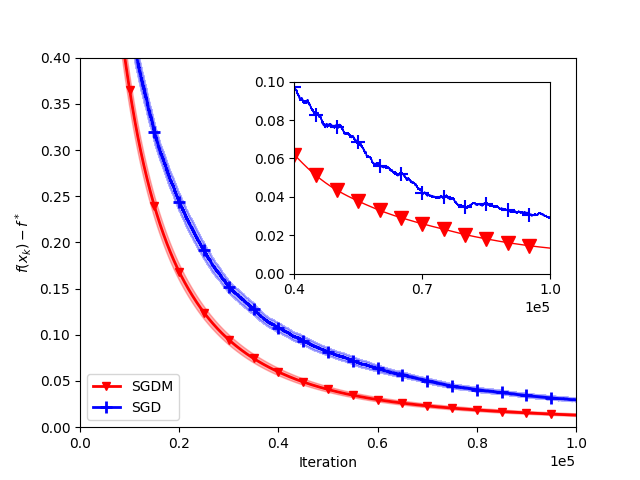
(a) Artificial Experiment

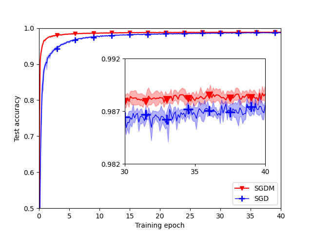
(b) MNIST

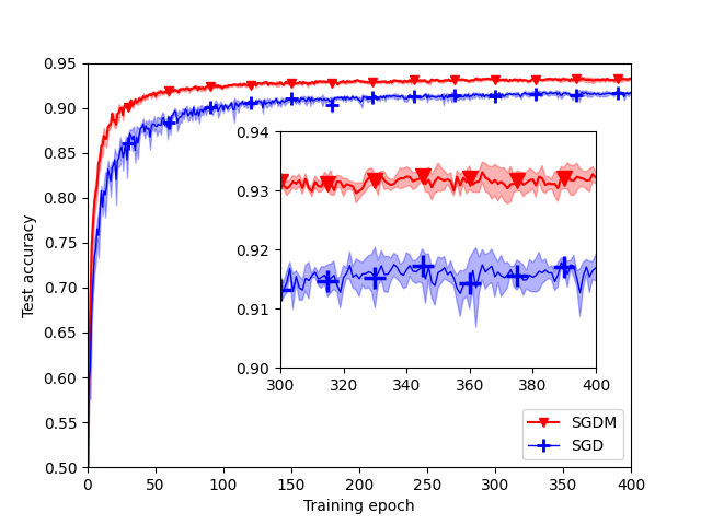
(c) CIFAR-10

Figure 2: Results of the artificial experiment (Figure 2(a)), image classification on MNIST (Figure 2(b)) and CIFAR-10 (Figure 2(c)). The solid lines in the main plot of all figures are obtained through averaging $10$ independent runs, and the variance regions are represented by shaded areas above and below the solid lines. The subplot in Figure 2(a) presents an individual run, and the subplots in Figure 2(b) and 2(c) are zoomed in to provide better views of the last $1/4$ training processes.

Firstly, we investigate the performance of SGDM on a $10$-dimensional quadratic optimization problem. In this artificial experiment, a Gaussian noise is added to each gradient output. For SGD, we use the classic stepsize $\eta_{k}=\frac{1}{\sqrt{k}}$. The results are presented in Figure 2(a). We observe that SGDM converges faster than SGD. Furthermore, the gradient noise in each iteration of SGDM is multiplied by a factor of order $\widetilde{\mathcal{O}}\left(\frac{1}{k^{\frac{3}{2}}}\right)$, while that of SGD is multiplied by a factor of order $\mathcal{O}\left(\frac{1}{\sqrt{k}}\right)$. This results in the error curve of SGDM being significantly smoother than SGD, as observed from the individual run in the subplot of Figure 2(a). Detailed settings about this experiment and more plots of individual runs are presented in Appendix D.

Then we apply both SGDM and SGD to train neural networks for two image classification tasks, MNIST and CIFAR-10. The model used in the MNIST task is a two-layer CNN, and the model used in the CIFAR-10 task is Resnet-18 (He et al.,, 2016). The learning rate of SGD is tuned by the common hyperparameter selection practice (Bergstra and Bengio,, 2012). More details can be found in Appendix D. The results are presented in Figure 2(b) and 2(c), which confirm the better performance of SGDM. Comparison of individual runs (presented in Appendix D) also shows that the learning curves of SGDM have smaller oscillations than SGD.

6 Conclusion

In this paper, we investigate the continuous-discrete relationship in stochastic optimization field. We propose the SGDM method, and prove that its continuous-time limit is a second-order ODE. We further develop the convergence results for this ODE through a continuous Lyapunov function, and then translate the whole argument to the discrete case. By taking advantage of this framework, we obtain convergence results of SGDM that improve existing works in the field.

Appendix A Additional related works

Stochastic optimization has a long history, with its origins dating back to at least (Robbins and Monro,, 1951; Kiefer and Wolfowitz,, 1952). In recent years, the field has experienced significant growth, driven by the widespread use of mini-batch training in machine learning (Goodfellow et al.,, 2016), which induces stochasticity. Researchers have approached the problem of stochastic optimization from various perspectives. For instance, Johnson and Zhang, (2013), Allen-Zhu and Hazan, (2016), Allen-Zhu, (2017), Allen-Zhu, (2018), and Ge et al., (2019) investigated algorithms that only use full-batch training sporadically for finite-sum optimization problems. This class of algorithms are commonly known as Stochastic Variance Reduced Gradient (SVRG). Li and Orabona, (2019), Ward et al., (2020), and Faw et al., (2022) provided theoretical results for stochastic gradient methods with adaptive stepsizes. Zhang et al., (2020) demonstrated, both theoretically and empirically, that the heavy-tailed nature of gradient noise contributes to the advantage of adaptive gradient methods over SGD. Gitman et al., (2019) studied the role of momentum in stochastic gradient methods. Karimi et al., (2016) and Madden et al., (2020) proved the convergence of stochastic gradient methods under the PL condition. Sebbouh et al., (2021) showed the almost sure convergence of SGD and the stochastic heavy-ball method. The convergence of stochastic gradient methods in expectation is also well studied. Shamir and Zhang, (2013) studied the last-iterate convergence of SGD in expectation for non-smooth objective functions, and provided an optimal averaging scheme. Yan et al., (2018) presented a unified convergence analysis for stochastic momentum methods. Assran and Rabbat, (2020) studied the convergence of Nesterov’s accelerated gradient method in stochastic settings. Liu et al., (2020) also provided an improved convergence analysis in expectation of a momentumized SGD, and proved the benefit of using the multistage strategy. Another line of research has centered around Langevin dynamics (e.g., Hsieh et al.,, 2018; Xu et al.,, 2018). With roots in the ergodic analysis of simulated annealing and related algorithms (Chiang et al.,, 1987; Gelfand and Mitter,, 1991; Bélisle,, 1992; Granville et al.,, 1994; Mattingly et al.,, 2010), recent studies in the machine learning community have primarily focused on specific tasks, such as statistical sampling for machine learning (Welling and Teh,, 2011; Zou et al.,, 2019; Chatterji et al.,, 2020; Mou et al.,, 2021) and Riemannian learning (Cheng et al.,, 2022). Notably, Langevin dynamics are not directly connected to the stochastic optimization algorithm studied in this paper. This distinction arises from the fact that Langevin dynamics correspond to the Euler scheme for a SDE, while the continuous-time limit of SGDM algorithm is an ODE.

Appendix B Proof of Theorem 5

For the proof of Theorem 5, we need the following two concentration results.

Lemma 5.

Let $\theta_{1},\cdots,\theta_{k}$ be a sequence of i.i.d. random variables, $\Phi_{l}=\Phi\left(\theta_{[l]}\right)$ be deterministic functions of $\theta_{[l]}=(\theta_{1},\cdots,\theta_{l})$, and $c_{1},\cdots,c_{k}$ be a sequence of positive numbers. If the inequality

$$\mathbb{E}\left[\left.\exp\left(\frac{\Phi_{l}^{2}}{\sigma^{2}}\right)\right|\theta_{[l-1]}\right]\leq\exp(1)$$

holds for each $l\leq k$, then for any $\Omega\geq 0$, we have

$$\mathbb{P}\left(\sum_{l=1}^{k}c_{l}\Phi_{l}^{2}\geq(1+\Omega)\sum_{l=1}^{k}c_{l}\sigma^{2}\right)\leq\exp(-\Omega).$$

Proof.

Since $f(x)=e^{x}$ is convex, we have

$$\mathbb{E}\left[\exp\left(\frac{\sum_{l=1}^{k}c_{l}\Phi_{l}^{2}}{\sum_{l=1}^{k}c_{l}\sigma^{2}}\right)\right]=\mathbb{E}\left[\exp\left(\frac{\sum_{l=1}^{k}c_{l}\sigma^{2}\frac{\Phi_{l}^{2}}{\sigma^{2}}}{\sum_{l=1}^{k}c_{l}\sigma^{2}}\right)\right]\leq\frac{\sum_{l=1}^{k}c_{l}\sigma^{2}\mathbb{E}\left[\exp\left(\frac{\Phi_{l}^{2}}{\sigma^{2}}\right)\right]}{\sum_{l=1}^{k}c_{l}\sigma^{2}}.$$

For each $l$, we have $\mathbb{E}\left[\exp\left(\frac{\Phi_{l}^{2}}{\sigma^{2}}\right)\right]=\mathbb{E}\left[\mathbb{E}\left[\left.\exp\left(\frac{\Phi_{l}^{2}}{\sigma^{2}}\right)\right|\theta_{[l-1]}\right]\right]\leq\exp(1)$, and thus

$$\mathbb{E}\left[\exp\left(\frac{\sum_{l=1}^{k}c_{l}\Phi_{l}^{2}}{\sum_{l=1}^{k}c_{l}\sigma^{2}}\right)\right]\leq\exp(1).$$

Then Markov’s inequality yields that the inequality

$$\mathbb{P}\left(\exp\left(\frac{\sum_{l=1}^{k}c_{l}\Phi_{l}^{2}}{\sum_{l=1}^{k}c_{l}\sigma^{2}}\right)\geq\delta\right)\leq\frac{\exp(1)}{\delta}$$

holds for any $\delta>0$. Therefore, for any $\Omega\geq 0$, by letting $\delta=\exp(1+\Omega)$ and using the monotonicity of $f(x)=e^{x}$, we conclude that

$$\mathbb{P}\left(\sum_{l=1}^{k}c_{l}\Phi_{l}^{2}\geq(1+\Omega)\sum_{l=1}^{k}c_{l}\sigma^{2}\right)\leq\frac{\exp(1)}{\exp(1+\Omega)}=\exp(-\Omega).\qed$$

Lemma 6.

Let $\theta_{1},\cdots,\theta_{k}$ be a sequence of i.i.d. random variables, $\Gamma_{l}=\Gamma\left(\theta_{[l]}\right)$ and $\Delta_{l}=\Delta\left(\theta_{[l]}\right)$ be deterministic functions of $\theta_{[l]}=(\theta_{1},\cdots,\theta_{l})$, and $c_{1},\cdots,c_{k}$ be a sequence of positive numbers such that:

1. $\mathbb{E}[\Gamma_{l}|\theta_{[l-1]}]=0$,

2. $|\Gamma_{l}|\leq c_{l}\Delta_{l}$,

3. $\mathbb{E}\left[\left.\exp\left(\frac{\Delta_{l}^{2}}{\sigma^{2}}\right)\right|\theta_{[l-1]}\right]\leq\exp(1)$,

holds for each $l\leq k$. Then for any $\Omega\geq 0$, we have

$$\mathbb{P}\left(\sum_{l=1}^{k}\Gamma_{l}\geq\sqrt{3\Omega\sum_{l=1}^{k}c_{l}^{2}\sigma^{2}}\right)\leq\exp(-\Omega).$$

Lemma 6 has appeared in Lan et al., (2012) in different forms. Below we provide a proof for completeness.

Proof of Lemma 6.

Since $\exp(x)\leq x+\exp\left(\frac{9x^{2}}{16}\right)$ for any $x$, we have

$$\mathbb{E}\left[\left.\exp\left(\frac{\lambda\Gamma_{l}}{c_{l}\sigma}\right)\right|\theta_{[l-1]}\right]\leq\mathbb{E}\left[\left.\frac{\lambda\Gamma_{l}}{c_{l}\sigma}\right|\theta_{[l-1]}\right]+\mathbb{E}\left[\left.\exp\left(\frac{9\lambda^{2}\Gamma_{l}^{2}}{16c_{l}^{2}\sigma^{2}}\right)\right|\theta_{[l-1]}\right]\leq\mathbb{E}\left[\left.\exp\left(\frac{9\lambda^{2}\Delta_{l}^{2}}{16\sigma^{2}}\right)\right|\theta_{[l-1]}\right],$$

for any $\lambda$, where the second inequality uses the condition 1 and 2. From the concavity of $f(x)=x^{p}$ for $0<p\leq 1$, we further have

$$\mathbb{E}\left[\left.\exp\left(\frac{\lambda\Gamma_{l}}{c_{l}\sigma}\right)\right|\theta_{[l-1]}\right]\leq\left(\mathbb{E}\left[\left.\exp\left(\frac{\Delta_{l}^{2}}{\sigma^{2}}\right)\right|\theta_{[l-1]}\right]\right)^{\frac{9\lambda^{2}}{16}}\leq\exp\left(\frac{9\lambda^{2}}{16}\right),$$ (51)

for any $0<\lambda\leq\frac{4}{3}$, where the second inequality uses condition 3. On the other hand, since $\lambda x\leq\frac{3}{8}\lambda^{2}+\frac{2}{3}x^{2}$ for any $\lambda$ and $x$, we have

$$\begin{split}\mathbb{E}\left[\left.\exp\left(\frac{\lambda\Gamma_{l}}{c_{l}\sigma}\right)\right|\theta_{[l-1]}\right]\leq&\exp\left(\frac{3\lambda^{2}}{8}\right)\mathbb{E}\left[\left.\exp\left(\frac{2\Gamma_{l}^{2}}{3c_{l}^{2}\sigma^{2}}\right)\right|\theta_{[l-1]}\right]\\ \leq&\exp\left(\frac{3\lambda^{2}}{8}\right)\mathbb{E}\left[\left.\exp\left(\frac{2\Delta_{l}^{2}}{3\sigma^{2}}\right)\right|\theta_{[l-1]}\right]\\ \leq&\exp\left(\frac{3\lambda^{2}}{8}+\frac{2}{3}\right),\end{split}$$ (52)

for any $\lambda$, where the third inequality uses the concavity of $f(x)=x^{\frac{2}{3}}$ and the condition 3. Combining (51) and (52) yields that

$$\mathbb{E}\left[\left.\exp\left(\frac{\lambda\Gamma_{l}}{c_{l}\sigma}\right)\right|\theta_{[l-1]}\right]\leq\exp\left(\frac{3\lambda^{2}}{4}\right),$$

for any $\lambda$, and thus

$$\mathbb{E}\left[\left.\exp\left(\lambda\Gamma_{l}\right)\right|\theta_{[l-1]}\right]\leq\exp\left(\frac{3\lambda^{2}c_{l}^{2}\sigma^{2}}{4}\right),$$

for any $\lambda$. Then we have

$$\mathbb{E}\left[\exp\left(\sum_{l=1}^{k}\lambda\Gamma_{l}\right)\right]=\mathbb{E}\left[\exp\left(\sum_{l=1}^{k-1}\lambda\Gamma_{l}\right)\mathbb{E}\left[\left.\exp\left(\lambda\Gamma_{l}\right)\right|\theta_{[l-1]}\right]\right]\leq\exp\left(\frac{3\lambda^{2}c_{l}^{2}\sigma^{2}}{4}\right)\mathbb{E}\left[\exp\left(\sum_{l=1}^{k-1}\lambda\Gamma_{l}\right)\right],$$

and hence

$$\mathbb{E}\left[\exp\left(\sum_{l=1}^{k}\lambda\Gamma_{l}\right)\right]\leq\exp\left(\frac{3\lambda^{2}\sum_{l=1}^{k}c_{l}^{2}\sigma^{2}}{4}\right).$$

Therefore, the Markov’s inequality gives that for any $\lambda>0$ and $\Omega\geq 0$,

$$\mathbb{P}\left(\sum_{l=1}^{k}\Gamma_{l}\geq\sqrt{3\Omega\sum_{l=1}^{k}c_{l}^{2}\sigma^{2}}\right)= \mathbb{P}\left(\exp\left(\sum_{l=1}^{k}\lambda\Gamma_{l}\right)\geq\exp\left(\lambda\sqrt{3\Omega\sum_{l=1}^{k}c_{l}^{2}\sigma^{2}}\right)\right)$$

$$\leq \exp\left(-\lambda\sqrt{3\Omega\sum_{l=1}^{k}c_{l}^{2}\sigma^{2}}\right)\mathbb{E}\left[\exp\left(\sum_{l=1}^{k}\lambda\Gamma_{l}\right)\right]$$

$$\leq \exp\left(\frac{3\lambda^{2}\sum_{l=1}^{k}c_{l}^{2}\sigma^{2}}{4}-\lambda\sqrt{3\Omega\sum_{l=1}^{k}c_{l}^{2}\sigma^{2}}\right).$$

By letting $\lambda=2\sqrt{\frac{\Omega}{3\sum_{l=1}^{k}c_{l}^{2}\sigma^{2}}}$, we conclude that

$$\mathbb{P}\left(\sum_{l=1}^{k}\Gamma_{l}\geq\sqrt{3\Omega\sum_{l=1}^{k}c_{l}^{2}\sigma^{2}}\right)\leq\exp(-\Omega).\qed$$

With Lemma 5 and 6 in place, we present the proof of Theorem 5.

Theorem 5. Let Assumption 1, 2 and 3 hold. For any $0<\beta\leq\frac{1}{e}$, the sequence $\{x_{k}\}$ generated by SGDM (29) with stepsize $\eta_{k}=\frac{1}{16L^{2}\log^{2}(k+2)}$ and initialization $x_{0}=x_{1}$ satisfies

$$\mathbb{P}\left(f(x_{k})-f(x^{*})\leq\frac{8Lc_{1}((c_{2}+c_{3}\log k)\sigma^{2}+c_{4})\log(k+2)\log\frac{1}{\beta}}{\sqrt{k+1}}\right)\geq 1-\beta$$

for any $k$, where $c_{1}=\max\{\mathcal{E}(0),\sum_{i=1}^{\infty}\frac{\eta_{i}}{i}\}$, $\mathcal{E}(0)=\|x_{0}-x^{*}\|^{2}+4\eta_{0}(f(x_{0})-f^{*})$, $c_{2}=54$, $c_{3}=26$ and $c_{4}=2$.

Proof.

Lemma 3 yields that

$$\mathcal{E}(k)-\mathcal{E}(k-1)\leq \frac{4\eta_{k}}{k}\left\|g(x_{k},\xi_{k})\right\|^{2}-\frac{2}{L}\sqrt{\frac{\eta_{k}}{k}}\|\nabla f(x_{k})\|^{2}+4\sqrt{\frac{\eta_{k}}{k}}\langle\nabla f(x_{k})-g(x_{k},\xi_{k}),\tau_{k}\rangle$$

$$\leq \frac{8\eta_{k}}{k}\left\|\theta_{k}\right\|^{2}+\frac{8\eta_{k}}{k}\|\nabla f(x_{k})\|^{2}-\frac{2}{L}\sqrt{\frac{\eta_{k}}{k}}\|\nabla f(x_{k})\|^{2}+4\sqrt{\frac{\eta_{k}}{k}}\langle\theta_{k},\tau_{k}\rangle$$

$$\leq \frac{8\eta_{k}}{k}\left\|\theta_{k}\right\|^{2}+4\sqrt{\frac{\eta_{k}}{k}}\langle\theta_{k},\tau_{k}\rangle,$$

where $\tau_{k}=k(x_{k}-x_{k-1})+p(x_{k}-x^{*})$, $\theta_{k}=\nabla f(x_{k})-g(x_{k},\xi_{k})$, and the third inequality follows from $\eta_{k}\leq\frac{k}{16L^{2}}$ for $k\geq 1$. Summing the above inequality over $k$ gives

$$\mathcal{E}(k)\leq\mathcal{E}(0)+\sum_{i=1}^{k}\frac{8\eta_{i}}{i}\|\theta_{i}\|^{2}+\sum_{i=1}^{k}4\sqrt{\frac{\eta_{i}}{i}}\langle\theta_{i},\tau_{i}\rangle.$$ (53)

In the remaining part of the proof, we establish the high probability bound of $\mathcal{E}(k)$ based on (53). More specifically, via induction we prove that for all $l=0,\cdots,k$, with probability at least $1-\frac{l\beta}{k}$, the following statement holds: inequalities

$$\mathcal{E}(m)\leq 8c_{1}((c_{2}+c_{3}\log k)\sigma^{2}+c_{4})\log\frac{1}{\beta}$$ (54)

hold for $m=0,\cdots,l$ simultaneously. For convenience, we define the event when this statement holds as $E_{l}$. Then our goal is to show that $\mathbb{P}(E_{l})\geq 1-\frac{l\beta}{k}$ for all $l\leq k$.

For $l=0$, $E_{0}$ holds with probability $1$ since $c_{1}\geq\mathcal{E}(0)$, $c_{4}=2$ and $\log\frac{1}{\beta}\geq 1$. Next, assume that for some $l={l_{0}}-1\leq k-1$ we have $\mathbb{P}(E_{{l_{0}}-1})\geq 1-\frac{({l_{0}}-1)\beta}{k}$. Then we show that $\mathbb{P}(E_{l_{0}})\geq 1-\frac{{l_{0}}\beta}{k}$.

To do this, our critical observation is that the norm of $\tau_{k+1}=x_{k+1}+(k+1)(x_{k+1}-x_{k})-px^{*}$ is contained in the Lyapunov function $\mathcal{E}(k)$. Thus, under our induction hypothesis, we can apply the inequality (53) to $\mathcal{E}({l_{0}})$, and bound the third term on the RHS, $\sum_{i=1}^{l_{0}}L4\sqrt{\frac{\eta_{i}}{i}}\langle\theta_{i},\tau_{i}\rangle$, by using a concentration inequality. Firstly, event $E_{{l_{0}}-1}$ implies

$$\|\tau_{m+1}\|^{2}\leq\mathcal{E}(m)\leq 8c_{1}((c_{2}+c_{3}\log k)\sigma^{2}+c_{4})\log\frac{1}{\beta},$$ (55)

for each $0\leq m\leq{l_{0}}-1$. Based on (55), we show that (54) holds for $m={l_{0}}$ with high probability. We introduce a new random variable

$$\begin{split}\nu_{m}=\left\{\begin{aligned} &\tau_{m},\text{ if $\|\tau_{m}\|\leq\sqrt{8c_{1}((c_{2}+c_{3}\log k)\sigma^{2}+c_{4})\log\frac{1}{\beta}}$,}\\ &0,\text{ otherwise,}\end{aligned}\right.\end{split}$$ (56)

for each $1\leq m\leq{l_{0}}$. From (53), (55) and (56), $E_{{l_{0}}-1}$ implies that

$$\mathcal{E}({l_{0}})\leq\mathcal{E}(0)+\sum_{i=1}^{l_{0}}\frac{8\eta_{i}}{i}\|\theta_{i}\|^{2}+\sum_{i=1}^{l_{0}}4\sqrt{\frac{\eta_{i}}{i}}\langle\theta_{i},\nu_{i}\rangle.$$ (57)

From $\log\frac{1}{\beta}>1$ and $c_{1}\geq\mathcal{E}(0)$, dividing both sides of (57) by $8c_{1}\log\frac{1}{\beta}$ yields that

$$\begin{split}\frac{\mathcal{E}({l_{0}})}{8c_{1}\log\frac{1}{\beta}}\leq 1+\underbrace{\sum_{i=1}^{l_{0}}\frac{\eta_{i}}{c_{1}\log\frac{1}{\beta}\cdot i}\|\theta_{i}\|^{2}}_{\text{\char 172}}+\underbrace{\sum_{i=1}^{l_{0}}\frac{1}{c_{1}\log\frac{1}{\beta}}\sqrt{\frac{\eta_{i}}{i}}\langle\theta_{i},\nu_{i}\rangle}_{\text{\char 173}}.\end{split}$$ (58)

It remains to provide bounds for ① and ②.

For ①, Lemma 5 shows that

$$\mathbb{P}\left(\sum_{i=1}^{l_{0}}\frac{\eta_{i}}{c_{1}\log\frac{1}{\beta}\cdot i}\|\theta_{i}\|^{2}\geq(1+\Omega)\sigma^{2}\sum_{i=1}^{l_{0}}\frac{\eta_{i}}{c_{1}\log\frac{1}{\beta}\cdot i}\right)\leq e^{-\Omega}.$$

From $\log\frac{1}{\beta}\geq 1$ and $\sum_{i=1}^{l_{0}}\frac{\eta_{i}}{i}\leq c_{1}$, we have

$$\left(1+\log\frac{2k}{\beta}\right)\sum_{i=1}^{l_{0}}\frac{\eta_{i}}{c_{1}\log\frac{1}{\beta}\cdot i}\leq 3+\log k.$$

Therefore, by letting $\Omega=\log\frac{2k}{\beta}$, we have

$$\mathbb{P}\left(\sum_{i=1}^{l_{0}}\frac{\eta_{i}}{c_{1}\log\frac{1}{\beta}\cdot i}\|\theta_{i}\|^{2}\geq(3+\log k)\sigma^{2}\right)\leq\frac{\beta}{2k}.$$ (59)

For ②, from (56) we have

$$\left|\frac{1}{c_{1}\log\frac{1}{\beta}}\sqrt{\frac{\eta_{i}}{i}}\langle\theta_{i},\nu_{i}\rangle\right|\leq\frac{1}{c_{1}\log\frac{1}{\beta}}\sqrt{\frac{\eta_{i}}{i}}\sqrt{8c_{1}((c_{2}+c_{3}\log k)\sigma^{2}+c_{4})\log\frac{1}{\beta}}\cdot\|\theta_{i}\|.$$

Therefore, Lemma 6 yields that

$$\mathbb{P}\left(\sum_{i=1}^{l_{0}}\frac{1}{c_{1}\log\frac{1}{\beta}}\sqrt{\frac{\eta_{i}}{i}}\langle\theta_{i+1},\nu_{i+1}\rangle\geq\frac{\sqrt{3\Omega}\sigma}{c_{1}\sqrt{\log\frac{1}{\beta}}}\sqrt{\sum_{i=1}^{l_{0}}\frac{8c_{1}\eta_{i}}{i}((c_{2}+c_{3}\log k)\sigma^{2}+c_{4})}\right)\leq e^{-\Omega}.$$

Calculation shows that

$$\frac{\sqrt{\log\frac{2k}{\beta}}}{c_{1}\sqrt{\log\frac{1}{\beta}}}\sqrt{\sum_{i=1}^{l_{0}}\frac{8c_{1}\eta_{i}}{i}((c_{2}+c_{3}\log k)\sigma^{2}+c_{4})}= \sqrt{\frac{\log\frac{2k}{\beta}}{\log\frac{1}{\beta}}}\sqrt{(c_{2}+c_{3}\log k)\sigma^{2}+c_{4}}\sqrt{\frac{8\sum_{i=1}^{l_{0}}\frac{\eta_{i}}{i}}{c_{1}}}$$

$$\leq \sqrt{8(2+\log k)((c_{2}+c_{3}\log k)\sigma^{2}+c_{4})},$$

where the last inequality follows from $\log\frac{1}{\beta}\geq 1$ and $\sum_{i=1}^{l_{0}}\frac{\eta_{i}}{i}\leq c_{1}$. Therefore, by letting $\Omega=\log\frac{2k}{\beta}$, we have

$$\begin{split}\mathbb{P}\left(\sum_{i=1}^{l_{0}}\frac{1}{c_{1}\log\frac{1}{\beta}}\sqrt{\frac{\eta_{i}}{i}}\langle\theta_{i},\nu_{i}\rangle\geq\sqrt{24(2+\log k)\sigma^{2}((c_{2}+c_{3}\log k)\sigma^{2}+c_{4})}\right)\leq\frac{\beta}{2k}.\end{split}$$ (60)

We let

$$E_{\text{\char 172}}=\left\{\sum_{i=1}^{l_{0}}\frac{\eta_{i}}{c_{1}\log\frac{1}{\beta}\cdot i}\|\theta_{i}\|^{2}<(3+\log k)\sigma^{2}\right\}$$

and

$$E_{\text{\char 173}}=\left\{\sum_{i=1}^{l_{0}}\frac{1}{c_{1}\log\frac{1}{\beta}}\sqrt{\frac{\eta_{i}}{i}}\langle\theta_{i},\nu_{i}\rangle<\sqrt{24(2+\log k)\sigma^{2}((c_{2}+c_{3}\log k)\sigma^{2}+c_{4})}\right\}.$$

Then under event $E_{{l_{0}}-1}\cap E_{\text{\char 172}}\cap E_{\text{\char 173}}$, (58) yields that

$$\frac{\mathcal{E}({l_{0}})}{8c_{1}\log\frac{1}{\beta}}\leq 1+(3+\log k)\sigma^{2}+\sqrt{24(2+\log k)\sigma^{2}((c_{2}+c_{3}\log k)\sigma^{2}+c_{4})}.$$

From $c_{2}=54$, $c_{3}=26$ and $c_{4}=2$, we have

$$\sqrt{24(2+\log k)\sigma^{2}((c_{2}+c_{3}\log k)\sigma^{2}+c_{4})}\leq(c_{2}+c_{3}\log k)\sigma^{2}+c_{4}-(1+(3+\log k)\sigma^{2}),$$

and thus

$$\frac{\mathcal{E}({l_{0}})}{8c_{1}\log\frac{1}{\beta}}\leq(c_{2}+c_{3}\log k)\sigma^{2}+c_{4}.$$ (61)

Moreover, (59), (60) and the induction hypothesis $\mathbb{P}(E_{{l_{0}}-1})\geq 1-\frac{({l_{0}}-1)\beta}{k}$ show that

$$\mathbb{P}(E_{{l_{0}}-1}\cap E_{\text{\char 172}}\cap E_{\text{\char 173}})\geq 1-\left(\frac{({l_{0}}-1)\beta}{k}+\frac{\beta}{2k}+\frac{\beta}{2k}\right)=1-\frac{{l_{0}}\beta}{k}.$$

Thus, by (61) and the definition of $E_{l_{0}}$, we have

$$\mathbb{P}(E_{l_{0}})\geq\mathbb{P}(E_{{l_{0}}-1}\cap E_{\text{\char 172}}\cap E_{\text{\char 173}})\geq 1-\frac{{l_{0}}\beta}{k}.$$

As a consequence, the induction yields that $\mathbb{P}(E_{l})\geq 1-\frac{l\beta}{k}$ for each $l\leq k$. Specifically, the inequality

$$\mathcal{E}(k)\leq 8c_{1}((c_{2}+c_{3}\log k)\sigma^{2}+c_{4})\log\frac{1}{\beta}$$ (62)

holds with probability at least $1-\beta$. Since (62) and (30) implies

$$f(x_{k})-f(x^{*})\leq\frac{8Lc_{1}((c_{2}+c_{3}\log k)\sigma^{2}+c_{4})\log(k+2)\log\frac{1}{\beta}}{\sqrt{k+1}},$$

the proof of Theorem 5 is completed. ∎

Appendix C Proof of Remark 1

Theorem 5 shows that for each $1\leq k\leq k_{0}-1$, there exists event $\widetilde{E}_{k}$ such that $\mathbb{P}(\widetilde{E}_{k})\geq 1-\frac{\beta}{k_{0}}$ and

$$\begin{split}f(x_{k}(\omega))-f^{*}&\leq\frac{8Lc_{1}((c_{2}+c_{3}\log k)\sigma^{2}+c_{4})\log(k+2)\log\frac{k_{0}}{\beta}}{\sqrt{k+1}}\\ &\leq\frac{C_{0}\log k_{0}\cdot\log(k+2)\log\frac{k_{0}}{\beta}}{\sqrt{k}},\end{split}$$ (63)

for any $\omega\in\widetilde{E}_{k}$, where $C_{0}=(16c_{1}((c_{2}+c_{3})\sigma^{2}+c_{4})+4)L$. Then Theorem 6 and (63) give that

$$\mathbb{P}\left(\forall k\geq 1,\;f(x_{k})-f(x^{*})\leq\frac{C_{0}\log k_{0}(\log k_{0}+\log\frac{1}{\beta})\log(k+2)}{\sqrt{k}}\right)\geq\mathbb{P}\left(\bigcap_{k=1}^{k_{0}-1}\widetilde{E}_{k}\bigcap\widehat{E}\right)\geq 1-2\beta.$$

Appendix D Additional Details and Results for the Experiments

In our artificial experiment, the objective function is $f(x)=\frac{1}{2}x^{\mathsf{T}}Ax$, and $A\in\mathbb{R}^{10\times 10}$ is randomly generated. When the algorithm calls the gradient oracle at $x\in\mathbb{R}^{10}$, it outputs a stochastic gradient $Ax+\xi$, where $\xi\sim\mathcal{N}(0,100\cdot I_{10})$.

In the two image classification tasks, we set $\eta=0.2$ for SGDM. The stepsize of SGD is tuned over $[10^{-4},1]$ by grid search (Bergstra and Bengio,, 2012), and we report the results with the best choices, $0.005$ for the MNIST task and $0.01$ for the CIFAR-10 task. In the MNIST task, the model is trained for $40$ epochs, while in the CIFAR-10 task, the model is trained for $400$ epochs.

In Figure 3, 4 and 5 we present another three individual runs of SGDM and SGD for the three experiments. All these results confirm that SGDM has faster convergence and smaller oscillations than SGD.

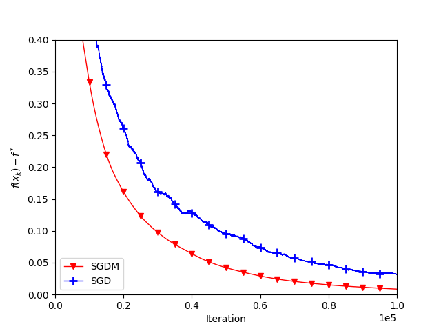
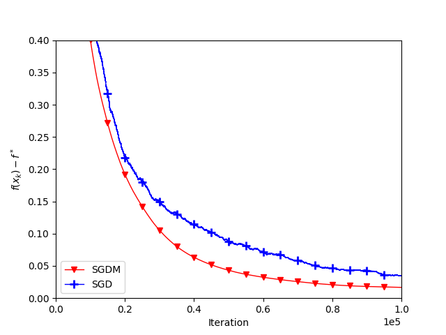
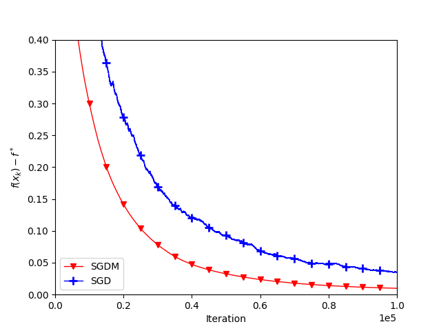
Figure 3: Three individual runs of SGDM and SGD on the artificial experiment.

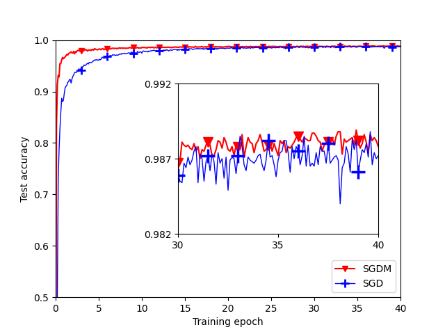
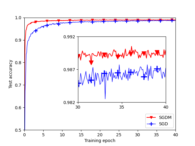
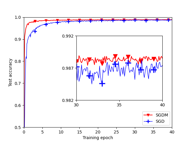
Figure 4: Three individual runs of SGDM and SGD on the MNIST task. The subplots are zoomed in to provide better views of the last $1/4$ training processes.

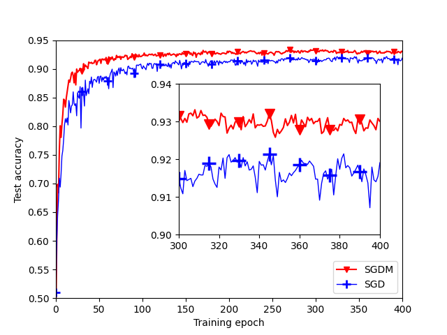
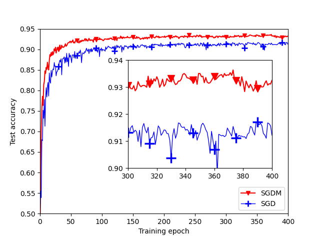
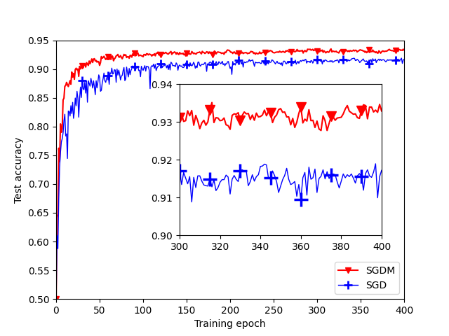
Figure 5: Three individual runs of SGDM and SGD on the CIFAR-10 task. The subplots are zoomed in to provide better views of the last $1/4$ training processes.

References

• Agarwal et al., (2012) Agarwal, A., Bartlett, P. L., Ravikumar, P., and Wainwright, M. J. (2012). Information-theoretic lower bounds on the oracle complexity of stochastic convex optimization. IEEE Transactions on Information Theory, 58(5):3235–3249.
• Allen-Zhu, (2017) Allen-Zhu, Z. (2017). Katyusha: The first direct acceleration of stochastic gradient methods. In Proceedings of the 49th Annual ACM SIGACT Symposium on Theory of Computing, pages 1200–1205.
• Allen-Zhu, (2018) Allen-Zhu, Z. (2018). Katyusha X: Simple momentum method for stochastic sum-of-nonconvex optimization. In International Conference on Machine Learning, pages 179–185. PMLR.
• Allen-Zhu and Hazan, (2016) Allen-Zhu, Z. and Hazan, E. (2016). Variance reduction for faster non-convex optimization. In International conference on machine learning, pages 699–707. PMLR.
• Assran and Rabbat, (2020) Assran, M. and Rabbat, M. (2020). On the convergence of nesterov’s accelerated gradient method in stochastic settings. In International Conference on Machine Learning, pages 410–420. PMLR.
• Bélisle, (1992) Bélisle, C. J. (1992). Convergence theorems for a class of simulated annealing algorithms on $\mathbb{R}^{d}$. Journal of Applied Probability, 29(4):885–895.
• Bergstra and Bengio, (2012) Bergstra, J. and Bengio, Y. (2012). Random search for hyper-parameter optimization. Journal of machine learning research, 13(2).
• Chatterji et al., (2020) Chatterji, N., Diakonikolas, J., Jordan, M. I., and Bartlett, P. (2020). Langevin Monte Carlo without smoothness. In International Conference on Artificial Intelligence and Statistics, pages 1716–1726. PMLR.
• Cheng et al., (2020) Cheng, X., Yin, D., Bartlett, P., and Jordan, M. (2020). Stochastic gradient and langevin processes. In International Conference on Machine Learning, pages 1810–1819. PMLR.
• Cheng et al., (2022) Cheng, X., Zhang, J., and Sra, S. (2022). Efficient sampling on riemannian manifolds via langevin mcmc. Advances in Neural Information Processing Systems, 35:5995–6006.
• Chiang et al., (1987) Chiang, T.-S., Hwang, C.-R., and Sheu, S. J. (1987). Diffusion for global optimization in $\mathbb{R}^{n}$. SIAM Journal on Control and Optimization, 25(3):737–753.
• Cutkosky and Mehta, (2021) Cutkosky, A. and Mehta, H. (2021). High-probability bounds for non-convex stochastic optimization with heavy tails. Advances in Neural Information Processing Systems, 34:4883–4895.
• Difonzo et al., (2022) Difonzo, F. V., Kungurtsev, V., and Marecek, J. (2022). Stochastic langevin differential inclusions with applications to machine learning. arXiv preprint arXiv:2206.11533.
• Faw et al., (2022) Faw, M., Tziotis, I., Caramanis, C., Mokhtari, A., Shakkottai, S., and Ward, R. (2022). The power of adaptivity in sgd: Self-tuning step sizes with unbounded gradients and affine variance. In Conference on Learning Theory, pages 313–355. PMLR.
• Ge et al., (2019) Ge, R., Li, Z., Wang, W., and Wang, X. (2019). Stabilized SVRG: Simple variance reduction for nonconvex optimization. In Conference on learning theory, pages 1394–1448. PMLR.
• Gelfand and Mitter, (1991) Gelfand, S. B. and Mitter, S. K. (1991). Recursive stochastic algorithms for global optimization in $\mathbb{R}^{d}$. SIAM Journal on Control and Optimization, 29(5):999–1018.
• Ghadimi and Lan, (2013) Ghadimi, S. and Lan, G. (2013). Stochastic first-and zeroth-order methods for nonconvex stochastic programming. SIAM Journal on Optimization, 23(4):2341–2368.
• Gitman et al., (2019) Gitman, I., Lang, H., Zhang, P., and Xiao, L. (2019). Understanding the role of momentum in stochastic gradient methods. Advances in Neural Information Processing Systems, 32.
• Goodfellow et al., (2016) Goodfellow, I. J., Bengio, Y., and Courville, A. (2016). Deep Learning. MIT Press, Cambridge, MA, USA.
• Gorbunov et al., (2020) Gorbunov, E., Danilova, M., and Gasnikov, A. (2020). Stochastic optimization with heavy-tailed noise via accelerated gradient clipping. Advances in Neural Information Processing Systems, 33:15042–15053.
• Granville et al., (1994) Granville, V., Krivánek, M., and Rasson, J.-P. (1994). Simulated annealing: A proof of convergence. IEEE transactions on pattern analysis and machine intelligence, 16(6):652–656.
• Harvey et al., (2019) Harvey, N. J., Liaw, C., Plan, Y., and Randhawa, S. (2019). Tight analyses for non-smooth stochastic gradient descent. In Conference on Learning Theory, pages 1579–1613. PMLR.
• He et al., (2016) He, K., Zhang, X., Ren, S., and Sun, J. (2016). Deep residual learning for image recognition. In Proceedings of the IEEE conference on computer vision and pattern recognition, pages 770–778.
• He et al., (2018) He, L., Meng, Q., Chen, W., Ma, Z.-M., and Liu, T.-Y. (2018). Differential equations for modeling asynchronous algorithms. In Proceedings of the 27th International Joint Conference on Artificial Intelligence, pages 2220–2226.
• Helmke and Moore, (1996) Helmke, U. and Moore, J. (1996). Optimization and dynamical systems. Proceedings of the IEEE, 84(6):907.
• Howard et al., (2021) Howard, S. R., Ramdas, A., McAuliffe, J., and Sekhon, J. (2021). Time-uniform, nonparametric, nonasymptotic confidence sequences. The Annals of Statistics, 49(2).
• Hsieh et al., (2018) Hsieh, Y.-P., Kavis, A., Rolland, P., and Cevher, V. (2018). Mirrored Langevin dynamics. Advances in Neural Information Processing Systems, 31.
• Jain et al., (2021) Jain, P., Nagaraj, D. M., and Netrapalli, P. (2021). Making the last iterate of SGD information theoretically optimal. SIAM Journal on Optimization, 31(2):1108–1130.
• Jamieson et al., (2014) Jamieson, K., Malloy, M., Nowak, R., and Bubeck, S. (2014). lil’ucb: An optimal exploration algorithm for multi-armed bandits. In Conference on Learning Theory, pages 423–439. PMLR.
• Jamieson and Talwalkar, (2016) Jamieson, K. and Talwalkar, A. (2016). Non-stochastic best arm identification and hyperparameter optimization. In Artificial intelligence and statistics, pages 240–248. PMLR.
• Johnson and Zhang, (2013) Johnson, R. and Zhang, T. (2013). Accelerating stochastic gradient descent using predictive variance reduction. Advances in neural information processing systems, 26.
• Karimi et al., (2016) Karimi, H., Nutini, J., and Schmidt, M. (2016). Linear convergence of gradient and proximal-gradient methods under the polyak-łojasiewicz condition. In Joint European Conference on Machine Learning and Knowledge Discovery in Databases, pages 795–811. Springer.
• Kaufmann and Koolen, (2021) Kaufmann, E. and Koolen, W. M. (2021). Mixture martingales revisited with applications to sequential tests and confidence intervals. The Journal of Machine Learning Research, 22(1):11140–11183.
• Kavis et al., (2021) Kavis, A., Levy, K. Y., and Cevher, V. (2021). High probability bounds for a class of nonconvex algorithms with adagrad stepsize. In International Conference on Learning Representations.
• Kiefer and Wolfowitz, (1952) Kiefer, J. and Wolfowitz, J. (1952). Stochastic estimation of the maximum of a regression function. The Annals of Mathematical Statistics, pages 462–466.
• Krichene et al., (2015) Krichene, W., Bayen, A., and Bartlett, P. L. (2015). Accelerated mirror descent in continuous and discrete time. Advances in neural information processing systems, 28.
• Lai, (1976) Lai, T. L. (1976). On confidence sequences. The Annals of Statistics, pages 265–280.
• Lan, (2012) Lan, G. (2012). An optimal method for stochastic composite optimization. Mathematical Programming, 133(1-2):365–397.
• Lan et al., (2012) Lan, G., Nemirovski, A., and Shapiro, A. (2012). Validation analysis of mirror descent stochastic approximation method. Mathematical programming, 134(2):425–458.
• Li et al., (2018) Li, L., Jamieson, K., DeSalvo, G., Rostamizadeh, A., and Talwalkar, A. (2018). Hyperband: A novel bandit-based approach to hyperparameter optimization. Journal of Machine Learning Research, 18(185):1–52.
• Li et al., (2017) Li, Q., Tai, C., and Weinan, E. (2017). Stochastic modified equations and adaptive stochastic gradient algorithms. In International Conference on Machine Learning, pages 2101–2110. PMLR.
• Li and Liu, (2022) Li, S. and Liu, Y. (2022). High probability guarantees for nonconvex stochastic gradient descent with heavy tails. In International Conference on Machine Learning, pages 12931–12963. PMLR.
• Li and Orabona, (2019) Li, X. and Orabona, F. (2019). On the convergence of stochastic gradient descent with adaptive stepsizes. In The 22nd international conference on artificial intelligence and statistics, pages 983–992. PMLR.
• Li and Orabona, (2020) Li, X. and Orabona, F. (2020). A high probability analysis of adaptive sgd with momentum. In Workshop on Beyond First Order Methods in ML Systems at ICML’20.
• Liu et al., (2020) Liu, Y., Gao, Y., and Yin, W. (2020). An improved analysis of stochastic gradient descent with momentum. Advances in Neural Information Processing Systems, 33:18261–18271.
• Liu et al., (2023) Liu, Z., Nguyen, T. D., Nguyen, T. H., Ene, A., and Nguyen, H. (2023). High probability convergence of stochastic gradient methods. In International Conference on Machine Learning, pages 21884–21914. PMLR.
• Liu and Zhou, (2023) Liu, Z. and Zhou, Z. (2023). Revisiting the last-iterate convergence of stochastic gradient methods. arXiv preprint arXiv:2312.08531.
• Loizou and Richtárik, (2017) Loizou, N. and Richtárik, P. (2017). Linearly convergent stochastic heavy ball method for minimizing generalization error. arXiv preprint arXiv:1710.10737.
• Madden et al., (2020) Madden, L., Dall’Anese, E., and Becker, S. (2020). High-probability convergence bounds for non-convex stochastic gradient descent. arXiv preprint arXiv:2006.05610.
• Mandt et al., (2016) Mandt, S., Hoffman, M., and Blei, D. (2016). A variational analysis of stochastic gradient algorithms. In International conference on machine learning, pages 354–363. PMLR.
• Mattingly et al., (2010) Mattingly, J. C., Stuart, A. M., and Tretyakov, M. V. (2010). Convergence of numerical time-averaging and stationary measures via Poisson equations. SIAM Journal on Numerical Analysis, 48(2):552–577.
• Mou et al., (2021) Mou, W., Ma, Y.-A., Wainwright, M. J., Bartlett, P. L., and Jordan, M. I. (2021). High-order Langevin diffusion yields an accelerated mcmc algorithm. The Journal of Machine Learning Research, 22(1):1919–1959.
• Nazin et al., (2019) Nazin, A. V., Nemirovsky, A. S., Tsybakov, A. B., and Juditsky, A. B. (2019). Algorithms of robust stochastic optimization based on mirror descent method. Automation and Remote Control, 80:1607–1627.
• Nemirovski et al., (2009) Nemirovski, A., Juditsky, A., Lan, G., and Shapiro, A. (2009). Robust stochastic approximation approach to stochastic programming. SIAM Journal on optimization, 19(4):1574–1609.
• Orabona and Jun, (2023) Orabona, F. and Jun, K.-S. (2023). Tight concentrations and confidence sequences from the regret of universal portfolio. IEEE Transactions on Information Theory.
• Orvieto and Lucchi, (2019) Orvieto, A. and Lucchi, A. (2019). Continuous-time models for stochastic optimization algorithms. Advances in Neural Information Processing Systems, 32.
• Robbins and Monro, (1951) Robbins, H. and Monro, S. (1951). A stochastic approximation method. The annals of mathematical statistics, pages 400–407.
• Robbins and Siegmund, (1971) Robbins, H. and Siegmund, D. (1971). A convergence theorem for non negative almost supermartingales and some applications. In Optimizing methods in statistics, pages 233–257. Elsevier.
• Sebbouh et al., (2021) Sebbouh, O., Gower, R. M., and Defazio, A. (2021). Almost sure convergence rates for stochastic gradient descent and stochastic heavy ball. In Conference on Learning Theory, pages 3935–3971. PMLR.
• Shamir and Zhang, (2013) Shamir, O. and Zhang, T. (2013). Stochastic gradient descent for non-smooth optimization: Convergence results and optimal averaging schemes. In International conference on machine learning, pages 71–79. PMLR.
• Shi, (2021) Shi, B. (2021). On the hyperparameters in stochastic gradient descent with momentum. arXiv preprint arXiv:2108.03947.
• Shi et al., (2021) Shi, B., Du, S. S., Jordan, M. I., and Su, W. J. (2021). Understanding the acceleration phenomenon via high-resolution differential equations. Mathematical Programming, pages 1–70.
• Shi et al., (2019) Shi, B., Du, S. S., Su, W., and Jordan, M. I. (2019). Acceleration via symplectic discretization of high-resolution differential equations. Advances in Neural Information Processing Systems, 32.
• Sinha and Sarkar, (1984) Sinha, B. and Sarkar, S. (1984). Invariant confidence sequences for some parameters in a multivariate linear regression model. The Annals of Statistics, pages 301–310.
• Su et al., (2014) Su, W., Boyd, S., and Candes, E. (2014). A differential equation for modeling Nesterov’s accelerated gradient method: theory and insights. Advances in neural information processing systems, 27.
• Ward et al., (2020) Ward, R., Wu, X., and Bottou, L. (2020). Adagrad stepsizes: Sharp convergence over nonconvex landscapes. The Journal of Machine Learning Research, 21(1):9047–9076.
• Waudby-Smith and Ramdas, (2020) Waudby-Smith, I. and Ramdas, A. (2020). Confidence sequences for sampling without replacement. Advances in Neural Information Processing Systems, 33:20204–20214.
• Welling and Teh, (2011) Welling, M. and Teh, Y. W. (2011). Bayesian learning via stochastic gradient Langevin dynamics. In Proceedings of the 28th international conference on machine learning (ICML-11), pages 681–688.
• Wibisono et al., (2016) Wibisono, A., Wilson, A. C., and Jordan, M. I. (2016). A variational perspective on accelerated methods in optimization. proceedings of the National Academy of Sciences, 113(47):E7351–E7358.
• Xu et al., (2018) Xu, P., Chen, J., Zou, D., and Gu, Q. (2018). Global convergence of langevin dynamics based algorithms for nonconvex optimization. Advances in Neural Information Processing Systems, 31.
• Yan et al., (2018) Yan, Y., Yang, T., Li, Z., Lin, Q., and Yang, Y. (2018). A unified analysis of stochastic momentum methods for deep learning. arXiv preprint arXiv:1808.10396.
• Zhang et al., (2020) Zhang, J., Karimireddy, S. P., Veit, A., Kim, S., Reddi, S., Kumar, S., and Sra, S. (2020). Why are adaptive methods good for attention models? Advances in Neural Information Processing Systems, 33:15383–15393.
• Zhang et al., (2018) Zhang, J., Mokhtari, A., Sra, S., and Jadbabaie, A. (2018). Direct Runge-Kutta discretization achieves acceleration. Advances in neural information processing systems, 31.
• Zhang et al., (2021) Zhang, P., Orvieto, A., Daneshmand, H., Hofmann, T., and Smith, R. S. (2021). Revisiting the role of euler numerical integration on acceleration and stability in convex optimization. In International Conference on Artificial Intelligence and Statistics, pages 3979–3987. PMLR.
• Zou et al., (2019) Zou, D., Xu, P., and Gu, Q. (2019). Sampling from non-log-concave distributions via variance-reduced gradient Langevin dynamics. In The 22nd International Conference on Artificial Intelligence and Statistics, pages 2936–2945. PMLR.