Privacy-preserving federated primal-dual learning for non-convex and non-smooth problems with model sparsification

Abstract

Federated learning (FL) has been recognized as a rapidly growing research area, where the model is trained over massively distributed clients under the orchestration of a parameter server (PS) without sharing clients’ data. This paper delves into a class of federated problems characterized by non-convex and non-smooth loss functions, that are prevalent in FL applications but challenging to handle due to their intricate non-convexity and non-smoothness nature and the conflicting requirements on communication efficiency and privacy protection. In this paper, we propose a novel federated primal-dual algorithm with bidirectional model sparsification tailored for non-convex and non-smooth FL problems, and differential privacy is applied for strong privacy guarantee. Its unique insightful properties and some privacy and convergence analyses are also presented for the FL algorithm design guidelines. Extensive experiments on real-world data are conducted to demonstrate the effectiveness of the proposed algorithm and much superior performance than some state-of-the-art FL algorithms, together with the validation of all the analytical results and properties.

Keywords$-$Federated learning, primal-dual method, non-convex and non-smooth optimization, differential privacy, model sparsification.

I Introduction

Federated learning (FL) offers the training of machine learning (ML) models in distributed manner, where massively distributed clients repeatedly refine the model parameters under the orchestration of a parameter server (PS) without the need of sharing their private data [1, 2]. The training process of FL faces many challenges due to unreliable and limited network resources [3]. Consequently, the communication between clients and the PS can be very costly and inefficient, certainly resulting in a bottleneck to the applicability of FL [4]. Besides the concern of communication efficiency, FL may still suffer from privacy leakage as the exchanged messages between the clients and the PS can be reversely deduced by professional or experienced adversaries, especially in wireless scenarios [5, 6]. Also, the exchanged information could be susceptible to adversaries’ model inversion attacks [7, 8], or differential attacks [9, 10] during the training process.

Recent progress and increasing efforts have driven the development of FL algorithms by focusing on the aforementioned issues [11]. For improving the communication efficiency, many works [12, 13, 14] relied on the promising strategies including: 1) partial client participation, which reduces the communication cost per round by allowing only partial clients to participate in the training process; 2) local stochastic gradient descent (SGD), which increases the number of local inner iterations at each round for reducing the total communication rounds; 3) transmission of compressed model, which cuts down the communication cost by model quantization [15, 16] or model sparsification [17, 18] provided that the synchronization between the clients and the PS is achieved. Despite their improved results, few can effectively handle the following non-convex and non-smooth problem [19, 20, 21]:

$$\min_{{\bf x}} \big{\{}\frac{1}{N}\sum_{i=1}^{N}f_{i}({\bf x})+h({\bf x})\big{\}},$$ (1)

where ${\bf x}$ is the model parameter vector, and $N$ is the number of devices (or clients), $f_{i}$ is a non-convex loss function, and $h$ is a non-smooth (possibly non-convex) regularizer including the regularization parameter. Problem (1) is pervasive and covers many ML applications, e.g., sparse learning [6, 22]. However, it is quite hard to solve problem (1) due to its non-convexity and non-smoothness in the FL design, especially under uncompromising requirements for both communication efficiency and privacy protection [6, 23].

Motivated by the favorable convergence properties and widespread utilization of the primal-dual method (PDM) [21, 20, 24] in distributed optimization, there has been a growing interest in designing and analyzing FL algorithms based on PDM. Several recent works [25, 6, 26, 27] have successfully applied PDM to FL, demonstrating its superiority over state-of-the-art FL algorithms like FedAvg [3, 6, 27] in both communication efficiency and learning performance. Notably, the PDM has been acknowledged as a powerful optimization method for non-convex problems in centralized scenarios [21], but it is still challenging to solving the distributed problem (1) due to various characteristics and concerns under the FL scenario.

To provide data privacy in FL, differential privacy (DP) techniques have gained significant popularity in recent years thanks to its complete theoretic guarantees, algorithmic simplicity and negligible system overhead [28, 29]. However, the main bottleneck of DP-based approaches in FL is the tradeoff between data privacy and learning performance, often referred to as the privacy-utility tradeoff. Existing studies [30, 31, 28, 32] have demonstrated serious performance degradation resulting from DP noise required to achieve a specific level of privacy protection. The performance degradation can be further exacerbated by factors such as repeated synchronization [33] and increasing model size [34]. To handle this challenge, recent works in DP-based FL have focused on balancing the tradeoff between privacy protection and learning performance through noise reduction strategies [28, 35], including privacy amplification [36, 31, 37] and model sparsification [18, 38]. In this work, by applying the PDM to problem (1) that is still under-investigated and needs comprehensive study, two novel communication-efficient FL algorithms are proposed with DP applied for privacy protection.

I-A Related Work

Numerous FL works have focused on DP-based approaches to provide privacy protection on clients’ sensitive data. For instance, the DP-FedAvg algorithm [5, 39, 6] successfully reduces communication costs by allowing local SGD and partial client participation. However, this algorithm may not be suitable for handling FL problems when involving non-smooth regularizers. Other works, such as [27], have developed PDM algorithms for solving non-convex but smooth FL problems, while the works [6, 40] have extended PDM in order to handle non-smooth but convex FL problems. However, to the best of our knowledge, none of existing works can effectively handle the issues of both non-convexity and non-smoothness while also considering privacy protection and communication-efficiency issues.

On the other hand, many existing works have invested tremendous efforts in enhancing communication efficiency, by extending upon FedAvg to further reduce either the total communication rounds or the communication cost per round. The majority of these efforts attempted to leverage advanced optimization techniques to expedite the convergence rate of the developed DP-based FL algorithms. These works include FedProx [41], FedNova [42], SCAFFOLD [26], FedDyn [43], etc. Another line to cut down the communication cost is to transmit the compressed model under synchronization with PS. Several recent studies [15, 13, 16, 44] have delved into model quantization methods for lowering communication cost. However, these approaches inevitably induce quantization errors and incompatibility with DP techniques. Meanwhile, the works [45, 17, 46, 38, 18] have explored model sparsification by introducing two prominent sparsification techniques, namely top-$k$ and rand-$k$, that seamlessly align with DP techniques. In most instances, the top-$k$ method tends to outperform the rand-$k$ approach in terms of learning performance. However, the former suffers from the “curse of primal averaging”, wherein the aggregated global model by the PS comes up with a dense solution [47]. To mitigate this issue, the work [38] proposed a shared pattern sparsification technique by applying the same sparsification pattern for gradient estimation across all participating clients. However, the majority of the aforementioned works overlooked the critical aspect of privacy preservation. While some recent studies [18, 48, 49, 50] have simultaneously considered communication efficiency and privacy protection, their primary focus has been on FedAvg or its variants. As far as we are aware, none of the existing works have ventured upon solving non-convex and non-smooth FL problems while simultaneously considering communication efficiency and privacy protection, hence motivating us to develop advanced privacy-preserving federated PDM algorithms under the practical FL scenario.

I-B Contributions

The main contributions of this paper are summarized as follows:

• Two novel DP-based FL algorithms using PDM for solving problem (1) are proposed, including one referred to as DP-FedPDM without involving model sparsification, and the other considering model sparsification, referred to as bidirectional sparse DP-FedPDM (BSDP-FedPDM), together with their unique properties (cf. (P1) through (P4) in Section III-B. The former, DP-FedPDM, can be regarded as a fundamental FL algorithm, or the version of the latter with the model sparsification switched off.

• Comprehensive privacy and convergence analyses for DP-FedPDM are proposed, that can be used as guidelines for the FL algorithm design, including the order of the required number of communication rounds in $\mathcal{O}(1/\zeta)$ (cf. Remark 2), which, to the best of our knowledge, is the lowest for achieving a $\zeta$-stationary solution to problem (1).

• Extensive experimental results using real-world datasets have been provided to validate the effectiveness of the proposed FL algorithms, including the verification of all the analytical results and properties, as well as the demonstration of their much superior performance over some state-of-the-art algorithms.

Synopsis: Section II introduces the preliminaries of FL and DP. Section III presents the DP-FedPDM and BSDP-FedPDM algorithms. Section IV provides the privacy analysis and convergence analysis of the former algorithm. Experimental results are presented in Section V, and Section VI concludes the paper.

Notation: Let ${\mathbb{R}}^{d}$ and ${\mathbb{R}}^{m\times n}$ denote the set of real $d\times 1$ vectors and $m\times n$ matrices, respectively; $[N]$ denotes the integer set $\{1,\ldots,N\}$; $|\mathcal{D}|$ represents the size of set $\mathcal{D}$; $\{{\bf x}_{i}\}$ denotes the set of ${\bf x}_{1},{\bf x}_{2},\dots$ for all the admissible $i$ and ${\bf x}^{\top}$ denotes transpose of vector ${\bf x}$. ${\bf I}_{d}$ represents the $d\times d$ identity matrix; $[{\bf X}]_{jk}$ is the $(j,k)$-th entry of matrix ${\bf X}$. $\|{\bf x}\|$, $\|{\bf x}\|_{1}$ and $\|{\bf x}\|_{0}$ denote the Euclidean norm, $\ell_{1}$-norm and the cardinality of vector ${\bf x}$, respectively; $\nabla f({\bf x})$ denotes the gradient of function $f({\bf x})$ with respect to (w.r.t.) ${\bf x}$; the operators $\mathbb{E}[\cdot]$ and $\mathbb{P}[\cdot]$ represent the statistical expectation and the probability function, respectively.

II Preliminaries

II-A Federated Learning

We consider a vanilla FL framework consisting of one PS and $N$ clients as illustrated in Fig. 1. Suppose that client $i\in[N]$ holds a private local dataset $\mathcal{D}_{i}$ with finite size $|\mathcal{D}_{i}|$, and $f_{i}({\bf x};\mathcal{D}_{i})$ is the given loss function. For simplicity, $f_{i}({\bf x})$ is used throughout the paper unless a different dataset is used. Then problem (1) under consideration can be expressed as

$$\min ~{}\big{\{}\frac{1}{N}\sum_{i=1}^{N}f_{i}({\bf x}_{i})+h({\bf x}_{0})\big{\}}$$ (2a)

s.t. $$~{}{\bf x}_{i}={\bf x}_{0},\quad\forall i\in[N],$$ (2b)

where ${\bf x}_{i}\in\mathbb{R}^{d}$ is the model of client $i$ (local model), and ${\bf x}_{0}\in\mathbb{R}^{d}$ is the global model. The existing FL algorithms are almost not directly applicable when the loss function of problem (2) is non-convex and non-smooth [3, 6]. This motivates us to develop a communication-efficient and privacy-preserving FL algorithm for solving problem (2).

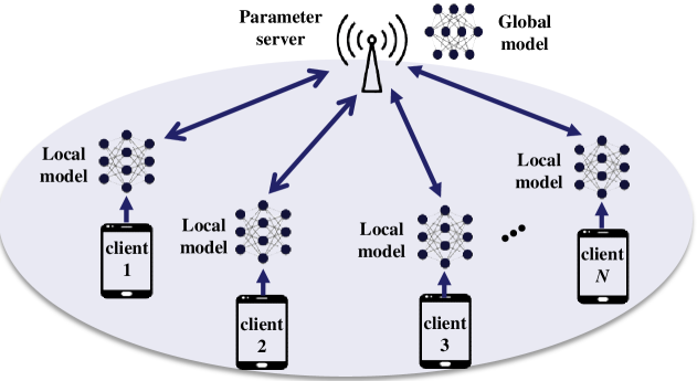
Figure 1: The framework of vanilla FL system.

II-B Differential Privacy

In FL system, the adversary can be “honest-but-curious” server or clients in the system. The adversaries may be curious about a target client’s private data and intend to steal from the shared messages. Furthermore, some clients may collude with the PS to extract private information about a specific client. These attackers can eavesdrop all the shared messages during the execution of the training rather than actively inject false messages into or interrupt message transmissions. The widely used $(\epsilon,\delta)$-DP mechanism for the privacy protection is defined as follows.

Definition 1

($(\epsilon,\delta)$-DP [9]). Suppose that $\cal X$ is a given dataset, and there exist two neighboring datasets $\mathcal{D},\mathcal{D}^{\prime}\subset\mathcal{X}$ such that $|{\cal D}\cup{\cal D^{\prime}}|-|{\cal D}\cap{\cal D^{\prime}}|=1$. A randomized mechanism $\mathcal{M}:\mathcal{X}\rightarrow\mathbb{R}^{d}$ achieves $(\epsilon,\delta)$-DP if for any subset of outputs ${\cal O}\subseteq Range(\mathcal{M})$:

$$\!\!\!\mathbb{P}[\mathcal{M}(\mathcal{D})\in\mathcal{O}]\leq\exp(\epsilon)\cdot\mathbb{P}\left[\mathcal{M}\left(\mathcal{D}^{\prime}\right)\in\mathcal{O}\right]+\delta,$$ (3)

where $\epsilon>0$ and $\delta\in[0,1).$

Note that a smaller $\epsilon$ means stronger privacy protection, and $\delta$ stands for the probability to break the $(\epsilon,0)$-DP. The $(\epsilon,\delta)$-DP can be implemented by properly adding Gaussian noise vector $\bm{\xi}\in{\mathbb{R}}^{d}$ to protect data privacy [9], that is

$$\mathcal{M}(\mathcal{D})={\bm{g}}(\mathcal{D})+\bm{\xi},~{}\,\bm{\xi}\sim\mathcal{N}({\bm{0}},\sigma^{2}{\bf I}_{d}),$$ (4)

where ${\bm{g}}$ is a specified query function, and $\mathcal{N}({\bm{0}},\sigma^{2}{\bf I}_{d})$ is the distribution of a zero-mean Gaussion noise with covariance matrix $\sigma^{2}{\bf I}_{d}$. The required “noise variance” $\sigma^{2}$ (i.e., variance of every element in $\bm{\xi}$) for guaranteeing $(\epsilon,\delta)$-DP in (3) is given by the following lemma.

Lemma 1

[9, Theorem 3.22] Suppose that the randomized mechanism ${\cal M}$ satisfies $(\epsilon,\delta)$-DP defined in (4). Then, the minimum required noise variance $\sigma^{2}$ is given by

$$\sigma^{2}=\frac{2s^{2}\ln(1.25/\delta)}{\epsilon^{2}},$$ (5)

where $s$, the $\ell_{2}$-norm sensitivity of ${\bm{g}}$ in (4), is given by

$$s\triangleq\max_{\mathcal{D},\mathcal{D}^{\prime}\subset{\cal X}}\big{\|}{\bm{g}}(\mathcal{D})-{\bm{g}}\big{(}\mathcal{D}^{\prime}\big{)}\big{\|},$$ (6)

in which ${\cal X}$ is the domain of function ${\bm{g}}$.

Definition 2

(Privacy loss [9]). Suppose that a randomized mechanism $\mathcal{M}$ satisfies $(\epsilon,\delta)$-DP. Let ${\cal D}$ and ${\cal D}^{\prime}$ be two neighboring datasets and ${\bm{o}}$ be a possible random vector of ${\mathcal{M}}(\mathcal{D})$ and ${\mathcal{M}}({\mathcal{D}}^{\prime})$. Then, the privacy loss is defined by

$$c({\bm{o}})=\ln\Big{(}\frac{\mathbb{P}\big{[}{\mathcal{M}}(\mathcal{D})={\bm{o}}\big{]}}{\mathbb{P}\big{[}\mathcal{M}({\mathcal{D}}^{\prime})={\bm{o}}\big{]}}\Big{)}.$$ (7)

Note that when ${\bm{o}}$ is a continuous random vector, $\mathbb{P}[\cdot]$ stands for its probability density function, and this is exactly the case in our work.

III Proposed Privacy-preserving Federated Primal-dual Method

III-A Proposed Primal-dual Method in FL

The federated PDM (FedPDM) solves (2) by successively and iteratively searching for the desired model, a saddle point of the augmented Lagragian (8a), w.r.t. ${\bf x}$, ${\bf x}_{0}$ (minimization) and ${\bm{\lambda}}$ (maximization):

$$\!\!\!\mathcal{L}\big{(}{\bf x},{\bf x}_{0},{\bm{\lambda}}\big{)}=\frac{1}{N}\sum_{i=1}^{N}\mathcal{L}_{i}\big{(}{\bf x}_{i},{\bf x}_{0},{\bm{\lambda}}_{i}\big{)}+h({\bf x}_{0}),$$ (8a)

$$\!\!\!\mathcal{L}_{i}\big{(}{\bf x}_{i},{\bf x}_{0},{\bm{\lambda}}_{i}\big{)}=f_{i}\big{(}{\bf x}_{i}\big{)}+{\bm{\lambda}}_{i}^{\top}({\bf x}_{0}-{\bf x}_{i})+\frac{\rho}{2}\left\|{\bf x}_{0}-{\bf x}_{i}\right\|^{2},$$ (8b)

in which ${\bf x}=[{\bf x}_{1}^{\top},\ldots,{\bf x}_{N}^{\top}]^{\top}$, ${\bm{\lambda}}=[{\bm{\lambda}}_{1}^{\top},\ldots,{\bm{\lambda}}_{N}^{\top}]^{\top}$, $\rho>0$ is the penalty parameter which must be large enough such that ${\cal L}(\cdot)$ is strongly convex in ${\bf x}_{i}$ [51]. Note that, ${\bf x}_{i}$ (primal variable) and ${\bm{\lambda}}_{i}$ (dual variable) are updated at local clients side, while ${\bf x}_{0}$ represents the global model updated at the PS side.

Furthermore, we consider local SGD and partial client participation strategies to improve communication efficiency [3]. Then, the update rule for the proposed FedPDM is as follow,

$${\bf x}_{i}^{t,r+1}= {\bf x}_{i}^{t,r}-\eta^{t}\big{(}\nabla f_{i}({\bf x}_{i}^{t,r};\mathcal{B}_{i}^{t,r})-{\bm{\lambda}}_{i}^{t}+\rho({\bf x}_{i}^{t,r}-{\bf x}_{0}^{t})\big{)},$$ (9a)

$${\bf x}_{i}^{t+1}= {\bf x}_{i}^{t,Q_{i}^{t}},$$ (9b)

$${\bm{\lambda}}_{i}^{t+1}= {\bm{\lambda}}_{i}^{t}+\rho\left({\bf x}_{0}^{t}-{\bf x}_{i}^{t+1}\right),$$ (9c)

$${{\bf y}}_{i}^{t+1}= {\bf x}_{i}^{t+1}-\frac{{\bm{\lambda}}_{i}^{t+1}}{\rho},$$ (9d)

$${\bf x}_{0}^{t+1}= {\rm prox}_{\rho^{-1}h}\Big{(}\frac{1}{K}\sum_{i\in\mathcal{S}_{t}}{{\bf y}}_{i}^{t+1}\Big{)},$$ (9e)

where $\eta^{t}$ denotes the step size; $\mathcal{B}_{i}^{t,r}\subseteq{\cal D}_{i}$ is a mini-batch dataset with $|\mathcal{B}_{i}^{t,r}|=b$; $\mathcal{S}_{t}\subseteq[N]$ denotes the set of participated clients at the $t$-th round with $|\mathcal{S}_{t}|=K$; $Q_{i}^{t}$ represents the number of local SGD iterations (where, rather than a preassigned parameter, $Q_{i}^{t}$ is determined automatically by the algorithm under consideration); $\operatorname{prox}_{\rho^{-1}h}({\bf u})$ is the proximal operator [52] defined by

$$\operatorname{prox}_{\rho^{-1}h}({\bf u})\triangleq\arg\min_{{\bm{x}}}\{h({\bm{x}})+\frac{\rho}{2}\big{\|}{\bm{x}}-{\bf u}\big{\|}^{2}\}.$$ (10)

The proof of (9e) is given in Appendix A. For a preassigned small $\nu>0$ for controlling the size of the vector $({\bf x}_{i}^{t,r+1}-{\bf x}_{i}^{t,r})$, the inner loop ends when

$$\big{\|}\nabla f_{i}({\bf x}_{i}^{t,r};\mathcal{B}_{i}^{t,r})-{\bm{\lambda}}_{i}^{t}+\rho({\bf x}_{i}^{t,r}-{\bf x}_{0}^{t})\big{\|}^{2}\leq\nu,$$ (11)

and $Q_{i}^{t}$ determined by (11) is the smallest number of iterations spent in the inner loop.

Algorithm 1 ​​: DP-FedPDM

1:  Input: System parameters $b$, $T$, $\nu$, $\rho$, $\eta^{t}$, $K.$

2:  Initialize ${\bf x}_{0}^{0}$, $\{{\bf x}_{i}^{0,0}\}$, $\{{\bm{\lambda}}_{i}^{0}\}$, and $\mathcal{S}_{0}=[N]$.

3:  for $t=0,1,\ldots,T-1$ do

4:     Client side:

5:     for $i\in\mathcal{S}_{t}$ in parallel do

6:        Set ${\bf x}_{i}^{t,0}={\bf x}_{0}^{t}$.

7:        for $r=0,1,\ldots$  do

8:           Sample mini-batch $\mathcal{B}_{i}^{t,r}$ from $\mathcal{D}_{i}$.

9:           Update ${\bf x}_{i}^{t,r+1}$ using (9a).

10:           if (11) is satisfied then

11:              Set $Q_{i}^{t}=r+1$ and go to line 13.

12:           end if

13:        end for

14:        Update ${\bf x}_{i}^{t+1}$ by (9b).

15:        Update ${\bm{\lambda}}_{i}^{t+1}$ by (9c).

16:        Update ${\bf y}_{i}^{t+1}$ by (9d).

17:        Compute $\widetilde{{{\bf y}}}_{i}^{t+1}$ by (12) and send it to the PS.

18:     end for

19:     Server side:

20:     Update ${\bf x}_{0}^{t+1}$ by (13).

21:     Update the subset of clients ${\cal S}_{t+1}\subseteq[N]$ through randomly sampling without replacement, and then broadcast ${\bf x}_{0}^{t+1}$ to all the clients.

22:  end for

To guarantee $(\epsilon,\delta)$-DP for the local model ${\bf y}_{i}^{t+1}$ to be uploaded, the aforementioned Gaussian noise $\bm{\xi}_{i}^{t+1}\sim\mathcal{N}\big{(}\bm{0},\sigma_{i,{t+1}}^{2}\mathbf{I}_{d}\big{)}$ is added to ${{\bf y}}_{i}^{t+1}$, i.e.,

$$\widetilde{{{\bf y}}}_{i}^{t+1}={{\bf y}}_{i}^{t+1}+\bm{\xi}_{i}^{t+1}={\bf x}_{i}^{t+1}-\frac{{\bm{\lambda}}_{i}^{t+1}}{\rho}+\bm{\xi}_{i}^{t+1}.$$ (12)

Finally, ${\bf x}_{0}^{t+1}$ given by (9e) can alternatively be expressed as

$${\bf x}_{0}^{t+1}={\rm prox}_{\rho^{-1}h}\Big{(}\frac{1}{K}\sum_{i\in\mathcal{S}_{t}}\widetilde{{{\bf y}}}_{i}^{t+1}\Big{)}.$$ (13)

It is worth noting that the proximal operator is commonly used in optimization algorithms associated with non-differentiable loss functions. For some regularizers, (10) has a closed-form solution. For instance, when $h=\|\cdot\|_{1}$, it leads to a sparse and closed-form solution with soft thresholding operator [52], which can be expressed as follows.

$$\!\big{[}{\rm prox}_{\rho^{-1}h}({\bf x})\big{]}_{i}\!=\!\Bigg{\{}\begin{array}[]{ll}\!\!\!{\rm sgn}([{\bf x}]_{i})\max{\big{\{}\big{|}[{\bf x}]_{i}\big{|}-\frac{1}{\rho},0\big{\}}},\!\!\!\!\!&{{\rm if}\ [x]_{i}\neq 0,\vspace{0.1cm}}\\ \!\!\!0,&{{\rm otherwise.}}\end{array}$$ (16)

where ${\rm sgn}(x)=x/|x|$ for $x\neq 0$. The proposed differentially private FedPDM (DP-FedPDM) is implemented by Algorithm 1.

III-B DP-FedPDM with Bidirectional Model Sparsification

To further reduce the communication cost, by adding artificial model compression operation in the proposed DP-FedPDM, we come up with a bidirectional sparse DP-FedPDM (BSDP-FedPDM). This method transmits sparsified model parameters in both the uplink (clients to the PS) and downlink (PS to clients) communications during each round, while previous works only considered uplink model compressing. Importantly, this approach can also mitigate the adverse effects of DP noise since the variance of DP noise is proportionally to the model size [53]. The $\operatorname{top}_{k}$ or $\operatorname{rand}_{k}$ sparsifiers under consideration are defined as follows:

Definition 3 ($\operatorname{top}_{k}$ and $\operatorname{rand}_{k}$ Sparsifiers [18])

Let ${\bf y}=[y_{1},\dots,y_{d}]^{\top}\in\mathbb{R}^{d}$ and ${\bf y}_{\Downarrow}=[y_{l_{1}},\dots,y_{l_{d}}]^{\top},\,|y_{l_{i}}|\geq|y_{l_{j}}|\ \forall l_{i}\leq l_{j}.$ The $\operatorname{top}_{k}$ and $\operatorname{rand}_{k}$ sparsifier are defined as follows:

$$\operatorname{top}_{k}({\bf y}) \triangleq{\bf y}_{\Downarrow 1:k}=[y_{l_{1}},\dots,y_{l_{k}}]^{\top}\in\mathbb{R}^{k},$$ (17a)

$$\operatorname{rand}_{k}({\bf y}) \triangleq[y_{i_{1}},\dots,y_{i_{k}}]^{\top}\in\mathbb{R}^{k},$$ (17b)

where $\operatorname{rand}_{k}({\bf y})$ is a size-$k$ vector random sample from ${\bf y}$.

For ease of later use, let us define the following notations

$${\bm{I}}(\operatorname{top}_{k}({\bf y})) =[l_{1},\cdots,l_{k}],\ {\cal I}(\operatorname{top}_{k}({\bf y}))=\{l_{1},\cdots,l_{k}\},$$

$${\bm{I}}(\operatorname{rand}_{k}({\bf y})) =[i_{1},\cdots,i_{k}],\ {\cal I}(\operatorname{rand}_{k}({\bf y}))=\{i_{1},\cdots,i_{k}\}.$$

In practice, $\operatorname{rand}_{k}({\bf y})$ may easily omit crucial elements of ${\bf y},$ resulting in performance degradation, especially when $k$ is small. In contrast, $\operatorname{top}_{k}$ preserves components of the top $k$ largest magnitudes, thus maintaining higher model accuracy than $\operatorname{rand}_{k}$. In the following, we present the proposed BSDP-FedPDM with $\operatorname{top}_{k}$ and $\operatorname{rand}_{k}$ sparsifiers, and its pseudo-code is provided in Algorithm 2.

For the $\operatorname{top}_{k}$ scheme at the clients side, the client $i\in\mathcal{S}_{t}$ first performs model sparsification on local model ${\bf y}_{i}^{t+1}$ (cf. (9d)), yielding a sparsified model

$${\widehat{{\bf y}}}_{i}^{t+1}=\operatorname{top}_{k}({\bf y}_{i}^{t+1})\in\mathbb{R}^{k},$$ (19)

and the associated index vector ${\bm{I}}({\widehat{{\bf y}}}_{i}^{t+1})$, implying that the uplink compression ratio $\alpha_{{}_{U}}\triangleq k/d$, i.e., the dimension ratio after and before model sparsification on ${\bf y}_{i}^{t+1}$. Then, a noise vector $(\bm{\xi}_{i}^{t+1})^{\prime}\sim\mathcal{N}\big{(}\bm{0},\sigma_{i,{t+1}}^{2}\mathbf{I}_{k}\big{)}$ is added to ${\widehat{{\bf y}}}_{i}^{t+1}$ for guaranteeing $(\epsilon,\delta)$-DP, that is,

$$(\widehat{{{\bf y}}}_{i}^{t+1})^{\prime}={\widehat{{\bf y}}}_{i}^{t+1}+(\bm{\xi}_{i}^{t+1})^{\prime}.$$ (20)

Next, client $i$ transmits these $k$ index-value pairs $\mathcal{A}_{i}^{t+1}\triangleq({\bm{I}}({\widehat{\bf y}}_{i}^{t+1}),({\widehat{\bf y}}_{i}^{t+1})^{\prime}),\forall i\in\mathcal{S}_{t}$ to the PS. At the PS side, after receiving $\mathcal{A}_{i}^{t+1}$ from client $i$, the PS first converts $(\widehat{{{\bf y}}}_{i}^{t+1})^{\prime}$ into a $d$-dimensional ($d$-dim) vector $({\widehat{\bf y}}_{i}^{t+1})^{\prime\prime}\in\mathbb{R}^{d}$ by zero padding for all the missing entries (line 14). Subsequently, the PS aggregates all the models $({\widehat{\bf y}}_{i}^{t+1})^{\prime\prime},\forall i$ into a complete $d$-dim model, though some zero entries still exist when $|\cup_{i\in{\cal S}_{t}}{\cal I}(\widehat{\bf y}_{i}^{t+1})|<d$. Inspired by [54], we adopt the element-wise aggregation scheme to mitigate the impact of the “curse of primal averaging”. Specifically, (13) is replaced with the following expression:

$$({\bf x}_{0}^{t+1})^{\prime}={\rm prox}_{\rho^{-1}h}\Big{(}\sum_{i\in\mathcal{S}_{t}}({\widehat{\bf y}}_{i}^{t+1})^{\prime\prime}\oslash{\bf w}^{t+1}\Big{)},$$ (21)

where $\oslash$ denotes the element-wise division operator and

$$\!\!\![{\bf w}^{t+1}]_{j}=\Bigg{\{}\begin{array}[]{ll}1,~{}~{}{{\rm if}\ [({\widehat{\bf y}}_{i}^{t+1})^{\prime\prime}]_{j}=0,\vspace{0.1cm}}\\ \sum_{i\in{\cal S}_{t}}\sum_{x\in{\cal I}({\widehat{\bf y}}_{i}^{t+1})}\mathbb{I}_{j}(x),~{}{{\rm otherwise,\vspace{0.1cm}}}\end{array}$$ (24)

in which $\mathbb{I}_{j}(\cdot)$ is the indicator function, defined by

$$\mathbb{I}_{j}(x)=\Bigg{\{}\begin{array}[]{ll}1,&{{\rm if}\ x=j,\vspace{0.1cm}}\\ 0,&{{\rm otherwise.}}\end{array}$$ (27)

To further reduce the communication cost, $\operatorname{top}_{k}$ sparsifier is applied to the global model $({\bf x}_{0}^{t+1})^{\prime}$ by the PS, yielding the sparsified model

$$({\widehat{}{\bf x}_{0}}^{t+1})^{\prime}=\operatorname{top}_{k}(({\bf x}_{0}^{t+1})^{\prime})\in\mathbb{R}^{k^{\prime}},$$ (28)

and the associated index vector ${\bm{I}}(({\widehat{}{\bf x}_{0}}^{t+1})^{\prime})$, and thus the downlink model compression ratio $\alpha_{{}_{D}}=k^{\prime}/d$. Then, the PS broadcasts the index-value pair $\mathcal{A}_{0}^{t+1}={({\bm{I}}(({\widehat{}{\bf x}_{0}}^{t+1})^{\prime}),({\widehat{\bf x}}_{0}^{t+1})^{\prime})}$ to all the selected clients for next round of model update. As the selected clients receive $\mathcal{A}_{0}^{t+1}$, they can recover $\widehat{\bf x}_{0}^{t+1}$ from $({\widehat{\bf x}}_{0}^{t+1})^{\prime}$ through zero padding missing entries. All the other steps remain the same as given in Algorithm 1. The preceding global aggregation and model regulation procedure at the PS also applies to $\operatorname{rand}_{k}$.

Algorithm 2 Proposed BSDP-FedPDM

1:  Input: System parameters $b$, $T$, $\nu$, $\rho$, $\eta^{t}$, $K$, compression ratio $\alpha_{{}_{U}}$ ($\alpha_{{}_{D}}$) for the unplink (downlink).

2:  for $t=0,1,\ldots,T-1$ do

3:     Client side:

4:     Download $\mathcal{A}_{0}^{t}\triangleq({\bm{I}}(({\widehat{}{\bf x}_{0}}^{t})^{\prime}),({\widehat{\bf x}}_{0}^{t})^{\prime})$ from the PS.

5:     Convert $({\widehat{\bf x}}_{0}^{t})^{\prime}$ from dimension $k^{\prime}=d\times\alpha_{{}_{D}}$ into the associated $d$-dim $\widehat{\bf x}_{0}^{t}$ with $\|\widehat{\bf x}_{0}^{t}\|_{0}=k^{\prime}$.

6:     for $i\in\mathcal{S}_{t}$ in parallel do

7:        Set ${\bf x}_{i}^{t,0}=\widehat{{\bf x}}_{0}^{t}$.

8:        Obtain ${\bf y}_{i}^{t+1}$ by following lines 7–16 in Algorithm 1.

9:        Update ${\widehat{{\bf y}}}_{i}^{t+1}$ by (19).

10:        Compute $(\widehat{{{\bf y}}}_{i}^{t+1})^{\prime}$ by (20) for $k=d\times\alpha_{{}_{U}}$.

11:        Send the $\mathcal{A}_{i}^{t+1}=({\bm{I}}({\widehat{{\bf y}}}_{i}^{t+1}),({\widehat{\bf y}}_{i}^{t+1})^{\prime})$ to the PS.

12:     end for

13:     Server side:

14:     Convert $({\widehat{\bf y}}_{i}^{t+1})^{\prime},\forall i\in\mathcal{S}_{t}$ from dimension $k=d\times\alpha_{{}_{U}}$ into the associated $d$-dim $(\widehat{\bf y}_{0}^{t+1})^{\prime\prime}$ with $\|({\widehat{\bf y}}_{i}^{t+1})^{\prime\prime}\|_{0}$$=$$k$.

15:     Obtain $({\bf x}_{0}^{t+1})^{\prime}$ by (21).

16:     Obtain $({\widehat{}{\bf x}_{0}}^{t+1})^{\prime}$ by (28) with dimension $k^{\prime}=d\times\alpha_{{}_{D}}$.

17:     Update the subset of clients ${\cal S}_{t+1}\subseteq[N]$ through randomly sampling without replacement.

18:     Broadcast $\mathcal{A}_{0}^{t+1}=({\bm{I}}(({\widehat{}{\bf x}_{0}}^{t+1})^{\prime}),({\widehat{\bf x}}_{0}^{t+1})^{\prime})$ to all selected clients.

19:  end for

Let us conclude this section with the following properties of the proposed BSDP-FedPDM:

• In view of model dimension reduction resulted from the sparsifier applied, the term inside the parentheses of (21) (for global model aggregation and regularization) can be thought of as an actuarial average of each non-zero element (a true model element) of $({\widehat{\bf y}}_{i}^{t+1})^{\prime\prime},\forall i\in{\cal S}_{t}$, thereby free from the effect of “curse of primal averaging”.

• Uplink communication cost can be reduced by 50% when $\alpha_{{}_{U}}=1$ (i.e., without sparsification) owing to the combined model $(\widehat{{{\bf y}}}_{i}^{t+1})^{\prime}$ perturbed by DP noise (cf. (12)), instead of $({\bf x}_{i}^{t+1},{\bm{\lambda}}_{i}^{t+1})$, while the total communication cost will be reduced to $50\%\times\alpha_{{}_{U}}$ if model sparsification under the control of the system operator is applied, i.e., $\alpha_{{}_{U}}<1$. However, as a tradeoff with communication cost reduction, the model sparsification will also induce some performance loss.

• The global aggregation and model regularization is performed by the PS (cf. (13) and (21)). When the non-smooth $\ell_{1}$-norm regularizer (i.e., $h({\bf x})=\gamma\|{\bf x}\|_{1}$ where $\gamma$ is a non-negative parameter) is used, the trained global model ${\bf x}^{\star}$ (like an optimization based sparsity promoter rather than dimension reduction by a sparsifier) will be a sparse solution, thus especially suited to the $\operatorname{top}_{k}$ sparsification scheme for larger communication cost saving. Furthermore, we found that the performance of ${\bf x}^{\star}$ is robust against the DP noise, which will be justified by the experimental results in Subsections V-D1 and V-D4 later.

• The property (P3) also applies to DP-FedPDM simply because the proposed BSDP-FedPDM and DP-FedPDM are identical as $\alpha_{{}_{U}}=\alpha_{{}_{D}}=1$.

IV Privacy and Convergence Analysis for DP-FedPDM

IV-A Assumptions

Assumption 1 (Smoothness and lower bounded)

Each loss function $f_{i}(\cdot)$ in (2) is $L$-smooth, i.e., $f_{i}$ is continuously differentiable and there exists an $L>0$ such that

$$\|\nabla f_{i}({\bm{x}})-\nabla f_{i}({\bm{y}})\big{\|}\leq L\big{\|}{\bm{x}}-{\bm{y}}\big{\|},\forall i\in[N].$$ (29)

Besides, $\mathcal{L}(\cdot)$ given in (8a) is bounded below, i.e.,

$$\underline{f}\triangleq\inf_{{\bf x},{\bf x}_{0},{\bm{\lambda}}}\mathcal{L}({\bf x},{\bf x}_{0},{\bm{\lambda}})>-\infty.$$ (30)

Assumption 2 (Unbiased gradient and bounded variance)

For the mini-batch dataset $\mathcal{B}_{i}^{t,r}$ with size $b$ at the $t$-th round, the associated mini-batch gradient satisfies

$$\mathbb{E}\left[\nabla f_{i}\big{(}{\bf x}_{i}^{t,r};\mathcal{B}_{i}^{t,r}\big{)}\right]=\nabla f_{i}\big{(}{\bf x}_{i}^{t,r}\big{)},$$ (31a)

$$\mathbb{E}\Big{[}\big{\|}\nabla f_{i}\big{(}{\bf x}_{i}^{t,r};\mathcal{B}_{i}^{t,r}\big{)}-\nabla f_{i}({\bf x}_{i}^{t,r})\big{\|}^{2}\Big{]}\leq{\phi^{2}},$$ (31b)

for all $t,r\leq Q_{i}^{t}$, where $Q_{i}^{t}$ is yielded by Algorithm 1, and the upper bound $\phi^{2}\to 0$ as $b\to|\mathcal{D}_{i}|$ [27].

Assumption 3 (Bounded gradient)

The mini-batch gradients $\nabla f_{i}({\bf x}_{i}^{t,r};\mathcal{B}_{i}^{t,r})$, $\forall t,r$, are bounded, that is,

$$\|\nabla f_{i}({\bf x}_{i}^{t,r};\mathcal{B}_{i}^{t,r})\|\leq G.$$ (32)

IV-B Privacy Analysis

Theorem 1

With the noise vector $\bm{\xi}_{i}^{t}\sim\mathcal{N}\big{(}\bm{0},\sigma_{i,t}^{2}\mathbf{I}_{d}\big{)}$ added to ${\bf y}_{i}^{t}$ (cf. (12)), the minimum noise variance $\sigma_{i,t}^{2}$ for guaranteeing $(\epsilon,\delta)$-DP is given by

$$\sigma_{i,t}^{2}=\frac{2s_{i,t}^{2}\ln\big{(}1.25/\delta\big{)}}{\epsilon^{2}},$$ (33)

where

$$s_{i,t}=\Bigg{\{}\begin{array}[]{ll}\text{{\normalsize$\frac{1-|1-\rho\eta^{t}|^{Q_{i}^{t}}}{1-|1-\rho\eta^{t}|}$}}4\eta^{t}G,&{{\rm if}\ \rho\eta^{t}\neq 2,\vspace{0.1cm}}\\ 4\eta^{t}Q_{i}^{t}G,&{{\rm otherwise.}}\end{array}$$ (36)

Proof: The (36) can be derived from the definition of $\ell_{2}$-sensitivity of ${\bf y}_{i}^{t}$ [9]. The proof is given in Appendix A. $\hfill\blacksquare$

Theorem 1 shows that $\sigma_{i,t}^{2}$ is larger for larger $Q_{i}^{t}$, though a larger $Q_{i}^{t}$ can improve the communication efficiency [6]. Hence, the value of $Q_{i}^{t}$ (yielded by Algorithm 1) determines the tradeoff between privacy protection and communication efficiency.

The total privacy loss of client $i$ yielded by Algorithm 1, which is the sum of all the privacy losses (cf. (7)) over $T$ communication rounds [9], it can be estimated by multiple methods, e.g., the moments accountant method [53], which is used in proving the following theorem.

Theorem 2

Let $p_{i}=K/N$ and $q_{i}=Q_{i}^{t}b/m_{i}$, that are the fraction of participating clients and data used by client $i$, respectively. Under the $(\epsilon,\delta)$-DP at each round for client $i$, the minimum total privacy loss over $T$ communication rounds is given by

$$\bar{\epsilon}_{i}^{T} =c_{0}q_{i}^{2}\epsilon\sqrt{\frac{p_{i}T}{1-q_{i}}},\forall i\in[N],$$ (37)

where $c_{0}>0$ is a constant dependent upon $\delta$.

Proof: The proof basically follows that of Theorem 1 reported in [6] for the case of data sampling without replacement. $\blacksquare$

Theorem 2 shows how the mechanisms of client sampling and data sampling impact the total privacy loss $\bar{\epsilon}_{i}^{T},\forall i$. The larger value of $\bar{\epsilon}_{i}^{T}$, the larger value of $\epsilon$ by (37), implying weaker privacy protection but better learning performance. This will be justified in our experimental results later.

IV-C Convergence Analysis

Motivated by [21], the quantity $P(\{{\bf x}_{i}^{t}\},{\bf x}_{0}^{t},\{{\bm{\lambda}}_{i}^{t}\})$ used as convergence performance measure is defined by

$$P(\{{\bf x}_{i}^{t}\},{\bf x}_{0}^{t},\{{\bm{\lambda}}_{i}^{t}\})\triangleq \sum_{j=1}^{N}\Big{[}\big{\|}\nabla_{{\bf x}_{j}}\mathcal{L}(\{{\bf x}_{i}^{t}\},{\bf x}_{0}^{t},\{{\bm{\lambda}}_{i}^{t}\})\big{\|}^{2}$$

$$~{}~{}+\big{\|}\nabla_{{\bm{\lambda}}_{j}}\mathcal{L}(\{{\bf x}_{i}^{t}\},{\bf x}_{0}^{t},\{{\bm{\lambda}}_{i}^{t}\})\big{\|}^{2}\Big{]}+\big{\|}\nabla_{{\bf x}_{0}}\mathcal{L}(\{{\bf x}_{i}^{t}\},{\bf x}_{0}^{t},\{{\bm{\lambda}}_{i}^{t}\})\big{\|}^{2}.$$ (38)

It can be verified that if $P(\{{\bf x}_{i}^{t}\},{\bf x}_{0}^{t},\{{\bm{\lambda}}_{i}^{t}\})\rightarrow 0$ as $t$ increases, then a stationary-point solution to problem (2) can be obtained [27].

Theorem 3

Suppose that Assumptions 1-3 hold and $2\sqrt{5}-4\leq L\leq\rho/4$. Then, the following inequality holds:

$$\frac{1}{T}\sum_{t=0}^{T-1}\mathbb{E}\big{[}P(\{{\bf x}_{i}^{t}\},{\bf x}_{0}^{t},\{{\bm{\lambda}}_{i}^{t}\})\big{]}\leq\zeta\triangleq\underbrace{\frac{(\mathcal{L}(\{{\bf x}_{i}^{0}\},{\bf x}_{0}^{0},\{{\bm{\lambda}}_{i}^{0}\})-\underline{f})C_{0}}{T}}_{A_{0}}+\underbrace{C_{1}\nu}_{A_{1}}+\underbrace{C_{2}\phi^{2}}_{A_{2}}+\underbrace{C_{3}\sigma^{2}}_{A_{3}},$$ (39)

where $\nu$, $\phi^{2}$ have been defined in (11) and Assumption 2, respectively; $\sigma^{2}\triangleq\max_{i,t}\sigma_{i,t}^{2};$ $C_{0},$ $C_{1},$ $C_{2},$ $C_{3}$ are constants depending on system parameters $\rho$ and $L$ given in (C.5).

Proof: The proof is given in Appendix B. $\hfill\blacksquare$

Let us conclude this section with the following two remarks based on Theorem 1 and Theorem 3.

Remark 1

The convergence performance bound in Theorem 3 is dependent upon $A_{0}$, $A_{1}$, $A_{2}$, $A_{3}$. Specifically, i) $A_{0}\rightarrow 0$ as $T$ increases; ii) $A_{1}\rightarrow 0$ as $\nu\rightarrow 0$; iii) $A_{2}$ can be made arbitrarily small for $b$ large enough since $\phi^{2}\rightarrow 0$ as $b\rightarrow|{\cal D}_{i}|$ by (31b); iv) $A_{3}$ can be reduced by letting $\rho\eta^{t}\rightarrow 1$ or increasing $\epsilon$ by Theorem 1.

Remark 2

(Communication complexity). By Theorem 3, to achieve a $\zeta$-stationary solution under the following parameter setting:

$$T =4(\mathcal{L}(\{{\bf x}_{i}^{0}\},{\bf x}_{0}^{0},\{{\bm{\lambda}}_{i}^{0}\})-\underline{f})C_{0}/\zeta,$$ (40a)

$$\nu =\zeta/(4C_{1}),\phi^{2}=\zeta/(4C_{2}),\sigma^{2}=\zeta/(4C_{3}),$$ (40b)

where $\sigma^{2}\triangleq\max_{i,t}\sigma_{i,t}^{2}$. It can be inferred that (40b) can be achieved by Remark 1. Finally, we would like to emphasize that the required $T$ is in $\mathcal{O}(1/\zeta)$ by (40a), while to the best of our knowledge, most of state-of-the-art FL algorithms can only attain $T$ in ${\cal O}(1/\zeta^{2})$ for non-convex problems [55, 56].

V Experimental Results and Discussions

V-A Experimental Model

We evaluate the performance of the proposed DP-FedPDM by considering the commonly known non-convex and non-smooth logistic regression problem [27] with the loss function

$$F({\bf X})=\frac{1}{N}\sum_{i=1}^{N}f_{i}({\bf X})+\gamma\|{\bf X}\|_{1},$$ (41)

where $\|{\bf X}\|_{1}$ $=\sum_{j=1}^{m}\sum_{k=1}^{n}\left|[{\bf X}]_{jk}\right|$, ${\bf X}=[{\bm{x}}_{1},\dots,{\bm{x}}_{m}]^{\top}\in\mathbb{R}^{m\times n}$, and $\gamma>0$ denotes the regularization parameter, and

$$f_{i}({\bf X})=\frac{1}{|{\cal D}_{i}|}\sum_{j=1}^{|{\cal D}_{i}|}\Big{[}\ln\big{(}1+\exp(-{\rm Tr}({\bf X}{\bf Y}_{ij})\big{)}\Big{]}+\beta\sum_{j,k}\frac{[{\bf X}]_{jk}^{2}}{1+[{\bf X}]_{jk}^{2}},$$ (42)

in which ${\bf Y}_{ij}={\bm{a}}_{ij}{\bm{b}}_{ij}^{\top}$ is sparse, since ${\bm{a}}_{ij}\in\mathbb{R}^{n}$ represents the feature vector and ${\bm{b}}_{ij}\in\mathbb{R}^{m}$ satisfying $\|{\bm{b}}_{ij}\|_{0}=1$ denotes the label vector of the $j$-th sample in $\mathcal{D}_{i}$. The concavity of $f_{i}$ increases as $\beta$ increases. Note that the regularizer $\|{\bf X}\|_{1}$ (convex envelope of $\|{\bf X}\|_{0}$ [51]) is non-smooth for the trained model ${\bf X}^{\star}$ to be sparse. It is worth mentioning that the $k$-th row of ${\bf X}^{\star}$ (i.e., $({\bm{x}}_{k}^{\star})^{\top}$) corresponds to the centroid of the $k$-th true class among $m$ true classes.

In the testing stage, for the given feature vector, denoted as $\bm{a}^{\prime}\in{\mathbb{R}}^{n}$, of an unknown class (whose true class number is given by $k^{\prime}=\arg\max_{k}\{b_{k}^{\prime},k\in[m]\}$), where $b_{k}^{\prime}$ is the $k$-th element of the true label vector ${\bm{b}}^{\prime}\in{\mathbb{R}}^{m}$. We compute the following softmax function [6]

$$z_{k}=\frac{\exp({{\bm{x}}_{k}^{\top}\bm{a}^{\prime}})}{\sum_{j=1}^{m}\exp({{\bm{x}}_{j}^{\top}\bm{a}^{\prime}})},\forall k\in[m].$$ (43)

Then the correct decision is made if $\arg\max_{k}\{z_{k}\}=k^{\prime}$. Finally, the overall testing accuracy is obtained as the correct classification rate over the testing dataset.

V-B Datasets and Benchmark Algorithms

V-B1 Datasets

Two benchmark datasets, Adult [57] and MNIST [58], are considered for performance evaluation. The MNIST dataset consists of 60,000 training samples and 10,000 testing samples, while the Adult dataset consists of 32,561 training samples and 16,281 testing samples. To simulate the FL system, we distribute all training samples across $N=100$ clients in a non-identical and independently distributed (non-i.i.d.) manner, ensuring each client possessed partial labels for the data.

• For MNIST dataset for which $(m,n)=(10,785)$, we followed the heterogeneous data partition method in [3], where each client is allocated data samples of only four labels with $|{\cal D}_{i}|=600$. This leads to a high degree of non-i.i.d. datasets among clients.

• For Adult dataset for which $(m,n)=(2,81)$, following [5], all the training samples are uniformly distributed among total $N=100$ clients such that each client only contains data from one class with $|{\cal D}_{i}|=325$.

V-B2 Benchmark Algorithms

Some state-of-the-art algorithms, including FedAvg [5], SCAFFOLD [26], FedProx [41] and FedDyn [43], are tested for performance comparison with the proposed algorithms.

V-C Parameter Setting

For all our experiments, we maintained the following parameter settings: $K=30$, $b=10$, $\rho=10$, $\delta=10^{-4}$, $\nu=10^{-2}$, $\beta=0.5$, and $\gamma=0.5$. The choice of the learning rate $\eta^{t}$ depends on the dataset under consideration. For MNIST dataset, the local learning rate is set as $\eta^{t}=0.04/\sqrt{1+t}$, while for Adult dataset, the local learning rate is adjusted to $\eta^{t}=0.01/\sqrt{1+t}$. For client $i$, the value of $\epsilon$ used at each each communication round is set according to (37) (cf. Theorem 2), provided that the total privacy loss $\bar{\epsilon}_{i}^{T},\forall i$ is preassigned. The above system parameters are also the default values used for the experiment, otherwise, they will be clearly specified instead.

V-D Experiment Results

Each experiment is conducted using five different randomly generated initial points. The uplink communication cost refers to the size of the data transmitted from all participated clients to the PS over the entire training process, which is calculated by $32k\times T\times K$ bits [18] assuming 32 bits for every real number. Next, let us present the performance of the proposed algorithms under various experimental settings.

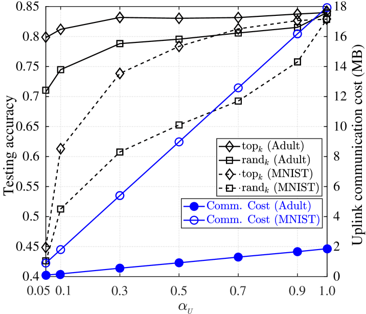
Figure 2: Testing accuracy and uplink communication costs of the proposed BSDP-FedPDM for $\alpha_{{}_{U}}\in\{0.05,0.1,0.3,0.5,0.7,0.9,1\}$ and $\alpha_{{}_{D}}=1$.

Figure 3: Testing accuracy of the proposed BSDP-FedPDM for $\alpha_{{}_{D}}\in\{0.5,0.75,0.9,1\}$ and $\alpha_{{}_{U}}=0.5$.

V-D1 Impact of model sparsification

We first evaluate the performance (testing accuracy) of the BSDP-FedPDM algorithm for different uplink and downlink compression ratios. In this experiment, we set $T=200$, $\bar{\epsilon}_{i}^{T}=0.5$ for the Adult dataset and $\bar{\epsilon}_{i}^{T}=20$ for MNIST dataset. As shown in Fig. 2, reducing $\alpha_{{}_{U}}$ brings savings in communication cost (i.e., higher communication efficiency) along with some performance loss, which is consistent with the property (P2) of the proposed algorithm. The performance loss of the proposed BSDP-FedPDM is less sensitive to $\alpha_{{}_{U}}$ for Adult dataset with $m=2$ than for MNIST dataset with $m=10$. Moreover, the $\operatorname{top}_{k}$ sparsifier exhibits superior performance over $\operatorname{rand}_{k}$ sparsifier, especially with significant performance gap for MNIST dataset.

Figure 3 illustrates the impact of downlink compression ratio on the performance of BSDP-FedPDM. Notably, MNIST dataset is more sensitive to downlink model compression than Adult dataset. However, we would like to emphasize if the tradeoff between the communication cost (larger for larger compression ratio) and the performance (better for larger compression ratio) is application-dependent and/or data-dependent, and controlled by the system operator through the choice of $(\alpha_{{}_{U}},\alpha_{{}_{D}})$.

V-D2 Impact of DP

Figure 4 shows the experimental results (testing accuracy versus communication round) for the proposed DP-FedPDM for different total privacy loss $\bar{\epsilon}_{i}^{T}$. One can observe that DP-FedPDM performs better for larger $\bar{\epsilon}_{i}^{T}$ (or weaker privacy protection) with the best performance for the case “without DP” (no privacy protection), and that its the testing accuracy increases with communication round, thus exhibiting the convergence behavior w.r.t. communication round. These results are consistent with our analyses (cf. Theorems 2 and 3 and Remark 1).

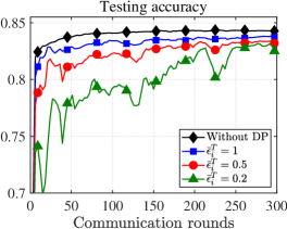
(a)

(b)

Figure 4: Performance of the proposed DP-FedPDM on (a) Adult dataset for the cases of “without DP”, $\bar{\epsilon}_{i}^{T}\in\{0.2,0.5,1\}$ and (b) MNIST dataset for the cases of “without DP”, $\bar{\epsilon}_{i}^{T}\in\{10,20,30\}$.

V-D3 Impact of non-convex loss function

Figure 5 presents the performance of DP-FedPDM for $\beta\in\{0,0.05,0.5,5\}$ while maintaining $\bar{\epsilon}_{i}^{T}=0.5$ for Adult dataset and $\bar{\epsilon}_{i}^{T}=20$ for MNIST dataset. It can be observed that the smaller the $\beta$, the better its performance simply because the convexity of the loss function $f_{i}$ used by client $i$ increases with $\beta$ (cf. (42)), implying that the non-convexity of $f_{i}$ is always a concern in FL system.

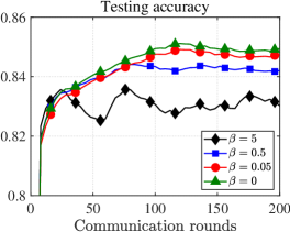
(a)

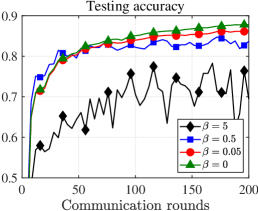
(b)

Figure 5: Performance of DP-FedPDM for $\beta\in\{0,0.05,0.5,5\}$ for (a) Adult dataset, where $\bar{\epsilon}_{i}^{T}=0.5$, and (b) MNIST dataset, where $\bar{\epsilon}_{i}^{T}=20$.

V-D4 Impact of non-smooth regularizer

Figure 6 illustrates the testing accuracy versus communication round achieved by DP-FedPDM for $\gamma=\{0,0.05,0.5,5\}$. It can be observed from this figure, that the testing accuracy performance is better for the withtout DP (w/o DP) case than for the case with DP (w/ DP), thus consistent with the widely known fact about the tradeoff between the performance and the privacy protection. Another observation is that the testing accuracy performance for the w/o DP case as shown Figs. 6(a) and 6(c) (the case with DP as shown in Figs. 6(b) and 6(d)) is better for smaller (larger) $\gamma$, meanwhile demonstrating that the performance with a suitable $\gamma$ value is robust against DP noise, which is consistent with the properties (P3) and (P4).

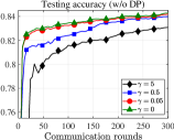
(a)

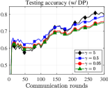
(b)

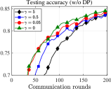
(c)

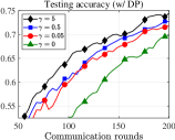
(d)

Figure 6: Performance of the proposed DP-FedPDM for the cases of $\gamma\in\{0,0.05,0.5,5\}$ for (a) without DP and (b) $\bar{\epsilon}_{i}^{T}=0.1$ for Adult dataset, and (c) without DP and (d) $\bar{\epsilon}_{i}^{T}=5$ for MNIST dataset.

(a)

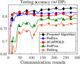
(b)

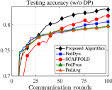
(c)

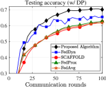
(d)

Figure 7: Performance comparison between the proposed DP-FedPDM without model sparsification and benchmark algorithms for the cases of (a) “without DP” and (b) $\bar{\epsilon}_{i}^{T}=0.5$ for Adult dataset; and the cases of (c) “without DP” and (d) $\bar{\epsilon}_{i}^{T}=10$ for the MNIST dataset.

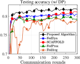
(a)

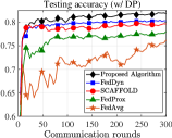
(b)

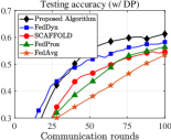
(c)

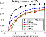
(d)

Figure 8: Performance comparison between the proposed BSDP-FedPDM and benchmark algorithms for the cases of (a) $(\alpha_{{}_{U}},\alpha_{{}_{D}})=(0.1,1)$, and (b) $(\alpha_{{}_{U}},\alpha_{{}_{D}})=(0.5,0.75)$ with $\bar{\epsilon}_{i}^{T}=0.5$ for Adult dataset; and the cases of (c) $(\alpha_{{}_{U}},\alpha_{{}_{D}})=(0.1,1)$, and (d) $(\alpha_{{}_{U}},\alpha_{{}_{D}})=(0.5,0.75)$ with $\bar{\epsilon}_{i}^{T}=20$ for MNIST dataset.

V-D5 Performance comparison with benchmark algorithms

Figure 7 (Figure 8) show some comparison results versus without (with) model sparsification for the proposed DP-FedPDM (BSDP-FedPDM) and the above-mentioned four benchmark algorithms. One can see from Fig. 7, all the algorithms under test incur some performance loss when DP is applied. Nevertheless, we can conclude that DP-FedPDM outperforms all the other algorithms under test for both with DP and w/o DP cases, in addition to its stronger robustness against the DP noise, as stated in the property (P3). Moreover, the same observations from Fig. 7 also apply to Fig. 8. Therefore, the above conclusions for DP-FedPDM are also true for BSDP-FedPDM.

VI Conclusions

We have presented two DP based primal-dual FL algorithms for solving a problem with a non-convex loss function plus a non-smooth regularizer, including DP-FedPDM (without model sparsification) and BSDP-FedPDM (with model sparsification considered) together with their intriguing insightful properties (cf. (P1) through (P4) at the end of Section III-B), also suggesting that the $\operatorname{top}_{k}$ sparsifier and $\ell_{1}$-norm regularizer is a great match for better learning performance and lower communication cost. Note that DP-FedPDM is actually a special case of BSDP-FedPDM when $\alpha_{{}_{U}}=\alpha_{{}_{D}}=1$. Moreover, we also presented the privacy and convergence analyses for the proposed DP-FedPDM (cf. Theorems 2 and 3, Remarks 1 and 2), that can be used as guidelines for the FL algorithm design, especially, the tradeoff between the testing performance and privacy protection level. Extensive experimental results on non-i.i.d. real-world data over all the clients under the practical classification scenario have been provided to demonstrate their efficacy, properties, and analytical results, and much superior performance over some state-of-the-art algorithms.

Appendix A Proof of (13)

According to (9e), we have

$${\bf x}_{0}^{t+1}= \arg\min\limits_{{\bf x}_{0}}\mathcal{L}\big{(}{\bf x}^{t+1},{\bf x}_{0},{\bm{\lambda}}^{t+1}\big{)}$$

$$\overset{(a)}{=} \arg\min\limits_{{\bf x}_{0}}h({\bf x}_{0})+\sum_{i=1}^{N}\left(\langle{\bm{\lambda}}_{i}^{t+1},{\bf x}_{0}-{\bf x}_{i}^{t+1}\rangle+\frac{\rho}{2}\left\|{\bf x}_{0}-{\bf x}_{i}^{t+1}\right\|^{2}\right)$$

$$\overset{(b)}{=} \arg\min\limits_{{\bf x}_{0}}h({\bf x}_{0})+\frac{\rho}{2}\sum_{i=1}^{N}\Big{(}\big{\|}\frac{1}{\rho}{\bm{\lambda}}_{i}^{t+1}\big{\|}^{2}+2\big{\langle}\frac{1}{\rho}{\bm{\lambda}}_{i}^{t+1},{\bf x}_{0}^{t}-{\bf x}_{i}^{t+1}\big{\rangle}+\left\|{\bf x}_{0}-{\bf x}_{i}^{t+1}\right\|^{2}\Big{)}$$

$$= \arg\min\limits_{{\bf x}_{0}}h({\bf x}_{0})+\frac{\rho}{2}\sum_{i=1}^{N}\left(\big{\|}{\bf x}_{0}-({\bf x}_{i}^{t+1}-\frac{1}{\rho}{\bm{\lambda}}_{i}^{t+1})\big{\|}^{2}\right)$$

$$\overset{(c)}{=} \arg\min\limits_{{\bf x}_{0}}h({\bf x}_{0})+\frac{\rho}{2}\big{\|}{\bf x}_{0}-\frac{1}{N}\sum_{i=1}^{N}({\bf x}_{i}^{t+1}-\frac{1}{\rho}{\bm{\lambda}}_{i}^{t+1})\big{\|}^{2}$$

$$\overset{}{=} {\rm prox}_{\rho^{-1}h}\Big{(}\frac{1}{N}\sum_{i=1}^{N}({\bf x}_{i}^{t+1}-\frac{1}{\rho}{\bm{\lambda}}_{i}^{t+1})\Big{)},$$ (A.1)

where $(a)$, $(b)$ and $(c)$ hold because $f_{i}({\bf x}_{i})$, ${\bf x}_{i}$, ${\bm{\lambda}}_{i},\,\forall i$ are constants w.r.t. ${\bf x}_{0}$. $\hfill\blacksquare$

Appendix B Proof of Theorem 2

Suppose that $\mathcal{D}_{i}$ and $\mathcal{D}_{i}^{\prime}$ are the neighboring datasets that differ in only one data sample. For clarity of the following proof, we introduce the notations ${\bf x}_{i,\mathcal{D}_{i}}$ and ${\bf x}_{i,\mathcal{D}_{i}^{\prime}}$ to represent the updated values of ${\bf x}_{i}$, derived from the datasets $\mathcal{D}_{i}$ and $\mathcal{D}_{i}^{\prime}$, respectively. Similarly, we define ${\bm{\lambda}}_{i,\mathcal{D}_{i}}$ and ${\bm{\lambda}}_{i,\mathcal{D}_{i}^{\prime}}$ as the updated values of ${\bm{\lambda}}_{i}$ from the datasets $\mathcal{D}_{i}$ and $\mathcal{D}_{i}^{\prime}$. Let ${\rm spar}(\cdot)$ denote the sparsifier. According to (6), the sensitivity of ${\rm spar}({\bf y}_{i}^{t+1})$ is given as follows,

$$s_{i,t}= \max_{\mathcal{D}_{i},\mathcal{D}_{i}^{\prime}}\big{\|}{\rm spar}({\bf y}_{i,\mathcal{D}_{i}}^{t+1}-{\bf y}_{i,\mathcal{D}_{i}^{\prime}}^{t+1})\big{\|}$$

$$\leq \max_{\mathcal{D}_{i},\mathcal{D}_{i}^{\prime}}\big{\|}{\bf y}_{i,\mathcal{D}_{i}}^{t+1}-{\bf y}_{i,\mathcal{D}_{i}^{\prime}}^{t+1}\big{\|}$$

$$= \max_{\mathcal{D}_{i},\mathcal{D}_{i}^{\prime}}\big{\|}{\bf x}_{i,\mathcal{D}_{i}}^{t+1}-{\bf x}_{i,\mathcal{D}_{i}^{\prime}}^{t+1}-\frac{1}{\rho}\big{(}{\bm{\lambda}}_{i,\mathcal{D}_{i}}^{t+1}-{\bm{\lambda}}_{i,\mathcal{D}_{i}^{\prime}}^{t+1}\big{)}\big{\|}$$

$$\overset{(a)}{=} \max_{\mathcal{D}_{i},\mathcal{D}_{i}^{\prime}}\big{\|}{\bf x}_{i,\mathcal{D}_{i}}^{t+1}-{\bf x}_{i,\mathcal{D}_{i}^{\prime}}^{t+1}-\frac{1}{\rho}\big{(}{\bm{\lambda}}_{i}^{t}-{\bm{\lambda}}_{i}^{t}\big{)}+{\bf x}_{i,\mathcal{D}_{i}}^{t+1}-{\bf x}_{i,\mathcal{D}_{i}^{\prime}}^{t+1}+\big{(}{\bf x}_{0}^{t}-{\bf x}_{0}^{t}\big{)}\big{\|}$$

$$= 2\max_{\mathcal{D}_{i},\mathcal{D}_{i}^{\prime}}\big{\|}{\bf x}_{i,\mathcal{D}_{i}}^{t+1}-{\bf x}_{i,\mathcal{D}_{i}^{\prime}}^{t+1}\big{\|},$$ (B.1)

where $(a)$ holds true due to ${\bm{\lambda}}_{i}^{t}={\bm{\lambda}}_{i}^{t-1}-\rho\big{(}{\bf x}_{i}^{t}-{\bf x}_{0}^{t}\big{)}$ in (9c). By combining (9) and (B), we have

$$\big{\|}{\bf x}_{i,\mathcal{D}_{i}}^{t+1}-{\bf x}_{i,\mathcal{D}_{i}^{\prime}}^{t+1}\big{\|}=\big{\|}{\bf x}_{i,\mathcal{D}_{i}}^{t,Q_{i}^{t}}-{\bf x}_{i,\mathcal{D}_{i}^{\prime}}^{t,Q_{i}^{t}}\big{\|}$$

$$= \Big{\|}\big{(}{\bf x}_{i,\mathcal{D}_{i}}^{t,Q_{i}^{t}-1}-\eta^{t}(\nabla f_{i}({\bf x}_{i,\mathcal{D}_{i}}^{t,Q_{i}^{t}};{\mathcal{B}}_{i}^{t})-{\bm{\lambda}}_{i}^{t}+\rho({\bf x}_{i,\mathcal{D}_{i}}^{t,Q_{i}^{t}-1}-{\bf x}_{0}^{t}))\big{)}$$

$$-\big{(}{\bf x}_{i,\mathcal{D}_{i}^{\prime}}^{t,Q_{i}^{t}-1}-\eta^{t}(\nabla f_{i}({\bf x}_{i,\mathcal{D}_{i}^{\prime}}^{t,Q_{i}^{t}};({{\mathcal{B}}_{i}^{t}})^{\prime})-{\bm{\lambda}}_{i}^{t}+\rho({\bf x}_{i,\mathcal{D}_{i}^{\prime}}^{t,Q_{i}^{t}-1}-{\bf x}_{0}^{t}))\big{)}\Big{\|}$$

$$\overset{(a)}{\leq} \big{|}1-\rho\eta^{t}\big{|}\big{\|}{\bf x}_{i,\mathcal{D}_{i}}^{t,Q_{i}^{t}-1}-{\bf x}_{i,\mathcal{D}_{i}^{\prime}}^{t,Q_{i}^{t}-1}\big{\|}+\eta^{t}\big{\|}\nabla f_{i}({\bf x}_{i,\mathcal{D}_{i}}^{t,Q_{i}^{t}};{\mathcal{B}}_{i}^{t})-\nabla f_{i}({\bf x}_{i,\mathcal{D}_{i}^{\prime}}^{t,Q_{i}^{t}};({{\mathcal{B}}_{i}^{t}})^{\prime})\big{\|}$$

$$\overset{(b)}{\leq} \big{|}1-\rho\eta^{t}\big{|}^{2}\big{\|}{\bf x}_{i,\mathcal{D}_{i}}^{t,Q_{i}^{t}-2}-{\bf x}_{i,\mathcal{D}_{i}^{\prime}}^{t,Q_{i}^{t}-2}\big{\|}+2\eta^{t}G(1+\big{|}1-\rho\eta^{t}\big{|})$$

$$\vdots$$

$$\leq \big{|}1-\rho\eta^{t}\big{|}^{Q_{i}^{t}}\big{\|}{\bf x}_{i,\mathcal{D}_{i}}^{t,0}-{\bf x}_{i,\mathcal{D}_{i}^{\prime}}^{t,0}\big{\|}+2\eta G\sum_{j=0}^{Q_{i}^{t}-1}\big{|}1-\rho\eta^{t}\big{|}^{j}$$

$$\overset{\text{$(a)$}}{=} 2\eta^{t}G\sum_{j=0}^{Q_{i}^{t}-1}\big{|}1-\rho\eta^{t}\big{|}^{j}$$ (B.2)

where in $(a)$ holds because of triangle inequality; $(b)$ follows due to Assumption 3 and $(c)$ holds true since ${\bf x}_{i,\mathcal{D}_{i}}^{t,0}={\bf x}_{i,\mathcal{D}_{i}}^{t-1,Q_{i}^{t}}$ and ${\bf x}_{i,\mathcal{D}_{i}}^{t-1,Q_{i}^{t}}={\bf x}_{i,\mathcal{D}_{i}^{\prime}}^{t-1,Q_{i}^{t}}$; By combining (B) and (B.2), we complete the proof of Theorem 1. $\hfill\blacksquare$

Appendix C Proof of Theorem 3

To proceed, we need the following two lemmas.

Lemma 2

Suppose that Assumptions 1-2 hold and $2\sqrt{5}-4\leq L\leq\rho/4$. Then,

$$\mathbb{E}\Big{[}\mathcal{L}(\{{\bf x}_{i}^{t+1}\},{\bf x}_{0}^{t+1},\{{\bm{\lambda}}_{i}^{t+1}\})-\mathcal{L}(\{{\bf x}_{i}^{t}\},{\bf x}_{0}^{t},\{{\bm{\lambda}}_{i}^{t}\})\Big{]}-2\left[\big{(}\frac{8}{\rho}+\frac{L}{4L-2}\big{)}\nu+\frac{16}{\rho}\phi^{2}\right]$$

$$\leq -\underbrace{\frac{\rho N}{2}}_{B_{1}}\|{\bf x}_{0}^{t}-{\bf x}_{0}^{t+1}\|^{2}+\sum_{i\in\mathcal{S}_{t}}\Big{[}-\big{(}\underbrace{\frac{\rho}{2}-\frac{4L^{2}}{\rho}-L\big{)}}_{B_{2}}\|{\bf x}_{i}^{t}-{\bf x}_{i}^{t+1}\|^{2}-\underbrace{\big{(}\frac{8}{\rho}+\frac{L}{4L-2}\big{)}}_{B_{3}}\nu-\underbrace{\frac{16}{\rho}}_{B_{4}}\phi^{2}\Big{]}.$$ (C.1)

Proof: See Appendix D-A.

Lemma 3

Suppose that Assumptions 1-2 hold. Then,

$$\,\mathbb{E}\Big{[}P(\{{\bf x}_{i}^{t}\},{\bf x}_{0}^{t},\{{\bm{\lambda}}_{i}^{t}\})\Big{]}$$

$$\leq ~{}\underbrace{2}_{B_{5}}\|\mathbf{x}_{0}^{t}-{\bf x}_{0}^{t+1}\|^{2}+\sum_{i\in{\cal S}_{t}}\Big{\{}\underbrace{(1+\frac{4\rho}{N})\frac{16}{\rho^{2}}}_{\triangleq B_{6}}\phi^{2}+\underbrace{\big{[}(L^{2}+\rho^{2})+\frac{4}{N}(\rho+\frac{4L^{2}}{\rho})+\frac{4L^{2}}{\rho^{2}}\big{]}}_{\triangleq B_{7}}\|{\bf x}_{i}^{t+1}-{\bf x}_{i}^{t}\|^{2}$$

$$+\underbrace{\big{(}\frac{L^{2}}{4L-2}+(1+\frac{4\rho}{N})\frac{8}{\rho^{2}}\big{)}}_{\triangleq B_{8}}\nu\Big{\}}+8\rho\sigma^{2}.$$ (C.2)

Proof: See Appendix D-B.

With $P(\{{\bf x}_{i}^{t}\},{\bf x}_{0}^{t},\{{\bm{\lambda}}_{i}^{t}\})$ defined in (IV-C) and Lemma 2, Lemma 3 above, we have the following inferences:

$$\frac{1}{T}\sum_{t=0}^{T-1}\mathbb{E}\big{[}P(\{{\bf x}_{i}^{t}\},{\bf x}_{0}^{t},\{{\bm{\lambda}}_{i}^{t}\})\big{]}$$

$$\overset{(a)}{\leq} \,\frac{1}{T}\sum_{t=0}^{T-1}\theta_{2}\Big{\{}\|\mathbf{x}_{0}^{t}-{\bf x}_{0}^{t+1}\|^{2}+\sum_{i\in{\cal S}_{t}}\big{(}\|{\bf x}_{i}^{t+1}-{\bf x}_{i}^{t}\|^{2}+\nu+\phi^{2}\big{)}\Big{\}}+8\rho\sigma^{2}$$

$$\overset{}{=} \,\frac{1}{T}\sum_{t=0}^{T-1}\frac{\theta_{1}\theta_{2}}{\theta_{1}}\Big{\{}\|\mathbf{x}_{0}^{t}-{\bf x}_{0}^{t+1}\|^{2}+\sum_{i\in{\cal S}_{t}}\big{(}\|{\bf x}_{i}^{t+1}-{\bf x}_{i}^{t}\|^{2}+\nu+\phi^{2}\big{)}\Big{\}}+8\rho\sigma^{2}$$

$$\overset{(b)}{\leq} \,\frac{1}{T}\sum_{t=0}^{T-1}\frac{\theta_{2}}{\theta_{1}}\Big{\{}\mathbb{E}\big{[}\mathcal{L}(\{{\bf x}_{i}^{t}\},{\bf x}_{0}^{t},\{{\bm{\lambda}}_{i}^{t}\})-\mathcal{L}(\{{\bf x}_{i}^{t+1}\},{\bf x}_{0}^{t+1},\{{\bm{\lambda}}_{i}^{t+1}\})\big{]}\Big{\}}+C_{1}\nu+C_{2}\phi^{2}+C_{3}\sigma^{2}$$

$$\overset{(c)}{\leq} C_{0}\frac{\big{(}\mathcal{L}(\{{\bf x}_{i}^{0}\},{\bf x}_{0}^{0},\{{\bm{\lambda}}_{i}^{0}\})-\underline{f}\big{)}}{T}+C_{1}\nu+C_{2}\phi^{2}+C_{3}\sigma^{2}$$ (C.3)

which is exactly (39), where $(a)$, $(b)$, $(c)$ hold due to Lemma 3, Lemma 2, and Assumption 1, respectively; and

$$\theta_{1}=\min\{B_{1},B_{2},B_{3},B_{4}\},\theta_{2}=\max\{B_{5},B_{6},B_{7},B_{8}\}$$ (C.4)

$$C_{0}=\frac{\theta_{2}}{\theta_{1}},C_{1}=\frac{2\theta_{2}B_{3}}{\theta_{1}},C_{2}=\frac{2\theta_{2}B_{4}}{\theta_{1}},C_{3}=8\rho.$$ (C.5)

$\hfill\blacksquare$

Appendix D Proof of Key Lemmas

D-A Proof of Lemma 2

We divide the term $\big{[}\mathcal{L}(\{{\bf x}_{i}^{t+1}\},{\bf x}_{0}^{t+1},\{{\bm{\lambda}}_{i}^{t+1}\})-\mathcal{L}(\{{\bf x}_{i}^{t}\},{\bf x}_{0}^{t},\{{\bm{\lambda}}_{i}^{t}\})\big{]}$ into the sum of three parts:

$$\mathcal{L}(\{{\bf x}_{i}^{t+1}\},{\bf x}_{0}^{t+1},\{{\bm{\lambda}}_{i}^{t+1}\})-\mathcal{L}(\{{\bf x}_{i}^{t}\},{\bf x}_{0}^{t},\{{\bm{\lambda}}_{i}^{t}\})$$

$$= \underbrace{\mathcal{L}(\{{\bf x}_{i}^{t+1}\},{\bf x}_{0}^{t+1},\{{\bm{\lambda}}_{i}^{t+1}\})-\mathcal{L}(\{{\bf x}_{i}^{t+1}\},{\bf x}_{0}^{t},\{{\bm{\lambda}}_{i}^{t+1}\})}_{\triangleq A_{4}}$$

$$+\underbrace{\mathcal{L}(\{{\bf x}_{i}^{t+1}\},{\bf x}_{0}^{t},\{{\bm{\lambda}}_{i}^{t+1}\})-\mathcal{L}(\{{\bf x}_{i}^{t+1}\},{\bf x}_{0}^{t},\{{\bm{\lambda}}_{i}^{t}\})}_{\triangleq A_{5}}$$

$$+\underbrace{\mathcal{L}(\{{\bf x}_{i}^{t+1}\},{\bf x}_{0}^{t},\{{\bm{\lambda}}_{i}^{t}\})-\mathcal{L}(\{{\bf x}_{i}^{t}\},{\bf x}_{0}^{t},\{{\bm{\lambda}}_{i}^{t}\})}_{\triangleq A_{6}}.$$ (D.1)

The $A_{4}$ term in (D-A) can be bounded by

$$\mathcal{L}(\{{\bf x}_{i}^{t+1}\},{\bf x}_{0}^{t+1},\{{\bm{\lambda}}_{i}^{t+1}\})-\mathcal{L}(\{{\bf x}_{i}^{t+1}\},{\bf x}_{0}^{t},\{{\bm{\lambda}}_{i}^{t+1}\})$$

$$\overset{\text{$(a)$}}{\leq} -\big{\langle}\psi_{{\bf x}_{0}}^{t+1},{\bf x}_{0}^{t}-{\bf x}_{0}^{t+1}\big{\rangle}-\frac{\rho N}{2}\|{\bf x}_{0}^{t}-{\bf x}_{0}^{t+1}\|^{2}$$

$$\overset{\text{$(b)$}}{\leq} -\frac{\rho N}{2}\|{\bf x}_{0}^{t}-{\bf x}_{0}^{t+1}\|^{2},$$ (D.2)

where $(a)$ holds due to the fact that $\mathcal{L}({{\bf x}_{i}^{t+1}},{\bf x}_{0},{{\bm{\lambda}}_{i}^{t+1}})$ is strongly convex with respect to ${\bf x}_{0}$, with modulus $\rho N$, and $\psi_{{\bf x}_{0}}^{t+1}$ is a subgradient of $\mathcal{L}({{\bf x}_{i}^{t+1}},{\bf x}_{0}^{t+1},{{\bm{\lambda}}_{i}^{t+1}})$; $(b)$ holds because ${\bf x}_{0}^{t+1}$ is the optimal solution of the strongly convex function $\mathcal{L}({{\bf x}_{i}^{t+1}},{\bf x}_{0},{{\bm{\lambda}}_{i}^{t+1}})$, which implies $\langle\psi_{{\bf x}_{0}}^{t+1},{\bf x}_{0}^{t}-{\bf x}_{0}^{t+1}\rangle\geq 0$.

The $A_{5}$ term in (D-A) can be bounded by

$$\mathcal{L}(\{{\bf x}_{i}^{t+1}\},{\bf x}_{0}^{t},\{{\bm{\lambda}}_{i}^{t+1}\})-\mathcal{L}(\{{\bf x}_{i}^{t+1}\},{\bf x}_{0}^{t},\{{\bm{\lambda}}_{i}^{t}\})$$

$$= \sum_{i\in\mathcal{S}_{t}}\big{\langle}{\bm{\lambda}}_{i}^{t+1}-{\bm{\lambda}}_{i}^{t},{\bf x}_{0}^{t}-{\bf x}_{i}^{t+1}\big{\rangle}$$

$$\overset{\text{$(a)$}}{=} \sum_{i\in\mathcal{S}_{t}}\frac{1}{\rho}\|{\bm{\lambda}}_{i}^{t+1}-{\bm{\lambda}}_{i}^{t}\|^{2}$$

$$\overset{\text{$(b)$}}{=} \sum_{i\in\mathcal{S}_{t}}\frac{1}{\rho}\big{\|}(\nabla f_{i}({\bf x}_{i}^{t+1};{\mathcal{B}}_{i}^{t+1})-e_{i}^{t+1})-(\nabla f_{i}({\bf x}_{i}^{t};{\mathcal{B}}_{i}^{t})-e_{i}^{t})\big{\|}^{2}$$

$$\overset{\text{$(c)$}}{\leq} \sum_{i\in\mathcal{S}_{t}}\frac{2}{\rho}\big{(}\big{\|}(\nabla f_{i}({\bf x}_{i}^{t+1})+\varepsilon_{i}^{t+1})-(\nabla f_{i}({\bf x}_{i}^{t})+\varepsilon_{i}^{t})\big{\|}^{2}+4\|e_{i}\|^{2}\big{)}$$

$$\overset{\text{$(d)$}}{\leq} \sum_{i\in\mathcal{S}_{t}}\frac{2}{\rho}\big{[}2\big{(}\|\nabla f_{i}({\bf x}_{i}^{t+1})-\nabla f_{i}({\bf x}_{i}^{t})\|^{2}+4\|\varepsilon_{i}\|^{2}\big{)}+4\|e_{i}\|^{2}\big{]}$$

$$\overset{\text{$(e)$}}{\leq} \sum_{i\in\mathcal{S}_{t}}\frac{4L^{2}}{\rho}\|{\bf x}_{i}^{t+1}-{\bf x}_{i}^{t}\|^{2}+\frac{16}{\rho}\|\varepsilon_{i}\|^{2}+\frac{8}{\rho}\|e_{i}\|^{2},$$ (D.3)

where $\varepsilon_{i}^{t+1}\triangleq\nabla f_{i}({\bf x}_{i}^{t+1};{\mathcal{B}}_{i}^{t+1})-\nabla f_{i}({\bf x}_{i}^{t+1})$ and $\|e_{i}\|={\max}_{t}\{\|e_{i}^{t}\|\}$, $(a)$ follows because of (9c); $(b)$ holds since (9a) and (9b), and $\mathbb{E}[\|e_{i}^{t+1}\|^{2}]\leq\nu$ with

$$e_{i}^{t+1}=\nabla f_{i}({\bf x}_{i}^{t+1};{\mathcal{B}}_{i}^{t+1})-{\bm{\lambda}}_{i}^{t}+\rho({\bf x}_{i}^{t+1}-{\bf x}_{0}^{t}).$$ (D.4)

By combining (D.4) and (9c), we have ${\bm{\lambda}}_{i}^{t+1}=\nabla f_{i}({\bf x}_{i}^{t+1};{\mathcal{B}}_{i}^{t+1})-e_{i}^{t+1}$. In $(c)$, we utilize the fact that $\|{\bm{a}}\|^{2}\leq 2(\|{\bm{b}}\|^{2}+\|{\bf c}\|^{2})$. Similarly, in $(d)$, we apply the same reasoning as in $(c)$ and set $\|\varepsilon_{i}\|=\max_{t}\{\|\varepsilon_{i}^{t}\|\}$. For $(e)$, we use the fact that $f_{i}(\cdot)$ is $L$-smooth.

The $A_{6}$ term in (D-A) can be bounded by

$$~{}\mathcal{L}(\{{\bf x}_{i}^{t+1}\},{\bf x}_{0}^{t},\{{\bm{\lambda}}_{i}^{t}\})-\mathcal{L}(\{{\bf x}_{i}^{t}\},{\bf x}_{0}^{t},\{{\bm{\lambda}}_{i}^{t}\})$$

$$= \sum_{i\in\mathcal{S}_{t}}\big{[}f_{i}({\bf x}_{i}^{t+1})-f_{i}({\bf x}_{i}^{t})+\big{\langle}{\bm{\lambda}}_{i}^{t},{\bf x}_{i}^{t}-{\bf x}_{i}^{t+1}\big{\rangle}+\frac{\rho}{2}(\|{\bf x}_{i}^{t+1}-{\bf x}_{0}^{t}\|^{2}-\|{\bf x}_{i}^{t}-{\bf x}_{0}^{t}\|^{2})\big{]}$$

$$\overset{\text{$(a)$}}{\leq} \sum_{i\in\mathcal{S}_{t}}\big{\langle}-\nabla f_{i}({\bf x}_{i}^{t+1}),{\bf x}_{i}^{t}-{\bf x}_{i}^{t+1}\big{\rangle}+\frac{L}{2}\|{\bf x}_{i}^{t}-{\bf x}_{i}^{t+1}\|^{2}$$

$$+\big{\langle}{\bm{\lambda}}_{i}^{t},{\bf x}_{i}^{t}-{\bf x}_{i}^{t+1}\big{\rangle}+\frac{\rho}{2}(\|{\bf x}_{i}^{t+1}-{\bf x}_{0}^{t}\|^{2}-\|{\bf x}_{i}^{t}-{\bf x}_{0}^{t}\|^{2})$$

$$\overset{\text{$(b)$}}{=} \sum_{i\in\mathcal{S}_{t}}\big{\langle}{\bm{\lambda}}_{i}^{t}-\nabla f_{i}({\bf x}_{i}^{t+1}),{\bf x}_{i}^{t}-{\bf x}_{i}^{t+1}\big{\rangle}+\frac{L}{2}\|{\bf x}_{i}^{t}-{\bf x}_{i}^{t+1}\|^{2}+\frac{\rho}{2}\big{\langle}-{\bf x}_{i}^{t+1}-{\bf x}_{i}^{t}+2{\bf x}_{0}^{t},{\bf x}_{i}^{t}-{\bf x}_{i}^{t+1}\big{\rangle}$$

$$= \sum_{i\in\mathcal{S}_{t}}\big{\langle}{\bm{\lambda}}_{i}^{t}-\nabla f_{i}({\bf x}_{i}^{t+1})-\rho({\bf x}_{i}^{t+1}-{\bf x}_{0}^{t}),{\bf x}_{i}^{t}-{\bf x}_{i}^{t+1}\big{\rangle}+\frac{L}{2}\|{\bf x}_{i}^{t}-{\bf x}_{i}^{t+1}\|^{2}-\frac{\rho}{2}\|{\bf x}_{i}^{t}-{\bf x}_{i}^{t+1}\|^{2}$$

$$\overset{\text{$(c)$}}{\leq} \sum_{i\in\mathcal{S}_{t}}\frac{1}{2L}\|\nabla_{{\bf x}_{i}}\mathcal{L}(\{{\bf x}_{i}^{t+1}\},{\bf x}_{0}^{t},\{{\bm{\lambda}}_{i}^{t}\}\|^{2}+\big{(}L-\frac{\rho}{2}\big{)}\|{\bf x}_{i}^{t}-{\bf x}_{i}^{t+1}\|^{2}$$

$$\overset{\text{$(d)$}}{\leq} \sum_{i\in\mathcal{S}_{t}}\frac{L}{4L-2}\nu+\big{(}L-\frac{\rho}{2}\big{)}\|{\bf x}_{i}^{t}-{\bf x}_{i}^{t+1}\|^{2},$$ (D.5)

where $(a)$ holds because the fact that $-f_{i}(\cdot)$ is $L$-smooth; in $(b)$ we apply the fact that $\|{\bm{a}}\|^{2}-\|{\bm{b}}\|^{2}=\langle-{\bm{a}}-{\bm{b}},-{\bm{a}}+{\bm{b}}\rangle$; in $(c)$ we invoke the fact that $\langle{\bf x},{\bf y}\rangle\leq\frac{1}{2L}\|{\bf x}\|^{2}+\frac{L}{2}\|{\bf y}\|^{2}$; and $(d)$ holds because of the reasoning as follows:

$$\,\|\nabla_{{\bf x}_{i}}\mathcal{L}(\{{\bf x}_{i}^{t+1}\},{\bf x}_{0}^{t},\{{\bm{\lambda}}_{i}^{t}\}\|^{2}$$

$$= \mathbb{E}\Big{[}\big{\langle}\nabla_{{\bf x}_{i}}\mathcal{L}(\{{\bf x}_{i}\},{\bf x}_{0}^{t},\{{\bm{\lambda}}_{i}^{t}\},\nabla f_{i}({\bf x}_{i}^{t+1};{\mathcal{B}}_{i}^{t+1})-{\bm{\lambda}}_{i}^{t}+\rho({\bf x}_{i}^{t+1}-{\bf x}_{0}^{t})\big{\rangle}\Big{]}$$

$$\overset{\text{$(a)$}}{\leq} \,\mathbb{E}\big{[}\frac{1}{2L}\|\nabla_{{\bf x}_{i}}\mathcal{L}(\{{\bf x}_{i}^{t+1}\},{\bf x}_{0}^{t},\{{\bm{\lambda}}_{i}^{t}\}\|^{2}+\frac{L}{2}\|e_{i}^{t+1}\|^{2}\big{]}$$

$$\overset{\text{$(b)$}}{\leq} \,\frac{1}{2L}\|\nabla_{{\bf x}_{i}}\mathcal{L}(\{{\bf x}_{i}^{t+1}\},{\bf x}_{0}^{t},\{{\bm{\lambda}}_{i}^{t}\}\|^{2}+\frac{L}{2}\nu,$$ (D.6)

where $(a)$ holds due to the fact that $\langle{\bf x},{\bf y}\rangle\leq\frac{1}{2L}\|{\bf x}\|^{2}+\frac{L}{2}\|{\bf y}\|^{2}$ and (D.4); in $(b)$ we use the update rule in (11). Then, we can rewrite (D-A) as follows:

$$\big{\|}\nabla_{{\bf x}_{i}}\mathcal{L}(\{{\bf x}_{i}^{t+1}\},{\bf x}_{0}^{t},\{{\bm{\lambda}}_{i}^{t}\}\big{\|}^{2}\leq\frac{1}{(1-\frac{1}{2L})}\frac{L}{2}\nu=\frac{L^{2}}{2L-1}\nu.$$ (D.7)

By combining the results of (D-A), (D.3) and (D-A) and assuming that $\big{(}\frac{4L^{2}}{\rho}+L-\frac{\rho}{2}\big{)}\leq 0$ and $\frac{L^{2}}{2L-1}\geq 0$, i.e., $2\sqrt{5}-4\leq L\leq\rho/4$, we have

$$\mathbb{E}\Big{[}\mathcal{L}(\{{\bf x}_{i}^{t+1}\},{\bf x}_{0}^{t+1},\{{\bm{\lambda}}_{i}^{t+1}\})-\mathcal{L}(\{{\bf x}_{i}^{t}\},{\bf x}_{0}^{t},\{{\bm{\lambda}}_{i}^{t}\})\Big{]}$$

$$\leq -\frac{\rho N}{2}\|{\bf x}_{0}^{t}-{\bf x}_{0}^{t+1}\|^{2}+\sum_{i\in\mathcal{S}_{t+1}}\Big{[}\big{(}\frac{4L^{2}}{\rho}+L-\frac{\rho}{2}\big{)}\|{\bf x}_{i}^{t}-{\bf x}_{i}^{t+1}\|^{2}+\big{(}\frac{8}{\rho}+\frac{L}{4L-2}\big{)}\nu+\frac{16}{\rho}\phi^{2}\Big{]}.$$ (D.8)

Thus, we complete the proof. $\hfill\blacksquare$

D-B Proof of Lemma 3

We first revisit the definition of $P(\{{\bf x}_{i}^{t}\},{\bf x}_{0}^{t},\{{\bm{\lambda}}_{i}^{t}\})$ in (IV-C) as follows,

$$P(\{{\bf x}_{i}^{t}\},{\bf x}_{0}^{t},\{{\bm{\lambda}}_{i}^{t}\})\triangleq \sum_{j=1}^{N}\Big{[}\underbrace{\big{\|}\nabla_{{\bf x}_{j}}\mathcal{L}(\{{\bf x}_{i}^{t}\},{\bf x}_{0}^{t},\{{\bm{\lambda}}_{i}^{t}\})\big{\|}^{2}}_{\triangleq E_{1}}+\underbrace{\big{\|}\nabla_{{\bm{\lambda}}_{j}}\mathcal{L}(\{{\bf x}_{i}^{t}\},{\bf x}_{0}^{t},\{{\bm{\lambda}}_{i}^{t}\})\big{\|}^{2}\Big{]}}_{\triangleq E_{2}}$$

$$+\underbrace{\big{\|}\nabla_{{\bf x}_{0}}\mathcal{L}(\{{\bf x}_{i}^{t}\},{\bf x}_{0}^{t},\{{\bm{\lambda}}_{i}^{t}\})\big{\|}^{2}}_{\triangleq E_{3}}.$$ (D.9)

Next, we aim to bound $E_{1}$, $E_{2}$, and $E_{3}$ respectively. Specifically, according to (D.7), $E_{1}$ can be bounded by

$$~{}\big{\|}\nabla_{{\bf x}_{j}}\mathcal{L}(\{{\bf x}_{i}^{t}\},{\bf x}_{0}^{t},\{{\bm{\lambda}}_{i}^{t}\})\big{\|}^{2}$$

$$\overset{\text{$(a)$}}{\leq} \,\frac{1}{2}\big{(}\big{\|}\nabla_{{\bf x}_{j}}\mathcal{L}(\{{\bf x}_{i}^{t}\},{\bf x}_{0}^{t},\{{\bm{\lambda}}_{i}^{t}\})-\nabla_{{\bf x}_{j}}\mathcal{L}(\{{\bf x}_{i}^{t+1}\},{\bf x}_{0}^{t},\{{\bm{\lambda}}_{i}^{t}\})\big{\|}^{2}+\,\big{\|}\nabla_{{\bf x}_{j}}\mathcal{L}(\{{\bf x}_{i}^{t+1}\},{\bf x}_{0}^{t},\{{\bm{\lambda}}_{i}^{t}\})\big{\|}^{2}\big{)}$$

$$\overset{\text{$(b)$}}{\leq} \,\frac{1}{2}\big{(}\big{\|}(\nabla f_{j}({\bf x}_{j}^{t})-{\bm{\lambda}}_{j}^{t}+\rho({\bf x}_{j}^{t}-{\bf x}_{0}^{t}))-(\nabla f_{j}({\bf x}_{j}^{t+1})-{\bm{\lambda}}_{j}^{t}+\rho({\bf x}_{j}^{t+1}-{\bf x}_{0}^{t}))\big{\|}^{2}+\frac{L^{2}}{2L-1}\nu\big{)}$$

$$\overset{\text{$(c)$}}{\leq} \,(L^{2}+\rho^{2})\|{\bf x}_{j}^{t}-{\bf x}_{j}^{t+1}\|^{2}+\frac{L^{2}}{4L-2}\nu,$$ (D.10)

where $(a)$ holds due to the fact that $\langle{\bf x},{\bf y}\rangle\leq\frac{1}{2L}\|{\bf x}\|^{2}+\frac{L}{2}\|{\bf y}\|^{2}$; $(b)$ follows because of (D.7); $(c)$ holds because the fact that $\|{\bm{a}}\|^{2}\leq 2(\|{\bm{b}}\|^{2}+\|{\bf c}\|^{2})$ when $\|{\bm{a}}\|\leq\|{\bm{b}}\|+\|{\bf c}\|$ and the Assumption 1.

Next, $E_{2}$ term can be bounded as follow,

$$\,\big{\|}\nabla_{{\bf x}_{0}}\mathcal{L}(\{{\bf x}_{i}^{t}\},{\bf x}_{0}^{t},\{{\bm{\lambda}}_{i}^{t}\})\big{\|}^{2}$$

$$= \,\Big{\|}\mathbf{x}_{0}^{t}-{\rm prox}_{\rho^{-1}h}\Big{(}\frac{1}{N}\sum_{i=1}^{N}\big{(}{\bf x}_{i}^{t}-\frac{1}{\rho}{\bm{\lambda}}_{i}^{t}+\xi_{i}^{t}\big{)}\Big{)}\Big{\|}^{2}$$

$$= \,\Big{\|}\mathbf{x}_{0}^{t}-{\bf x}_{0}^{t+1}+{\bf x}_{0}^{t+1}-{\rm prox}_{\rho^{-1}h}\Big{(}\frac{1}{N}\sum_{i=1}^{N}\big{(}{\bf x}_{i}^{t}-\frac{1}{\rho}{\bm{\lambda}}_{i}^{t}+\xi_{i}^{t}\big{)}\Big{)}\Big{\|}^{2}$$

$$\overset{\text{$(a)$}}{\leq} \,2\Big{[}\|\mathbf{x}_{0}^{t}-{\bf x}_{0}^{t+1}\|^{2}+\Big{\|}{\rm prox}_{\rho^{-1}h}\Big{(}\frac{1}{N}\sum_{i=1}^{N}\big{(}{\bf x}_{i}^{t+1}-\frac{1}{\rho}{\bm{\lambda}}_{i}^{t+1}+\xi_{i}^{t+1})\Big{)}$$

$$-{\rm prox}_{\rho^{-1}h}\Big{(}\frac{1}{N}\sum_{i=1}^{N}\big{(}{\bf x}_{i}^{t}-\frac{1}{\rho}{\bm{\lambda}}_{i}^{t}+\xi_{i}^{t}\big{)}\Big{)}\Big{\|}^{2}\Big{]}$$

$$\overset{\text{$(b)$}}{\leq} \,2\Big{[}\|\mathbf{x}_{0}^{t}-{\bf x}_{0}^{t+1}\|^{2}+\rho\big{\|}\frac{1}{N}\sum_{i=1}^{N}\big{(}{\bf x}_{i}^{t+1}-\frac{1}{\rho}{\bm{\lambda}}_{i}^{t+1}+\xi_{i}^{t+1}\big{)}-\frac{1}{N}\sum_{i=1}^{N}\big{(}{\bf x}_{i}^{t}-\frac{1}{\rho}{\bm{\lambda}}_{i}^{t}+\xi_{i}^{t}\big{)}\big{\|}^{2}\Big{]}$$

$$\overset{\text{$(c)$}}{\leq} \,2\|\mathbf{x}_{0}^{t}-{\bf x}_{0}^{t+1}\|^{2}+\frac{4N}{N^{2}}\rho\sum_{i=1}^{N}\Big{(}\|{\bf x}_{i}^{t+1}-{\bf x}_{i}^{t}\|^{2}+\frac{1}{\rho^{2}}\|{\bm{\lambda}}_{i}^{t}-{\bm{\lambda}}_{i}^{t+1}\|^{2}\Big{)}+8\rho\|\xi_{i}\|^{2}$$

$$\overset{\text{$(d)$}}{\leq} \,2\|\mathbf{x}_{0}^{t}-{\bf x}_{0}^{t+1}\|^{2}+8\rho\|\xi_{i}\|^{2}+\frac{4}{N}\sum_{i=1}^{N}\Big{(}(\rho+\frac{4L^{2}}{\rho})\|{\bf x}_{i}^{t+1}-{\bf x}_{i}^{t}\|^{2}+\frac{16}{\rho}\|\varepsilon_{i}\|^{2}+\frac{8}{\rho}\|e_{i}\|^{2}\Big{)},$$ (D.11)

where $(a)$ follows because $\|{\bm{a}}\|^{2}\leq 2(\|{\bm{b}}\|^{2}+\|{\bf c}\|^{2})$ and the update of ${\bf x}_{0}$ (cf. (13)); $(b)$ holds from the non-expansive property of proximal operater [52], i.e.,

$$\|\operatorname{prox}_{\alpha_{{}_{U}}R}({\bf x})-\operatorname{prox}_{\alpha_{{}_{U}}R}(\mathbf{y})\|\leq\alpha_{{}_{U}}\|{\bf x}-\mathbf{y}\|;$$ (D.12)

In $(c)$ we use the fact that $\|{\bm{a}}\|^{2}\leq N\sum_{i=1}^{N}\|{\bm{b}}_{i}\|^{2}$; $(d)$ follows because the same reasoning as the inequality (D.3).

Finally, we bound the $E_{3}$ term in (D-B) as follow,

$$\|\nabla_{{\bm{\lambda}}_{j}}\mathcal{L}(\{{\bf x}_{i}^{t}\},{\bf x}_{0}^{t},\{{\bm{\lambda}}_{i}^{t}\})\|^{2}= \|{\bf x}_{0}^{t}-{\bf x}_{j}^{t}\|^{2}$$

$$\overset{\text{$(a)$}}{=} \frac{1}{\rho^{2}}\|{\bm{\lambda}}_{j}^{t+1}-{\bm{\lambda}}_{j}^{t}\|^{2}$$

$$\overset{\text{$(b)$}}{\leq} \frac{4L^{2}}{\rho^{2}}\|{\bf x}_{j}^{t+1}-{\bf x}_{j}^{t}\|^{2}+\frac{16}{\rho^{2}}\|\varepsilon_{j}\|^{2}+\frac{8}{\rho^{2}}\|e_{j}\|^{2},$$ (D.13)

where $(a)$ follows due to (9c); in (b) we use the same reasoning as the inequality (D.3). By combining (D-B), (D-B) and (D-B), we obtain

$$\,\mathbb{E}\Big{[}P(\{{\bf x}_{i}^{t}\},{\bf x}_{0}^{t},\{{\bm{\lambda}}_{i}^{t}\})\Big{]}$$

$$\leq ~{}2\|\mathbf{x}_{0}^{t}-{\bf x}_{0}^{t+1}\|^{2}+\sum_{i=1}^{N}\Big{\{}\Big{[}(L^{2}+\rho^{2})+\frac{4}{N}(\rho+\frac{4L^{2}}{\rho})+\frac{4L^{2}}{\rho^{2}}\Big{]}\cdot\|{\bf x}_{i}^{t+1}-{\bf x}_{i}^{t}\|^{2}+(1+\frac{4\rho}{N})\frac{16}{\rho^{2}}\phi^{2}$$

$$\,+\big{(}\frac{L^{2}}{4L-2}+(1+\frac{4\rho}{N})\frac{8}{\rho^{2}}\big{)}\nu\Big{\}}+8\rho\sigma^{2}.$$ (D.14)

Thus, we complete the proof. $\hfill\blacksquare$

References

• [1] B. McMahan, E. Moore, D. Ramage, S. Hampson, and B. A. Y Arcas, “Communication-efficient learning of deep networks from decentralized data,” in Proc. Artificial Intelligence and Statistics, 2017, pp. 1273–1282.
• [2] W. Y. B. Lim, N. C. Luong, D. T. Hoang, Y. Jiao, Y.-C. Liang, Q. Yang, D. Niyato, and C. Miao, “Federated learning in mobile edge networks: A comprehensive survey,” IEEE Communications Surveys & Tutorials, vol. 22, no. 3, pp. 2031–2063, 2020.
• [3] X. Li, K. Huang, W. Yang, S. Wang, and Z. Zhang, “On the convergence of FedAvg on non-IID data,” in Proc. International Conference on Learning Representations (ICLR), 2020, pp. 1–26.
• [4] P. Kairouz, H. B. McMahan, B. Avent, Bellet et al., “Advances and open problems in federated learning,” Foundations and Trends in Machine Learning, vol. 14, no. 1–2, pp. 1–210, 2021.
• [5] Y. Li, T.-H. Chang, and C.-Y. Chi, “Secure federated averaging algorithm with differential privacy,” in Proc. IEEE International Workshop on Machine Learning for Signal Processing (MLSP), 2020, pp. 1–6.
• [6] Y. Li, S. Wang, T.-H. Chang, and C.-Y. Chi, “Federated stochastic primal-dual learning with differential privacy,” arXiv preprint arXiv:2204.12284, 2022.
• [7] M. Fredrikson, S. Jha, and T. Ristenpart, “Model inversion attacks that exploit confidence information and basic countermeasures,” in Proc. ACM SIGSAC Conference on Computer and Communications Security, 2015, pp. 1322–1333.
• [8] J. Geiping, H. Bauermeister, H. Dröge, and M. Moeller, “Inverting gradients-how easy is it to break privacy in federated learning?” in Proc. Advances in Neural Information Processing Systems (NIPS), 2020, pp. 16 937–16 947.
• [9] C. Dwork, A. Roth et al., “The algorithmic foundations of differential privacy,” Foundations and Trends® in Theoretical Computer Science, vol. 9, no. 3–4, pp. 211–407, 2014.
• [10] E. Bagdasaryan, A. Veit, Y. Hua, D. Estrin, and V. Shmatikov, “How to backdoor federated learning,” in Proc. International Conference on Artificial Intelligence and Statistics, 2020, pp. 2938–2948.
• [11] Q. Xia, W. Ye, Z. Tao, J. Wu, and Q. Li, “A survey of federated learning for edge computing: Research problems and solutions,” High-Confidence Computing, vol. 1, no. 1, pp. 1–13, 2021.
• [12] S. Wang, Y. Xu, Z. Wang, T.-H. Chang, T. Q. Quek, and D. Sun, “Beyond ADMM: a unified client-variance-reduced adaptive federated learning framework,” in Proc. AAAI Conference on Artificial Intelligence, 2023, pp. 10 175–10 183.
• [13] Y. Wang, Q. Shi, and T.-H. Chang, “Why batch normalization damage federated learning on non-iid data?” IEEE Trans. Neural Networks and Learning Systems, pp. 1–15, 2023.
• [14] X. Liang, S. Shen, J. Liu, Z. Pan, E. Chen, and Y. Cheng, “Variance reduced local SGD with lower communication complexity,” arXiv preprint arXiv:1912.12844, 2019.
• [15] Y. Wang, Y. Xu, Q. Shi, and T.-H. Chang, “Quantized federated learning under transmission delay and outage constraints,” IEEE Journal on Selected Areas in Communications, vol. 40, no. 1, pp. 323–341, 2021.
• [16] A. Reisizadeh, A. Mokhtari, H. Hassani, A. Jadbabaie, and R. Pedarsani, “FedPAQ: a communication-efficient federated learning method with periodic averaging and quantization,” in Proc. International Conference on Artificial Intelligence and Statistics, 2020, pp. 2021–2031.
• [17] F. Sattler, S. Wiedemann, K.-R. Müller, and W. Samek, “Robust and communication-efficient federated learning from non-iid data,” IEEE Trans. Neural Networks and Learning Systems, vol. 31, no. 9, pp. 3400–3413, 2019.
• [18] R. Hu, Y. Gong, and Y. Guo, “Federated learning with sparsified model perturbation: Improving accuracy under client-level differential privacy,” arXiv preprint arXiv:2202.07178, 2022.
• [19] M. Hong and T.-H. Chang, “Stochastic proximal gradient consensus over random networks,” IEEE Trans. Signal Processing, vol. 65, pp. 2933–2948, 2017.
• [20] D. Hajinezhad, M. Hong, T. Zhao, and Z. Wang, “NESTT: A nonconvex primal-dual splitting method for distributed and stochastic optimization,” in Proc. Advances in Neural Information Processing Systems (NIPS), 2016, pp. 3207–3215.
• [21] M. Hong, Z.-Q. Luo, and M. Razaviyayn, “Convergence analysis of alternating direction method of multipliers for a family of nonconvex problems,” SIAM Journal on Optimization, vol. 26, no. 1, pp. 337–364, 2016.
• [22] F. Chen, M. Luo, Z. Dong, Z. Li, and X. He, “Federated meta-learning with fast convergence and efficient communication,” arXiv preprint arXiv:1802.07876, 2018.
• [23] J. Ding, S. M. Errapotu, H. Zhang, Y. Gong, M. Pan, and Z. Han, “Stochastic ADMM based distributed machine learning with differential privacy,” in Proc. International Conference on Security and Privacy in Communication Systems, 2019, pp. 257–277.
• [24] S. Zhou and G. Y. Li, “Federated learning via inexact ADMM,” IEEE Trans. Pattern Analysis and Machine Intelligence, vol. 45, no. 8, pp. 9699–9708, 2023.
• [25] Y. Li, C.-W. Huang, S. Wang, C.-Y. Chi, and Q. S. T. Quek, “Privacy-preserving federated primal-dual learning for non-convex problems with non-smooth regularization,” in Proc. IEEE International Workshop on Machine Learning for Signal Processing (MLSP), 2023, pp. 1–6.
• [26] S. P. Karimireddy, S. Kale, M. Mohri, S. Reddi, S. Stich, and A. T. Suresh, “Scaffold: Stochastic controlled averaging for federated learning,” in Proc. International Conference on Machine Learning (ICML), 2020, pp. 5132–5143.
• [27] X. Zhang, M. Hong, S. Dhople, W. Yin, and Y. Liu, “FedPD: A federated learning framework with adaptivity to non-IID data,” IEEE Trans. Signal Processing, vol. 69, pp. 6055–6070, 2021.
• [28] Y. Li, S. Wang, C.-Y. Chi, and T. Q. Quek, “Differentially private federated learning in edge networks: The perspective of noise reduction,” IEEE Network, vol. 36, no. 5, pp. 167–172, 2022.
• [29] S. Truex, L. Liu, K.-H. Chow, M. E. Gursoy, and W. Wei, “LDP-Fed: Federated learning with local differential privacy,” in Proc. ACM International Workshop on Edge Systems, Analytics and Networking, 2020, pp. 61–66.
• [30] H. B. McMahan, D. Ramage, K. Talwar, and L. Zhang, “Learning differentially private recurrent language models,” in Proc. International Conference on Learning Representations (ICLR), 2018, pp. 1–14.
• [31] Ú. Erlingsson, V. Feldman, I. Mironov, A. Raghunathan, K. Talwar, and A. Thakurta, “Amplification by shuffling: From local to central differential privacy via anonymity,” in Proc. the Thirtieth Annual ACM-SIAM Symposium on Discrete Algorithms, 2019, pp. 2468–2479.
• [32] R. C. Geyer, T. Klein, and M. Nabi, “Differentially private federated learning: A client level perspective,” arXiv preprint arXiv:1712.07557, 2017.
• [33] D. K. Dennis, T. Li, and V. Smith, “Heterogeneity for the win: One-shot federated clustering,” in Proc. International Conference on Machine Learning (ICML), 2021, pp. 2611–2620.
• [34] N. Wang, X. Xiao, Y. Yang, J. Zhao, S. C. Hui, H. Shin, J. Shin, and G. Yu, “Collecting and analyzing multidimensional data with local differential privacy,” in Proc. IEEE 35th International Conference on Data Engineering (ICDE), 2019, pp. 638–649.
• [35] X. Li, Y. Chen, C. Wang, and C. Shen, “When deep learning meets differential privacy: Privacy, security, and more,” IEEE Network, vol. 35, no. 6, pp. 148–155, 2021.
• [36] Y. Li, S. Wang, C.-Y. Chi, and T. Q. S. Quek, “Differentially private federated clustering over non-iid data,” IEEE Internet of Things Journal, pp. 1–16, 2023.
• [37] B. Balle, G. Barthe, and M. Gaboardi, “Privacy amplification by subsampling: Tight analyses via couplings and divergences,” in Proc. ACM Neural Information Processing Systems (NIPS), 2018, pp. 6277–6287.
• [38] J.-H. Ahn, M. Bennis, and J. Kang, “Model compression via pattern shared sparsification in analog federated learning under communication constraints,” IEEE Trans. Green Communications and Networking, vol. 7, no. 1, pp. 298–312, 2022.
• [39] K. Wei, J. Li, M. Ding, C. Ma, H. H. Yang et al., “Performance analysis on federated learning with differential privacy,” arXiv preprint arXiv:1911.00222, 2019.
• [40] Z. Huang, R. Hu, Y. Guo, E. Chan-Tin, and Y. Gong, “DP-ADMM: ADMM-based distributed learning with differential privacy,” IEEE Trans. Information Forensics and Security, vol. 15, pp. 1002–1012, 2019.
• [41] T. Li, A. K. Sahu, M. Zaheer, M. Sanjabi, A. Talwalkar, and V. Smith, “Federated optimization in heterogeneous networks,” in Proc. Machine Learning and Systems, 2020, pp. 429–450.
• [42] J. Wang, Q. Liu, H. Liang, G. Joshi, and H. V. Poor, “Tackling the objective inconsistency problem in heterogeneous federated optimization,” in Proc. Advances in Neural Information Processing Systems (NIPS), 2020, pp. 7611–7623.
• [43] A. E. Durmus, Z. Yue, M. Ramon, M. Matthew, W. Paul, and S. Venkatesh, “Federated learning based on dynamic regularization,” in International Conference on Learning Representations (ICLR), 2021, pp. 1–36.
• [44] M. M. Amiri, D. Gunduz, S. R. Kulkarni, and H. V. Poor, “Federated learning with quantized global model updates,” arXiv preprint arXiv:2006.10672, 2020.
• [45] H. Wang, S. Sievert, S. Liu, Z. Charles, D. Papailiopoulos, and S. Wright, “Atomo: Communication-efficient learning via atomic sparsification,” in Proc. Advances in Neural Information Processing Systems (NIPS), 2018, pp. 9850–9861.
• [46] F. Sattler, S. Wiedemann, K.-R. Muller, and W. Samek, “Sparse binary compression: Towards distributed deep learning with minimal communication,” in Proc. International Joint Conference on Neural Networks (IJCNN), 2019, pp. 1–8.
• [47] H. Yuan, M. Zaheer, and S. Reddi, “Federated composite optimization,” in Proc. International Conference on Machine Learning (ICML), 2021, pp. 12 253–12 266.
• [48] N. Agarwal, A. T. Suresh, F. X. X. Yu, S. Kumar, and B. McMahan, “cpSGD: Communication-efficient and differentially-private distributed SGD,” in Proc. Advances in Neural Information Processing Systems (NIPS), 2018, pp. 7564–7575.
• [49] X. Zhang, M. Fang, J. Liu, and Z. Zhu, “Private and communication-efficient edge learning: A sparse differential gaussian-masking distributed SGD approach,” in Proc. International Symposium on Theory, Algorithmic Foundations, and Protocol Design for Mobile Networks and Mobile Computing, 2020, pp. 261–270.
• [50] R. Kerkouche, G. Ács, C. Castelluccia, and P. Genevès, “Compression boosts differentially private federated learning,” in Proc. IEEE European Symposium on Security and Privacy, 2021.
• [51] C.-Y. Chi, W.-C. Li, and C.-H. Lin, Convex Optimization for Signal Processing and Communications: From Fundamentals to Applications.   CRC Press, Boca Raton, FL, Feb. 2017.
• [52] N. Parikh and S. Boyd, “Proximal algorithms,” Foundations and Trends in Optimization, vol. 1, no. 3, pp. 127–239, 2014.
• [53] M. Abadi, A. Chu, I. Goodfellow, H. B. McMahan, I. Mironov, K. Talwar, and L. Zhang, “Deep learning with differential privacy,” in Proc. ACM SIGSAC Conference on Computer and Communications Security, 2016, pp. 308–318.
• [54] L. Zheng, Y. Liu, X. Xu, C. Chen, W. Sun, X. Hu, L. Wang, and L. Wang, “Fedpse: Personalized sparsification with element-wise aggregation for federated learning,” in Proc. International Conference on Learning Representations (ICLR), 2023, pp. 1–25.
• [55] M. Noble, A. Bellet, and A. Dieuleveut, “Differentially private federated learning on heterogeneous data,” in Proc. International Conference on Artificial Intelligence and Statistics, 2022, pp. 10 110–10 145.
• [56] Q. Tran Dinh, N. H. Pham, D. Phan, and L. Nguyen, “FedDR–randomized douglas-rachford splitting algorithms for nonconvex federated composite optimization,” in Proc. Advances in Neural Information Processing Systems (NIPS), 2021, pp. 30 326–30 338.
• [57] C. L. Blake and C. J. Merz, “UCI repository of machine learning databases,” 1998, Irvine. CA: University of California, Department of Information and Computer Science. [Online]. Available: http://www.ics.uci.edu/rvmlearnIMLRepository.html.
• [58] Y. LeCun, C. Cortes, and C. Burges. The MNIST database. [Online]. Available: http://yann.lecun.com/exdb/mnist.