Rule-Based Lloyd Algorithm for Multi-Robot Motion Planning and Control with Safety and Convergence Guarantees

Abstract

This paper presents a distributed rule-based Lloyd algorithm (RBL) for multi-robot motion planning and control. The main limitations of the basic Loyd-based algorithm (LB) concern deadlock issues and the failure to address dynamic constraints effectively. Our contribution is twofold. First, we show how RBL is able to provide safety and convergence to the goal region without relying on communication between robots, nor neighbors control inputs, nor synchronization between the robots. We considered both case of holonomic and non-holonomic robots with control inputs saturation. Second, we show that the Lloyd-based algorithm (without rules) can be successfully used as a safety layer for learning-based approaches, leading to non-negligible benefits. We further prove the soundness, reliability, and scalability of RBL through extensive simulations, an updated comparison with the state of the art, and experimental validations on small-scale car-like robots.

I Introduction

The rise of mobile robotics is poised to have a significant impact on our daily lives in the near future. One essential skill that autonomous robots must have is the ability to move from one location to another. However, this task can be quite challenging, particularly in environments shared with other robots. An effective motion planning and control algorithm should prioritize three key aspects: safety, security, and convergence towards the intended destination.

Safety is of utmost importance, each robot should be equipped with collision avoidance capabilities to prevent accidents with other robots or assets. Additionally, security measures—such as reducing (or completely removing) reliance on the communication network or employing algorithms that are resilient against attacks and packet losses/delays—should be implemented to ensure the robustness of the system. Finally, successful convergence towards the intended destination requires avoiding the occurrence of deadlocks and live-locks, where deadlocks refer to situations where robots are stuck and unable to proceed due to conflicting actions, while live-locks involve continuous repetitive actions that prevent progress towards the desired goal location. In this work we address all the aforementioned issues by employing a novel rule-based Lloyd solution.

I-A Related Works

Multi-robot motion planning and control can be broadly categorized into two main approaches: centralized and distributed methods. Centralized approaches in multi-robot motion planning and control involve a central unit responsible for computing control inputs for all the robots in the system. These methods offer the advantage of achieving optimal solutions more easily. However, they face scalability issues when the number of robots increases, and they have to rely on a dependable communication network to exchange real-time information between the coordinator and the robots. Centralized approaches can be particularly valuable in well-structured environments such as warehouses [1, 2], where optimizing the solution is of utmost importance.

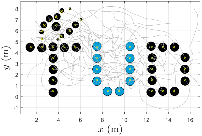
Figure 1: Rule-based Lloyd simulation result with $N=44$ holonomic robots and heterogeneous encumbrance. The robots are depicted with black and blue circles, the yellow crosses indicate the goal positions, while the paths followed by the robots are depicted with solid grey strokes. The robots start in a random position and progressively converge to their preassigned goals.

In contrast, distributed approaches in multi-robot motion planning and control involve individual robots computing their own control inputs using local information. While these methods may yield sub-optimal solutions, they offer advantages in terms of scalability and robustness compared to centralized approaches. Distributed methods are capable of handling a larger number of robots and are more resilient to communication failures or limitations. They allow robots to make decisions based on local perception, which can be beneficial in dynamic and uncertain environments.

After opting to explore distributed methods due to their significant advantages over centralized approaches, we can identify three primary categories for multi-robot motion planning and control [3]: reactive, predictive planning, learned-based methods.

I-A1 Reactive methods

are myopic by definition, hence each action is taken on the basis of the current local state. Despite being computationally efficient and usually easy to implement, deadlock conditions (local minima) as well as live-lock may occur, preventing the robots to reach the goal positions. The most popular approaches rely on velocity obstacles [4, 5, 6, 7, 8, 9, 10], force fields [11, 12, 13], barrier certificates [14, 15] and dynamic window [16].

I-A2 Predictive planning methods

use information about the neighboring robots in order to plan optimal solutions. Even though they can substantially increase the performance metrics and may avoid deadlocks by increasing the prediction horizon, usually they can be computationally expensive and/or the robots need to exchange a large amount of information through the communication network, which may not be highly reliable. Moreover, these methods may fall in live-lock conditions, which prevent the robots to converge to the goal positions. Solutions based on assigning priorities (sequential solutions) or synchronous re-planning are adopted to avoid this problem, but in the former case it introduces a hierarchy among the agents, in the latter is required a global clock synchronization. The most popular approaches rely on model predictive control (MPC) [17, 18, 19, 20, 21, 22, 23] elastic bands [24], buffered Voronoi cells [25, 26, 27], legible motion [28, 29], linear spatial separations [30]. Other interesting and recent solutions are provided by [31, 32, 33, 34, 35, 36, 37], all of them have to rely on a communication network.

I-A3 Learning-based methods

are promising and many researchers are investigating their potential [38, 39, 40, 41, 42, 43, 44, 45, 46, 47, 48, 49, 50, 51]. However, the weakness of these approaches is related to the lack of guarantees, especially for safety and convergence. In addition, the solution that these approaches provide are often non-explainable and generalization to situations different from the training scenario are hard to provide (e.g., number of robots, robots’ encumbrance, robots’ dynamics and velocities).

With respect to the state of the art algorithms, our solution allows the robots to avoid collisions and converge to their goal regions without relying on communication, without relying on the neighbors’ control inputs and without the need of synchronization. In the literature, the main approaches that rely only on neighbors positions and encumbrances, and hence do not require communication between the robots, are BVC [25], RLSS [30] and SBC [14], but none of them achieve a success rate of $1.00$ in very crowded scenarios. In fact, we tested BVC and SBC in environments with a crowdness factor $\eta=0.452$; both of them result in a success rate SR = 0.00. On the other hand, RLSS has an higher success rate, however it can experience deadlock/live-lock issues, as well as safety issues in an asynchronous setting (see [35]). This is a severe problem also due to their required computational time, which in average is $>100$ (ms).

Hence, our algorithm prove to be a valid solution in scenarios where communication between robots is unfeasible. This situation can arise from several reasons, such as security concerns, cost reduction initiatives, the necessity for interactions between diverse robots from different companies, adversarial environmental conditions, or simply for technological limitations [52]. A safe and networkless motion planning and control algorithm can find plenty of applications including but not limited to agriculture-related applications, environmental monitoring, delivery services, warehouse and logistics, space exploration, search and rescue among others.

I-B Paper Contribution and Organization

This paper proposes a distributed algorithm for multi-robot motion planning and control. Our contribution is twofold.

Firstly, we synthesize what we called the rule-based Lloyd algorithm (RBL), a solution that can guarantee safety and convergence towards the goal region. With respect to our previous work [53], here we focused on the interaction between robots and: 1) We drastically improve the multi-robot coordination performance, that is, we increased the success rate from 0.00 to 1.00 in scenarios with more that $20$ robots; 2) We provide, not only safety, but also convergence guarantees; and 3) We extend the algorithm to account for non-holonomic constraints and control inputs saturation by leveraging on a model predictive controller (MPC). Secondly, we show how the basic Lloyd-based algorithm (without rules) can be used effectively as a safety layer in learning-based methods. We present the Learning Lloyd-based algorithm (LLB), where we used reinforcement learning [54] to synthesize a motion policy that is intrinsically safe both during learning and during testing. We show that it benefits the learning phase, enhancing performance, since safety issues are already solved. By using the Lloyd-based support, in comparison to the same learning approach without the support, we measure an increase of the success rate from 0.56 to 1.00 in simple scenarios with $5$ robots, until an increase from 0.00 to 1.00 in more challenging scenarios with $50$ robots. Notice that, while RBL has guarantees with respect to the convergence to the goal, on the other hand, LLB does not ensure convergence. Nevertheless, it may perform better in terms of travel time in certain scenarios.

The paper is organized as follows. Sec. II provides the problem description. Sec. III describes the proposed algorithms. Sec. IV provides simulation results and an updated comparison with the state of the art. Sec. V provides experimental results. Finally, Sec. VI concludes the paper.

II Problem description

Our goal is to solve the following problem:

Problem 1.

Given $N$ robots, we want to steer each of them from the initial position $p_{i}(0)$ towards a goal region defined as the ball set $\mathcal{B}(e_{i},\varepsilon)$ centered in $e_{i}$, with radius $\varepsilon$. We want to do it reliably in a safe and communication-less fashion.

Assumption 1.

Each robot knows its position, its encumbrance, as well as the positions and encumbrances of its neighboring robots i.e., $j\in\mathcal{N}_{i}$ if $\|p_{i}-p_{j}\|\leq 2r_{s,i}$, where $\mathcal{N}_{i}$ denotes the set comprising the neighbors of the $i$-th robot, while $r_{s,i}=r_{s}$ is assumed to be the same for all the robots and it is defined as half of the sensing radius. In practice, both localization and neighbor detection, can be done by means of a localization module (e.g., GPS, encorders, cameras, IMU) and a vision module (e.g., cameras, Lidar) .

Assumption 2.

To provide convergence guarantees, we assume that the mission space is an unbounded convex space.

Figure 1 shows an example of a solution to the problem just described.

III Approach

The proposed approach is based on the Lloyd algorithm [55]. The main idea is to consider the following cost function

$$J_{\operatorname{cov}}({p})=\sum_{i=1}^{n}\int_{\mathcal{V}_{i}}\left\|q-p_{i}\right\|^{2}\varphi_{i}(q)dq,$$ (1)

which was originally used in [56] for static coverage control, where the positions of the robots are represented by $p=[p_{1},\dots,p_{N}]^{\top}$, $p_{i}=[x_{i},y_{i}]^{\top}$, the mission space is denoted by $\mathcal{Q}$, the weighting function that measures the importance of the points $q\in\mathcal{Q}$ is denoted by $\varphi_{i}(q):\mathcal{Q}\rightarrow\mathbb{R}_{+}$ and $\mathcal{V}_{i}$ indicates the Voronoi cell for the $i$-th robot, which is defined as

$$\mathcal{V}_{i}(p)=\left\{q\in\mathcal{Q}\mid\left\|q-p_{i}\right\|\leq\left\|q-p_{j}\right\|,\forall j\neq i\right\}.$$ (2)

Under the assumption of single integrator dynamics $\dot{p}_{i}=u_{i}$, and by following the gradient descent $\nabla J_{\text{cov}}=\frac{\partial J_{\operatorname{cov}}(p)}{\partial p_{i}}$, it follows the proportional control law

$$\dot{p}_{i}\left(\mathcal{V}_{i}\right)=-k_{p.i}\left(p_{i}-c_{\mathcal{V}_{i}}\right),$$ (3)

where the tuning parameter $k_{p,i}>0$ is a positive value, and

$$c_{\mathcal{V}_{i}}=\frac{\int_{\mathcal{V}_{i}}q\varphi_{i}(q)dq}{\int_{\mathcal{V}_{i}}\varphi_{i}(q)dq}$$ (4)

is defined as the centroid position computed over the $i$-th Voronoi cell. It can be proved that by imposing (3), by assuming a time-invariant $\varphi_{i}(q)$, each robot converges asymptotically to its Voronoi centroid position.

Our claim is that, by modifying the geometry of the cell $\mathcal{V}_{i}$ and by properly designing a weighting function $\varphi_{i}(q)$, we can obtain an efficient and effective algorithm for multi-robot motion planning and control. Notice that, while the cell geometry to provide safety was introduced by the basic LB algorithm [53, 57, 58, 59, 60], one of the novelty introduced in this work, besides the use of the algorithm as a safety layer for learning-based algorithm and the introduction of an MPC formulation to deal with dynamical constraint, is the addition of rules in the shaping of the weighting function $\varphi_{i}(q)$, which are crucial in order to increase the performance and provide convergence guarantees to the goal positions.

III-A Cell geometry $\mathcal{A}_{i}$

The reshape of the cell geometry is necessary and sufficient to provide safety guarantees. Hence, we define the cell $\mathcal{A}_{i}=\{\tilde{\mathcal{V}}_{i}\cap\mathcal{S}_{i}\}$, where

$$\tilde{\mathcal{V}}_{i}=\left\{\begin{array}[]{l}\left\{q\in\mathcal{Q}\mid\left\|q-p_{i}\right\|\leq\left\|q-p_{j}\right\|\right\}\text{ if }\Delta_{ij}\leq\frac{\left\|p_{i}-p_{j}\right\|}{2}\\ \left\{q\in\mathcal{Q}\mid\left\|q-p_{i}\right\|\leq\left\|q-\tilde{p}_{j}\right\|\right\}\text{ otherwise, }\end{array}\right.\$$ (5)

with $\Delta_{ij}=\delta_{j}+\delta_{i}$ and $\tilde{p}_{j}=p_{j}+2\left(\Delta_{ij}-\frac{\left\|p_{i}-p_{j}\right\|}{2}\right)\frac{p_{i}-p_{j}}{\left\|p_{i}-p_{j}\right\|}$, takes into account the encumbrance of the robots, while

$$\mathcal{S}_{i}=\left\{q\in\mathcal{Q}\mid\left\|q-p_{i}\right\|\leq r_{s,i}\right\}.$$ (6)

Theorem 1 (Safety).

By imposing the control $\dot{p}_{i}(\mathcal{A}_{i})$ in (3), collision avoidance is guaranteed at every instant of time.

Proof.

Since the set $\mathcal{A}_{i}=\{\tilde{\mathcal{V}}_{i}\cap\mathcal{S}_{i}\}$ is a convex set, then the centroid position $c_{\mathcal{A}_{i}}\in\mathcal{A}_{i}$. By definition of convex set, there exists a straight path from $p_{i}$ towards the centroid $c_{\mathcal{A}_{i}}$. The fact that $p_{i},c_{\mathcal{A}_{i}}\in\{\tilde{\mathcal{V}}_{i}\cap\mathcal{S}_{i}\}$ ensures that the path towards the centroid is a safe path (i.e., no other robots on the path towards the centroid), hence the control law $\dot{p}_{i}(\mathcal{A}_{i})$ as (3) always preserve safety. ∎

III-B The weighting function $\varphi_{i}(q)$

While the safety can be guaranteed by properly shaping the cell geometry, the convergence and the performance mainly depend on the definition of the function $\varphi_{i}(q)$. We adopt a Laplacian distribution centered at $\bar{p}_{i}$, which represents a point in the mission space that ultimately needs to converge to the goal location. Then we define the function $\varphi_{i}(q)$ as follows:

$$\varphi_{i}(q)=\text{exp}{\left(-\frac{\|q-\bar{p}_{i}\|}{\beta_{i}}\right)}$$ (7)

where

$$\dot{\beta}_{i}(\mathcal{A}_{i})=\begin{cases}-\beta_{i}\,\,\,&\text{if}\,\,\|c_{\mathcal{A}_{i}}-p_{i}\|<d_{1}\,\land\\ &\|c_{\mathcal{A}_{i}}-c_{\mathcal{S}_{i}}\|>d_{2}\\ -(\beta_{i}-\beta^{D}_{i})&\text{otherwise.}\end{cases}$$ (8)

and

$$\begin{split}\dot{\bar{p}}_{i}&=\begin{cases}-(\bar{p}_{i}-R(\pi/2-\epsilon)e_{i})\,\,\,&\text{if}\,\,\|c_{\mathcal{A}_{i}}-p_{i}\|<d_{3}\,\land\\ &\|c_{\mathcal{A}_{i}}-c_{\mathcal{S}_{i}}\|>d_{4}\\ -(\bar{p}_{i}-e_{i})&\text{otherwise,}\end{cases}\\ \bar{p}_{i}&=e_{i}\,\,\,\text{if}\,\,\,\|p_{i}-\bar{c}_{\mathcal{A}_{i}}\|>\|p_{i}-c_{\mathcal{A}_{i}}\|\,\land\,\bar{p}_{i}=R(\pi/2-\epsilon)e_{i}.\\ \end{split}$$ (9)

Notice that $\beta_{i}^{D},d_{1},d_{2},d_{3},d_{4}$ are positive scalar values, $R(\theta)$ indicates the rotation matrix, $\epsilon$ is a small number, $e_{i}$ is the $i$-th robot final goal position, while $\bar{{c}}_{\mathcal{A}_{i}}$ is the centroid position computed over the cell $\mathcal{A}_{i}$ with $\bar{p}_{i}\equiv e_{i}$.

Proposition 1 (Convergence).

Let us assume to have an unbounded convex space and that the initial and goal positions are adequately apart from each other i.e., $\|p_{i}(0)-p_{j}(0)\|>\Delta_{ij}$, $\|e_{i}-e_{j}\|>\Delta_{ij}$, $\forall i,j=1\dots N$ with $i\neq j$.

By imposing the control law $\dot{p}_{i}(\mathcal{A}_{i})$ in (3) and (7), (8), (9) to compute the centroid position in (4), by properly selecting $d_{1},d_{2},d_{3},d_{4}$ and $\beta^{D}_{i}$, we have that $\lim_{t\rightarrow\infty}\|p_{i}(t)-e_{i}\|<r_{s,i},\forall i=1,\dots,N.$

Proof.

The proof is structured as follows: first we ensure deadlock avoidance, then we guarantee live-lock avoidance and finally convergence.

The deadlock condition is verified when $p_{i}\equiv c_{\mathcal{A}_{i}}\equiv\bar{c}_{\mathcal{A}_{i}}\neq e_{i}$. By accounting for the effects of (8), if a robot is in a deadlock condition it means that $\beta_{i}\rightarrow 0$ and at the same time the centroid position $c_{\mathcal{A}_{i}}$ does not move, thus deadlock can occur in two situations: $i.$ if $p_{i}\equiv\bar{c}_{\mathcal{A}_{i}}\equiv{c}_{\mathcal{A}_{i}}\equiv\mathcal{A}_{i}$ and $ii.$ if $p_{i}\equiv\bar{c}_{\mathcal{A}_{i}}\equiv{c}_{\mathcal{A}_{i}}\in\partial\mathcal{A}_{i}$. Notice that $i.\implies ii.$ but not the contrary. The case $i.$ is a transitory condition if the external robots are not in condition $ii.$, hence we can only focus on the second condition. Notice that the existence of external robots is ensured by the fact that we assumed an infinite convex space.

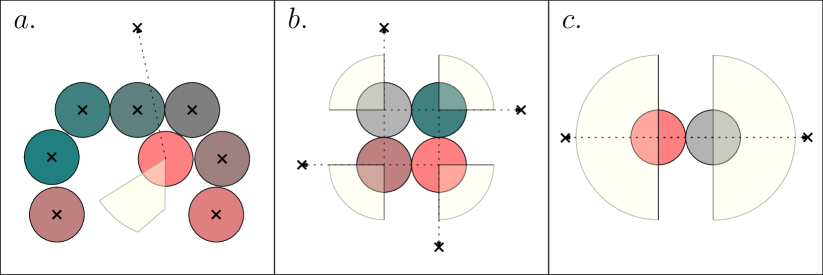
Figure 2: Theoretical deadlocking configurations, where $\beta_{i}=0$, $\forall i=1\dots N$. The crosses indicates the final goal positions for the robots (blue circles). The set $\mathcal{A}_{i}$ is depicted in yellow.

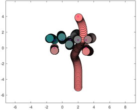
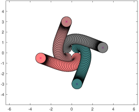
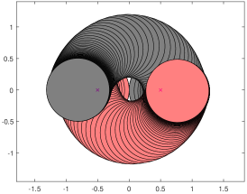
(a)	(b)	(c)

Figure 3: Simulation results starting from the theoretical deadlock conditions. The desired spreading factor is selected as $\beta^{D}=0.5$ for every robot.

For the condition $ii.$ there exist three scenarios that satisfy the deadlocking condition, we depict them in Fig. 2 for the sake of clarity, while in Fig. 3 we report the simulation results obtained by starting from the theoretical deadlock conditions. In accordance with the simulation results, we claim that the deadlocks in cases a., b., and c. cannot occur by applying the rules (8) and (9). Notice that, the introduction of these rules is the main reason why RBL over perform LB [53] in success rate. Let us analyze the three scenarios:

Case a (Fig. 2-a)

A certain number of robots have already reached their goal positions and they hinder the advancement of other robots that did not yet reached their goal locations. In this case, the value of $d_{2}$ in (8) has to be selected in such a way that $\beta_{i}$ starts to decrease after an abundant deflection from the goal, e.g., $r_{s,i}>d_{2}\geq 3\delta_{\max}$, notice that, by geometry, if $d_{2}\geq 3\delta_{\max}$ it allows the passage of the robots in any scenario. In this way, by having that $\beta_{i}^{D}>0$, each robot can be deflected from its goal position by a distance greater than $d_{2}$.

This fact can be shown by computing the distance from the centroid position analytically:

$$\left\|p_{i}-c_{\mathcal{A}_{i}}\right\|=\left\|\frac{\int_{0}^{r_{s,i}}q\,\text{exp}\left({-\frac{\left|q\right|}{\beta_{i}}}\right)dq}{\int_{0}^{r_{s,i}}\text{exp}\left({-\frac{\left|q\right|}{\beta_{i}}}\right)dq}\right\|.$$

We considered the case where we have the $i$–th robot in its goal position $e_{i}$, and a neighbor robot $j$ at distance $\Delta_{ij}=\delta_{i}+\delta_{j}$. By solving the integral we obtain

$$\left\|p_{i}-c_{\mathcal{A}_{i}}\right\|=\left\|\frac{(r_{s,i}+\beta_{i})\,\text{exp}\left({-\frac{r_{s,i}}{\beta_{i}}}\right)-\beta_{i}}{\text{exp}\left({-\frac{r_{s,i}}{\beta_{i}}}\right)-1}\right\|$$

hence, as the value of $\beta_{i}$ increases, the distance $\|p_{i}-c_{\mathcal{A}_{i}}\|$ increases as well, moreover even when the robot moves from its goal, if the value of $\beta_{i}$ does not change and the robot $j$ continues to push towards robot $i$, then the distance $\|p_{i}-c_{\mathcal{A}_{i}}\|$ does not change:

$$\begin{split}\left\|p_{i}-c_{\mathcal{A}_{i}}\right\|&=\left\|\frac{\int_{-r_{s,i}}^{0}q\,\text{exp}\left({-\frac{\left|q-Kr_{s,i}\right|}{\beta_{i}}}\right)dq}{\int_{-r_{s,i}}^{0}\text{exp}\left({-\frac{\left|q-Kr_{s,i}\right|}{\beta_{i}}}\right)dq}\right\|\\ &=\left\|\frac{-\beta_{i}\,\text{exp}\left({\frac{r_{s,i}}{\beta_{i}}}\right)+r_{s,i}+\beta_{i}}{\text{exp}\left({\frac{r_{s,i}}{\beta_{i}}}\right)-1}\right\|.\end{split}$$ (10)

In fact, $K>0$ is an arbitrary value that quantifies the distance of $e_{i}$ and it does not affect the centroid position according to (10), hence the $i$–th robot can be pushed away from its goal position by the robot $j$ at least of a quantity equal to $d_{2}$.

Case b (Fig. 2-b)

It is an unstable and unreachable equilibrium, since a small perturbation will lead to leave this configuration and moreover, it is an equilibrium only if $\beta_{i}=0$ for each robot, i.e., the centroids have to be positioned on the vertex of the cells; this is not possible since $\beta^{D}_{i}>0$ and $\beta_{i}$ evolves as (8).

Case c (Fig. 2-c)

Due to the perfect symmetry, this case would be a deadlock condition if (9) does not activate (the parameters $d_{3},d_{4}$ have to be chosen properly). Because of the directional asymmetry introduced by the right hand side behavior the robots do not fall in deadlock. The same consideration can be done in similar conditions with $N>2$.

Notice that the values $d_{1},d_{2},d_{3},d_{4}$ should depend on $r_{s,i}$, $\beta^{D}$ and ${\delta_{\max}}$ i.e., it is necessary that the conditions $\|c_{\mathcal{A}_{i}}-c_{\mathcal{S}_{i}}\|>d_{2}$ and $\|c_{\mathcal{A}_{i}}-c_{\mathcal{S}_{i}}\|>d_{4}$ can be verified , and the conditions $\|c_{\mathcal{A}_{i}}-p_{i}\|<d_{1}$ and $\|c_{\mathcal{A}_{i}}-p_{i}\|<d_{3}$ do not have to be always verified.

Once we verified deadlock avoidance, we have to check for live-lock avoidance. A live-lock condition is verified if one or more robots enter in a cyclic motion. A cyclic motion can be induce either by (8) or by (9). Notice that, if the functions $\varphi_{i}(q)$ are time-invariant, cyclic motions are not possible, since the robots converge to their centroids positions [56]. In fact, by considering $J_{\text{cov}}(p,\mathcal{A})$ (1) as a Lyapunov function:

$$\frac{d}{dt}J_{\operatorname{cov}}(p,\mathcal{A}) =\sum_{i=1}^{n}\frac{\partial}{\partial p_{i}}J_{\operatorname{cov}}(p,\mathcal{A})\dot{p}_{i}$$

$$=\sum_{i=1}^{n}2m_{i}\left(p_{i}-c_{\mathcal{A}_{i}}\right)^{T}\left(-k_{p,i}\left(p_{i}-c_{\mathcal{A}_{i}}\right)\right)$$

$$=-2k_{p,i}\sum_{i=1}^{n}m_{i}\left\|p_{i}-c_{\mathcal{A}_{i}}\right\|^{2},$$

where $m_{i}=\int_{\mathcal{A}_{i}}\varphi_{i}(q)dq$, we have convergence towards the centroid by the LaSalle’s invariance principle.

A back and forth motion can be introduced by (8), however, by construction it can happen only in the proximity of the goal and if the goal positions of two or more robots are close one each others. In fact, by properly selecting $d_{1},d_{2},\beta^{D}$, on the basis of $r_{s,i}$, then we can achieve $\|c_{\mathcal{A}_{i}}-p_{i}\|<d_{1}\implies\|c_{\mathcal{A}_{i}}-c_{\mathcal{S}_{i}}\|>d_{2}$ when $\|p_{i}-e_{i}\|>r_{s,i}$. In the case where $\|p_{i}-e_{i}\|<r_{s,i}$ this is no more necessary true, hence a back and forth motion may occur. Nevertheless, the condition $\lim_{t\rightarrow\infty}\|p_{i}(t)-e_{i}\|<r_{s,i}$ will be satisfied (see Fig. 5 with $N=300$ and associated video). To compute the values $d_{1},d_{2}$ and $\beta^{D}$ on the basis of $r_{s,i}$, we can compute the following distance

$$\begin{split}\|p_{i}-c_{\mathcal{S}_{i}}\|&=\left\|\frac{\int_{-r_{s,i}}^{r_{s,i}}q\,\text{exp}\left({-\frac{\left|q-Kr_{s,i}\right|}{\beta_{i}}}\right)dq}{\int_{-r_{s,i}}^{r_{s,i}}\text{exp}\left({-\frac{\left|q-Kr_{s,i}\right|}{\beta_{i}}}\right)dq}\right\|.\\ \end{split}$$ (11)

By considering $K\geq 1$ (i.e., $\|p_{i}-e_{i}\|>r_{s,i}$), $\beta_{i}=\beta^{D}_{i}$ and $r_{s,i}>0$, we obtain

$$\|p_{i}-c_{\mathcal{S}_{i}}\|=\left\|\frac{(r_{s,i}-\beta^{D}_{i})\,\text{exp}\left({\frac{2r_{s,i}}{\beta^{D}_{i}}}\right)+r_{s,i}+\beta^{D}_{i}}{\text{exp}\left({\frac{2r_{s,i}}{\beta^{D}_{i}}}\right)-1}\right\|$$ (12)

hence by selecting $d_{1}+d_{2}<\|p_{i}-c_{\mathcal{S}_{i}}\|$ as in (12) and $d_{1}<d_{2}$, then $\|c_{\mathcal{A}_{i}}-p_{i}\|<d_{1}\implies\|c_{\mathcal{A}_{i}}-c_{\mathcal{S}_{i}}\|>d_{2}$.

On the other hand, a periodic motion can be introduced by (9) as well. In this case, since we do not have deadlock conditions, by construction it may occur only if two or more robot have a close goal position, that is, $\|e_{i}-e_{j}\|<\Delta_{ij}$, which violate our assumption. In fact the other possible case would be when the robot is constantly hindered by other robots to reach its goal position. However, this is not possible since deadlock does not occur and because each robot can be deflected from its goal (see case a). Notice that the role of the reset condition $\bar{p}_{i}=e_{i}$ in (9) plays a crucial role since slow dynamics may lead to periodic motions.

Since all the robots converge asymptotically to their own centroid $c_{\mathcal{A}_{i}}$ by the LaSalle’s principle, and deadlock/live-lock (if $\|p_{i}-e_{i}\|>r_{s,i}$) do not occur, then all the robots will converge to their centroids’ positions (or, if live-lock occurs, inside $\mathcal{B}(e_{i},r_{s,i})$), which satisfy $\|c_{\mathcal{A}_{i}}-e_{i}\|<r_{s,i}$, hence the proof is complete.

∎

Remark 1 (Parameter Selection).

Notice that to obtain convergence, a possible selection of the parameters in (8), (9) is the following. Since the condition below must hold

$$\left\|\frac{(r_{s,i}-\beta^{D}_{i})\,\text{exp}\left({\frac{2r_{s,i}}{\beta^{D}_{i}}}\right)+r_{s,i}+\beta^{D}_{i}}{\text{exp}\left({\frac{2r_{s,i}}{\beta^{D}_{i}}}\right)-1}\right\|>3\delta_{\max},$$

then $d_{2}=d_{4}=3\delta_{\max}$, while

$$0<d_{1}=d_{3}<\left\|\frac{(r_{s,i}-\beta^{D}_{i})\,\text{exp}\left({\frac{2r_{s,i}}{\beta^{D}_{i}}}\right)+r_{s,i}+\beta^{D}_{i}}{\text{exp}\left({\frac{2r_{s,i}}{\beta^{D}_{i}}}\right)-1}\right\|-3\delta_{\max}.$$

Remark 2 (Forward Velocity).

The value of $\beta_{i}$ and $r_{s,i}$ clearly play a role on the modulus of the velocity of the $i$-th robot. By assuming to not having interactions with other robots i.e., $\mathcal{A}_{i}\equiv\mathcal{S}_{i}$, we can analytically compute the distance of the $i$-th robot from the centroid $c_{\mathcal{A}_{i}}$ and hence the velocity, in fact by definition we have

$$\begin{split}\|p_{i}-c_{\mathcal{A}_{i}}\|&=\left\|\frac{\int_{-r_{s,i}}^{r_{s,i}}q\,\text{exp}\left({-\frac{\left|q-Kr_{s,i}\right|}{\beta_{i}}}\right)dq}{\int_{-r_{s,i}}^{r_{s,i}}\text{exp}\left({-\frac{\left|q-Kr_{s,i}\right|}{\beta_{i}}}\right)dq}\right\|.\\ \end{split}$$ (13)

If $K\geq 1$ and $r_{s,i}>0$, we obtain

$$\|p_{i}-c_{\mathcal{A}_{i}}\|=\left\|\frac{(r_{s,i}-\beta_{i})\,\text{exp}\left({\frac{2r_{s,i}}{\beta_{i}}}\right)+r_{s,i}+\beta_{i}}{\text{exp}\left({\frac{2r_{s,i}}{\beta_{i}}}\right)-1}\right\|$$ (14)

on the other hand when $0<K<1$ we have

$$\|p_{i}-c_{\mathcal{A}_{i}}\|=\left\|\frac{\rho_{i}\text{exp}\left(\frac{r_{s,i}(K-1)}{\beta_{i}}\right)-\rho_{i}\text{exp}\left(-\frac{r_{s,i}(K+1)}{\beta_{i}}\right)-2Kr_{s,i}}{\text{exp}\left(\frac{r_{s,i(K-1)}}{\beta_{i}}\right)+\text{exp}\left(-\frac{r_{s,i(K+1)}}{\beta_{i}}\right)-2}\right\|,$$ (15)

where $\rho_{i}=r_{s,i}+\beta_{i}$, by exploiting (3) and (13) we have a map between $\beta_{i}$ and the $i$-th robot’s velocity, in the case of non deformed cells, which may be regarded as standard operating conditions.

It is important to highlight that the centroid position remains unaffected by the value of $K$ if $K>1$, see (14). This implies that regardless of where the Laplacian function (7) is centered, as long as its mean value is at a distance greater than or equal to $r_{s,i}$, the centroid distance will only depend on $\beta_{i}$ and $r_{s,i}$. On the other hand if $0<K<1$, it means that $\|p_{i}-e_{i}\|=Kr_{s,i}<r_{s,i}$, hence the centroid position has to depend on $K$, accordingly to (15). In light of these results, the velocity $\|\dot{p}_{i}\|=k_{p,i}\|p_{i}-c_{\mathcal{A}_{i}}\|$, in standard operating condition for the robot $i$, can be designed through $k_{p,i}$ or $\beta_{i}^{D}$.

Remark 3 (Pushing Effect).

Another important insight is related to the pushing effect. According to Remark 2 the distance of the centroid from the robot does not depend on the mean value of the function $\varphi_{i}(q)$, if it is at a distance greater than $r_{s,i}$. This is true also if robots interact, in fact, by solving (10) it is clear that if $\beta_{i}>\beta_{j}$ then $\|p_{i}-c_{\mathcal{A}_{i}}\|>\|p_{j}-c_{\mathcal{A}_{j}}\|$, hence it results in a pushing effect, i.e., robot $j$ will push robot $i$. In this scenario is possible to compute analytically the equilibrium distance between robot $i$ and robot $j$ by solving

$$0=\frac{d}{dt}\left\|\frac{\int_{-r_{s,i}}^{p_{i}(t)-p_{j}(t)-2\Delta_{i,j}}q\,\text{exp}\left(\frac{-|q-Kr_{s,i}|}{\beta_{i}}\right)dq}{\int_{-r_{s,i}}^{p_{i}(t)-p_{j}(t)-2\Delta_{i,j}}\text{exp}\left(\frac{-|q-Kr_{s,i}|}{\beta_{i}}\right)dq}\right\|.$$

By imposing $p_{j}=0$ and solving it for $p_{i}$, we compute the equlibrium distance $d^{\star}$ between robot $i$ and $j$. Then the $i$-th robot velocity reads as follows:

$$\|\dot{p}_{i}\|=k_{p,i}\left\|\frac{\int_{-r_{s,i}}^{d^{*}-2\Delta_{i,j}}q\,\text{exp}\left(\frac{-|q-Kr_{s,i}|}{\beta_{i}}\right)dq}{\int_{-r_{s,i}}^{d^{\star}-2\Delta_{i,j}}\text{exp}\left(\frac{-|q-Kr_{s,i}|}{\beta_{i}}\right)dq}\right\|.$$

Remark 4 (Numerical Simulations and Asynchrony).

Notice that the simulations in Sec. IV are implemented in discrete time and with discretized cells $\mathcal{A}_{i}$, since computing the centroid position $c_{\mathcal{A}_{i}}$ in closed form it is not always possible. Hence, $\beta_{i,\min}$ has to be set together with the cell discretization d$x$. While $k_{p,i}$ has to be selected on the basis of the time discretization d$t$. In particular, to preserve safety, it is easy to verify from (3) that $k_{p,i}$d$t\leq 1$, while to preserve convergence and performance the cell discretization should be reasonably small. In the simulations in Sec. IV we selected d$x=0.075$ (m), d$t=0.033$ (s).

Notice that the proposed algorithm can also work in an asynchronous setting i.e., each robot can take an action at a different time. In fact, in order to not have safety issues in an asynchronous setting, it would be sufficient to have $k_{p,i}$d$t\leq\frac{\|p_{i}-c_{\mathcal{A}_{i}}\|-\delta_{i}}{\|p_{i}-c_{\mathcal{A}_{i}}\|}$ and since $\|p_{i}-c_{\mathcal{A}_{i}}\|<r_{s,i}$, we can conclude that $k_{p,i}$d$t\leq 1-\frac{\delta_{i}}{r_{s,i}}$. By considering d$t$ equal to the computational time, this is not a strict assumption according to the computational time required by the algorithm (see Sec. IV-H).

III-C Learning policy with Lloyd-based support (LLB)

The choices behind the selection of $\beta_{i}$ (8) and $\bar{p}_{i}$ (9) are crucial to obtain acceptable performance and convergence. In the previous section we introduced a way to achieve convergence with acceptable performance. However, the selection of $\beta_{i}$ (8) and $\bar{p}_{i}$ (9) is far from optimal i.e., a lower travel time can be achieved. Hence we propose to select these values by means of a learned function. By relying on learning-based techniques the convergence cannot be guaranteed anymore, but the safety is still ensured, both during training and testing, as it does not depend on $\beta_{i}$ and $\bar{p}_{i}$. While prior works on learned navigation tasks require to properly shape the reward function to avoid collisions and at the same time to converge to the goal, our method allows to focus on learning how to reach the goal as quickly as possible.

Similarly to [54], we learn a high-level attention-based navigation policy that encodes the goal relative position and the relative positions and velocities of the other robots in the neighborhood (notice that the velocity is computed by relying on the past and actual positions). The learned latent representation is mapped to the parameters of a diagonal Gaussian distribution that we sample to obtain $\beta_{i}$ and $\bar{p}_{i}$.

III-C1 RL Formulation

Similarly to [47], the observation vector of each robot $i$ is composed of its own information and relative states of all robots $j$ within its sensing range:

$${s}^{t}_{i}=[\Delta p_{e,i},\dot{p}_{i},\delta_{i},l_{i}]$$ (16)

$${s}^{t}_{j}=[\Delta p_{j,i},\dot{p}_{j},\delta_{j}],\quad\forall j\in\mathcal{N}_{i},$$

where ${s}^{t}_{i}$ and ${s}^{t}_{j}$ are the available information that robot $i$ has of itself and other robots $j$ in its sensing range. Notice that these information are obtained by relying on the onboard sensors. The relative positions of the goal and other robots are represented by $\Delta p_{e,i}$ and $\Delta p_{j,i}$ While the hyper-parameter $l_{i}$ is initialized as $l_{i}=0$, it becomes equal to $1$ when $p_{i}\in\mathcal{B}(e_{i},\varepsilon)$ and it stays equal to $1$ until $p_{i}\notin\mathcal{B}(e_{i},\varepsilon+d)$, where $d>0$ is an arbitrary distance. All positions and velocities are represented in polar coordinates. We denote the joint observed state of all robots in $\mathcal{N}_{i}$ by $\mathcal{O}^{t}_{i}$.

We seek to learn the optimal policy for each robot $i$: $\pi_{i}(s^{t}_{i},\mathcal{O}^{t}_{i})$, that maps its observation of the environment to an action vector: ${a}^{t}_{i}=(\Delta\bar{p}_{i},\beta_{i})$ with $\Delta\bar{p}_{i}=\bar{p}_{i}-p_{i}$, eventually guiding the robot towards its goal. Since placing $\bar{p}_{i}$ beyond $r_{s,i}$ does not have any effect on $c_{\mathcal{A}_{i}}$ (see Remark 2), the action space is bounded by $\Delta\bar{p}_{i}\in\mathcal{B}(0,r_{s,i})$, while we contrained $\beta_{i}\in[0.1,0.5]$.

We design the reward function to motivate the ego-robot to reach and maintain its goal position while allowing other robots to reach theirs. The reward attributed to each robot $W_{i}$ is defined as:

$$W_{i}({s}_{i}^{t+1},\mathcal{O}_{i}^{t+1},{a}_{i}^{t},{s}_{i}^{t},\mathcal{O}_{i}^{t})=W_{t,i}+W_{g,i},$$ (17)

where $W_{t,i}=w_{t}-\Delta p_{e,i}$, and

$$\ W_{g,i}=\begin{cases}w_{g}&\quad\text{if }l_{i}^{t+1}-l_{i}^{t}=1\\ 0&\quad\text{if }l_{i}^{t+1}-l_{i}^{t}=0\\ -w_{g}&\quad\text{if }l_{i}^{t+1}-l_{i}^{t}=-1\end{cases}$$

with $\Delta p_{e,i}$ being the distance from robot $i$ to its goal, and $w_{g}$ and $w_{t}$ being the reward for robot $i$ achieving its goal, and the punishment for each time step that all robots have not achieved their goal, respectively. Note that there is no need for punishing collisions. Since the low-level controller always tracks the centroid of the cell, which now depends on the learned parameters $\bar{p}_{i}=p_{i}+\Delta\bar{p}_{i}$ and $\beta_{i}$, collisions cannot happen by definition. The episode ends when all the robots are within a distance $\epsilon$ of their goals or the time step limit has been reached.

III-C2 Policy Network Architecture

Similar to [54] we learn a high-level attention-based policy that outputs the action vector ${a}^{\prime}_{i}=(\Delta\bar{p}^{\prime}_{i},\beta^{\prime}_{i})$ conditioned to its observation of the environment. The architecture of the learned policy, shown in Figure 4 follows the encoder-decoder network paradigm [54, 61]. The available information of the environment (e.g. the goal and a variable number of agents inside the sensing range) is encoded through a self-attention network (SAB) that learns how each element’s representation should be affected by the presence of others. Then a multi-headed attention layer is used to pool the resulting latent representations conditioned to $s^{t}_{i}$. The resulting vector is then mapped through a fully connected layer to the parameters of a diagonal Gaussian distribution and an estimate of the state-value. The diagonal Gaussian distribution is then sampled to obtain ${a}^{\prime}_{i}=(\Delta\bar{p}^{\prime}_{i},\beta^{\prime}_{i})$, which is remapped to the action-space bounds. The state-value estimate is used only during training by the algorithm used to train the architecture.

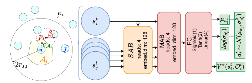
Figure 4: Overview of the learned policy network. The observed robots are encoded through a self-attention layer (SAB) and decoded with a multi-headed attention layer that takes $s_{i}$ as query. The resulting vector is mapped to the parameters of the diagonal Gaussian distribution, $\mathcal{N}(\mu_{a^{\prime}_{t}},\sigma^{2}_{a^{\prime}_{t}})$, and value function estimate, $V^{\pi}(s^{t}_{i},\mathcal{O}^{t}_{i})$.

We employ the Proximal Policy Optimization (PPO) for training our neural network [62] with parameter-sharing. In our implementation [63], we utilize a combination of the surrogate loss and the KL-divergence term to ensure training stability. Additionally, an entropy regularization term is integrated to foster exploration, as outlined in [64]. For a deeper dive into the algorithm’s details, we direct readers to [62].

III-C3 Further considerations

To guide and stabilize learned policy, we introduce a number of modifications both during training and testing. Firstly, to smooth our trajectories, we estimate $a_{i}^{t}$ by running an unbiased exponential recency-weighted average [65]:

$$a_{i}^{t+1}=\frac{\alpha}{o^{t}}a^{\prime}_{i}+(1-\frac{\alpha}{o^{t}})a^{t}_{i}$$ (18)

$$o^{t+1}=o^{t}+\alpha(1-o^{t})\text{, with $o^{0}=0$,}$$

where $\alpha$ is a hyperparameter that modulates how reactive is the policy to the output of the learned network. Secondly, we also assume that pushing (see Remark 3) is only necessary when the robot has not completed its tasks. Therefore, the output $\beta^{\prime}_{i}$ is clipped to the lower values $[0.1,0.28]$ if $l_{i}=1$, and it is clipped to the higher values $[0.32,0.5]$ otherwise. This allows the robot to be more aggressive when the goal has not been achieved, and let other robots pass while it is near its goal. We also substitute $\bar{p}^{\prime}_{i}$ by the goal position $e_{i}$ when $l_{i}=1$ to ensure stationary behavior when robots are at their goal, making the pushing effect easier to learn. We refer to the overall method as Learning Lloyd-based method (LLB). In the simulation results in Sec. IV, we show the advantages of LLB with respect to the pure learning method without the Lloyd-based support.

III-D Dynamic constraints

Until now we only discussed the case of holonomic robots, however it is possible to implement the proposed algorithm also on unicycle and car-like robots. In fact, as we discussed, the holonomic robot has just to pursue a point position (i.e., the centroid $c_{\mathcal{A}_{i}}$). Similarly to [66], we use an MPC formulation to generate control inputs for the robots, which are compliant with the robot dynamics and that at each iteration would generate a trajectory that always remains inside the cell $\mathcal{A}_{i}$. In this way we can still guarantee safety at every time step. Each robot $i$ solves the following MPC problem (we omit the $i$ indexing to simplify the notation),

$$\min_{{x}_{k},{u}_{k}} \sum^{N_{t}}_{k=0}J_{k}({x}_{k},{u}_{k},c_{\mathcal{A}})$$ (19a)

s.t.: $${x}_{k}=f({x}_{k-1},{u}_{k-1}),$$ (19b)

$$\,{x}_{k}\in\mathcal{X},\,{u}_{k}\in\mathcal{U},$$ (19c)

$$p_{k}\in\mathcal{A}$$ (19d)

$${x}_{0}={x}_{\textrm{init}},$$ (19e)

where $k$ indicates the time index, $N_{t}$ is the number of time instants in the MPC problem, $J$ is the cost function, ${x}_{k}$ and ${u}_{k}$ are the state and inputs respectively, $f({x}_{k-1},{u}_{k-1})$ is the dynamic constraint that represents the specific robot dynamics, ${x}_{k}\in\mathcal{X},\,{u}_{k}\in\mathcal{U}$ are the state and input constraints respectively, and ${x}_{0}={x}_{\textrm{init}}$ is the initial condition. The cost $J$ for each time instant $k$ is defined as:

$$J_{k}=\left(\langle{v}_{k},(c_{\mathcal{A}}-p_{k})\rangle-v^{D}\right)^{2}+{u}_{k}^{\top}Q{u}_{k},$$ (20)

where $\langle\cdot,\cdot\rangle$ indicates the inner product, ${v}_{k}$ is the robot’s velocity in the $x$-$y$ plane, $v^{D}$ is the target absolute velocity that may be defined as a function of the distance from the centroid, i.e. $v^{D}=v^{D}(\|c_{\mathcal{A}}-p_{k}\|)$ and $Q$ is a positive definite matrix of weights.

Note that since each robot has a certain encumbrance, the maximum number of constraints introduced by (19d) is $n_{c}^{\max}=\frac{2\pi r_{s,i}}{\delta_{j}}$. This is particularly useful when implementing the MPC in practice, since in order to achieve high computational speed at runtime, tools such as Forces-pro [67], [68], require to pre-compile the full optimization problem. It is important to note that since we have now introduced potentially complex robot dynamics (19b) as well as actuator and state constraints, we can not guarantee the recursive feasibility of the MPC problem (19). This may happen if for example, the sensing range is small and the robots have limited braking capability. It is however to be noted that in practice, for adequate sensing range and target velocity values, this is not an issue.

IV Simulation results

The proposed approach is tested in simulation in several scenarios. We also provide a comparison with state of the art approaches. Through these numerical simulations we aim to further prove the scalability, the robustness, and the flexibility of the proposed approach. The video [69] that accompanies the paper provides additional simulations to show the performance of the method. The source code can be found at https://github.com/manuelboldrer/RBL.

The parameters are selected as follows: $r_{s,i}=1.5$ (m). Because of numerical issues due to the fact that the centroid position is not computed analytically but numerically, we also set a minimum value for $\beta_{i,\min}=0.1$. Notice that the values for the parameters $d_{1}=d_{3},d_{2}=d_{4}$ have to depend on $r_{s,i}$ and $\beta_{i}^{D}$ for a correct convergence (see Proposition 1 and Remark 1).

The performance metrics that we considered include the maximum travel time (max time), which measures how much it takes to all the robots to converge towards their goal positions, the average speed of each robot during the mission (for each robot the mission stops when it reaches its goal position), and the robots success rate (RSR), computed as the ratio of robots that safely reached the goal to the total number of robots.

IV-A Crossing circle (RBL)

We report several simulations in the crossing circle scenario. In Fig. 5 we depicted the trajectories obtained by considering $N=[5,10,25,50,300]$ homogeneous holonomic robots. The radius of the circle is $R_{c}=[10,10,10,10,15]$ (m). The value of $\beta_{i}^{D}=0.5$, $\forall i=1,\dots,N$. The robot encumbrance $\delta_{i}=[0.35,0.35,0.35,0.35,0.1]$ (m), and $k_{p,i}=6$, $\forall i=1,\dots,N$.

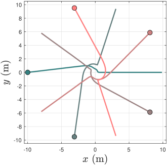
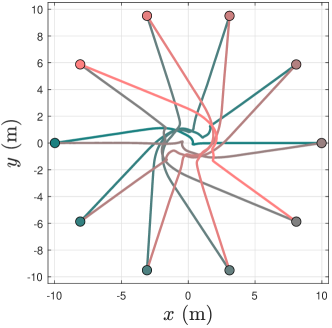
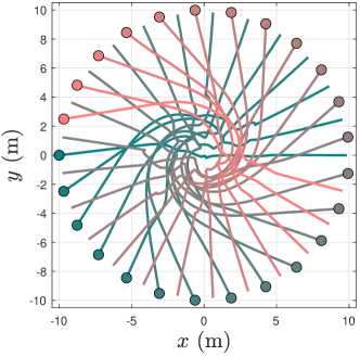
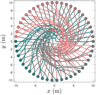
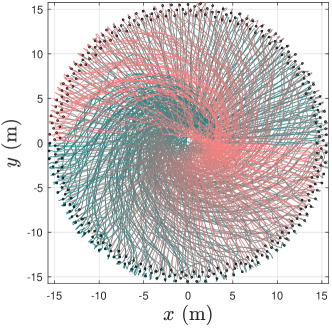
Figure 5: Circle crossing: simulation results with $N=[5,10,25,50,300]$ holonomic robots. The value $\beta^{D}=0.5$ is the same for all the robots.

N	$\eta$	max time (s)	mean speed (m/s)	succ. rate
5	0.0061	5.18	3.96	1.00
10	0.0122	5.91	3.73	1.00
25	0.0306	7.98	2.91	1.00
50	0.0612	11.09	2.40	1.00
300	0.0133	30.76	1.52	1.00

Table I: Circle crossing: quantitative data form the simulation in Figure 5.

In Table I we report the quantitative results, where $N$ is the number of robots and $\eta=\frac{\text{Area}_{\text{robots}}}{\text{Area}_{\text{tot}}}$ is what we called the crowdness factor, which is the ratio between the sum of the area occupied by the robotsand the total mission space area, it is an indicator of the challenging and intricate nature of the considered scenario.

In Figure 6 we show other two simulations, where we picked a random encumbrance radius for each robot $\delta_{i}\in[0.1,0.5]$. On the left hand side we selected $\beta^{D}_{i}=0.5$, $\forall i=1,\dots,N$, while on the simulation on the right hand side we selected $\beta^{D}_{i}\in[0.2,1.5]$ randomly for each robot. Figure 7 shows the effects of the choice of $\beta^{D}$ on the travel time for each robot, in accordance with Remark 2, by increasing $\beta^{D}$ the travel time increases as well.

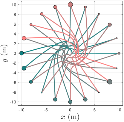
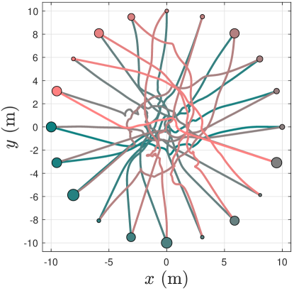
Figure 6: Circle crossing: simulation results with $N=20$ holonomic robots with random encumbrance $r$. On the left hand side $\beta^{D}_{i}=0.5$ for all the robots, On the right hand side $\beta^{D}_{i}$ is random and different from robot to robot.

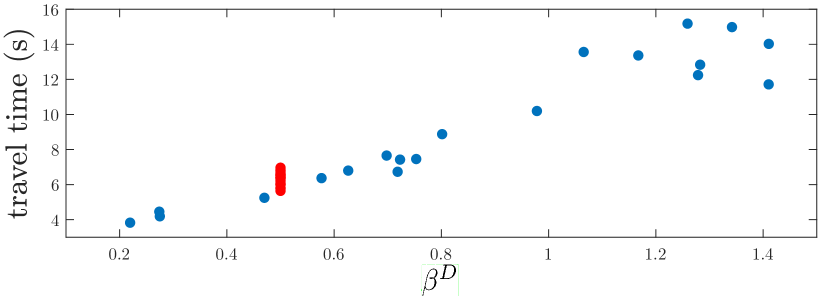
Figure 7: Dependence of the travel time with respect to $\beta^{D}_{i}$. Each dot represents the performance of one robot. In red the left hand side simulation in Figure 6, in blue the right hand side simulation in Figure 6.

IV-B Half crossing circle (RBL)

Similarly to the crossing circle case, we report some simulations for the half crossing circle scenario. In this case, the goal position for each robot is shifted by an angle of $\pi+\gamma$, rather than being exactly out of phase by $\pi$. In Figure 8, we show that even if the robots follow the right hand side rule according to (9), our algorithm can also manage this challenging situations, where the emergent behavior is a clockwise rotation. In Table II we report the quantitative results.

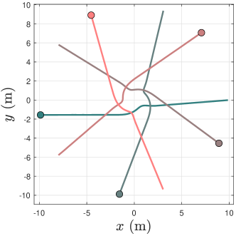
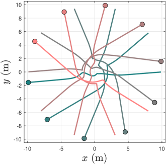
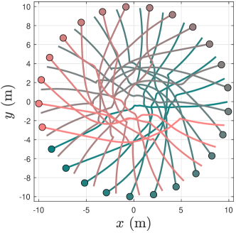
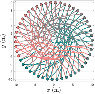
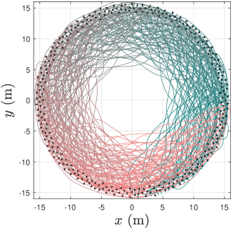
Figure 8: Half circle crossing: simulation results with $N=[5,10,25,50,300]$, holonomic robots. The value $\beta^{D}=0.5$ is the same for all the robots. The goal position is rotated with respect to the crossing scenario of a value $\gamma=[\pi/20,\pi/20,\pi/6,\pi/6,\pi/2]$.

N	$\eta$	max time (s)	mean speed (m/s)	succ. rate
5	0.0061	5.05	3.95	1.00
10	0.0122	5.44	3.77	1.00
25	0.0306	6.47	3.43	1.00
50	0.0612	7.01	2.76	1.00
300	0.0133	16.59	1.91	1.00

Table II: Half circle crossing: quantitative data form the simulation in Fig. 8.

IV-C Random room (RBL)

In this scenario we report two simulations. The initial location and the final goal location are selected randomly. In Figure 9, on the left hand side, $\eta_{1}=0.157$ and $N=20$ homogeneous robots, on the right hand side $\eta_{2}=0.135$ and $N=300$ heterogeneous (random size) robots. In both cases the robots successfully converge to a neighborhood of the goal positions.

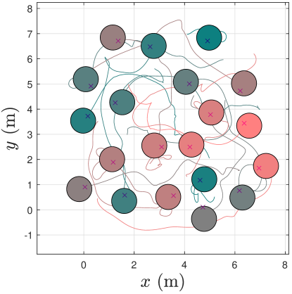
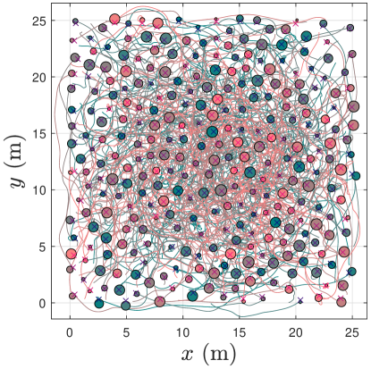
Figure 9: (left) Room 7x7 (m²): simulation results with $N=20$ holonomic robots with crowdness factor $\eta=0.157$. (right) Room 25x25 (m²): simulation results with $N=300$ holonomic robots with crowdness fator $\eta=0.135$ and random encumbrance $\delta$.

IV-D Learning approach (LLB)

We implemented the Learning Lloyd-based (LLB) algorithm introduced in Section III-C, to verify the effectiveness of using a Lloyd-based support on learning-based algorithms. In Table III we compared the same learning algorithm, with the Lloyd support (LLB), without the support of the LB algorithm (Pure Learning), and also with the RBL algorithm.

We made few changes to train the learning approach without Lloyd support. In fact in this case, we only learn a point relative to the robot $\Delta\tilde{p}_{i}\in\mathcal{B}(0,r_{s,i})$, to follow with velocity $\dot{p}_{i}=v_{i,\text{max}}\frac{\Delta\tilde{p}_{i}}{r_{s,i}}$. Since collisions under this policy are possible, additional reward signal $r_{\text{coll}}$ is also added to the reward function to punish collision events. All other conditions have been maintained. We observed that the addition of LB during training simplifies the problem. Pure learning method requires trading off collision avoidance with fast goal convergence. Instead, adding the safety LB layer during training allows to only consider fast convergence towards the goal. We run multiple simulations in different scenarios. It results that the LLB was able to achieve a success rate of $1.00$, while pure learning presents failures even in simple scenarios (e.g., with $N=5$). With respect to RBL, the LLB performs better in symmetric scenarios (i.e., circle scenarios) and worse in the random room scenarios. In Figure 10 we depict the trajectories obtained from LLB in the crossing circle scenarios reported also in Table III.

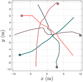
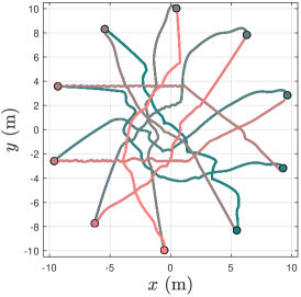
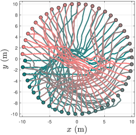
Figure 10: Crossing circle: simulation results with $N=[5,10,50]$ holonomic robots, by using LLB approach.

RBL	$N$	$\eta$	max time (s)	succ. rate
circle ($10$ m)	5	0.0045	6.56	1.00
room ($9\times 9$ m2)	5	0.0289	2.25	1.00
circle ($10$ m)	10	0.0090	7.78	1.00
room ($9\times 9$ m2)	10	0.0349	2.74	1.00
circle ($10$ m)	50	0.0450	17.65	1.00
room ($15\times 15$ m2)	50	0.0628	12.36	1.00
Pure Learning	$N$	$\eta$	max time (s)	succ. rate
circle ($10$ m)	5	0.0045	5.25	0.94
room ($9\times 9$ m2)	5	0.0289	2.79	0.56
circle ($10$ m)	10	0.0090	6.38	0.77
room ($9\times 9$ m2)	10	0.0349	3.31	0.04
circle ($10$ m)	50	0.0450	-	0.00
room ($15\times 15$ m2)	50	0.0628	-	0.00
LLB	$N$	$\eta$	max time (s)	succ. rate
circle ($10$ m)	5	0.0045	5.47	1.00
room ($9\times 9$ m2)	5	0.0289	2.42	1.00
circle ($10$ m)	10	0.0090	6.43	1.00
room ($9\times 9$ m2)	10	0.0349	3.37	1.00
circle ($10$ m)	50	0.0450	13.35	1.00
room ($15\times 15$ m2)	50	0.0628	13.67	1.00

Table III: Simulation results for rule-based Lloyd (RBL), Pure Learning and Learning with Lloyd support (LLB). We considered $N=[5,10,50]$ holonomic robots in the crossing circle scenario and in the random room scenario, with robot encumbrance $\delta_{i}=0.3$ (m). The maximum time is an average of the successful simulations.

IV-E Dynamical constraints (RBL)

We also tested our algorithm with different dynamical models, i.e., the unicycle and the car-like. In Figure 11 we depicted the results in the crossing circle scenario for $N=[5,10,25]$, for the unicycle model (top) and for the car-like model (bottom). In both cases we set a maximum and desired forward velocity $v^{D}=1.5$ (m/s). The quantitative results are reported in Tables IV and V.

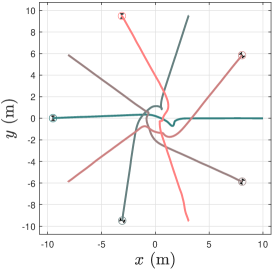
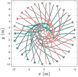
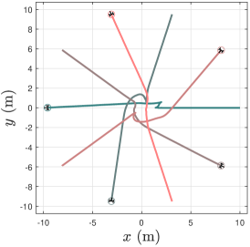
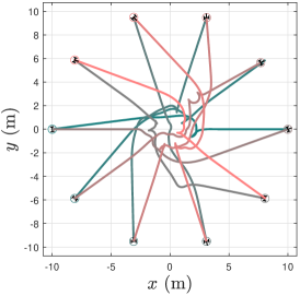
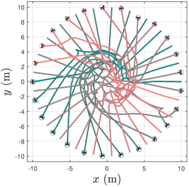
Figure 11: Crossing circle: simulation results with $N=[5,10,25]$ non-holonomic robots. On the top the unicycle model, on the bottom the car-like model.

N	$\eta$	max time (s)	mean speed (m/s)	succ. rate
5	0.006125	21.50	1.09	1.00
10	0.01225	26.60	1.01	1.00
25	0.0306	32.90	0.82	1.00

Table IV: Circle crossing unicycles: quantitative data from the simulation in Fig. 11 (top).

N	$\eta$	max time (s)	mean speed (m/s)	succ. rate
5	0.006125	26.90	0.86	1.00
10	0.01225	32.00	0.80	1.00
25	0.0306	44.40	0.64	1.00

Table V: Circle crossing car-like: quantitative data from the simulation in Fig. 11 (bottom).

IV-F Robustness and reliability (RBL)

For the crossing circle and random room in the holonomic case we run additional simulations to test the robustness of the algorithm to the change in parameters. According to the data reported in [44] Sec. $5.4$, it is clear that in learning-based solutions performance, safety and convergence degrade by changing parameters such as the dimension of the robots and the desired velocity. In the following we show an analysis of robustness by considering an heterogeneous scenario and by selecting randomly the dimension of the robots between $\delta_{i}\in[0.1,0.5]$, the value of $\beta^{D}_{i}\in[0.2,0.75]$ and $k_{p,i}\in[3,6]$. We run $100$ simulations with $N=[20,40,100]$ robots. The simulation results are reported in Table VI, the success rate is always equal to $1.00$.

RBL	$N$	mean of $\eta$	max time (s)	mean speed (m/s)	RSR
circle ($4$ m)	20	0.112	8.87$\pm$ 0.98	1.70 $\pm$ 0.10	1.00
room ($7\times 7$ m2)	20	0.115	5.33 $\pm$ 1.13	1.79 $\pm$ 0.25	1.00
circle ($7$ m)	40	0.073	12.96 $\pm$ 0.84	1.80 $\pm$ 0.11	1.00
room ($9\times 9$ m2)	40	0.139	10.24 $\pm$ 2.16	1.46 $\pm$ 0.07	1.00
circle ($16$ m)	100	0.0352	24.57 $\pm$ 1.15	2.03 $\pm$ 0.10	1.00
room ($15\times 15$ m2)	100	0.125	21.83 $\pm$ 4.89	1.46 $\pm$ 0.07	1.00

Table VI: Simulation results for $N=[20,40,100]$ robots in the crossing circle scenario and in the random room scenario, with $\delta_{i}\in[0.1,0.5]$ (m), $\beta^{D}_{i}\in[0.2,0.75]$ and $k_{p,i}\in[3,6]$.

IV-G Comparison with state of the art

As we already mentioned, our main advantages with respect to the algorithms proposed in the literature reside in the combination of four aspects:

1. We can achieve success rate of $1.00$ in very crowded scenarios. 2. Each robot needs to know only its position $p_{i}$, its encumbrance $\delta_{i}$, its goal position $e_{i}$, its neighbours’ positions $p_{j}$ and encumbrance $\delta_{j}$ (if $\|p_{i}-p_{j}\|\leq 2r_{s,i}$, then $j\in\mathcal{N}_{i}$); 3. The control inputs for each robot can be generated in an asynchronous fashion without affecting safety and convergence. 4. We can account for heterogeneous conditions, i.e., different robots’ encumbrances and different robots’ dynamics and velocities;

The combination of these features are not provided by any other algorithm in the literature. In the following, we provide a comparison with some state of the art algorithms.

Firstly, we considered the non-holonomic (unicycle) case, we compared the performance of our rule-based Lloyd algorithm (RBL) with LB [53] and RL-RVO [41], which demonstrates superior performance and success rate compared to other algorithms such as SARL [48], GA3C-CADRL [49], NH-ORCA [6].

We considered the crossing circle scenario $R_{c}=4$ (m) with $N=[6,20,30]$, $\delta_{i}=0.2$ (m), a maximum forward velocity $v_{i,\max}=1.5$ (m/s) and limits on the accelerations of $a_{i,\max}=1$ (m/s²). As a result (see Table VII), RBL executes better in terms of success rate with respect to the other algorithms (in this case the success rate is the ratio between the number of missions where the robots converged safely and the total number of missions simulated). On the other hand, when it succeed, RL-RVO has in average better performance. This is also due to the fact that RL-RVO relies on stronger assumptions (each robot has to collect exteroceptive observations).

We also propose a comparison with other reactive algorithms for the holonomic robots case, such as RVO2 [70], SBC [14] and also with recent predictive planning methods such as BVC [25], DMPC [71] and LCS [72]. Even if some of these algorithms may have better performance in terms of time to reach the goal in certain scenarios, they lack of guarantees of live-lock and deadlock avoidance, hence, even in simple scenarios they may fail the mission. In [72] (Sec. IV, Fig. 5) it is clear that the success rate of the mission decreases considerably for $N>50$, as well for BVC, DMPC and LCS. Also RVO2 [70] presents deadlock issues in symmetric conditions (crossing circle) and in crowded random room scenarios with high crowdness factor e.g., we tested a random room scenario with $\eta=0.452$, it results in a SR $=0.65$. Finally, for the SBC approach [14], in Sec. VII is clearly stated that the algorithm suffers of what they called type III deadlock and live-lock as well. We tested it in a scenario with $\eta=0.452$, it results in SR $=0.00$. In the same scenario our RBL reached SR $=1.00$.

In conclusion, with respect to the state of the art, our RBL algorithm often achieves similar performance in terms of time to reach the goal, nevertheless it consistently attains a success rate of 1.00, and it does so without relying on exteroceptive observations (e.g., future intentions of the other robots), the neighbours velocities, or synchronization between the robots. For the best of our knowledge, this is not provided by any other distributed algorithm in the literature. However, we want to underline that if a reliable communication network and a good computational power are available, then IMPC-DR [36] and ASAP [37] are valid solutions that provide a success rate of SR $=1.00$.

	$N$	$\eta$	max time (s)	mean speed (m/s)	succ. rate
	6	0.015	7.10	1.19	1.00
RL-RVO [41]	20	0.05	13.84	0.73	0.71
	30	0.075	21.89	0.62	0.10
	$N$	$\eta$	max time (s)	mean speed (m/s)	succ. rate
	6	0.015	13.42	0.66	1.00
LB [53]	20	0.05	-	-	0.00
	30	0.075	-	-	0.00
	$N$	$\eta$	max time (s)	mean speed (m/s)	succ. rate
	6	0.015	9.86	0.89	1.00
RBL (ours)	20	0.05	17.85	0.65	1.00
	30	0.075	26.16	0.59	1.00

Table VII: Circle crossing: quantitative data with unicycle model. We compared our method (RBL) with LB [53] and RL-RVO [41] method, since SARL [48], GA3C-CADRL [49] and NH-ORCA [6] underperform it according to [41]. Notice that in RL-RVO, each robot has to collect exteroceptive observations i.e., the method relies on a communication network.

IV-H Computational time

The computational time of the proposed approach depends mainly on $r_{s,i}$ (assuming a fixed space discretization step d$x=0.075$ (m)), since we compute the centroid position numerically. We tested the algorithm in Python on an AMD Ryzen 7 5800H. By considering that $r_{s,i}$ should be limited to a maximum amount of $2$ (m) (notice that $r_{s,i}$ is half the sensing radius capability) a real-time implementation is largely feasible. In fact we measured for $r_{s,i}=2.0$ (m) an average computational time of $t_{c}=10$ (ms), for $r_{s,i}=1.5$ (m) we measured $t_{c}=5.5$ (ms), while for $r_{s,i}=1.0$ (m) the computational time reduces to $t_{c}=2$ (ms). The addition of the MPC to account for dynamic constraints has an impact on the computational time. However, despite a clear increase in the computational time, it does not prevent to be used for real-time applications (as it is shown in the experimental result section V). We measured an increase of $16$ (ms) on average.

V Experimental results

We tested our RBL algorithm on $N=3$ scaled-down car-like robots with $\delta_{i}=0.15$ (m), the robots consist of a modified Waveshare JetRacer Pro AI kit. Due to the limited sensing capabilities of the robots, the real-time positions are obtained through an OptiTrack motion capture system. In the following, we report the results obtained from a crossing circle scenario and a random room scenario with $N=3$. In both the scenarios the robots converge safely to their goal positions, in accordance with the theory and the simulation results. The dynamic constraint (19b) is now described as the following kinematic bicycle model:

$$\begin{bmatrix}\dot{x}\\ \dot{y}\\ \dot{\eta}\\ \dot{v}\end{bmatrix} =\begin{bmatrix}v\cos{\eta}\\ v\sin{\eta}\\ \frac{v\tan(\delta)}{l}\\ h(\tau,v)\end{bmatrix},$$

where $x,y,\eta,v$ are respectively the $x$ and $y$ position of the rear axle, the orientation of the robot and the longitudinal velocity, $l$ is the length of the robot, $\tau$ and $\delta$ are the throttle and steering angle inputs, while $h(\tau,v)$ is the motor characteristic curve. Figs. 12 and 13 report two experiments in the crossing circle and random room scenarios, respectively. We depicted with solid lines the trajectories followed by the robots and with crosses the goal locations. The robots safely converged to their goal locations. In Table VIII we report the quantitative data. The videos of the experiments are provided in the multimedia material [69].

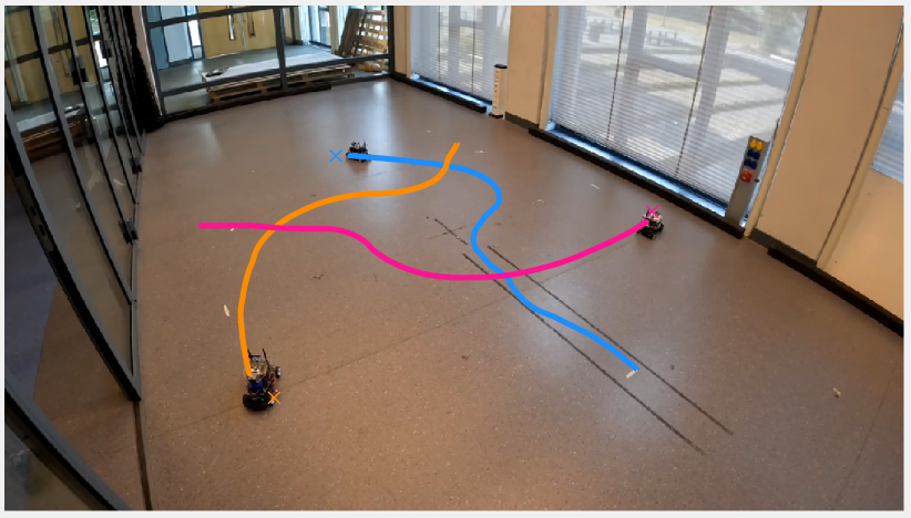
Figure 12: Experiments with $N=3$ car-like robots in a crossing circle scenario.

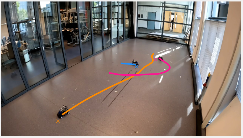
Figure 13: Experiments with $N=3$ car-like robots in a random room scenario.

RBL	$N$	$\eta$	max time (s)	mean speed (m/s)	RSR
circle ($3$ m)	3	0.0075	7.69	0.428	1.00
room ($5\times 3$ m2)	3	0.014	9.50	0.448	1.00

Table VIII: Quantitative experimental results for $N=3$ car-like robots in the crossing circle scenario and in the random room scenario (see Figure 12 and 13).

VI Conclusions

This paper provided two solutions for multi-robot motion planning and control, namely rule-based Lloyd (RBL) and Learning Lloyd-based (LLB) algorithm. Our solutions prove beneficial in a settings lacking of a centralized computational unit or a dependable communication network. In the case of RBL, we demonstrated both theoretically and through a comprehensive simulation campaign that each robot safely converges to its goal region. While through LLB, we showed that the Lloyd-based algorithm can be used as a safety-layer for learning-based algorithms. We believe that it can pave the way towards safe guaranteed learning-based algorithms and online learning as well. We provided also experimental results with $3$ car-like robots.

The main limitations of the proposed approach are the following: we can only guarantee to converge in a proximity of the goal position (see Proposition 1), the parameters have to be chosen carefully to meet the requirements for guarantee convergence (see Remark 1), and finally, we have to be aware that the numerical simulations give an approximation of the centroid position. To obtain a better approximation we have to pay in computational efficiency (by decreasing d$x$).

In the future, our objectives include addressing the mentioned limitations. Moreover, we plan to do experiments with more robots, possibly heterogeneous, including also non/partially-cooperative agents in the mission space (i.e., human beings).

Manuel Boldrer received the master’s degree in Mechatronic Engineering and Ph.D degree in Materials, Mechatronics and Systems Engineering from the University of Trento, Trento, Italy, respectively in 2018 and 2022. He was a Visiting Scholar at the University of California, Riverside, Riverside, US, in 2021. As of today, he is a Postdoctoral Researcher with the Cognitive Robotics Department (CoR), Delft University of Technology, Delft, The Netherlands, in the Reliable Robot Control Lab. His research interests include mobile robotics, distributed control and multi-agent systems.

Álvaro Serra-Gómez is a Ph.D. student at the Department of Cognitive Robotics at the Delft University of Technology. He received his M.Sc. (2019) both at the Polytechnic University of Catalonia in Automatic Control and Robotics and at the Ècole Polytechnique de Paris in Data Science in the Computer Science and Applied Mathematics Departments. His current research focuses on learning hierarchical motion planning policies to coordinate multi-robot systems in active perception and collision avoidance tasks.

Lorenzo Lyons received the M.Sc. degree in mechanical engineering from the Polytechnic University of Milan, Milan, Italy, in 2021. He is currently pursuing the Ph.D. degree with the Cognitive Robotics (CoR) Department, Delft University of Technology, Delft, The Netherlands. His research interests include numerical optimization, model predictive control, multi-robot motion planning applied to the automotive, and robotics.

Javier Alonso-Mora received the Ph.D. degree in robotics on cooperative motion planning from ETH Zurich, Zurich, Switzerland, in partnership with Disney Research Studios, Zurich, Switzerland. He is currently an Associate Professor with the Delft University of Technology, Delft, The Netherlands, where he leads the Autonomous Multi-robots Lab. He was a Postdoctoral Associate at the Computer Science and Artificial Intelligence Lab (CSAIL), Massachusetts Institute of Technology, Cambridge, MA, USA. His research interests include navigation, motion planning, and control of autonomous mobile robots, with a special emphasis on multirobot systems, mobile manipulation, ondemand transportation, and robots that interact with other robots and humans in dynamic and uncertain environments. Dr. Alonso-Mora is an Associate Editor for IEEE TRANSACTIONS ON ROBOTICS and for Springer Autonomous Robots. He was the recipient of a talent scheme VENI Award from the Netherlands Organization for Scientific Research (2017), ICRA Best Paper Award on Multi-robot Systems (2019), and an ERC Starting Grant (2021)

Laura Ferranti received the Ph.D. degree from the Delft University of Technology, Delft, The Netherlands, in 2017. She is currently an Assistant Professor with the Cognitive Robotics (CoR) Department, Delft University of Technology. Her research interests include optimization and optimal control, model predictive control, reinforcement learning, embedded optimization-based control with application in flight control, maritime transportation, robotics, and automotive. Dr. Ferranti was a recipient of the NWO Veni Grant from the Netherlands Organization for Scientific Research in 2020 and the Best Paper Award on Multi-Robot Systems at International Conference on Robotics and Automation (ICRA) 2019

References

- [1] G. Sharon, R. Stern, A. Felner, and N. R. Sturtevant, “Conflict-based search for optimal multi-agent pathfinding,” Artificial Intelligence, vol. 219, pp. 40–66, 2015.
- [2] J. Li, A. Tinka, S. Kiesel, J. W. Durham, T. S. Kumar, and S. Koenig, “Lifelong multi-agent path finding in large-scale warehouses,” in Proceedings of the AAAI Conference on Artificial Intelligence, vol. 35, no. 13, 2021, pp. 11 272–11 281.
- [3] J. Cheng, H. Cheng, M. Q.-H. Meng, and H. Zhang, “Autonomous navigation by mobile robots in human environments: A survey,” in 2018 IEEE international conference on robotics and biomimetics (ROBIO). IEEE, 2018, pp. 1981–1986.
- [4] J. Van den Berg, M. Lin, and D. Manocha, “Reciprocal velocity obstacles for real-time multi-agent navigation,” in 2008 IEEE international conference on robotics and automation. Ieee, 2008, pp. 1928–1935.
- [5] J. Van Den Berg, S. J. Guy, M. Lin, and D. Manocha, “Reciprocal n-body collision avoidance,” in Robotics Research: The 14th International Symposium ISRR. Springer, 2011, pp. 3–19.
- [6] J. Alonso-Mora, A. Breitenmoser, M. Rufli, P. Beardsley, and R. Siegwart, “Optimal reciprocal collision avoidance for multiple non-holonomic robots,” in Distributed Autonomous Robotic Systems: The 10th International Symposium. Springer, 2013, pp. 203–216.
- [7] M. Boldrer, L. Palopoli, and D. Fontanelli, “Socially-aware multi-agent velocity obstacle based navigation for nonholonomic vehicles,” in 2020 IEEE 44th Annual Computers, Software, and Applications Conference (COMPSAC). IEEE, 2020, pp. 18–25.
- [8] S. H. Arul and D. Manocha, “V-rvo: Decentralized multi-agent collision avoidance using voronoi diagrams and reciprocal velocity obstacles,” in 2021 IEEE/RSJ International Conference on Intelligent Robots and Systems (IROS). IEEE, 2021, pp. 8097–8104.
- [9] J. Godoy, S. J. Guy, M. Gini, and I. Karamouzas, “C-nav: Distributed coordination in crowded multi-agent navigation,” Robotics and Autonomous Systems, vol. 133, p. 103631, 2020.
- [10] A. Giese, D. Latypov, and N. M. Amato, “Reciprocally-rotating velocity obstacles,” in 2014 IEEE International Conference on Robotics and Automation (ICRA). IEEE, 2014, pp. 3234–3241.
- [11] D. Helbing and P. Molnar, “Social force model for pedestrian dynamics,” Physical review E, vol. 51, no. 5, p. 4282, 1995.
- [12] M. Boldrer, M. Andreetto, S. Divan, L. Palopoli, and D. Fontanelli, “Socially-aware reactive obstacle avoidance strategy based on limit cycle,” IEEE Robotics and Automation Letters, vol. 5, no. 2, pp. 3251–3258, 2020.
- [13] R. Gayle, W. Moss, M. C. Lin, and D. Manocha, “Multi-robot coordination using generalized social potential fields,” in 2009 IEEE International Conference on Robotics and Automation. IEEE, 2009, pp. 106–113.
- [14] L. Wang, A. D. Ames, and M. Egerstedt, “Safety barrier certificates for collisions-free multirobot systems,” IEEE Transactions on Robotics, vol. 33, no. 3, pp. 661–674, 2017.
- [15] F. Celi, L. Wang, L. Pallottino, and M. Egerstedt, “Deconfliction of motion paths with traffic inspired rules,” IEEE Robotics and Automation Letters, vol. 4, no. 2, pp. 2227–2234, 2019.
- [16] D. Fox, W. Burgard, and S. Thrun, “The dynamic window approach to collision avoidance,” IEEE Robotics & Automation Magazine, vol. 4, no. 1, pp. 23–33, 1997.
- [17] L. Ferranti, L. Lyons, R. R. Negenborn, T. Keviczky, and J. Alonso-Mora, “Distributed nonlinear trajectory optimization for multi-robot motion planning,” IEEE Transactions on Control Systems Technology, 2022.
- [18] A. Tajbakhsh, L. T. Biegler, and A. M. Johnson, “Conflict-based model predictive control for scalable multi-robot motion planning,” arXiv preprint arXiv:2303.01619, 2023.
- [19] H. Zhu and J. Alonso-Mora, “Chance-constrained collision avoidance for mavs in dynamic environments,” IEEE Robotics and Automation Letters, vol. 4, no. 2, pp. 776–783, 2019.
- [20] S. H. Arul, J. J. Park, and D. Manocha, “Ds-mpepc: Safe and deadlock-avoiding robot navigation in cluttered dynamic scenes,” arXiv preprint arXiv:2303.10133, 2023.
- [21] C. E. Luis and A. P. Schoellig, “Trajectory generation for multiagent point-to-point transitions via distributed model predictive control,” IEEE Robotics and Automation Letters, vol. 4, no. 2, pp. 375–382, 2019.
- [22] M. Kloock and B. Alrifaee, “Coordinated cooperative distributed decision-making using synchronization of local plans,” IEEE Transactions on Intelligent Vehicles, vol. 8, no. 2, pp. 1292–1306, 2023.
- [23] Y. Chen, C. Wang, M. Guo, and Z. Li, “Multi-robot trajectory planning with feasibility guarantee and deadlock resolution: An obstacle-dense environment,” IEEE Robotics and Automation Letters, vol. 8, no. 4, pp. 2197–2204, 2023.
- [24] Y. M. Chung, H. Youssef, and M. Roidl, “Distributed timed elastic band (dteb) planner: Trajectory sharing and collision prediction for multi-robot systems,” in 2022 International Conference on Robotics and Automation (ICRA). IEEE, 2022, pp. 10 702–10 708.
- [25] D. Zhou, Z. Wang, S. Bandyopadhyay, and M. Schwager, “Fast, on-line collision avoidance for dynamic vehicles using buffered voronoi cells,” IEEE Robotics and Automation Letters, vol. 2, no. 2, pp. 1047–1054, 2017.
- [26] H. Zhu and J. Alonso-Mora, “B-uavc: Buffered uncertainty-aware voronoi cells for probabilistic multi-robot collision avoidance,” in 2019 international symposium on multi-robot and multi-agent systems (MRS). IEEE, 2019, pp. 162–168.
- [27] M. Abdullhak and A. Vardy, “Deadlock prediction and recovery for distributed collision avoidance with buffered voronoi cells,” in 2021 IEEE/RSJ International Conference on Intelligent Robots and Systems (IROS). IEEE, 2021, pp. 429–436.
- [28] J.-L. Bastarache, C. Nielsen, and S. L. Smith, “On legible and predictable robot navigation in multi-agent environments,” in 2023 IEEE international conference on robotics and automation (ICRA). IEEE, 2023, pp. 5508–5514.
- [29] C. I. Mavrogiannis and R. A. Knepper, “Multi-agent path topology in support of socially competent navigation planning,” The International Journal of Robotics Research, vol. 38, no. 2-3, pp. 338–356, 2019.
- [30] B. Şenbaşlar, W. Hönig, and N. Ayanian, “Rlss: real-time, decentralized, cooperative, networkless multi-robot trajectory planning using linear spatial separations,” Autonomous Robots, pp. 1–26, 2023.
- [31] J. Park, I. Jang, and H. J. Kim, “Decentralized deadlock-free trajectory planning for quadrotor swarm in obstacle-rich environments–extended version,” arXiv preprint arXiv:2209.09447, 2022.
- [32] A. Patwardhan, R. Murai, and A. J. Davison, “Distributing collaborative multi-robot planning with gaussian belief propagation,” IEEE Robotics and Automation Letters, vol. 8, no. 2, pp. 552–559, 2023.
- [33] M. Čáp, J. Vokřínek, and A. Kleiner, “Complete decentralized method for on-line multi-robot trajectory planning in well-formed infrastructures,” in Proceedings of the international conference on automated planning and scheduling, vol. 25, 2015, pp. 324–332.
- [34] K. Kondo, J. Tordesillas, R. Figueroa, J. Rached, J. Merkel, P. C. Lusk, and J. P. How, “Robust mader: Decentralized and asynchronous multiagent trajectory planner robust to communication delay,” in 2023 IEEE International Conference on Robotics and Automation (ICRA). IEEE, 2023, pp. 1687–1693.
- [35] B. Şenbaşlar and G. S. Sukhatme, “Dream: Decentralized real-time asynchronous probabilistic trajectory planning for collision-free multi-robot navigation in cluttered environments,” arXiv preprint arXiv:2307.15887, 2023.
- [36] Y. Chen, M. Guo, and Z. Li, “Recursive feasibility and deadlock resolution in mpc-based multi-robot trajectory generation.” arXiv preprint arXiv:2202.06071, 2022.
- [37] Y. Chen, H. Dong, and Z. Li, “Asynchronous spatial allocation protocol for trajectory planning of heterogeneous multi-agent systems,” arXiv preprint arXiv:2309.07431, 2023.
- [38] J. Orr and A. Dutta, “Multi-agent deep reinforcement learning for multi-robot applications: A survey,” Sensors, vol. 23, no. 7, p. 3625, 2023.
- [39] Y. F. Chen, M. Liu, M. Everett, and J. P. How, “Decentralized non-communicating multiagent collision avoidance with deep reinforcement learning,” in 2017 IEEE international conference on robotics and automation (ICRA). IEEE, 2017, pp. 285–292.
- [40] Y. F. Chen, M. Everett, M. Liu, and J. P. How, “Socially aware motion planning with deep reinforcement learning,” in 2017 IEEE/RSJ International Conference on Intelligent Robots and Systems (IROS). IEEE, 2017, pp. 1343–1350.
- [41] R. Han, S. Chen, S. Wang, Z. Zhang, R. Gao, Q. Hao, and J. Pan, “Reinforcement learned distributed multi-robot navigation with reciprocal velocity obstacle shaped rewards,” IEEE Robotics and Automation Letters, vol. 7, no. 3, pp. 5896–5903, 2022.
- [42] Z. Xie and P. Dames, “Drl-vo: Learning to navigate through crowded dynamic scenes using velocity obstacles,” arXiv preprint arXiv:2301.06512, 2023.
- [43] R. Han, S. Chen, and Q. Hao, “Cooperative multi-robot navigation in dynamic environment with deep reinforcement learning,” in 2020 IEEE International Conference on Robotics and Automation (ICRA). IEEE, 2020, pp. 448–454.
- [44] T. Fan, P. Long, W. Liu, and J. Pan, “Distributed multi-robot collision avoidance via deep reinforcement learning for navigation in complex scenarios,” The International Journal of Robotics Research, vol. 39, no. 7, pp. 856–892, 2020.
- [45] Q. Tan, T. Fan, J. Pan, and D. Manocha, “Deepmnavigate: Deep reinforced multi-robot navigation unifying local & global collision avoidance,” in 2020 IEEE/RSJ International Conference on Intelligent Robots and Systems (IROS). IEEE, 2020, pp. 6952–6959.
- [46] P. Long, T. Fan, X. Liao, W. Liu, H. Zhang, and J. Pan, “Towards optimally decentralized multi-robot collision avoidance via deep reinforcement learning,” in 2018 IEEE international conference on robotics and automation (ICRA). IEEE, 2018, pp. 6252–6259.
- [47] B. Brito, M. Everett, J. P. How, and J. Alonso-Mora, “Where to go next: Learning a subgoal recommendation policy for navigation in dynamic environments,” IEEE Robotics and Automation Letters, vol. 6, no. 3, pp. 4616–4623, 2021.
- [48] C. Chen, Y. Liu, S. Kreiss, and A. Alahi, “Crowd-robot interaction: Crowd-aware robot navigation with attention-based deep reinforcement learning,” in 2019 international conference on robotics and automation (ICRA). IEEE, 2019, pp. 6015–6022.
- [49] M. Everett, Y. F. Chen, and J. P. How, “Motion planning among dynamic, decision-making agents with deep reinforcement learning,” in 2018 IEEE/RSJ International Conference on Intelligent Robots and Systems (IROS). IEEE, 2018, pp. 3052–3059.
- [50] J. Qin, J. Qin, J. Qiu, Q. Liu, M. Li, and Q. Ma, “Srl-orca: A socially aware multi-agent mapless navigation algorithm in complex dynamic scenes,” arXiv preprint arXiv:2306.10477, 2023.
- [51] Q. Li, F. Gama, A. Ribeiro, and A. Prorok, “Graph neural networks for decentralized multi-robot path planning,” in 2020 IEEE/RSJ International Conference on Intelligent Robots and Systems (IROS). IEEE, 2020, pp. 11 785–11 792.
- [52] J. Gielis, A. Shankar, and A. Prorok, “A critical review of communications in multi-robot systems,” Current Robotics Reports, vol. 3, no. 4, pp. 213–225, 2022.
- [53] M. Boldrer, L. Palopoli, and D. Fontanelli, “Lloyd-based approach for robots navigation in human-shared environments,” in 2020 IEEE/RSJ International Conference on Intelligent Robots and Systems (IROS). IEEE, 2020, pp. 6982–6989.
- [54] Á. Serra-Gómez, E. Montijano, W. Böhmer, and J. Alonso-Mora, “Active classification of moving targets with learned control policies,” IEEE Robotics and Automation Letters, vol. 8, no. 6, pp. 3717–3724, 2023.
- [55] S. Lloyd, “Least squares quantization in pcm,” IEEE transactions on information theory, vol. 28, no. 2, pp. 129–137, 1982.
- [56] J. Cortes, S. Martinez, T. Karatas, and F. Bullo, “Coverage control for mobile sensing networks,” IEEE Transactions on robotics and Automation, vol. 20, no. 2, pp. 243–255, 2004.
- [57] M. Boldrer, D. Fontanelli, and L. Palopoli, “Coverage control and distributed consensus-based estimation for mobile sensing networks in complex environments,” in 2019 IEEE 58th Conference on Decision and Control (CDC). IEEE, 2019, pp. 7838–7843.
- [58] M. Boldrer, P. Bevilacqua, L. Palopoli, and D. Fontanelli, “Graph connectivity control of a mobile robot network with mixed dynamic multi-tasks,” IEEE Robotics and Automation Letters, vol. 6, no. 2, pp. 1934–1941, 2021.
- [59] M. Boldrer, A. Antonucci, P. Bevilacqua, L. Palopoli, and D. Fontanelli, “Multi-agent navigation in human-shared environments: A safe and socially-aware approach,” Robotics and Autonomous Systems, vol. 149, p. 103979, 2022.
- [60] M. Boldrer, L. Palopoli, and D. Fontanelli, “A unified lloyd-based framework for multi-agent collective behaviours,” Robotics and Autonomous Systems, vol. 156, p. 104207, 2022.
- [61] J. Lee, Y. Lee, J. Kim, A. Kosiorek, S. Choi, and Y. W. Teh, “Set transformer: A framework for attention-based permutation-invariant neural networks,” in Int. Conf. on Mach. Learn., 2019, pp. 3744–3753.
- [62] J. Schulman, F. Wolski, P. Dhariwal, A. Radford, and O. Klimov, “Proximal policy optimization algorithms,” ArXiv, vol. abs/1707.06347, 2017.
- [63] E. Liang et al., “RLlib: Abstractions for distributed reinforcement learning,” in Int. Conf. on Mach. Lear., 2018.
- [64] T. Haarnoja, H. Tang, P. Abbeel, and S. Levine, “Reinforcement learning with deep energy-based policies,” in Proceedings of the 34th International Conference on Machine Learning (ICML), 2017.
- [65] R. S. Sutton and A. G. Barto, Reinforcement learning: An introduction. MIT press, 2018.
- [66] H. Zhu, B. Brito, and J. Alonso-Mora, “Decentralized probabilistic multi-robot collision avoidance using buffered uncertainty-aware voronoi cells,” Autonomous Robots, vol. 46, no. 2, pp. 401–420, 2022.
- [67] A. Zanelli, A. Domahidi, J. Jerez, and M. Morari, “Forces nlp: an efficient implementation of interior-point… methods for multistage nonlinear nonconvex programs,” International Journal of Control, pp. 1–17, 2017.
- [68] A. Domahidi and J. Jerez, “Forces professional,” Embotech AG, url=https://embotech.com/FORCES-Pro, 2014–2019.
- [69] M. Boldrer, A. Serra-Gómez, L. Lyons, J. Alonso-Mora, and L. Ferranti. Video associated with the submission. Youtube. [Online]. Available: https://youtu.be/ZCm-KYHxNG4
- [70] J. van den Berg, S. J. Guy, J. Snape, M. C. Lin, and D. Manocha, “Rvo2 library: Reciprocal collision avoidance for real-time multi-agent simulation,” See https://gamma. cs. unc. edu/RVO2, 2011.
- [71] C. E. Luis, M. Vukosavljev, and A. P. Schoellig, “Online trajectory generation with distributed model predictive control for multi-robot motion planning,” IEEE Robotics and Automation Letters, vol. 5, no. 2, pp. 604–611, 2020.
- [72] J. Park, D. Kim, G. C. Kim, D. Oh, and H. J. Kim, “Online distributed trajectory planning for quadrotor swarm with feasibility guarantee using linear safe corridor,” IEEE Robotics and Automation Letters, vol. 7, no. 2, pp. 4869–4876, 2022.