The Power of Explainability in Forecast-Informed Deep Learning Models for Flood Mitigation

Abstract

Floods can cause horrific harm to life and property. However, they can be mitigated or even avoided by the effective use of hydraulic structures such as dams, gates, and pumps. By pre-releasing water via these structures in advance of extreme weather events, water levels are sufficiently lowered to prevent floods. In this work, we propose FIDLAr, a Forecast Informed Deep Learning Architecture, achieving flood management in watersheds with hydraulic structures in an optimal manner by balancing out flood mitigation and unnecessary wastage of water via pre-releases. We perform experiments with FIDLAr using data from the South Florida Water Management District, which manages a coastal area that is highly prone to frequent storms and floods. Results show that FIDLAr performs better than the current state-of-the-art with several orders of magnitude speedup and with provably better pre-release schedules. The dramatic speedups make it possible for FIDLAr to be used for real-time flood management. The main contribution of this paper is the effective use of tools for model explainability, allowing us to understand the contribution of the various environmental factors towards its decisions.

1 Introduction

Floods can result in catastrophic loss of life jonkman2008loss , huge socio-economic impact wu2021new , property damage brody2007rising , and environmental devastation yin2023flash . While flood risks may be on the rise in both frequency and scale because of global climate changewing2022inequitable ; hirabayashi2013global , the resulting sea-level rise in coastal areas sadler2020exploring amplify the threats posed by floods. Therefore, improved and real-time flood management is of utmost significance. Managing the control schedules of hydraulic structures, such as dams, gates, pumps, and reservoirs kerkez2016smarter can make controlled flood mitigation possible bowes2021flood .

Currently, decades of human experience on specific river systems have resulted in rule-based methods bowes2021flood ; sadler2019leveraging to decide control schedules. However, the lack of sufficient experience to deal with extreme events leaves us vulnerable to catastrophic floods. Additionally, the schedules may not generalize to complex river systems schwanenberg2015open . Soft optimization methods and other physics-based models, which are currently used, are prohibitively slow leon2020matlab ; sadler2019leveraging ; vermuyten2018combining ; chen2016dimension ; leon2014dynamic .

Machine learning (ML) has emerged as a powerful approach for this domain willard2023time . Although ML-based methods have been used for flood prediction mosavi2018flood ; shi2023deep , flood detection tanim2022flood ; shahabi2020flood , susceptibility assessment saha2021flood ; islam2021flood , and post-flood management munawar2019after , they have not been used for flood mitigation. In this paper, we address this gap by applying well-engineered ML methods to the flood mitigation problem. FIDLAr, a Forecast Informed Deep Learning Architecture, is trained to mitigate floods after learning from historical observed data.

FIDLAr consists of two deep learning components. The Flood Manager predicts control schedules, while the Flood Evaluator validates the above output by predicting the water levels resulting from these schedules. FIDLAr has the following characteristics: (a) FIDLAr makes effective use of reliable forecasts of specific variables (e.g., precipitation and tidal information) for the near future shi2023explainable . (b) The training of FIDLAr is treated as an optimization problem where its output is optimized by minimizing a loss function with an eye toward balancing flood mitigation and water wastage. (c) During training, FIDLAr uses backpropagation from the Evaluator to improve the Manager by evaluating the generated schedules of the Manager. (d) FIDLAr outputs control schedules for the hydraulic structures in the river system (e.g., gates and pumps) so as to achieve effective flood mitigation. After pre-training with historical data, FIDLAr makes rapid predictions, achieving real-time flood mitigation.

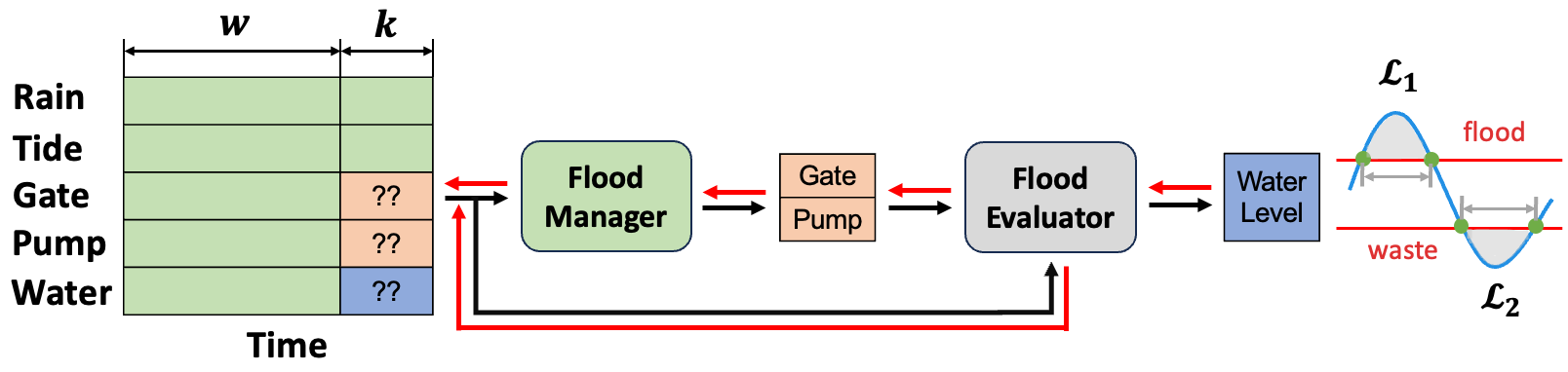
Figure 1: Forecast-Informed Deep Learning Architecture (FIDLAr). Input data in the form of a table consisting of five variables as shown in the left end of the diagram. The variables $w$ and $k$ are the lengths of the past and prediction windows, respectively. The parts of the table colored green are provided as inputs to the programs, while the orange and blue parts (with question marks) are outputs. The black and red arrows are the propagation and backpropagation processes. The Flood Manager and Flood Evaluator represent DL models, the former to predict the gate and pump schedules, and the latter to determine water levels for those schedules. Loss functions, $\mathcal{L}_{1}$ and $\mathcal{L}_{2}$, penalize the flooding and water wastage beyond thresholds, respectively.

2 Problem Formulation

Flood mitigation is achieved by predicting control schedules of hydraulic structures (gates and pumps) in the river system, $X^{gate,pump}_{t+1:t+k}$, for $k$ time points ($t+1$ through $t+k$) into the future, taking all the inputs, $X$, from the past $w$ time points, along with reliably forecasted covariates (rainfall and tide) for $k$ time points in the future. We train machine learning models to learn a function $f$ with parameters $\theta$ mapping the input variables to the control schedules. Thus,

$$f_{\theta}:(X_{t-w+1:t},X^{cov}_{t+1:t+k})\rightarrow X^{gate,pump}_{t+1:t+k},$$ (1)

where the subscripts represent the time ranges under consideration, and the superscripts refer to the covariates in question. If the covariates are not mentioned, then all the variables are being considered. The superscript $cov$ refers to the covariates, rain and tides, both of which can be reliably predicted.

3 Methodology

We trained the ML model to learn the function, $f_{\theta}$, by treating this as an optimization problem. During training, the Flood Manager generates a sequence of control schedules for the gates and pumps, which the Flood Evaluator is used to predict the resulting future water levels, $X^{water}_{t+1:t+k}$ (see Eq. (2)). The backpropagation algorithm lecun1988theoretical is used to backpropagate the feedback on the quality of the generated schedules (using loss functions, described in Section 3) to “nudge” the Flood Manager to produce more effective schedules. After the training of FIDLAr is completed, the Flood Evaluator does not perform backpropagation but provides validation for the schedules.

Flood Evaluator

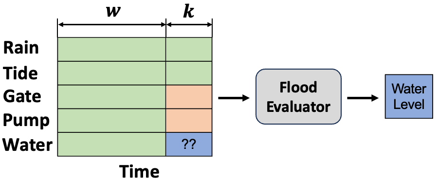
Figure 5: Flood Evaluator.

The Flood Evaluator is used to predict water levels at specific locations of interest along the river systems (see Fig. 5). Its transfer function is described below.

$$g_{\theta}:(X_{t-w+1:t},X^{cov}_{t+1:t+k},X^{gate,pump}_{t+1:t+k})\rightarrow X^{water}_{t+1:t+k}.$$ (2)

The Flood Evaluator is pre-trained to predict water levels as accurately as possible for different conditions and control schedules. Note that the parameters of the pre-trained Flood Evaluator are immutable either during the training or testing operation of FIDLAr. It merely plays the role of a trained “referee” to evaluate those generated control schedules in FIDLAr.

Flood Manager

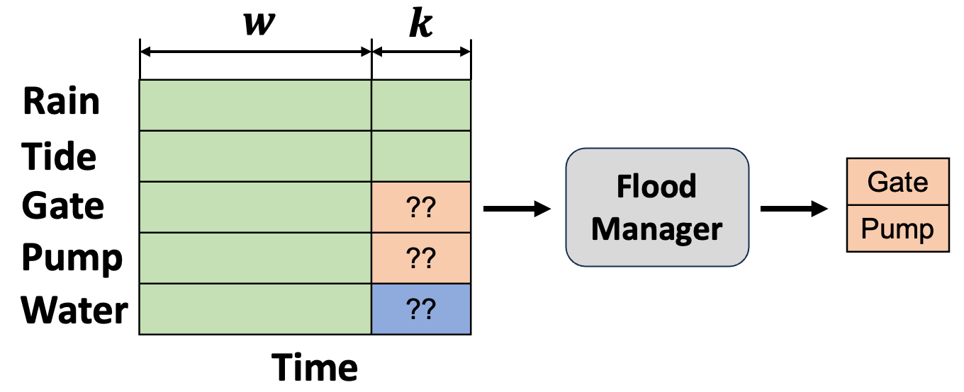
Figure 6: Flood Manager.

The Flood Manager is a DL-based model used to produce control schedules for hydraulic structures, taking reliably predictable future information (rain, tide) and all measured information from the recent past, as shown in Fig. 6. During training, the model parameters of Flood Manager are trained and optimized using the gradient descent algorithm with backpropagation from the Flood Evaluator ruder2016overview . The gradients are computed as partial derivatives of the loss functions (see Eq. (3) with respect to the input, i.e., green parts in Fig. 6).

Loss function

Loss functions are critical in steering the learning process to address the optimization goals. The metric of performance for the flood manager is the total time for which the water levels either exceed flooding threshold or dip below water wastage threshold. Another related metric is the extent to which the limits are exceeded to signify the severity of floods or water wastage.

$$\mathcal{L}_{1}=\sum^{N}_{i=1}\sum^{t+k}_{j=t+1}\Arrowvert max\{X^{water}_{i,j}-X^{flood}_{i},0\}\Arrowvert^{2},$$ (3)

$$\mathcal{L}_{2}=\sum^{N}_{i=1}\sum^{t+k}_{j=t+1}\Arrowvert min\{X^{water}_{i,j}-X^{waste}_{i},0\}\Arrowvert^{2},$$

where $N$ is the number of water level locations of interest; $k$ is the length of prediction horizon; $X^{flood}$ and $X^{waste}$ represent the thresholds for flooding and water wastage. The final loss function is a weighted combination of $\mathcal{L}_{1}$ and $\mathcal{L}_{2}$.

4 Experiments & Results

Flood Prediction

We compared eight DL models and one physics-based model (HEC-RAS) for the Flood Evaluator by predicting the water levels for a $k=24$-hour horizon. See Table 1 for the results.

Flood Mitigation

We tested eight DL models, two methods based on genetic algorithms (GA), and a rule-based baseline method, for flood mitigation. See Table 2 for the results.

5 Model Explainability

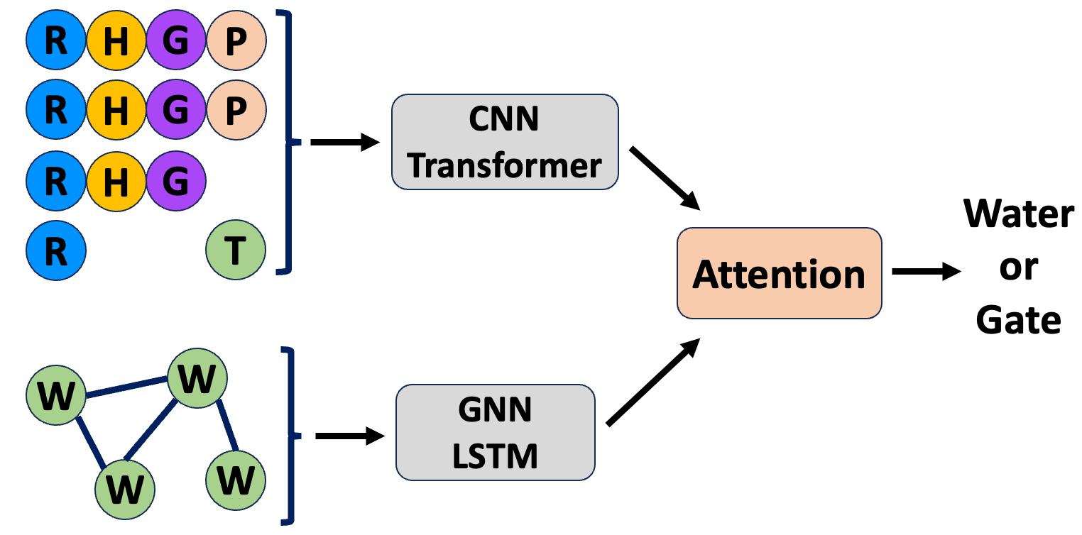
Figure 7: The Flood Graph Transformer Network (FloodGTN) model is assumed to have a collection of input variables, generically denoted by $R,T,G,P,H$, and $W$, measured at different measuring stations along the river system. The output variable is the set of water levels (for the Evaluator) or gate schedules (for the Manager).

To investigate the relationship between covariates and water levels of input variables, Fig. 2 visualizes the attention scores from the Attention layer vaswani2017attention of our FloodGTN model in Fig. 7. It reveals all water levels at key locations rely mainly on the tides (WS_S4). This makes sense when there are no structures between the location and the ocean. Besides, the water level at each location is also impacted by the structures close to it. These observations are consistent with prior knowledge.

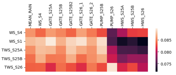
Figure 2: Attention scores between each variable of input. Labels such as S4, S1, S25A, S25B, S26 represent locations shown on the map of the S. Florida watershed in Fig. 4. WS_S4 represents the water level measured at location S4, which also corresponds to the tidal information.

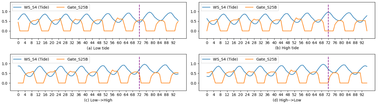
Figure 9: Visualization of input variables: WS_S4 (tide information) and Gate_S25B (gate schedules at location S25B). Time point 72 is NOW.

The contribution of each input variable (at each time point) on the model output was computed using LIME ribeiro2016should . Fig. 3 shows these contributions as heatmaps. First, what jumps out immediately is that the predicted water levels throughout the river system under normal conditions (mild to no rain) are overwhelmingly impacted by the tidal conditions measured at S4, which tend to be periodic. The impact of the nearby hydraulic structures is next in significance. Second, the highest contributions come from the covariates from the last 24 columns, which correspond to the future predicted tidal data, showing categorically that the future estimates for the 24-hour horizon are invaluable. The third critical insight is that FloodGTN focuses on the schedules of the gates, but only during low tide. This makes sense because water pre-releases must happen during low tides since releasing water is typically not possible during high tides. This was also confirmed by looking at the historical data (see Fig. 9). Finally, we observe that predicted water levels also depend on data from the near past (see Fig. 3(b)), and this dependence wanes as we consider variables from the more distant past.

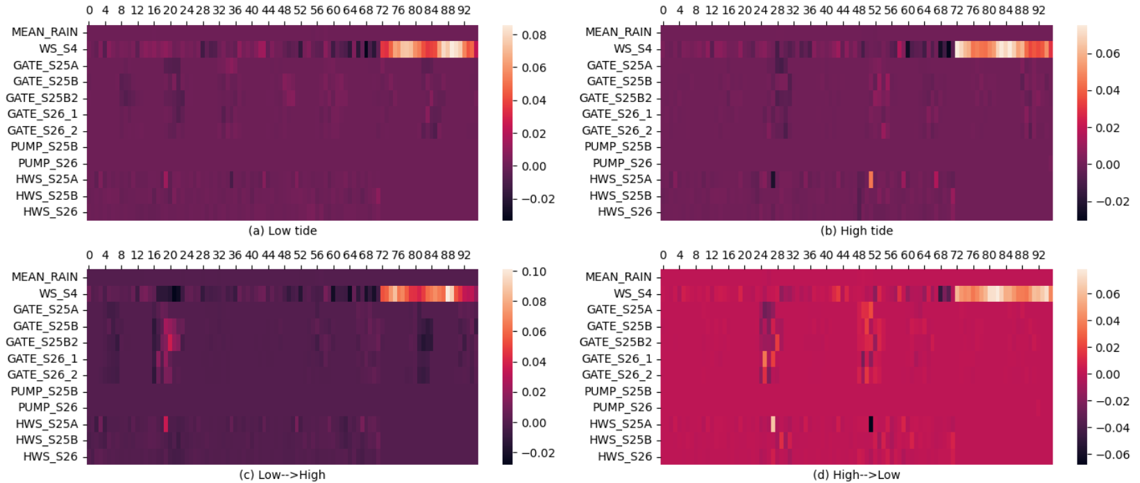
(a) Contribution of each covariate to predict water levels for the next 24 hours.

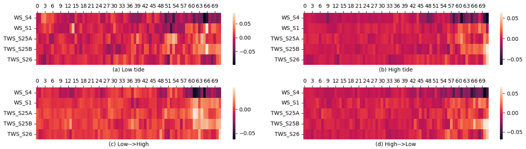
(b) Contribution of water level readings for the past 3 days to predict water levels for the next 24 hours.

Figure 3: Model explainability for the contribution of input to output. Time point 72 is NOW, which ends based on the water levels at (a) low tide, (b) high tide, (c) low to high, and (d) high to low.

6 Conclusions

FIDLAr is a DL-based tool to compute water “pre-release” schedules for hydraulic structures to achieve effective and efficient flood mitigation, while ensuring water wastage is avoided by managing the extent of pre-release. FIDLAr consists of two DL-based components (Flood Manager & Flood Evaluator). During training, backpropagation from the Evaluator helps or even forces the Manager to generate better outputs. Finally, we summarize that all the DL-based versions of FIDLAr are orders of magnitude faster than the (physics-based or GA-based) competitors, while achieving better flood mitigation. The use of explainability tools provides rare insights into a coastal system while validating DL models are learning correct and useful knowledge from the input.

Appendix A Dataset

We obtained data on a coastal section of the South Florida watershed from the South Florida Water Management District’s (SFWMD) DBHydro database. The data set we used in the work recorded the hourly observations for water levels and external covariates from 2010 to 2020. As shown in Figure 4, the river system has three branches/tributaries and includes several hydraulic structures – gates and pumps – located along the river system to control water flows. Water levels are also impacted by ocean tides since the river system empties itself into the ocean. In this work, we aim to predict the effective schedules of the gates and pumps to mitigate or avoid flooding at four specific locations marked by green circles in Fig. 4. It is useful to note that this portion of the river system flows through the large metropolis of Miami, which has a sizable population, commercial enterprises, and an international airport in its close vicinity.

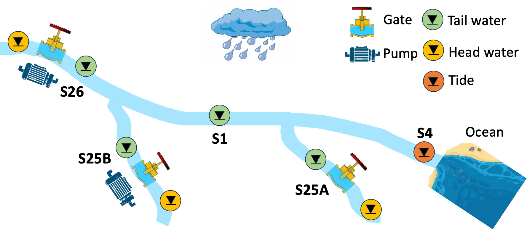
Figure 4: Schemetic diagram of the study domain - South Florida. There are three water stations with hydraulic structures (gates and pumps), one water station, and four control points of interest (labeled S1, S25A, S25B, S26 and marked with a green circle), and one station (S4) monitoring tidal information.

Appendix B Model details

B.1 Framework of Flood Evaluator and Flood Manager

The architecture of the Flood Evaluator and Flood Manager are described here. The Flood Evaluator is used to predict the water levels based on the input of past information of all variables and any future covariates that may be estimated in advance. The future tide and rain information could be reliably predicted, while gate and pump information are decided by the operators. After pre-training, the Flood Evaluator can play the role of "scorer" to evaluate the quality of gate and pump schedules. The Flood Manager is used to generate the gate and pump schedules given the input of past information of all variables and estimated future covariates (i.e., rain and tide information). Variables $w$ and $k$ represent the length of the past and future horizons, respectively.

B.2 FloodGTN

The best-performing DL model for Flood prediction and mitigation is described here and is referred to as FloodGTN (Graph Transformer Network). More specifically, FloodGTN combines graph neural networks (GNNs), attention-based transformer networks, long short-term memory networks (LSTMs), and convolutional neural networks (CNNs) for various objectives. The GNN-LSTM model learns the spatio-temporal dynamics of water levels, while the CNN-Transformer module learns feature representations from the inputs. Attention is used to figure out the interactions between covariates and water levels. This model works best for both the flood evaluator and the manager.

Appendix C Experimental results

C.1 Results for flood prediction

The table below compares the performance of a graph-transformer-based evaluator tool (labeled FloodGTN) with the ground truth (measured data), physics-based HEC-RAS model, and seven other DL models.

Methods	MAE (ft)	RMSE (ft)	OverTime	OverArea	UnderTime	UnderArea
Ground-truth	-	-	96	14.82	1,346	385.8
HEC-RAS	0.174	0.222	68	10.07	1,133	325.33
MLP	0.065	0.086	147	27.96	1,677	500.41
RNN	0.054	0.072	110	17.12	1,527	441.41
CNN	0.079	0.104	58	5.91	1,491	413.22
GNN	0.054	0.070	102	15.90	1,569	462.63
TCN	0.050	0.065	47	5.14	1,607	453.63
RCNN	0.092	0.110	37	4.61	1,829	553.20
Transformer	0.050	0.066	151	25.95	1,513	434.13
FloodGTN	0.040	0.056	100	15.64	1,764	549.28

Table 1: Comparison of different models for the Flood Evaluator on test set (at time t+1 for measuring station S1). OverTime (UnderTime) represents the number of time steps during which the water levels exceed the upper threshold (subceed the lower threshold). Similarly, OverArea (UnderArea) refers to the area between the water level curve and the upper threshold (lower threshold).

C.2 Results for flood mitigation

The table below compares the performance of FIDLAr (a graph-transformer-based flood mitigation tool using FloodGTN as an evaluator) with the rule-based method, two GA-based tools, and seven other DL models.

	Methods	OverTime	OverArea	UnderTime	UnderArea
	Rule-based	96	14.82	1,346	385.8
GA-Based	Genetic Algorithm∗	-	-	-	-
	Genetic Algorithm†	86	16.54	454	104
DL-Based	MLP	91	13.31	1,071	268.35
	RNN	35	3.97	251	41.05
	CNN	81	11.22	1,163	314.37
	GNN	31	3.72	429	84.31
	TCN	39	3.77	306	55.12
	RCNN	29	3.28	328	58.68
	Transformer	85	11.54	1,180	310.16
	FIDLAr/FloodGTN	22	2.23	299	53.34

Table 2: Comparison of the Flood Manager tool, FIDLAr on test set (at time t+1 for station S1). The GA method with a $*$ was used with a physics-based (HEC-RAS) as the Evaluator, while the GA method with a ${\dagger}$ was used with the DL-based FloodGTN as the Evaluator. All other rows are DL-based flood managers with FloodGTN as the Evaluator.

C.3 Results for flood mitigation for a small event at a certain location

Here we visualize the water levels with the rule-based and the DL-based approaches FIDLAr for a short sample for one location of interest in Figure 8. The zoomed portion shows a 2.5-hour period where the floods are mitigated to bring water levels to under 3.5 feet based on the predicted gate and pump schedules. The corresponding performance measures for this small sample are provided in Table 3.

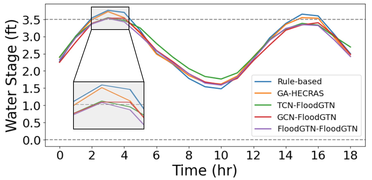
Figure 8: Flood mitigation visualization for a short sample spanning 18 hours from Sep. 3rd (09:00) to Sep. 4th (03:00) in 2019 for one location of interest. We zoomed in on the time period $t=2$ to 4.5 hours, shaded in gray.

Table 3 below shows the corresponding results for Fig. 8.

	Methods	Over Timesteps	Over Area
	Rule-based	6	0.866
GA-Based	Genetic Algorithm∗	4	0.351
	Genetic Algorithm†	6	0.764
DL-Based	MLP	6	0.614
	RNN	1	0.074
	CNN	6	0.592
	GNN	2	0.062
	TCN	1	0.046
	RCN	1	0.045
	Transformer	6	0.614
	FIDLAr/FloodGTN	1	0.022

Table 3: Comparison of different methods of Flood Manager for flood Mitigation (at time t+1 for one event S1). The experimental results correspond to the time period displayed in Fig. 8. The GA method with a $*$ was used with a physics-based (HEC-RAS) as the Evaluator, while the GA method with a ${\dagger}$ was used with the DL-based FloodGTN as the Evaluator. All other rows are DL-based flood managers with FloodGTN as the Evaluator.

C.4 Computational time

Table 4 shows the running times for all the methods for the evaluator component and for the whole flood mitigation system in its test phase. All the DL-based approaches are several orders of magnitude faster than the currently used physics-based and GA-based approaches. The table also shows the training times for the DL-based approaches, which do not impact the real-time performance, once deployed.

Model	Prediction		Mitigation
	Train	Test	Train	Test
HEC-RAS	-	45 min	-	-
Rule-based	-	-	-	-
GA∗	-	-	-	-
GA†	-	-	-	est. 30 h
MLP	35 min	1.88 s	58 min	6.13 s
RNN	243 min	8.57 s	54 min	12.75 s
CNN	37 min	1.93 s	17 min	5.84 s
GNN	64 min	3.13 s	29 min	7.26 s
TCN	60 min	4.57 s	45 min	9.06 s
RCNN	136 min	8.61 s	61 min	13.27 s
Transformer	43 min	2.38 s	23 min	6.76 s
FloodGTN	119 min	2.95 s	35 min	4.90 s

Table 4: The running times for flood prediction and mitigation. The running times for the rule-based method are not reported since historical data was directly used. GA^∗, which combines a GA-based tool and HEC-RAS, took too long and was not reported. GA^†, which combines the GA-based tool with FloodGTN, also took too long but was estimated using a smaller sample.

Appendix D Visualization of observed variables

We visualize the observed variables, WS_S4, Gate_S25B, for a better understanding of explainability in Fig. 3(a).

References

- [1] Benjamin D Bowes, Arash Tavakoli, Cheng Wang, Arsalan Heydarian, Madhur Behl, Peter A Beling, and Jonathan L Goodall. Flood mitigation in coastal urban catchments using real-time stormwater infrastructure control and reinforcement learning. Journal of Hydroinformatics, 23(3):529–547, 2021.
- [2] Samuel D Brody, Sammy Zahran, Praveen Maghelal, Himanshu Grover, and Wesley E Highfield. The rising costs of floods: Examining the impact of planning and development decisions on property damage in florida. Journal of the American Planning Association, 73(3):330–345, 2007.
- [3] Duan Chen, Arturo S Leon, Nathan L Gibson, and Parnian Hosseini. Dimension reduction of decision variables for multireservoir operation: A spectral optimization model. Water Resources Research, 52(1):36–51, 2016.
- [4] Yukiko Hirabayashi, Roobavannan Mahendran, Sujan Koirala, Lisako Konoshima, Dai Yamazaki, Satoshi Watanabe, Hyungjun Kim, and Shinjiro Kanae. Global flood risk under climate change. Nature climate change, 3(9):816–821, 2013.
- [5] Abu Reza Md Towfiqul Islam, Swapan Talukdar, Susanta Mahato, Sonali Kundu, Kutub Uddin Eibek, Quoc Bao Pham, Alban Kuriqi, and Nguyen Thi Thuy Linh. Flood susceptibility modelling using advanced ensemble machine learning models. Geoscience Frontiers, 12(3):101075, 2021.
- [6] Sebastiaan N Jonkman and Johannes K Vrijling. Loss of life due to floods. Journal of Flood Risk Management, 1(1):43–56, 2008.
- [7] Branko Kerkez, Cyndee Gruden, Matthew Lewis, Luis Montestruque, Marcus Quigley, Brandon Wong, Alex Bedig, Ruben Kertesz, Tim Braun, Owen Cadwalader, et al. Smarter stormwater systems, 2016.
- [8] Yann LeCun, D Touresky, G Hinton, and T Sejnowski. A theoretical framework for back-propagation. In Proceedings of the 1988 connectionist models summer school, volume 1, pages 21–28. San Mateo, CA, USA, 1988.
- [9] Arturo S Leon, Elizabeth A Kanashiro, Rachelle Valverde, and Venkataramana Sridhar. Dynamic framework for intelligent control of river flooding: Case study. Journal of Water Resources Planning and Management, 140(2):258–268, 2014.
- [10] Arturo S Leon, Yun Tang, Li Qin, and Duan Chen. A matlab framework for forecasting optimal flow releases in a multi-storage system for flood control. Environmental Modelling & Software, 125:104618, 2020.
- [11] Amir Mosavi, Pinar Ozturk, and Kwok-wing Chau. Flood prediction using machine learning models: Literature review. Water, 10(11):1536, 2018.
- [12] Hafiz Suliman Munawar, Ahmad Hammad, Fahim Ullah, and Tauha Hussain Ali. After the flood: A novel application of image processing and machine learning for post-flood disaster management. In Proceedings of the 2nd International Conference on Sustainable Development in Civil Engineering (ICSDC 2019), Jamshoro, Pakistan, pages 5–7, 2019.
- [13] Marco Tulio Ribeiro, Sameer Singh, and Carlos Guestrin. " why should i trust you?" explaining the predictions of any classifier. In Proceedings of the 22nd ACM SIGKDD international conference on knowledge discovery and data mining, pages 1135–1144, 2016.
- [14] Sebastian Ruder. An overview of gradient descent optimization algorithms. arXiv preprint arXiv:1609.04747, 2016.
- [15] Jeffrey M Sadler, Jonathan L Goodall, Madhur Behl, Benjamin D Bowes, and Mohamed M Morsy. Exploring real-time control of stormwater systems for mitigating flood risk due to sea level rise. Journal of Hydrology, 583:124571, 2020.
- [16] Jeffrey M Sadler, Jonathan L Goodall, Madhur Behl, Mohamed M Morsy, Teresa B Culver, and Benjamin D Bowes. Leveraging open source software and parallel computing for model predictive control of urban drainage systems using epa-swmm5. Environmental Modelling & Software, 120:104484, 2019.
- [17] Asish Saha, Subodh Chandra Pal, Alireza Arabameri, Thomas Blaschke, Somayeh Panahi, Indrajit Chowdhuri, Rabin Chakrabortty, Romulus Costache, and Aman Arora. Flood susceptibility assessment using novel ensemble of hyperpipes and support vector regression algorithms. Water, 13(2):241, 2021.
- [18] D Schwanenberg, BPJ Becker, and M Xu. The open real-time control (rtc)-tools software framework for modeling rtc in water resources sytems. Journal of Hydroinformatics, 17(1):130–148, 2015.
- [19] Himan Shahabi, Ataollah Shirzadi, Kayvan Ghaderi, Ebrahim Omidvar, Nadhir Al-Ansari, John J Clague, Marten Geertsema, Khabat Khosravi, Ata Amini, Sepideh Bahrami, et al. Flood detection and susceptibility mapping using sentinel-1 remote sensing data and a machine learning approach: Hybrid intelligence of bagging ensemble based on k-nearest neighbor classifier. Remote Sensing, 12(2):266, 2020.
- [20] Jimeng Shi, Rukmangadh Myana, Vitalii Stebliankin, Azam Shirali, and Giri Narasimhan. Explainable parallel rcnn with novel feature representation for time series forecasting. arXiv preprint arXiv:2305.04876, 2023.
- [21] Jimeng Shi, Zeda Yin, Rukmangadh Myana, Khandker Ishtiaq, Anupama John, Jayantha Obeysekera, Arturo Leon, and Giri Narasimhan. Deep learning models for water stage predictions in south florida. arXiv preprint arXiv:2306.15907, 2023.
- [22] Ahad Hasan Tanim, Callum Blake McRae, Hassan Tavakol-Davani, and Erfan Goharian. Flood detection in urban areas using satellite imagery and machine learning. Water, 14(7):1140, 2022.
- [23] Ashish Vaswani, Noam Shazeer, Niki Parmar, Jakob Uszkoreit, Llion Jones, Aidan N Gomez, Łukasz Kaiser, and Illia Polosukhin. Attention is all you need. Advances in neural information processing systems, 30, 2017.
- [24] Evert Vermuyten, Pieter Meert, Vincent Wolfs, and Patrick Willems. Combining model predictive control with a reduced genetic algorithm for real-time flood control. Journal of Water Resources Planning and Management, 144(2):04017083, 2018.
- [25] Jared D Willard, Charuleka Varadharajan, Xiaowei Jia, and Vipin Kumar. Time series predictions in unmonitored sites: A survey of machine learning techniques in water resources. arXiv preprint arXiv:2308.09766, 2023.
- [26] Oliver EJ Wing, William Lehman, Paul D Bates, Christopher C Sampson, Niall Quinn, Andrew M Smith, Jeffrey C Neal, Jeremy R Porter, and Carolyn Kousky. Inequitable patterns of us flood risk in the anthropocene. Nature Climate Change, 12(2):156–162, 2022.
- [27] Xianhua Wu, Ji Guo, Xianhua Wu, and Ji Guo. A new economic loss assessment system for urban severe rainfall and flooding disasters based on big data fusion. Economic impacts and emergency management of disasters in China, pages 259–287, 2021.
- [28] Jie Yin, Yao Gao, Ruishan Chen, Dapeng Yu, Robert Wilby, Nigel Wright, Yong Ge, Jeremy Bricker, Huili Gong, and Mingfu Guan. Flash floods: why are more of them devastating the world’s driest regions? Nature, 615(7951):212–215, 2023.