Industrial-Scale Mass Measurements of Isolated Black Holes

Abstract

I show that industrial-scale mass measurement of isolated black holes (BHs) can be achieved by combining a high-cadence, wide-field microlensing survey such as KMTNet, observations from a parallax satellite in solar orbit, and VLTI GRAVITY+ interferometry. I show that these can yield precision measurements of microlens parallaxes down to $\pi_{\rm E}\sim 0.01$ and Einstein radii down to $\theta_{\rm E}\sim 1\,{\rm mas}$. These limits correspond to BH masses $M\sim 12\,M_{\odot}$, deep in the Galactic bulge, with lens-source separations of $D_{LS}\sim 0.6\,$kpc, and they include all BHs in the Galactic disk. I carry out detailed analyses of simulations that explore many aspects of the measurement process, including the decisions on whether to carry out VLTI measurements for each long-event candidate. I show that the combination of ground-based and space-based light curves of BH events will automatically exclude the spurious “large parallax” solutions that arise from the standard (Refsdal, 1966) analysis, except for the high-magnification events, for which other methods can be applied. The remaining two-fold degeneracy can always be broken by conducting a second VLTI measurement, and I show how to identify the relatively rare cases that this is required.

1 Introduction

Microlensing is the only known method to measure the masses of isolated dark objects, in particular isolated black holes (BHs). Such measurements require the determination of two parameters that are not returned by standard (Paczyński, 1986) fits to the microlensing light curve, i.e., the Einstein radius, $\theta_{\rm E}$, and the microlens parallax ${\mbox{\boldmath$\pi$}}_{\rm E}$,

$$\theta_{\rm E}\equiv\sqrt{\kappa M\pi_{\rm rel}},\qquad{\mbox{\boldmath$\pi$}}_{\rm E}\equiv{\pi_{\rm rel}\over\theta_{\rm E}}{{\mbox{\boldmath$\mu$}}_{\rm rel}\over\mu_{\rm rel}};\qquad\kappa\equiv{4G\over c^{2}{\rm au}}=8.14\,{{\rm mas}\over M_{\odot}}.$$ (1)

Here, $M$ is the lens mass while $\pi_{\rm rel}$ and ${\mbox{\boldmath$\mu$}}_{\rm rel}$ are the lens-source relative parallax and proper-motion. Thus (Gould, 1992, 2000),

$$M={\theta_{\rm E}\over\kappa\pi_{\rm E}},$$ (2)

where $\pi_{\rm E}=|{\mbox{\boldmath$\pi$}}_{\rm E}|$.

However, although this principle has been known for three decades, to date, there has been only one isolated BH mass measurement (Sahu et al., 2022; Lam et al., 2022; Mróz et al., 2022), despite the fact that of order 1% of the $\sim 3\times 10^{4}$ known microlensing events are likely due to BHs. The main problem is that for dark objects, measurements of $\theta_{\rm E}$ and ${\mbox{\boldmath$\pi$}}_{\rm E}$ are each rare, so that their overlap is extremely rare. See Gould et al. (2023) for a systematic discussion.

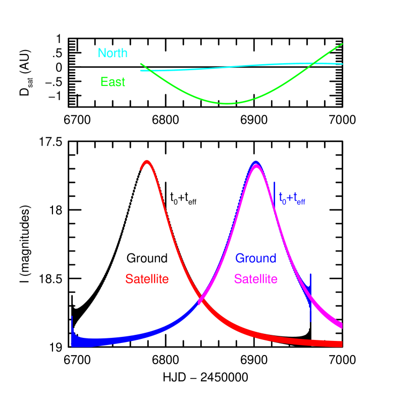
Figure 1: Light curves for simulated Events 1 (left) and 2 (right). The ground data are shown, respectively, in black and blue, while the satellite data are shown in red and magenta. The ground data are binned by day, based on the mean number of observations expected as a function of time of year. The north and east components of the Earth-satellite distance ${\bf D}_{\rm sat}$ are shown in the upper panel for the epochs when data can be taken. That is, the epochs when the satellite would be pointed $<45^{\circ}$ from the Sun are excluded.

For such isolated dark objects, there are two established methods to measure ${\mbox{\boldmath$\pi$}}_{\rm E}$ and three established methods to measure $\theta_{\rm E}$. In brief, ${\mbox{\boldmath$\pi$}}_{\rm E}$ can be measured either by observing the event from a single site on an accelerated platform (Gould, 1992) or by simultaneous observations from two well-separated observatories (Refsdal, 1966). Of course, almost all microlensing events are observed from Earth, which is an accelerated platform, whose parallactic motion induces annual bumps in the light curve, with an amplitude that is proportional to $\pi_{\rm E}$ and a phase that reflects the direction of ${\mbox{\boldmath$\mu$}}_{\rm rel}$. However, as most events are short compared to a year, it is generally difficult to extract ${\mbox{\boldmath$\pi$}}_{\rm E}$. See Figure 1 of Gould & Horne (2013). While BHs tend to have longer timescales $t_{\rm E}=\theta_{\rm E}/\mu_{\rm rel}$ (because $\theta_{\rm E}\propto M^{1/2}$), typical BH events are still short compared to a year. Moreover, typical BHs have small $\pi_{\rm E}\propto M^{-1/2}$. For example, it is likely that more than half of BH events are due to bulge BHs, which have $\pi_{\rm rel}\sim{\cal O}(15\,\mu{\rm as})$, so that an $M=10\,M_{\odot}$ BH would have $\pi_{\rm E}\sim 0.014$. Hence, a $5\,\sigma$ (20%) measurement would require $\sigma(\pi_{\rm E})=0.003$, which (for typical proper motions, $\mu_{\rm rel}\sim 6\,{\rm mas}\,{\rm yr}^{-1}$, i.e., $t_{\rm E}=\theta_{\rm E}/\mu_{\rm rel}=\kappa M\pi_{\rm E}/\mu_{\rm rel}\sim 70\,$days), are extremely rare. Moreover, systematic errors due to unmodeled instrumental effects in the light curve are believed to be significantly larger than this threshold. In particular, the one measured BH, OGLE-2011-BLG-0462, lies far in the opposite extreme of parameters space, a very rare event with $\pi_{\rm rel}\sim 0.5\,{\rm mas}$.

Hence, if it can be made into a practical option, the other approach, i.e., observations by a second observatory would be much preferred. In this case, the parallax is given approximately by

$${\mbox{\boldmath$\pi$}}_{\rm E}={{\rm au}\over D_{\perp}}\biggl{(}{\Delta t_{0}\over t_{\rm E}},\Delta u_{0}\biggr{)}$$ (3)

where ${\bf D}_{\perp}$ is the vector separation of the two observatories, $\Delta t_{0}$ is the difference of times of peak ($t_{0}$) between these observatories, and $\Delta u_{0}$ is their difference of impact parameters ($u_{0}$) normalized to $\theta_{\rm E}$. The two components are in the directions parallel and perpendicular to ${\bf D}_{\perp}$. As already recognized by Refsdal (1966), Equation (3) has a 4-fold ambiguity because $u_{0}$ is a signed quantity, but only its amplitude is typically measured from Paczyński (1986) fits to the light curve. See Figure 1 from Gould (1994b). This can be a serious issue, but I defer discussion of it to the exposition of the method that I propose. I should also mention (but also defer discussion of) another issue that impacts this measurement via the second component of Equation (3): it is subject to much larger statistical errors than the first component (Gould, 1995), as well as much larger systematic errors. In addition, for the most practical implementation of this idea, i.e., a satellite in solar orbit with $D_{\perp}\sim 1\,{\rm au}$, and for bulge lenses, the typical values of the two components will be small, $|\Delta t_{0}/t_{\rm E}|\lesssim 0.01$ and $|\Delta u_{0}|\lesssim 0.01$, so that control of statistical and systematic errors can be a major issue.

By far, the most common method to measure $\theta_{\rm E}$ for isolated objects, including dark ones, has been from so-called “finite-source” (FS) effects for the special case that the lens transits the source (Gould, 1994a; Witt & Mao, 1994; Nemiroff & Wickramasinghe, 1994). This includes the first isolated dark-object mass measurement, OGLE-2007-BLG-0224 (Gould et al., 2009), which was a brown dwarf (BD, Shan et al. 2021). Indeed, of the 30 $\theta_{\rm E}$ measurements of isolated objects with giant-star sources from the systematic study by Gould et al. (2022), of order 1/3 were dark, including four free-floating planet (FFP) candidates and of order six or more BDs. However, for the same reason that this is a powerful method for $\theta_{\rm E}$ measurements of low-mass dark objects, it is almost useless for BHs. That is, the probability of such transits is $p\simeq{\rm min}(1,\rho)$, where $\rho\equiv\theta_{*}/\theta_{\rm E}$ and $\theta_{*}$ is the angular radius of the source. Hence, of the several hundred isolated-BH events that have likely occurred, we expect less than one to have shown FS effects.

A second method to measure $\theta_{\rm E}$ is astrometric microlensing (Walker, 1995; Hog et al., 1995; Miyamoto & Yoshii, 1995), and indeed this was the method applied for the only isolated BH mass measurement, i.e., of OGLE-2011-BLG-0462. The method relies on the fact that the centroid of light from the two microlensed images is displaced from the source by

$$\Delta{\mbox{\boldmath$\theta$}}_{\rm cent}={{\bf u}\over u^{2}+2}\theta_{\rm E},$$ (4)

where ${\bf u}$ is the vector separation of the source relative to the lens, normalized to $\theta_{\rm E}$. In particular, the amplitude $u=|{\bf u}|$ is known from the instantaneous magnification $A=(u^{2}+2)/(u\sqrt{u^{2}+4})$ (Einstein, 1936), i.e., $u^{2}=2[(1-1/A^{2})^{-1/2}-1]$. After the source proper motion ${\mbox{\boldmath$\mu$}}_{S}$ is measured from late-time astrometric observations and is subtracted out, the light centroid traces an ellipse whose semi-major axis is $\theta_{a}=\theta_{\rm E}/\sqrt{8}$ (provided that $u_{0}\leq\sqrt{2}$). This method is challenging, in part because the observations must be carried out for many $t_{\rm E}$ in order to measure ${\mbox{\boldmath$\mu$}}_{S}$, and in part because the amplitude of the effect is small given present astrometric technology at the relatively faint magnitudes of typical microlensing events. That is, as mentioned above, typical bulge BHs have $\theta_{\rm E}=\kappa M\pi_{\rm E}\sim 1.1\,{\rm mas}$, implying $\theta_{a}\sim 300\,\mu{\rm as}$. Hence, a 20% measurement would require an error of just $\sigma(\theta_{a})\sim 60\,\mu{\rm as}$. In fact, the $\sim 10\%$ measurement of $\theta_{\rm E}$ for the case of OGLE-2011-BLG-0462 was only possible because $\theta_{\rm E}\sim 5.6\,{\rm mas}$ was exceptionally large, which again was due to fact that the BH was unusually close to the Sun. Thus, with present technology, this technique cannot be reliably applied to bulge BHs and presents considerable challenges for typical disk BHs, which have $\theta_{\rm E}\lesssim 2\,{\rm mas}$.

The third method is to resolve the two microlensed images using interferometry (Delplancke et al., 2001; Dong et al., 2019; Cassan et al., 2021). Their separation is given by

$$\Delta{\mbox{\boldmath$\theta$}}_{-,+}=2\sqrt{1+{u^{2}\over 4}}\theta_{\rm E}{\bf\hat{u}},$$ (5)

Note that the square-root term is very nearly unity, i.e., $\sim 1+u^{2}/8$, and in any case is known very precisely. Hence, if this method can be applied at all, it gives extremely precise determinations of $\theta_{\rm E}$. There are three restrictions on such applications, one of principle and the other two practical. The restriction of principle is that for any given baseline configuration of the interferometer, there is a threshold of detection. For the only interferometer capable of reaching typical microlensing events, i.e., the Very Large Telescope Interferometer (VLTI), this threshold is separations of about 2 mas, i.e., $\theta_{\rm E}\gtrsim 1\,{\rm mas}$. Fortunately, this threshold allows measurements for essentially all disk BHs and for half or more of bulge BHs.

The first practical consideration is that the sensitivity of the VLTI depends critically on engineering issues. Hence, for the original VLTI GRAVITY instrument (GRAVITY Collaboration et al., 2017), only targets that are much brighter than typical microlensing events were accessible. This is the reason that the first successful resolution of microlensed images was for an event that was several hundred times brighter than typical (Dong et al., 2019). However, with the advent of “GRAVITY Wide” (GRAVITY Wide Collaboration et al., 2022), of order 10% of microlensing events are already accessible. Moreover, a future upgrade to “GRAVITY+” (GRAVITY+ Collaboration et al., 2022) is already in progress, after which the bulk of microlensing events will be accessible.

The second practical consideration is that observing time must be allocated to measuring BH masses. Of course, this requirement is quite generic to any observational project that requires more expensive instruments than an amateur-class telescope. However, in the present case, the issue is potentially massive use of an extremely sought-after instrument. In particular, at present, events are selected for potential VLTI observations based primarily on their Einstein timescales $t_{\rm E}$ because BHs typically have longer $t_{\rm E}$. However, it is straightforward to show that even the longest $t_{\rm E}$ events are dominated by lenses with slow $\mu_{\rm rel}$ rather than large $M$ (Mao & Paczyński, 1966; Han et al., 2018). Hence, a substantial majority of BH candidates that garner VLTI observations turn out to be ordinary stars. For pilot programs that are exploring this technology, this is just the “cost of doing business”. However, it would be a major impediment to an industrial-scale program of BH mass measurements.

2 Industrial-Scale Mass Measurements

Based on the overview presented in Section 1, it is clear that the only feasible path toward industrial-scale BH mass measurements based on current technologies is to combine parallax-satellite measurements of ${\mbox{\boldmath$\pi$}}_{\rm E}$ with VLTI interferometric measurements of $\theta_{\rm E}$. Nevertheless, as is also clear from the description of these two techniques, several challenges remain to be addressed.

Before continuing, I should mention that Gould & Yee (2014) proposed a method based on a future, so far untested, technology. In Section 5, I briefly describe this approach and compare it to the one presented here.

2.1 Resolution of the Four-Fold Degeneracy

The first obvious challenge is the four-fold degeneracy in ${\mbox{\boldmath$\pi$}}_{\rm E}$ from satellite-based measurements. It is customary to designate these as $(+,+)$, $(+,-)$, $(-,+)$, and $(-,-)$, where the first entry is the sign of $u_{0,\rm ground}$ and the second is the sign of $u_{0,\rm sat}$. Hence, there is one pair [$(+,+)$ & $(-,-)$] with the same smaller parallax $\pi_{{\rm E},\rm small}$ (but different directions) and another pair [$(+,-)$ & $(-,+)$] with the same larger parallax $\pi_{{\rm E},\rm large}$. As I illustrate below, the different $\pi_{\rm E}$ solutions can often be distinguished from the ground-based light curve, but the different directions cannot. Thus, the most critical questions (i.e., is this a BH or not?; and if it is, what is its mass?) can often be resolved despite the nominal four-fold degeneracy. However, the direction is also important because it is needed to determine the velocity of the BH relative to its local standard of rest (LSR), which is critical to mapping out the kick velocities received by the BHs.

Consider an example, for which $\Delta t_{0}/t_{\rm E}=0.01$, $u_{0,\rm ground}=0.29$, $u_{0,\rm sat}=0.31$, and $D_{\perp}=1\,{\rm au}$. Then, the alternate solutions would have $\pi_{{\rm E},\rm small}\sim 0.022$ and $\pi_{{\rm E},\rm large}=0.6$. For the first case, the impact of the parallax on the ground-based light curve would likely be unmeasurably small, while for the second, the unusually large $\pi_{\rm E}$ would likely leave clear traces. Nevertheless, for higher-magnification (lower $u_{0}$) events, the problems of distinguishing the solutions would grow. Moreover, as mentioned above, these type of arguments do nothing to resolve the directional ambiguity.

This first challenge is automatically addressed by the VLTI measurement of $\theta_{\rm E}$. As summarized in Section 1, this measurement yields not only the precise image separation (and so $\theta_{\rm E}$), but also the precise direction of the instantaneous lens-source separation, $\psi$, which is measured relative to north. This direction differs from that of ${\mbox{\boldmath$\mu$}}_{\rm rel}$ (and therefore also of ${\mbox{\boldmath$\pi$}}_{\rm E}$) by (Dong et al., 2019)

$$\phi=\cot^{-1}{\delta t\over t_{\rm eff}};\qquad t_{\rm eff}\equiv|u_{0}|t_{\rm E};\qquad\delta t\equiv t_{\rm obs}-t_{0}.$$ (6)

As I will describe below, both $t_{0}$ and $t_{\rm eff}$ are generally measured very precisely because they are nearly uncorrelated with other parameters in the ground-based light-curve fit. From a single interferometric measurement, one does not know the sign of this offset because one does not know the sign of $u_{0}$. Thus, to this point, there are two possible directions of ${\mbox{\boldmath$\pi$}}_{\rm E}$, i.e.,

$$\Phi_{\pi}^{u_{0}\pm}=\pi+\psi\mp\phi.$$ (7)

Note that the appearance of the transcendental “$\pi$” in this equation is due to the fact that standard microlensing conventions specify that ${\mbox{\boldmath$\mu$}}_{\rm rel}$ is the motion of the lens relative to the source, while interferometry is most conveniently described using angles relative to the major image, which is in the same direction as the source relative to the lens. See Figure 4 from Dong et al. (2019).

A secure method to resolve this ambiguity is simply to make a second interferometric measurement. Expressed in terms of Figure 4 from Dong et al. (2019), if $u_{0}>0$, then the orientation $\phi$ will move clockwise, whereas if $u_{0}<0$, it will move counter-clockwise.

2.2 Minimizing the Number of Interferometric Observations

A more difficult challenge arises from the sheer volume of interferometric observations that are required for industrial-scale BH mass measurements. Of course, there must be at least one interferometric observation for each successful BH mass measurement, but the problem is that if candidates are selected, as in current practice, primarily based on relatively long $t_{\rm E}$, then there will be of order 10 targets for each BH mass measurement. Thus, if two interferometric measurements are required for each measurement (as anticipated in the previous paragraph), then about 20 interferometric observations would be required for each BH mass measurement. Finally, the present selection procedures are strongly biased against BHs that have been kicked to high velocity because these have higher proper motions and so short $t_{\rm E}=\theta_{\rm E}/\mu_{\rm rel}$. Yet, if the timescale threshold were relaxed, it would lead to even greater contamination of the sample by ordinary stars.

2.2.1 Single-Epoch Interferometric Observations

I begin by showing that when ${\mbox{\boldmath$\pi$}}_{\rm E}$ is derived from parallax-satellite observations, it is usually unnecessary to make two interferometric observations to resolve the degeneracies. At first, it appears that there are eight possible overlaps between the two possible directions from the interferometric observation and the four possible directions from the parallax-satellite observations. However, in fact, there are only four possible overlaps. That is, for the case $u_{0}>0$, there is just one possible interferometric direction and two possible parallax-satellite directions, so two possible overlaps. Then, there are also two other overlaps for the case that $u_{0}<0$. The second point is that if the errors of each of the four ${\mbox{\boldmath$\pi$}}_{\rm E}$ solutions are small compared to their values, then the angular uncertainty will be small. Because the angular error in the $\Phi_{\pi}^{u_{0}\pm}$ measurements are negligibly small, this means that the chance that some pair of directions (other than the actual direction) will coincide within errors is very small. Furthermore, unless $|u_{0}|\ll 1$, the actual direction will be substantially different from that of the other solution having the same sign of $u_{0}$ (say $u_{0}>0$ for definiteness). Hence, the only possibility of confusion would be that the $u_{0}<0$ interferometric direction coincided with one of the two parallax-satellite $u_{0}<0$ directions. Finally, as noted above, in most cases that the lens is actually a BH (and so $\pi_{\rm E}$ is small), the $\pi_{{\rm E},\rm large}$ solutions can be ruled out by the absence of strong parallax signatures in the ground-based light curve.

If the errors in the four ${\mbox{\boldmath$\pi$}}_{\rm E}$ solutions are not all small compared to their values, then the situation must be considered more closely. To be concrete, I assume that the error in component parallel to ${\bf D}_{\perp}$ (i.e., in the $\Delta t_{0}/t_{\rm E}$ direction) is 0.003, while the error in the perpendicular component (i.e., the $\Delta u_{0}$ direction) is 0.01. The reasons for the asymmetric errors will be discussed below. And I will assume a parallax near the threshold of VLTI detection of $\pi_{\rm E}=\theta_{\rm E}/\kappa M=(1\,{\rm mas})/\kappa(10\,M_{\odot})=0.012$, or explicitly $\Delta t_{0}/t_{\rm E}=0.009$, $u_{0,\rm ground}=0.296$, and $u_{0,\rm sat}=0.304$. Thus, it is still the case that $|\Delta u_{0}|=0.6$ for the two $\pi_{{\rm E},\rm large}$ cases, so that the $2\,\sigma$ error ellipse only subtends about $1.2^{\circ}$, i.e., 1/300 of the unit circle. Hence, it is extremely unlikely that if, for example, the $(+,+)$ solution is correct, the $u_{0}<0$ interferometric direction vector would intersect the $(-,+)$ solution. Nevertheless, in this example, the $2\,\sigma$ error ellipses of each of the $\pi_{{\rm E},\rm small}$ solutions would subtend $\sim 125^{\circ}$, implying a 35% chance that there would be a second (i.e., spurious) solution for the case of a single interferometric observation.

Thus, there would be some subset of cases that would require a second observation to resolve the directional degeneracy between the two $\pi_{{\rm E},\rm small}$ solutions, and a much smaller subset for which breaking the more critical large/small $\pi_{\rm E}$ degeneracy would require two interferometric observations. In Section 4, I describe how these observational decisions could be made dynamically. However, from the present perspective, the main takeaway is that there needs to be an average of only slightly more than one interferometric observation per target.

2.2.2 Vetting Against Contaminants

The next challenge is to limit the number of targets without substantially reducing the number of BHs. The central idea for doing so is to make the first (and likely only) interferometric observation somewhat after $t_{0,\rm ground}$, when $t_{0,\rm sat}$ and $u_{0,\rm sat}$ are approximately measured. This will, as usual, lead to a four-fold degenerate measurement of ${\mbox{\boldmath$\pi$}}_{\rm E}$, with two possible values of $\pi_{\rm E}$, i.e., $\pi_{{\rm E},\rm small}$ and $\pi_{{\rm E},\rm large}$. Next, one would conservatively adopt $\pi_{\rm E}=\pi_{{\rm E},\rm small}$. That is, if $\pi_{{\rm E},\rm small}$ is rejected by the selection criterion derived below then $\pi_{{\rm E},\rm large}$ would also be rejected, simply because it is larger.

From this estimate of $\pi_{\rm E}$ and the measured value of $t_{\rm E}$, which will be quite well determined by this time, one can predict the lens-source relative proper motion as a function of the (still unknown) lens mass $M$,

$$\mu_{\rm rel}={\theta_{\rm E}\over t_{\rm E}}={\kappa M\pi_{\rm E}\over t_{\rm E}}.$$ (8)

Because the great majority of contaminating lenses will have $M\leq M_{\odot}$, this implies that for these contaminants, $\mu_{\rm rel}\leq\kappa M_{\odot}\pi_{\rm E}/t_{\rm E}$. Thus, the indicated way to screen against contamination is to set some proper-motion threshold, $\mu_{\rm thresh}$, above which one is not willing to accept contamination. Then, the criterion for making an interferometric observation will be

$$\pi_{\rm E}<{\mu_{\rm thresh}t_{\rm E}\over\kappa M_{\odot}}={t_{\rm E}\over 8.14\,{\rm yr}}\,{\mu_{\rm thresh}\over 1\,{\rm mas}\,{\rm yr}^{-1}}.$$ (9)

For example, if $\mu_{\rm thresh}=1.5\,{\rm mas}\,{\rm yr}^{-1}$, then an interferometric observation will be made provided that $\pi_{\rm E}<0.03(t_{\rm E}/60\,{\rm day})$.

In choosing $\mu_{\rm thresh}$, one must balance two considerations. First, for low values of a given threshold, $\mu_{*}$, the fraction of events with $\mu_{\rm rel}<\mu_{*}$ scales $\propto\mu_{*}^{3}$. In particular, for bulge lenses, the fraction of underlying events with low $\mu_{\rm rel}$ is $f=(\mu_{*}/\sigma_{\mu})^{3}/6\sqrt{\pi}\rightarrow 0.013(\mu_{*}/1.5\,{\rm mas}\,{\rm yr}^{-1})^{3}$, where $\sigma_{\mu}=2.9\,{\rm mas}\,{\rm yr}^{-1}$ is the dispersion of bulge stars, while the distribution for disk lenses is qualitatively similar. See Equation (22) and neighboring discussion from Gould (2022). By construction, for $M=M_{\odot}$ contaminants, $\mu_{*}=\mu_{\rm thresh}$, so at lower masses, $\mu_{*}=(M/M_{\odot})\mu_{\rm thresh}$. Hence, setting $\mu_{\rm thresh}$ lower very rapidly eliminates contaminants.

On the other hand, setting $\mu_{\rm thresh}$ lower also eliminates high proper-motion BHs. For example, if $\mu_{\rm thresh}$ were set at a lower value, e.g., $\mu_{\rm thresh}=1\,{\rm mas}\,{\rm yr}^{-1}$ to more aggressively screen against contaminants, then this would also eliminate $10\,M_{\odot}$ BHs with $\mu_{\rm rel}>10\,{\rm mas}\,{\rm yr}^{-1}$, and it would eliminate $5\,M_{\odot}$ BHs with $\mu_{\rm rel}>5\,{\rm mas}\,{\rm yr}^{-1}$. My purpose here is not to decide these issues but rather to provide the mathematical framework for making these decisions in the context of a detailed understanding of the available resources.

Finally, I conclude this section by addressing one practical issue. The great majority of contaminants that survive selection due to low proper motion will fail to yield interferometric measurements of $\theta_{\rm E}$. That is, adopting $\mu_{\rm thresh}=1.5\,{\rm mas}\,{\rm yr}^{-1}$, the Einstein radius of surviving contaminants will be $\theta_{\rm E}<\mu_{\rm thresh}t_{\rm E}(M/M_{\odot})=1\,{\rm mas}(t_{\rm E}/240\,{\rm day})(M/M_{\odot})$, which is below the threshold of detection by VLTI unless the event is extremely long. Hence, unless the observations are judged to be technically problematic, the issue of a second observation will not arise. Also, of course, even if $\theta_{\rm E}$ is measured for such a long-event contaminant, its low scientific interest would generally not justify additional interferometric observations even if the four-fold degeneracy remained unbroken.

3 ${\mbox{\boldmath$\pi$}}_{\rm E}$ Measurement Process for BHs

The measurement of $\theta_{\rm E}$ from VLTI interferometry does not require much more discussion: either the measurement can be made or it cannot, with a sharp transition near $\theta_{\rm E}\sim 1\,{\rm mas}$, depending somewhat on observing conditions and the availability of reference stars. If the measurement can be made, its fractional precision will far exceed both the requirements of the experiment and the fractional precision of the ${\mbox{\boldmath$\pi$}}_{\rm E}$ measurement.

By contrast, there are three strong reasons to undertake a comprehensive analysis of the ${\mbox{\boldmath$\pi$}}_{\rm E}$ measurement. First, the precision required is substantially better than has previously been achieved, so it is important to identify, at a theoretical level, the obstacles to high precision measurements. Second, the advent of VLTI interferometry measurements, which were originally introduced to enable routine $\theta_{\rm E}$ measurements, actually do provide new information that can greatly improve the precision of the ${\mbox{\boldmath$\pi$}}_{\rm E}$ measurements. Third, the ${\mbox{\boldmath$\pi$}}_{\rm E}$ measurement process is relatively complex, so a review would be warranted even if there were nothing new to report about it.

3.1 ${\mbox{\boldmath$\pi$}}_{\rm E}$ Precision Requirement

As discussed in Section 1, the $\theta_{\rm E}\gtrsim 1\,{\rm mas}$ threshold of VLTI measurements implies that $M=10\,M_{\odot}$ BHs will be accessible to mass measurements provided that they have $\pi_{\rm E}=\theta_{\rm E}/\kappa M\gtrsim 0.012$. Such BHs will have $\pi_{\rm rel}=\theta_{\rm E}^{2}/\kappa M\gtrsim 12\,\mu{\rm as}$, which corresponds to source-lens relative distances down to $D_{LS}\equiv D_{S}-D_{L}\simeq(\pi_{\rm rel}/{\rm au})D_{S}^{2}\sim 0.8\,{\rm kpc}$, i.e., the regime of bulge lenses. That is, at the $\theta_{\rm E}$ threshold, the BH population is expected to be both plentiful and scientifically important. Indeed, this threshold is just below the typical bulge-lensing relative parallax, $\pi_{\rm rel}\sim 15\,\mu{\rm as}$, where the population is likely to peak. To obtain scientifically important results for this population, the precision should be a factor of several smaller than the threshold value, i.e., $\sigma(\pi_{\rm E})\sim 0.003$.

Of course, if this precision cannot be achieved due to a combination of economic and technological factors, then the experiment can still return valuable information about the BH population, but at the outset we should frame the problem in terms of achieving this goal.

3.2 ${\mbox{\boldmath$\pi$}}_{\rm E}$ Parameter Counting: 10, 9, 8

The initial discussions of satellite parallaxes by Refsdal (1966) and Gould (1994b) were framed in terms of proof of concept, and they did not discuss measurement precision at all. In these simplified treatments, the Earth’s orbital acceleration was ignored and the satellite was treated as having a fixed offset from Earth. The light curves from these two observatories were treated as yielding the standard three parameters for point lenses, i.e., $(t_{0},u_{0},t_{\rm E})_{\rm ground}$ and $(t_{0},u_{0},t_{\rm E})_{\rm sat}$, and these quantities were combined, as in Equation (3). In fact, such “Paczyński fits” require five parameters, with the other two being the $f_{S}$, i.e., the source flux, and the blend flux $f_{B}$, which does not participate in the event. Thus, at this level, there appear to be 10 parameters. However, within the context of this simplified rectilinear approximation, $t_{{\rm E},\rm sat}=t_{{\rm E},\rm ground}$, so there are actually only 9 independent parameters.

This parameter reduction ($10\rightarrow 9$) is of fundamental importance to the measurement process, in particular to the measurement of $\Delta u_{0}=u_{0,\rm sat}-u_{0,\rm ground}$. Writing the 5-parameter microlensing equation explicitly,

$$F(t)=f_{S}A(u[t])+f_{B};\qquad A(u)={u^{2}+2\over u\sqrt{u^{2}+4}};\qquad u(t)=\sqrt{u_{0}^{2}+\biggl{(}{t-t_{0}\over t_{\rm E}}\biggr{)}^{2}},$$ (10)

we see that one of the partial derivatives $\partial F/\partial a_{i}$ with respect to the 5 parameters $a_{i}$, namely $\partial F/\partial t_{0}$, is odd in $(t-t_{0})$, while the remaining four are even in $(t-t_{0})$. Hence, assuming roughly uniform data coverage, $t_{0}$ is essentially uncorrelated with any other parameter, while the remaining four parameters are correlated with each other. Thus, from the standpoint of error analysis, $\Delta t_{0}$ and $\Delta u_{0}$, which both appear in Equation (3), enter very differently. That is, the error in $\Delta t_{0}$ is essentially just the quadrature sum of the errors in $t_{0,\rm ground}$ and $t_{0,\rm sat}$, while the error in $\Delta u_{0}$ is not a simple quadrature sum because $u_{0,\rm ground}$ and $u_{0,\rm sat}$ are tied together via their correlations with their common parameter, $t_{\rm E}$. Furthermore, this common correlation potentially acts in a very different way for the $\pi_{{\rm E},\rm small}$ solutions (which have the same signs for $u_{0}$), and the $\pi_{{\rm E},\rm large}$ solutions (which have opposite signs).

To elucidate this difference, I note that for the first ($\pi_{{\rm E},\rm small}$) case, Equation (3) can be rewritten

$${\mbox{\boldmath$\pi$}}_{\rm E}={{\rm au}\over D_{\perp}}{(\Delta t_{0},\pm\Delta t_{\rm eff})\over t_{\rm E}},$$ (11)

where $t_{\rm eff}\equiv|u_{0}|t_{\rm E}$ is defined to be a strictly positive quantity, and $\Delta t_{\rm eff}\equiv t_{{\rm eff},\rm ground}-t_{{\rm eff},\rm sat}$. Then, the “$\pm$” in this equation distinguishes between the $(+,+)$ and $(-,-)$ cases. In general, $u_{0}$ and $t_{\rm E}$ are anticorrelated, and for high-magnification events, they are almost perfectly anticorrelated because in this limit, $A\rightarrow u^{-1}=1/u_{0}\sqrt{1+[(t-t_{0})^{2}/t_{\rm eff}^{2}]}$, so $t_{\rm eff}\rightarrow{\rm FWHM}/\sqrt{12}$. That is, because both $t_{0}$ (peak time of the light curve) and $t_{\rm eff}$ (scaled FWHM) are direct observables, these have roughly comparable errors.

For the moment, I will specialize to an ideal case in which the ground and satellite data sets are of similar quanitity and quality, and I will consider the more realistic case that the ground data are overall superior further below.

Then the uncertainty due to the correlated parameters is almost entirely in the common denominator of Equation (11), i.e., $t_{\rm E}$. Furthermore, as a practical matter, this error plays very little role, even if it is as high as a few percent because it then induces the same few percent error in $\pi_{\rm E}$.

However, most events are not high-magnification, and for these, $u_{0}$ and $t_{\rm E}$ are far from perfectly anticorrelated. Hence, for the generic case, the $\Delta t_{\rm eff}$ errors become substantially larger than the $\Delta t_{0}$ errors. This problem is somewhat ameliorated by the fact that $t_{\rm E}$ is constrained to be the same for both observatories, but the errors in the second component in Equation (11), is still larger than the first.

The situaion is, in general, substantially worse for the $\pi_{{\rm E},\rm large}$ case. However, because $\pi_{\rm E}\ll 1$ for BHs, this case only occurs for high-magnification events, $u_{0}\ll 1$. Recall that for these, $u_{0}$ and $t_{\rm E}$ are highly anticorrelated, so that $\Delta t_{\rm eff}=t_{{\rm eff},\rm ground}+t_{{\rm eff},\rm sat}$ has similar uncertainty to $\Delta t_{0}$. Hence, for the specific case of BHs, the errors for $\pi_{{\rm E},\rm large}$ solutions are not more problematic than for $\pi_{{\rm E},\rm small}$.

In fact, however, due to technological and economic contraints, the satellite data stream will likely yield substantially larger errors to a simple five parameter (Paczyński, 1986) fit than the ground data. Thus, the errors in $|\Delta u_{0}|=u_{0,\rm ground}\pm u_{0,\rm sat}$ will be dominated by those in $u_{0,\rm sat}$, and therefore, the correlations between $u_{0,\rm ground}$ and $u_{0,\rm sat}$ that are induced by the fact that the two fits share a common $t_{\rm E}$ do not substantially ameliorate the problem..

Before continuing, I note that the idealization that led to $t_{{\rm E},\rm sat}=t_{{\rm E},\rm ground}$, namely that Earth and the satellite share a common rectilinear motion, may seem excessively restrictive. However, at the next level of approximation, the two observatories each have rectilinear motion, but at different velocities. As shown by Gould (1995) this leads to a difference in $t_{{\rm E},\rm sat}$ that is completely specified by four quantities, i.e., $t_{{\rm E},\rm ground}$, the particular solution’s ${\mbox{\boldmath$\pi$}}_{\rm E}$, ${\bf D}_{\perp}$, and $d{\bf D}_{\perp}/dt$, all of which are known. Thus, the role of the $t_{\rm E}$ constraint remains essentially the same, although it would be more cumbersome to express it explicitly. Finally, for the general case of full orbital motion of Earth and the satellite, the same information content is preserved in the standard nine-parameter characterization, $(t_{0},u_{0},t_{\rm E},{\mbox{\boldmath$\pi$}}_{\rm E},f_{S,\rm ground},f_{B,\rm ground},f_{S,\rm sat},f_{B,\rm sat})$, where ${\mbox{\boldmath$\pi$}}_{\rm E}$ is often expressed in equatorial coordinates, ${\mbox{\boldmath$\pi$}}_{\rm E}=(\pi_{{\rm E},N},\pi_{{\rm E},E})$. In this case, $(t_{0},u_{0},t_{\rm E})$ are the Paczyński (1986) parameters in the geocentric frame (Gould, 2004). Such fits preserve the constraint that the event has the same $t_{\rm E}$ in the heliocentric frame, while it simultaneously and automatically incorporates information from the ground-based (annual) parallax that was discussed in Section 1. In fact, it is now customary to compare three fits as a check on systematics in either the ground-based or satellite data. The first is the nine-parameter fit just described. The second is a ground-only fit, i.e., ignoring the satellite data. The third is a satellite-“only” fit (Gould et al., 2020), which mimics the common-$t_{\rm E}$ fit that was described near the beginning of this section. In this case, one fits the satellite data, but with $(t_{0},u_{0},t_{\rm E})_{\rm ground}$ fixed at the fit to the ground data and sets $t_{{\rm E},\rm sat}=t_{{\rm E},\rm ground}$.

In the paper in which I first analyzed the errors in satellite parallax measurements (Gould, 1995), I adopted the assumption (now clearly unreasonable, see below) that the ground and satellite photometry would be of similar quantity and quality. I also did not impose a constraint on $t_{\rm E}$, such as $t_{{\rm E},\rm sat}=t_{{\rm E},\rm ground}$, in order to demonstrate that the independent fits to the two data sets would yield different values of $t_{\rm E}$, from which one could determine which of the four ${\mbox{\boldmath$\pi$}}_{\rm E}$ solutions was correct. I was alarmed to find that, within this formalism, $\Delta u_{0}$ had huge errors. As I have just described in this section, if I had imposed a constraint on $\Delta t_{\rm E}=t_{{\rm E},\rm ground}-t_{{\rm E},\rm sat}$ (which would be different for each for the four solutions), then the errors in $\Delta u_{0}$ would have been much smaller.

I therefore sought a different constraint: I realized that if the filter+CCD response were exactly the same for the satellite and ground observatories, then one would know, a priori, that $f_{S,\rm sat}=f_{S,\rm ground}$. Without going through all the details, one can see immediately that such a constraint would play essentially the same role as the $t_{{\rm E},\rm sat}=t_{{\rm E},\rm ground}$ constraint described above. For example, in the limit of high magnifcation, $f_{S}/u_{0}=A_{\rm max}$, while $A_{\rm max}-1=F_{\rm peak}-F_{\rm base}$ is a direct observable, and so has small errors that, in particular, are uncorrelated with other parameters. Here, $F_{\rm peak}$ and $F_{\rm base}$ are the observed flux at the peak and baseline of the event, respectively. That is, for high-magnification events, $f_{S}$ and $u_{0}$ are almost perfectly correlated. Just as for the $t_{\rm E}$ constraint, the correlation is weaker for low magnification events, but it remains significant. Based on this reasoning, I concluded that such a flux constraint was an essential condition for a parallax satellite. In particular, when Michael Werner (1998, private communication) contacted me a few years later about using the prospective SIRTF (later Spitzer) infrared mission as a parallax satellite, I told him flatly that this was impossible due to the vastly different wavelengths ($3.6\,\mu$m versus $0.8\,\mu$m) of the space and ground data. After Werner persisted, I developed an approach (valid only for relatively long events) that ignored the “corrupted” $\Delta u_{0}$ parallax component and used only the robust $\Delta t_{0}$ component. This 1-dimensionsl (1-D) parallax measurement would be combined with independent 1-D parallax information from the ground-based data, which can be extracted from moderately long events (Gould et al., 1994). This led to a theoretical paper (Gould, 1999) and ultimately to the first space-based ${\mbox{\boldmath$\pi$}}_{\rm E}$ measurement (Dong et al., 2007).

Although the argument that I gave for the necessity of a flux constraint (Gould, 1995) was incorrect, the conclusion was valid. That is, under the assumption of that paper of equal-quality space and ground data, a flux constraint would not substantially improve the ${\mbox{\boldmath$\pi$}}_{\rm E}$ precision relative to the $t_{\rm E}$ constraint, which is automatically incorporated into any real fit. However, when the satellite data are substantially inferior in quantity and/or quality (as will often be the case), then (as I have just described above) the $t_{\rm E}$ constraint does not by itself improve the precision of the ${\mbox{\boldmath$\pi$}}_{\rm E}$ measurement.

This tangle of issues, seemingly of only historical interest, are all directly relevant to the present problem of BH mass measurements.

The first point is that it is certainly cost-ineffective, and perhaps not even technologically feasible for a space observatory to conduct a high-cadence survey over the tens of square degrees that are covered from the ground to locate BH candidate events. Thus, the space telescope must be sequentially pointed at candidates that are alerted from the ground. If there are, say, 50 events that, at a given time, are either BH candidates or could plausibly develop into BH candidates, and if the slew plus exposure time is 20 min, then the cadence will be $\Gamma=0.06\,{\rm hr}^{-1}$ compared to $\Gamma=1\,{\rm hr}^{-1}$ from the ground. While this will be partially compensated by higher-quality space conditions, the ground data will still be significantly better. In addition, because events are only alerted after they have noticeable deviations from baseline, the initial rise will be lost from space (but not from the ground). The satellite should be separated by of order $1\,{\rm au}$. If it is in an Earth-trailing orbit, then for events whose rise takes place in the Northern spring, $D_{\perp}$ will be small, greatly reducing the value of the observations. If the satellite is in an Earth-leading orbit, then the same would hold for events whose fall takes place in the summer. Therefore, unless extraordinary resources are applied to the space component of the project, the satellite data will be inferior. Hence, a flux constraint is certainly needed.

Second, while the huge Spitzer-ground wavelength ratio was not the show-stopper that I imagined when I was approached by Mike Werner, and neither did it restrict Spitzer parallaxes to a narrow sub-class of events (as I imagined in Gould 1999), it did end up degrading the parallax measurements to below the quality that will be required for BH mass measurements. That is, it was subsequently found that fluxes in different bands could be brought to the same scale via color-color relations (Gould et al., 2010; Yee et al., 2012), and it subsequently became routine to apply this technique to tie the ground and Spitzer flux scales together despite the huge difference in wavelengths (Yee et al., 2015; Calchi Novati et al., 2015). However, due in part to the very different wavelengths, it generally proved possible to do this only up to a precision of a few percent, which then induces errors in $u_{0,\rm sat}$ at the same level. Hence, for typical cases of BH events, i.e., $u_{0}\sim 0.3$, the errors in $\pi_{\rm E}$ would be of order 0.01, i.e., of the same order as the value of $\pi_{\rm E}$ for bulge BHs.

Thus, to reduce this problem to the absolute minimum, the filter+CCD response should be as similar as possible for the specific application of the small-$\pi_{\rm E}$ measurements that are needed for BHs. Because of atmospheric absorption, it is probably not possible to have exactly the same response. However, the responses can be made very similar, which will then allow color-color-based corrections of the remaining small difference. This is one of the major advantages of using a satellite that has been built specifically for microlensing parallaxes, as opposed to a a general-purpose satellite like Spitzer.

Third, even though (contrary to Gould 1999) directional information is not absolutely essential for satellite-based parallax measurements in general, it will be crucial for some BH measurements and very helpful for most of the rest. That is, in some cases, it will not be possible to fully break the Refsdal (1966) four-fold degeneracy based only on the light curves from the satellite and ground, so having directional information will be crucial. However, even when the correct solution is identified, the direction will be much more precisely determined from VLTI than from the light curve, which implies that the combined measurement will be improved by incorporating the VLTI direction. For cases that the light-curve based ${\mbox{\boldmath$\pi$}}_{\rm E}$ errors are isotropic, this improved direction will yield little or no improvement in the parallax amplitude, $\pi_{\rm E}=|{\mbox{\boldmath$\pi$}}_{\rm E}|$ (which is what is needed for the mass measurement). However, for the majority of cases that the errors in $\Delta u_{0}$ are substantially larger than those in $\Delta t_{0}/t_{\rm E}$, precise external information on the direction will significantly improve the precision of $\pi_{\rm E}$.

If the flux constraint were exact, then the number of free parameters of the fit would be reduced from 9 to 8. In actual fits, the flux constraint is incorporated as a $\chi^{2}$ penalty on the source-flux ratio, and so, formally, there are still 9 free parameters. However, in the limit of small error bars for this ratio, the final results from this 9-parameter fit are essentially the same as from imposing a fixed flux ratio (8 parameters). I will show below that “realistic” error bars on the flux ratio yield results that are close to this limit. Hence, the fits can be thought of qualitatively as having 8 free parameters, i.e., $(t_{0},u_{0},t_{\rm E},f_{S},f_{B})_{\rm ground}$, $f_{B,{\rm sat}}$, and $(\pi_{{\rm E},N},\pi_{{\rm E},E})$.

Finally, there is one further technical issue that is buried deep in the analysis of Gould (1995), but which I have, for simplicity of exposition, avoided up to this point: blending. In microlensing, the source flux, $f_{S}$, is not a direct observable: only $f_{\rm base}=f_{S}+f_{B}$ can be directly inferred from the light curve. As mentioned above, $f_{S}$ is entangled with three other parameters, and the precision of the $f_{S}$ determination crucially depends on the wings of the light curve.

This can be a particularly serious issue for high-magnification events of very faint sources. Then, the wing data near $u\sim{\cal O}(1)$ that are needed to determine the correlated parameters $(u_{0},t_{\rm E},f_{S},f_{B})$ can be too noisy for a precise measurement, and (what is more troubling), systematic errors induced by long-term trends, whether of astrophysical or instrumental origin, in the baseline flux can degrade the accuracy even further. In such a case, the error in $t_{\rm E}$ can be several tens of percent, even though $\Delta t_{0}$ and $\Delta t_{\rm eff}$ are measured very accurately from the data taken near peak. A good example is given by Yee et al. (2012), but the situation can be substantially worse for heavily extincted events, for which $f_{S}$ can be extraordinarily faint in the optical, while the highly-magnified $K$-band flux permits an excellent VLTI measurement of $\theta_{\rm E}$. In such a case, we see from Equation (11) that the fractional error in $\pi_{\rm E}$ is equal to the fractional error in $t_{\rm E}$.

For such cases, the VLTI measurement automatically yields additional information that constrains $t_{\rm E}$, namely the flux ratio, $\eta$, of the minor image relative to the major image. The individual magnifications of the images are given by $A_{\pm}=(A\pm 1)/2$, which implies $\eta=(A-1)/(A+1)$. Using $u^{2}=2[(1-1/A^{2})^{-1/2}-1]$, and after some algebra, one finds

$$u=\eta^{-1/4}-\eta^{1/4}.$$ (12)

In particular, for $A\gg 1$, $u\simeq(1-\eta)/2$, so that $\sigma(u)\simeq\sigma(\eta)/2$. To be specific, consider an $A_{\rm max}=100$ event for which a VLTI measurement is made (as would be typical) at $t=t_{0}+t_{\rm eff}$, a time that would be known very precisely because both $t_{0}$ and $t_{\rm eff}$ are precisely measured. Then $u_{0}=u/\sqrt{2}$, so $\sigma(t_{\rm E})/t_{\rm E}\simeq\sigma(u_{0})/u_{0}\simeq A_{\rm max}\sigma(\eta)/\sqrt{8}\rightarrow 35\,\sigma(\eta)$.

In the first interferometric measurement of a microlensing event, Dong et al. (2019) found $\sigma(\eta)=0.032$, which would not appear to be very promising for this example. However, this “poor” precision was actually due to the fact that the measurement was made under marginal conditions. In the more recent case of KMT-2023-BLG-0025, Subo Dong (2023, private communication) found $\eta=0.26133\pm 0.00045$ and $\eta=0.20901\pm 0.00081$ at two observational epochs. In the above example, these $\sigma(\eta)$ would yield $\sigma(t_{\rm E})/t_{\rm E}=1.6\%$ and $2.8\%$, respectively.

Thus, in principle, interferometric flux-ratio measurements can play an important role in at least some cases. However, it would be premature to systematically assess this role at the present time. First, it will be necessary to test whether the very high formal precision being reported is confirmed by independent tests of the accuracy of these measurements. Because essentially every successful interferometric observation will yield a flux-ratio measurement and the formal errors for many of these will be of the same order as, or larger than, those of the flux ratios predicted from the fit to the light curve, it will be possible to test the accuracy of these measurements as a bi-product of the black-hole mass-measurement program. For the moment, it is only necessary to be aware that flux ratios can play an important role in some cases.

4 Examples

In order illustrate and possibly refine the analytic arguments given above, I present detailed analyses of two simulated events.

4.1 Simulation Characteristics

For the ground-based data, I adopt the KMTNet telescope and instrument characteristics, but with a different observing strategy, i.e., all fields would be monitored with a cadence of $\Gamma=1\,{\rm hr}^{-1}$ as opposed to the current multiple-cadence strategy that is described by Kim et al. (2018). This would allow for about $100\,{\rm deg}^{2}$ to be covered at this cadence. Specifically, $10^{4}$ photons are collected in a 1-minute exposure at $I=18$. I assume that observations can be carried out beginning at nautical twilight provided that the target is at least $35^{\circ}$ from the horizon. I assume that at the three observatories (CTIO, SAAO, SSO), the time lost to weather and other problems is (15%, 25%, 30%). Because the evolution of the event is slow compared to the diurnal cycle, and even to weather cycles, I bin the observations by day, taking account of the average observing efficiency mentioned above. For the extreme wings of the season, when there is an expectation of less than 1 observation per day, I inflate the errors accordingly, so as to simulate a fractional observation. I assume a mean background flux equivalent to an $I=16.5$ mag star, i.e., $4\times 10^{4}$ counts for a 1 minute exposure.

For the satellite, I choose a $0.5$ meter mirror, with similar throughput to the KMT telescopes, and with 50 targets that must be observed each observing cycle. I assume 19 minutes per target, for a net cadence of $\Gamma=1.5\,{\rm day}^{-1}$. I assume that 16 minutes can be used for (possibly stacked) exposures, with the remaining 3 minutes used for readout and slewing. Note that the satellite field of view can be small, so readout can be very rapid.

For the satellite orbit, I adopt the Spitzer orbit from 2014, when it was trailing the Earth, very close to the ecliptic, with a distance $D_{\rm sat}\simeq 1.3\,{\rm au}$. I adopt a Sun-exclusion angle of $45^{\circ}$. In order to facilitate independent investigations of my results, I quote Heliocentric Julian Dates (HJD) from 2014. Of course, one could equally well add $(N-2014)*365.25$ to these dates, where $N$ is the year of the anticipated experiment. For the satellite, I assume background light (mainly due to ambient stars) equivalent to an $I=19$ star.

I require three conditions for satellite observations to take place. First, the target must be beyond the $45^{\circ}$ Sun-exclusion angle. Second, the source must have already entered the Einstein ring, as seen from the ground (although observations can continue after it has left the Einstein ring). Third, at least 30 days must have elapsed since the first observation of the season (in early February). The latter two conditions are to allow information to accumulate that enable decisions on what events are plausible long-event candidates. However, I should note that with the satellite trailing Earth at $D_{\rm sat}\sim 1.3\,{\rm au}$ (as I am assuming for these examples), the third condition is redundant: any observation satisfying the first two conditions will also satisfy the third. In particular, for the event coordinates that are specified below, no satellite observations can take place prior to 23 April, while for other bulge locations the starting date differs by just a few days. Thus, even if the satellite trailed by just $D_{\rm sat}\sim 0.6\,{\rm au}$, a possibility that I will discuss in Section 5, the third condition would still be redundant because the Sun-exclusion angle would be satisfied only about 47 days earlier, i.e., on about 7 March. That is, for a nearly circular Earth-like orbit, the time lapse of the satellite position relative to Earth is given by $\Delta t=2\sin^{-1}(D_{\rm sat}/2{\rm au})({\rm yr}/2\pi)$, or 82 days and 35 days in the two cases.

For both simulated events, I adopt $I_{S}=19$ for the source flux, and I assume $M=12\,M_{\odot}$, $\pi_{\rm rel}=12.7\,\mu{\rm as}$, $\mu_{\rm rel}=5.87\,{\rm mas}\,{\rm yr}^{-1}$, and $u_{0,\rm ground}=+0.3$. These values lead, in both cases to $\theta_{\rm E}=1.14\,{\rm mas}$, $\pi_{\rm E}=0.0114$, and $t_{\rm E}=69\,{\rm day}$. For Event 1, I adopt $t_{0}=6779$ (i.e., 1 May) and ${\mbox{\boldmath$\pi$}}_{\rm E}=(\pi_{{\rm E},N},\pi_{{\rm E},E})=(+0.0081,+0.0080)$, while for Event 2, I adopt $t_{0}=6902$ (i.e., 1 September) and $(\pi_{{\rm E},N},\pi_{{\rm E},E})=(+0.0081,-0.0080)$. That is, Event 1 peaks relatively near the beginning of the microlensing season and has a proper motion in the north-east quadrant, while Event 2 peaks relatively near the end of the microlensing season and has a proper motion in the north-west quadrant. Here, dates are expressed as HJD${}^{\prime}={\rm HJD}-2450000$. Finally, both events have the same coordinates: $(\alpha,\delta)_{\rm J2000}=$ 17:53:00 $-$29:00:00, i.e., near the peak of the observed surface density of microlensing events.

Overall, there are two broad questions that must be addressed. First, can the event be sufficiently well understood in time to make an informed decision as to whether to undertake a VLTI interferometric measurement? Second, do the ensemble of observations (including the interferometric measurement) result in well-determined microlens parallax ${\mbox{\boldmath$\pi$}}_{\rm E}$ (and hence, mass, distance, and transverse velocity measurements)?

Logically, the first question should come first. However, this issue can be handled much more flexibly than the second because if there is not sufficient information at a given date, the decision can often be postponed until there is more information. The cost is that the event will be fainter (and in some cases closer to the horizon), which generally make the interferometric measurement more difficult. Whether the measurement then remains feasible depends on many details, such as the $K$-band brightness and the availability of reference stars. In order to simplify the discussion, I just assume that the interferometric measurement will be made at $t=t_{0}+t_{\rm eff}$. This allows me focus on the second, more fundamental, question, i.e., how well can ${\mbox{\boldmath$\pi$}}_{\rm E}$ be measured. I then treat the question of how well the event is understood at $t=t_{0}+t_{\rm eff}$ in this context.

Figure 1 shows the simulated data for these two events in main panel. The decision times ($t=t_{0}+t_{\rm eff}$) for the interferometric observations are indicated. The north and east components of the Earth-satellite separation ${\bf D}_{\rm sat}$ are shown as a function of time in the upper panel.

4.2 Event 1

4.2.1 Ground-Only Analysis

I begin with a ground-only analysis for two reasons. First, we would like to know whether a ground-only lightcurve (plus interferometry) can yield a viable ${\mbox{\boldmath$\pi$}}_{\rm E}$ measurement, and if not, how far it falls short with respect to this objective. Second, we want to understand explicitly, what role the ground-only data play in resolving the four-fold degeneracy that was identified by Refsdal (1966).

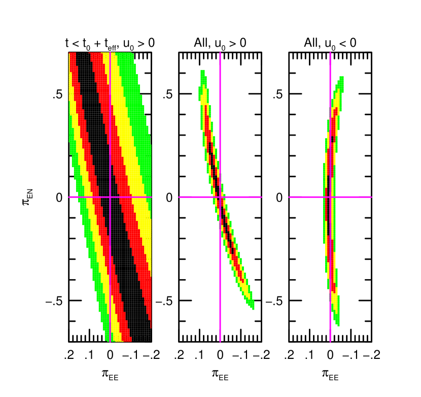
Figure 2: Ground-only ${\mbox{\boldmath$\pi$}}_{\rm E}$ contours for Event 1. In this, and all subsequent figures, the contour steps are set at $\Delta\chi^{2}=1,4,\ldots,n^{2}$.

The right two panels of Figure 2 show the final parallax measurement based on ground-only data, under the respective assumptions that $u_{0}>0$ and $u_{0}<0$, which is not known a priori. By themselves, the ground data clearly provide no information on the magnitude of $\pi_{\rm E}$, and hence on whether the lens is a BH or not. However, these data can potentially limit or rule out the possibility that the “alternative” ($\pi_{{\rm E},\rm large}$) solution (from the Refsdal 1966 analysis) is correct. Unless this solution lay on or near the one-dimensional structures shown in Figure 2, there could be no local minimum in the $\chi^{2}$ surface at the “alternative” solutions. Of course, one could determine whether a local minimum existed by conducting a grid search over the ${\mbox{\boldmath$\pi$}}_{\rm E}$ plane, but the point of the present exercise is to understand why we would expect, or not expect, such a minimum to exist. I will return to this issue in Section 4.3.1.

The reason for the one-dimensional structures in the two right-hand panels is well understood, at least in the limit of events with short effective timescales, $t_{\rm eff}\ll{\rm yr}/2\pi$, i.e., the same limit that underlies the parallax-satellite analyses of Refsdal (1966) and Gould (1994b). For short $t_{\rm eff}$ events, Earth’s (projected) acceleration toward the position of the Sun, S, is approximately constant, which induces an asymmetry in the light curve with respect to $t_{0}$, yielding a measurement of the component $\pi_{{\rm E},\parallel}$, whose direction is therefore

$$\Psi_{\parallel}=\tan^{-1}{-S_{E}(t_{0})\over-S_{N}(t_{0})}.$$ (13)

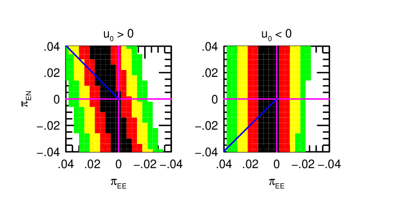
Figure 3: Zoom of the two right panels from Figure 2. The blue rays in this figure (and all subsequent figures) represent the directions inferred from the interferometric measurement.

The poorly measured component is then $\Psi_{\perp}=\Psi_{\parallel}+\pi/2=\tan^{-1}([-S_{N}(t_{0})]/S_{E}(t_{0}))$. See Figure 3 of Park et al. (2004) for sign conventions and for an example of a highly linear structure for an event with $t_{\rm eff}=2\,$day (keeping in mind that MOA-2003-BLG-37 peaked in the summer, whereas Event 1 peaks in the spring).

For Event 1, $(S_{N},S_{E})(t_{0})=(-0.075,+0.742)\,{\rm au}$. Hence, the expected direction of the linear structures in Figure 2 is $\Psi_{\perp}=5.8^{\circ}$, north through east.

While many such structures have been noted in the literature for short $t_{\rm eff}$ events, they have not, to the best of my knowledge, been systematically studied for moderately long events like Events 1 and 2, which have $t_{\rm eff}=21\,$day. From Figure 2, we see that the actual contours deviate from the short-$t_{\rm eff}$ prediction (and past short-$t_{\rm eff}$ experience) in two key ways. First, both sets of contours are curved, and with very similar curvature. Second, neither of the tangents at the best-fit values (i.e., centers of the structures) matches the $\Psi_{\perp}=5.8^{\circ}$ expectation. Instead, the $u_{0}>0$ tangent is $\sim 12^{\circ}$, while the $u_{0}<0$ tangent is $\sim 0^{\circ}$. Hence, they agree with the expectation in their average, but not individually.

Nevertheless, regardless of whether these 1-D structures exactly match theoretical expectations derived from the short-$t_{\rm eff}$ analysis, they greatly reduce the chances that the $\pi_{{\rm E},\rm large}$ solutions will survive the joint fit to the Earth and satellite data. In fact, as I will show in Section 4.3.1, the elimination of the $\pi_{{\rm E},\rm large}$ solutions is not really a matter of “chance” (as might appear from the present discussion). For now, I just note that for events that, like Events 1 and 2, lie toward the bulge and several degrees south of the ecliptic, $S_{N}$ retains a small negative value through most of the microlensing season, while $S_{E}$ moves from large positive values to large negative values. Thus $\Psi_{\perp}$ rotates counterclockwise over the course of the microlensing season from slightly east of north to slightly east of south.

The left panel of Figure 2 shows the parallax measurement derived from ground data at the time that I have specified for a “decision” regarding interferometric observations, i.e., at $t=t_{0}+t_{\rm eff}$. See also Figure 1. The first point is that the ground-only data do not contribute significant information toward making this decision compared to the information that will be available from the combined ground and satellite observations, which I will discuss in Section 4.2.3. Thus the panel may appear to be of little interest.

However, it is also of some value to consider how one would react to such a measurement if (as is true at present) there were no satellite, and hence no satellite data. First, one would conclude that $\pi_{{\rm E},\parallel}$ (the only measurable component) was consistent with zero, and so (given the long timescale, $t_{\rm E}=69\,$day) that this was a plausible BH candidate. From there, one would have been led to ask: under what conditions could an interferometric measurement yield a BH “detection”, and if so, then also a reliable mass measurement. One would consider various possible values of $\pi_{\rm E}$ that are consistent with the left panel, and simulate ground data from the rest of season. For example, for a trial $\pi_{\rm E}=0.0114$, such simulations would yield ${\mbox{\boldmath$\pi$}}_{\rm E}$ maps similar to the two right panels. As I will show just below, one would then immediately conclude that the parallax error (even with the direction of ${\mbox{\boldmath$\pi$}}_{\rm E}$ determined from interferometry), would be of order $\sigma(\pi_{\rm E})\sim 0.015$, so that a $3\,\sigma$ measurement would be possible only if $\pi_{\rm E}\gtrsim 0.05$ i.e., $\pi_{\rm rel}=\kappa M\pi_{\rm E}^{2}\gtrsim 0.2\,{\rm mas}$ (or $0.1\,{\rm mas}$), and $\mu_{\rm rel}=\kappa M\pi_{\rm E}/t_{\rm E}\gtrsim 22\,{\rm mas}\,{\rm yr}^{-1}$ (or $11\,{\rm mas}\,{\rm yr}^{-1}$) for an $M=10\,M_{\odot}$ (or $5\,M_{\odot}$) BH. While the first (higher-mass) scenario is quite unlikely, the lower-mass scenario is not implausible, and hence it is likely that the interferometric observations would have been undertaken.

We can judge the results from Figure 3, which provides zooms of the two right panels of Figure 2. The blue rays show the directions of ${\mbox{\boldmath$\pi$}}_{\rm E}$ implied by the interferometric measurement under the assumptions of $u_{0}>0$ and $u_{0}<0$, respectively. That is, because $\Phi_{\pi}=\tan^{-1}(\pi_{{\rm E},E}/\pi_{{\rm E},N})=44.6^{\circ}$, and $\phi=\cot^{-1}(\delta t/t_{\rm eff})\rightarrow 45^{\circ}$, while $u_{0}>0$, the major image will lie at $\psi=\Phi_{\pi}+\phi+\pi=269.6^{\circ}$ relative to the $y$-axis, i.e., approximately due west. Then, of course, if one interprets this measurement under the (correct) assumption that $u_{0}>0$, one will recover $\Phi_{\pi}=\Psi-\phi-\pi=44.6^{\circ}$. However, under the assumption that $u_{0}<0$, one will infer $\Phi_{\pi}=\Psi+\phi-\pi=134.6^{\circ}$. More generally, the $u_{0}<0$ solution will always lie $2\phi$ counterclockwise from the $u_{0}>0$ solution and, in particular, $90^{\circ}$ counterclockwise if the observation is at $t=t_{0}+t_{\rm eff}$. See Equations (6) and (7).

The net result is that one would conclude that $\pi_{\rm E}<0.05$ at the $3\,\sigma$ level, but with no lower limit (even at $1\,\sigma$), and one would simultaneously obtain a relatively precise measurement of $\theta_{\rm E}=1.11\,{\rm mas}$. Together these would imply $M=\theta_{\rm E}/\kappa\pi_{\rm E}>2.7\,M_{\odot}$ and $\pi_{\rm rel}=\theta_{\rm E}\pi_{\rm E}<57\,\mu{\rm as}$. This would be a very secure detection of either a BH or neutron star (NS), with the BH strongly favored, partly by the fact that such massive NSs are expected to be rare, and partly by the fact that such low values of the measured mass are permitted only at $3\,\sigma$. However, there would be no information at all on the mass of the BH, and there would be no clear indication of whether it was in the disk or the bulge.

4.2.2 Ground+Satellite Analysis

Figure 4 shows the results of simultaneously fitting the ground and satellite data under three different assumptions about the flux constraint, i.e., that the ratio of source fluxes as seen from the ground and the satellite can be constrained to 2.5% (lower panels), 0.25% (middle panels), and 0.025% (upper panels). The first is essentially no constraint because the source fluxes from the fit can be determined to better than this precision. I consider the second to be realistic, provided that the wavelength dependence of the satellite and ground systems are similar. I do not consider the third to be realistic, but it represents a theoretical limit on what can be achieved by externally constraining the flux ratio. The $\chi^{2}$ contours are shown relative to the minimum in each panel. The $\chi^{2}$ difference between the two panels in the same row are indicated within the $u_{0}<0$ panels.

The first point to note is that the improvements from the lower to middle panels is substantially larger than than that from the middle to the upper panels. Similarly, the improvements in $\Delta\chi^{2}$ also show a much larger jump. This implies that the “realistic” flux constraint is both useful in constraining ${\mbox{\boldmath$\pi$}}_{\rm E}$ and cannot be much improved upon, even by exceptional efforts. Henceforth, I will therefore focus on the middle panels.

Second, for both $u_{0}>0$ and $u_{0}<0$, the contours are elongated at a substantial angle relative to the cardinal axes. This is somewhat surprising in light of the discussion in Section 3.2, wherein I argued that the errors in the $\Delta t_{0}$ and $\Delta t_{\rm eff}$ should be uncorrelated, which would imply that any departure from isotropy in the error ellipses should take the form of elongation either parallel or perpendicular to ${\bf D}_{\perp}$. While it is true that ${\bf D}_{\perp}$ changes substantially over the course of the event, its direction is remains roughly fixed along the east-west axis. See the upper panel in Figure 1. In particular, Gould (1995) had argued that the errors in $\Delta u_{0}$ should be larger than those in $\Delta t_{0}/t_{\rm E}$, which would lead to a north-south elongation of the error ellipses. The origin of this unexpected behavior can be seen in Figure 1, which shows that the satellite observations do not begin until a few days before peak, which invalidates the underlying assumption of approximately symmetric coverage about $t_{0}$ that was the basis of the statistical independence of $t_{0}$ and $u_{0}$ for each observatory, and thus of $\Delta t_{0}$ and $\Delta u_{0}$. Instead, this strong asymmetry in coverage leads to a strong correlation between $t_{0,\rm sat}$ and $u_{0,\rm sat}$. Indeed, such correlations can become even more pronounced for the case that the satellite observations begin long after $t_{0}$, in which case they can lead to large arcs on the ${\mbox{\boldmath$\pi$}}_{\rm E}$ plane (Gould, 2019). See Zang et al. (2020) for a dramatic example of such an arc, which was nevertheless resolved by VLTI interferometry.

Third, in this case the ambiguity between the two $\pi_{{\rm E},\rm small}$ solutions is only marginally resolved because the directional constraint (blue ray) for the “wrong” solution (right-middle panel) passes close enough to the $\chi^{2}$ minimum that it must be considered, while the difference between the minima is only $\Delta\chi^{2}=7$. Happily, and as anticipated, the magnitude $\pi_{\rm E}=|{\mbox{\boldmath$\pi$}}_{\rm E}|$ is essentially the same for both solutions, so this ambiguity does not strongly affect the mass and distance estimates, but it does impact the directional information. Hence, this event is one that would profit from a second interferometric observation, which would definitively resolve this ambiguity. In Section 4.2.3, I will discuss whether the decision to undertake such a second observation could be made sufficiently quickly. For now I note that even for this event, which is near the margin of a reliable BH mass measurement (and was chosen as an example for that reason), the chance of even marginal survival of the alternate $\pi_{{\rm E},\rm small}$ solution is only about 15%. To understand this, the first point to note is that each event has equal prior probability of having $u_{0}>0$ or $u_{0}<0$. If I had simulated the latter case (with all other parameters being the same), then the two sets of contours in the middle row would have been approximately flipped about the $x$-axis, but slightly shifted so that the $\chi^{2}$ minimum in the right panel exactly coincided with the actual parallax, while the minimum of the left panel would be slightly displaced from its flipped position. The blue ray in the right panel would likewise be flipped, so that it would pass exactly through the $\chi^{2}$ minimum. However, the blue ray in the left panel would not pass through its contours (now centered in the lower-left quadrant) because it would pass through the (essentially empty) upper-right quadrant. That is, the directional constraint for $u_{0}>0$ lies $90^{\circ}$ clockwise from the $u_{0}<0$ constraint (for interferometric observations at $t=t_{0}+t_{\rm eff}$). More generally, one should consider an ensemble of random directions for $\Phi_{\pi}$ and both signs of $u_{0}$. At the small values of $\pi_{\rm E}$ probed by these diagrams, the contours will retain their size, shape, and orientation as the “true solution” is changed. Hence, the probability of a marginally resolved ambiguity is just the average angle subtended by the $2\,\sigma$ contours as they are transported around the $\pi_{\rm E}=0.0114$ circle (and averaged over both signs of $u_{0}$). Note, then, that the values of $\Phi_{\pi}$ with the smallest chance for a surviving ambiguity (i.e., those for which the the long axis of the contours point toward the origin), are also the ones with the greatest errors in the $\pi_{\rm E}$ measurement. The actual case shown in Figure 4 is the opposite: the error ellipse is transverse to directional constraint, which minimizes the $\pi_{\rm E}$ error, but maximizes the chance of survival of the ambiguity.

Finally, I note that a wider grid search rules out any additional (i.e., $\pi_{{\rm E},\rm large}$) solutions. I discuss the underlying reasons for this in Section 4.3.1.

4.2.3 Interferometric Decisions

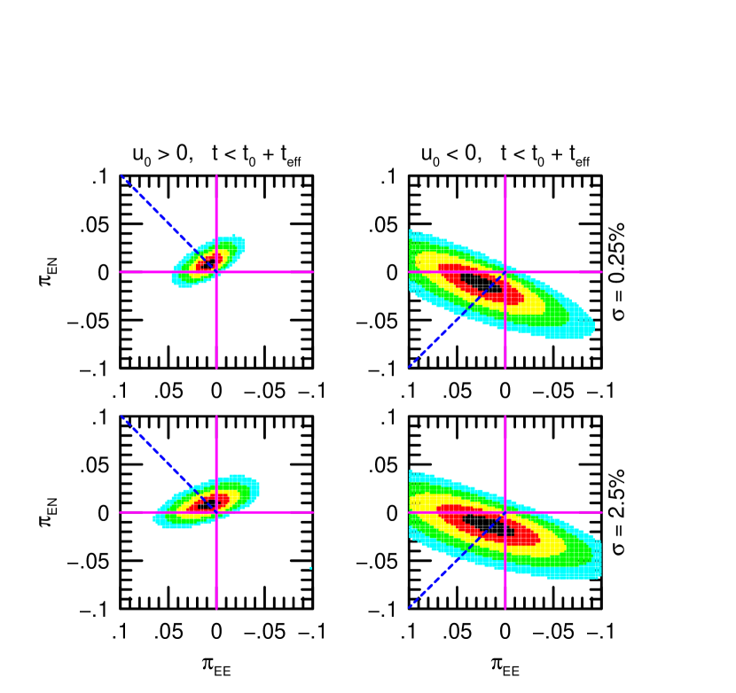
Figure 5: ${\mbox{\boldmath$\pi$}}_{\rm E}$ contours from combined ground and satellite data that have been collected for Event 1 at the time of the interferometric decision, i.e., $t=t_{0}+t_{\rm eff}$. The blue rays are shown as dashed because the interferometric result is not known when the decision is made to conduct this measurement, but is known when a second decision must be made on whether to obtain an additional interferometric measurement.

Figure 5 shows the ${\mbox{\boldmath$\pi$}}_{\rm E}$ contours at the time of the decisions about interferometric observations, i.e., $t=t_{0}+t_{\rm eff}$, for both the weak ($\sigma=2.5\%$) and “realistic” ($\sigma=0.25\%$) external flux constraints. Note that the scale is 5 times larger than the corresponding panels in Figure 4. Also note that the blue rays that represent the interferometric direction measurement are shown as dashed lines to indicate the dual role of these diagrams: Based on the contours alone (no blue rays) one must decide whether the event is a sufficiently good candidate to make the interferometric measurement. Then, after the measurement (so, with blue ray), one must decide whether it will be necessary to make an additional measurement to break the directional degeneracy.

The first point is that including the “realistic” flux constraint does not qualitatively improve the decision process. In any case, I subsequently refer to the “realistic” case, i.e., the upper panels. Based on these, and at the $2\,\sigma$ level, $0.01\lesssim\pi_{\rm E}\lesssim 0.03$ and $0.01\lesssim\pi_{\rm E}\lesssim 0.07$ for $u_{0}>0$ and $u_{0}<0$, respectively. Thus, using Equation (8) one finds that the $u_{0}<0$ solution is consistent with an ordinary $M=1\,M_{\odot}$ star with proper motion $\mu_{\rm rel}=3\,{\rm mas}\,{\rm yr}^{-1}$. Nevertheless, if true, the chance that the much more tightly constrained $u_{0}>0$ contours would lie so close to the origin is only about 25%. There might be additional information from the FWHM$\sim 0.4^{\prime\prime}$ satellite images that ruled out main-sequence lenses down to, say, $0.8\,M_{\odot}$, which could further inform the decision. In the end, there would nevertheless be some risk that this was an ordinary star, which could be mitigated by waiting to, e.g. $t=t_{0}+2\,t_{\rm eff}$, when the source was fainter by 0.5 magnitudes. The final decision would have to take account of the feasibility of such future observations (based on brightness, reference stars etc.), the time pressure on the instrument, and the general level of risk that could be supported.

On the assumption that measurement was made, the result (intersection of the blue rays with the contours), would imply that, at $2\,\sigma$, $0.01\lesssim\pi_{\rm E}\lesssim 0.02$ and $0.01\lesssim\pi_{\rm E}\lesssim 0.04$ for the two cases. Moreover, $\theta_{\rm E}=1.11\,{\rm mas}$ would now be measured, implying $M=\theta_{\rm E}/\kappa\pi_{\rm E}\gtrsim 3.4\,M_{\odot}$, i.e., a BH. The fact that the blue rays come close to both minima would indicate that it was unlikely that the ambiguity would be decisively resolved by the full season of observations and hence that an additional interferometric measurement was warranted. For example, by waiting just 3 days, the positional angle of the major image relative to the minor image would rotate by $\sim 4^{\circ}$, either clockwise for $u_{0}>0$ or counterclockwise for $u_{0}<0$.

Finally, I note that a comparison of the upper left panel of Figure 5 with the left panel of Figure 2 shows that the ground-only data plays almost no role in constraining the combined-data contours. For example, the black contours in Figure 2 intersect the $x$-axis over the range $+0.05>\pi_{{\rm E},E}>-0.04$, which is very large on the scale of the contours in Figure 5.

4.3 Event 2

When analyzing Event 2, I mainly focus on understanding the differences in results compared to Event 1. These are quite dramatic given that the only differences in event parameters are that $t_{0}$ is four months later and the sign of $\pi_{{\rm E},E}$ is reversed.

4.3.1 Ground-Only Analysis

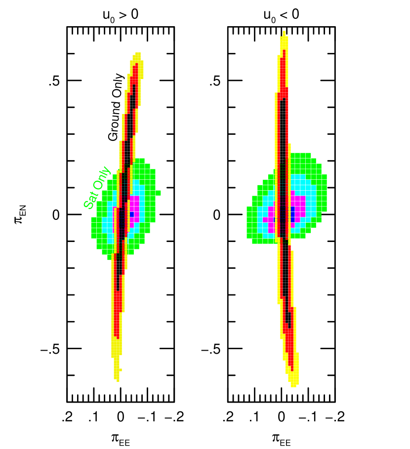
Figure 6: ${\mbox{\boldmath$\pi$}}_{\rm E}$ contours for Event 2, based on ground-only (black, red, yellow) and satellite-only (blue, magenta, cyan, green) data.

The nearly-linear (black, red, yellow) contours in Figure 6 show the constraints on ${\mbox{\boldmath$\pi$}}_{\rm E}$ from ground-only data for Event 2. These can be compared to the analogous contours for Event 1 that are displayed in Figure 2. The most striking difference is that the constraints on $\pi_{{\rm E},\parallel}$ (width of the contours) are weaker by a factor $\sim 2$. At least a partial explanation for this difference is that $t_{0}$ for Event 2 is closer to the end of the ground microlensing season than $t_{0}$ for Event 1 is to the beginning. Therefore, the asymmetry in the data with respect to $t_{0}$, from which the value of $\pi_{{\rm E},\parallel}$ is extracted, is less well traced by the data for Event 2.

A seemingly minor technical point is that the ground-only contours in the $u_{0}>0$ panel of Figure 6 appear to be rotated clockwise by about $16^{\circ}$. Strictly speaking, as explained in Section 4.2.1, they have been rotated counterclockwise by $164^{\circ}$. Applying the analysis given there, I find that at $t_{0}$ for Event 2, $(S_{N},S_{E})(t_{0})=(-0.021,-0.952)\,{\rm au}$. Hence, based on the short-$t_{\rm E}$ formalism, we expect that the long axis of the contours should be nearly straight and point $179^{\circ}$ (north through east). As in Figure 2, both sets of ground-only contours are curved, and as in that Figure, the tangents to the arcs at the best fit are not the same, being roughly $-4^{\circ}$ and $+2^{\circ}$ for $u_{0}>0$ and $u_{0},0$, respectively. That is, their average is $-1^{\circ}$, which (after a $180^{\circ}$ rotation) agrees with the short-$t_{\rm E}$-framework prediction, as was also true for Event 1.

The reason that it is important to distinguish between a $16^{\circ}$ clockwise rotation and a $164^{\circ}$ counterclockwise rotation is that this rotation helps to understand how the $\pi_{{\rm E},\rm large}$ solutions are automatically excluded by the satellite data in most cases.

As discussed in Section 4.1, the satellite trails Earth’s orbit by about 82 days. Thus, as seen from the satellite, the Sun’s position at $t_{0}$ is the same as it would be from Earth, but 82 days earlier, i.e., about 10 June, at which point $(S_{N},S_{E})(t_{0})=(-0.099,+0.140)\,{\rm au}$. In fact, a precise calculation based on the actual Spitzer orbit that is being used in these calculations gives $(S_{N},S_{E})_{\rm sat}(t_{0,\rm ground})=(-0.082,+0.153)\,{\rm au}$. However, for purposes of understanding the underlying issues, it is easier to think about the more familiar Earth orbit near 10 June than the more precise satellite orbit near 1 September. At this time, the event is nearly in opposition, which actually occurs on 18 June, when $S_{E}=0$. During the $2|S_{N}|{\rm yr}/2\pi=12\,$days from before to after opposition, $\Psi_{\parallel}$ rotates by $90^{\circ}$. Hence during these times, the constant-acceleration formalism is not even remotely applicable for Event 2, which has $t_{\rm eff}=21\,$days. Therefore, we do not expect the ${\mbox{\boldmath$\pi$}}_{\rm E}$ contours that are derived from satellite-only data to be long, linear structures. Nevertheless, we do expect that they will be very different from the ground-only contours. Figure 6, which displays the satellite-only contours in (blue, magenta, cyan, green) confirms this expectation. In particular, there is no overlap between the two sets of contours for $\pi_{{\rm E},\rm large}\simeq 2u_{0}({\rm au}/D_{\perp})\sim 0.6$ at any orientation $\Phi_{\pi}$.

While the particular contours shown in Figure 6 are specific to Event 2, it will always be the case that if the satellite trails (or leads) Earth by enough to make a reliable measurement of $\Delta t_{0}$ and $\Delta u_{0}(+,+)$ for a BH lens, then the ground-only and satellite-only contours will be substantially different, particularly at large $\pi_{\rm E}$. Hence, except for relatively high-magnification events (for which $\pi_{{\rm E},\rm large}$ is not very big, and for which it may be the correct solution, even for BH events), the combination of ground-only and satellite-only fits will, by themselves almost always exclude the $\pi_{{\rm E},\rm large}$ solutions.

Stepping back, once there are dense satellite data that well cover the peak (which applies fully to Event 2, but only partially to Event 1), there are actually three, quasi-independent, constraints on ${\mbox{\boldmath$\pi$}}_{\rm E}$: first on $(\Delta t_{0},\Delta u_{0})$ from comparison of the Paczyński (1986) parameters of the ground-only and satellite-only fits; second from the distortions induced by the accelerated motion of Earth on the ground-based light curve; and third from the distortions induced on the satellite-based light curve due to its acceleration.

For BH events of modest peak magnification, the first of these three leaves a four-fold degeneracy, but provides nearly all the information about each of the four local minimum, while the combination of the latter two provides very little information about the two $\pi_{{\rm E},\rm small}$ solutions, but decisively excludes the two $\pi_{{\rm E},\rm large}$ solutions.

4.3.2 Ground+Satellite Analysis

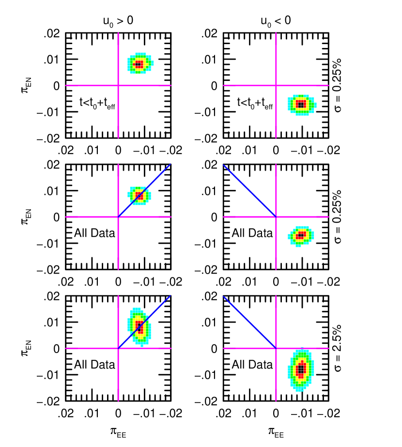
Figure 7: The lower four panels show the ${\mbox{\boldmath$\pi$}}_{\rm E}$ contours from combining all of the ground and satellite data for Event 2. “Realistic” and very weak flux constraints are applied for the middle and lower panels, respectively. These can be compared directly to the lower four panels of Figure 4. The two upper panels show the ${\mbox{\boldmath$\pi$}}_{\rm E}$ contours as of the time of the interferometric decision, i.e., $t=t_{0}+t_{\rm eff}$.

The lower four panels of Figure 7 show the ${\mbox{\boldmath$\pi$}}_{\rm E}$ contours for Event 2 for the cases of both the “realistic” and weak flux constraints. These can be directly compared to the lower four panels of Figure 4. The differences are striking. First, the error ellipses are dramatically smaller in all four cases. Second, the interferometric measurement of the direction (blue rays) decisively rules out the $u_{0}<0$ solution for Event 2.

The reasons for the smaller error ellipses can be understood directly from Figure 1. From the top panel, we see that $D_{\perp}(t_{0})\sim 1\,{\rm au}$ for Event 2, whereas it is an order of magnitude smaller for Event 1. The result is that the Earth (blue) and satellite (magenta) peaks are clearly separable by eye in both time and amplitude for Event 2, while they appear indistinguishable for Event 1. (For Event 1, most of the information about $\Delta t_{0}$ and $\Delta u_{0}$ comes from the falling part of the light curve, over which $D_{\perp}$ is rapidly growing. However, the resulting differences in the two light curves do not yield features that are discernible by eye.)

The fact that the interferometric measurement rules out the alternate $\pi_{{\rm E},\rm small}$ solution is a matter of chance in two senses. First, if the $u_{0}<0$ solution had been correct, then the interferometric measurement would (of course) have resulted in a blue ray that passed directly through the correct solution (which would be in the right panels). However, in this case, the blue ray in the left panels would lie $90^{\circ}$ counterclockwise from this orientation, which would be approximately its current location, i.e., passing directly through the (wrong) $u_{0}>0$ solution. Hence, this aspect is a 50-50 chance.

The second aspect of chance is much more one-sided. The two blue rays are displaced by $90^{\circ}$ because the interferometric observations occur at $t_{0}+t_{\rm eff}$. At other times, the displacement would differ by $2\phi$ where $\cot\phi=\delta t/t_{\rm eff}$, as described by Equation (6). On the other hand, the two solutions are separated by $\sim 2\tan^{-1}|\pi_{{\rm E},E}/\pi_{{\rm E},N}|$ (where I have assumed that ${\bf D}_{\perp}$ is approximately west). In the examples that I have given, with $|\pi_{{\rm E},N}|\simeq|\pi_{{\rm E},E}|$, this just happens to be about $90^{\circ}$, but for other values it would be different. For cases like Event 2, with small error ellipses, it will be rare that these two angles agree closely enough to leave an ambiguity in the $\pi_{{\rm E},\rm small}$ solutions.

4.3.3 Interferometric Decisions

The upper row of Figure 7 shows the ${\mbox{\boldmath$\pi$}}_{\rm E}$ contours at the time of the interferometric decision, $t=t_{0}+t_{\rm eff}$, assuming the “realistic” flux constraint. Both sets of contours are well-localized, with $\pi_{\rm E}$ near its actual value of 0.0114. Hence, the inferred proper motion for a putative $1\,M_{\odot}$ lens would be $\mu_{\rm rel}=\kappa M_{\odot}\pi_{\rm E}/t_{\rm E}\sim 0.5\,{\rm mas}\,{\rm yr}^{-1}$, i.e., well beyond any plausible threshold for a positive decision. Comparing these contours to those in the middle row of Figure 5 shows vastly higher precision for Event 2 compared to Event 1. As with the full-dataset comparison that was discussed in Section 4.3.2, this is due partly to larger $D_{\perp}$ near $t_{0}$ and partly to the longer data stream from the satellite.

5 Discussion

5.1 Extreme Applications, Challenges, and Orbits

In Sections 1–3, I have argued for the feasibility of industrial-scale BH mass measurements and have illustrated and further investigated this with two example events in Section 4. By choosing a relatively large value of the Earth-satellite separation, $D_{\rm sat}\sim 1.3\,{\rm au}$, I was able to illustrate some of the most powerful applications as well as the most severe challenges of the method.

Regarding the first, the $3\,\sigma$ (yellow) error contours in the middle-left panel of Figure 7 are $\sim 5$ times smaller than the value of $\pi_{\rm E}$, which means that a three-times smaller parallax could be measured with $\sim 20\%$ precision. For a typical bulge $\pi_{\rm rel}\sim 15\,\mu{\rm as}$, this would correspond to an $M=128\,M_{\odot}$ BH. Thus, if there were a bulge population of very massive BHs, e.g., from an early era of massive star formation, they could be reliably detected and accurately measured. This sensitivity is made possible in part by the large $D_{\rm sat}\sim 1.3\,{\rm au}$, which allowed $D_{\perp}\sim 1\,{\rm au}$ over the peak of Event 2 (see Figure 1).

However, the same wide separation also creates challenges. Given the $45^{\circ}$ Sun-exclusion angle, observations could be made only starting on 23 April. Engineering a smaller Sun-exclusion angle would be difficult, and (unless it were at least $10^{\circ}$ smaller), there would be hardly any benefit because $D_{\perp}$ would be very small at these times. Measurements of ${\mbox{\boldmath$\pi$}}_{\rm E}$ could be made for events with $t_{0}$ before this date, but they would have substantially larger $t_{0}$–$u_{0}$ correlations than Event 1, and therefore substantially larger errors, which are already dramatically larger than for Event 2.

If $D_{\rm sat}$ were reduced, say to $0.6\,{\rm au}$, both aspects, i.e., the power and the challenges would be reduced. For events peaking late in the microlensing season, like Event 2, the errors would be increased by a factor $\sim 2$ because $D_{\perp}$ would be roughly half as big as in Event 2 as it was simulated in this paper. On the other hand, the error bars would be substantially improved for Event 1. First, at $t_{0}$ (1 May), the projected satellite separation would be $D_{\perp}\sim 0.5\,{\rm au}$. i.e., about half of the value for Event 2 in Figure 1. Second, satellite observations could commence $\sim 35\,$days earlier, i.e., about 19 March, yielding much better coverage of the rising part of the satellite light curve. Moreover, events could be observed that peaked up to a month earlier than those that could be observed with $D_{\rm sat}\sim 1.3\,{\rm au}$.

To fully assess all possible orbits would be well beyond the scope of the present work. I only raise this question to make clear that there is an issue here. One could also consider a variable orbit. For example, the satellite could start with a semi-major axis $a=1.03\,{\rm au}$, so that it $dD_{\rm sat}/dt\sim 0.3\,{\rm au}$/yr and thus quickly achieve $D_{\rm sat}\sim 0.6\,{\rm au}$ after 2 years. Then the orbit could changed to $a=1.01\,{\rm au}$, thus reducing the drift to $dD_{\rm sat}/dt\sim 0.1\,{\rm au}$/yr. This would make the satellite more sensitive to BHs overall early in its mission, but more sensitive to extreme BHs later on.

5.2 Comparison to Gould & Yee (2014)

Gould & Yee (2014) proposed another approach to industrial-scale BH mass measurements, which was further examined by Gould et al. (2023). Here, I briefly describe this technique, which rests on a technology that is still under development, and I compare its promise and challenges to those of the approach presented here.

The Gould & Yee (2014) approach is to exploit the data stream arising from a wide-field space-based microlensing planet survey, such as Roman (formerly WFIRST), Euclid, or CSST. I will specifically consider Roman because its microlensing-survey characteristics are approximately known. The basic idea is to combine measurements of $\pi_{{\rm E},\parallel}$ (derived from photometric measurements of the source) and ${\mbox{\boldmath$\theta$}}_{\rm E}\equiv{\mbox{\boldmath$\mu$}}_{\rm rel}t_{\rm E}$ (derived from astrometric measurements of the source), to yield $\pi_{\rm E}$ and $\theta_{\rm E}$, and so $M=\theta_{\rm E}/\kappa\pi_{\rm E}$ and $\pi_{\rm rel}=\theta_{\rm E}\pi_{\rm E}$. The Roman microlensing survey is expected to monitor an area of $\Omega_{Roman}\sim 2.5\,{\rm deg}^{2}$ at a cadence of $\Gamma\sim 4\,{\rm hr}^{-1}$ for 6 different 72-day campaigns, each centered approximately on an equinox. Roman has a 2.4m mirror, and the project will be carried out using a broad $H$-band filter.

Being centered on the equinoxes, the 72-day campaigns are well suited to measuring 1-D parallaxes. Moreover, it is plausible to expect photometric errors that are near the photon limit and uncorrelated in time. The key issue, as already recognized by Gould & Yee (2014), is whether the astrometric measurements will be similarly well-behaved. If they are, then it is straightforward to calculate how well the magnitude and direction of ${\mbox{\boldmath$\theta$}}_{\rm E}$ can be measured from the “astrometric microlensing” technique that I described in Section 1.

Gould et al. (2023) carried out simulations of this approach for a limited number of cases. They characterized the conditions needed to measure BH masses of bulge BHs with typical microlens parallaxes $\pi_{\rm E}\sim 0.014$ as $u_{0}\lesssim 0.4$, $\sigma_{\rm phot}<0.01$, and $0<(t_{0}-t_{\rm equinox}){\rm sgn}_{\rm equinox}<36\,$day. Here, $t_{\rm equinox}$ is the time of equinox (about 21 March or 21 September) and ${\rm sgn}_{\rm equinox}$ is $+1$ for the vernal equinox and $-1$ for the autumnal equinox. They estimated that their photometric-precision limit obtains for sources with $H_{\rm Vega}=20.4$ or $M_{H}=5.3$ (M0 dwarfs). As Gould et al. (2023) themselves emphasized, their limited simulations are no substitute for a systematic investigation of the Gould & Yee (2014) approach. Nevertheless, I will use them here as a rough guide because they constitute the only study that has been carried out to date.

To compare to the approach here, I estimate (based on Section 4) a limit of $I=19.8$ (or $M_{I}=3.25$, assuming typical $A_{I}=2.0$), $u_{0}<0.4$, and a range of $t_{0}$ covering 150 days per season. I estimate an “effective area coverage” of $\Omega_{\rm eff}=25\,{\rm deg^{2}}$. That is, even though the ground survey covers $\sim 100\,{\rm deg^{2}}$, the event rate in the outlying fields is substantially lower than in the Roman fields. There are then three factors that must be combined to compare the two approaches: area, time interval, and luminosity function. For the first, $\Omega_{\rm eff}/\Omega_{Roman}=10$. For the time interval, Roman has $6\times 36=216\,$days of sensitivity, whereas the approach presented here would have $5\times 150=750\,$days for a 5-yr mission, which yields a ratio of $\sim 3.5$. To evaluate the ratio of allowed regions of the luminosity function, I first convert the Roman limit to $M_{I}=7.0$, and then apply the Holtzman et al. (1998) luminosity function to obtain a ratio of $1/12.5$. Combining the three factors, I obtain a net advantage of a factor $10\times 3.5/12.5\sim 2.8$ in favor of the method presented here. I must emphasize that my calculation is both crude and only applies to one type of BH (namely bulge BHs). So the main conclusion is that in terms of numbers of BH mass measurements under ideal conditions, the two approaches are comparable.

The main advantage of the Gould & Yee (2014) approach is that no special effort is required to obtain the data: assuming a successful launch and successful operations, the data stream will “just appear” in a publicly available archive.

The main disadvantage is that there is really no way to determine in advance whether it will actually work, i.e., whether the astrometric errors from many thousands of measurements can be treated as independent and can therefore be combined according to naive statistics (as assumed by Gould et al. 2023 in the above-cited calculations). At the $\sigma_{\rm phot}=0.01$ threshold, a single measurement has an error of $\sigma_{\rm ast,1}=1\,{\rm mas}$. We can conceptually bin the data in one-week bins, which are satisfactory for tracing the astrometric evolution. Then, assuming uncorrelated errors, each has an error of $\sigma_{\rm ast,week}=40\,\mu{\rm as}$, or about $4\times 10^{-4}$ pixels. Hence, to achieve the overall precision calculated by Gould et al. (2023), there cannot be unmodeled systematic trends in the data (due to either instrumental or astrophysical causes) at this level. Gould & Yee (2014) give an overview of the Rumsfeld triad of known-known, known-unknown, and unknown-unknown systematic errors. I refrain from rehearsing these here. I will just note that the difficulty of interpreting the Hubble Space Telescope (HST) astrometry for the case of OGLE-2011-BLG-0462 (Sahu et al., 2022; Lam et al., 2022; Mróz et al., 2022) provides a sobering note of caution. First, the resolution is 2 times better for HST than Roman. Second, the HST sampling of the PSF is somewhat better. Third, the astrometric precision required was almost an order of magnitude less severe than what will be required for the Gould & Yee (2014) approach. Yet, Sahu et al. (2022) and Lam et al. (2022) obtained substantially different estimates of the direction of ${\mbox{\boldmath$\pi$}}_{\rm E}$ (or ${\mbox{\boldmath$\mu$}}_{\rm rel}$), which was only resolved (in favor of the first) by additional work by Mróz et al. (2022).

Happily, as pointed out by Gould & Yee (2014), there are robust methods for determining whether or not the final results have been corrupted by systematic errors, regardless of whether or not these systematic errors can be identified. However, these tests can only be carried out after the fact.

My conclusion is that both approaches should be vigorously pursued.

Figure 4: ${\mbox{\boldmath$\pi$}}_{\rm E}$ contours from combined ground and satellite data for Event 1 for three different values of the constraint on the ratio of source fluxes as seen from the ground and the satellite, which are indicated to the right. Also shown is the $\Delta\chi^{2}$ difference between the minima of the $u_{0}<0$ solution relative to the $u_{0}>0$ solution.

References

- Calchi Novati et al. (2015) Calchi Novati, S., Gould, A., Udalski, A., et al. 2015, ApJ, 804, 20
- Cassan et al. (2021) Cassan, A., Ranc, C., Abel, O., et al., 2021, Nature Astronomy, 6, 121
- Delplancke et al. (2001) Delplancke, F., Górski, K.M., & Richichi, A. 2001, A&A, 375, 701
- Dong et al. (2007) Dong, S., Udalski, A., Gould, A., et al. 2007, ApJ, 664, 862
- Dong et al. (2019) Dong, S., Mérand, A., Delplancke-Strobale, F. 2019, ApJ, 871, 70
- Einstein (1936) Einstein, A. 1936, Science, 84, 506
- Gould (1992) Gould, A. 1992, ApJ, 392, 442
- Gould (1994a) Gould, A. 1994a, ApJ, 421, L71
- Gould (1994b) Gould, A. 1994b, ApJ, 421, L75
- Gould (1995) Gould, A. 1995, ApJ, 441, L21
- Gould (1999) Gould, A. 1999, ApJ, 514, 869
- Gould (2000) Gould, A. 2000, ApJ, 542, 785
- Gould (2004) Gould, A. 2004, ApJ, 606, 319
- Gould (2019) Gould, A. 2019, JKAS, 52, 121
- Gould (2022) Gould, A. 2022, arXiv:2209.12501
- Gould et al. (1994) Gould, A., Miralda-Escudé, J. & Bahcall, J.N. 1994, ApJ, 423, L105
- Gould et al. (2009) Gould, A., Udalski, A., Monard, B. et al. 2009, ApJ, 698, L147
- Gould et al. (2010) Gould, A., Dong, S., Bennett, D.P. et al. 2010, ApJ, 710, 1800
- Gould & Horne (2013) Gould, A. & Horne, K. 2013, ApJ, 779, L28
- Gould & Yee (2014) Gould, A. & Yee, Y.C. 2014, ApJ, 784, 64
- Gould et al. (2020) Gould, A., Ryu, Y.-H., Calchi Novati, S., et al. 2020, JKAS, 53, 9
- Gould et al. (2022) Gould, A., Jung, Y.K., Hwang, K.-H. et. al., 2022, JKAS, 55, 173
- Gould et al. (2023) Gould, Ryu, Y.-H., Yee, J.C., et. al., 2023, AJ, 166, 100
- GRAVITY Collaboration et al. (2017) GRAVITY Collaboration, Abuter, R. Accardo, M., et al. 2017, A&A, 602, A94
- GRAVITY Wide Collaboration et al. (2022) GRAVITY Wide Collaboration, Abuter, R. Allouche, F., et al. 2022, A&A, 665, A75
- GRAVITY+ Collaboration et al. (2022) GRAVITY+ Collaboration, Abuter, R. Alarcon, P., et al. 2022, The Messenger, 189, 17
- Han et al. (2018) Han, C., Jung, Y.K., Shvartzvald, Y., et al. 2018, ApJ, 865, 14
- Hog et al. (1995) Hog, E., Novikov, I.D., & Polanarev, A.G. 1995, A&A, 294, 287
- Holtzman et al. (1998) Holtzman, J.A., Watson, A.M., Baum, W.A., et al. 1998, AJ, 115, 1946
- Kim et al. (2018) Kim, D.-J., Kim, H.-W., Hwang, K.-H., et al., 2018, AJ, 155, 76
- Lam et al. (2022) Lam, C.Y., Lu, J.R., Udalski, A., et al., 2022, ApJ, 933, L23
- Mao & Paczyński (1966) Mao, S. & Paczyński, B. 1996, ApJ, 473, 57
- Miyamoto & Yoshii (1995) Miyamoto, M. & Yoshii, Y. 1995, AJ, 110, 1427
- Mróz et al. (2022) Mróz, P, Udalski, A., & Gould, A., 2022, ApJ, 937, L24
- Nemiroff & Wickramasinghe (1994) Nemiroff, R.J., & Wickramasinghe, W.A.D.T. 1994, ApJ, 424, L21
- Paczyński (1986) Paczyński, B. 1986, ApJ, 304, 1
- Park et al. (2004) Park, B.-G., DePoy, D.L.., Gaudi, B.S., et al. 2004, ApJ, 609, 166
- Refsdal (1966) Refsdal, S. 1966, MNRAS, 134, 315
- Sahu et al. (2022) Sahu, K.C., Anderson, J., Casertano, S., st al. 2022, ApJ, 933, 83
- Shan et al. (2021) Shan, Y., Yee, J.C., Bailey, V. et al. 20121 ApJ, 908, 240
- Walker (1995) Walker, M.A. 1995, ApJ, 453, 37
- Witt & Mao (1994) Witt, H.J., & Mao, S. 1994, ApJ, 429, 66
- Yee et al. (2012) Yee, J.C., Shvartzvald, Y., Gal-Yam, A. et al. 2012, ApJ, 755, 102
- Yee et al. (2015) Yee, J.C., Gould, A., Beichman, C., 2015, ApJ, 810, 155
- Zang et al. (2020) Zang, W., Dong, S., Gould, A., et al. 2020, ApJ, 897, 180