Automaton Distillation: Neuro-Symbolic Transfer Learning for Deep Reinforcement Learning

Abstract

Reinforcement learning (RL) is a powerful tool for finding optimal policies in sequential decision processes. However, deep RL methods suffer from two weaknesses: collecting the amount of agent experience required for practical RL problems is prohibitively expensive, and the learned policies exhibit poor generalization on tasks outside of the training distribution. To mitigate these issues, we introduce automaton distillation, a form of neuro-symbolic transfer learning in which Q-value estimates from a teacher are distilled into a low-dimensional representation in the form of an automaton. We then propose two methods for generating Q-value estimates: static transfer, which reasons over an abstract Markov Decision Process constructed based on prior knowledge, and dynamic transfer, where symbolic information is extracted from a teacher Deep Q-Network (DQN). The resulting Q-value estimates from either method are used to bootstrap learning in the target environment via a modified DQN loss function. We list several failure modes of existing automaton-based transfer methods and demonstrate that both static and dynamic automaton distillation decrease the time required to find optimal policies for various decision tasks.

Introduction

Sequential decision tasks, in which an agent seeks to learn a policy to maximize long-term reward through trial and error, are often solved using reinforcement learning (RL) approaches. These approaches must balance exploration - the acquisition of novel experiences - with exploitation - taking the predicted best action based on previously acquired knowledge. Performing sufficient exploration to find the optimal policy requires collecting a large amount of experience, which can be expensive.

One explanation for the high sample efficiency observed in human learning relative to neural networks is the ability to apply high-level concepts learned through prior experience to environments not encountered during training. Although traditional deep learning methods do not contain an explicit notion of abstraction, neuro-symbolic computing has shown promise as a way to integrate high-level symbolic reasoning into neural approaches. Symbolic logic provides a formal mechanism for injecting and extracting knowledge from neural networks to guide learning and provide explainability, respectively (Tran and Garcez 2016). Additionally, RL over policies expressed as symbolic programs has been shown to improve performance and generalization on previously unseen tasks (Verma et al. 2018; Anderson et al. 2020).

In this paper, we adopt a different approach which uses a symbolic representation of RL objectives to facilitate knowledge transfer between an expert in a related source domain (the ‘teacher’) and an agent learning the target task (the ‘student’). Although it is common to use reward signals to convey an objective, many decision tasks can be more naturally expressed as a high-level description of the intermediate steps required to achieve the objective in the form of natural language. These natural language descriptions can be translated into a corresponding specification in a formal language such as linear temporal logic (LTL) (Brunello, Montanari, and Reynolds 2019), which can be converted into an equivalent automaton representation (Wolper, Vardi, and Sistla 1983). For tasks which share an objective, the automaton acts as a common language; states and actions in the source and target domains can be mapped to nodes and transitions in the automaton, respectively. Furthermore, by assigning value estimates to automaton transitions, the automaton representation can be transformed into a compact model of the environment to facilitate learning.

We introduce two new variants of transfer learning that, to the best of our knowledge, have not been previously explored in the literature. These variants leverage the automaton representation of an objective to convey information about the reward signal from the teacher to the student. The first, static transfer, generates estimates of the Q-value of automaton transitions by performing value iteration over the abstract Markov Decision Process (MDP) defined by the automaton. The second variant, dynamic transfer, instead distills knowledge from a teacher Deep Q-Network (DQN) into the automaton by mapping teacher Q-values of state-action pairs in the experience replay buffer to their corresponding transition in the automaton.

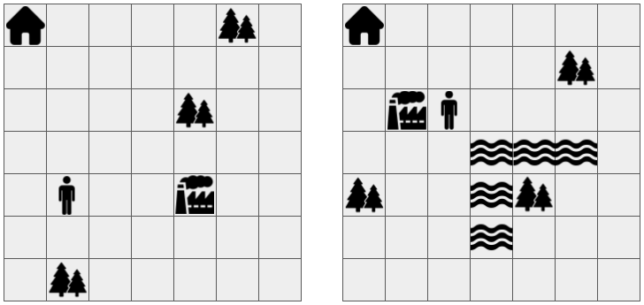
Q-value estimates generated through either of these methods can be used to bootstrap the learning process for the student. We evaluate our method on scenarios (such as that presented in Figure 1 where the student environment has features that were not present in the teacher task, demonstrating the robustness of the transferred knowledge to changing environmental conditions. Additionally, we argue that certain other automaton-based transfer methods might induce negative transfer in some scenarios. We demonstrate the efficacy of our proposed method in reducing training time, even when existing methods harm performance.

(a)                         (b)

Figure 1: Example environment configurations for the Blind Craftsman teacher (a) and student (b) environments, with additional obstacles introduced in the student environment.

Preliminaries

We assume that the teacher and student decision processes are non-Markovian Reward Decision Processes (NMRDP).

Definition 1 (Non-Markovian Reward Decision Process (NMRDP)).

An NMRDP is a decision process defined by the tuple $\mathcal{M}=\langle S,s_{0},A,T,R\rangle$, where $S$ is the set of valid states, $s_{0}\in S$ is the initial state, $A$ is the set of valid actions, $T:S\times A\times S\rightarrow[0,1]$ is a transition function defining transition probabilities for each state-action pair to every state in $S$, and $R:(S\times A)^{*}\rightarrow\mathbb{R}$ defines the reward signal observed at each time step based on the sequence of previously visited states and actions.

NMRDPs differ from MDPs in that the reward signal $R$ may depend on the entire history of observations, rather than only the current state. However, the reward signal is often a function of a set of abstract properties of the current state, which is of much smaller dimension than the original state space. Thus, it can be beneficial to represent the reward signal in terms of a simpler vocabulary defined over features extracted from the state. We assume the existence of a set of atomic propositions $AP$ for each environment which capture the dynamics of the reward function, as well as a labeling function $L:S\rightarrow 2^{AP}$ that translates experiences into truth assignments for each proposition $p\in AP$. In cases where such a labeling function does not explicitly exist, it is possible to find one automatically (Hasanbeig et al. 2021). Furthermore, we assume that the objectives in the teacher and student environments are identical and represented by the automaton $\mathcal{A}=(2^{AP},\Omega,\omega_{0},F,\delta)$ as defined below.

$\begin{matrix}\includegraphics[width=227.62204pt]{images/simple_env.png}\end{matrix}$
(a)                                   (b)

Figure 2: (a) A simple NMRDP. At each time step, the agent may move one square in any cardinal direction. A sequence of actions satisfies the objective iff the agent obtains both the sword and the shield. The objective is decomposed using the atomic propositions $AP=\{\text{sword},\text{shield}\}$, with a labeling function $L$ such that $L(s_{0})=\{\},L(s_{1})=\{\},L(s_{2})=\{\text{sword}\},L(s_{3})=\{\text{shield}\}$. Rollouts which achieve the objective also satisfy the LTL_f specification $\phi=\textbf{F}(\text{sword})\wedge\textbf{F}(\text{shield})$. (b) An automaton defined over the alphabet $\Sigma=\{\{\},\{\text{sword}\},\{\text{shield}\},\{\text{sword, shield}\}\}$. The automaton accepts the subset of strings in $\Sigma^{*}$ that satisfy the LTL_f formula.

Definition 2 (Deterministic Finite-State Automaton (DFA)).

A DFA is an automaton defined by the tuple $\mathcal{A}=\langle\Sigma,\Omega,\omega_{0},F,\delta\rangle$, where $\Sigma$ is the alphabet of the input language, $\Omega$ is the set of states with starting state $\omega_{0}$, $F\subseteq\Omega$ is the set of accepting states, and $\delta:\Omega\times\Sigma\rightarrow\Omega$ defines a state transition function.

The atomic propositions $AP$ comprise a vocabulary of abstract properties of the state space which directly correspond to the reward structure. Using the labeling function $L$, states in an NMRDP can be mapped to an element in the alphabet $\Sigma=2^{AP}$. Then, the set of rollouts which satisfy the objective constitute a regular language over $\Sigma$. The parameters $\Omega,\omega_{0},F,\delta$ are chosen such that the set of strings accepted by the objective automaton $\mathcal{A}$ is equivalent to the aforementioned regular language; we illustrate this with a simple example in Figure 2. An additional consequence of developing such a vocabulary is that RL objectives can be expressed as a regular language and subsequently converted into a DFA.

One benefit of the automaton representation is the ability to express non-Markovian reward signals in terms of the automaton state. During an episode, the state of the automaton can be computed in parallel with observations from the learning environment. Given the current automaton state $\omega$ and a new observation $s^{\prime}$, the new automaton state can be computed as $\omega^{\prime}=\delta(\omega,L(s^{\prime}))$. We assume that the atomic propositions capture the non-Markovian behavior of the reward signal; thus, the system dynamics are Markovian in the cross-product of the observation and automaton state spaces. Formally, we represent the cross-product of an NMRDP and its corresponding objective automaton as an MDP.

Definition 3 (Cross-Product Markov Decision Process).

The cross-product of an NMRDP $\mathcal{M}=\langle S,s_{0},A,T,R\rangle$ and a DFA $\mathcal{A}=\langle\Sigma,\Omega,\omega_{0},F,\delta\rangle$ which captures the non-Markovian behavior of the reward signal is a Markov Decision Process (MDP) $\mathcal{M}_{\text{prod}}=\langle S\times\Omega,(s_{0},\omega_{0}),A\times\Sigma,T\times\delta,R^{\prime}\rangle$ where $R^{\prime}:\Omega\times\Sigma\rightarrow\mathbb{R}$ is a Markovian reward signal (i.e., can be expressed as a function of only the current state and action).

Note that transforming an NMRDP into a cross-product MDP permits the use of traditional RL algorithms, which rely upon the Markovian assumption, for decision tasks with non-Markovian reward signals.

Implicit in the previous discussion is that the objective is translated into an automaton prior to learning. The difficulty of explicitly constructing an automaton to represent a desired objective has motivated the development of automated methods for converting a reward specification into an automaton representation. Such methods observe a correspondence between formal logics (such as regular expressions, LTL, and its variants) and finite-state automata (Wolper, Vardi, and Sistla 1983). In particular, finite-trace Linear Temporal Logic (LTL_f) has been used to represent RL objectives (Camacho et al. 2019; Velasquez et al. 2021).

Definition 4 (Finite-Trace Linear Temporal Logic (LTL_f)).

A formula in LTL_f consists of a set of atomic propositions $AP$ which are combined by the standard propositional operators and the following temporal operators: the next operator X$\phi$ ($\phi$ will be true in the next time step), the eventually operator F$\phi$ ($\phi$ will be true in some future time step), the always operator G$\phi$ ($\phi$ will be true in all future time steps), the until operator $\phi_{1}$ U $\phi_{2}$ ($\phi_{2}$ will be true in some future time step, and until then $\phi_{1}$ must be true), and the release operator $\phi_{1}$ R $\phi_{2}$ ($\phi_{2}$ must be true always or until $\phi_{1}$ first becomes true).

It has been shown that specifications in LTL_f can be transformed into an equivalent deterministic Büchi automaton (De Giacomo and Vardi 2015), and tools for compiling automata are readily available (Zhu et al. 2017). Moreover, it is possible, in principle, to convert descriptions using a predefined subset of natural language into LTL (Brunello, Montanari, and Reynolds 2019). Thus, it is feasible to translate a specification provided by a domain expert into an automaton representation using automated methods.

Automaton Distillation

In this section, we outline our strategy for transferring knowledge from a teacher to a student. Our method leverages a DQN oracle trained in the teacher environment and an automaton representation of the objective. Knowledge is first distilled from the teacher into the automaton, and then from the automaton into the student DQN during training. We term this methodology “automaton distillation”, as it entails distilling insights from a teacher automaton to enhance the learning of a student DQN. This approach stands in contrast to traditional policy distillation, where knowledge is directly transferred from the teacher DQN to the student DQN (Rusu et al. 2015).

Automaton distillation begins by training a teacher agent using Deep Q-learning. Subsequently, the teacher’s Q-values are distilled into the objective automaton, associating each transition’s value with an estimated Q-value for corresponding state-action pairs in the teacher environment. Then, a student agent undergoes training in the target environment, employing an adapted DQN loss function that incorporates the Q-values derived from the automaton.

Dynamic Transfer. Our primary focus lies in a dynamic transfer learning algorithm. This algorithm distills value estimates from an agent trained using Deep Q-learning into the objective automaton. This distillation is achieved through a contractive mapping from state-action pairs in the teacher NMRDP to the abstract MDP defined by the automaton. Additionally, an analogous expansive mapping from the abstract MDP to the student NMRDP provides an initial Q-value estimate for state-action pairs in the target domain, assisting the learning process of the student DQN. The automaton acts as a mediator between teacher and student domains, enabling experience sharing without requiring manual state-space mappings (Taylor and Stone 2005) or unsupervised map learning (Ammar et al. 2015).

The DQN loss function is given in Eq. (1), where $ER$ is an experience replay buffer with samples collected over the course of training, $U$ denotes the uniform distribution, $r$ is an immediate reward, $\gamma$ is a discount factor, and $Q(s,a;\theta)$ is the student DQN parameterized by $\theta$. The parameters $\theta^{\text{target}}$ are often taken from an old copy of the DQN in order to stabilize learning.

$$\mathrm{Loss}(\theta)=$$ (1)

$$\mathbb{E}_{(s,a,r,s^{\prime})\sim U(ER)}[(r+\gamma\max_{a^{\prime}}Q(s^{\prime},a^{\prime};\theta^{\text{target}})-Q(s,a;\theta))^{2}]$$

The teacher DQN is trained using only standard RL methods (Wang et al. 2016; Van Hasselt, Guez, and Silver 2016; Schaul et al. 2015). However, in order to track the current node in the automaton as well as the current state, we store samples of the form $((s,\omega),a,r,(s^{\prime},\omega^{\prime}))$ in the experience replay buffer $ER$. We define $\eta_{\text{teacher}}:\Omega\times\Sigma\to\mathbb{N}$ to be the number of times each automaton node $\omega$ and a set of atomic propositions $\sigma\in 2^{AP}$ appear in the experience replay $ER$ of the teacher (note that $\omega$ and $\sigma$ define a transition in the automaton objective as given by $\delta(\omega,\sigma)=\omega^{\prime}$):

$$\eta_{\text{teacher}}(\omega,\sigma)=|\{((s,\omega),a,r,(s^{\prime},\omega^{\prime}))\in ER|L(s^{\prime})=\sigma\}|.$$ (2)

Similarly, we define $Q^{\text{avg}}_{\text{teacher}}:\Omega\times\Sigma\rightarrow\mathbb{R}$ to be the average Q-value corresponding to the automaton transition given by $\omega$ and $\sigma\in 2^{AP}$, according to the teacher DQN.

$$Q^{\text{avg}}_{\text{teacher}}(\omega,\sigma)=\frac{\sum_{\{((s,\omega),a,r,(s^{\prime},\omega^{\prime}))\in ER|L(s^{\prime})=\sigma\}}Q_{\text{teacher}}(s,a)}{\eta_{\text{teacher}}(\omega,\sigma)}$$ (3)

We leverage the preceding equations to create a new loss function (shown in Eq. (4)) during student training whereby the average Q-values of the teacher corresponding to transitions in the automaton objective are pre-computed and used to bootstrap the learning process. Intuitively, using teacher Q-values to estimate the optimal value function during the early phases of training resolves the issue of poor initial value estimates, which causes slow convergence in standard RL algorithms. As we show in the experiments, this is an effective means of performing non-Markovian knowledge transfer since the automaton objective is a much lower-dimensional representation of the environment dynamics and encodes the non-Markovian reward signal.

$$\mathrm{Loss}(\theta)=$$ (4)

$$\mathbb{E}_{((s,\omega),a,r,(s^{\prime},\omega^{\prime}))\sim P(ER)}[\>\beta(\omega,L(s^{\prime}))Q^{\text{avg}}_{\text{teacher}}(\omega,L(s^{\prime}))+$$

$$(1-\beta(\omega,L(s^{\prime})))(r+\gamma\max_{a^{\prime}}Q(s^{\prime},a^{\prime};\theta^{\text{target}}))-Q(s,a;\theta)\>]^{2}$$

In the preceding equation, $P$ is a priority function which favors sampling high-error experiences and $\beta:\Omega\times\Sigma\rightarrow[0,1]$ is an annealing function that controls the importance of the initial Q-value estimate given by the automaton relative to the standard Q-learning update. We use $\beta(\omega,\sigma)=\rho^{\eta_{student}(\omega,\sigma)}$, where $\rho=0.999$ and $\eta_{student}(\omega,\sigma)$ represents how many times the automaton transition defined by $\omega$ and $\sigma$ has been previously sampled from the experience replay buffer while training the student.

Data: Teacher automaton Q-values $Q_{\text{teacher}}$, automaton state transition function $\delta$, labeling function $L$, number of training steps $T$, number of steps per target update $t_{\text{update}}$, batch size $M$, learning rate $\alpha$, discount factor $\gamma$, exploration constant $\epsilon$, annealing rate $\rho$

Result: Student DQN with parameters $\theta$

Initialize replay buffer $ER$, network parameters $\theta$, target network parameters $\theta_{\text{target}}$, automaton transition visit counts $\eta$;

for $t\leftarrow 1$ to $T$ do

       Take $\epsilon$-greedy action $a$ w.r.t. $Q((s,\omega),a;\theta)$, observing reward $r$ and new state $s^{\prime}$;

       Compute new automaton state $\omega^{\prime}=\delta(\omega,L(s^{\prime}))$;

       Append augmented experience $((s,\omega),a,r,(s^{\prime},\omega^{\prime}))$ to the replay buffer $ER$ with priority 1;

       Sample $M$ transitions from replay with priority $p_{i}$;

       Compute annealing parameters for each transition $\beta_{i}\leftarrow\rho^{\eta(\omega_{i},L(s^{\prime}_{i})}$;

       Generate adjusted targets $Q^{\prime}_{i}\leftarrow\beta_{i}Q_{\text{teacher}}(\omega_{i},L(s^{\prime}_{i}))+(1-\beta_{i})(r_{i}+\gamma\max_{a^{\prime}}Q((s^{\prime}_{i},\omega^{\prime}_{i}),a^{\prime};\theta_{\text{target}}))$;

       Update network parameters $\theta\leftarrow\theta+\frac{\alpha}{M}\sum_{i}p_{i}\nabla_{\theta}(Q^{\prime}_{i}-Q((s_{i},\omega_{i}),a_{i};\theta))^{2}$;

       Update buffer priorities $p_{i}=(Q^{\prime}_{i}-Q((s_{i},\omega_{i}),a_{i};\theta))^{2}$;

       for $i\leftarrow 1$ to $M$ do

             Update visit count $\eta(\omega_{i},L(s^{\prime}_{i}))\leftarrow\eta(\omega_{i},L(s^{\prime}_{i}))+1$;

            

       end for

      if $t=0\mod t_{\text{update}}$ then

             $\theta_{\text{target}}\leftarrow\theta$;

            

       end if

      

end for

Algorithm 1 DQN with Automaton Distillation

The asymptotic behavior of automaton Q-learning depends on $\beta$; when $\beta=0$, automaton Q-learning reduces to vanilla Q-Learning. We provide the following proof of convergence for tabular automaton Q-learning.

Theorem 1. The automaton Q-learning algorithm given by

$$Q_{t+1}(s_{t},a_{t})=(1-\alpha_{t})Q_{t}(s_{t},a_{t})$$ (5)

$$+\alpha_{t}(1-\beta_{t})(R(s_{t},a_{t})+\gamma V_{t}(s_{t+1}))$$

$$+\alpha_{t}\beta_{t}Q^{\text{avg}}_{\text{teacher}}(\omega,L(s_{t+1}))$$

converges to the optimal $Q^{*}(s,a)$ values if:

1. The state and action spaces are finite.

2. $\alpha_{t}\in[0,1)$, $\sum_{t}\alpha_{t}=\infty$ and $\sum_{t}\alpha^{2}_{t}<\infty$.

3. $\beta_{t}\geq 0$, $\lim\limits_{t\rightarrow\infty}\beta_{t}=0$, and $\sum_{t}\alpha_{t}(1-\beta_{t})=\infty$.

4. The variance $\operatorname{Var}(R(s,a))$ is bounded.

5. $\gamma=1$ and all policies lead to a cost-free terminal state; otherwise, $\gamma\in[0,1)$.

Proof: We decompose automaton Q-learning into two parallel processes $q$ and $r$ given by

$$q_{t+1}(s_{t},a_{t}) =(1-\alpha_{t})q_{t}(s_{t},a_{t})$$ (6)

$$+\alpha_{t}(1-\beta_{t})(R(s_{t},a_{t})+\gamma V_{t}(s_{t+1}))$$

$$r_{t+1}(s_{t},a_{t}) =(1-\alpha_{t})r_{t}(s_{t},a_{t})+\alpha_{t}\beta_{t}Q^{\text{avg}}_{\text{teacher}}(\omega,L(s_{t+1}))$$

such that $Q_{t}(s,a)=q_{t}(s,a)+r_{t}(s,a)$. The process $q$ corresponds to a modified version of Q-learning; using the same annealing function as in Equation 4, $q$ converges to the optimal Q-table $Q^{*}$ with probability (w.p.) 1 as shown in (Jaakkola, Jordan, and Singh 1993). To see that $r$ converges to 0 w.p. 1, we observe that $Q^{\text{avg}}_{\text{teacher}}(\omega,L_{s_{t+1}})$ is constant when training the student and so $r_{t}$ is a contraction whose fixed point occurs at

$$r_{t}(s_{t},a_{t})=\beta_{t}Q^{\text{avg}}_{\text{teacher}}(\omega,L(s_{t+1}))$$ (7)

Since $\lim\limits_{t\rightarrow\infty}\beta=0$, the fixed point of $r_{t}$ approaches 0 as $t\rightarrow\infty$. Thus, since $q$ and $r$ converge to $Q^{*}$ and $0$ respectively w.p. 1, their sum $Q$ converges to $Q^{*}$ w.p. 1. ∎

Static Transfer. Static value estimates can be effective when the abstract MDP defined by the automaton accurately captures the environment dynamics. Such estimates can be computed via tabular Q-learning over the abstract MDP:

$$Q(\omega,\sigma)\!\leftarrow\!Q(\omega,\sigma)+\alpha(R(\omega,\sigma)+\gamma\max_{\sigma^{\prime}}Q(\omega^{\prime},\sigma^{\prime})-Q(\omega,\sigma))\>.$$ (8)

The resulting Q-values can be used in the place of $Q^{\text{avg}}_{\text{teacher}}$ in Equation 4. This method has the benefit of stabilizing training in the early stages without requiring a DQN oracle or any additional information beyond the reward structure.

Related Work

Deep RL has made remarkable progress in many practical problems, such as recommendation systems, robotics, and autonomous driving. However, despite these successes, insufficient data and poor generalization remain open problems. In most real-world problems, it is difficult to obtain training data, so RL agents often learn with simulated data. However, RL agents trained with simulated data usually have poor performance when transferred to unknown environment dynamics in real-world data. To address these two challenges, transfer learning techniques (Zhu, Lin, and Zhou 2020) have been adopted to solve two RL tasks: 1) state representation transfer and 2) policy transfer.

Among transfer learning techniques, Domain Adaptation (DA) is the most well-studied in deep RL. Early attempts at DA construct a mapping from states and actions in the source domain onto the target domain by hand (Taylor and Stone 2005). Subsequent works aim to learn a set of general latent environment representations that can be transferred across different but similar domains. For example, a multi-stage agent, DisentAngled Representation Learning Agent (DARLA) (Higgins et al. 2017), proposed to learn a general representation by adding an internal layer of pre-trained Denosising AutoEncoder. With learned general representation in the source domain, the agent quickly learns a robust policy that produces decent performance on similar target domains without further tuning. However, DARLA cannot clearly define and separate domain-specific and domain-general features, and it causes performance degradation on some target tasks. Moreover, Contrastive Unsupervised Representations for Reinforcement Learning (Srinivas, Laskin, and Abbeel 2020) aimed to address this issue by integrating contrastive loss. Furthermore, Latent Unified State Representation (Xing et al. 2021) proposed a two-stage agent that can fully separate domain-general and domain-specific features by embedding both the forward loss and the reverse loss in Cycle-Consistent AutoEncoder (Jha et al. 2018).

Previous work has explored the use of high-level symbolic domain descriptions to construct a low-dimensional abstraction of the original state space (Kokel et al. 2022), which can be used to model the dynamics of the original system. (Icarte et al. 2022) further construct an automaton which realizes the abstract decision process and use the automaton to convey information about the reward signal.

Static transfer learning methods based on reward machines were developed in (Camacho et al. 2018; Icarte et al. 2022). By treating the nodes and edges in the automaton as states and actions respectively, the automaton can be transformed into a low-dimensional abstract MDP which can be solved using Q-learning or value iteration approaches. The solution to the abstract MDP can speed up learning in the original environment using a potential-based reward shaping function (Camacho et al. 2019) or by introducing counterfactual experiences during training (Icarte et al. 2022).

(a)                      (b)                      (c)

Figure 3: Example $7\times 7$ environment configurations for the Blind Craftsman (a), Dungeon Quest (b), and Diamond Mine (c) environments.

However, static transfer methods perform poorly when the abstract MDP fails to capture the behavior of the underlying process. Consider applying the static transfer approach proposed in (Icarte et al. 2022) for the objective defined by the LTL${}_{\text{f}}$ formula $\phi=\textbf{F}(\text{b}\vee\text{e})\wedge(\neg\textbf{F}(\text{a})\vee\neg\textbf{F}(\text{c}))\wedge(\text{a}\textbf{ R }\neg\text{b})\wedge(\text{c}\textbf{ R }\neg\text{d})\wedge(\text{d}\textbf{ R }\neg\text{e})$, whose automaton is given in Figure 4.

Figure 4: Simple automaton with two traces.

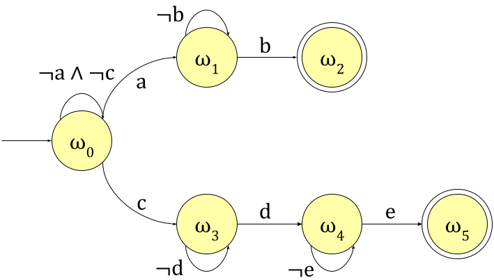
Assume that the reward function grants a reward of 1 for transitions leading to either terminal state and a reward of 0 for all other transitions. (Icarte et al. 2022) perform value iteration over the abstract MDP:

$$V(\omega):=\max_{\omega^{\prime}=\delta(\omega,\sigma)}R(\omega,\sigma)+\gamma V(\omega^{\prime})$$ (9)

In the automaton in Figure 4, there are two traces which satisfy the objective: one of length 2 and one of length 3. Due to the discount factor $\gamma<1$, value iteration will favor taking transition $a$, which has a shorter accepting path, over transition $c$ in the starting state. However, it may be the case that observing $b$ after observing $a$ takes many steps in the original environment, and thus the longer trace $c\rightarrow d\rightarrow e$ takes less steps to reach an accepting state.

In contrast to static transfer, which uses prior knowledge of the reward function to model the behavior of the target process, dynamic transfer leverages experience acquired by interaction in a related domain to empirically estimate the target value function. Dynamic transfer has the advantage of implicitly factoring in knowledge of the teacher environment dynamics; in the previous example, if the shorter trace $a\rightarrow b$ takes more steps in the teacher environment than the longer trace $c\rightarrow d\rightarrow e$, this will be reflected in the discounted value estimates learned by the teacher.

Experimental Results

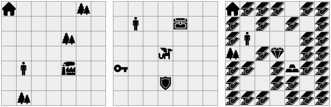
We evaluate both static and dynamic automaton distillation on various grid-world environments. We use a randomly generated $7\times 7$ instance of each grid-world environment as the source domain and an independently generated $10\times 10$ instance as the target domain. Agents are trained in parallel on $8$ environment instances. The layout of the grid-world is generated once for each environment instance and subsequently kept fixed across interaction episodes. In each grid-world environment, the objective is expressed as an LTL_f formula over atomic propositions defined for each environment. The objective is converted into an equivalent automaton representation which can be used for both source and target domains. The state space consists of the current location of the agent and all special tiles as well as the agent’s inventory. As an action, the agent may either move one square in any of the cardinal directions or interact with the tile the agent is currently standing on. The environments we use are described below (sample $7\times 7$ configurations for each environment can be seen in Figure 3).

Blind Craftsman: This environment consists of wood tiles, a factory tile, and a home tile. The agent can acquire wood by interacting with a wood tile (the agent may carry a maximum of two wood at a time) and craft a tool by interacting with a factory tile (one wood must be consumed to craft each tool). The objective is satisfied when the agent has crafted three tools and arrived home. Since the agent can only carry two wood at a time, the agent must alternate between collecting wood and crafting tools. The objective is defined over the atomic propositions $AP=\{\text{wood},\text{factory},\text{tools}\geq 3,\text{home}\}$ and given by the LTL_f formula $\phi=\textbf{G}(\text{wood}\implies\textbf{F}\text{ factory})\wedge\textbf{F}(\text{tools}\geq 3\text{ }\wedge\text{ home})$ with a corresponding automaton of 4 nodes and 12 transitions. The agent receives a reward of +1 for each wood collected and tool crafted, a reward of +100 for returning home with at least three tools, and a reward of -0.1 per time step.

Blind Craftsman with Obstacles: This environment is identical to the Blind Craftsman environment except that river tiles have been placed in fixed locations across the grid in the student environment. The agent is unable to traverse river tiles and must navigate around them; the river tiles are placed in such a way that all other tiles are still accessible.

Dungeon Quest: This environment consists of a key tile, a chest tile, a shield tile, and a dragon tile. The agent can acquire a key and a shield by interacting with a key or shield tile, respectively. Additionally, the agent can obtain a sword by interacting with a chest tile with a key in its inventory. Once the agent has the sword and the shield, it may interact with the dragon tile to defeat it and complete the objective. The objective is defined over the atomic propositions $AP=\{\text{key},\text{shield},\text{sword},\text{dragon}\}$ and given by the LTL_f formula $\phi=\textbf{F}(\text{dragon})\wedge(\text{key }\textbf{R }\neg\text{sword})\wedge(\text{sword }\textbf{R }\neg\text{dragon})\wedge(\text{shield }\textbf{R }\neg\text{dragon})$ with a corresponding automaton of 7 nodes and 17 transitions. The agent receives a reward of +1 for collecting each item, a reward of +100 for defeating the dragon, and a reward of -0.1 per time step.

(a)                                         (b)                                                 (c)

Figure 5: Objective automata for the Blind Craftsman (a), Dungeon Quest (b), and Diamond Mine environments.

Diamond Mine: This environment consists of a wood tile, a diamond tile, gold tiles, and iron tiles. The agent may acquire wood, iron, or gold by interacting with the respective tile. Once the agent has collected wood and 30 iron, it automatically crafts a pickaxe. The agent may then obtain diamond by interacting with the diamond tile while holding a pickaxe. Once the agent has acquired either 1 diamond or 10 gold, it may return to the home tile to complete the objective. To simplify the resulting automaton and limit unnecessary reward, once the agent has collected gold, it cannot obtain the diamond, and vice versa. Intuitively, although collecting diamond requires less automaton transitions, collecting 30 iron is relatively time-consuming. Thus, this environment represents a scenario where the objective automaton misrepresents the difficulty of the task. The objective is defined over the atomic propositions $AP=\{\text{wood},\text{diamond},\text{gold = 1},\text{gold = 2},...,\text{gold = 10},\text{home}\}$ and given by the LTL_f formula $\phi=\textbf{F}(\text{home})\wedge(\neg\textbf{F}(\text{gold}=1)\vee\neg\textbf{F}(\text{wood}))\wedge(\text{wood}\textbf{ R }\neg\text{diamond})\wedge(\text{gold = 1}\textbf{ R }\neg\text{gold = 2})\wedge...\wedge(\text{gold = 9}\textbf{ R }\neg\text{gold = 10})\wedge((\text{diamond}\vee\text{gold = 10})\textbf{ R }\neg\text{home})$ with a corresponding automaton of 15 nodes and 29 transitions. The agent receives rewards of +1 for collecting gold, +10 for collecting diamond, +100 for returning home, and -0.1 per time step.

Agents are trained for 2 million play steps or until convergence. Each agent is represented by a Dueling DQN (Wang et al. 2016), which consists of a convolutional feature extractor and separate value and advantage heads. The feature extractor is a residual network with 3 residual blocks, each using a $3\times 3$ convolutional kernel with 32 filters and Leaky ReLU activation. The resulting feature map is flattened and split into equal halves, which are fed separately to the value and advantage heads. Each head contains a single fully connected layer with 1 and $\#\text{ }actions$ nodes, respectively. Q-values are reconstructed by re-centering advantages to have a mean equal to the output of the value head.

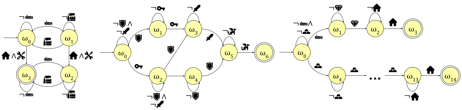
The network takes as input a stack of 2D grids, where each layer represents an entity type (either the agent, a tile type, or an inventory item type). Inventory items are represented by constant-valued input planes. Additionally, as in (Icarte et al. 2022), we incorporate the automaton state into the input, training on elements of the cross-product MDP state space $(s,\omega)\in S\times\Omega$. The objective automaton is generated using the Python FLLOAT synthesis tool based on the LTL_f behavioral specification; automata for each environment are shown in Figure 5. The automaton state is then tracked throughout each training episode and stored alongside each experience in the replay buffer. The automaton state is converted to a one-hot vector representation and concatenated to each half of the feature extractor output.

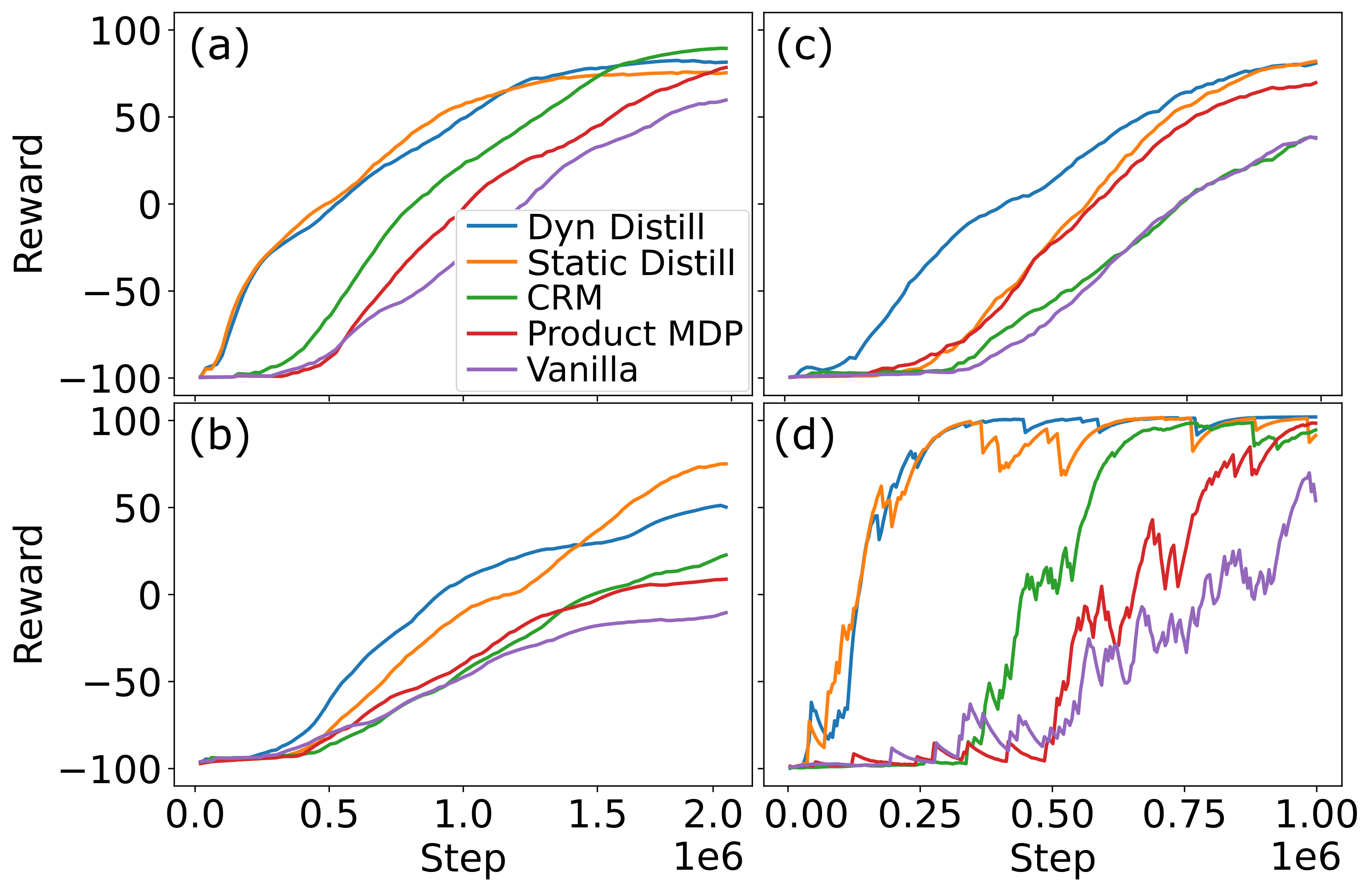
We evaluate the performance of static and dynamic automaton distillation against vanilla Q-learning in the student environment, Q-learning over the product MDP (i.e. including the automaton state in the DQN input), and CRM, a static transfer method proposed in (Icarte et al. 2022). Figure 7 shows the number of training steps required for each algorithm to converge to an optimal policy.

A primary use case for dynamic transfer occurs in the Diamond Mine environment, where the assumption that short automaton traces correlate with shorter trajectories in the original environment is misleading. Dynamic automaton distillation utilizes an empirical estimate of trajectory length over the teacher decision process, circumventing inaccuracies in the abstract MDP. Thus, dynamic automaton distillation is effective when the optimal policies in the teacher and student environments follow similar automaton traces.

Figure 6: Teacher Q-values produced by dynamic (red) and static (blue) automaton distillation on the Blind Craftsman environment. Transitions which were not observed in the environment are denoted by dotted lines.

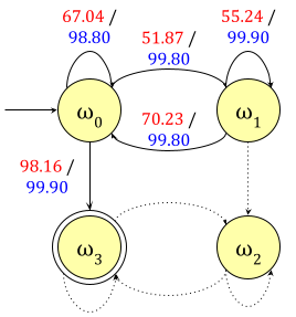
Some behavioral specifications can lead to objective automata with cycles, as evidenced by the Blind Craftsman environment. Figure 6 shows the Q-values generated by automaton distillation. Unlike static distillation, dynamic distillation can distinguish between states which are (nearly) equivalent in the abstract MDP by incorporating episode length; states which are further from the goal receive discounted rewards, resulting in smaller Q-values.

Cycles in the automaton do not necessarily lead to infinite reward loops - it is often the case that, in the original environment, the cycle may be taken only a finite number of times. While it is possible to construct an automaton without cycles by expanding the state space of the automaton to include the number of cycles taken, the maximum number of cycle traversals must be known a priori and incorporated into the objective specification, which may not be possible. Additionally, environments which share an objective may admit different numbers of cycle traversals; thus, cycles offer a compact representation which permits knowledge transfer between environments. However, the presence of cycles can aggravate the differences between the abstract MDP and original decision process, resulting in negative knowledge transfer. In such cases, state-of-the-art transfer methods (Icarte et al. 2022) may actually increase training time relative to a naïve learning algorithm.

Figure 7: Reward per episode (y-axis) over time (x-axis) during the course of training using dynamic automaton distillation (blue) vs. static automaton distillation (orange), CRM (green), Q-learning over the product MDP (red), and vanilla Q-learning (purple) on the Dungeon Quest (a), Diamond Mine (b) and Blind Craftsman (c) environments. Each line is an ensemble average over 20 trials. One trial of Blind Craftsman with Obstacles (see Figure 1) is shown in (d).

Conclusion

In this paper, we proposed automaton distillation, which leverages symbolic knowledge of the objective and reward structure in the form of formal language, to stabilize and expedite training of reinforcement learning agents. Value estimates for transitions in the automaton are generated using static (i.e. a priori) methods such as value iteration over an abstraction of the target domain or dynamically estimated by mapping experiences collected in a related source domain to automaton transitions. The resulting value estimates are used as initial learning targets to bootstrap the student learning process. We illustrate several failure cases of existing automaton-based transfer methods, which exclusively reason over a priori knowledge, and argue instead for the use of dynamic transfer. We demonstrate that both static and dynamic automaton distillation reduce training costs and outperform state-of-the-art knowledge transfer techniques.

References

- Ammar et al. (2015) Ammar, H. B.; Eaton, E.; Luna, J. M.; and Ruvolo, P. 2015. Autonomous cross-domain knowledge transfer in lifelong policy gradient reinforcement learning. In Twenty-fourth international joint conference on artificial intelligence.
- Anderson et al. (2020) Anderson, G.; Verma, A.; Dillig, I.; and Chaudhuri, S. 2020. Neurosymbolic reinforcement learning with formally verified exploration. Advances in neural information processing systems, 33: 6172–6183.
- Brunello, Montanari, and Reynolds (2019) Brunello, A.; Montanari, A.; and Reynolds, M. 2019. Synthesis of LTL formulas from natural language texts: State of the art and research directions. In 26th International Symposium on Temporal Representation and Reasoning (TIME 2019). Schloss Dagstuhl-Leibniz-Zentrum fuer Informatik.
- Camacho et al. (2018) Camacho, A.; Chen, O.; Sanner, S.; and McIlraith, S. A. 2018. Non-Markovian rewards expressed in LTL: Guiding search via reward shaping (extended version). In GoalsRL, a workshop collocated with ICML/IJCAI/AAMAS.
- Camacho et al. (2019) Camacho, A.; Icarte, R. T.; Klassen, T. Q.; Valenzano, R. A.; and McIlraith, S. A. 2019. LTL and Beyond: Formal Languages for Reward Function Specification in Reinforcement Learning. In IJCAI, volume 19, 6065–6073.
- De Giacomo and Vardi (2015) De Giacomo, G.; and Vardi, M. 2015. Synthesis for LTL and LDL on finite traces. In Twenty-Fourth International Joint Conference on Artificial Intelligence.
- Hasanbeig et al. (2021) Hasanbeig, M.; Jeppu, N. Y.; Abate, A.; Melham, T.; and Kroening, D. 2021. Deepsynth: Automata synthesis for automatic task segmentation in deep reinforcement learning. In Proceedings of the AAAI Conference on Artificial Intelligence, volume 35, 7647–7656.
- Higgins et al. (2017) Higgins, I.; Pal, A.; Rusu, A.; Matthey, L.; Burgess, C.; Pritzel, A.; Botvinick, M.; Blundell, C.; and Lerchner, A. 2017. DARLA: Improving zero-shot transfer in reinforcement learning. In International Conference on Machine Learning, 1480–1490. PMLR.
- Icarte et al. (2022) Icarte, R. T.; Klassen, T. Q.; Valenzano, R.; and McIlraith, S. A. 2022. Reward machines: Exploiting reward function structure in reinforcement learning. Journal of Artificial Intelligence Research, 73: 173–208.
- Jaakkola, Jordan, and Singh (1993) Jaakkola, T.; Jordan, M.; and Singh, S. 1993. Convergence of stochastic iterative dynamic programming algorithms. Advances in neural information processing systems, 6.
- Jha et al. (2018) Jha, A. H.; Anand, S.; Singh, M.; and Veeravasarapu, V. R. 2018. Disentangling factors of variation with cycle-consistent variational auto-encoders. In Proceedings of the European Conference on Computer Vision (ECCV), 805–820.
- Kokel et al. (2022) Kokel, H.; Prabhakar, N.; Ravindran, B.; Blasch, E.; Tadepalli, P.; and Natarajan, S. 2022. Hybrid Deep RePReL: Integrating Relational Planning and Reinforcement Learning for Information Fusion. In 2022 25th International Conference on Information Fusion (FUSION), 1–8. IEEE.
- Rusu et al. (2015) Rusu, A. A.; Colmenarejo, S. G.; Gulcehre, C.; Desjardins, G.; Kirkpatrick, J.; Pascanu, R.; Mnih, V.; Kavukcuoglu, K.; and Hadsell, R. 2015. Policy distillation. arXiv preprint arXiv:1511.06295.
- Schaul et al. (2015) Schaul, T.; Quan, J.; Antonoglou, I.; and Silver, D. 2015. Prioritized experience replay. arXiv preprint arXiv:1511.05952.
- Srinivas, Laskin, and Abbeel (2020) Srinivas, A.; Laskin, M.; and Abbeel, P. 2020. Curl: Contrastive unsupervised representations for reinforcement learning. arXiv preprint arXiv:2004.04136.
- Taylor and Stone (2005) Taylor, M. E.; and Stone, P. 2005. Behavior transfer for value-function-based reinforcement learning. In Proceedings of the fourth international joint conference on Autonomous agents and multiagent systems, 53–59.
- Tran and Garcez (2016) Tran, S. N.; and Garcez, A. S. d. 2016. Deep logic networks: Inserting and extracting knowledge from deep belief networks. IEEE transactions on neural networks and learning systems, 29(2): 246–258.
- Van Hasselt, Guez, and Silver (2016) Van Hasselt, H.; Guez, A.; and Silver, D. 2016. Deep reinforcement learning with double q-learning. In Proceedings of the AAAI conference on artificial intelligence, volume 30.
- Velasquez et al. (2021) Velasquez, A.; Bissey, B.; Barak, L.; Beckus, A.; Alkhouri, I.; Melcer, D.; and Atia, G. 2021. Dynamic Automaton-Guided Reward Shaping for Monte Carlo Tree Search. In Proceedings of the AAAI Conference on Artificial Intelligence, volume 35, 12015–12023.
- Verma et al. (2018) Verma, A.; Murali, V.; Singh, R.; Kohli, P.; and Chaudhuri, S. 2018. Programmatically interpretable reinforcement learning. In International Conference on Machine Learning, 5045–5054. PMLR.
- Wang et al. (2016) Wang, Z.; Schaul, T.; Hessel, M.; Hasselt, H.; Lanctot, M.; and Freitas, N. 2016. Dueling network architectures for deep reinforcement learning. In International conference on machine learning, 1995–2003. PMLR.
- Wolper, Vardi, and Sistla (1983) Wolper, P.; Vardi, M. Y.; and Sistla, A. P. 1983. Reasoning about infinite computation paths. In 24th Annual Symposium on Foundations of Computer Science (sfcs 1983), 185–194. IEEE.
- Xing et al. (2021) Xing, J.; Nagata, T.; Chen, K.; Zou, X.; Neftci, E.; and Krichmar, J. L. 2021. Domain adaptation in reinforcement learning via latent unified state representation. In Proceedings of the AAAI Conference on Artificial Intelligence, volume 35, 10452–10459.
- Zhu et al. (2017) Zhu, S.; Tabajara, L. M.; Li, J.; Pu, G.; and Vardi, M. Y. 2017. Symbolic ltlf synthesis. arXiv preprint arXiv:1705.08426.
- Zhu, Lin, and Zhou (2020) Zhu, Z.; Lin, K.; and Zhou, J. 2020. Transfer learning in deep reinforcement learning: A survey. arXiv preprint arXiv:2009.07888.