Outlier-robust additive matrix decomposition

Abstract

We study least-squares trace regression when the parameter is the sum of a $r$-low-rank matrix and a $s$-sparse matrix and a fraction $\epsilon$ of the labels is corrupted. For subgaussian distributions and feature-dependent noise, we highlight three needed design properties, each one derived from a different process inequality: a “product process inequality”, “Chevet’s inequality” and a “multiplier process inequality”. These properties handle, simultaneously, additive decomposition, label contamination and design-noise interaction. They imply the near-optimality of a tractable estimator with respect to the effective dimensions $d_{\operatorname*{\tiny{eff}},r}$ and $d_{\operatorname*{\tiny{eff}},s}$ of the low-rank and sparse components, $\epsilon$ and the failure probability $\delta$. The near-optimal rate is $\mathsf{r}(n,d_{\operatorname*{\tiny{eff}},r})+\mathsf{r}(n,d_{\operatorname*{\tiny{eff}},s})+\sqrt{(1+\log(1/\delta))/n}+\epsilon\log(1/\epsilon),$ where $\mathsf{r}(n,d_{\operatorname*{\tiny{eff}},r})+\mathsf{r}(n,d_{\operatorname*{\tiny{eff}},s})$ is the optimal rate in average with no contamination. Our estimator is adaptive to $(s,r,\epsilon,\delta)$ and, for fixed absolute constant $c>0$, it attains the mentioned rate with probability $1-\delta$ uniformly over all $\delta\geq\exp(-cn)$. Without matrix decomposition, our analysis also entails optimal bounds for a robust estimator adapted to the noise variance. Our estimators are based on “sorted” versions of Huber’s loss. We present simulations matching the theory. In particular, it reveals the superiority of “sorted” Huber’s losses over the classical Huber’s loss.

1 Introduction

Outlier-robust estimation has been a topic studied for many decades since the seminal work by Huber [49]. One of the objectives of the field is to device estimators which are less sensitive to outlier contamination. The formalization of outlyingness and the construction of robust estimators matured in several directions. One common assumption is that the adversary can only change a fraction $\epsilon$ of the original sample. For an extensive overview we refer, e.g., to [45, 62, 50] and references therein.

Within a very general framework, the minimax optimality of several robust estimation problems has been recently obtained in a series of elegant works by [15, 16, 44]. The construction, however, is based on Tukey’s depth, a hard computational problem in higher dimensions. A recent trend of research, initiated by [32, 55], has focused on the optimality of robust estimators within computationally tractable algorithms. The oblivious model assumes the contamination is independent of the original sample. In the adversarial model, the outliers may depend arbitrarily on the sample. For instance, optimal mean estimators for the adversarial model can now be computed in nearly-linear time [21, 38, 30, 28]. We refer to [33] for an extensive survey.

In the realm of robust linear regression, two broad lines of investigations exist: (1) one in which only the response (label) is contaminated and (2) the more general setting in which the covariates (features) are also corrupted [34, 36]. Model (1), albeit less general, has been considered in many applications and studied in numerous past and recent works [12, 59, 82, 43, 74, 35]. It has also some connection with the problems of robust matrix completion [13, 19, 17, 59, 52] and matrix decomposition [14, 13, 91, 48, 2]. Both models (1)-(2) have been considered assuming adversarial or oblivious contamination. For instance, an interesting property of model (1) with oblivious contamination is the existence of consistent estimators, a property not shared by the adversary model. See for instance [85, 8, 82, 43, 74].

In this work, we consider a new model: robust trace regression with additive matrix decomposition (RTRMD). It corresponds to least-squares trace regression when the parameter is the sum of a low-rank matrix and a sparse matrix and, simultaneously, the labels are adversarially contaminated. We assume there are at most $o$ outliers and the sample size $n$ is much smaller than the extrinsic dimension $p$. We focus on subgaussian distributions and pay attention to the following points:

• Adversarial label corruption in high dimensions. The parameter is a $d_{1}\times d_{2}$ matrix and $n\ll p:=d_{1}d_{2}$. RTRMD includes, as particular cases, $s$-sparse linear regression [84] and noisy $r$-low-rank matrix sensing [68]. One practical appeal of the established theory of high-dimensional estimation is the existence of efficient estimators adapted to $(s,r)$ — without resorting to Lepski’s method. Likewise, we assume no knowledge of $(s,r,o)$.

• Noise heterogeneity. The majority of the literature on (robust) least-squares regression, within the framework of $M$-estimation with decomposable regularizers [69], assumes feature-independent noise. We avoid this assumption and identify design properties and concentration inequalities needed for this case. See Section 9 for a discussion.

• Subgaussian rates and uniform confidence level. Minimax rates are defined on average or as a function of the failure probability $\delta$. For instance, the first seminal bounds in sparse linear regression were of the form $\sqrt{s\log(p/s\delta)/n}$ — optimal in average but suboptimal in $\delta$. The optimal rate is the “subgaussian” rate $\sqrt{s\log(p/s)/n}+\sqrt{\log(1/\delta)/n}$ — for which $\log(1/\delta)$ does not multiply the “effective dimension”. A second point is to what extent the estimator depends on $\delta$. Let $c>0$ be an absolute constant. Without knowing $\delta$, is there an estimator that “automatically” attains the optimal rate across all $\delta\geq\exp(-cn)$ with probability at least $1-\delta$? For sparse linear regression, [6] was the first to answer these points affirmatively when the noise is independent of the features. We ask the same questions for the general model RTRMD in case the noise is feature-dependent. See Section 9 for a discussion.

• Matrix decomposition. It is considered in [89, 14, 13, 91, 48, 63] assuming the “incoherence” condition and in [2] assuming the milder “low-spikeness” condition. See also Chapter 7 of the book [47]. These works do not consider label contamination. A general framework is proposed in [2] assuming a specific design property (see their Definition 2). In the applications considered in [2], this property is straightforwardly satisfied: either the design is the identity or the fixed design is invertible. For instance, multi-task learning has an invertible design in high dimensions (one has $n\geq d_{1}$ albeit $n\ll d_{1}d_{2}$). In this regard, trace regression with additive matrix decomposition is fundamentally a different model: with high probability, the random design is singular in the regime $n\ll d_{1}d_{2}$. To our knowledge, there is currently no optimal statistical theory for RTRMD — even without label contamination. Under assumptions (a)-(c), this work identifies three design properties to prove optimality for this problem: $\operatorname*{PP}$, $\operatorname*{IP}$ and $\operatorname*{MP}$. Respectively, each one is derived from a different process inequality: a “product process inequality”, “Chevet’s inequality” and a “multiplier process inequality”. See Sections 6.3 and 8.

The rest of the paper is organized as follows. We start presenting some useful notation. Section 2 states our general framework, Section 3 presents our estimators and Section 4 exemplifies with concrete models. Section 5 state new results for these models. It also presents reference to later sections concerning technical contributions. In Section 6, we review related literature and compare with our results. In Section 7, we state two concentration inequalities for the multiplier and product processes. In Section 8, we state our needed design properties and apply these inequalities to prove them. Section 9 presents a preliminary discussion. Sections 10-11 presents the proofs of our main results, namely, Theorems 15 and 21. Finally, Sections 12 and 13 finish with simulations and a final discussion. Additional proofs are presented in the Supplemental Material.

Notation.

We set $\mathds{R}^{p}:=\mathbb{R}^{d_{1}\times d_{2}}$. For a vector $\boldsymbol{v}$, $\|\boldsymbol{v}\|_{k}$ denotes its $\ell_{k}$-norm ($1\leq k\leq\infty$) and $\|\boldsymbol{v}\|_{0}$ is the number of its nonzero entries. We use similar notation for matrices (considered as vectors). We denote the Frobenius norm by $\|\cdot\|_{F}$, the nuclear norm by $\|\cdot\|_{N}$ and the operator norm by $\|\cdot\|_{\operatorname*{op}}$. Given norm $\mathcal{R}$ and $\mathbf{V}\in\mathds{R}^{p}\setminus\{0\}$, $\Psi_{\mathcal{R}}(\mathbf{V}):=\nicefrac{{\mathcal{R}(\mathbf{V})}}{{\|\mathbf{V}\|_{F}}}.$ The inner product in $\mathds{R}^{p}$ will be denoted by $\langle\mathchoice{{}\mkern-4.5mu}{{}\mkern-4.5mu}{{}\mkern-2.5mu}{}\langle\mathbf{V},\mathbf{W}\rangle\mathchoice{{}\mkern-4.5mu}{{}\mkern-4.5mu}{{}\mkern-2.5mu}{}\rangle=\mathsf{tr}(\mathbf{V}^{\top}\mathbf{W})$. For vectors, we use the notation $\langle\cdot,\cdot\rangle$. If $a\leq Cb$ for some absolute constant $C>0$, we write $a\lesssim b$ or $a\leq\mathcal{O}(b)$. We write $a\asymp b$ if $a\lesssim b$ and $b\lesssim a$. Given $\ell\in\mathbb{N}$, $[\ell]:=\{1,\ldots,\ell\}$. The $\psi_{2}$-Orlicz norm will be denoted by $|\cdot|_{\psi_{2}}$. Throughout the paper, given $\ell\in\mathbb{N}$, $A^{(\ell)}:=A/\sqrt{\ell}$ whenever $A$ is a number, vector or function.

We now recall the definition of the Slope norm [11]. Given nonincreasing positive sequence $\boldsymbol{\omega}:=\{\omega_{i}\}_{i\in[n]}$, the Slope norm at a point $\boldsymbol{u}\in\mathbb{R}^{n}$ is defined by $\|\boldsymbol{u}\|_{\sharp}:=\sum_{i\in[n]}\omega_{i}\boldsymbol{u}_{i}^{\sharp},$ where $\boldsymbol{u}_{1}^{\sharp}\geq\ldots\geq\boldsymbol{u}_{n}^{\sharp}$ denotes the nonincreasing rearrangement of the absolute coordinates of $\boldsymbol{u}$. Throughout this paper, unless otherwise stated, $\boldsymbol{\omega}\in\mathbb{R}^{n}$ will be the sequence with coordinates $\omega_{i}=\sqrt{\log(An/i)}$ for some $A\geq 2$. Recall that $\Omega:=\{\sum_{i=1}^{o}\omega_{i}^{2}\}^{1/2}\asymp o\log(n/o)$ [6]. With some abuse of notation, $\|\cdot\|_{\sharp}$ will also denote the Slope norm in $\mathbb{R}^{p}$ with sequence $\bar{w}_{j}=\sqrt{\log(\bar{A}p/j)}$ for some $\bar{A}\geq 2$.

$\mathbf{X}\in\mathds{R}^{p}$ will denote a random matrix with distribution $\Pi$ and covariance operator $\mathfrak{S}$ — seen as a vector, $\boldsymbol{\Sigma}$ is its covariance matrix. Given $[\mathbf{V},\mathbf{W},\boldsymbol{u}]\in(\mathds{R}^{p})^{2}\times\mathbb{R}^{n}$, we define the bilinear form $\langle\mathchoice{{}\mkern-4.5mu}{{}\mkern-4.5mu}{{}\mkern-2.5mu}{}\langle\mathbf{V},\mathbf{W}\rangle\mathchoice{{}\mkern-4.5mu}{{}\mkern-4.5mu}{{}\mkern-2.5mu}{}\rangle_{\Pi}:=\mathbb{E}[\langle\mathchoice{{}\mkern-4.5mu}{{}\mkern-4.5mu}{{}\mkern-2.5mu}{}\langle\mathbf{X},\mathbf{V}\rangle\mathchoice{{}\mkern-4.5mu}{{}\mkern-4.5mu}{{}\mkern-2.5mu}{}\rangle\langle\mathchoice{{}\mkern-4.5mu}{{}\mkern-4.5mu}{{}\mkern-2.5mu}{}\langle\mathbf{X},\mathbf{W}\rangle\mathchoice{{}\mkern-4.5mu}{{}\mkern-4.5mu}{{}\mkern-2.5mu}{}\rangle]=\langle\mathchoice{{}\mkern-4.5mu}{{}\mkern-4.5mu}{{}\mkern-2.5mu}{}\langle\mathfrak{S}(\mathbf{V}),\mathbf{W}\rangle\mathchoice{{}\mkern-4.5mu}{{}\mkern-4.5mu}{{}\mkern-2.5mu}{}\rangle$ and the pseudo-norms $\|\mathbf{V}\|_{\Pi}:=\langle\mathchoice{{}\mkern-4.5mu}{{}\mkern-4.5mu}{{}\mkern-2.5mu}{}\langle\mathbf{V},\mathbf{V}\rangle\mathchoice{{}\mkern-4.5mu}{{}\mkern-4.5mu}{{}\mkern-2.5mu}{}\rangle_{\Pi}^{1/2}$, $\|[\mathbf{V},\mathbf{W},\boldsymbol{u}]\|_{\Pi}:=\{\|\mathbf{V}\|_{\Pi}^{2}+\|\mathbf{W}\|_{\Pi}^{2}+\|\boldsymbol{u}\|_{2}^{2}\}^{1/2}$, $\|[\mathbf{V},\mathbf{W}]\|_{\Pi}:=\|[\mathbf{V},\mathbf{W},\mathbf{0}]\|_{\Pi}$ and $\|[\mathbf{V},\boldsymbol{u}]\|_{\Pi}:=\|[\mathbf{V},\mathbf{0},\boldsymbol{u}]\|_{\Pi}$. Given $\mathbb{C}\subset\mathds{R}^{p}$, let $\mu(\mathbb{C}):=\sup_{\mathbf{V}\in\mathbb{C}}\nicefrac{{\|\mathbf{V}\|_{F}}}{{\|\mathbf{V}\|_{\Pi}}}.$ Next, we define the unit balls $\mathbb{B}_{\Pi}:=\{\mathbf{V}\in\mathds{R}^{p}:\|\mathbf{V}\|_{\Pi}\leq 1\},$ $\mathbb{B}_{F}:=\{\mathbf{V}\in\mathds{R}^{p}:\|\mathbf{V}\|_{F}\leq 1\},$ $\mathbb{B}_{\ell}^{k}:=\{\boldsymbol{v}\in\mathbb{R}^{k}:\|\boldsymbol{v}\|_{\ell}\leq 1\}$ and, for given norm $\mathcal{R}$ in $\mathbb{R}^{k}$, $\mathbb{B}_{\mathcal{R}}:=\{\boldsymbol{v}:\mathcal{R}(\boldsymbol{v})\leq 1\}$. All the corresponding unit spheres will take the symbol $\mathbb{S}$. Finally, the Gaussian width of a compact set $\mathcal{B}\subset\mathbb{R}^{k\times\ell}$ is the quantity $\mathscr{G}(\mathcal{B}):=\mathbb{E}[\sup_{\mathbf{V}\in\mathcal{B}}\langle\mathchoice{{}\mkern-4.5mu}{{}\mkern-4.5mu}{{}\mkern-2.5mu}{}\langle\mathbf{V},\boldsymbol{\Xi}\rangle\mathchoice{{}\mkern-4.5mu}{{}\mkern-4.5mu}{{}\mkern-2.5mu}{}\rangle],$ where $\boldsymbol{\Xi}\in\mathbb{R}^{k\times\ell}$ is random matrix with iid $\mathcal{N}(0,1)$ entries.

2 General framework

Assumption 1 (Adversarial label contamination).

Let $\{(y_{i}^{\circ},\mathbf{X}_{i}^{\circ})\}_{i\in[n]}$ be an iid copy of a feature-label pair $(\mathbf{X},y)\in\mathds{R}^{p}\times\mathbb{R}$. We assume available a sample $\{(y_{i},\mathbf{X}_{i})\}_{i\in[n]}$ such that $\mathbf{X}_{i}=\mathbf{X}_{i}^{\circ}$ for all $i\in[n]$ and at most $o$ arbitrary outliers modify the label sample $\{y_{i}^{\circ}\}_{i\in[n]}$.

Letting $\boldsymbol{y}=(y_{i})_{i\in[n]}$, our underlying model is

$$\boldsymbol{y}=\boldsymbol{f}+\sqrt{n}\boldsymbol{\theta}^{*}+\boldsymbol{\xi},$$ (1)

where $\boldsymbol{f}:=(f_{i})_{i\in[n]}$ and $\boldsymbol{\xi}:=(\xi_{i})_{i\in[n]}$ are, respectively, iid copies of unknown random variables $f,\xi\in\mathbb{R}$ and $\boldsymbol{\theta}^{*}\in\mathbb{R}^{n}$ is an arbitrary unknown vector with at most $o$ nonzero coordinates. We assume $\xi$ and $\mathbf{X}$ are centered and $\mathbb{E}[\xi\mathbf{X}]=0$. The number $\epsilon:=o/n$ is referred as the “contamination fraction”.

Define the design operator $\mathfrak{X}:\mathds{R}^{p}\rightarrow\mathbb{R}^{n}$ with components $\mathfrak{X}_{i}(\mathbf{V}):=\langle\mathchoice{{}\mkern-4.5mu}{{}\mkern-4.5mu}{{}\mkern-2.5mu}{}\langle\mathbf{X}_{i},\mathbf{V}\rangle\mathchoice{{}\mkern-4.5mu}{{}\mkern-4.5mu}{{}\mkern-2.5mu}{}\rangle$. In its general form, our goal is to estimate $\boldsymbol{f}$ assuming that, for some $[\mathbf{B},\boldsymbol{\Gamma}]\in\mathds{R}^{p}$, the average approximation error $(\nicefrac{{1}}{{n}})\|\mathfrak{X}(\mathbf{B}+\boldsymbol{\Gamma})-\boldsymbol{f}\|_{2}^{2}$ is “small”. To be precise, assuming $\epsilon\leq c$ for some constant $c\in(0,1/2)$, we would like to design an estimator $[\hat{\mathbf{B}},\hat{\boldsymbol{\Gamma}}]$ satisfying, with probability at least $1-\delta$, “oracle inequalities” of the form

$$\|\mathfrak{X}^{(n)}(\hat{\mathbf{B}}+\hat{\boldsymbol{\Gamma}})-\boldsymbol{f}^{(n)}\|_{2}^{2}\leq\inf_{[\mathbf{B},\boldsymbol{\Gamma}]\in\mathcal{F}}\left\{C\|\mathfrak{X}^{(n)}(\mathbf{B}+\boldsymbol{\Gamma})-\boldsymbol{f}^{(n)}\|_{2}^{2}+r_{\mathbf{B},\boldsymbol{\Gamma}}(n,d_{\operatorname*{\tiny{eff}}},\epsilon,\delta)\right\}.$$ (2)

In above, $C\approx 1$ is an universal constant, $\mathcal{F}$ is a class of parameters associated to well known parsimonious properties — e.g, sparsity or low-rankness — and $r_{\mathbf{B},\boldsymbol{\Gamma}}(n,d_{\operatorname*{\tiny{eff}}},\epsilon,\delta)$ is an appropriate rate that depends on the “effective dimension” $d_{\operatorname*{\tiny{eff}}}$ of $\mathcal{F}$. In Section 5, we specify different classes of interest, each associated to the examples of Section 4.

When the model is “well-specified”, there is $[\mathbf{B}^{*},\boldsymbol{\Gamma}^{*}]\in\mathcal{F}$ such that

$$[\mathbf{B}^{*},\boldsymbol{\Gamma}^{*}]\in\operatorname*{argmin}_{[\mathbf{B},\boldsymbol{\Gamma}]\in(\mathds{R}^{p})^{2}}\mathbb{E}\left[y-\langle\mathchoice{{}\mkern-4.5mu}{{}\mkern-4.5mu}{{}\mkern-2.5mu}{}\langle\mathbf{X},\mathbf{B}+\boldsymbol{\Gamma}\rangle\mathchoice{{}\mkern-4.5mu}{{}\mkern-4.5mu}{{}\mkern-2.5mu}{}\rangle\right]^{2}.$$ (3)

This corresponds to (1) with $f:=\langle\mathchoice{{}\mkern-4.5mu}{{}\mkern-4.5mu}{{}\mkern-2.5mu}{}\langle\mathbf{X},\mathbf{B}^{*}+\boldsymbol{\Gamma}^{*}\rangle\mathchoice{{}\mkern-4.5mu}{{}\mkern-4.5mu}{{}\mkern-2.5mu}{}\rangle$. In this case, $\|\mathfrak{X}^{(n)}(\mathbf{B}^{*}+\boldsymbol{\Gamma}^{*})-\boldsymbol{f}^{(n)}\|_{2}=0$, Assumption 1 and (1) are equivalent and the rate $r_{\mathbf{B}^{*},\boldsymbol{\Gamma}^{*}}(n,d_{\operatorname*{\tiny{eff}}},\epsilon,\delta)$ is the minimax optimal rate for the well-specified model. More broadly, our goal is to obtain, under the assumptions discussed in the introduction, inequalities of the form (2), ensuring optimal statistical guarantees for least-squares trace regression in presence of either additive matrix decomposition, label contamination or inexact parsimony.

3 Our estimators

Our estimators are based on the following class of losses.

These losses are convex. For instance, when $q=2$, $\rho_{\tau\boldsymbol{\omega},2}$ is the optimal value of the problem defining the proximal mapping of $\tau\|\cdot\|_{\sharp}$. When $\omega_{1}=\ldots=\omega_{n}=1$, separability implies the explicit expression:

$$\mathcal{L}_{\tau\boldsymbol{\omega},2}(\mathbf{B})=\tau^{2}\sum_{i=1}^{n}\Phi\left(\frac{y_{i}-\mathfrak{X}_{i}(\mathbf{B})}{\tau\sqrt{n}}\right),$$ (4)

where $\Phi:\mathbb{R}\rightarrow\mathbb{R}$ is the Huber’s function $\Phi(t)=\min\{(\nicefrac{{1}}{{2}})t^{2},|t|-\nicefrac{{1}}{{2}}\}$. Thus, Huber regression corresponds to $M$-estimation with the loss $\mathcal{L}_{\tau\boldsymbol{\omega},2}$ with constant weighting sequence $\boldsymbol{\omega}$. In this work we advocate the use of the loss $\mathcal{L}_{\tau\boldsymbol{\omega},2}$ with varying weights. Throughout this paper, we fix the sequence $\boldsymbol{\omega}:=(\omega_{i})_{i\in[n]}$ to be $\omega_{i}:=\sqrt{\log(An/i)}$ for some $A\geq 2$. It corresponds to a “Sorted” generalization of Huber’s loss.

In high-dimensions, we additionally use regularization norms $(\mathcal{R},\mathcal{S})$. We consider the estimator

$$\begin{array}[]{ccl}[\hat{\mathbf{B}},\hat{\boldsymbol{\Gamma}}]&\in&\operatorname*{argmin}_{[\mathbf{B},\boldsymbol{\Gamma}]\in(\mathds{R}^{p})^{2}}\mathcal{L}_{\tau\boldsymbol{\omega},2}(\mathbf{B}+\boldsymbol{\Gamma})+\lambda\mathcal{R}(\mathbf{B})+\chi\mathcal{S}(\boldsymbol{\Gamma})\\ &&\mbox{s.t.}\quad\|\mathbf{B}\|_{\infty}\leq\mathsf{a},\end{array}$$ (7)

where $\lambda,\chi,\tau>0$ and $\mathsf{a}\in(0,\infty]$ are tuning parameters. If we are not concerned with matrix decomposition, we instead consider, for $q\in\{1,2\}$, estimators of the form

$$\begin{array}[]{ccl}\hat{\mathbf{B}}&\in&\operatorname*{argmin}_{\mathbf{B}\in\mathds{R}^{p}}\mathcal{L}_{\tau\boldsymbol{\omega},q}(\mathbf{B})+\lambda\mathcal{R}(\mathbf{B}).\end{array}$$ (9)

By adding an extra variable $\hat{\boldsymbol{\theta}}$ — aiming in estimating the nuisance parameter $\boldsymbol{\theta}^{*}$ — the solution of (7) can be equivalently found solving

$$\begin{array}[]{ccl}&&\min_{[\mathbf{B},\boldsymbol{\Gamma},\boldsymbol{\theta}]\in(\mathds{R}^{p})^{2}\times\mathbb{R}^{n}}\frac{1}{2n}\sum_{i=1}^{n}\left(y_{i}-\langle\mathchoice{{}\mkern-4.5mu}{{}\mkern-4.5mu}{{}\mkern-2.5mu}{}\langle\mathbf{X}_{i},\mathbf{B}+\boldsymbol{\Gamma}\rangle\mathchoice{{}\mkern-4.5mu}{{}\mkern-4.5mu}{{}\mkern-2.5mu}{}\rangle+\sqrt{n}\boldsymbol{\theta}_{i}\right)^{2}+\lambda\mathcal{R}(\mathbf{B})+\chi\mathcal{S}(\boldsymbol{\Gamma})+\tau\|\boldsymbol{\theta}\|_{\sharp}\\ &&\mbox{s.t.}\quad\|\mathbf{B}\|_{\infty}\leq\mathsf{a}.\end{array}$$ (12)

Estimator (12) is a concrete example of regularization with three norms.

Similarly, the solution of (9) with $q=2$ can be found solving

$$\begin{array}[]{ccl}&&\min_{[\mathbf{B},\boldsymbol{\theta}]\in\mathds{R}^{p}\times\mathbb{R}^{n}}\frac{1}{2n}\sum_{i=1}^{n}\left(y_{i}-\langle\mathchoice{{}\mkern-4.5mu}{{}\mkern-4.5mu}{{}\mkern-2.5mu}{}\langle\mathbf{X}_{i},\mathbf{B}\rangle\mathchoice{{}\mkern-4.5mu}{{}\mkern-4.5mu}{{}\mkern-2.5mu}{}\rangle+\sqrt{n}\boldsymbol{\theta}_{i}\right)^{2}+\lambda\mathcal{R}(\mathbf{B})+\tau\|\boldsymbol{\theta}\|_{\sharp}.\end{array}$$ (14)

The practical appeal of these problems is that they can be computed by alternated convex optimization using standard Lasso, Slope or nuclear norm solvers [11].

Finally, the solution of (9) with $q=1$ can be found solving

$$\begin{array}[]{ccl}&&\min_{[\mathbf{B},\boldsymbol{\theta}]\in\mathds{R}^{p}\times\mathbb{R}^{n}}\left\{\frac{1}{n}\sum_{i=1}^{n}\left(y_{i}-\langle\mathchoice{{}\mkern-4.5mu}{{}\mkern-4.5mu}{{}\mkern-2.5mu}{}\langle\mathbf{X}_{i},\mathbf{B}\rangle\mathchoice{{}\mkern-4.5mu}{{}\mkern-4.5mu}{{}\mkern-2.5mu}{}\rangle+\sqrt{n}\boldsymbol{\theta}_{i}\right)^{2}\right\}^{\frac{1}{2}}+\lambda\mathcal{R}(\mathbf{B})+\tau\|\boldsymbol{\theta}\|_{\sharp}.\end{array}$$ (16)

When $\boldsymbol{\theta}\equiv\mathbf{0}$ and $\mathcal{R}=\|\cdot\|_{1}$, the above estimator corresponds to the square-root lasso estimator [7]. When not concerned with matrix decomposition, we will show that the robust estimator (16) achieves the same guarantees as (14) — under the same set of assumptions (a)-(c) in Section 1 — while being adaptive to the variance of the noise. Of course, the computational cost of (16) is higher.

Remark 1 (Huber loss versus “Sorted” Huber loss).

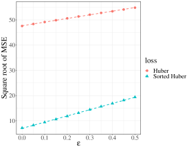
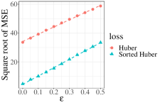
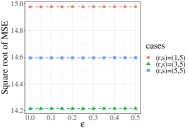
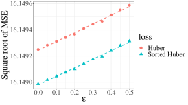
Let us illustrate considering the well-specified model with $\boldsymbol{\Gamma}^{*}\equiv\mathbf{0}$ and $q=2$. It is well known that, in linear regression, Huber’s estimator can be cast as a least-squares estimator in the augmented variable $[\boldsymbol{b},\boldsymbol{\theta}]$ with the penalization $\|\boldsymbol{\theta}\|_{1}$ [80, 39]. In this work, we penalize $\|\boldsymbol{\theta}\|_{\sharp}$ — i.e., we fit with the loss in Definition 1. Figure 1 plots the estimation error as a function of $\epsilon$ in sparse linear regression using synthetic contaminated data. We refer to Section 12 for details. We can see that the “Sorted” Huber loss significantly outperforms Huber regression. In this work, we present near-optimal bounds trying to explain this significant empirical observation. Roughly, the intuition is that the former loss assigns more weight to outliers with larger magnitude. Huber regression processes all label data points indistinguishably.

Figure 1: Huber vs “Sorted” Huber losses in sparse regression: $\sqrt{\texttt{MSE}}$ versus $\epsilon$.

4 Motivating examples

Matrix decomposition is motivated by several applications. We refer to [2] and Chapter 7 of the book [47] for a precise discussion and further references. They consider the general framework: to estimate the pair $[\mathbf{B}^{*},\boldsymbol{\Gamma}^{*}]\in(\mathds{R}^{p})^{2}$ given a noisy linear observation of its sum. Precisely, their model is $\mathbf{Y}=\mathfrak{X}(\mathbf{B}^{*}+\boldsymbol{\Gamma}^{*})+\boldsymbol{\Xi}$ where the design $\mathfrak{X}:\mathds{R}^{p}\rightarrow\mathbb{R}^{n\times m}$ takes values on matrices with $n$ iid rows and $\boldsymbol{\Xi}\in\mathbb{R}^{n\times m}$ is a noise matrix independent of $\mathfrak{X}$ with $n$ centered iid rows. It is further required that $\mathbf{B}^{*}$ is low-rank, $\boldsymbol{\Gamma}^{*}$ is a sparse matrix and that a “low-spikeness” conditions holds. Three subproblems are analyzed in the framework of [2]: factor analysis, robust covariance estimation and multi-task learning. The first two problems have identity designs ($\mathfrak{X}=I$). In multi-task learning, the design is invertible with high probability. Trace regression with additive matrix decomposition corresponds to their model with $m=1$ and design $\mathfrak{X}_{i}(\mathbf{B}):=\langle\mathchoice{{}\mkern-4.5mu}{{}\mkern-4.5mu}{{}\mkern-2.5mu}{}\langle\mathbf{X}_{i},\mathbf{B}\rangle\mathchoice{{}\mkern-4.5mu}{{}\mkern-4.5mu}{{}\mkern-2.5mu}{}\rangle$. Alternatively, it corresponds to (1) assuming the well-specified case, $\operatorname*{rank}(\mathbf{B}^{*})\leq r$ and $\|\boldsymbol{\Gamma}^{*}\|_{0}\leq s$ and $\boldsymbol{\theta}^{*}\equiv\mathbf{0}$. As discussed in item (d) of the introduction, the design property in [2] is not guaranteed to hold for this problem. More broadly, we consider additive matrix decomposition in trace regression when labels are contaminated.

To finish, we require the so called “low-spikeness” assumption: there exists $\mathsf{a}^{*}>0$ such that for any potential parameter $\mathbf{B}$, $\|\mathbf{B}\|_{\infty}\leq\nicefrac{{\mathsf{a}^{*}}}{{\sqrt{n}}}.$ For this problem, we consider estimator (7) with tuning $\mathsf{a}:=\mathsf{a}^{*}/\sqrt{n}$, $\mathcal{R}:=\|\cdot\|_{N}$ and $\mathcal{S}:=\|\cdot\|_{1}$. Two well known particular submodels of RTRMD are:

• Sparse regression [86, 10] is a particular case of model (3) with $d_{1}=p$, $d_{2}=1$, $\boldsymbol{x}:=\mathbf{X}\in\mathbb{R}^{p}$, $\boldsymbol{b}^{*}:=\mathbf{B}^{*}\in\mathbb{R}^{p}$, $\boldsymbol{\Gamma}^{*}\equiv\mathbf{0}$ and $\|\boldsymbol{b}^{*}\|_{0}\leq s\ll p$. In case of label contamination ($0\neq\|\boldsymbol{\theta}^{*}\|_{0}\leq o$), we consider estimators (9) with $q\in\{1,2\}$ and $\mathcal{R}:=\|\cdot\|_{1}$ or $\mathcal{R}=\|\cdot\|_{\sharp}$.

• Trace regression (or matrix sensing) [77, 76, 78, 68] correspond to model (3) with $\mathbf{B}^{*}\in\mathds{R}^{p}$ having rank $r\ll d_{1}\wedge d_{2}$ and $\boldsymbol{\Gamma}^{*}\equiv\mathbf{0}$. With contaminated labels, we consider estimators (9) with $q\in\{1,2\}$ and $\mathcal{R}:=\|\cdot\|_{N}$.

5 Results for RTRMD and robust sparse/low-rank regression

We state in this section optimal guarantees for the estimators (7)-(9) of models of Section 4. These are in fact particular consequences of our main results: Theorems 6-7, Proposition 2, Theorem 15 and Theorem 21. Being somewhat technical, we state them, respectively, in the later sections: Sections 7, 8, 10 and 11. As a prelude to the proofs in Sections 10-11, we include Section 9. It discusses the role of the multiplier process inequality (Theorem 6 in Section 7) within the framework of $M$-estimation with decomposable regularizers. Theorem 15, the main result of the paper, is a general deterministic result for estimator (7) and RTRMD. It assumes specific design properties presented in Definition 8 in Section 8. Proposition 2 in this section ensures these properties are satisfied with high probability. Its proof requires concentration inequalities stated in Theorems 6-7 of Section 7. Theorem 21 in Section 11 is a general deterministic result for estimator (9) with $q=1$ and the problem of robust trace regression (with no matrix decomposition). This theorem ensures this estimator is near-optimal adaptively to the noise variance. The proof of Theorem 21 is largely inspired by the proof of Theorem 15. These points are explained in detail later.

Next, we work with distributions satisfying the following assumption.

Assumption 2.

$\mathbf{X}$ is centered and $L$-subgaussian for some $L\geq 1$, that is, $|\langle\mathchoice{{}\mkern-4.5mu}{{}\mkern-4.5mu}{{}\mkern-2.5mu}{}\langle\mathbf{X},\mathbf{V}\rangle\mathchoice{{}\mkern-4.5mu}{{}\mkern-4.5mu}{{}\mkern-2.5mu}{}\rangle|_{\psi_{2}}\leq L\|\mathbf{V}\|_{\Pi}$ for all $\mathbf{V}\in\mathds{R}^{p}$. Additionally, $1\leq|\xi|_{\psi_{2}}=:\sigma<\infty$.

Define

$$\rho_{1}(\boldsymbol{\Sigma}):=\max_{j\in[p]}\boldsymbol{\Sigma}_{jj}^{1/2},\quad\mbox{ and }\quad\rho_{N}(\boldsymbol{\Sigma}):=\sup_{\|[\boldsymbol{z},\boldsymbol{v}]\|_{2}=1}\{\mathbb{E}(\boldsymbol{z}^{\top}\mathbf{X}\boldsymbol{v})^{2}\}^{1/2}.$$

Throughout the paper, we let $\boldsymbol{\Delta}^{\hat{\boldsymbol{\theta}}}:=\hat{\boldsymbol{\theta}}-\boldsymbol{\theta}^{*}$, $\boldsymbol{\Delta}_{\mathbf{B}}:=\widehat{\mathbf{B}}-\mathbf{B}$ and $\boldsymbol{\Delta}_{\boldsymbol{\Gamma}}:=\widehat{\boldsymbol{\Gamma}}-\boldsymbol{\Gamma},$ where $[\hat{\mathbf{B}},\hat{\boldsymbol{\Gamma}},\hat{\boldsymbol{\theta}}]$ denote estimators and $\mathbf{B},\boldsymbol{\Gamma}\in\mathds{R}^{p}$ are given points.

Next, we give guarantees for the estimator (7) and RTRMD. Given $r,s\in\mathbb{N}$ and $\mathsf{a}^{*},\mathsf{c}>0$, we define the class

$$\mathcal{F}(r,s,\mathsf{a}^{*},\mathsf{c}) :=\left\{[\mathbf{B},\boldsymbol{\Gamma}]\in(\mathds{R}^{p})^{2}:\begin{array}[]{c}\operatorname*{rank}(\mathbf{B})\leq r,\|\boldsymbol{\Gamma}\|_{0}\leq s,\\ (\nicefrac{{1}}{{n}})\|\mathfrak{X}(\mathbf{B}+\boldsymbol{\Gamma})-\boldsymbol{f}\|_{2}^{2}\leq\mathsf{c}\sigma^{2},\\ \|\mathbf{B}\|_{\infty}\leq\frac{\mathsf{a}^{*}}{\sqrt{n}}\end{array}\right\}.$$ (20)

Let $\omega(\epsilon):=\epsilon\log(1/\epsilon)$. Given $C_{1}>0$, define

$$r_{n,r,s,\delta}(\mathsf{a}^{*},C_{1}):=L\frac{1+\sqrt{\log(1/\delta)}}{\sqrt{n}}+L^{2}\left[\sqrt{\frac{r(d_{1}+d_{2})}{n}}+\sqrt{\frac{s\log p}{n}}\right]+\left(1+\frac{1}{C_{1}\sigma L}\right)\mathsf{a}^{*}\sqrt{\frac{s}{n}}.$$ (21)

Theorem 2 (Robust trace regression with additive matrix decomposition).

Grant Assumptions 1-2, model (1) and assume $\mathbf{X}$ is isotropic. Then there are absolute constants $\mathsf{c}\in(0,1)$, $c_{1}\in(0,1/2)$ and $C_{0},C_{1}\geq 1$ such that the following holds. Suppose $C_{1}^{2}L^{4}\epsilon\log(1/\epsilon)\leq c_{1}$. Given $\mathsf{a}^{*}>0$, let $[\hat{\mathbf{B}},\hat{\boldsymbol{\Gamma}}]$ be the solution of (7) with $\mathcal{R}:=\|\cdot\|_{N}$, $\mathcal{S}:=\|\cdot\|_{1}$ and with tuning parameters $\mathsf{a}:=\mathsf{a}^{*}/\sqrt{n}$, $\lambda\asymp\sigma L^{2}\sqrt{\nicefrac{{d_{1}+d_{2}}}{{n}}},$ $\chi\asymp\sigma L^{2}\sqrt{\nicefrac{{\log p}}{{n}}}+\nicefrac{{\mathsf{a}^{*}}}{{\sqrt{n}}}$ and $\tau\asymp C_{1}L^{2}\sigma/\sqrt{n}$. Assume that

$$n \gtrsim\left[L^{4}\cdot r(d_{1}+d_{2})\right]\bigvee\left[\left(L^{4}\log p+(\mathsf{a}^{*})^{2}\right)s\right].$$ (22)

Then, for any $\delta\in(0,1)$ such that $\delta\geq\exp\left(-\frac{n}{C_{0}L^{4}}\right),$ on an event of probability $\geq 1-\delta$, for all $[\mathbf{B},\boldsymbol{\Gamma}]\in\mathcal{F}(r,s,\mathsf{a}^{*},\mathsf{c})$,

$$(\nicefrac{{\lambda}}{{2}})\|\boldsymbol{\Delta}_{\mathbf{B}}\|_{N}+(\nicefrac{{\chi}}{{2}})\|\boldsymbol{\Delta}_{\boldsymbol{\Gamma}}\|_{1}+\|\mathfrak{X}^{(n)}(\hat{\mathbf{B}}+\hat{\boldsymbol{\Gamma}})-\boldsymbol{f}^{(n)}\|_{2}^{2} \leq\left(1+\frac{\mathcal{O}(1)}{C_{1}^{2}L^{2}}\right)\|\mathfrak{X}^{(n)}(\mathbf{B}+\boldsymbol{\Gamma})-\boldsymbol{f}^{(n)}\|_{2}^{2}$$ (23)

$$+\mathcal{O}(\sigma^{2})r_{n,r,s,\delta}^{2}(\mathsf{a}^{*},C_{1})+\mathcal{O}(C_{1}^{2}\sigma^{2}L^{6})\omega^{2}(\epsilon),$$ (24)

and also

$$\|[\boldsymbol{\Delta}_{\mathbf{B}},\boldsymbol{\Delta}_{\boldsymbol{\Gamma}}]\|_{\Pi} \leq\left(\mathcal{O}(1)+\frac{\mathcal{O}(1)}{C_{1}L}\right)\|\mathfrak{X}^{(n)}(\mathbf{B}+\boldsymbol{\Gamma})-\boldsymbol{f}^{(n)}\|_{2}+\mathcal{O}(\sigma)r_{n,r,s,\delta}(\mathsf{a}^{*},C_{1})+\mathcal{O}(C_{1}\sigma L^{3})\omega(\epsilon).$$ (25)

Theorem 2 states oracle inequalities of the form (2). The next proposition ensures the rate in Theorem 2 is optimal up to a log factor. Its proof follows from similar arguments in [2] for the noisy matrix decomposition problem with identity design. Define the class

$$\mathcal{A}(r,s,\mathsf{a}^{*})=\left\{\boldsymbol{\Theta}^{*}:=[\mathbf{B}^{*},\boldsymbol{\Gamma}^{*}]\in(\mathds{R}^{p})^{2}:\operatorname*{rank}(\mathbf{B}^{*})\leq r,\|\boldsymbol{\Gamma}^{*}\|_{0}\leq s,\|\mathbf{B}^{*}\|_{\infty}\leq\frac{\mathsf{a}^{*}}{\sqrt{n}}\right\}.$$ (26)

For any $\boldsymbol{\Theta}^{*}:=[\mathbf{B}^{*},\boldsymbol{\Gamma}^{*}]\in(\mathds{R}^{p})^{2}$, let $\mathbb{P}_{\boldsymbol{\Theta}^{*}}$ denote the distribution of the data $\{y_{i},\mathbf{X}_{i}\}_{i\in[n]}$ satisfying (3) with parameters $[\mathbf{B}^{*},\boldsymbol{\Gamma}^{*}]$. Finally, for some $\sigma>0$, let

$$\Psi_{n}(r,s,\mathsf{a}^{*}):=\sigma^{2}\left\{\frac{r(d_{1}+d_{2})}{n}+\frac{s}{n}\log\left(\frac{p-s}{s/2}\right)\right\}+(\mathsf{a}^{*})^{2}\frac{s}{n}.$$ (27)

Proposition 1.

Assume that $\{\xi_{i}\}_{i\in[n]}$ are iid $\mathcal{N}(0,\sigma^{2})$ independent of $\{\mathbf{X}_{i}\}_{i\in[n]}$, $\mathbf{X}$ is isotropic and $\|\mathbf{B}^{*}\|_{\infty}\leq\mathsf{a}^{*}/\sqrt{n}$. Assume $d_{1},d_{2}\geq 10$, $\mathsf{a}^{*}\geq 32\sqrt{\log p}$ and $s<p$.

Then there exists universal constants $c>0$ and $\beta\in(0,1)$ such that

$$\inf_{\hat{\boldsymbol{\Theta}}}\sup_{\boldsymbol{\Theta}^{*}\in\mathcal{A}(r,s,\mathsf{a}^{*})}\mathbb{P}_{\boldsymbol{\Theta}^{*}}\left\{\|[\boldsymbol{\Delta}_{\mathbf{B}^{*}},\boldsymbol{\Delta}_{\boldsymbol{\Gamma}^{*}}]\|_{\Pi}\geq c\Psi_{n}^{\frac{1}{2}}(r,s,\mathsf{a}^{*})\right\}\geq\beta,$$ (28)

where the infimum is taken over all estimators $\hat{\boldsymbol{\Theta}}=[\hat{\mathbf{B}},\hat{\boldsymbol{\Gamma}}]$ constructed from the data $\{y_{i},\mathbf{X}_{i}\}_{i\in[n]}$.

Next, we state guarantees for the estimator (9) with $q=2$ for three different parameter classes associated to the subproblems a)-b) in Section 4. Let $\|\cdot\|$ denote either $\|\cdot\|_{0}$ or the rank operation $\operatorname*{rank}(\cdot)$ and $\mathbb{C}_{\mathbf{B}}\subset\mathds{R}^{p}$ be a cone parametrized by a point $\mathbf{B}\in\mathds{R}^{p}$. Given $d,d_{\operatorname*{\tiny{eff}}}\in\mathbb{N}$ and $\rho,\mathsf{c},\mathsf{C}>0$, let $\mathcal{F}(d,d_{\operatorname*{\tiny{eff}}},\rho,\mathsf{C}):=\{\mathbf{B}\in\mathds{R}^{p}:\|\mathbf{B}\|\leq d,\mathsf{C}L^{2}\rho\mu\left(\mathbb{C}_{\mathbf{B}}\right)\sqrt{\nicefrac{{d_{\operatorname*{\tiny{eff}}}}}{{n}}}\leq 1\}$ and

$$\mathcal{F}(d,d_{\operatorname*{\tiny{eff}}},\rho,\mathsf{c},\mathsf{C}):=\left\{\mathbf{B}\in\mathcal{F}(d,d_{\operatorname*{\tiny{eff}}},\rho,\mathsf{C}):(\nicefrac{{1}}{{n}})\|\mathfrak{X}(\mathbf{B})-\boldsymbol{f}\|_{2}^{2}\leq\mathsf{c}\sigma^{2}\right\}.$$ (29)

Consider three cases:

• In sparse regression, take $\mathcal{R}:=\|\cdot\|_{1}$ and $\lambda\asymp L^{2}\sigma\rho_{1}(\boldsymbol{\Sigma})\sqrt{\nicefrac{{\log p}}{{n}}}.$ Set $\|\cdot\|:=\|\cdot\|_{0}$, $\rho:=\rho_{1}(\boldsymbol{\Sigma})$, $d:=s$, $d_{\operatorname*{\tiny{eff}}}:=s\log p$, and $\mathbb{C}_{\boldsymbol{b}}:=\mathcal{C}_{\boldsymbol{b},\|\cdot\|_{1}}(6)$ for given $\boldsymbol{b}$ — see Section 10 for the definition of this cone.

• In sparse regression, take $\mathcal{R}:=\|\cdot\|_{\sharp}$, the Slope norm in $\mathbb{R}^{p}$, and $\lambda\asymp L^{2}\sigma\rho_{1}(\boldsymbol{\Sigma})/\sqrt{n}.$ Set $\|\cdot\|:=\|\cdot\|_{0}$, $\rho:=\rho_{1}(\boldsymbol{\Sigma})$, $d:=s$, $d_{\operatorname*{\tiny{eff}}}:=s\log(ep/s)$, and the cone $\mathbb{C}_{\boldsymbol{b}}:=\overline{\mathcal{C}}_{s}(6)$ for each $\boldsymbol{b}$ such that $\|\boldsymbol{b}\|_{0}\leq s$ — see Section 31

• In trace regression, take $\mathcal{R}:=\|\cdot\|_{N}$ and $\lambda\asymp L^{2}\sigma\rho_{N}(\boldsymbol{\Sigma})\sqrt{\nicefrac{{d_{1}+d_{2}}}{{n}}}.$ Set $\|\cdot\|:=\operatorname*{rank}(\cdot)$, $\rho:=\rho_{N}(\boldsymbol{\Sigma})$, $d:=r$, $d_{\operatorname*{\tiny{eff}}}:=r(d_{1}+d_{2})$ and the cone $\mathbb{C}_{\mathbf{B}}:=\mathcal{C}_{\mathbf{B},\|\cdot\|_{N}}(6)$ for given $\mathbf{B}$ — see Section 10.

Let us define

$$r_{n,d_{\operatorname*{\tiny{eff}}},\delta}(\rho,\mu):=L\frac{1+\sqrt{\log(1/\delta)}}{\sqrt{n}}+L^{2}\rho\mu\sqrt{\frac{d_{\operatorname*{\tiny{eff}}}}{n}}.$$ (30)

Theorem 3 (Robust sparse/low-rank regression).

Grant Assumptions 1-2 and model (1). Then there are absolute constants $\mathsf{c},c_{1}\in(0,1/2)$ and $\mathsf{C},C_{0},C_{1}\geq 1$ such that the following holds. Suppose $C_{1}^{2}L^{4}\epsilon\log(1/\epsilon)\leq c_{1}$ and take $\tau\asymp C_{1}L^{2}\sigma/\sqrt{n}$. Let $\hat{\mathbf{B}}$ be the solution of (9) with $q=2$ — correspondingly to each tuning in cases (i)-(iii). Consider the three different classes of type (29) for each of the cases (i)-(iii).

Then, for any $\delta\in(0,1)$ such that $\delta\geq\exp\left(-\frac{n}{C_{0}L^{4}}\right),$ on an event of probability $\geq 1-\delta$, for all $\mathbf{B}\in\mathcal{F}(d,d_{\operatorname*{\tiny{eff}}},\rho,\mathsf{c},\mathsf{C})$,

$$(\nicefrac{{\lambda}}{{2}})\mathcal{R}(\boldsymbol{\Delta}_{\mathbf{B}})+\|\mathfrak{X}^{(n)}(\hat{\mathbf{B}})-\boldsymbol{f}^{(n)}\|_{2}^{2} \leq\left(1+\frac{\mathcal{O}(1)}{C_{1}^{2}L^{2}}\right)\|\mathfrak{X}^{(n)}(\mathbf{B})-\boldsymbol{f}^{(n)}\|_{2}^{2}$$ (31)

$$+\mathcal{O}(\sigma^{2})r_{n,d_{\operatorname*{\tiny{eff}}},\delta}^{2}(\rho,\mu(\mathbb{C}_{\mathbf{B}}))+\mathcal{O}(C_{1}^{2}\sigma^{2}L^{6})\omega^{2}(\epsilon),$$ (32)

and also

$$\|\boldsymbol{\Delta}_{\mathbf{B}}\|_{\Pi} \leq\left(\mathcal{O}(1)+\frac{\mathcal{O}(1)}{C_{1}L}\right)\|\mathfrak{X}^{(n)}(\mathbf{B})-\boldsymbol{f}^{(n)}\|_{2}+\mathcal{O}(\sigma)r_{n,d_{\operatorname*{\tiny{eff}}},\delta}(\rho,\mu(\mathbb{C}_{\mathbf{B}}))+\mathcal{O}(C_{1}\sigma L^{3})\omega(\epsilon).$$ (33)

From the quadratic process inequality, we may replace $\rho_{1}(\boldsymbol{\Sigma})$ with $\hat{\rho}_{1}:=\max_{j\in[p]}\|\mathbb{X}_{\bullet,j}\|_{2}$ and $\rho_{N}(\boldsymbol{\Sigma})$ by its empirical counterpart $\hat{\rho}_{N}$. We now present estimation guarantees for the estimator (9) with $q=1$. Consider three cases:

• Grant case (i) above but with $\lambda\asymp L\rho_{1}(\boldsymbol{\Sigma})\sqrt{\nicefrac{{\log p}}{{n}}}.$

• Grant case (ii) above but with $\lambda\asymp L\rho_{1}(\boldsymbol{\Sigma})/\sqrt{n}.$

• Grant case (iii) above but with $\lambda\asymp L\rho_{N}(\boldsymbol{\Sigma})\sqrt{\nicefrac{{d_{1}+d_{2}}}{{n}}}.$

Theorem 4 ($\sigma$-adaptive robust sparse/low-rank regression).

Grant Assumptions 1-2 and model (1). Then there are absolute constants $c_{1}\in(0,1/2)$ and $\mathsf{C},C_{0}\geq 1$ such that the following holds. Suppose $L^{2}\epsilon\log(1/\epsilon)\leq c_{1}$ and take $\tau\asymp L/\sqrt{n}$. Let $\hat{\mathbf{B}}$ be the solution of (9) with $q=1$ — correspondingly to each tuning in cases (i’)-(iii’). Consider the three different classes of type (29) for each of the cases (i’)-(iii’).

Let $\delta\in(0,1)$ such that $\delta\geq\exp\left(-\frac{n}{C_{0}(L^{4}\vee\sigma^{2})}\right).$ Let $\mu_{*}:=\sup_{\mathbf{B}\in\mathcal{F}(d,d_{\operatorname*{\tiny{eff}}},\rho,\mathsf{C})}\mu(\mathbb{C}_{\mathbf{B}})$ and $\mathsf{c}_{0,n}\asymp r_{n,d_{\operatorname*{\tiny{eff}}},\delta}(\rho,\mu_{*})$. Then, on an event of probability $\geq 1-\delta$, it holds that, for all $\mathbf{B}\in\mathcal{F}(d,d_{\operatorname*{\tiny{eff}}},\rho,\mathsf{c}_{0,n}^{2},\mathsf{C})$,

$$(\nicefrac{{\lambda}}{{2}})\mathcal{R}(\boldsymbol{\Delta}_{\mathbf{B}})+\|\mathfrak{X}^{(n)}(\hat{\mathbf{B}})-\boldsymbol{f}^{(n)}\|_{2}^{2} \leq\left(1+\mathcal{O}(\mathsf{c}_{0,n}^{2})\right)\|\mathfrak{X}^{(n)}(\mathbf{B})-\boldsymbol{f}^{(n)}\|_{2}^{2}$$ (34)

$$+\mathcal{O}(\sigma^{2})r_{n,d_{\operatorname*{\tiny{eff}}},\delta}^{2}(\rho,\mu_{*})+\mathcal{O}(\sigma^{2}L^{4})\omega^{2}(\epsilon),$$ (35)

and also

$$\|\boldsymbol{\Delta}_{\mathbf{B}}\|_{\Pi} \leq\left(\mathcal{O}(1)+\mathcal{O}(\mathsf{c}_{0,n})\right)\|\mathfrak{X}^{(n)}(\mathbf{B})-\boldsymbol{f}^{(n)}\|_{2}+\mathcal{O}(\sigma)r_{n,d_{\operatorname*{\tiny{eff}}},\delta}(\rho,\mu_{*})+\mathcal{O}(\sigma L^{2})\omega(\epsilon).$$ (36)

In all previous theorems, the correspondent estimator is adaptive to $\delta$ and the confidence level is $1-\delta$ across any $\delta\geq\exp(-cn)$ for a fixed constant $c>0$. The estimators are also adaptive to $(s,r,o)$, and, in Theorems 3-4, adaptive to $\mu(\mathbb{C}_{\mathbf{B}})$. In case there is no matrix decomposition, estimator (9) with $q=1$ achieves, up to constants, the same rate of estimator (9) with $q=2$ with the advantage of being adaptive to $\sigma$. On the other hand, for $q=1$ the approximation must be $\mathcal{O}(\sigma)r_{n,d_{\operatorname*{\tiny{eff}}},\delta}(\rho,\mu_{*})$ while for $q=2$ the approximation error is only required to be $\mathcal{O}(\sigma)$. Nothing is assumed beyond marginal subgaussianity of $(\mathbf{X},\xi)$. In particular, the noise can depend arbitrarily on $\mathbf{X}$, be asymmetric and have zero mass around the origin. From [15], the displayed rates are optimal up to the factor $\log(1/\epsilon)$. The approximately linear growth $\epsilon\mapsto\omega(\epsilon)$ — in case the sorted Huber loss is used — is confirmed in our numerical experiments (see Section 12).

Remark 2.

Within the framework of $M$-estimation with decomposable regularizers, the first obtained oracle inequalities for sparse and trace regression give optimal rates in average [10, 69]. Still, as discussed in Section 9, the rates in these seminal works are suboptimal in $\delta$. Additionally, their tuning assumes knowledge of $\delta$. [6] was the first work to obtain the subgaussian rate with $\delta$-adaptive estimators for sparse linear regression. [31] later generalized the bounds of [6] for the square-root Lasso estimator. Their proof strategy, however, fundamentally assumes the noise is independent of features (see Section 9). When $\epsilon=0$, a corollary of Theorems 3-4 is that the same estimators in [6, 31] attain the subgaussian rate adaptively to $\delta$ assuming only $(\mathbf{X},\xi)$ are marginally subgaussian. We refer to Section 9 and Remark 6 in Section 7 for an explanation on these technical issues. See also Section 6.3. To finish, we remark that when $\epsilon=0$ we could prove “sharp” oracle inequalities — that is, with constant $C=1$ in (2).

6 Related work and contributions

6.1 Robust sparse regression

This model has been the subject of numerous works. From a methodological point of view, the $\ell_{1}$-penalized Huber’s estimator has been considered in [79, 80, 58]. Empirical evaluation for the choice of tuning parameters is comprehensively studied in these papers. For the adversarial model with Gaussian data, fast rates for such estimator have been obtained in [12, 56, 26, 25, 71]. The average near optimal rate was shown only recently in [27]. They obtain the rate $\sqrt{s\log(p/\delta)/n}+\epsilon\log(n/\delta),$ with a breakdown point $\epsilon\leq c/\log n$ for a constant $c>0$. Under different conditions, the same estimator was later shown in [24] to attain the subgaussian rate with breakdown point $\epsilon\leq c$ without the extra factor $\log(1/\epsilon)$ and allowing feature-dependent heavy-tailed noise. These two works are the most closely related to our particular Theorem 3 for robust sparse linear regression.

Remark 3 (Comparison with [24]).

The result in [24] is interesting: the subgaussian rate is attainable with the standard Huber loss — without the extra $\log(1/\epsilon)$. It also allows feature-dependent heavy-tailed noise — assuming some extra mild conditions. Still, we argue that, in the subgaussian setting, this result is weaker than our Theorem 3 for a sparse parameter. We give two main reasons:

• Even though not explicitly stated, the proof in [24] is specific to the oblivious model — a much weaker model than the adversarial one considered in this work. If $\mathcal{O}$ denotes the index set of outliers, they fundamentally use that, for all $[\boldsymbol{b},\boldsymbol{b}^{\prime}]$,

  $$\left|\frac{1}{o}\sum_{i\in\mathcal{O}}(|\langle\boldsymbol{x}_{i},\boldsymbol{b}-\boldsymbol{b}^{\prime}\rangle|-\mathbb{E}[|\langle\boldsymbol{x},\boldsymbol{b}-\boldsymbol{b}^{\prime}\rangle|])\right|_{\psi_{2}}\lesssim\frac{\|\boldsymbol{b}-\boldsymbol{b}^{\prime}\|_{\Pi}}{\sqrt{o}}.$$ (37)

  This follows from Hoeffding’s inequality, but only if $\{\boldsymbol{x}_{i}\}_{i\in\mathcal{O}}$ is iid for fixed $\mathcal{O}$. In the adversarial model, $\mathcal{O}$ is an arbitrary random variable dependent on the data set.

• [24] attains the optimal rate for $\ell_{1}$-regularized Huber regression with penalization

  $$\lambda\asymp\sigma\left(\sqrt{\frac{\log p}{n}}\bigvee\mu(\mathbb{C}_{\boldsymbol{b}^{*}})\sqrt{\frac{\log(1/\delta)}{sn}}\bigvee\mu(\mathbb{C}_{\boldsymbol{b}^{*}})\frac{o}{\sqrt{s}n}\right),$$ (38)

  and, in case the noise is subgaussian, $\tau\asymp\sigma$. Our tuning $(\lambda,\tau)$ follows the very different scaling $\lambda\asymp\sigma\sqrt{\log p/n},$ $\tau\asymp\sigma/\sqrt{n}.$ One notable difference is that our tuning is adaptive to $(s,o,\mu(\mathbb{C}_{\boldsymbol{b}^{*}}),\delta)$, without resorting to Lepski’s method. If we focus on $(s,o,\mu(\mathbb{C}_{\boldsymbol{b}^{*}}),\delta)$-adaptive estimators, our guarantees and simulation results are significantly in favor of sorted Huber-type losses instead of the standard Huber loss.

We argue that (i) and the different scaling (38) follows from a different proof method. The proof in [24] is based on “localization” arguments for regularized empirical risk minimization (ERM) [64, 57]. Being more precise, [24] is able to show that regularized ERM with convex Lipschitz losses [3, 23] is robust against contaminated labels, assuming the oblivious model. In this approach, one uses the fact that the loss based on Huber’s function satisfies the so called “Bernstein’s condition” — under additional mild noise conditions. Our proof method does not follow the “localization” literature but rather the literature on $M$-estimation with decomposable regularizers [10, 69, 6]. In this approach, we do not use Lipschitz continuity of Huber-type losses. In fact, our analysis uses a loss based on the square cost and defined over an augmented variable — see (12)-(14).

Remark 4 (Comparison with [27]).

Granting reasons (i)-(ii) in Remark 3, [27] is the closest work to ours — indeed, they consider the adversarial model and $(s,o,\mu(\mathbb{C}_{\boldsymbol{b}^{*}}))$-adaptive estimators. Our most noted improvements in terms of rate guarantees are three-fold. First, we show that sorted Huber-type regression has improved bounds compared to Huber-regression: the corruption error $\epsilon\log n$ and breakdown point $c/\log n$ of the latter is replaced by $\epsilon\log(1/\epsilon)$ and breakdown point $c$. We give numerical evidence of the superiority of sorted Huber regression compared to standard Huber regression (see Figure 1). Adaptations of Huber regression have been studied before. Still, they usually involve modifying the scaling of the tuning parameter. To our knowledge, our theoretical and empirical results for sorted Huber-type losses give new insights. Second, unlike the results in [27], our rates for sparse regression use $\delta$-adaptive estimators attaining the optimal $\delta$-subgaussian rate under weaker assumptions — namely, subgaussian feature-dependent noise. See Remark 2, Section 6.3 and pointers therein. Thirdly, we give optimal guarantees for robust sparse regression with $\sigma$-adaptive estimators under the same set of assumptions. In Section 11, we explain that the proof of Theorem 4 is an adaptation of the proof of Theorem 3.

To finish, we remark that our improvements on [27] are substantial in terms of proof techniques and structural properties. In fact, our main focus is the broader model RTRMD. See the next Section 6.3 and pointers therein.

Remark 5 (Further references in robust sparse regression).

We complement our review mentioning some literature analyzing different contamination models, e.g. dense bounded noise [88, 59, 70, 42, 1]. This setting is also studied in [51] with the LAD-estimator [87]. Alternatively, a refined analysis of iterative thresholding methods were considered in [9, 8, 82, 67]. They obtain sharp breakdown points and consistency bounds for the oblivious model. Works on sparse linear regression with covariate contamination were considered early on by [18] and, more recently, in [4], albeit with worst rates and breakdown points compared to the response contamination model. Works by [60, 61] have also studied the optimality of sparse linear regression in models with error-in-variables and missing-data covariates. Although out of scope, we mention for completeness that tractable algorithms for linear regression with covariate contamination have been intensively investigated in the low-dimensional scaling ($n\geq p$), with initial works by [34, 36, 75] and more recent ones in [29, 22, 73, 72].

6.2 Robust trace regression

The first bounds on trace regression (with no corruption) were presented, e.g., in [68, 78, 69, 90] following the framework of $M$-estimation with decomposable regularizers. Trace regression with label-feature contamination is studied in detail in [44]. This paper is based on Tukey’s depth, a hard computational problem in high dimensions. The recent papers [41, 81] focus on models with heavy-tailed noise. The interesting paper [81] considers label contamination as well, but follows a methodology based on non-convex optimization, presenting bounds for a gradient-descent method. As such, it is hard to compare their results with ours, as they follow different set of assumptions. For instance, they assume the oblivious model — a more restrictive model than the adversarial one. Other minor differences include the assumptions that the covariance matrix is invertible, the noise has positive density around the origin and that some conditions are satisfied to ensure good initialization.

Robust trace regression is not considered in [24, 27]. Still, their methods could be applied to this problem. In that case, the exact same comments in Remarks 3-4 would still apply — changing $(s,\log p)$ by $(r,d_{1}+d_{2})$. As mentioned in Section 6.1, our improvements on guarantees and assumptions are in fact consequences of new proof techniques and structural design properties motivated to study the broader model RTRMD. We discuss this point in the next section.

6.3 Robust trace regression with additive matrix decomposition

The statistical theory for this model is the main concern of this work. In fact, the results in Sections 6.1-6.2 are consequences of the techniques needed to analyze the broader model RTRMD. As mentioned in the introduction, additive matrix decomposition was extensively studied in [89, 14, 13, 91, 48, 63, 2]. Still, there is currently no optimality theory for additive matrix decomposition in trace regression — nor its extension with label contamination. In this preliminary section, we briefly comment on three design properties needed to establish an optimality theory for RTRMD. A detailed discussion is referred to later sections.

When the parameter is the sum of a low-rank and sparse matrices, the random design in trace regression is singular with high probability. We identify a concentration inequality for the product process (see our Theorem 7) as the sufficient property to prove restricted strong convexity for this model. In Definition 8 in Section 8, we denote this property by $\operatorname*{PP}$. To the best of our knowledge, this is a novel application of product processes in high-dimensional statistics. This technical property is “sharp”, in the sense that replacing it with other naive methods, e.g. dual-norm inequalities, fail to entail the optimal rate.

$\operatorname*{PP}$ is no longer sufficient in case of label contamination. To handle it, we take inspiration from [27]. This work identified one design property sufficient to handle label contamination when the parameter is sparse. Termed “incoherence principle” ($\operatorname*{IP}$), it is derived from Chevet’s inequality. [27] is not concerned with matrix decomposition, and as such, $\operatorname*{PP}$ is unnecessary. We show that a generalized version of $\operatorname*{IP}$ (see Definition 8 in Section 8) and the new property $\operatorname*{PP}$ are jointly sufficient properties to ensure restricted strong convexity for RTRMD and to optimaly control the “design-corruption interaction”. Again, $\operatorname*{PP}$ and $\operatorname*{IP}$ are “sharp”: mere use of dual-norm inequalities fail to achieve optimality. See Remarks 7-8 in Section 8 and Remarks 9-11 in Section 10.

The third design property we use enables us to achieve the optimal $\delta$-subgaussian rate with $\delta$-adaptive estimators, even when the noise is feature-dependent. This property, denoted by $\operatorname*{MP}$ in Definition 8 in Section 8, follows from a concentration inequality for the multiplier process (see Theorem 6 in Section 7). In the framework of $M$-estimation with decomposable regularizers, $\operatorname*{MP}$ is a classical property used to control the “design-noise interaction” [10, 2, 6, 27]. The typical way to prove it is via the dual-norm inequality [10, 2, 27]. This approach fails to entail the subgaussian rate and $\delta$-adaptivity. [6] was the first to succeed on this point, using a suitable version of $\operatorname*{MP}$ (see Remark 2). Still, they assume feature-independent noise — in case the parameter is sparse and there is no contamination. Our version of $\operatorname*{MP}$ in Definition 8 in Section 8 is more general than [6] so to handle feature-dependent noise, additive matrix decomposition and label contamination.

To finish, as discussed in Section 6.1, the relevance of sorted Huber-type losses also applies to RTRMD. Using the standard Huber’s loss, we would have rate $\omega(\epsilon)\asymp\epsilon\log n$ instead of $\omega(\epsilon)\asymp\epsilon\log(1/\epsilon)$, breakdown point $\epsilon\leq c/\log n$ instead of $c$, for some constant $c\in(0,1/2)$. See also Figure 5(b) in Section 12.

7 The multiplier and product processes

In this section we present concentration inequalities for subgaussian Multiplier and Product processes with optimal dependence on $(d_{\operatorname*{\tiny{eff}}},\delta)$. The notation in this section is independent of all previous sections. Throughout this section, $(B,\mathcal{B},\mathbf{P})$ is a probability space, $(\xi,X)$ is a random (possibly not independent) pair taking values on $\mathbb{R}\times B$ and $X$ has marginal distribution $\mathbf{P}$. $\{(\xi_{i},X_{i})\}_{i\in[n]}$ will denote an iid copy of $(\xi,X)$ and $\hat{\mathbf{P}}$ be denotes the empirical measure associated to $\{X_{i}\}_{i\in[n]}$. The multiplier process over functions $f\in F$ is defined as

$$M(f):=\frac{1}{n}\sum_{i\in[n]}(\xi_{i}f(X_{i})-\mathbb{E}[\xi f(X)]).$$

For instance, the empirical process is a particular case when $\xi\equiv 1$. The product process is defined as

$$A(f,g):=\frac{1}{n}\sum_{i\in[n]}\bigg{\{}f(X_{i})g(X_{i})-\mathbb{E}f(X_{i})g(X_{i})\bigg{\}},$$

over two distinct classes $F$ and $G$ of measurable functions. When $F=G$, the correspondent process is often termed the quadratic process.

There is a large literature on concentration of these processes and its use in risk minimization. One pioneering idea is of “generic chaining”, first developed by Talagrand for the empirical process [83]. This method was refined by Dirksen, Bednorz, Mendelson and collaborators, e.g., in [66, 37, 5, 65]. The following notion of complexity is used in generic chaining bounds.

Definition 5 ($\gamma_{2,p}$-functional).

Let $(T,\mathsf{d})$ be a pseudo-metric space. We say a sequence $(T_{k})$ of subsets of $T$ is admissible if $|T_{0}|=1$ and $|T_{k}|\leq 2^{2^{k}}$ for $k\in\mathbb{N}$ and $\cup_{k\geq 0}T_{k}$ is dense in $T$. Let $\mathcal{A}$ denote the class of all such admissible subset sequences. Given $p\geq 1$, the $\gamma_{2,p}$-functional with respect to $(T,\mathsf{d})$ is the quantity

$$\gamma_{2,p}(T):=\inf_{(T_{k})\in\mathcal{A}}\sup_{t\in T}\sum_{k\geq\lfloor\log_{2}p\rfloor}2^{k/2}\mathsf{d}(t,T_{k}).$$ (39)

We will say that $(T_{k})\in\mathcal{A}$ is optimal if it achieves the infimum above. Set $\gamma_{2}(T):=\gamma_{2,1}(T)$.

Let $L_{\psi_{2}}=L_{\psi_{2}}(\mathbf{P})$ be the family of measurable functions $f:B\rightarrow\mathbb{R}$ having finite $\psi_{2}$-norm

$$\|f\|_{\psi_{2}}:=|f(X)|_{\psi_{2}}:=\inf\{c>0:\mathbb{E}[\psi_{2}(\nicefrac{{f(X)}}{{c}})]\leq 1\}$$

where $\psi_{2}(t):=e^{t^{2}}-1$. We assume that the $\psi_{2}$-norm of $\xi$, denoted also by $\|\xi\|_{\psi_{2}}$, is finite. Given $f,g\in L_{\psi_{2}}$, we define the pseudo-distance $\mathsf{d}(f,g):=\|f-g\|_{\psi_{2}}.$ Given a subclass $F\subset L_{\psi_{2}}$, we let $\Delta(F):=\sup_{f,f^{\prime}\in F}\mathsf{d}(f,f^{\prime})$ and $\bar{\Delta}(F):=\sup_{f\in F}\mathsf{d}(f,0)$. We prove the following two results in Sections B and C

Theorem 6 (Multiplier process).

There exists universal constant $c>0$, such that for all $f_{0}\in F$, $n\geq 1$, $u\geq 1$ and $v\geq 1$, with probability at least $1-ce^{-u/4}-ce^{-nv}$,

$$\sup_{f\in F}|M(f)-M(f_{0})| \lesssim\left(\sqrt{v}+1\right)\|\xi\|_{\psi_{2}}\frac{\gamma_{2}(F)}{\sqrt{n}}+\left(\sqrt{\frac{2u}{n}}+\frac{u}{n}+\sqrt{\frac{uv}{n}}\right)\|\xi\|_{\psi_{2}}\bar{\Delta}(F).$$ (40)

Theorem 7 (Product process).

Let $F,G$ be subclasses of $L_{\psi_{2}}$. There exist universal constants $c,C>0$, such that for all $n\geq 1$ and $u\geq 1$, with probability at least $1-e^{-u}$,

$$\sup_{(f,g)\in F\times G}\left|A(f,g)\right| \leq C\left[\frac{\gamma_{2}(F)\gamma_{2}(G)}{n}+\bar{\Delta}(F)\frac{\gamma_{2}(G)}{\sqrt{n}}+\bar{\Delta}(G)\frac{\gamma_{2}(F)}{\sqrt{n}}\right]$$ (41)

$$+c\sup_{(f,g)\in F\times G}\|fg-\mathbf{P}fg\|_{\psi_{1}}\left(\sqrt{\frac{u}{n}}+\frac{u}{n}\right).$$ (42)

Remark 6 (Confidence level & complexity).

Mendelson [65] established impressive concentration inequalities for the multiplier and product processes. In fact, they hold for much more general $(\xi,X)$ having heavier tails (see Theorems 1.9, 1.13 and 4.4 in [65]). When specifying these bounds to subgaussian classes and noise, however, the confidence parameter $u>0$ multiplies the complexities $\gamma_{2}(F)$ and $\gamma_{2}(G)$ — unlike our Theorems 6-7. For a related discussion regarding the empirical and quadratic processes, we refer to Remark 3.3(ii) and observations before Corollary 5.7 in Dirksen’s paper [37]. This technical point is crucial in our proof to show that our class of estimators attain the $\delta$-subgaussian rate in the high-dimensional regime with $\delta$-adaptive estimators. We refer to Section 9 for a discussion on this topic. Note that we can take $v\asymp 1$ for failure probability $\delta\geq e^{-c^{\prime}n}$ for absolute constant $c^{\prime}>0$. Our proofs are motivated by Dirksen’s method for the quadratic process [37] and Talagrand’s proof for the empirical process [83].

8 Properties for subgaussian distributions

In what follows, $\mathfrak{M}(\mathbf{V},\boldsymbol{u}):=\mathfrak{X}(\mathbf{V})+\sqrt{n}\boldsymbol{u},$ $\mathcal{R}$ and $\mathcal{S}$ are norms on $\mathds{R}^{p}$ and $\mathcal{Q}$ is a norm on $\mathbb{R}^{n}$. Throughout this section, $(\mathbf{X},\xi)\in\mathds{R}^{p}\times\mathbb{R}$ satisfies Assumption 2. Next, we define the empirical bilinear form

$$\langle\mathchoice{{}\mkern-4.5mu}{{}\mkern-4.5mu}{{}\mkern-2.5mu}{}\langle\mathbf{V},\mathbf{W}\rangle\mathchoice{{}\mkern-4.5mu}{{}\mkern-4.5mu}{{}\mkern-2.5mu}{}\rangle_{n}:=\frac{1}{n}\sum_{i\in[n]}\langle\mathchoice{{}\mkern-4.5mu}{{}\mkern-4.5mu}{{}\mkern-2.5mu}{}\langle\mathbf{X}_{i},\mathbf{V}\rangle\mathchoice{{}\mkern-4.5mu}{{}\mkern-4.5mu}{{}\mkern-2.5mu}{}\rangle\langle\mathchoice{{}\mkern-4.5mu}{{}\mkern-4.5mu}{{}\mkern-2.5mu}{}\langle\mathbf{X}_{i},\mathbf{W}\rangle\mathchoice{{}\mkern-4.5mu}{{}\mkern-4.5mu}{{}\mkern-2.5mu}{}\rangle=\langle\mathfrak{X}^{(n)}(\mathbf{V}),\mathfrak{X}^{(n)}(\mathbf{W})\rangle.$$

In what follows, $\{\mathsf{a}_{i},\mathsf{b}_{i},\mathsf{c}_{i},\mathsf{d}_{i},\mathsf{f}_{i}\}$ are fixed positive numbers.

Definition 8.

• $\mathfrak{X}$ satisfies $\operatorname*{RSC}_{\mathcal{R}}(\mathsf{a}_{1},\mathsf{a}_{2})$ if for all $\mathbf{V}\in\mathds{R}^{p}$,

  $$\big{\|}\mathfrak{X}^{(n)}(\mathbf{V})\big{\|}_{2}\geq\mathsf{a}_{1}\|\mathbf{V}\|_{\Pi}-\mathsf{a}_{2}\mathcal{R}(\mathbf{V}).$$ (43)

• $\mathfrak{X}$ satisfies $\operatorname*{PP}_{\mathcal{R},\mathcal{S}}(\mathsf{c}_{1},\mathsf{c}_{2},\mathsf{c}_{3},\mathsf{c}_{4})$ if for all $[\mathbf{V},\mathbf{W}]\in(\mathds{R}^{p})^{2}$,

  $$\left|\langle\mathchoice{{}\mkern-4.5mu}{{}\mkern-4.5mu}{{}\mkern-2.5mu}{}\langle\mathbf{V},\mathbf{W}\rangle\mathchoice{{}\mkern-4.5mu}{{}\mkern-4.5mu}{{}\mkern-2.5mu}{}\rangle_{n}-\langle\mathchoice{{}\mkern-4.5mu}{{}\mkern-4.5mu}{{}\mkern-2.5mu}{}\langle\mathbf{V},\mathbf{W}\rangle\mathchoice{{}\mkern-4.5mu}{{}\mkern-4.5mu}{{}\mkern-2.5mu}{}\rangle_{\Pi}\right| \leq\mathsf{c}_{1}\left\|\mathbf{V}\right\|_{\Pi}\|\mathbf{W}\|_{\Pi}+\mathsf{c}_{2}\mathcal{R}(\mathbf{V})\|\mathbf{W}\|_{\Pi}+\mathsf{c}_{3}\left\|\mathbf{V}\right\|_{\Pi}\mathcal{S}(\mathbf{W})$$ (44)

  $$\quad+\mathsf{c}_{4}\mathcal{R}(\mathbf{V})\mathcal{S}(\mathbf{W}).$$ (45)

• $\mathfrak{X}$ satisfies $\operatorname*{IP}_{\mathcal{R},\mathcal{S},\mathcal{Q}}(\mathsf{b}_{1},\mathsf{b}_{2},\mathsf{b}_{3},\mathsf{b}_{4})$ if for all $[\mathbf{V},\mathbf{W},\boldsymbol{u}]\in(\mathds{R}^{p})^{2}\times\mathbb{R}^{n}$,

  $$|\langle\boldsymbol{u},\mathfrak{X}^{(n)}(\mathbf{V}+\mathbf{W})\rangle| \leq\mathsf{b}_{1}\left\|[\mathbf{V},\mathbf{W}]\right\|_{\Pi}\|\boldsymbol{u}\|_{2}+\mathsf{b}_{2}\mathcal{R}(\mathbf{V})\|\boldsymbol{u}\|_{2}+\mathsf{b}_{3}\mathcal{S}(\mathbf{W})\|\boldsymbol{u}\|_{2}$$ (46)

  $$+\mathsf{b}_{4}\left\|[\mathbf{V},\mathbf{W}]\right\|_{\Pi}\mathcal{Q}(\boldsymbol{u}).$$ (47)

• $\mathfrak{X}$ satisfies $\operatorname*{ARSC}_{\mathcal{R},\mathcal{S},\mathcal{Q}}(\mathsf{d}_{1},\mathsf{d}_{2},\mathsf{d}_{3},\mathsf{d}_{4})$ if for all $[\mathbf{V},\mathbf{W},\boldsymbol{u}]\in(\mathds{R}^{p})^{2}\times\mathbb{R}^{n}$,

  $$\left\{\|\mathfrak{M}^{(n)}(\mathbf{V}+\mathbf{W},\boldsymbol{u})\|_{2}^{2}-2\langle\mathchoice{{}\mkern-4.5mu}{{}\mkern-4.5mu}{{}\mkern-2.5mu}{}\langle\mathbf{V},\mathbf{W}\rangle\mathchoice{{}\mkern-4.5mu}{{}\mkern-4.5mu}{{}\mkern-2.5mu}{}\rangle_{\Pi}\right\}_{+}^{\frac{1}{2}} \geq\mathsf{d}_{1}\|[\mathbf{V},\mathbf{W},\boldsymbol{u}]\|_{\Pi}-\mathsf{d}_{2}\mathcal{R}(\mathbf{V})-\mathsf{d}_{3}\mathcal{S}(\mathbf{W})-\mathsf{d}_{4}\mathcal{Q}(\boldsymbol{u}).$$ (48)

• $(\mathfrak{X},\boldsymbol{\xi})$ satisfies $\operatorname*{MP}_{\mathcal{R},\mathcal{S},\mathcal{Q}}(\mathsf{f}_{1},\mathsf{f}_{2},\mathsf{f}_{3},\mathsf{f}_{4})$ if for all $[\mathbf{V},\mathbf{W},\boldsymbol{u}]\in(\mathds{R}^{p})^{2}\times\mathbb{R}^{n}$,

  $$|\langle\boldsymbol{\xi}^{(n)},\mathfrak{M}^{(n)}(\mathbf{V}+\mathbf{W},\boldsymbol{u})\rangle|\leq\mathsf{f}_{1}\|[\mathbf{V},\mathbf{W},\boldsymbol{u}]\|_{\Pi}+\mathsf{f}_{2}\mathcal{R}(\mathbf{V})+\mathsf{f}_{3}\mathcal{S}(\mathbf{W})+\mathsf{f}_{4}\mathcal{Q}(\boldsymbol{u}).$$ (49)

In the next lemmas, we show that $\operatorname*{RSC}$ and $\operatorname*{ARSC}$ are consequences of $\operatorname*{PP}$ and $\operatorname*{IP}$.

Lemma 9.

Suppose $\mathfrak{X}$ satisfies $\operatorname*{PP}_{\mathcal{R},\mathcal{R}}(\alpha_{1},\alpha_{2},\alpha_{3},\alpha_{4})$ with $\alpha_{1}\in(0,1)$. Then $\operatorname*{RSC}_{\mathcal{R}}(\mathsf{a}_{1},\mathsf{a}_{2})$ holds with constants $\mathsf{a}_{1}:=\sqrt{(3/4)(1-\alpha_{1})}$ and $\mathsf{a}_{2}:=\left\{\frac{(\alpha_{2}+\alpha_{3})^{2}}{(1-\alpha_{1})}+\alpha_{4}\right\}^{1/2}.$

Lemma 10 (Lemma 7 in [27]).

Suppose $\mathfrak{X}$ satisfies $\operatorname*{RSC}_{\mathcal{R}}(\mathsf{a}_{1},\mathsf{a}_{2})$ and $\operatorname*{IP}_{\mathcal{R},0,\mathcal{Q}}(\mathsf{b}_{1},\mathsf{b}_{2},0,\mathsf{b}_{4})$. Suppose further that $\mathsf{a}_{1}\in(0,1)$ and $\mathsf{b}_{1}<3\mathsf{a}_{1}^{2}/4.$ Then $\operatorname*{ARSC}_{\mathcal{R},0,\mathcal{Q}}(\mathsf{d}_{1},\mathsf{d}_{2},0,\mathsf{d}_{4})$ holds with constants $\mathsf{d}_{1}:=\sqrt{(\nicefrac{{3}}{{4}})\mathsf{a}_{1}^{2}-\mathsf{b}_{1}}$, $\mathsf{d}_{2}:=\frac{2\mathsf{b}_{2}}{\mathsf{a}_{1}}+\mathsf{a}_{2},$ and $\mathsf{d}_{4}:=\frac{2\mathsf{b}_{4}}{\mathsf{a}_{1}}$.

Lemma 11.

Suppose $\mathfrak{X}$ satisfies $\operatorname*{RSC}_{\mathcal{R}}(\mathsf{a}_{1},\mathsf{a}_{2})$, $\operatorname*{RSC}_{\mathcal{S}}(\bar{\mathsf{a}}_{1},\bar{\mathsf{a}}_{2})$, $\operatorname*{IP}_{\mathcal{R},\mathcal{S},\mathcal{Q}}(\mathsf{b}_{1},\mathsf{b}_{2},\mathsf{b}_{3},\mathsf{b}_{4})$ and $\operatorname*{PP}_{\mathcal{R},\mathcal{S}}(\mathsf{c}_{1},\mathsf{c}_{2},\mathsf{c}_{3},\mathsf{c}_{4})$ with $\mathsf{c}_{4}=\gamma\mathsf{c}_{2}\mathsf{c}_{3}$ for some $\gamma>0$. Suppose further that $\mathsf{a}_{1},\bar{\mathsf{a}}_{1}\in(0,1)$ and $\mathsf{b}_{1}+\mathsf{c}_{1}<3(\mathsf{a}_{1}\wedge\bar{\mathsf{a}}_{1})^{2}/4.$ Then $\operatorname*{ARSC}_{\mathcal{R},\mathcal{S},\mathcal{Q}}(\mathsf{d}_{1},\mathsf{d}_{2},\mathsf{d}_{3},\mathsf{d}_{4})$ holds with constants $\mathsf{d}_{1}:=\sqrt{(\nicefrac{{3}}{{4}})(\mathsf{a}_{1}\wedge\bar{\mathsf{a}}_{1})^{2}-(\mathsf{b}_{1}+\mathsf{c}_{1})}$ and

$$\mathsf{d}_{2}:=\left\{\frac{8(\mathsf{b}_{2}^{2}+\mathsf{c}_{2}^{2})}{(\mathsf{a}_{1}\wedge\bar{\mathsf{a}}_{1})^{2}}+\gamma\mathsf{c}_{2}^{2}\right\}^{\frac{1}{2}}+\mathsf{a}_{2},\quad\mathsf{d}_{3}:=\left\{\frac{8(\mathsf{b}_{3}^{2}+\mathsf{c}_{3}^{2})}{(\mathsf{a}_{1}\wedge\bar{\mathsf{a}}_{1})^{2}}+\gamma\mathsf{c}_{3}^{2}\right\}^{\frac{1}{2}}+\bar{\mathsf{a}}_{2},\quad\mathsf{d}_{4}:=\frac{2\sqrt{2}\mathsf{b}_{4}}{(\mathsf{a}_{1}\wedge\bar{\mathsf{a}}_{1})}.$$ (50)

In the following sections, we will not explicitly use $\operatorname*{PP}$. From the previous lemmas, it should be clear that this property is implicitly used when we invoke $\operatorname*{RSC}$ and $\operatorname*{ARSC}$. The fundamental properties we need to show for subgaussian designs and noises are $\operatorname*{PP}$, $\operatorname*{IP}$ and $\operatorname*{MP}$. The next proposition ensures these properties hold with high probability.

Proposition 2.

Grant Assumption 2. There is universal constant $C>0$ such that the following holds. Let $\delta\in(0,1)$.

• With probability $\geq 1-\delta$, $\operatorname*{PP}_{\mathcal{R},\mathcal{S}}(\mathsf{c}_{1},\mathsf{c}_{2},\mathsf{c}_{3},\mathsf{c}_{4})$ is satisfied with constants

  $$\mathsf{c}_{1} =CL^{2}\left(\frac{1+\log(1/\delta)}{n}+\frac{1+\sqrt{\log(1/\delta)}}{\sqrt{n}}\right),$$ (51)

  $$\mathsf{c}_{2} =CL^{2}\left(\frac{1}{n}+\frac{1}{\sqrt{n}}\right)\mathscr{G}\left(\mathfrak{S}^{1/2}(\mathbb{B}_{\mathcal{R}})\right),$$ (52)

  $$\mathsf{c}_{3} =CL^{2}\left(\frac{1}{n}+\frac{1}{\sqrt{n}}\right)\mathscr{G}\left(\mathfrak{S}^{1/2}(\mathbb{B}_{\mathcal{S}})\right),$$ (53)

  $$\mathsf{c}_{4} =\frac{CL^{2}}{n}\mathscr{G}\left(\mathfrak{S}^{1/2}(\mathbb{B}_{\mathcal{R}})\right)\cdot\mathscr{G}\left(\mathfrak{S}^{1/2}(\mathbb{B}_{\mathcal{S}})\right).$$ (54)

• Suppose that $\mathsf{c}(\delta):=CL^{2}(\frac{1+\log(1/\delta)}{n}+\frac{1+\sqrt{\log(1/\delta)}}{\sqrt{n}})<1$. Then, with probability $\geq 1-\delta$, $\operatorname*{RSC}_{\mathcal{R}}(\mathsf{a}_{1},\mathsf{a}_{2})$ holds with constants $\mathsf{a}_{1}=\sqrt{(3/4)(1-\mathsf{c}(\delta))}$ and

  $$\mathsf{a}_{2}=\left(\frac{2CL^{2}}{\sqrt{1-\mathsf{c}(\delta)}}\left(\frac{1}{n}+\frac{1}{\sqrt{n}}\right)+\frac{CL}{\sqrt{n}}\right)\mathscr{G}\left(\mathfrak{S}^{1/2}(\mathbb{B}_{\mathcal{R}})\right).$$

• With probability $\geq 1-\delta$, $\operatorname*{IP}_{\mathcal{R},\mathcal{S},\mathcal{Q}}(\mathsf{b}_{1},\mathsf{b}_{2},\mathsf{b}_{3},\mathsf{b}_{4})$ holds with constants $\mathsf{b}_{1}=CL\frac{1+\sqrt{\log(1/\delta)}}{\sqrt{n}},$ $\mathsf{b}_{2}=CL\frac{\mathscr{G}(\mathfrak{S}^{1/2}(\mathbb{B}_{\mathcal{R}}))}{\sqrt{n}},$ $\mathsf{b}_{3}=CL\frac{\mathscr{G}(\mathfrak{S}^{1/2}(\mathbb{B}_{\mathcal{S}}))}{\sqrt{n}}$ and $\mathsf{b}_{4}=CL\frac{\mathscr{G}(\mathbb{B}_{\mathcal{Q}})}{\sqrt{n}}.$

• Define the quantities

  $$\triangle_{n}(\delta) :=(\nicefrac{{1}}{{\sqrt{n}}})[1+\sqrt{\log(1/\delta)}]+(\nicefrac{{1}}{{n}})[1+\log(1/\delta)+\sqrt{\log(1/\delta)}],$$ (55)

  $$\lozenge_{n}(\delta) :=(\nicefrac{{1}}{{\sqrt{n}}})[1+(\nicefrac{{1}}{{\sqrt{n}}})\sqrt{\log(1/\delta)}]+(\nicefrac{{1}}{{n}}).$$ (56)

  With probability $\geq 1-\delta$, $\operatorname*{MP}_{\mathcal{R},\mathcal{S},\mathcal{Q}}(\mathsf{f}_{1},\mathsf{f}_{2},\mathsf{f}_{3},\mathsf{f}_{4})$ holds with constants $\mathsf{f}_{1}:=C\sigma L\triangle_{n}(\delta)$, $\mathsf{f}_{2}:=C\sigma L\lozenge_{n}(\delta)\cdot\mathscr{G}(\mathfrak{S}^{1/2}(\mathbb{B}_{\mathcal{R}}))$, $\mathsf{f}_{3}:=C\sigma L\lozenge_{n}(\delta)\cdot\mathscr{G}(\mathfrak{S}^{1/2}(\mathbb{B}_{\mathcal{S}}))$ and $\mathsf{f}_{4}:=\frac{\sigma}{\sqrt{n}}\mathscr{G}\left(\mathbb{B}_{\mathcal{Q}}\right)$.

Proof sketch.

$\operatorname*{PP}$ follows from the concentration inequality for the product process given in Theorem 7 and a two-parameter peeling argument. $\operatorname*{RSC}$ follows from $\operatorname*{PP}$ and Lemma 9. To prove $\operatorname*{IP}$, we invoke Chevet’s inequality for subgaussian processes twice — for each of the pair of norms $(\mathcal{R},\mathcal{Q})$ and $(\mathcal{S},\mathcal{Q})$ — and a two-parameter peeling lemma. To prove $\operatorname*{MP}$, we invoke the multiplier process inequality of Theorem 6 twice — for each of the norms $(\mathcal{R},\mathcal{Q})$. We also concentrate the linear process $\boldsymbol{u}\mapsto\langle\boldsymbol{u},\boldsymbol{\xi}\rangle$ using a symmetrization-comparison argument with a Gaussian linear process. From these three bounds and a one-parameter peeling lemma, $\operatorname*{MP}$ follows. The proofs of these claims are referred to Sections 16, 17, 18 and 19 of the supplement. ∎

$\operatorname*{RSC}$ is the well known “restricted strong convexity” used to analyze regularized $M$-estimators with decomposable norms [10, 61, 69, 6]. $\operatorname*{MP}$ over a single variable $\mathbf{V}$ and norm $\mathcal{R}$ is also well known to be useful. We generalize this concept over the triple $[\mathbf{V},\mathbf{W},\boldsymbol{u}]$ and norms $(\mathcal{R},\mathcal{S},\mathcal{Q})$. See the next Section 9 for a discussion on this notion. Similarly, $\operatorname*{IP}$, $\operatorname*{PP}$ and $\operatorname*{ARSC}$ — an abbreviation for “augmented” restricted convexity — are properties over the triplet $[\mathbf{V},\mathbf{W},\boldsymbol{u}]$ which we show to be useful for RTRMD.

Remark 7 (Design properties in [2]).

The main design property in [2] is stated in their Definition 2. In our terminology, it is equivalent to $\operatorname*{ARSC}_{\mathcal{R},\mathcal{S},0}(\mathsf{d}_{1},\mathsf{d}_{2},\mathsf{d}_{3},0)$, a particular version over the pair $[\mathbf{V},\mathbf{W}]\in(\mathds{R}^{p})^{2}$. Their Theorem 1 states deterministic bounds assuming this property. Still, they guarantee this property holds only for two simple cases. The first is identity designs, for which $\operatorname*{ARSC}$ is trivially satisfied with $\mathsf{d}_{1}=1$ and $\mathsf{d}_{2}=\mathsf{d}_{3}=0$. The second case is multi-task learning. Dirksen’s inequality for the quadratic process implies the design is invertible with high probability. Even without label contamination, proving $\operatorname*{ARSC}_{\mathcal{R},\mathcal{S},0}(\mathsf{d}_{1},\mathsf{d}_{2},\mathsf{d}_{3},0)$ for trace regression with additive matrix decomposition requires a more refined argument using $\operatorname*{PP}$.

The model in [2] is not concerned with label contamination. Using our terminology, they do not need $\operatorname*{IP}$ ($\mathsf{b}_{i}\equiv 0$) and it is enough to set $\mathcal{Q}\equiv 0$, $\mathsf{c}_{4}=\mathsf{d}_{4}=\mathsf{f}_{4}=0$. Additionally, they implicitly use $\operatorname*{MP}_{\mathcal{R},\mathcal{S},0}(0,\mathsf{f}_{2},\mathsf{f}_{3},0)$ with $\mathsf{f}_{1}=0$, resorting to the dual-norm inequality. As explained in the next section, this is the technical reason their bounds are optimal in average but sub-optimal in $\delta$. We remind that they assume the noise is independent of the features.

Remark 8 (Design properties in [27]).

[27] studies robust sparse regression with Huber’s loss in the Gaussian setting. In this quest, they require the particular properties $\operatorname*{IP}_{\|\cdot\|_{1},0,\|\cdot\|_{1}}(\mathsf{b}_{1},\mathsf{b}_{2},0,\mathsf{b}_{4})$ and $\operatorname*{ARSC}_{\|\cdot\|_{1},0,\|\cdot\|_{1}}(\mathsf{d}_{1},\mathsf{d}_{2},0,\mathsf{d}_{4})$ over the pair $[\boldsymbol{v},\boldsymbol{u}]\in\mathbb{R}^{p}\times\mathbb{R}^{n}$. Explicitly:

$$|\langle\boldsymbol{u},\mathfrak{X}^{(n)}(\boldsymbol{v})\rangle| \leq\mathsf{b}_{1}\left\|\boldsymbol{v}\right\|_{\Pi}\|\boldsymbol{u}\|_{2}+\mathsf{b}_{2}\|\boldsymbol{v}\|_{1}\|\boldsymbol{u}\|_{2}+\mathsf{b}_{4}\left\|\boldsymbol{v}\right\|_{\Pi}\|\boldsymbol{u}\|_{1},$$ (57)

$$\|\mathfrak{M}^{(n)}(\boldsymbol{v},\boldsymbol{u})\|_{2} \geq\mathsf{d}_{1}\|[\boldsymbol{v},\boldsymbol{u}]\|_{\Pi}-\mathsf{d}_{2}\|\boldsymbol{v}\|_{1}-\mathsf{d}_{4}\|\boldsymbol{u}\|_{1}.$$ (58)

Their model is not concerned with matrix decomposition. Using our terminology, they do not need $\operatorname*{PP}$ ($\mathsf{c}_{i}\equiv 0$) and it is enough to set $\mathcal{S}\equiv 0$, $\mathsf{b}_{3}=\mathsf{d}_{3}=\mathsf{f}_{3}=0$. Our framework deals with the broader model RTRMD. By Lemma 11 and Proposition 2, RTRMD requires a non trivial interplay between the product process inequality of Theorem 7 and Chevet’s inequality (see Section 18 in the supplement). Both inequalities are needed as they imply, respectively, $\operatorname*{PP}$ and the general version of $\operatorname*{IP}$ over the triple $[\mathbf{V},\mathbf{W},\boldsymbol{u}]\in(\mathds{R}^{p})^{2}\times\mathbb{R}^{n}$ and norms $(\mathcal{R},\mathcal{S},\mathcal{Q})$.

We now justify the relevance of regressing with sorted Huber-type losses. In properties $\operatorname*{IP}$ and $\operatorname*{MP}$ in Proposition 2, $\mathsf{b}_{4}\asymp\mathsf{f}_{4}\asymp\sigma\mathscr{G}(\mathbb{B}_{\mathcal{Q}})/\sqrt{n}$. In Huber regression ($\mathcal{Q}=\|\cdot\|_{1}$), one has $\mathsf{b}_{4}\asymp\mathsf{f}_{4}\asymp\sigma\{\log n/n\}^{1/2}$. With sorted Huber-type losses ($\mathcal{Q}=\|\cdot\|_{\sharp}$), $\mathsf{b}_{4}\asymp\mathsf{f}_{4}\asymp\sigma/\sqrt{n}$. Using this observation in Theorem 15, we obtain the improvement on the corruption rate $\omega(\epsilon)$ and breakdown point by a factor $\log n$. For the details, see the proof of Theorem 2 in Section 28 in the supplement. Our simulations also show an improvement on the “practical” constant in the MSE (recall Figure 1).

To conclude, the analysis in [27] implicitly uses the particular version $\operatorname*{MP}_{\mathcal{R},0,\mathcal{Q}}(0,\mathsf{f}_{2},0,\mathsf{f}_{4})$ with $\mathsf{f}_{1}=0$ — indeed, they resort to the dual-norm inequality. As in the previous remark, this approach leads to near-optimal bounds in $(n,s,p,\epsilon)$ in average but sub-optimal in $\delta$. We prove the general version of $\operatorname*{MP}$ for RTRMD is defined over the triple $[\mathbf{V},\mathbf{W},\boldsymbol{u}]\in(\mathds{R}^{p})^{2}\times\mathbb{R}^{n}$ and norms $(\mathcal{R},\mathcal{S},\|\cdot\|_{\sharp})$. [27] also assumes the noise is independent of the features.

9 $\operatorname*{MP}$ in $M$-estimation with decomposable regularizers

Let $\hat{\mathbf{B}}$ be the least-squares estimator with penalization $\lambda\mathcal{R}$ — when there is no contamination, the model is well-specified and $\boldsymbol{\Gamma}^{*}\equiv\mathbf{0}$. By the first-order condition, one gets

$$\|\mathfrak{X}^{(n)}(\boldsymbol{\Delta}_{\mathbf{B}^{*}})\|_{2}^{2}\leq(\nicefrac{{1}}{{n}})\langle\boldsymbol{\xi},\mathfrak{X}(\boldsymbol{\Delta}_{\mathbf{B}^{*}})\rangle+\lambda\big{(}\mathcal{R}(\mathbf{B}^{*})-\mathcal{R}(\hat{\mathbf{B}})\big{)}.$$

In the “Lasso proof”, the standard argument is to properly upper bound the RHS and lower bound the LHS — using the regularization effect of the decomposable norm $\mathcal{R}$. For the upper bound, the typical way is to use the dual-norm inequality:

$$(\nicefrac{{1}}{{n}})\langle\boldsymbol{\xi},\mathfrak{X}(\boldsymbol{\Delta}_{\mathbf{B}^{*}})\rangle\leq(\nicefrac{{1}}{{n}})\mathcal{R}^{*}(\mathfrak{X}^{*}(\boldsymbol{\xi}))\cdot\mathcal{R}(\boldsymbol{\Delta}_{\mathbf{B}^{*}}),$$ (59)

where $\mathcal{R}^{*}$ denotes the dual-norm of $\mathcal{R}$ and $\mathfrak{X}^{*}(\boldsymbol{\xi}):=\sum_{i=1}^{n}\xi_{i}\mathbf{X}_{i}$ is the adjoint operator of $\mathfrak{X}$. The displayed bound is $\operatorname*{MP}_{\mathcal{R},0,0}(0,\mathsf{f}_{2},0,0)$ with $\mathsf{f}_{2}=(1/n)\mathcal{R}^{*}(\mathfrak{X}^{*}(\boldsymbol{\xi}))$. As well known, the choice $\lambda\gtrsim(1/n)\mathcal{R}^{*}(\mathfrak{X}^{*}(\boldsymbol{\xi}))$ ensures $\boldsymbol{\Delta}_{\mathbf{B}^{*}}$ lies in a dimension-reduction cone. $\operatorname*{RSC}$ can then be invoked for the lower bound — indeed, it implies strong-convexity over the dimension-reduction cone.

Consider trace regression with $\mathcal{R}=\|\cdot\|_{N}$. As first shown in [68], if we use (59) we must take $\lambda\asymp\sigma\rho_{N}(\boldsymbol{\Sigma})(\sqrt{(d_{1}+d_{2})/n}+\sqrt{\log(1/\delta)/n})$, implying the estimation rate

$$\sigma\rho_{N}(\boldsymbol{\Sigma})\sqrt{r(d_{1}+d_{2})/n}+\sigma\rho_{N}(\boldsymbol{\Sigma})\sqrt{r\log(1/\delta)/n}.$$

This seminal result is optimal — in average but subptimal in $\delta$. In case of sparse regression, the same approach leads to the rate $\sigma\rho_{1}(\boldsymbol{\Sigma})\sqrt{s\log p/n}+\sigma\rho_{1}(\boldsymbol{\Sigma})\sqrt{s\log(1/\delta)/n}.$ To our knowledge, [6] was the first to attain the $\delta$-subgaussian rate for sparse regression. See also [31] for extensions on their results for the square-root Lasso and Slope estimators. Let $\mathbb{X}$ denote the design matrix satisfying $\max_{j\in[p]}\|\mathbb{X}_{\bullet,j}\|_{2}\leq 1$ and assume that $\boldsymbol{\xi}$ is independent of $\mathbb{X}$. In their Theorem 9.1, they show that, with probability $\geq 1-\delta$, for all $\boldsymbol{v}\in\mathbb{R}^{p}$,

$$(\nicefrac{{1}}{{n}})\langle\boldsymbol{\xi},\mathbb{X}\boldsymbol{v}\rangle\leq\tilde{\mathsf{f}}_{1}\|\mathbb{X}^{(n)}\boldsymbol{v}\|_{2}+\tilde{\mathsf{f}}_{2}\|\boldsymbol{v}\|_{\sharp},$$ (60)

with $\tilde{\mathsf{f}}_{1}\asymp\sigma(\nicefrac{{1+\sqrt{\log(1/\delta)}}}{{\sqrt{n}}})$ and $\tilde{\mathsf{f}}_{2}\asymp\sigma/\sqrt{n}$. The above bound and an upper bound on the quadratic process imply $\operatorname*{MP}_{\|\cdot\|_{\sharp},0,0}(\mathsf{f}_{1},\mathsf{f}_{2},0,0)$ with $\mathsf{f}_{1}\asymp\tilde{\mathsf{f}}_{1}$ and $\mathsf{f}_{2}\asymp\tilde{\mathsf{f}}_{2}$. It is a substantial improvement upon (59) in the sense that $\tilde{\mathsf{f}}_{2}$ does not depend on $\delta$ — appearing only in the “variance” constant $\tilde{\mathsf{f}}_{1}$. This allows us to take $\lambda\asymp\sigma/\sqrt{n}$, entailing the subgaussian rate $\sigma\sqrt{s\log(p/s)/n}+\sigma\sqrt{\log(1/\delta)/n}.$ In conclusion, showing $\operatorname*{MP}_{\mathcal{R},0,0}(\mathsf{f}_{1},\mathsf{f}_{2},0,0)$ with finer arguments than (59) — with proper coefficient $\mathsf{f}_{1}\neq 0$ — is the technical reason [6] attains the $\delta$-subgaussian rate with $\delta$-adaptive estimators in the framework of $M$-estimation with decomposable regularizers.

Theorem 9.1 in [6] fundamentally assumes $\boldsymbol{\xi}$ is independent of $\mathbf{X}$. Without this assumption, Theorem 6 and a peeling argument entail $\operatorname*{MP}_{\|\cdot\|_{\sharp},0,0}(\mathsf{f}_{1},\mathsf{f}_{2},0,0)$ with high probability and constants $\mathsf{f}_{1}\asymp\sigma L(\nicefrac{{1+\sqrt{\log(1/\delta)}}}{{\sqrt{n}}})$ and $\mathsf{f}_{2}\asymp\sigma L\rho_{1}(\boldsymbol{\Sigma})/\sqrt{n}$ — assuming $n\gtrsim 1+\log(1/\delta)$. More generally, we prove $\operatorname*{MP}_{\mathcal{R},\mathcal{S},\mathcal{Q}}(\mathsf{f}_{1},\mathsf{f}_{2},\mathsf{f}_{3},\mathsf{f}_{4})$ with non-zero constants $\mathsf{f}_{3}$ and $\mathsf{f}_{4}\asymp\sigma L\mathscr{G}(\mathbb{B}_{\mathcal{Q}})/\sqrt{n}$ for general regularization norms $(\mathcal{R},\mathcal{S},\mathcal{Q})$. When $\mathcal{Q}=\|\cdot\|_{\sharp}$, we show this property is useful to handle label contamination and/or additive matrix decomposition. These properties entail the $\delta$-subgaussian rate for the robust $\delta$-adaptive estimators (7)-(9) — assuming just marginal subgaussianity of $\mathbf{X}$ and $\boldsymbol{\xi}$.

10 First general theorem

The main result of this section is the general Theorem 15. To stated it, we fix the positive constants $\{\mathsf{a}_{i}\}$, $\{\mathsf{b}_{i}\}$, $\{\mathsf{c}_{i}\}$, $\{\mathsf{d}_{i}\}$ and $\{\mathsf{f}_{i}\}$ in Definition 8. Theorems 2-3 are consequences of Theorem 15 and Proposition 2 — which ensure that the required design properties hold with high probability.

We start with some definitions.

Definition 12 (Decomposable norms [69, 53]).

A norm $\mathcal{R}$ over $\mathds{R}^{p}$ is said to be decomposable if, for all $\mathbf{B}\in\mathds{R}^{p}$, there exists linear map $\mathbf{V}\mapsto\mathcal{P}_{\mathbf{B}}^{\perp}(\mathbf{V})$ such that, for all $\mathbf{V}\in\mathds{R}^{p}$, defining $\mathcal{P}_{\mathbf{B}}(\mathbf{V}):=\mathbf{V}-\mathcal{P}^{\perp}_{\mathbf{B}}(\mathbf{V})$,

• $\mathcal{P}_{\mathbf{B}}^{\perp}(\mathbf{B})=0$,

• $\langle\mathchoice{{}\mkern-4.5mu}{{}\mkern-4.5mu}{{}\mkern-2.5mu}{}\langle\mathcal{P}_{\mathbf{B}}(\mathbf{V}),\mathcal{P}^{\perp}_{\mathbf{B}}(\mathbf{V})\rangle\mathchoice{{}\mkern-4.5mu}{{}\mkern-4.5mu}{{}\mkern-2.5mu}{}\rangle=0$,

• $\mathcal{R}(\mathbf{V})=\mathcal{R}(\mathcal{P}_{\mathbf{B}}(\mathbf{V}))+\mathcal{R}(\mathcal{P}^{\perp}_{\mathbf{B}}(\mathbf{V}))$.

When $\mathcal{R}=\|\cdot\|_{1}$, $\mathcal{P}_{\boldsymbol{b}}$ is the projection onto the support of vector $\boldsymbol{b}$. When $\mathcal{R}=\|\cdot\|_{N}$, $\mathcal{P}_{\mathbf{B}}$ is the projection onto the “low-rank” support of the matrix $\mathbf{B}$ — see Section 20 in the supplement for a precise definition. In what follows, $\mathcal{R}$ and $\mathcal{S}$ will be decomposable norms on $\mathds{R}^{p}$. We shall need the following definition.

Definition 13 (Dimension-reduction cone).

Given $[\mathbf{B},\boldsymbol{\Gamma}]\in(\mathds{R}^{p})^{2}$, let $\mathcal{P}_{\mathbf{B}}$ and $\mathcal{P}_{\boldsymbol{\Gamma}}$ be the projection maps associated to $(\mathcal{R},\mathbf{B})$ and $(\mathcal{S},\boldsymbol{\Gamma})$ respectively. Fix $c_{0},\gamma_{\mathcal{R}},\gamma_{\mathcal{S}},\eta\geq 0$. Let $\mathcal{C}_{\mathbf{B},\boldsymbol{\Gamma},\mathcal{R},\mathcal{S}}(c_{0},\gamma_{\mathcal{R}},\gamma_{\mathcal{S}},\eta)$ be the cone of points $[\mathbf{V},\mathbf{W},\boldsymbol{u}]\in(\mathds{R}^{p})^{2}\times\mathbb{R}^{n}$ satisfying

$$\gamma_{\mathcal{R}}\mathcal{R}(\mathcal{P}_{\mathbf{B}}^{\perp}(\mathbf{V}))+\gamma_{\mathcal{S}}\mathcal{S}(\mathcal{P}_{\boldsymbol{\Gamma}}^{\perp}(\mathbf{W}))+\sum_{i=o+1}^{n}\omega_{i}\boldsymbol{u}_{i}^{\sharp}\leq c_{0}\left[\gamma_{\mathcal{R}}\mathcal{R}(\mathcal{P}_{\mathbf{B}}(\mathbf{V}))+\gamma_{\mathcal{S}}\mathcal{S}(\mathcal{P}_{\boldsymbol{\Gamma}}(\mathbf{W}))+\eta\|\boldsymbol{u}\|_{2}\right].$$

We will sometimes omit some of the subscripts when they are clear in the context.

The one-dimensional cone $\mathcal{C}_{\mathbf{B},\mathcal{R}}(c_{0}):=\mathcal{C}_{\mathbf{B},\mathbf{0},\mathcal{R},0}(c_{0},1,0,0)$ is well known in high-dimensional statistics. In the analysis of RTRMD the three-dimensional cone $\mathcal{C}_{\mathbf{B},\boldsymbol{\Gamma},\mathcal{R},\mathcal{S}}$ is useful. Next, we will need some additional notation when dealing with contamination in miss-specified models.

Definition 14.

Let $\mathbf{B},\boldsymbol{\Gamma},\mathbf{V},\mathbf{W}\in\mathds{R}^{p}$ and non-negative numbers $(c_{0},\alpha,\mathsf{f},r)$. Define the quantities $R_{\mathcal{R},c_{0}}(\mathbf{V}|\mathbf{B}):=\Psi_{\mathcal{R}}(\mathcal{P}_{\mathbf{B}}(\mathbf{V}))\mu(\mathcal{C}_{\mathbf{B},\mathcal{R}}(2c_{0}))$ and $R_{\mathcal{S},c_{0}}(\mathbf{W}|\boldsymbol{\Gamma}):=\Psi_{\mathcal{S}}(\mathcal{P}_{\boldsymbol{\Gamma}}(\mathbf{W}))\mu(\mathcal{C}_{\boldsymbol{\Gamma},\mathcal{S}}(2c_{0}))$. Additionally, set

$$r_{\lambda,\chi,\alpha,c_{0}}(\mathbf{V},\mathbf{W}|\mathbf{B},\boldsymbol{\Gamma}) :=\{\lambda^{2}R_{\mathcal{R},c_{0}}^{2}(\mathbf{V}|\mathbf{B})+\chi^{2}R_{\mathcal{S},c_{0}}^{2}(\mathbf{W}|\boldsymbol{\Gamma})+\alpha^{2}\}^{1/2}.$$ (61)

Finally, set $\spadesuit_{2}(\mathsf{f},r):=(\nicefrac{{1}}{{\mathsf{d}_{1}^{2}}})\left(4\mathsf{f}+3r\right)^{2}$ and $\clubsuit_{2}(\mathsf{f},r):=(\nicefrac{{1}}{{\mathsf{d}_{1}^{2}}})\left(16\mathsf{f}+12r\right).$

Theorem 15 ($q=2$ & matrix decomposition).

Grant Assumption 1 and model (1). Consider the solution $[\hat{\mathbf{B}},\hat{\boldsymbol{\Gamma}}]$ of (7) with hyper-parameters $\lambda,\chi,\tau>0$ and $\mathsf{a}\in(0,\infty]$. Let $\mathsf{c}_{*},\mathsf{f}_{*}\geq 0$ be absolute constants and suppose:

• $(\mathfrak{X},\boldsymbol{\xi})$ satisfies $\operatorname*{MP}_{\mathcal{R},\mathcal{S},\|\cdot\|_{\sharp}}(\mathsf{f}_{1},\mathsf{f}_{2},\mathsf{f}_{3},\mathsf{f}_{4})$.

• $\mathfrak{X}$ satisfies $\operatorname*{ARSC}_{\mathcal{R},\mathcal{S},\|\cdot\|_{\sharp}}(\mathsf{d}_{1},\mathsf{d}_{2},\mathsf{d}_{3},\mathsf{d}_{4})$.

• $\mathfrak{X}$ satisfies $\operatorname*{IP}_{\mathcal{R},\mathcal{S},\|\cdot\|_{\sharp}}\left(\mathsf{b}_{1},\mathsf{b}_{2},\mathsf{b}_{3},\mathsf{b}_{4}\right)$.

• The hyper-parameters $(\lambda,\chi,\tau)$ satisfy $\tau\geq 4[(\sigma\mathsf{d}_{4})\vee(2\mathsf{f}_{4})]$,

  $$\lambda\geq 4[(\sigma\mathsf{d}_{2})\vee(2\mathsf{f}_{2}+2\mathsf{c}_{*}\sigma\mathsf{b}_{2})]\quad\mbox{ and }\quad\chi\geq 4[(\sigma\mathsf{d}_{3})\vee(2\mathsf{f}_{3}+2\mathsf{f}_{*}+2\mathsf{c}_{*}\sigma\mathsf{b}_{3})].$$ (62)

• $\hat{\mathsf{f}}_{1}:=\mathsf{f}_{1}+\mathsf{b}_{1}(\mathsf{c}_{*}\sigma)+(\nicefrac{{2\mathsf{b}_{4}}}{{\tau}})(\mathsf{c}_{*}^{2}\sigma^{2})\leq\sigma\mathsf{d}_{1}/2$.

Let any $D\geq 0$ and $[\mathbf{B},\boldsymbol{\Gamma}]$ satisfying the constraints

$$\|\mathfrak{X}^{(n)}(\mathbf{B}+\boldsymbol{\Gamma})-\boldsymbol{f}^{(n)}\|_{2} =D,$$ (63)

$$\|\mathbf{B}\|_{\infty} \leq\mathsf{a},$$ (64)

$$|\langle\mathchoice{{}\mkern-4.5mu}{{}\mkern-4.5mu}{{}\mkern-2.5mu}{}\langle\boldsymbol{\Delta}_{\mathbf{B}},\boldsymbol{\Delta}_{\boldsymbol{\Gamma}}\rangle\mathchoice{{}\mkern-4.5mu}{{}\mkern-4.5mu}{{}\mkern-2.5mu}{}\rangle_{\Pi}| \leq\mathsf{f}_{*}\mathcal{S}(\boldsymbol{\Delta}_{\boldsymbol{\Gamma}}),$$ (65)

$$r:=r_{\lambda,\chi,\tau\Omega,3}(\boldsymbol{\Delta}_{\mathbf{B}},\boldsymbol{\Delta}_{\boldsymbol{\Gamma}}|\mathbf{B},\boldsymbol{\Gamma}) <\sigma\mathsf{d}_{1},$$ (66)

$$D^{2}+\spadesuit_{2}(\mathsf{f}_{1},r) \leq\mathsf{c}_{*}^{2}\sigma^{2},$$ (67)

$$\left[(\nicefrac{{D^{2}}}{{\sigma\mathsf{d}_{1}}})\right]\bigvee\left[(\nicefrac{{2\sqrt{2}}}{{\mathsf{d}_{1}}})D+\clubsuit_{2}(\mathsf{f}_{1},r)\right] \leq\mathsf{c}_{*}\sigma.$$ (68)

Define the quantities $\hat{r}:=r_{\lambda,\chi,0,3}(\boldsymbol{\Delta}_{\mathbf{B}},\boldsymbol{\Delta}_{\boldsymbol{\Gamma}}|\mathbf{B},\boldsymbol{\Gamma})$ and

$$F :=\mathsf{f}_{1}+\mathsf{b}_{1}\left((\nicefrac{{D^{2}}}{{\sigma\mathsf{d}_{1}}})\bigvee\left((\nicefrac{{2\sqrt{2}}}{{\mathsf{d}_{1}}})D+\clubsuit_{2}(\mathsf{f}_{1},r)\right)\right)+(2\mathsf{b}_{4}/\tau)\left(D^{2}+\spadesuit_{2}(\mathsf{f}_{1},r)\right).$$ (69)

Then, it holds that

$$(\nicefrac{{1}}{{2}})\left(\lambda\mathcal{R}(\boldsymbol{\Delta}_{\mathbf{B}})+\chi\mathcal{S}(\boldsymbol{\Delta}_{\boldsymbol{\Gamma}})\right)+\|\mathfrak{X}^{(n)}(\hat{\mathbf{B}}+\hat{\boldsymbol{\Gamma}})-\boldsymbol{f}^{(n)}\|_{2}^{2}\leq D^{2}+\spadesuit_{2}(F,\hat{r}).$$ (70)

$$\|[\boldsymbol{\Delta}_{\mathbf{B}},\boldsymbol{\Delta}_{\boldsymbol{\Gamma}}]\|_{\Pi}\leq(\nicefrac{{D^{2}}}{{\sigma\mathsf{d}_{1}}})\bigvee\left[(\nicefrac{{2\sqrt{2}}}{{\mathsf{d}_{1}}})D+\clubsuit_{2}(F,\hat{r})\right].$$ (71)

The conditions (i)-(iii) are the required design properties. Condition (iv) prescribes the “optimal” level of the hyper-parameters $(\lambda,\chi,\tau)$ in terms of the design constants, the noise level and the low-spikeness constant $\mathsf{f}_{*}$. Notice that $(\lambda,\chi)$ also depend on the constant $\mathsf{c}_{*}$ — this constant is related with the constraints (63) and (67)-(68). As explained later, these constraints identify the effect of the corruption error $\boldsymbol{\Delta}^{\hat{\boldsymbol{\theta}}}$ and miss-specification error on the choice of $(\lambda,\chi)$. The constraints (64)-(65) encode the low-spikeness assumption. Finally, condition (v) and constraint (66) encode the minimal sample size and maximum breakdown point. Notice that the corruption and miss-specification errors also impact condition (v) via the constant $\mathsf{c}_{*}$.

The proof of Theorem 15 will be done via intermediate lemmas, stated next. These are proven in the supplement. We start with the next lemma, a consequence of the first order condition of (12). In the following, we grant Assumption 1 and model (1) and set $\boldsymbol{\Delta}=\mathfrak{X}(\hat{\mathbf{B}}+\hat{\boldsymbol{\Gamma}})-\boldsymbol{f}$.

Lemma 16.

For all $[\mathbf{B},\boldsymbol{\Gamma}]\in(\mathds{R}^{p})^{2}$ such that $\|\mathbf{B}\|_{\infty}\leq\mathsf{a}$,

$$\langle\boldsymbol{\Delta}^{(n)}+\boldsymbol{\Delta}^{\hat{\boldsymbol{\theta}}},\mathfrak{M}^{(n)}(\boldsymbol{\Delta}_{\mathbf{B}}+\boldsymbol{\Delta}_{\boldsymbol{\Gamma}},\boldsymbol{\Delta}^{\hat{\boldsymbol{\theta}}})\rangle \leq\langle\boldsymbol{\xi}^{(n)},\mathfrak{M}^{(n)}(\boldsymbol{\Delta}_{\mathbf{B}}+\boldsymbol{\Delta}_{\boldsymbol{\Gamma}},\boldsymbol{\Delta}^{\hat{\boldsymbol{\theta}}})\rangle$$ (72)

$$+\lambda\big{(}\mathcal{R}(\mathbf{B})-\mathcal{R}(\hat{\mathbf{B}})\big{)}+\chi\big{(}\mathcal{S}(\boldsymbol{\Gamma})-\mathcal{S}(\hat{\boldsymbol{\Gamma}})\big{)}+\tau\big{(}\|\boldsymbol{\theta}^{*}\|_{\sharp}-\|\hat{\boldsymbol{\theta}}\|_{\sharp}\big{)}.$$ (73)

Next, we upper (and lower) bound (73) using $\operatorname*{MP}$ (and $\operatorname*{ARSC}$). In case of additive matrix decomposition, we require an additional condition related to the spikeness assumption.

Lemma 17.

Suppose conditions (i)-(ii) of Theorem 15 hold. For some $\mathsf{f}_{*}\geq 0$, let $[\mathbf{B},\boldsymbol{\Gamma}]$ such that $\|\mathbf{B}\|_{\infty}\leq\mathsf{a}$ and $|\langle\mathchoice{{}\mkern-4.5mu}{{}\mkern-4.5mu}{{}\mkern-2.5mu}{}\langle\boldsymbol{\Delta}_{\mathbf{B}},\boldsymbol{\Delta}_{\boldsymbol{\Gamma}}\rangle\mathchoice{{}\mkern-4.5mu}{{}\mkern-4.5mu}{{}\mkern-2.5mu}{}\rangle_{\Pi}|\leq\mathsf{f}_{*}\mathcal{S}(\boldsymbol{\Delta}_{\boldsymbol{\Gamma}}).$ Define the quantities

$$\blacktriangle :=((\sigma\mathsf{d}_{2})\vee(2\mathsf{f}_{2}))\mathcal{R}(\boldsymbol{\Delta}_{\mathbf{B}})+((\sigma\mathsf{d}_{3})\vee(2\mathsf{f}_{3}+2\mathsf{f}_{*}))\mathcal{S}(\boldsymbol{\Delta}_{\boldsymbol{\Gamma}})+((\sigma\mathsf{d}_{4})\vee(2\mathsf{f}_{4}))\|\boldsymbol{\Delta}^{\hat{\boldsymbol{\theta}}}\|_{\sharp},$$ (74)

$$\blacktriangledown :=\lambda\big{(}\mathcal{R}(\mathbf{B})-\mathcal{R}(\hat{\mathbf{B}})\big{)}+\chi\big{(}\mathcal{S}(\boldsymbol{\Gamma})-\mathcal{S}(\hat{\boldsymbol{\Gamma}})\big{)}+\tau\big{(}\|\boldsymbol{\theta}^{*}\|_{\sharp}-\|\hat{\boldsymbol{\theta}}\|_{\sharp}\big{)}.$$ (75)

Then

$$\|\boldsymbol{\Delta}^{(n)}+\boldsymbol{\Delta}^{\hat{\boldsymbol{\theta}}}\|_{2}^{2}+\left(\mathsf{d}_{1}\|[\boldsymbol{\Delta}_{\mathbf{B}},\boldsymbol{\Delta}_{\boldsymbol{\Gamma}},\boldsymbol{\Delta}^{\hat{\boldsymbol{\theta}}}]\|_{\Pi}-(\nicefrac{{\blacktriangle}}{{\sigma}})\right)_{+}^{2} \leq\|\mathfrak{X}^{(n)}(\mathbf{B}+\boldsymbol{\Gamma})-\boldsymbol{f}^{(n)}\|_{2}^{2}$$ (76)

$$+2\mathsf{f}_{1}\|[\boldsymbol{\Delta}_{\mathbf{B}},\boldsymbol{\Delta}_{\boldsymbol{\Gamma}},\boldsymbol{\Delta}^{\hat{\boldsymbol{\theta}}}]\|_{\Pi}+\blacktriangle+2\blacktriangledown.$$ (77)

To illustrate, consider well-specified trace regression with label contamination — namely, $\mathbf{B}=\mathbf{B}^{*}$, $\boldsymbol{\Gamma}=\boldsymbol{\Gamma}^{*}=\mathbf{0}$ and $\mathfrak{X}^{(n)}(\mathbf{B}^{*})-\boldsymbol{f}^{(n)}=\mathbf{0}$. In this case, $\chi=\mathsf{f}_{*}=0$, $\mathsf{a}=\infty$ and it is sufficient that $\operatorname*{MP}$ and $\operatorname*{ARSC}$ hold with $\mathsf{d}_{3}=\mathsf{f}_{3}=0$ and $\mathcal{S}\equiv 0$. Using (73), a similar proof of (77) entails

$$\|\mathfrak{M}^{(n)}(\boldsymbol{\Delta}_{\mathbf{B}^{*}},\boldsymbol{\Delta}^{\hat{\boldsymbol{\theta}}})\|_{2}^{2} \leq\frac{\mathsf{f}_{1}}{\mathsf{c}_{1}}\|\mathfrak{M}^{(n)}(\boldsymbol{\Delta}_{\mathbf{B}^{*}},\boldsymbol{\Delta}^{\hat{\boldsymbol{\theta}}})\|_{2}+\left(\mathsf{f}_{2}+\frac{\mathsf{f}_{1}\mathsf{c}_{2}}{\mathsf{c}_{1}}\right)\mathcal{R}(\boldsymbol{\Delta}_{\mathbf{B}^{*}})+\left(\mathsf{f}_{3}+\frac{\mathsf{f}_{1}\mathsf{c}_{3}}{\mathsf{c}_{1}}\right)\|\boldsymbol{\Delta}^{\hat{\boldsymbol{\theta}}}\|_{\sharp}$$ (78)

$$+\lambda\big{(}\mathcal{R}(\mathbf{B})-\mathcal{R}(\hat{\mathbf{B}})\big{)}+\tau\big{(}\|\boldsymbol{\theta}^{*}\|_{\sharp}-\|\hat{\boldsymbol{\theta}}\|_{\sharp}\big{)}.$$ (79)

In case $\mathsf{f}_{1}=0$, the above bound and decomposability of norms can be used to show that $[\boldsymbol{\Delta}_{\mathbf{B}^{*}},\mathbf{0},\boldsymbol{\Delta}^{\hat{\boldsymbol{\theta}}}]\in\mathcal{C}_{\mathbf{B}^{*},\mathbf{0}}(c_{0},\gamma,0,\Omega)$ for some $c_{0}>0$ and $\gamma:=\lambda/\tau$ — provided the penalization $(\lambda,\tau)$ is large enough. This would be the approach using the dual-norm inequality. Instead, we resort to Theorem 6 to obtain $\operatorname*{MP}$ with $\mathsf{f}_{1}\neq 0$ — enabling us to obtain the optimal rate in $\delta$. $\operatorname*{ARSC}$ can be further used to lower bound (79) — as it implies restricted strong convexity over $\mathcal{C}_{\mathbf{B}^{*},\mathbf{0}}(c_{0},\gamma,0,\Omega)$. Inequality (77) is a non trivial generalization of (79) to handle miss-specification and additive matrix decomposition.

Remark 9 (Relevance of $\operatorname*{PP}$ and $\operatorname*{IP}$).

One should not take for granted the fact that $\operatorname*{PP}_{\mathcal{R},\mathcal{S}}(\mathsf{c}_{1},\mathsf{c}_{2},\mathsf{c}_{3},\mathsf{c}_{4})$ and $\operatorname*{IP}_{\mathcal{R},\mathcal{S},\|\cdot\|_{\sharp}}\left(\mathsf{b}_{1},\mathsf{b}_{2},\mathsf{b}_{3},\mathsf{b}_{4}\right)$ over the triplet $[\mathbf{V},\mathbf{W},\boldsymbol{u}]$ are implicitly invoked in Lemma 17. Indeed, by Lemmas 9 and 11, both properties entail $\operatorname*{ARSC}_{\mathcal{R},\mathcal{S},\|\cdot\|_{\sharp}}(\mathsf{d}_{1},\mathsf{d}_{2},\mathsf{d}_{3},\mathsf{d}_{4})$. The optimal bound for $\|[\boldsymbol{\Delta}_{\mathbf{B}},\boldsymbol{\Delta}_{\boldsymbol{\Gamma}},\boldsymbol{\Delta}^{\hat{\boldsymbol{\theta}}}]\|_{\Pi}$ is obtained invoking $\operatorname*{ARSC}$ with sharp constants (as stated in Proposition 2). One could argue if a more “direct” approach could lead to the optimal rate, for instance, one without resorting to such technical definitions. It turns out that the mere use of dual-norm inequalities is suboptimal.

Before proceeding, we state the next lemma stating the useful bounds (83)-(84) for points in $\mathcal{C}_{\mathbf{B},\boldsymbol{\Gamma}}$. For convenience, given $[\mathbf{V},\mathbf{W},\mathbf{B},\boldsymbol{\Gamma},\boldsymbol{u}]$, we define

$$\triangle_{\lambda,\chi,\tau}(\mathbf{V},\mathbf{W},\boldsymbol{u}|\mathbf{B},\mathbf{W}) :=(\nicefrac{{3\lambda}}{{2}})(\mathcal{R}\circ\mathcal{P}_{\mathbf{B}})(\mathbf{V})-(\nicefrac{{\lambda}}{{2}})(\mathcal{R}\circ\mathcal{P}_{\mathbf{B}}^{\perp})(\mathbf{V})$$ (80)

$$+(\nicefrac{{3\chi}}{{2}})(\mathcal{S}\circ\mathcal{P}_{\boldsymbol{\Gamma}})(\mathbf{W})-(\nicefrac{{\chi}}{{2}})(\mathcal{S}\circ\mathcal{P}_{\boldsymbol{\Gamma}}^{\perp})(\mathbf{W})$$ (81)

$$+(\nicefrac{{3\tau\Omega}}{{2}})\|\boldsymbol{u}\|_{2}-(\nicefrac{{\tau}}{{2}})\sum_{i=o+1}^{n}\omega_{i}\boldsymbol{u}_{i}^{\sharp}.$$ (82)

Lemma 18.

Define $\gamma_{\mathcal{R}}:=\lambda/\tau$ and $\gamma_{\mathcal{S}}:=\chi/\tau$ and let $c_{0},\eta>0$. Then, for any $[\mathbf{B},\boldsymbol{\Gamma}]$ and $[\mathbf{V},\mathbf{W},\boldsymbol{u}]\in\mathcal{C}_{\mathbf{B},\boldsymbol{\Gamma}}(c_{0},\gamma_{\mathcal{R}},\gamma_{\mathcal{S}},\eta)$,

$$\triangle_{\lambda,\chi,\tau}(\mathbf{V},\mathbf{W},\boldsymbol{u}|\mathbf{B},\boldsymbol{\Gamma}) \leq(\nicefrac{{3}}{{2}})r_{\lambda,\chi,\tau\eta,c_{0}}(\mathbf{V},\mathbf{W}|\mathbf{B},\boldsymbol{\Gamma})\cdot\|[\mathbf{V},\mathbf{W},\boldsymbol{u}]\|_{\Pi},$$ (83)

$$\lambda\mathcal{R}(\mathbf{V})+\chi\mathcal{S}(\mathbf{W})+\tau\big{\|}\boldsymbol{u}\big{\|}_{\sharp} \leq 2(c_{0}+1)\cdot r_{\lambda,\chi,\tau\eta,c_{0}}(\mathbf{V},\mathbf{W}|\mathbf{B},\boldsymbol{\Gamma})\cdot\|[\mathbf{V},\mathbf{W},\boldsymbol{u}]\|_{\Pi}.$$ (84)

The previous lemmas entail the next proposition.

Proposition 3.

Suppose the conditions (i)-(ii) of Theorem 15 hold and, additionally,

• $\lambda\geq 4[(\sigma\mathsf{d}_{2})\vee(2\mathsf{f}_{2})],$ $\chi\geq 4[(\sigma\mathsf{d}_{3})\vee(2\mathsf{f}_{3}+2\mathsf{f}_{*})]$ and $\tau\geq 4[(\sigma\mathsf{d}_{4})\vee(2\mathsf{f}_{4})].$

• $2\mathsf{f}_{1}\leq\sigma\mathsf{d}_{1}$.

For any $D\geq 0$ and $[\mathbf{B},\boldsymbol{\Gamma}]$ satisfying the constraints (63), (64), (65) and (66),

$$(\nicefrac{{1}}{{2}})(\lambda\mathcal{R}(\boldsymbol{\Delta}_{\mathbf{B}})+\chi\mathcal{S}(\boldsymbol{\Delta}_{\boldsymbol{\Gamma}})+\tau\|\boldsymbol{\Delta}^{\hat{\boldsymbol{\theta}}}\|_{\sharp})+\|\boldsymbol{\Delta}^{(n)}+\boldsymbol{\Delta}^{\hat{\boldsymbol{\theta}}}\|_{2}^{2} \leq D^{2}+\spadesuit_{2}(\mathsf{f}_{1},r),$$ (85)

where $r:=r_{\lambda,\chi,\tau\Omega,3}(\boldsymbol{\Delta}_{\mathbf{B}},\boldsymbol{\Delta}_{\boldsymbol{\Gamma}}|\mathbf{B},\boldsymbol{\Gamma})$. Additionally,

$$\|[\boldsymbol{\Delta}_{\mathbf{B}},\boldsymbol{\Delta}_{\boldsymbol{\Gamma}},\boldsymbol{\Delta}^{\hat{\boldsymbol{\theta}}}]\|_{\Pi} \leq\left[(\nicefrac{{D^{2}}}{{\sigma\mathsf{d}_{1}}})\right]\bigvee\left[(\nicefrac{{2\sqrt{2}}}{{\mathsf{d}_{1}}})D+\clubsuit_{2}(\mathsf{f}_{1},r)\right].$$ (86)

Using Proposition 2, we can show the bound in (85) is a near-optimal oracle inequality for the triplet $[\boldsymbol{\Delta}_{\mathbf{B}},\boldsymbol{\Delta}_{\boldsymbol{\Gamma}},\boldsymbol{\Delta}^{\hat{\boldsymbol{\theta}}}]$. Still, it is suboptimal for $[\boldsymbol{\Delta}_{\mathbf{B}},\boldsymbol{\Delta}_{\boldsymbol{\Gamma}}]$. Next, we show that the bounds for $\boldsymbol{\Delta}^{\hat{\boldsymbol{\theta}}}$, implied by Proposition 3, are enough to obtain the near-optimal rate for $[\boldsymbol{\Delta}_{\mathbf{B}},\boldsymbol{\Delta}_{\boldsymbol{\Gamma}}]$. First, we prove the following lemma — an easy consequence of the first-order condition for fixed $\boldsymbol{\theta}\equiv\hat{\boldsymbol{\theta}}$.

Lemma 19.

For all $[\mathbf{B},\boldsymbol{\Gamma}]\in(\mathds{R}^{p})^{2}$ such that $\|\mathbf{B}\|_{\infty}\leq\mathsf{a}$,

$$\langle\boldsymbol{\Delta}^{(n)},\mathfrak{X}^{(n)}(\boldsymbol{\Delta}_{\mathbf{B}}+\boldsymbol{\Delta}_{\boldsymbol{\Gamma}})\rangle \leq\langle\boldsymbol{\xi}^{(n)}-\boldsymbol{\Delta}^{\hat{\boldsymbol{\theta}}},\mathfrak{X}^{(n)}(\boldsymbol{\Delta}_{\mathbf{B}}+\boldsymbol{\Delta}_{\boldsymbol{\Gamma}})\rangle$$ (87)

$$+\lambda(\mathcal{R}(\mathbf{B})-\mathcal{R}(\hat{\mathbf{B}}))+\chi(\mathcal{S}(\boldsymbol{\Gamma})-\mathcal{S}(\hat{\boldsymbol{\Gamma}})).$$ (88)

In case of label contamination and/or additive matrix decomposition, a key difference with the standard “Lasso proof” is that $\operatorname*{MP}_{\mathcal{R},0,0}(\mathsf{f}_{1},\mathsf{f}_{2},0,0)$ is not sufficient to upper bound (88). Indeed, the noise $\boldsymbol{\xi}^{(n)}$ is shifted by $-\boldsymbol{\Delta}^{\hat{\boldsymbol{\theta}}}$ and the multiplier process depends on the decomposed error $\boldsymbol{\Delta}_{\mathbf{B}}+\boldsymbol{\Delta}_{\boldsymbol{\Gamma}}$. Suppose $\operatorname*{MP}_{\mathcal{R},\mathcal{S},\mathcal{Q}}(\mathsf{f}_{1},\mathsf{f}_{2},\mathsf{f}_{3},\mathsf{f}_{4})$ and $\operatorname*{IP}_{\mathcal{R},\mathcal{S},\mathcal{Q}}(\mathsf{b}_{1},\mathsf{b}_{2},\mathsf{b}_{3},\mathsf{b}_{4})$ hold. The next lemma states that, if the nuisance error $\boldsymbol{\Delta}^{\hat{\boldsymbol{\theta}}}$ is “not too large” compared to the noise, then the “perturbed multiplier process”

$$[\boldsymbol{\Delta}_{\mathbf{B}},\boldsymbol{\Delta}_{\boldsymbol{\Gamma}},\boldsymbol{\Delta}^{\hat{\boldsymbol{\theta}}}]\mapsto\langle\boldsymbol{\xi}^{(n)}-\boldsymbol{\Delta}^{\hat{\boldsymbol{\theta}}},\mathfrak{X}^{(n)}(\boldsymbol{\Delta}_{\mathbf{B}}+\boldsymbol{\Delta}_{\boldsymbol{\Gamma}})\rangle$$

in (88) can be effectively upper bounded. For the lower bound, we assume $\operatorname*{ARSC}$ and the low-spikeness condition hold.

Lemma 20.

Suppose conditions (i)-(iii) of Theorem 15 hold. For some $\mathsf{f}_{*}\geq 0$, let $[\mathbf{B},\boldsymbol{\Gamma}]$ such that $\|\mathbf{B}\|_{\infty}\leq\mathsf{a}$ and $|\langle\boldsymbol{\Delta}_{\mathbf{B}},\boldsymbol{\Delta}_{\boldsymbol{\Gamma}}\rangle|\leq\mathsf{f}_{*}\mathcal{S}(\boldsymbol{\Delta}_{\boldsymbol{\Gamma}}).$ Define the quantities

$$\hat{\blacktriangle} :=\left((\sigma\mathsf{d}_{2})\vee\left(2\mathsf{f}_{2}+2\mathsf{b}_{2}\|\boldsymbol{\Delta}^{\hat{\boldsymbol{\theta}}}\|_{2}\right)\right)\mathcal{R}(\boldsymbol{\Delta}_{\mathbf{B}})+\left((\sigma\mathsf{d}_{3})\vee\left(2\mathsf{f}_{3}+2\mathsf{f}_{*}+2\mathsf{b}_{3}\|\boldsymbol{\Delta}^{\hat{\boldsymbol{\theta}}}\|_{2}\right)\right)\mathcal{S}(\boldsymbol{\Delta}_{\boldsymbol{\Gamma}}),$$ (89)

$$\hat{\blacktriangledown} :=\lambda\big{(}\mathcal{R}(\mathbf{B})-\mathcal{R}(\hat{\mathbf{B}})\big{)}+\chi\big{(}\mathcal{S}(\boldsymbol{\Gamma})-\mathcal{S}(\hat{\boldsymbol{\Gamma}})\big{)}.$$ (90)

Then

$$\|\boldsymbol{\Delta}^{(n)}\|_{2}^{2}+\left(\mathsf{d}_{1}\|[\boldsymbol{\Delta}_{\mathbf{B}},\boldsymbol{\Delta}_{\boldsymbol{\Gamma}}]\|_{\Pi}-(\nicefrac{{\hat{\blacktriangle}}}{{\sigma}})\right)_{+}^{2} \leq\|\mathfrak{X}^{(n)}(\mathbf{B}+\boldsymbol{\Gamma})-\boldsymbol{f}^{(n)}\|_{2}^{2}$$ (91)

$$+\left(2\mathsf{f}_{1}+2\mathsf{b}_{1}\|\boldsymbol{\Delta}^{\hat{\boldsymbol{\theta}}}\|_{2}+2\mathsf{b}_{4}\|\boldsymbol{\Delta}^{\hat{\boldsymbol{\theta}}}\|_{\sharp}\right)\|[\boldsymbol{\Delta}_{\mathbf{B}},\boldsymbol{\Delta}_{\boldsymbol{\Gamma}}]\|_{\Pi}$$ (92)

$$+\hat{\blacktriangle}+2\hat{\blacktriangledown}.$$ (93)

With no contamination ($\boldsymbol{\Delta}^{\hat{\boldsymbol{\theta}}}=\mathbf{0}$, $\tau=0$), Lemmas 17 and 20 coincide. In that case, Proposition 3 implies the optimal bound for $[\boldsymbol{\Delta}_{\mathbf{B}},\boldsymbol{\Delta}_{\boldsymbol{\Gamma}}]$. Lemma 20 improves upon Lemma 17 in case of label contamination. Next, we discuss how this lemma is used in the proof of Theorem 15. The complete proof is presented in the supplement.

Lemma 20 gives a recursion on the parameter error $[\boldsymbol{\Delta}_{\mathbf{B}},\boldsymbol{\Delta}_{\boldsymbol{\Gamma}}]$ — instead of $[\boldsymbol{\Delta}_{\mathbf{B}},\boldsymbol{\Delta}_{\boldsymbol{\Gamma}},\boldsymbol{\Delta}^{\hat{\boldsymbol{\theta}}}]$ as in Lemma 17. Instead of a parameter estimate, $\boldsymbol{\Delta}^{\hat{\boldsymbol{\theta}}}$ is seen as a nuisance error perturbing the noise levels $(\mathsf{f}_{1},\mathsf{f}_{2},\mathsf{f}_{3})$ and $(\sigma\mathsf{d}_{1},\sigma\mathsf{d}_{2},\sigma\mathsf{d}_{3})$. As expected, this perturbation affects the tuning of the hyper-parameters $(\lambda,\chi)$ and the corresponding rate for $[\boldsymbol{\Delta}_{\mathbf{B}},\boldsymbol{\Delta}_{\boldsymbol{\Gamma}}]$. For (93) to be meaningful, $\boldsymbol{\Delta}^{\hat{\boldsymbol{\theta}}}$ must be small enough compared to the noise. Precisely, the auxiliary Proposition 3 implies that $\|\boldsymbol{\Delta}^{\hat{\boldsymbol{\theta}}}\|_{2}\leq\mathsf{c}_{*}\sigma$ and $\tau\|\boldsymbol{\Delta}^{\hat{\boldsymbol{\theta}}}\|_{\sharp}\leq\mathsf{c}_{*}^{2}\sigma^{2}$, in case we assume (67)-(68). Using Proposition 2, we can show that these conditions hold with high probability — including miss-specified models satisfying $(\nicefrac{{1}}{{n}})\|\mathfrak{X}(\mathbf{B}+\boldsymbol{\Gamma})-\boldsymbol{f}\|_{2}^{2}\lesssim\sigma^{2}$.

Remark 10 (The relevance of $\operatorname*{IP}$).

$\operatorname*{IP}$ over the triplet $[\mathbf{V},\mathbf{W},\boldsymbol{u}]$ is a major tool in the proof of Lemma 20. Examining this lemma, we see that the thresholds for $(\lambda,\chi)$ are perturbed, respectively, by terms of order $\mathsf{b}_{2}\|\boldsymbol{\Delta}^{\hat{\boldsymbol{\theta}}}\|_{2}$ and $\mathsf{b}_{3}\|\boldsymbol{\Delta}^{\hat{\boldsymbol{\theta}}}\|_{2}$ and the coefficient of $\|[\boldsymbol{\Delta}_{\mathbf{B}},\boldsymbol{\Delta}_{\boldsymbol{\Gamma}}]\|_{\Pi}$ in inequality (93) is perturbed by a term of order $\mathsf{b}_{1}\|\boldsymbol{\Delta}^{\hat{\boldsymbol{\theta}}}\|_{2}+\mathsf{b}_{4}\|\boldsymbol{\Delta}^{\hat{\boldsymbol{\theta}}}\|_{\sharp}$. The rate optimality of estimator (12) follows from these precise expressions and the bounds $\|\boldsymbol{\Delta}^{\hat{\boldsymbol{\theta}}}\|_{2}\leq\mathsf{c}_{*}\sigma$ and $\tau\|\boldsymbol{\Delta}^{\hat{\boldsymbol{\theta}}}\|_{\sharp}\leq\mathsf{c}_{*}^{2}\sigma^{2}$. Indeed, Proposition 2 reveals that the constants $(\mathsf{b}_{1},\mathsf{b}_{2},\mathsf{b}_{3},\mathsf{b}_{4})$ are sharp — it can be shown that the mere use of dual-norm inequalities instead of $\operatorname*{IP}$ do not entail the optimal rate for $[\boldsymbol{\Delta}_{\mathbf{B}},\boldsymbol{\Delta}_{\boldsymbol{\Gamma}}]$.

Remark 11 (Proofs in [27]).

[27] studies well-specified robust sparse regression with Huber’s loss and Gaussian distributions. There are two “high level ideas” used in [27] which we borrow. Their first idea is to identify $\operatorname*{IP}_{\|\cdot\|_{1},0,\|\cdot\|_{1}}(\mathsf{b}_{1},\mathsf{b}_{2},0,\mathsf{b}_{4})$ over the pair $[\boldsymbol{v},\boldsymbol{u}]\in\mathbb{R}^{p}\times\mathbb{R}^{n}$ as the sufficient design property to handle label contamination with Huber’s loss — in case the parameter is known to be sparse and well-specified. To prove this property they use Chevet’s inequality for gaussian processes. Their second idea is to treat $\boldsymbol{\Delta}^{\hat{\boldsymbol{\theta}}}$ as a nuisance parameter, using a “two-stage” proof. The first stage establishes the optimal bound for the pair $[\boldsymbol{\Delta}_{\boldsymbol{b}^{*}},\boldsymbol{\Delta}^{\hat{\boldsymbol{\theta}}}]$. The second establishes the optimal bound for $\boldsymbol{\Delta}_{\boldsymbol{b}^{*}}$, using the nuisance bound for $\boldsymbol{\Delta}^{\hat{\boldsymbol{\theta}}}$.

In this work, we study a broader model: miss-specified RTRMD. As such, the arguments in the proof of Theorem 15 have substantial changes, both on technical details and structural design properties. On a fundamental level, we give three contributions when compared to the analysis in [27]. The first is to identify the new design property $\operatorname*{PP}_{\mathcal{R},\mathcal{S}}(\mathsf{c}_{1},\mathsf{c}_{2},\mathsf{c}_{3},\mathsf{c}_{4})$ over the pair $[\mathbf{V},\mathbf{W}]\in(\mathds{R}^{p})^{2}$ as the sufficient property to handle additive matrix decomposition in trace regression.

The second is to identify the more general version $\operatorname*{IP}_{\mathcal{R},\mathcal{S},\|\cdot\|_{\sharp}}(\mathsf{b}_{1},\mathsf{b}_{2},\mathsf{b}_{3},\mathsf{b}_{4})$ over the triplet $[\mathbf{V},\mathbf{W},\boldsymbol{u}]\in(\mathds{R}^{p})^{2}\times\mathbb{R}^{n}$, and its relation with $\operatorname*{PP}$, as the sufficient design properties to handle, simultaneously, label contamination and additive matrix decomposition. For this, we fundamentally need to use Chevet’s inequality and the product process inequality of Theorem 7. We are not aware of a similar application of product processes in high-dimensional estimation.

The proof in [27] handles the design-noise interaction in the simplest way: invoking $\operatorname*{MP}_{\|\cdot\|_{1},0,\|\cdot\|_{1}}(0,\mathsf{f}_{2},0,\mathsf{f}_{4})$ over the pair $[\boldsymbol{v},\boldsymbol{u}]$ via the dual-norm inequality. Consequently, they do not attain the subgaussian rate. Our third contribution is to derive a multiplier process inequality (Theorem 6) and obtain the general version $\operatorname*{MP}_{\mathcal{R},\mathcal{S},\|\cdot\|_{\sharp}}(\mathsf{f}_{1},\mathsf{f}_{2},\mathsf{f}_{3},\mathsf{f}_{4})$ over the triplet $[\mathbf{V},\mathbf{W},\boldsymbol{u}]$. It leads to sharp constants in terms of $\delta$ when the noise is feature-dependent — recall the discussion in Section 9 and comparison with [6]. The $\operatorname*{MP}$ property with constant $\mathsf{f}_{1}\neq 0$ is fundamental to achieve the optimal subgaussian rate in $\delta$ with $\delta$-adaptive estimators.

11 Second general theorem

In what follows, $\mathcal{R}$ is a decomposable norm in $\mathds{R}^{p}$. The main result of this section is Theorem 21. To stated it, we fix the positive constants $\{\mathsf{a}_{i}\}$, $\{\mathsf{b}_{i}\}$, $\{\mathsf{d}_{i}\}$ and $\{\mathsf{f}_{i}\}$ in Definition 8. Theorem 4 will follow from Theorem 21 and Proposition 2. Before stating Theorem 21, we simplify some of the notation in Definition 14. Given $\mathbf{B},\mathbf{V}\in\mathds{R}^{p}$ and $\alpha,c_{0}>0$, we define $r_{\lambda,\alpha,c_{0}}(\mathbf{V}|\mathbf{B}):=\{\lambda^{2}R_{\mathcal{R},c_{0}}^{2}(\mathbf{V}|\mathbf{B})+\alpha^{2}\}^{1/2}.$ Given $\mathsf{f},\mathsf{c}>0$, we let $\spadesuit_{1}(\mathsf{f},\mathsf{c}):=(\nicefrac{{2}}{{\mathsf{d}_{1}^{2}}})\left(2\mathsf{f}+\mathsf{c}\right)^{2}$ and $\clubsuit_{1}(\mathsf{f},\mathsf{c}):=(\nicefrac{{4}}{{\mathsf{d}_{1}}})\left(2\mathsf{f}+\mathsf{c}\right).$

Theorem 21 ($q=1$ & no matrix decomposition).

Grant Assumption 1 and model (1). Consider the solution $\hat{\mathbf{B}}$ of (9) with $q=1$ and hyper-parameters $\lambda,\tau>0$. Let $\hat{\sigma}:=\|\boldsymbol{\xi}^{(n)}\|_{2}$ and constants $\mathsf{c}_{*}>0$ and $\mathsf{c}_{n}\geq 0$ such that $\mathsf{c}_{*}+\mathsf{c}_{n}\in[0,1/4)$. Assume that:

• $(\mathfrak{X},\boldsymbol{\xi})$ satisfies $\operatorname*{MP}_{\mathcal{R},0,\|\cdot\|_{\sharp}}(\mathsf{f}_{1},\mathsf{f}_{2},0,\mathsf{f}_{4})$.

• $\mathfrak{X}$ satisfies $\operatorname*{ARSC}_{\mathcal{R},0,\|\cdot\|_{\sharp}}(\mathsf{d}_{1},\mathsf{d}_{2},0,\mathsf{d}_{4})$.

• $\mathfrak{X}$ satisfies $\operatorname*{IP}_{\mathcal{R},0,\|\cdot\|_{\sharp}}\left(\mathsf{b}_{1},\mathsf{b}_{2},0,\mathsf{b}_{4}\right)$.

• The hyper-parameters $(\lambda,\tau)$ satisfy

  $$(1-4(\mathsf{c}_{n}+\mathsf{c}_{*}))\hat{\sigma}\lambda \geq 4\left[\mathsf{f}_{2}+\frac{\mathsf{f}_{1}\mathsf{d}_{2}}{\mathsf{d}_{1}}+\left(\mathsf{b}_{2}+\frac{\mathsf{b}_{1}\mathsf{d}_{2}}{\mathsf{d}_{1}}\right)\mathsf{c}_{*}\hat{\sigma}+2(\nicefrac{{\mathsf{b}_{4}}}{{\tau}})\frac{\mathsf{d}_{2}}{\mathsf{d}_{1}}\mathsf{c}_{*}^{2}\hat{\sigma}^{2}\right],$$ (94)

  $$(1-4\mathsf{c}_{n})\hat{\sigma}\tau \geq 4\left[\mathsf{f}_{4}+\frac{\mathsf{f}_{1}\mathsf{d}_{4}}{\mathsf{d}_{1}}\right].$$ (95)

• For $\hat{\mathsf{f}}_{1}:=\mathsf{f}_{1}+\mathsf{b}_{1}(\mathsf{c}_{*}\sigma)+2(\nicefrac{{\mathsf{b}_{4}}}{{\hat{\sigma}\tau}})(\mathsf{c}_{*}^{2}\sigma^{2})$ one has $56[(\nicefrac{{\hat{\mathsf{f}}_{1}}}{{\mathsf{d}_{1}}})+\hat{\sigma}\mathsf{c}_{n}]\leq 3\hat{\sigma}$.

Let any $D\geq 0$ and $\mathbf{B}$ satisfying the constraints

$$\|\mathfrak{X}^{(n)}(\mathbf{B})-\boldsymbol{f}^{(n)}\|_{2} =D\leq\hat{\sigma}\mathsf{c}_{n},$$ (96)

$$r:=r_{\hat{\sigma}\lambda,\hat{\sigma}\tau\Omega,6}(\boldsymbol{\Delta}_{\mathbf{B}}|\mathbf{B}) \leq\left\{\frac{1}{112}\bigvee\frac{1}{28[(\nicefrac{{\mathsf{d}_{2}}}{{\lambda}})\vee(\nicefrac{{\mathsf{d}_{4}}}{{\tau}})]}\right\}\hat{\sigma}\mathsf{d}_{1},$$ (97)

$$D^{2}+\spadesuit_{1}\left(\mathsf{f}_{1},R\right) \leq\mathsf{c}_{*}^{2}\hat{\sigma}^{2},$$ (98)

$$(\nicefrac{{4D}}{{\mathsf{d}_{1}}})+(\nicefrac{{2}}{{\mathsf{d}_{1}}})\clubsuit_{1}\left(\mathsf{f}_{1},R\right) \leq\mathsf{c}_{*}\hat{\sigma},$$ (99)

where $R:=(\hat{\sigma}\mathsf{c}_{n})\vee(3r)$.

Define the quantities $\hat{r}:=r_{\hat{\sigma}\lambda,0,6}(\boldsymbol{\Delta}_{\mathbf{B}}|\mathbf{B})$, $\hat{R}:=(\hat{\sigma}\mathsf{c}_{n})\vee(3\hat{r})$ and

$$F :=\mathsf{f}_{1}+\mathsf{b}_{1}\left[(\nicefrac{{4D}}{{\mathsf{d}_{1}}})+(\nicefrac{{2}}{{\mathsf{d}_{1}}})\clubsuit_{1}\left(\mathsf{f}_{1},R\right)\right]+2(\nicefrac{{\mathsf{b}_{4}}}{{\hat{\sigma}\tau}})\left[D^{2}+\spadesuit_{1}\left(\mathsf{f}_{1},R\right)\right].$$ (100)

Then

$$(\nicefrac{{\hat{\sigma}\lambda}}{{2}})\mathcal{R}(\boldsymbol{\Delta}_{\mathbf{B}})+\|\mathfrak{X}^{(n)}(\hat{\mathbf{B}})-\boldsymbol{f}^{(n)}\|_{2}^{2}\leq D^{2}+\spadesuit_{1}(F,\hat{R}),$$ (101)

$$\|\mathfrak{X}^{(n)}(\boldsymbol{\Delta}_{\mathbf{B}})\|_{2}\leq 2D+\clubsuit_{1}(F,\hat{R}),$$ (102)

$$\|\boldsymbol{\Delta}_{\mathbf{B}}\|_{\Pi}\leq(\nicefrac{{1}}{{\mathsf{d}_{1}}})[2D+\clubsuit_{1}(F,\hat{R})]+(\nicefrac{{2\mathsf{d}_{2}}}{{\mathsf{d}_{1}\hat{\sigma}\lambda}})[D^{2}+\spadesuit_{1}(F,\hat{R})].$$ (103)

Theorem 21 has a similar format to Theorem 15 but with a few differences. The first obvious one is that constraints (64)-(65) are excluded. Indeed, Theorem 21 is not concerned with matrix decomposition ($\mathsf{a}=\infty$, $\mathsf{f}_{3}=\mathsf{d}_{3}=\mathsf{b}_{3}=\mathsf{f}_{*}=0$, $\mathcal{S}\equiv 0$). The main difference is that $(\hat{\sigma}\lambda,\hat{\sigma}\tau)$ in condition (iv) of Theorem 21 substitutes $(\lambda,\tau)$ in condition (iv) of Theorem 15. By Bernstein’s inequality, $\sigma/2\leq\hat{\sigma}\leq 3\sigma/2$ with high probability — assuming $n\gtrsim\sigma^{2}(1+\log(1/\delta))$. This justifies why the tuning $(\lambda,\tau)$ in Theorem 4 is adaptive to $\sigma$. Another difference is that the constraints (96) and (98)-(99) require the constants $(\mathsf{c}_{n},\mathsf{c}_{*})$ to be $\mathcal{O}(1)r_{n,d_{\operatorname*{\tiny{eff}}},\delta}(\rho,\mu_{*})$ — recall (30). This justifies why the approximation error in Theorem 4 must be $\mathcal{O}(\sigma)r_{n,d_{\operatorname*{\tiny{eff}}},\delta}(\rho,\mu_{*})$ instead of $\mathcal{O}(\sigma)$ as in Theorem 3.

From the previous discussion, it is not surprising that the road map of the proofs of Theorem 21 and Theorem 4 are, respectively, an adaptation of the proofs of Theorem 15 and Theorem 3. The details are left to Section 33 in the supplement. For completeness, we present a brief description of the proof of Theorem 21. To facilitate, we use as reference the proof of Theorem 15 in Section 10 and give pointers to the changes in the supplement.

1. Lemma 31 in Section 33 is a variation of Lemma 16. Inequality (90) in Lemma 31 is similar to (73) but with the addition of the error term

   $$\left(\|\mathfrak{M}^{(n)}(\boldsymbol{\Delta}_{\mathbf{B}},\boldsymbol{\Delta}^{\hat{\boldsymbol{\theta}}})\|_{2}+\|\mathcal{E}_{\mathbf{B}}^{(n)}\|_{2}\right)\left(\lambda\mathcal{R}(\boldsymbol{\Delta}_{\mathbf{B}})+\tau\|\boldsymbol{\Delta}^{\hat{\boldsymbol{\theta}}}\|_{\sharp}\right).$$ (104)

   In above, $\mathcal{E}_{\mathbf{B}}:=\mathfrak{X}(\mathbf{B})-\boldsymbol{f}$ denotes the miss-specification error. The term above appears because we use the adaptive loss $\mathcal{L}_{\tau\boldsymbol{\omega},1}$. To address this term, Lemma 31 states the auxiliary inequality (89) .

2. Lemma 32 in Section 33 is a variation of Lemma 17. Inequality (92) in Lemma 32 is similar to (77) but with the addition of the error term (104). Examining Lemma 32 , we note that the miss-specification errors $\lambda\|\mathcal{E}_{\mathbf{B}}^{(n)}\|_{2}$ and $\tau\|\mathcal{E}_{\mathbf{B}}^{(n)}\|_{2}$ impact the choice of $(\lambda,\tau)$. This fact implies the constant $\mathsf{c}_{n}$ to be of the order of the minimax rate. Like Lemma 31 , Lemma 32 states the auxiliary inequality (91) .

3. Lemma 32 entails Proposition 8 in Section 33 , a variation of Proposition 3.

4. Lemma 33 in Section 33 is a variation of Lemma 19 . Inequality (102) in Lemma 33 is analogous to (88) with the addition of the error term

   $$\left(\|\mathfrak{X}^{(n)}(\boldsymbol{\Delta}_{\mathbf{B}})+\|\boldsymbol{\Delta}^{\hat{\boldsymbol{\theta}}}\|_{2}+\|\mathcal{E}_{\mathbf{B}}^{(n)}\|_{2}\right)\lambda\mathcal{R}(\boldsymbol{\Delta}_{\mathbf{B}}).$$ (105)

   To address it, Lemma 33 states the auxiliary inequality (101) .

5. Finally, Lemma 34 in Section 33 is a variation of Lemma 20. The major difference is the addition of the term (105) in inequality (105) of Lemma 34 . Consequently, the corruption error $\lambda\|\boldsymbol{\Delta}^{\hat{\boldsymbol{\theta}}}\|_{2}$ and the miss-specification error $\lambda\|\mathcal{E}_{\mathbf{B}}^{(n)}\|_{2}$ affect the choice of $\lambda$. This is why the constants $(\mathsf{c}_{n},\mathsf{c}_{*})$ need to be of the order of the minimax rate. To address (105), Lemma 34 states the auxiliary inequality (104) .

The proof of Theorem 21 follows from Lemma 34 and Proposition 8 in the supplement. Proposition 8 is invoked to give precise bounds on the nuisance error $\boldsymbol{\Delta}^{\hat{\boldsymbol{\theta}}}$.

12 Simulation results

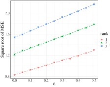
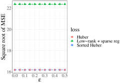
We report simulation results in R with synthetic data demonstrating agreement between theory and practice. The code is in https://github.com/philipthomp/Outlier-robust-regression. We simulate with standard gaussian design entries and gaussian noise. In experiments j) and k) below, $\sigma=0.1$; in the others,we use $\sigma=1$. The purpose of our experiments is threefold. The first is to identify empirically the guarantees of Theorems 2 and 3 for the estimators (12) and (14) with $q=2$. Namely, the linear growth of the mean standard error ($\sqrt{\texttt{MSE}}$) with respect to $\epsilon$ and of the mean squared error (MSE) with respect to $(r,s)$. Secondly, we wish to verify empirically the superiority of “sorted” Huber regression to classical Huber regression. Thirdly, we compare robust estimators with non-robust regularized estimators. Our solvers use a batch version of an alternated proximal gradient method on the separable variables $[\mathbf{B},\boldsymbol{\Gamma},\boldsymbol{\theta}]$. When using the Slope norm, we always set $A=\bar{A}=10$ in the sequences $\boldsymbol{\omega}$ and $\bar{\boldsymbol{\omega}}$. “Huber” and “Sorted Huber” denote Huber regression and Sorted-Huber regression respectively. Due to lack of space, we leave to future work numerical results for the robust estimator (16) regarding adaptation to $\sigma$. We implement the following experiments:

1. We conduct Sorted-Huber sparse linear regression with estimator (14) ($q=2$) with $p=100$, $n=1000$, $s=\{15,25,35\}$ and 100 repetitions. We take $\mathcal{R}$ to be the Slope norm in $\mathbb{R}^{p}$. Respectively, $\boldsymbol{b}^{*}$ and $\boldsymbol{\theta}^{*}$ are set with the first $s$ and $o$ entries equal to $10$ and zero otherwise. See Figure 2(a).

2. Same set-up of a) but with $s=25$ and parameter coordinates with modulus $50$. This time, we compare “Huber” and “Sorted Huber”. See Figure 1. The first 25 entries estimated by “Huber” and “Sorted Huber” fluctuated around $40$ and $48$ respectively.

3. Same set-up of b) but with $\boldsymbol{b}^{*}$ and $\boldsymbol{\theta}^{*}$ having non-zero coordinates set to $1$ and $1000$ respectively. We compare (14) ($q=2$) with sparse regression with Slope norm regularization (“Slope reg”). See Figure 2(b).

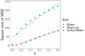
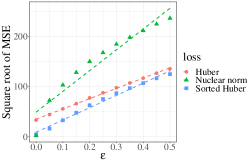
4. We conduct Sorted-Huber low-rank trace regression with estimator (14) ($q=2$) with $d_{1}=d_{2}=10$, $n=1000$, $r=\{1,2,3\}$ and 50 repetitions. We take $\mathcal{R}$ to be the nuclear norm. The low-rank parameter is generated by randomly choosing the spaces of left and right singular vectors with all nonzero singular values equal to $B:=10$. The corruption vector $\boldsymbol{\theta}^{*}$ is set to have the first $o$ entries equal to $M:=10$ and zero otherwise. See Figure 3(a).

5. Same set-up of d) but with $r=5$, $B=M=100$. This time, we compare “Huber” and “Sorted Huber”. See Figure 3(b).

6. Same set-up of e) but with $B=100$ and $M=1000$. We compare estimator (14) ($q=2$) with trace regression with nuclear norm regularization (“Nuclear norm”). See Figure 3(c).

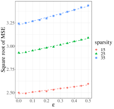
7. We conduct non-corrupted trace regression with additive matrix decomposition ($\epsilon=0$) using estimator (12) with $(\tau,\boldsymbol{\theta})=(0,\mathbf{0})$, $d_{1}=d_{2}=10$, $n=1000$, $s=\{5,80\}$ and 20 repetitions for varying $r$. We take $\mathcal{R}$ and $\mathcal{S}$ to be the nuclear norm and $\ell_{1}$-norm respectively. The low-rank parameter is generated by randomly choosing the spaces of left and right singular vectors such that $\mathsf{a}^{*}=1$. The sparse matrix parameter is simulated with the non-zero entries of value $G:=10$ chosen uniformly at random. See Figure 4(a).

8. Similar set-up of h) but for $r=5$ and varying $s$. See Figure 4(b).

9. We conduct Sorted-Huber trace regression with additive decomposition with estimator (12) for varying $\epsilon$ and three different cases: $(r,s)=(1,5)$, $(r,s)=(3,5)$ and $(r,s)=(5,5)$. The corruption entries are set to $M=1$. The other configurations, except for $(\tau,\boldsymbol{\theta})\neq(0,\mathbf{0})$, are the same as in g). See Figure 5(a).

10. Same set-up of i) but with $\sigma=0.1$, $M=0.5$ and $(r,s)=(1,5)$. This time we compare “Huber” and “Sorted Huber”. See Figure 5(b).

11. Same set-up of j). We compare estimator (12) with trace regression regularized with nuclear norm plus the $\ell_{1}$-norm (“Low-rank + sparse reg”). See Figure 5(c).

The plots identify the linear growth expected from the theory and the superiority of Sorted Huber regression in comparison to Huber regression and non-robust methods.

(a)

(b)

Figure 2: Robust sparse linear regression: different levels of sparsity (a) and comparisons between methods (b).

(a)

(b)

(c)

Figure 3: Robust low-rank trace regression: different values of rank (a), and comparisons between methods (b,c).

(a) Fixed sparsity.

(b) Fixed rank.

Figure 4: Trace regression with additive matrix decomposition with $\epsilon=0$

(a)

(b)

(c)

Figure 5: Robust trace regression with additive decomposition: different values of rank/sparsity (a), and comparisons between methods (b,c).

13 Discussion

We present theoretical and empirical improvements resorting to “sorted” variations of the classical Huber’s loss. Instead of the $\ell_{1}$ norm, the loss in Definition 1 is based on a variational formula regularized by the slope norm — treating each label outlier magnitude individually. This use of the slope norm refines an existing robust loss and should be contrasted to [11, 6]. There, the slope norm is used as a refined regularization norm when estimating the sparse parameter. More generally, this work identifies three design properties, $\operatorname*{PP}$, $\operatorname*{IP}$ and $\operatorname*{MP}$, which jointly entail that the robust estimator (7) is near-optimal in terms of dimension, $\epsilon$ and $\delta$ — when dealing simultaneously with matrix decomposition, label contamination, featured-dependent noise and miss-specification. These properties are based on sharp concentration inequalities stated in Section 7. We believe these could be useful elsewhere, e.g., non-parametric least squares regression [46, 54] and compressive sensing theory [37]. We reemphasize that there seems to be no prior estimation theory for RTRMD — with $\operatorname*{PP}$ being a new application of the product process inequality. Under the incoherence assumption, it would be interesting to investigate further when exact recovery is possible or how nonconvex optimization approaches behave on the model RTRMD [20].

In this supplement we give detailed proofs of the results stated in the main text. It is organized as follows:

• The supplement starts proving Lemmas 9 and 11 and Proposition 2 in Section 8 of the main text — see Sections 14 to 19. Auxiliary lemmas are recalled in Section 20.

• We then pass to the proof of Theorem 15 in Section 10 of the main text. The auxiliary lemmas are proved in order from Sections 21 to 26. The proof of Theorem 15 is concluded in Section 27.

• The proof of Theorem 2 in Section 5 of the main text is given Section 28. It follows from Theorem 15 and Proposition 2. The lower bound — Proposition 1 is proved in Section 29.

• The proof of Theorem 3 in Section 5 in the main text is given in Sections 30 to 32. It also follows Theorem 15 and Proposition 2.

• The proof of Theorem 21 in Section 11 of the main text is presented in Section 33. This theorem and Proposition 2 entail Theorem 4 in Section 5 of the main text — its proof is given in Sections 34 to 36.

• The proofs of Theorems 6 and 7 in Section 7 of the main text and needed peeling lemmas are presented in the Appendix.

Unless otherwise stated, $C>0$ and $c\in(0,1)$ will denote universal constants that may change within the text.

14 Proof of Lemma 9

From $\operatorname*{PP}_{\mathcal{R},\mathcal{R}}(\alpha_{1},\alpha_{2},\alpha_{3},\alpha_{4})$,

$$|\|\mathfrak{X}^{(n)}(\mathbf{V})\|_{2}^{2}-\|\mathbf{V}\|_{\Pi}^{2}| \leq\alpha_{1}\|\mathbf{V}\|_{\Pi}^{2}+(\alpha_{2}+\alpha_{3})\mathcal{R}(\mathbf{V})\|\mathbf{V}\|_{\Pi}+\alpha_{4}\mathcal{R}^{2}(\mathbf{V})$$ (106)

$$\leq\|\mathbf{V}\|_{\Pi}^{2}\left(\alpha_{1}+(\nicefrac{{\alpha^{2}}}{{2}})\right)+\mathcal{R}^{2}(\mathbf{V})\left(\alpha_{4}+\frac{(\alpha_{2}+\alpha_{3})^{2}}{2\alpha^{2}}\right).$$ (107)

Let $0<\alpha<\sqrt{2(1-\alpha_{1})}$. Rearranging and taking the square-root, it follows that $\operatorname*{RSC}_{\mathcal{R}}(\mathsf{a}_{1},\mathsf{a}_{2})$ holds with constants $\mathsf{a}_{1}:=\{1-\alpha_{1}-(\nicefrac{{\alpha^{2}}}{{2}})\}^{1/2}$ and $\mathsf{a}_{2}:=\{\frac{(\alpha_{2}+\alpha_{3})^{2}}{2\alpha^{2}}+\alpha_{4}\}^{1/2}.$ The proof is finished once we set $\alpha^{2}:=(1-\alpha_{1})/2$.

15 Proof of Lemma 11

Let $\alpha:=(\mathsf{a}_{1}\wedge\bar{\mathsf{a}}_{1})/2\sqrt{2}$ and $\beta:=\mathsf{b}_{1}+\mathsf{c}_{1}$. By assumption $b:=\beta+2\alpha^{2}<(\mathsf{a}_{1}\wedge\bar{\mathsf{a}}_{1})^{2}$ and $\mathsf{d}_{1}^{2}=(\mathsf{a}_{1}\wedge\bar{\mathsf{a}}_{1})^{2}-b$. From $\operatorname*{RSC}$,

$$\mathsf{d}_{1}^{2}\|[\mathbf{V},\mathbf{W},\boldsymbol{u}]\|_{\Pi}^{2} \leq\mathsf{a}_{1}^{2}\|\mathbf{V}\|_{\Pi}^{2}+\bar{\mathsf{a}}_{1}^{2}\|\mathbf{W}\|_{\Pi}^{2}+\|\boldsymbol{u}\|_{2}^{2}-b\|[\mathbf{V},\mathbf{W},\boldsymbol{u}]\|_{\Pi}^{2}$$ (108)

$$\leq\left(\|\mathfrak{X}^{(n)}(\mathbf{V})\|_{2}+\mathsf{a}_{2}\mathcal{R}(\mathbf{V})\right)^{2}+\left(\|\mathfrak{X}^{(n)}(\mathbf{W})\|_{2}+\bar{\mathsf{a}}_{2}\mathcal{S}(\mathbf{W})\right)^{2}+\|\boldsymbol{u}\|_{2}^{2}$$ (109)

$$-b\|[\mathbf{V},\mathbf{W},\boldsymbol{u}]\|_{\Pi}^{2},$$ (110)

so, after taking the square-root,

$$\mathsf{d}_{1}\|[\mathbf{V},\mathbf{W},\boldsymbol{u}]\|_{\Pi} \leq\left\{\|\mathfrak{X}^{(n)}(\mathbf{V})\|_{2}^{2}+\|\mathfrak{X}^{(n)}(\mathbf{W})\|_{2}^{2}+\left(\|\boldsymbol{u}\|_{2}^{2}-b\|[\mathbf{V},\mathbf{W},\boldsymbol{u}]\|_{\Pi}^{2}\right)_{+}\right\}^{\frac{1}{2}}$$ (111)

$$+\mathsf{a}_{2}\mathcal{R}(\mathbf{V})+\bar{\mathsf{a}}_{2}\mathcal{S}(\mathbf{W}).$$ (112)

In what follows, it is enough to consider the case $\|\boldsymbol{u}\|_{2}^{2}\geq b\|[\mathbf{V},\mathbf{W},\boldsymbol{u}]\|_{\Pi}^{2}.$

Taking the squares,

$$\|\mathfrak{X}^{(n)}(\mathbf{V})\|_{2}^{2}+\|\mathfrak{X}^{(n)}(\mathbf{W})\|_{2}^{2}+\|\boldsymbol{u}\|_{2}^{2} =\|\mathfrak{X}^{(n)}(\mathbf{V}+\mathbf{W})+\boldsymbol{u}\|_{2}^{2}$$ (113)

$$-2\langle\mathfrak{X}^{(n)}(\mathbf{V}),\mathfrak{X}^{(n)}(\mathbf{W})\rangle-2\langle\mathfrak{X}^{(n)}(\mathbf{V}+\mathbf{W}),\boldsymbol{u}\rangle.$$ (114)

By $\operatorname*{IP}$ and Young’s inequality,

$$T_{1}:=-2\langle\mathfrak{X}^{(n)}(\mathbf{V}+\mathbf{W}),\boldsymbol{u}\rangle \leq 2\mathsf{b}_{1}\left\|[\mathbf{V},\mathbf{W}]\right\|_{\Pi}\|\boldsymbol{u}\|_{2}+2\mathsf{b}_{2}\mathcal{R}(\mathbf{V})\|\boldsymbol{u}\|_{2}$$ (115)

$$+2\mathsf{b}_{3}\mathcal{S}(\mathbf{V})\|\boldsymbol{u}\|_{2}+2\mathsf{b}_{4}\left\|[\mathbf{V},\mathbf{W}]\right\|_{\Pi}\mathcal{Q}(\boldsymbol{u})$$ (116)

$$\leq(\mathsf{b}_{1}+\alpha^{2})(\|[\mathbf{V},\mathbf{W}]\|_{\Pi}^{2}+\|\boldsymbol{u}\|_{2}^{2})+\frac{\mathsf{b}_{2}^{2}}{\alpha^{2}}\mathcal{R}^{2}(\mathbf{V})$$ (117)

$$+\frac{\mathsf{b}_{3}^{2}}{\alpha^{2}}\mathcal{S}^{2}(\mathbf{W})+\frac{\mathsf{b}_{4}^{2}}{\alpha^{2}}\mathcal{Q}^{2}(\boldsymbol{u}).$$ (118)

Let $T_{2}:=-2\langle\mathfrak{X}^{(n)}(\mathbf{V}),\mathfrak{X}^{(n)}(\mathbf{W})\rangle$. By $\operatorname*{PP}$ and Young’s inequality,

$$T_{2}+2\langle\mathchoice{{}\mkern-4.5mu}{{}\mkern-4.5mu}{{}\mkern-2.5mu}{}\langle\mathbf{V},\mathbf{W}\rangle\mathchoice{{}\mkern-4.5mu}{{}\mkern-4.5mu}{{}\mkern-2.5mu}{}\rangle_{\Pi} \leq 2\mathsf{c}_{1}\left\|\mathbf{V}\right\|_{\Pi}\|\mathbf{W}\|_{\Pi}+2\mathsf{c}_{2}\mathcal{R}(\mathbf{V})\|\mathbf{W}\|_{\Pi}+2\mathsf{c}_{3}\left\|\mathbf{V}\right\|_{\Pi}\mathcal{S}(\mathbf{W})$$ (119)

$$+2\gamma\mathsf{c}_{2}\mathsf{c}_{3}\mathcal{R}(\mathbf{V})\mathcal{S}(\mathbf{W})$$ (120)

$$\leq(\mathsf{c}_{1}+\alpha^{2})(\|\mathbf{V}\|_{\Pi}^{2}+\|\mathbf{W}\|_{\Pi}^{2})$$ (121)

$$+\left(\frac{\mathsf{c}_{2}^{2}}{\alpha^{2}}+\gamma\mathsf{c}_{2}^{2}\right)\mathcal{R}^{2}(\mathbf{V})+\left(\frac{\mathsf{c}_{3}^{2}}{\alpha^{2}}+\gamma\mathsf{c}_{3}^{2}\right)\mathcal{S}^{2}(\mathbf{W}).$$ (122)

Let $T_{0}:=\|\mathfrak{X}^{(n)}(\mathbf{V})\|_{2}^{2}+\|\mathfrak{X}^{(n)}(\mathbf{W})\|_{2}^{2}+\|\boldsymbol{u}\|_{2}^{2}$. We thus conclude that

$$T_{0} \leq\|\mathfrak{M}^{(n)}(\mathbf{V}+\mathbf{W},\boldsymbol{u})\|_{2}^{2}-2\langle\mathchoice{{}\mkern-4.5mu}{{}\mkern-4.5mu}{{}\mkern-2.5mu}{}\langle\mathbf{V},\mathbf{W}\rangle\mathchoice{{}\mkern-4.5mu}{{}\mkern-4.5mu}{{}\mkern-2.5mu}{}\rangle_{\Pi}$$ (123)

$$+(\mathsf{b}_{1}+\mathsf{c}_{1}+2\alpha^{2})\|[\mathbf{V},\mathbf{W}]\|_{\Pi}^{2}+(\mathsf{b}_{1}+\alpha^{2})\|\boldsymbol{u}\|_{2}^{2}$$ (124)

$$+\left(\frac{\mathsf{b}_{2}^{2}}{\alpha^{2}}+\frac{\mathsf{c}_{2}^{2}}{\alpha^{2}}+\gamma\mathsf{c}_{2}^{2}\right)\mathcal{R}^{2}(\mathbf{V})+\left(\frac{\mathsf{b}_{3}^{2}}{\alpha^{2}}+\frac{\mathsf{c}_{3}^{2}}{\alpha^{2}}+\gamma\mathsf{c}_{3}^{2}\right)\mathcal{S}^{2}(\mathbf{W})+\frac{\mathsf{b}_{4}^{2}}{\alpha^{2}}\mathcal{Q}^{2}(\boldsymbol{u}).$$ (125)

From (112)-(125) and definitions of $(\beta,b)$,

$$\mathsf{d}_{1}\|[\mathbf{V},\mathbf{W},\boldsymbol{u}]\|_{\Pi} \leq\left\{T_{0}-b\|[\mathbf{V},\mathbf{W},\boldsymbol{u}]\|_{\Pi}^{2}\right\}^{\frac{1}{2}}+\mathsf{a}_{2}\mathcal{R}(\mathbf{V})+\bar{\mathsf{a}}_{2}\mathcal{S}(\mathbf{W})$$ (126)

$$\leq\left\{\|\mathfrak{M}^{(n)}(\mathbf{V}+\mathbf{W},\boldsymbol{u})\|_{2}^{2}-2\langle\mathchoice{{}\mkern-4.5mu}{{}\mkern-4.5mu}{{}\mkern-2.5mu}{}\langle\mathbf{V},\mathbf{W}\rangle\mathchoice{{}\mkern-4.5mu}{{}\mkern-4.5mu}{{}\mkern-2.5mu}{}\rangle_{\Pi}\right\}_{+}^{\frac{1}{2}}$$ (127)

$$+\left(\left\{\frac{\mathsf{b}_{2}^{2}}{\alpha^{2}}+\frac{\mathsf{c}_{2}^{2}}{\alpha^{2}}+\gamma\mathsf{c}_{2}^{2}\right\}^{\frac{1}{2}}+\mathsf{a}_{2}\right)\mathcal{R}(\mathbf{V})+\left(\left\{\frac{\mathsf{b}_{3}^{2}}{\alpha^{2}}+\frac{\mathsf{c}_{3}^{2}}{\alpha^{2}}+\gamma\mathsf{c}_{3}^{2}\right\}^{\frac{1}{2}}+\bar{\mathsf{a}}_{2}\right)\mathcal{S}(\mathbf{W})$$ (128)

$$+\frac{\mathsf{b}_{4}}{\alpha}\mathcal{Q}(\boldsymbol{u}).$$ (129)

16 Proof of Proposition 2, item (i)

We start with the following lemma.

Lemma 22.

Suppose that $\mathbf{X}$ is $L$-subgaussian. Let $\mathcal{B}_{1}$ and $\mathcal{B}_{2}$ be bounded subsets of $\mathbb{B}_{\Pi}$. For any $n\geq 1$ and $t\geq 1$, with probability at least $1-e^{-t}$, it holds that

$$\sup_{[\mathbf{V},\mathbf{W}]\in\mathcal{B}_{1}\times\mathcal{B}_{2}}\left|\langle\mathchoice{{}\mkern-4.5mu}{{}\mkern-4.5mu}{{}\mkern-2.5mu}{}\langle\mathbf{V},\mathbf{W}\rangle\mathchoice{{}\mkern-4.5mu}{{}\mkern-4.5mu}{{}\mkern-2.5mu}{}\rangle_{n}-\langle\mathchoice{{}\mkern-4.5mu}{{}\mkern-4.5mu}{{}\mkern-2.5mu}{}\langle\mathbf{V},\mathbf{W}\rangle\mathchoice{{}\mkern-4.5mu}{{}\mkern-4.5mu}{{}\mkern-2.5mu}{}\rangle_{\Pi}\right| \leq\frac{CL^{2}}{n}\mathscr{G}\big{(}\mathfrak{S}^{1/2}(\mathcal{B}_{1}))\mathscr{G}\big{(}\mathfrak{S}^{1/2}(\mathcal{B}_{2}))$$ (130)

$$+\frac{CL^{2}}{\sqrt{n}}\left[\mathscr{G}\big{(}\mathfrak{S}^{1/2}(\mathcal{B}_{1})+\mathscr{G}\big{(}\mathfrak{S}^{1/2}(\mathcal{B}_{2})\right]$$ (131)

$$+CL^{2}\left(\frac{t}{n}+\sqrt{\frac{t}{n}}\right).$$ (132)

Lemma 22 is immediate from Theorem 7 applied to the classes $F:=\{\mathbf{V}\in\mathcal{B}_{1}:\langle\mathchoice{{}\mkern-4.5mu}{{}\mkern-4.5mu}{{}\mkern-2.5mu}{}\langle\cdot,\mathbf{V}\rangle\mathchoice{{}\mkern-4.5mu}{{}\mkern-4.5mu}{{}\mkern-2.5mu}{}\rangle\}$ and $G:=\{\mathbf{W}\in\mathcal{B}_{2}:\langle\mathchoice{{}\mkern-4.5mu}{{}\mkern-4.5mu}{{}\mkern-2.5mu}{}\langle\cdot,\mathbf{W}\rangle\mathchoice{{}\mkern-4.5mu}{{}\mkern-4.5mu}{{}\mkern-2.5mu}{}\rangle\}$ and Talagrand’s majorizing theorems [83]. The next proposition is a restatement of item (i) of Proposition 2. We prove it using Lemma 22 and the peeling Lemma 35 in Appendix A.

Proposition 4 ($\operatorname*{PP}$).

Suppose that $\mathbf{X}$ is $L$-subgaussian. For all $\delta\in(0,1)$ and $n\in\mathbb{N}$, with probability at least $1-\delta$, the following property holds: for all $[\mathbf{V},\mathbf{W}]\in(\mathds{R}^{p})^{2}$,

$$\left|\langle\mathchoice{{}\mkern-4.5mu}{{}\mkern-4.5mu}{{}\mkern-2.5mu}{}\langle\mathbf{W},\mathbf{V}\rangle\mathchoice{{}\mkern-4.5mu}{{}\mkern-4.5mu}{{}\mkern-2.5mu}{}\rangle_{n}-\langle\mathchoice{{}\mkern-4.5mu}{{}\mkern-4.5mu}{{}\mkern-2.5mu}{}\langle\mathbf{W},\mathbf{V}\rangle\mathchoice{{}\mkern-4.5mu}{{}\mkern-4.5mu}{{}\mkern-2.5mu}{}\rangle_{\Pi}\right| \leq CL^{2}\left(\frac{1+\log(1/\delta)}{n}+\frac{1+\sqrt{\log(1/\delta)}}{\sqrt{n}}\right)\|\mathbf{V}\|_{\Pi}\|\mathbf{W}\|_{\Pi}$$ (133)

$$+CL^{2}\left(\frac{1}{n}+\frac{1}{\sqrt{n}}\right)\mathscr{G}\left(\mathcal{R}(\mathbf{V})\mathfrak{S}^{1/2}(\mathbb{B}_{\mathcal{R}})\cap\|\mathbf{V}\|_{\Pi}\mathbb{B}_{F}\right)\|\mathbf{W}\|_{\Pi}$$ (134)

$$+CL^{2}\left(\frac{1}{n}+\frac{1}{\sqrt{n}}\right)\mathscr{G}\left(\mathcal{S}(\mathbf{W})\mathfrak{S}^{1/2}(\mathbb{B}_{\mathcal{S}})\cap\|\mathbf{W}\|_{\Pi}\mathbb{B}_{F}\right)\big{\|}\mathbf{V}\big{\|}_{\Pi}$$ (135)

$$+\frac{CL^{2}}{n}\mathscr{G}\left(\mathcal{R}(\mathbf{V})\mathfrak{S}^{1/2}(\mathbb{B}_{\mathcal{R}})\cap\|\mathbf{V}\|_{\Pi}\mathbb{B}_{F}\right)\cdot\mathscr{G}\left(\mathcal{S}(\mathbf{W})\mathfrak{S}^{1/2}(\mathbb{B}_{\mathcal{S}})\cap\|\mathbf{W}\|_{\Pi}\mathbb{B}_{F}\right).$$ (136)

Proof.

Let $r,\bar{r}>0$ and define the sets

$$V_{1}:=\{\mathbf{V}:\|\mathbf{V}\|_{\Pi}\leq 1,\mathcal{R}(\mathbf{V})\leq r\},\quad V_{2}:=\{\mathbf{W}:\|\mathbf{W}\|_{\Pi}\leq 1,\mathcal{S}(\mathbf{W})\leq\bar{r}\}.$$ (137)

Note that,

$$\mathscr{G}\left(\mathfrak{S}^{1/2}(V_{1})\right) \leq r\mathscr{G}\left(\mathfrak{S}^{1/2}(\mathbb{B}_{\mathcal{R}})\cap r^{-1}\mathbb{B}_{F}\right)=:g(r),$$ (138)

$$\mathscr{G}\left(\mathfrak{S}^{1/2}(V_{2})\right) \leq\bar{r}\mathscr{G}\left(\mathfrak{S}^{1/2}(\mathbb{B}_{\mathcal{S}})\cap\bar{r}^{-1}\mathbb{B}_{F}\right)=:\bar{g}(\bar{r}).$$ (139)

By Lemma 22, for any $r,\bar{r}>0$ and $\delta\in(0,1/c]$, we have with probability at least $1-c\delta$,

$$\sup_{[\mathbf{V},\mathbf{W}]\in V_{1}\times V_{2}}|\langle\mathchoice{{}\mkern-4.5mu}{{}\mkern-4.5mu}{{}\mkern-2.5mu}{}\langle\mathbf{W},\mathbf{V}\rangle\mathchoice{{}\mkern-4.5mu}{{}\mkern-4.5mu}{{}\mkern-2.5mu}{}\rangle_{n}-\langle\mathchoice{{}\mkern-4.5mu}{{}\mkern-4.5mu}{{}\mkern-2.5mu}{}\langle\mathbf{W},\mathbf{V}\rangle\mathchoice{{}\mkern-4.5mu}{{}\mkern-4.5mu}{{}\mkern-2.5mu}{}\rangle_{\Pi}| \leq\frac{CL^{2}}{n}\cdot g(r)\bar{g}(\bar{r})+\frac{CL^{2}}{\sqrt{n}}[g(r)+\bar{g}(\bar{r})]$$ (140)

$$+CL^{2}\left(\sqrt{\frac{\log(1/\delta)}{n}}+\frac{\log(1/\delta)}{n}\right).$$ (141)

We now invoke Lemma 35 with the set $V:=\mathbb{B}_{\Pi}\times\mathbb{B}_{\Pi}$, functions

$$M(\mathbf{V},\mathbf{W}) :=-\left|\langle\mathchoice{{}\mkern-4.5mu}{{}\mkern-4.5mu}{{}\mkern-2.5mu}{}\langle\mathbf{W},\mathbf{V}\rangle\mathchoice{{}\mkern-4.5mu}{{}\mkern-4.5mu}{{}\mkern-2.5mu}{}\rangle_{n}-\langle\mathchoice{{}\mkern-4.5mu}{{}\mkern-4.5mu}{{}\mkern-2.5mu}{}\langle\mathbf{W},\mathbf{V}\rangle\mathchoice{{}\mkern-4.5mu}{{}\mkern-4.5mu}{{}\mkern-2.5mu}{}\rangle_{\Pi}\right|,$$ (142)

$$h(\mathbf{V},\mathbf{W}) :=\mathcal{R}(\mathbf{V})$$ (143)

$$\bar{h}(\mathbf{V},\mathbf{W}) :=\mathcal{S}(\mathbf{W}),$$ (144)

functions $g$ and $\bar{g}$ as stated above and constant $b:=CL^{2}$. The claim follows from such lemma and the homogeneity of norms. ∎

17 Proof of Proposition 2, item (ii)

By item (i) of Proposition 2, with probability$\geq 1-\delta$, $\operatorname*{PP}_{\mathcal{R},\mathcal{R}}$ holds with constants

$$\mathsf{c}_{1} =CL^{2}\left(\frac{1+\log(1/\delta)}{n}+\frac{1+\sqrt{\log(1/\delta)}}{\sqrt{n}}\right),$$ (145)

$$\mathsf{c}_{2}=\mathsf{c}_{3} =CL^{2}\left(\frac{1}{n}+\frac{1}{\sqrt{n}}\right)\mathscr{G}\left(\mathfrak{S}^{1/2}(\mathbb{B}_{\mathcal{R}})\right),$$ (146)

$$\mathsf{c}_{4} =\frac{CL^{2}}{n}\mathscr{G}^{2}\left(\mathfrak{S}^{1/2}(\mathbb{B}_{\mathcal{R}})\right).$$ (147)

The claim follows from this and Lemma 9 with constant $\alpha^{2}=(1-\mathsf{c}_{1})/2$ — noting that, by assumption $\mathsf{c}_{1}\in(0,1)$.

18 Proof of Proposition 2, item (iii)

We start with the following lemma, stating a high-probability version of Chevet’s inequality. This result is suggested as an exercise in Vershynin [1]. We give a proof for completeness.

Lemma 23.

Suppose that $\mathbf{X}$ is $L$-subgaussian. Let $V$ be any bounded subset of $\mathbb{B}_{\Pi}\times\mathbb{B}_{2}^{n}$ Define $V_{1}:=\{\mathbf{V}:\exists\,\boldsymbol{u}\text{ s.t. }(\mathbf{V},\boldsymbol{u})\in V\}$ and $V_{2}:=\{\boldsymbol{u}:\exists\,\mathbf{V}\text{ s.t. }(\mathbf{V},\boldsymbol{u})\in V\}$.

Then, for any $n\geq 1$ and $t>0$, with probability at least $1-2\exp(-t^{2})$,

$$\sup_{[\mathbf{V},\boldsymbol{u}]\in V}\langle\boldsymbol{u},\mathfrak{X}(\mathbf{V})\rangle\leq CL[\mathscr{G}\big{(}\mathfrak{S}^{1/2}(V_{1}))+\mathscr{G}\big{(}V_{2}\big{)}+t].$$

Proof.

For each $(\mathbf{V},\boldsymbol{u})\in V$, we define

$$Z_{\mathbf{V},\boldsymbol{u}} :=\langle\boldsymbol{u},\mathfrak{X}(\mathbf{V})\rangle=\sum_{i\in[n]}\boldsymbol{u}_{i}\langle\mathchoice{{}\mkern-4.5mu}{{}\mkern-4.5mu}{{}\mkern-2.5mu}{}\langle\mathbf{X}_{i},\mathbf{V}\rangle\mathchoice{{}\mkern-4.5mu}{{}\mkern-4.5mu}{{}\mkern-2.5mu}{}\rangle,\qquad W_{\mathbf{V},\boldsymbol{u}}:=L(\langle\mathchoice{{}\mkern-4.5mu}{{}\mkern-4.5mu}{{}\mkern-2.5mu}{}\langle\mathbf{V},\mathfrak{S}^{1/2}(\boldsymbol{\Xi})\rangle\mathchoice{{}\mkern-4.5mu}{{}\mkern-4.5mu}{{}\mkern-2.5mu}{}\rangle+\langle\boldsymbol{u},\boldsymbol{\xi}\rangle),$$ (148)

where $\boldsymbol{\Xi}\in\mathds{R}^{p}$ and $\boldsymbol{\xi}\in\mathbb{R}^{n}$ are independent each one having iid $\mathcal{N}(0,1)$ entries. Therefore, $(\mathbf{V},\boldsymbol{u})\mapsto W_{\mathbf{V},\boldsymbol{u}}$ defines a centered Gaussian process indexed by $V$.

We may easily bound the $\psi_{2}$-norm of the increments using rotation invariance of sub-Gaussian random variables. Indeed, using that $\{\mathbf{X}_{i}\}$ is an iid sequence and Proposition 2.6.1 in [1], given $[\mathbf{V},\boldsymbol{u}]$ and $[\mathbf{V}^{\prime},\boldsymbol{u}^{\prime}]$ in $V$,

$$|Z_{\mathbf{V},\boldsymbol{u}}-Z_{\mathbf{V}^{\prime},\boldsymbol{u}^{\prime}}|_{\psi_{2}}^{2} =\left|\sum_{i\in[n]}\langle\mathchoice{{}\mkern-4.5mu}{{}\mkern-4.5mu}{{}\mkern-2.5mu}{}\langle\mathbf{X}_{i},\boldsymbol{u}_{i}\mathbf{V}-\boldsymbol{u}^{\prime}_{i}\mathbf{V}^{\prime}\rangle\mathchoice{{}\mkern-4.5mu}{{}\mkern-4.5mu}{{}\mkern-2.5mu}{}\rangle\right|_{\psi_{2}}^{2}$$ (149)

$$\leq C\sum_{i\in[n]}\left|\langle\mathchoice{{}\mkern-4.5mu}{{}\mkern-4.5mu}{{}\mkern-2.5mu}{}\langle\mathbf{X}_{i},\boldsymbol{u}_{i}\mathbf{V}-\boldsymbol{u}_{i}^{\prime}\mathbf{V}^{\prime}\rangle\mathchoice{{}\mkern-4.5mu}{{}\mkern-4.5mu}{{}\mkern-2.5mu}{}\rangle\right|_{\psi_{2}}^{2}$$ (150)

$$\leq 2C\sum_{i\in[n]}\left|\langle\mathchoice{{}\mkern-4.5mu}{{}\mkern-4.5mu}{{}\mkern-2.5mu}{}\langle\mathbf{X}_{i},(\boldsymbol{u}_{i}-\boldsymbol{u}_{i}^{\prime})\mathbf{V}\rangle\mathchoice{{}\mkern-4.5mu}{{}\mkern-4.5mu}{{}\mkern-2.5mu}{}\rangle\right|^{2}_{\psi_{2}}+2C\sum_{i\in[n]}\left|\langle\mathchoice{{}\mkern-4.5mu}{{}\mkern-4.5mu}{{}\mkern-2.5mu}{}\langle\mathbf{X}_{i},\boldsymbol{u}_{i}^{\prime}(\mathbf{V}-\mathbf{V}^{\prime})\rangle\mathchoice{{}\mkern-4.5mu}{{}\mkern-4.5mu}{{}\mkern-2.5mu}{}\rangle\right|_{\psi_{2}}^{2}$$ (151)

$$\leq 2CL^{2}\|\boldsymbol{u}-\boldsymbol{u}^{\prime}\|_{2}^{2}\|\mathbf{V}\|_{\Pi}^{2}+2CL^{2}\|\boldsymbol{u}^{\prime}\|_{2}^{2}\|\mathbf{V}-\mathbf{V}^{\prime}\|_{\Pi}^{2}\leq 2CL^{2}\mathsf{d}([\mathbf{V},\boldsymbol{u}],[\mathbf{V}^{\prime},\boldsymbol{u}^{\prime}]),$$ (152)

with the pseudo-metric $\mathsf{d}([\mathbf{V},\boldsymbol{u}],[\mathbf{V}^{\prime},\boldsymbol{u}^{\prime}]):=\sqrt{\|\boldsymbol{u}-\boldsymbol{u}^{\prime}\|_{2}^{2}+\|\mathbf{V}-\mathbf{V}^{\prime}\|_{\Pi}^{2}}$, using that $\|\mathbf{V}\|_{\Pi}\leq 1$ and $\|\boldsymbol{u}^{\prime}\|_{2}\leq 1$. On the other hand, by definition of the process $W$ it is easy to check that

$$\mathbb{E}[(W_{\mathbf{V},\boldsymbol{u}}-W_{\mathbf{V}^{\prime},\boldsymbol{u}^{\prime}})^{2}]=L^{2}(\|\mathbf{V}-\mathbf{V}^{\prime}\|_{\Pi}^{2}+\|\boldsymbol{u}-\boldsymbol{u}^{\prime}\|_{2}^{2}).$$ (153)

From (152),(153), we conclude that the processes $W$ and $Z$ satisfy the conditions of Talagrand’s majoration and minoration generic chaining bounds for sub-Gaussian processes (e.g. Theorems 8.5.5 and 8.6.1 in [1]). Hence, for any $t\geq 0$, with probability at least $1-2e^{-t^{2}}$,

$$\sup_{[\mathbf{V},\boldsymbol{u}]\in V}|Z_{\mathbf{V},\boldsymbol{u}}|\leq CL\left\{\mathbb{E}\left[\sup_{[\mathbf{V},\boldsymbol{u}]\in V}W_{\mathbf{V},\boldsymbol{u}}\right]+t\right\}.$$ (154)

In above we used that $Z_{\mathbf{V}_{0},\boldsymbol{u}_{0}}=0$ at $[\mathbf{V}_{0},\boldsymbol{u}_{0}]=0$ and that the diameter of $V\subset\mathbb{B}_{\Pi}^{m_{1}\times m_{2}}\times\mathbb{B}_{2}^{n}$ under the metric $\mathsf{d}$ is less than $2\sqrt{2}$. We also have

$$\mathbb{E}\bigg{[}\sup_{[\mathbf{V},\boldsymbol{u}]\in V}W_{\mathbf{V},\boldsymbol{u}}\bigg{]}\leq\mathbb{E}\bigg{[}\sup_{\mathbf{V}\in V_{1}}\langle\mathchoice{{}\mkern-4.5mu}{{}\mkern-4.5mu}{{}\mkern-2.5mu}{}\langle\boldsymbol{\Xi},\mathfrak{S}^{1/2}(\mathbf{V})\rangle\mathchoice{{}\mkern-4.5mu}{{}\mkern-4.5mu}{{}\mkern-2.5mu}{}\rangle\bigg{]}+\mathbb{E}\bigg{[}\sup_{\boldsymbol{u}\in V_{2}}\langle\boldsymbol{u},\boldsymbol{\xi}\rangle\bigg{]}=\mathscr{G}\big{(}\mathfrak{S}^{1/2}(V_{1}))+\mathscr{G}(V_{2}).$$ (155)

Joining the two previous inequalities complete the proof of the claimed inequality. ∎

The next proposition is a restatement of item (iii) of Proposition 2. We prove it using Lemma 23 and the peeling Lemma 36 in Appendix A.

Proposition 5 ($\operatorname*{IP}$).

Suppose that $\mathbf{X}$ is $L$-subgaussian. For all $\delta\in(0,1)$ and $n\in\mathbb{N}$, with probability at least $1-\delta$, the following property holds: for all $[\mathbf{V},\mathbf{W},\boldsymbol{u}]\in(\mathds{R}^{p})^{2}\times\mathbb{R}^{n}$,

$$\langle\boldsymbol{u},\mathfrak{X}^{(n)}(\mathbf{V}+\mathbf{W})\rangle \leq CL\frac{1+\sqrt{\log(1/\delta)}}{\sqrt{n}}\|[\mathbf{V},\mathbf{W}]\|_{\Pi}\|\boldsymbol{u}\|_{2}$$ (156)

$$+CL\frac{\mathscr{G}\big{(}\mathcal{R}(\mathbf{V})\mathfrak{S}^{1/2}(\mathbb{B}_{\mathcal{R}})\cap\|[\mathbf{V},\mathbf{W}]\|_{\Pi}\mathbb{B}_{F}\big{)}}{\sqrt{n}}\|\boldsymbol{u}\|_{2}$$ (157)

$$+CL\frac{\mathscr{G}\big{(}\mathcal{S}(\mathbf{W})\mathfrak{S}^{1/2}(\mathbb{B}_{\mathcal{S}})\cap\|[\mathbf{V},\mathbf{W}]\|_{\Pi}\mathbb{B}_{F}\big{)}}{\sqrt{n}}\|\boldsymbol{u}\|_{2}$$ (158)

$$+CL\frac{\mathscr{G}\big{(}\mathcal{Q}(\boldsymbol{u})\mathbb{B}_{\mathcal{Q}}\cap\|\boldsymbol{u}\|_{2}\mathbb{B}_{2}^{n}\big{)}}{\sqrt{n}}\|[\mathbf{V},\mathbf{W}]\|_{\Pi}.$$ (159)

Proof.

Let $R_{1},R_{2},R_{3}>0$ and define the sets

$$V_{1} :=\{\mathbf{V}\in\mathds{R}^{p}:\|\mathbf{V}\|_{\Pi}\leq 1,\mathcal{R}(\mathbf{V})\leq R_{1}\},$$ (160)

$$V_{2} :=\{\boldsymbol{u}\in\mathbb{R}^{n}:\|\boldsymbol{u}\|_{2}\leq 1,\mathcal{Q}(\boldsymbol{u})\leq R_{2}\},$$ (161)

$$V_{3} :=\{\mathbf{W}\in\mathds{R}^{p}:\|\mathbf{W}\|_{\Pi}\leq 1,\mathcal{S}(\mathbf{V})\leq R_{3}\}.$$ (162)

We note that

$$\mathscr{G}\left(\mathfrak{S}^{1/2}(V_{1})\right) \leq R_{1}\mathscr{G}\left(\mathfrak{S}^{1/2}(\mathbb{B}_{\mathcal{R}})\cap R_{1}^{-1}\mathbb{B}_{F}\right)=:g_{1}(R_{1}),$$ (163)

$$\mathscr{G}(V_{2}) \leq R_{2}\mathscr{G}\left(\mathbb{B}_{\mathcal{Q}}\cap R_{2}^{-1}\mathbb{B}_{2}^{n}\right)=:g_{2}(R_{2}),$$ (164)

$$\mathscr{G}\left(\mathfrak{S}^{1/2}(V_{3})\right) \leq R_{3}\mathscr{G}\left(\mathfrak{S}^{1/2}(\mathbb{B}_{\mathcal{S}})\cap R_{3}^{-1}\mathbb{B}_{F}\right)=:g_{3}(R_{3}).$$ (165)

By Lemma 23, we have that, for any $R_{1},R_{2}>0$ and $\delta\in(0,1)$, with probability at least $1-\delta$, the following inequality holds:

$$\sup_{[\mathbf{V},\boldsymbol{u}]\in V_{1}\times V_{2}}\langle\boldsymbol{u},\mathfrak{X}^{(n)}(\mathbf{V})\rangle \leq\frac{CL}{\sqrt{n}}g_{1}(R_{1})+\frac{CL}{\sqrt{n}}g_{2}(R_{2})+\frac{CL}{\sqrt{n}}\sqrt{\log(2/\delta)}.$$ (166)

Next, we invoke Lemma 36 with the set $V:=\mathbb{B}_{\Pi}\times\mathbb{B}_{2}^{n}$, functions

$$M(\mathbf{V},\boldsymbol{u}) :=-\langle\boldsymbol{u},\mathfrak{X}^{(n)}(\mathbf{V})\rangle,$$ (167)

$$h(\mathbf{V},\boldsymbol{u}) :=\mathcal{R}(\mathbf{V})$$ (168)

$$\bar{h}(\mathbf{V},\boldsymbol{u}) :=\mathcal{Q}(\boldsymbol{u}),$$ (169)

functions $g:=g_{1}$ and $\bar{g}:=g_{2}$ and constant $b:=CL$. By this lemma, given $\delta\in(0,1)$, with probability at least $1-\delta$, for all $[\mathbf{V},\boldsymbol{u}]\in\mathbb{B}_{\Pi}\times\mathbb{B}_{2}^{n}$,

$$\langle\boldsymbol{u},\mathfrak{X}^{(n)}(\mathbf{V})\rangle \leq\frac{CL}{\sqrt{n}}\mathscr{G}\left(\mathcal{R}(\mathbf{V})\mathfrak{S}^{1/2}(\mathbb{B}_{\mathcal{R}})\cap\mathbb{B}_{F}\right)$$ (170)

$$+\frac{CL}{\sqrt{n}}\mathscr{G}\left(\mathcal{Q}(\boldsymbol{u})\mathbb{B}_{\mathcal{Q}}\cap\mathbb{B}_{2}^{n}\right)$$ (171)

$$+\frac{CL}{\sqrt{n}}(1+\sqrt{\log(1/\delta)}).$$ (172)

Similarly, we will invoke Lemma 23 with set $V_{3}\times V_{2}$ and Lemma 36 with set $V:=\mathbb{B}_{\Pi}\times\mathbb{B}_{2}^{n}$, functions

$$M(\mathbf{W},\boldsymbol{u}) :=-\langle\boldsymbol{u},\mathfrak{X}^{(n)}(\mathbf{W})\rangle,$$ (173)

$$h(\mathbf{W},\boldsymbol{u}) :=\mathcal{S}(\mathbf{V})$$ (174)

$$\bar{h}(\mathbf{W},\boldsymbol{u}) :=\mathcal{Q}(\boldsymbol{u}),$$ (175)

functions $g:=g_{3}$ and $\bar{g}:=g_{2}$ and constant $b:=CL$. We obtain that, for any $\delta\in(0,1)$, with probability at least $1-\delta$, for all $[\mathbf{W},\boldsymbol{u}]\in\mathbb{B}_{\Pi}\times\mathbb{B}_{2}^{n}$,

$$\langle\boldsymbol{u},\mathfrak{X}^{(n)}(\mathbf{W})\rangle \leq\frac{CL}{\sqrt{n}}\mathscr{G}\left(\mathcal{S}(\mathbf{W})\mathfrak{S}^{1/2}(\mathbb{B}_{\mathcal{S}})\cap\mathbb{B}_{F}\right)$$ (176)

$$+\frac{CL}{\sqrt{n}}\mathscr{G}\left(\mathcal{Q}(\boldsymbol{u})\mathbb{B}_{\mathcal{Q}}\cap\mathbb{B}_{2}^{n}\right)$$ (177)

$$+\frac{CL}{\sqrt{n}}(1+\sqrt{\log(1/\delta)}).$$ (178)

By an union bound, we obtain that, for every $\delta\in(0,1)$, with probability at least $1-\delta$, for all $[\mathbf{V},\mathbf{W},\boldsymbol{u}]\in\mathbb{B}_{\Pi}\times\mathbb{B}_{\Pi}\times\mathbb{B}_{2}^{n}$,

$$\langle\boldsymbol{u},\mathfrak{X}^{(n)}(\mathbf{V}+\mathbf{W})\rangle \leq\frac{CL}{\sqrt{n}}\mathscr{G}\left(\mathcal{R}(\mathbf{V})\mathfrak{S}^{1/2}(\mathbb{B}_{\mathcal{R}})\cap\mathbb{B}_{F}\right)+\frac{CL}{\sqrt{n}}\mathscr{G}\left(\mathcal{S}(\mathbf{W})\mathfrak{S}^{1/2}(\mathbb{B}_{\mathcal{S}})\cap\mathbb{B}_{F}\right)$$ (179)

$$+\frac{2CL}{\sqrt{n}}\mathscr{G}\left(\mathcal{Q}(\boldsymbol{u})\mathbb{B}_{\mathcal{Q}}\cap\mathbb{B}_{2}^{n}\right)$$ (180)

$$+\frac{2CL}{\sqrt{n}}(1+\sqrt{\log(1/\delta)}).$$ (181)

To finish, we use that, for any $[\mathbf{V},\mathbf{W},\boldsymbol{u}]$ with non-zero coordinates, $\left[\frac{\mathbf{V}}{\|[\mathbf{V},\mathbf{W}]\|_{\Pi}},\frac{\mathbf{W}}{\|[\mathbf{V},\mathbf{W}]\|_{\Pi}},\frac{\boldsymbol{u}}{\|\boldsymbol{u}\|_{2}}\right]$ belongs $\mathbb{B}_{\Pi}\times\mathbb{B}_{\Pi}\times\mathbb{B}_{2}^{n}$ and use homogeneity of norms. ∎

19 Proof of Proposition 2, item (iv)

We start by stating two auxiliary lemmas. The next result follows from a tail symmetrization-contraction argument and the Gaussian concentration inequality.

Lemma 24 (Proposition 9.2 in [6]).

Assume $\sigma:=|\xi|_{\psi_{2}}<\infty$. Let $U$ be any bounded subset of $\mathbb{B}^{n}_{2}$. For any $n\geq 1$ and $t>0$, with probability at least $1-\exp(-t^{2}/2)$,

$$\sup_{\boldsymbol{u}\in U}\langle\boldsymbol{\xi},\boldsymbol{u}\rangle\leq C\sigma\left[\mathscr{G}\big{(}U\big{)}+t\right].$$

Next, we state the following lemma.

Lemma 25.

Suppose that $\mathbf{X}$ is $L$-subgaussian. Let $V$ be a bounded subset of $\mathbb{B}_{\Pi}$. There exists universal constant $c>0$, such that for all $n\geq 1$, $u,v\geq 1$, with probability at least $1-ce^{-u/4}-ce^{-nv}$,

$$\sup_{\mathbf{V}\in V}\langle\boldsymbol{\xi}^{(n)},\mathfrak{X}^{(n)}(\mathbf{V})\rangle \leq C\left(\sqrt{v}+1\right)\frac{\sigma L}{\sqrt{n}}\mathscr{G}\big{(}\mathfrak{S}^{1/2}(V))+C\sigma L\left(\sqrt{\frac{2u}{n}}+\frac{u}{n}+\sqrt{\frac{uv}{n}}\right).$$ (182)

The previous lemma is immediate from Theorem 6 applied to the class $F:=\{\mathbf{V}\in\mathcal{B}:\langle\mathchoice{{}\mkern-4.5mu}{{}\mkern-4.5mu}{{}\mkern-2.5mu}{}\langle\cdot,\mathbf{V}\rangle\mathchoice{{}\mkern-4.5mu}{{}\mkern-4.5mu}{{}\mkern-2.5mu}{}\rangle\}$ and Talagrand’s majorizing theorems.

Finally, the next proposition is a restatement of item (iv) of Proposition 2. We prove it using Lemmas 24 and 25 and two peeling lemmas: Lemma 36 (with $\bar{g}=\bar{h}\equiv 0$) and Lemma 37 in Appendix A. We recall the following definition:

$$\triangle_{n}(\delta) :=(\nicefrac{{1}}{{\sqrt{n}}})[1+\sqrt{\log(1/\delta)}]+(\nicefrac{{1}}{{n}})[1+\log(1/\delta)+\sqrt{\log(1/\delta)}].$$ (183)

Next, we also define the functions

$$g_{\mathcal{R}}(\mathbf{V},\mathbf{W},\boldsymbol{u}) :=\mathscr{G}\left(\mathcal{R}(\mathbf{V})\mathfrak{S}^{1/2}(\mathbb{B}_{\mathcal{R}})\cap\|[\mathbf{V},\mathbf{W},\boldsymbol{u}]\|_{\Pi}\mathbb{B}_{F}\right),$$ (184)

$$g_{\mathcal{S}}(\mathbf{V},\mathbf{W},\boldsymbol{u}) :=\mathscr{G}\left(\mathcal{S}(\mathbf{W})\mathfrak{S}^{1/2}(\mathbb{B}_{\mathcal{S}})\cap\|[\mathbf{V},\mathbf{W},\boldsymbol{u}]\|_{\Pi}\mathbb{B}_{F}\right),$$ (185)

$$g_{\mathcal{Q}}(\mathbf{V},\mathbf{W},\boldsymbol{u}) :=\mathscr{G}\left(\mathcal{Q}(\boldsymbol{u})\mathbb{B}_{\mathcal{Q}}\cap\|[\mathbf{V},\mathbf{W},\boldsymbol{u}]\|_{\Pi}\mathbb{B}_{2}^{n}\right).$$ (186)

Proposition 6 ($\operatorname*{MP}$).

For all $n\in\mathbb{N}$ and all $\delta\in(0,1)$, with probability at least $1-\delta$, for all $[\mathbf{V},\mathbf{W},\boldsymbol{u}]\in\mathbb{B}_{\Pi}\times\mathbb{B}_{\Pi}\times\mathbb{B}_{2}^{n}$,

$$\langle\boldsymbol{\xi}^{(n)},\mathfrak{M}^{(n)}(\mathbf{V}+\mathbf{W},\boldsymbol{u})\rangle \leq C\sigma L\cdot\triangle_{n}(\delta)\cdot\|[\mathbf{V},\mathbf{W},\boldsymbol{u}]\|_{\Pi}$$ (187)

$$+C\sigma L\left\{[1+(\nicefrac{{1}}{{\sqrt{n}}})\sqrt{\log(1/\delta)}]\frac{1}{\sqrt{n}}+\frac{1}{n}\right\}g_{\mathcal{R}}(\mathbf{V},\mathbf{W},\boldsymbol{u})$$ (188)

$$+C\sigma L\left\{[1+(\nicefrac{{1}}{{\sqrt{n}}})\sqrt{\log(1/\delta)}]\frac{1}{\sqrt{n}}+\frac{1}{n}\right\}g_{\mathcal{S}}(\mathbf{V},\mathbf{W},\boldsymbol{u})$$ (189)

$$+C\frac{\sigma}{\sqrt{n}}g_{\mathcal{Q}}(\mathbf{V},\mathbf{W},\boldsymbol{u}).$$ (190)

Proof.

Given $R_{1},R_{2},R_{3}>0$, we recall the definitions of the sets $V_{1}$, $V_{2}$ and $V_{3}$ in (160), (161) and (162) and functions $g_{1}$, $g_{2}$ and $g_{3}$ in (163), (164) and (165).

By Lemma 25, there is constant $c\geq 1$, such that, for any $R_{1}>0$ and $\delta\in(0,1/c]$, with probability at least $1-2c\delta$,

$$\sup_{\mathbf{V}\in V_{1}}\langle\boldsymbol{\xi}^{(n)},\mathfrak{X}^{(n)}(\mathbf{V})\rangle \leq C\left(\sqrt{\frac{\log(1/\delta)}{n}}+1\right)\frac{\sigma L}{\sqrt{n}}g_{1}(R_{1})$$ (191)

$$+C\sigma L\left(\sqrt{\frac{\log(1/\delta)}{n}}+\frac{\log(1/\delta)}{n}\right).$$ (192)

Next, we invoke Lemma 37 with the set $V:=\mathbb{B}_{\Pi}$, functions

$$M(\mathbf{V}) :=-\langle\boldsymbol{\xi}^{(n)},\mathfrak{X}^{(n)}(\mathbf{V})\rangle,$$ (193)

$$h(\mathbf{V}) :=\mathcal{R}(\mathbf{V}),$$ (194)

function $g:=g_{1}$ and constant $b:=C\sigma L$. By this lemma, given $\delta\in(0,1/2c]$, with probability at least $1-2c\delta$, for all $\mathbf{V}\in\mathbb{B}_{\Pi}$,

$$\langle\boldsymbol{\xi}^{(n)},\mathfrak{X}^{(n)}(\mathbf{V})\rangle \leq C\left\{[1+(\nicefrac{{1}}{{\sqrt{n}}})\sqrt{\log(1/\delta)}]\frac{\sigma L}{\sqrt{n}}+\frac{\sigma L}{n}\right\}\mathscr{G}\left(\mathcal{R}(\mathbf{V})\mathfrak{S}^{1/2}(\mathbb{B}_{\mathcal{R}})\cap\mathbb{B}_{F}\right)$$ (195)

$$+C(\nicefrac{{\sigma L}}{{\sqrt{n}}})[1+\sqrt{\log(1/\delta)}]+C(\nicefrac{{\sigma L}}{{n}})[\log(1/\delta)+\sqrt{\log(1/\delta)}].$$ (196)

Proceeding exactly like above but with set $V_{3}$, norm $\mathcal{S}$ and function $g:=g_{3}$, we get that for all $\delta\in(0,1/2c]$, with probability at least $1-2c\delta$, for all $\mathbf{W}\in\mathbb{B}_{\Pi}$,

$$\langle\boldsymbol{\xi}^{(n)},\mathfrak{X}^{(n)}(\mathbf{W})\rangle \leq C\left\{[1+(\nicefrac{{1}}{{\sqrt{n}}})\sqrt{\log(1/\delta)}]\frac{\sigma L}{\sqrt{n}}+\frac{\sigma L}{n}\right\}\mathscr{G}\left(\mathcal{S}(\mathbf{W})\mathfrak{S}^{1/2}(\mathbb{B}_{\mathcal{S}})\cap\mathbb{B}_{F}\right)$$ (197)

$$+C(\nicefrac{{\sigma L}}{{\sqrt{n}}})[1+\sqrt{\log(1/\delta)}]+C(\nicefrac{{\sigma L}}{{n}})[\log(1/\delta)+\sqrt{\log(1/\delta)}].$$ (198)

Finally, by Lemma 24, for any $R_{2}>0$ and $\delta\in(0,1)$, with probability at least $1-\delta$,

$$\sup_{\boldsymbol{u}\in V_{2}}\langle\boldsymbol{\xi}^{(n)},\boldsymbol{u}\rangle\leq C\frac{\sigma}{\sqrt{n}}\left[g_{2}(R_{2})+\sqrt{\log(1/\delta)}\right].$$ (199)

We now invoke Lemma 36 with set $V:=\mathbb{B}_{2}^{n}$, functions

$$M(\boldsymbol{u}) :=-\langle\boldsymbol{\xi}^{(n)},\boldsymbol{u}\rangle,$$ (200)

$$h(\boldsymbol{u}) :=\mathcal{Q}(\boldsymbol{u}),$$ (201)

function $g:=g_{2}$ (and $\bar{g}=\bar{h}\equiv 0$) and constant $b:=C\sigma$. We get that, for any $\delta\in(0,1)$, with probability at least $1-\delta$, for all $\boldsymbol{u}\in\mathbb{B}_{2}^{n}$,

$$\langle\boldsymbol{\xi}^{(n)},\boldsymbol{u}\rangle\leq C\frac{\sigma}{\sqrt{n}}\mathscr{G}\left(\mathcal{Q}(\boldsymbol{u})\mathbb{B}_{\mathcal{Q}}\cap\mathbb{B}_{2}^{n}\right)+C\frac{\sigma}{\sqrt{n}}\left[1+\sqrt{\log(1/\delta)}\right].$$ (202)

By an union bound, we obtain that, for every $\delta\in(0,1/(4c+1)]$, with probability at least $1-(4c+1)\delta$, for all $[\mathbf{V},\mathbf{W},\boldsymbol{u}]\in\mathbb{B}_{\Pi}\times\mathbb{B}_{\Pi}\times\mathbb{B}_{2}^{n}$,

$$\langle\boldsymbol{\xi}^{(n)},\mathfrak{M}^{(n)}(\mathbf{V}+\mathbf{W},\boldsymbol{u})\rangle =\langle\boldsymbol{\xi}^{(n)},\mathfrak{X}^{(n)}(\mathbf{V})\rangle+\langle\boldsymbol{\xi}^{(n)},\mathfrak{X}^{(n)}(\mathbf{W})\rangle+\langle\boldsymbol{\xi}^{(n)},\boldsymbol{u}\rangle$$ (203)

$$\leq C\left\{[1+(\nicefrac{{1}}{{\sqrt{n}}})\sqrt{\log(1/\delta)}]\frac{\sigma L}{\sqrt{n}}+\frac{\sigma L}{n}\right\}\mathscr{G}\left(\mathcal{R}(\mathbf{V})\mathfrak{S}^{1/2}(\mathbb{B}_{\mathcal{R}})\cap\mathbb{B}_{F}\right)$$ (204)

$$+C\left\{[1+(\nicefrac{{1}}{{\sqrt{n}}})\sqrt{\log(1/\delta)}]\frac{\sigma L}{\sqrt{n}}+\frac{\sigma L}{n}\right\}\mathscr{G}\left(\mathcal{S}(\mathbf{V})\mathfrak{S}^{1/2}(\mathbb{B}_{\mathcal{S}})\cap\mathbb{B}_{F}\right)$$ (205)

$$+C\frac{\sigma}{\sqrt{n}}\mathscr{G}\left(\mathcal{Q}(\boldsymbol{u})\mathbb{B}_{\mathcal{Q}}\cap\mathbb{B}_{2}^{n}\right)$$ (206)

$$+3C(\nicefrac{{\sigma L}}{{\sqrt{n}}})[1+\sqrt{\log(1/\delta)}]+2C(\nicefrac{{\sigma L}}{{n}})[\log(1/\delta)+\sqrt{\log(1/\delta)}],$$ (207)

where we used that $L\geq 1$.

To finish, we use that, for any $[\mathbf{V},\mathbf{W},\boldsymbol{u}]$ with non-zero coordinates, the vector

$$\left[\frac{\mathbf{V}}{\|[\mathbf{V},\mathbf{W},\boldsymbol{u}]\|_{\Pi}},\frac{\mathbf{W}}{\|[\mathbf{V},\mathbf{W},\boldsymbol{u}]\|_{\Pi}},\frac{\boldsymbol{u}}{\|[\mathbf{V},\mathbf{W},\boldsymbol{u}]\|_{\Pi}}\right]$$

belongs to $\mathbb{B}_{\Pi}\times\mathbb{B}_{\Pi}\times\mathbb{S}_{2}^{n}$ and use homogeneity of norms. ∎

20 Lemmas for decomposable norms

Recall Definition 12 in Section 10. We first remind the reader that the $\ell_{1}$ and nuclear norms are decomposable.

Example 1 ($\ell_{1}$-norm).

Given $\mathbf{B}\in\mathds{R}^{p}$ with sparsity support $\mathscr{S}(\mathbf{B}):=\{[j,k]:\mathbf{B}_{j,k}\neq 0\}$, the $\ell_{1}$-norm in $\mathds{R}^{p}$ satisfies the above decomposability condition with the map $\mathbf{V}\mapsto\mathcal{P}^{\perp}_{\mathbf{B}}(\mathbf{V}):=\mathbf{V}_{\mathcal{S}(\mathbf{B})^{c}}$ where $\mathbf{V}_{\mathcal{S}(\mathbf{B})^{c}}$ denotes the $d_{1}\times d_{2}$ matrix whose entries are zero at indexes in $\mathscr{S}(\mathbf{B})$.

Example 2 (Nuclear norm).

Let $\mathbf{B}\in\mathds{R}^{p}$ with rank $r:=\operatorname*{rank}(\mathbf{B})$, singular values $\{\sigma_{j}\}_{j\in[r]}$ and singular vector decomposition $\mathbf{B}=\sum_{j\in[r]}\sigma_{j}\boldsymbol{u}_{j}\boldsymbol{v}_{j}^{\top}$. Here $\{\boldsymbol{u}_{j}\}_{j\in[r]}$ are the left singular vectors spanning the subspace $\mathcal{U}$ and $\{\boldsymbol{v}_{j}\}_{j\in[r]}$ are the right singular vectors spanning the subspace $\mathcal{V}$. The pair $(\mathcal{U},\mathcal{V})$ is sometimes referred as the low-rank support of $\mathbf{B}$. Given subspace $S\subset\mathbb{R}^{\ell}$ let $\mathbf{P}_{S^{\perp}}$ denote the matrix defining the orthogonal projection onto $S^{\perp}$. Then, the map $\mathbf{V}\mapsto\mathcal{P}^{\perp}_{\mathbf{B}}(\mathbf{V}):=\mathbf{P}_{\mathcal{U}^{\perp}}\mathbf{V}\mathbf{P}_{\mathcal{V}^{\perp}}^{\top}$ satisfy the decomposability condition for the nuclear norm $\|\cdot\|_{N}$.

In the framework of regularized least-squares regression, decomposability is mostly useful because of the following lemma.

Lemma 26 ([69]).

Let $\mathcal{R}$ be a decomposable norm over $\mathds{R}^{p}$. Let $\mathbf{B},\hat{\mathbf{B}}\in\mathds{R}^{p}$ and $\mathbf{V}:=\hat{\mathbf{B}}-\mathbf{B}$. Then, for any $\nu\in[0,1]$,

$$\nu\mathcal{R}(\mathbf{V})+\mathcal{R}(\mathbf{B})-\mathcal{R}(\hat{\mathbf{B}})\leq(1+\nu)\mathcal{R}(\mathcal{P}_{\mathbf{B}}(\mathbf{V}))-(1-\nu)\mathcal{R}(\mathcal{P}_{\mathbf{B}}^{\perp}(\mathbf{V})).$$ (208)

Next, we state a well known lemma for the Slope norm that improves upon the previous lemma — when comparing it with the $\ell_{1}$-norm.

Lemma 27 ([6]).

Let $o\in[n]$, $\boldsymbol{\theta},\hat{\boldsymbol{\theta}}\in\mathbb{R}^{n}$ such that $\|\boldsymbol{\theta}\|_{0}\leq o$. Set $\boldsymbol{u}:=\hat{\boldsymbol{\theta}}-\boldsymbol{\theta}$. Then $\|\boldsymbol{\theta}\|_{\sharp}-\|\hat{\boldsymbol{\theta}}\|_{\sharp}\leq\sum_{i=1}^{o}\omega_{i}\boldsymbol{u}_{i}^{\sharp}-\sum_{i=o+1}^{n}\omega_{i}\boldsymbol{u}_{i}^{\sharp}.$ In particular, for any $\nu\in[0,1]$,

$$\nu\|\boldsymbol{u}\|_{\sharp}+\|\boldsymbol{\theta}\|_{\sharp}-\|\hat{\boldsymbol{\theta}}\|_{\sharp}\leq(1+\nu)\sum_{i=1}^{o}\omega_{i}\boldsymbol{u}_{i}^{\sharp}-(1-\nu)\sum_{i=o+1}^{n}\omega_{i}\boldsymbol{u}_{i}^{\sharp}.$$ (209)

21 Proof of Lemma 16

The first order condition of (12) at $[\hat{\mathbf{B}},\hat{\boldsymbol{\Gamma}},\hat{\boldsymbol{\theta}}]$ is equivalent to the statement: there exist $\mathbf{V}\in\partial\mathcal{R}(\hat{\mathbf{B}})$, $\mathbf{W}\in\partial\mathcal{S}(\hat{\boldsymbol{\Gamma}})$ and $\boldsymbol{u}\in\partial\|\hat{\boldsymbol{\theta}}\|_{\sharp}$ such that for all $[\mathbf{B},\boldsymbol{\Gamma},\boldsymbol{\theta}]$ such that $\|\mathbf{B}\|_{\infty}\leq\mathsf{a}$,

$$\sum_{i\in[n]}\left[y_{i}^{(n)}-\mathfrak{X}^{(n)}_{i}(\widehat{\mathbf{B}}+\widehat{\boldsymbol{\Gamma}})-\hat{\boldsymbol{\theta}}_{i}\right]\langle\mathchoice{{}\mkern-4.5mu}{{}\mkern-4.5mu}{{}\mkern-2.5mu}{}\langle\mathbf{X}^{(n)}_{i},\hat{\mathbf{B}}-\mathbf{B}\rangle\mathchoice{{}\mkern-4.5mu}{{}\mkern-4.5mu}{{}\mkern-2.5mu}{}\rangle \geq\lambda\langle\mathchoice{{}\mkern-4.5mu}{{}\mkern-4.5mu}{{}\mkern-2.5mu}{}\langle\mathbf{V},\hat{\mathbf{B}}-\mathbf{B}\rangle\mathchoice{{}\mkern-4.5mu}{{}\mkern-4.5mu}{{}\mkern-2.5mu}{}\rangle,$$ (210)

$$\sum_{i\in[n]}\left[y_{i}^{(n)}-\mathfrak{X}^{(n)}_{i}(\widehat{\mathbf{B}}+\widehat{\boldsymbol{\Gamma}})-\hat{\boldsymbol{\theta}}_{i}\right]\langle\mathchoice{{}\mkern-4.5mu}{{}\mkern-4.5mu}{{}\mkern-2.5mu}{}\langle\mathbf{X}^{(n)}_{i},\hat{\boldsymbol{\Gamma}}-\boldsymbol{\Gamma}\rangle\mathchoice{{}\mkern-4.5mu}{{}\mkern-4.5mu}{{}\mkern-2.5mu}{}\rangle \geq\chi\langle\mathchoice{{}\mkern-4.5mu}{{}\mkern-4.5mu}{{}\mkern-2.5mu}{}\langle\mathbf{W},\hat{\boldsymbol{\Gamma}}-\boldsymbol{\Gamma}\rangle\mathchoice{{}\mkern-4.5mu}{{}\mkern-4.5mu}{{}\mkern-2.5mu}{}\rangle,$$ (211)

$$\langle\boldsymbol{y}^{(n)}-\mathfrak{X}^{(n)}(\hat{\mathbf{B}}+\hat{\boldsymbol{\Gamma}})-\hat{\boldsymbol{\theta}},\hat{\boldsymbol{\theta}}-\boldsymbol{\theta}\rangle \geq\tau\langle\boldsymbol{u},\hat{\boldsymbol{\theta}}-\boldsymbol{\theta}\rangle.$$ (212)

Setting $\boldsymbol{\theta}=\boldsymbol{\theta}^{*}$ and using that $\boldsymbol{y}^{(n)}=\boldsymbol{f}^{(n)}+\boldsymbol{\theta}^{*}+\boldsymbol{\xi}^{(n)},$ we obtain, for $[\mathbf{B},\boldsymbol{\Gamma}]$ such that $\|\mathbf{B}\|_{\infty}\leq\mathsf{a}$,

$$\sum_{i\in[n]}\left[\boldsymbol{\Delta}_{i}^{(n)}+\boldsymbol{\Delta}_{i}^{\hat{\boldsymbol{\theta}}}\right]\langle\mathchoice{{}\mkern-4.5mu}{{}\mkern-4.5mu}{{}\mkern-2.5mu}{}\langle\mathbf{X}^{(n)}_{i},\boldsymbol{\Delta}_{\mathbf{B}}\rangle\mathchoice{{}\mkern-4.5mu}{{}\mkern-4.5mu}{{}\mkern-2.5mu}{}\rangle \leq\sum_{i\in[n]}\xi_{i}^{(n)}\langle\mathchoice{{}\mkern-4.5mu}{{}\mkern-4.5mu}{{}\mkern-2.5mu}{}\langle\mathbf{X}_{i}^{(n)},\boldsymbol{\Delta}_{\mathbf{B}}\rangle\mathchoice{{}\mkern-4.5mu}{{}\mkern-4.5mu}{{}\mkern-2.5mu}{}\rangle-\lambda\langle\mathchoice{{}\mkern-4.5mu}{{}\mkern-4.5mu}{{}\mkern-2.5mu}{}\langle\mathbf{V},\boldsymbol{\Delta}_{\mathbf{B}}\rangle\mathchoice{{}\mkern-4.5mu}{{}\mkern-4.5mu}{{}\mkern-2.5mu}{}\rangle,$$ (213)

$$\sum_{i\in[n]}\left[\boldsymbol{\Delta}_{i}^{(n)}+\boldsymbol{\Delta}_{i}^{\hat{\boldsymbol{\theta}}}\right]\langle\mathchoice{{}\mkern-4.5mu}{{}\mkern-4.5mu}{{}\mkern-2.5mu}{}\langle\mathbf{X}^{(n)}_{i},\boldsymbol{\Delta}_{\boldsymbol{\Gamma}}\rangle\mathchoice{{}\mkern-4.5mu}{{}\mkern-4.5mu}{{}\mkern-2.5mu}{}\rangle \leq\sum_{i\in[n]}\xi_{i}^{(n)}\langle\mathchoice{{}\mkern-4.5mu}{{}\mkern-4.5mu}{{}\mkern-2.5mu}{}\langle\mathbf{X}_{i}^{(n)},\boldsymbol{\Delta}_{\boldsymbol{\Gamma}}\rangle\mathchoice{{}\mkern-4.5mu}{{}\mkern-4.5mu}{{}\mkern-2.5mu}{}\rangle-\chi\langle\mathchoice{{}\mkern-4.5mu}{{}\mkern-4.5mu}{{}\mkern-2.5mu}{}\langle\mathbf{V},\boldsymbol{\Delta}_{\boldsymbol{\Gamma}}\rangle\mathchoice{{}\mkern-4.5mu}{{}\mkern-4.5mu}{{}\mkern-2.5mu}{}\rangle,$$ (214)

$$\left\langle\boldsymbol{\Delta}^{(n)}+\boldsymbol{\Delta}^{\hat{\boldsymbol{\theta}}},\boldsymbol{\Delta}^{\hat{\boldsymbol{\theta}}}\right\rangle \leq\langle\boldsymbol{\xi}^{(n)},\boldsymbol{\Delta}^{\hat{\boldsymbol{\theta}}}\rangle-\tau\langle\boldsymbol{u},\boldsymbol{\Delta}^{\hat{\boldsymbol{\theta}}}\rangle.$$ (215)

Summing the above inequalities,

$$\langle\boldsymbol{\Delta}^{(n)}+\boldsymbol{\Delta}^{\hat{\boldsymbol{\theta}}},\mathfrak{M}^{(n)}(\boldsymbol{\Delta}_{\mathbf{B}}+\boldsymbol{\Delta}_{\boldsymbol{\Gamma}},\boldsymbol{\Delta}^{\hat{\boldsymbol{\theta}}})\rangle \leq\langle\boldsymbol{\xi}^{(n)},\mathfrak{M}^{(n)}(\boldsymbol{\Delta}_{\mathbf{B}}+\boldsymbol{\Delta}_{\boldsymbol{\Gamma}},\boldsymbol{\Delta}^{\hat{\boldsymbol{\theta}}})\rangle$$ (216)

$$-\lambda\langle\mathchoice{{}\mkern-4.5mu}{{}\mkern-4.5mu}{{}\mkern-2.5mu}{}\langle\mathbf{V},\boldsymbol{\Delta}_{\mathbf{B}}\rangle\mathchoice{{}\mkern-4.5mu}{{}\mkern-4.5mu}{{}\mkern-2.5mu}{}\rangle-\chi\langle\mathchoice{{}\mkern-4.5mu}{{}\mkern-4.5mu}{{}\mkern-2.5mu}{}\langle\mathbf{V},\boldsymbol{\Delta}_{\boldsymbol{\Gamma}}\rangle\mathchoice{{}\mkern-4.5mu}{{}\mkern-4.5mu}{{}\mkern-2.5mu}{}\rangle-\tau\langle\boldsymbol{u},\boldsymbol{\Delta}^{\hat{\boldsymbol{\theta}}}\rangle$$ (217)

$$\leq\langle\boldsymbol{\xi}^{(n)},\mathfrak{M}^{(n)}(\boldsymbol{\Delta}_{\mathbf{B}}+\boldsymbol{\Delta}_{\boldsymbol{\Gamma}},\boldsymbol{\Delta}^{\hat{\boldsymbol{\theta}}})\rangle$$ (218)

$$+\lambda\big{(}\mathcal{R}(\mathbf{B})-\mathcal{R}(\hat{\mathbf{B}})\big{)}+\chi\big{(}\mathcal{S}(\boldsymbol{\Gamma})-\mathcal{S}(\hat{\boldsymbol{\Gamma}})\big{)}+\tau\big{(}\|\boldsymbol{\theta}^{*}\|_{\sharp}-\|\hat{\boldsymbol{\theta}}\|_{\sharp}\big{)},$$ (219)

where we used that $-\langle\mathchoice{{}\mkern-4.5mu}{{}\mkern-4.5mu}{{}\mkern-2.5mu}{}\langle\boldsymbol{\Delta}_{\mathbf{B}},\mathbf{V}\rangle\mathchoice{{}\mkern-4.5mu}{{}\mkern-4.5mu}{{}\mkern-2.5mu}{}\rangle\leq\mathcal{R}(\mathbf{B})-\mathcal{R}(\hat{\mathbf{B}})$, $-\langle\mathchoice{{}\mkern-4.5mu}{{}\mkern-4.5mu}{{}\mkern-2.5mu}{}\langle\boldsymbol{\Delta}_{\boldsymbol{\Gamma}},\mathbf{W}\rangle\mathchoice{{}\mkern-4.5mu}{{}\mkern-4.5mu}{{}\mkern-2.5mu}{}\rangle\leq\mathcal{S}(\boldsymbol{\Gamma})-\mathcal{S}(\hat{\boldsymbol{\Gamma}})$ and $-\langle\boldsymbol{\Delta}^{\hat{\boldsymbol{\theta}}},\boldsymbol{u}\rangle\leq\|\boldsymbol{\theta}^{*}\|_{\sharp}-\|\hat{\boldsymbol{\theta}}\|_{\sharp}$.

22 Proof of Lemma 17

By the parallelogram law,

$$\langle\boldsymbol{\Delta}^{(n)}+\boldsymbol{\Delta}^{\hat{\boldsymbol{\theta}}},\mathfrak{M}^{(n)}(\boldsymbol{\Delta}_{\mathbf{B}}+\boldsymbol{\Delta}_{\boldsymbol{\Gamma}},\boldsymbol{\Delta}^{\hat{\boldsymbol{\theta}}})\rangle=$$ (220)

$$=\frac{1}{2}\|\boldsymbol{\Delta}^{(n)}+\boldsymbol{\Delta}^{\hat{\boldsymbol{\theta}}}\|_{2}^{2}+\frac{1}{2}\|\mathfrak{M}^{(n)}(\boldsymbol{\Delta}_{\mathbf{B}}+\boldsymbol{\Delta}_{\boldsymbol{\Gamma}},\boldsymbol{\Delta}^{\hat{\boldsymbol{\theta}}})\|_{2}^{2}-\frac{1}{2}\|\mathfrak{X}^{(n)}(\mathbf{B}+\boldsymbol{\Gamma})-\boldsymbol{f}^{(n)}\|_{2}^{2}.$$ (221)

$\operatorname*{ARSC}$ implies in particular that

$$\|\mathfrak{M}^{(n)}(\boldsymbol{\Delta}_{\mathbf{B}}+\boldsymbol{\Delta}_{\boldsymbol{\Gamma}},\boldsymbol{\Delta}^{\hat{\boldsymbol{\theta}}})\|_{2}^{2} \geq\left(\mathsf{d}_{1}\|[\boldsymbol{\Delta}_{\mathbf{B}},\boldsymbol{\Delta}_{\boldsymbol{\Gamma}},\boldsymbol{\Delta}^{\hat{\boldsymbol{\theta}}}]\|_{\Pi}-\mathsf{d}_{2}\mathcal{R}(\boldsymbol{\Delta}_{\mathbf{B}})-\mathsf{d}_{3}\mathcal{S}(\boldsymbol{\Delta}_{\boldsymbol{\Gamma}})-\mathsf{d}_{4}\|\boldsymbol{\Delta}^{\hat{\boldsymbol{\theta}}}\|_{\sharp}\right)_{+}^{2}$$ (222)

$$-2|\langle\mathchoice{{}\mkern-4.5mu}{{}\mkern-4.5mu}{{}\mkern-2.5mu}{}\langle\boldsymbol{\Delta}_{\mathbf{B}},\boldsymbol{\Delta}_{\boldsymbol{\Gamma}}\rangle\mathchoice{{}\mkern-4.5mu}{{}\mkern-4.5mu}{{}\mkern-2.5mu}{}\rangle_{\Pi}|,$$ (223)

noticing that, by assumption,

$$|\langle\mathchoice{{}\mkern-4.5mu}{{}\mkern-4.5mu}{{}\mkern-2.5mu}{}\langle\boldsymbol{\Delta}_{\mathbf{B}},\boldsymbol{\Delta}_{\boldsymbol{\Gamma}}\rangle\mathchoice{{}\mkern-4.5mu}{{}\mkern-4.5mu}{{}\mkern-2.5mu}{}\rangle_{\Pi}|\leq\mathsf{f}_{*}\mathcal{S}(\boldsymbol{\Delta}_{\boldsymbol{\Gamma}}).$$

$\operatorname*{MP}$ implies that

$$\langle\boldsymbol{\xi}^{(n)},\mathfrak{M}^{(n)}(\boldsymbol{\Delta}_{\mathbf{B}}+\boldsymbol{\Delta}_{\boldsymbol{\Gamma}},\boldsymbol{\Delta}^{\hat{\boldsymbol{\theta}}})\rangle \leq\mathsf{f}_{1}\|[\boldsymbol{\Delta}_{\mathbf{B}},\boldsymbol{\Delta}_{\boldsymbol{\Gamma}},\boldsymbol{\Delta}^{\hat{\boldsymbol{\theta}}}]\|_{\Pi}+\mathsf{f}_{2}\mathcal{R}(\boldsymbol{\Delta}_{\mathbf{B}})+\mathsf{f}_{3}\mathcal{S}(\boldsymbol{\Delta}_{\boldsymbol{\Gamma}})+\mathsf{f}_{4}\|\boldsymbol{\Delta}^{\hat{\boldsymbol{\theta}}}\|_{\sharp}.$$ (224)

The claim of the lemma follows from the four previous displays and Lemma 16.

23 Proof of Lemma 18

In what follows, $R_{\mathbf{B}}:=R_{\mathcal{R}}(\mathbf{V}|\mathbf{B})=\Psi_{\mathcal{R}}(\mathcal{P}_{\mathbf{B}}(\mathbf{V}))\mu(\mathcal{C}_{\mathbf{B}}(2c_{0}))$. Similarly, $R_{\boldsymbol{\Gamma}}:=R_{\mathcal{S}}(\mathbf{W}|\boldsymbol{\Gamma})$. By Cauchy-Schwarz,

$$\triangle_{\lambda,\chi,\tau}(\mathbf{V},\mathbf{W},\boldsymbol{u}) \leq(\nicefrac{{3}}{{2}})\left(\lambda\mathcal{R}(\mathcal{P}_{\mathbf{B}}(\mathbf{V}))+\chi\mathcal{S}(\mathcal{P}_{\boldsymbol{\Gamma}}(\mathbf{W}))+\eta\|\boldsymbol{u}\|_{2}\right)$$ (225)

$$\leq(\nicefrac{{3}}{{2}})\{\lambda^{2}R_{\mathbf{B}}^{2}+\chi^{2}R_{\boldsymbol{\Gamma}}^{2}+\tau^{2}\eta^{2}\}^{1/2}\|[\mathbf{V},\mathbf{W},\boldsymbol{u}]\|_{\Pi},$$ (226)

that is, (83). We now split our arguments in four cases.

Case 1:

$\mathbf{V}\in\mathcal{C}_{\mathbf{B}}(2c_{0})$ and $\mathbf{W}\in\mathcal{C}_{\boldsymbol{\Gamma}}(2c_{0})$.

Decomposability of $(\mathcal{R},\mathcal{S})$ and $[\mathbf{V},\mathbf{W},\boldsymbol{u}]\in\mathcal{C}_{\mathbf{B},\boldsymbol{\Gamma}}(c_{0},\gamma_{\mathcal{R}},\gamma_{\mathcal{S}},\eta)$ and Cauchy-Schwarz further imply

$$\lambda\mathcal{R}(\mathbf{V})+\chi\mathcal{R}(\mathbf{W})+\tau\|\boldsymbol{u}\|_{\sharp} \leq(c_{0}+1)(\lambda\mathcal{R}(\mathcal{P}_{\mathbf{B}}(\mathbf{V}))+\chi\mathcal{R}(\mathcal{P}_{\boldsymbol{\Gamma}}(\mathbf{W}))+\tau\eta\|\boldsymbol{u}\|_{2})$$ (227)

$$\leq(c_{0}+1)\{\lambda^{2}R_{\mathbf{B}}^{2}+\chi^{2}R_{\boldsymbol{\Gamma}}^{2}+\tau^{2}\eta^{2}\}^{1/2}\|[\mathbf{V},\mathbf{W},\boldsymbol{u}]\|_{\Pi}.$$ (228)

Case 2:

$\mathbf{V}\notin\mathcal{C}_{\mathbf{B}}(2c_{0})$ and $\mathbf{W}\in\mathcal{C}_{\boldsymbol{\Gamma}}(2c_{0})$.

As $[\mathbf{V},\mathbf{W},\boldsymbol{u}]\in\mathcal{C}_{\mathbf{B},\boldsymbol{\Gamma}}(c_{0},\gamma_{\mathcal{R}},\gamma_{\mathcal{S}},\eta)$, we get

$$c_{0}\gamma_{\mathcal{R}}\mathcal{R}(\mathcal{P}_{\mathbf{B}}(\mathbf{V}))\leq c_{0}\left[\gamma_{\mathcal{S}}\mathcal{S}(\mathcal{P}_{\boldsymbol{\Gamma}}(\mathbf{W}))+\eta\|\boldsymbol{u}\|_{2}\right].$$ (229)

Hence,

$$\lambda\mathcal{R}(\mathbf{V})+\chi\mathcal{S}(\mathbf{W})+\tau\big{\|}\boldsymbol{u}\big{\|}_{\sharp} \leq(c_{0}+1)(\lambda\mathcal{R}(\mathcal{P}_{\mathbf{B}}(\mathbf{V}))+\chi\mathcal{R}(\mathcal{P}_{\boldsymbol{\Gamma}}(\mathbf{W}))+\tau\eta\|\boldsymbol{u}\|_{2})$$ (230)

$$\leq 2(c_{0}+1)(\chi\mathcal{R}(\mathcal{P}_{\boldsymbol{\Gamma}}(\mathbf{W}))+\tau\eta\|\boldsymbol{u}\|_{2})$$ (231)

$$\leq 2(c_{0}+1)\{\chi^{2}R_{\boldsymbol{\Gamma}}^{2}+\tau^{2}\eta^{2}\}^{1/2}\|[\mathbf{W},\boldsymbol{u}]\|_{\Pi}.$$ (232)

Case 3:

$\mathbf{V}\in\mathcal{C}_{\mathbf{B}}(2c_{0})$ and $\mathbf{W}\notin\mathcal{C}_{\boldsymbol{\Gamma}}(2c_{0})$.

This case follows very similarly to Case 2, exchanging the roles between $(\mathbf{V},\mathcal{R})$ and $(\mathbf{W},\mathcal{S})$. This leads to the bounds:

$$\lambda\mathcal{R}(\mathbf{V})+\chi\mathcal{S}(\mathbf{W})+\tau\big{\|}\boldsymbol{u}\big{\|}_{\sharp} \leq 2(c_{0}+1)\{\lambda^{2}R_{\mathbf{B}}^{2}+\tau^{2}\eta^{2}\}^{1/2}\|[\mathbf{V},\boldsymbol{u}]\|_{\Pi}.$$ (233)

Case 4:

$\mathbf{V}\notin\mathcal{C}_{\mathbf{B}}(2c_{0})$ and $\mathbf{W}\notin\mathcal{C}_{\boldsymbol{\Gamma}}(2c_{0})$.

As $[\mathbf{V},\mathbf{W},\boldsymbol{u}]\in\mathcal{C}_{\mathbf{B},\boldsymbol{\Gamma}}(c_{0},\gamma_{\mathcal{R}},\gamma_{\mathcal{S}},\eta)$, we get

$$c_{0}\left[\gamma_{\mathcal{R}}\mathcal{R}(\mathcal{P}_{\mathbf{B}}(\mathbf{V}))+\gamma_{\mathcal{S}}\mathcal{S}(\mathcal{P}_{\boldsymbol{\Gamma}}(\mathbf{W}))\right]\leq c_{0}\eta\|\boldsymbol{u}\|_{2}.$$ (234)

Hence,

$$\lambda\mathcal{R}(\mathbf{V})+\chi\mathcal{S}(\mathbf{W})+\tau\big{\|}\boldsymbol{u}\big{\|}_{\sharp} \leq(c_{0}+1)(\lambda\mathcal{R}(\mathcal{P}_{\mathbf{B}}(\mathbf{V}))+\chi\mathcal{R}(\mathcal{P}_{\boldsymbol{\Gamma}}(\mathbf{W}))+\tau\eta|\boldsymbol{u}\|_{2})$$ (235)

$$\leq 2(c_{0}+1)\tau\eta\|\boldsymbol{u}\|_{2}.$$ (236)

Relation (84) follows by taking the largest bounds among all four cases.

24 Proof of Proposition 3

Let $\blacksquare:=(\nicefrac{{\lambda}}{{4}})\mathcal{R}(\boldsymbol{\Delta}_{\mathbf{B}})+(\nicefrac{{\chi}}{{4}})\mathcal{S}(\boldsymbol{\Delta}_{\boldsymbol{\Gamma}})+(\nicefrac{{\tau}}{{4}})\|\boldsymbol{\Delta}^{\hat{\boldsymbol{\theta}}}\|_{\sharp}$. By Lemma 17,

$$2\blacksquare+\|\boldsymbol{\Delta}^{(n)}+\boldsymbol{\Delta}^{\hat{\boldsymbol{\theta}}}\|_{2}^{2}+\left(\mathsf{d}_{1}\|[\mathbf{V},\mathbf{W},\boldsymbol{u}]\|_{\Pi}-(\nicefrac{{1}}{{\sigma}})\blacktriangle\right)_{+}^{2} \leq\|\mathfrak{X}^{(n)}(\mathbf{B}+\boldsymbol{\Gamma})-\boldsymbol{f}^{(n)}\|_{2}^{2}$$ (237)

$$+\left(2\mathsf{f}_{1}\|[\mathbf{V},\mathbf{W},\boldsymbol{u}]\|_{\Pi}-\blacktriangle\right)+2(\blacktriangle+\blacksquare+\blacktriangledown).$$ (238)

By Lemmas 26 and 27 (with $\nu=1/2$) and condition (iii’),

$$\blacktriangle+\blacksquare+\blacktriangledown =\left[((\sigma\mathsf{d}_{2})\vee(2\mathsf{f}_{2}))+(\nicefrac{{\lambda}}{{4}})\right]\mathcal{R}(\boldsymbol{\Delta}_{\mathbf{B}})+\lambda\big{(}\mathcal{R}(\mathbf{B})-\mathcal{R}(\hat{\mathbf{B}})\big{)}$$ (239)

$$+\left[((\sigma\mathsf{d}_{3})\vee(2\mathsf{f}_{3}+2\mathsf{f}_{*}))+(\nicefrac{{\chi}}{{4}})\right]\mathcal{S}(\boldsymbol{\Delta}_{\boldsymbol{\Gamma}})+\chi\big{(}\mathcal{S}(\boldsymbol{\Gamma})-\mathcal{S}(\hat{\boldsymbol{\Gamma}})\big{)}$$ (240)

$$+\left[((\sigma\mathsf{d}_{4})\vee(2\mathsf{f}_{4}))+(\nicefrac{{\tau}}{{4}})\right]\|\boldsymbol{\Delta}^{\hat{\boldsymbol{\theta}}}\|_{\sharp}+\tau\big{(}\|\boldsymbol{\theta}^{*}\|_{\sharp}-\|\hat{\boldsymbol{\theta}}\|_{\sharp}\big{)}$$ (241)

$$\leq(\nicefrac{{\lambda}}{{2}})\mathcal{R}(\boldsymbol{\Delta}_{\mathbf{B}})+\lambda\big{(}\mathcal{R}(\mathbf{B})-\mathcal{R}(\hat{\mathbf{B}})\big{)}$$ (242)

$$+(\nicefrac{{\chi}}{{2}})\mathcal{S}(\boldsymbol{\Delta}_{\boldsymbol{\Gamma}})+\chi\big{(}\mathcal{S}(\boldsymbol{\Gamma})-\mathcal{S}(\hat{\boldsymbol{\Gamma}})\big{)}$$ (243)

$$+(\nicefrac{{\tau}}{{2}})\|\boldsymbol{\Delta}^{\hat{\boldsymbol{\theta}}}\|_{\sharp}+\tau\big{(}\|\boldsymbol{\theta}^{*}\|_{\sharp}-\|\hat{\boldsymbol{\theta}}\|_{\sharp}\big{)}$$ (244)

$$\leq\triangle_{\lambda,\chi,\tau}(\boldsymbol{\Delta}_{\mathbf{B}},\boldsymbol{\Delta}_{\boldsymbol{\Gamma}},\boldsymbol{\Delta}^{\hat{\boldsymbol{\theta}}}|\mathbf{B},\boldsymbol{\Gamma}).$$ (245)

Next, we will define some local variables for convenience of notation. Let $G:=\|[\boldsymbol{\Delta}_{\mathbf{B}},\boldsymbol{\Delta}_{\boldsymbol{\Gamma}},\boldsymbol{\Delta}^{\hat{\boldsymbol{\theta}}}]\|_{\Pi}$, $D:=\|\mathfrak{X}^{(n)}(\mathbf{B}+\boldsymbol{\Gamma})-\boldsymbol{f}^{(n)}\|_{2},$ $x:=\|\boldsymbol{\Delta}^{(n)}+\boldsymbol{\Delta}^{\hat{\boldsymbol{\theta}}}\|_{2},$ and $r:=r_{\lambda,\chi,\tau\Omega,3}(\boldsymbol{\Delta}_{\mathbf{B}},\boldsymbol{\Delta}_{\boldsymbol{\Gamma}}|\mathbf{B},\boldsymbol{\Gamma})$. Define also $\triangle:=\triangle_{\lambda,\chi,\tau}(\boldsymbol{\Delta}_{\mathbf{B}},\boldsymbol{\Delta}_{\boldsymbol{\Gamma}},\boldsymbol{\Delta}^{\hat{\boldsymbol{\theta}}}|\mathbf{B},\boldsymbol{\Gamma})$ and

$$H :=(\nicefrac{{3\lambda}}{{2}})(\mathcal{R}\circ\mathcal{P}_{\mathbf{B}})(\boldsymbol{\Delta}_{\mathbf{B}})+(\nicefrac{{3\chi}}{{2}})(\mathcal{S}\circ\mathcal{P}_{\boldsymbol{\Gamma}})(\boldsymbol{\Delta}_{\boldsymbol{\Gamma}})+(\nicefrac{{3\tau\Omega}}{{2}})\|\boldsymbol{\Delta}^{\hat{\boldsymbol{\theta}}}\|_{2},$$ (246)

$$I :=(\nicefrac{{\lambda}}{{2}})(\mathcal{R}\circ\mathcal{P}_{\mathbf{B}}^{\perp})(\boldsymbol{\Delta}_{\mathbf{B}})+(\nicefrac{{\chi}}{{2}})(\mathcal{S}\circ\mathcal{P}_{\boldsymbol{\Gamma}}^{\perp})(\boldsymbol{\Delta}_{\boldsymbol{\Gamma}})+(\nicefrac{{\tau}}{{2}})\sum_{i=o+1}^{n}\omega_{i}(\boldsymbol{\Delta}^{\hat{\boldsymbol{\theta}}})_{i}^{\sharp}.$$ (247)

In particular, $\triangle=H-I.$

The previous two bounds entail

$$2\blacksquare+x^{2}+(\mathsf{d}_{1}G-(\nicefrac{{\blacktriangle}}{{\sigma}}))_{+}^{2} \leq D^{2}+(2\mathsf{f}_{1}G-\blacktriangle)+2\triangle.$$ (248)

We split our argument in two cases.

Case 1:

$\mathsf{d}_{1}G\leq\blacktriangle/2\sigma$. We next show that $\triangle\leq 0$. If $\triangle>0$ then $[\boldsymbol{\Delta}_{\mathbf{B}},\boldsymbol{\Delta}_{\boldsymbol{\Gamma}},\boldsymbol{\Delta}^{\hat{\boldsymbol{\theta}}}]\in\mathcal{C}_{\mathbf{B},\boldsymbol{\Gamma}}(3,\gamma_{\mathcal{R}},\gamma_{\mathcal{S}},\Omega)$. By Lemma 18 and (iii’), $\blacktriangle\leq(\nicefrac{{1}}{{4}})[\lambda\mathcal{R}(\boldsymbol{\Delta}_{\mathbf{B}})+\chi\mathcal{S}(\boldsymbol{\Delta}_{\boldsymbol{\Gamma}})+\tau\big{\|}\boldsymbol{\Delta}^{\hat{\boldsymbol{\theta}}}\big{\|}_{\sharp}]\leq 2rG<2\sigma\mathsf{d}_{1}G,$ where we have used condition (66). This is a contradiction, showing that $\triangle\leq 0$.

Now, condition (iv’) implies that $(2\mathsf{f}_{1}G-\blacktriangle)\leq\sigma(\mathsf{d}_{1}G-(\nicefrac{{\blacktriangle}}{{\sigma}}))\leq-\blacktriangle/2$. We thus obtain from (248) that

$$2\blacksquare+x^{2}+\frac{\blacktriangle}{2}\leq D^{2}.$$ (249)

In particular,

$$\mathsf{d}_{1}G\leq\frac{D^{2}}{\sigma}.$$ (250)

Case 2:

$\mathsf{d}_{1}G\geq\blacktriangle/2\sigma$. In particular, from (248),

$$2\blacksquare+x^{2}+\frac{\mathsf{d}_{1}^{2}G^{2}}{4} \leq D^{2}+2\mathsf{f}_{1}G+2\triangle.$$ (251)

We next consider two cases.

Case 2.1:

$\mathsf{f}_{1}G\geq H$. Hence, $\triangle\leq H\leq\mathsf{f}_{1}G$. From (251),

$$2\blacksquare+x^{2}+\frac{\mathsf{d}_{1}^{2}G^{2}}{4} \leq D^{2}+4\mathsf{f}_{1}G.$$ (252)

From $4\mathsf{f}_{1}G\leq\frac{16\mathsf{f}_{1}^{2}}{\mathsf{d}_{1}^{2}}+\frac{\mathsf{d}_{1}^{2}G^{2}}{4}$, we get

$$2\blacksquare+x^{2} \leq D^{2}+\frac{16\mathsf{f}_{1}^{2}}{\mathsf{d}_{1}^{2}}.$$ (253)

If we use instead $4\mathsf{f}_{1}G\leq\frac{32\mathsf{f}_{1}^{2}}{\mathsf{d}_{1}^{2}}+\frac{\mathsf{d}_{1}^{2}G^{2}}{8}$, we get

$$\frac{\mathsf{d}_{1}^{2}G^{2}}{8} \leq D^{2}+\frac{32\mathsf{f}_{1}^{2}}{\mathsf{d}_{1}^{2}}.$$ (254)

Case 2.2:

$\mathsf{f}_{1}G\leq H$. Suppose first $\triangle\leq 0$. From $2\mathsf{f}_{1}G\leq\frac{4\mathsf{f}_{1}^{2}}{\mathsf{d}_{1}^{2}}+\frac{\mathsf{d}_{1}^{2}G^{2}}{4}$ and (251), we get

$$2\blacksquare+x^{2} \leq D^{2}+\frac{4\mathsf{f}_{1}^{2}}{\mathsf{d}_{1}^{2}}.$$ (255)

If instead we use $2\mathsf{f}_{1}G\leq\frac{8\mathsf{f}_{1}^{2}}{\mathsf{d}_{1}^{2}}+\frac{\mathsf{d}_{1}^{2}G^{2}}{8}$, we obtain

$$\frac{\mathsf{d}_{1}^{2}G^{2}}{8} \leq D^{2}+\frac{8\mathsf{f}_{1}^{2}}{\mathsf{d}_{1}^{2}}.$$ (256)

Suppose now $\triangle\geq 0$. Hence $[\boldsymbol{\Delta}_{\mathbf{B}},\boldsymbol{\Delta}_{\boldsymbol{\Gamma}},\boldsymbol{\Delta}^{\hat{\boldsymbol{\theta}}}]\in\mathcal{C}_{\mathbf{B},\boldsymbol{\Gamma}}(3,\gamma_{\mathcal{R}},\gamma_{\mathcal{S}},\Omega)$. By Lemma 18, $\triangle\leq 3rG/2$. From (251),

$$2\blacksquare+x^{2}+\frac{\mathsf{d}_{1}^{2}G^{2}}{4} \leq D^{2}+(2\mathsf{f}_{1}+3r)G.$$ (257)

Proceeding similarly before, we obtain from the displayed bound that

$$2\blacksquare+x^{2} \leq D^{2}+\frac{(2\mathsf{f}_{1}+3r)^{2}}{\mathsf{d}_{1}^{2}},$$ (258)

$$\frac{\mathsf{d}_{1}^{2}G^{2}}{8} \leq D^{2}+\frac{2(2\mathsf{f}_{1}+3r)^{2}}{\mathsf{d}_{1}^{2}}.$$ (259)

The proof of (85) follows by taking the largest of the bounds in (249), (253), (255) and (258). The proof of (86) follows by taking the largest of the bounds in (250), (254), (256) and (259).

25 Proof of Lemma 19

As $[\hat{\mathbf{B}},\hat{\boldsymbol{\Gamma}},\hat{\boldsymbol{\theta}}]$ is the minimizer of (12), in particular

$$[\hat{\mathbf{B}},\hat{\boldsymbol{\Gamma}}]\in \operatorname*{argmin}_{[\mathbf{B},\boldsymbol{\Gamma}]:\|\mathbf{B}\|_{\infty}\leq\mathsf{a}}\left\{\frac{1}{2}\|\boldsymbol{y}^{(n)}-\mathfrak{X}^{(n)}(\mathbf{B}+\boldsymbol{\Gamma})-\hat{\boldsymbol{\theta}}\|_{2}^{2}+\lambda\mathcal{R}(\mathbf{B})+\chi\mathcal{S}(\boldsymbol{\Gamma})\right\}.$$ (260)

By the first order condition, there exist $\mathbf{V},\mathbf{W}\in\mathds{R}^{p}$ such that $\mathcal{R}^{*}(\mathbf{V})\leq 1$, $\langle\mathchoice{{}\mkern-4.5mu}{{}\mkern-4.5mu}{{}\mkern-2.5mu}{}\langle\mathbf{V},\hat{\mathbf{B}}\rangle\mathchoice{{}\mkern-4.5mu}{{}\mkern-4.5mu}{{}\mkern-2.5mu}{}\rangle=\mathcal{R}(\hat{\mathbf{B}})$, $\mathcal{S}^{*}(\mathbf{W})\leq 1$, $\langle\mathchoice{{}\mkern-4.5mu}{{}\mkern-4.5mu}{{}\mkern-2.5mu}{}\langle\mathbf{W},\hat{\boldsymbol{\Gamma}}\rangle\mathchoice{{}\mkern-4.5mu}{{}\mkern-4.5mu}{{}\mkern-2.5mu}{}\rangle=\mathcal{S}(\hat{\boldsymbol{\Gamma}})$, such that, for all $[\mathbf{B},\boldsymbol{\Gamma}]$ with $\|\mathbf{B}\|_{\infty}\leq\mathsf{a}$,

$$0 \leq\sum_{i\in[n]}\left[\mathfrak{X}^{(n)}_{i}(\hat{\mathbf{B}}+\hat{\boldsymbol{\Gamma}})+\hat{\boldsymbol{\theta}}_{i}-y_{i}^{(n)}\right]\langle\mathchoice{{}\mkern-4.5mu}{{}\mkern-4.5mu}{{}\mkern-2.5mu}{}\langle\mathbf{X}^{(n)}_{i},\mathbf{B}-\hat{\mathbf{B}}\rangle\mathchoice{{}\mkern-4.5mu}{{}\mkern-4.5mu}{{}\mkern-2.5mu}{}\rangle+\lambda\langle\mathchoice{{}\mkern-4.5mu}{{}\mkern-4.5mu}{{}\mkern-2.5mu}{}\langle\mathbf{V},\mathbf{B}-\hat{\mathbf{B}}\rangle\mathchoice{{}\mkern-4.5mu}{{}\mkern-4.5mu}{{}\mkern-2.5mu}{}\rangle,$$ (261)

$$0 \leq\sum_{i\in[n]}\left[\mathfrak{X}^{(n)}_{i}(\hat{\mathbf{B}}+\hat{\boldsymbol{\Gamma}})+\hat{\boldsymbol{\theta}}_{i}-y_{i}^{(n)}\right]\langle\mathchoice{{}\mkern-4.5mu}{{}\mkern-4.5mu}{{}\mkern-2.5mu}{}\langle\mathbf{X}^{(n)}_{i},\boldsymbol{\Gamma}-\hat{\boldsymbol{\Gamma}}\rangle\mathchoice{{}\mkern-4.5mu}{{}\mkern-4.5mu}{{}\mkern-2.5mu}{}\rangle+\chi\langle\mathchoice{{}\mkern-4.5mu}{{}\mkern-4.5mu}{{}\mkern-2.5mu}{}\langle\mathbf{W},\boldsymbol{\Gamma}-\hat{\boldsymbol{\Gamma}}\rangle\mathchoice{{}\mkern-4.5mu}{{}\mkern-4.5mu}{{}\mkern-2.5mu}{}\rangle.$$ (262)

Summing the previous inequalities and using that $\boldsymbol{y}^{(n)}=\boldsymbol{f}^{(n)}+\boldsymbol{\theta}^{*}+\boldsymbol{\xi}^{(n)}$ we obtain, for all $[\mathbf{B},\boldsymbol{\Gamma}]$ with $\|\mathbf{B}\|_{\infty}\leq\mathsf{a}$,

$$\left\langle\boldsymbol{\Delta}^{(n)},\mathfrak{X}^{(n)}(\boldsymbol{\Delta}_{\mathbf{B}}+\boldsymbol{\Delta}_{\boldsymbol{\Gamma}})\right\rangle \leq\left\langle\mathfrak{X}^{(n)}(\boldsymbol{\Delta}_{\mathbf{B}}+\boldsymbol{\Delta}_{\boldsymbol{\Gamma}}),\boldsymbol{\xi}^{(n)}-\boldsymbol{\Delta}^{\hat{\boldsymbol{\theta}}}\right\rangle-\lambda\langle\mathchoice{{}\mkern-4.5mu}{{}\mkern-4.5mu}{{}\mkern-2.5mu}{}\langle\boldsymbol{\Delta}_{\mathbf{B}},\mathbf{V}\rangle\mathchoice{{}\mkern-4.5mu}{{}\mkern-4.5mu}{{}\mkern-2.5mu}{}\rangle-\chi\langle\mathchoice{{}\mkern-4.5mu}{{}\mkern-4.5mu}{{}\mkern-2.5mu}{}\langle\boldsymbol{\Delta}_{\boldsymbol{\Gamma}},\mathbf{W}\rangle\mathchoice{{}\mkern-4.5mu}{{}\mkern-4.5mu}{{}\mkern-2.5mu}{}\rangle.$$ (263)

Moreover, $-\langle\mathchoice{{}\mkern-4.5mu}{{}\mkern-4.5mu}{{}\mkern-2.5mu}{}\langle\boldsymbol{\Delta}_{\mathbf{B}},\mathbf{V}\rangle\mathchoice{{}\mkern-4.5mu}{{}\mkern-4.5mu}{{}\mkern-2.5mu}{}\rangle\leq\mathcal{R}(\mathbf{B})-\mathcal{R}(\hat{\mathbf{B}})$. Similarly, $-\langle\mathchoice{{}\mkern-4.5mu}{{}\mkern-4.5mu}{{}\mkern-2.5mu}{}\langle\boldsymbol{\Delta}_{\boldsymbol{\Gamma}},\mathbf{W}\rangle\mathchoice{{}\mkern-4.5mu}{{}\mkern-4.5mu}{{}\mkern-2.5mu}{}\rangle\leq\mathcal{S}(\boldsymbol{\Gamma})-\mathcal{S}(\hat{\boldsymbol{\Gamma}})$. Combining these bounds with the previous displays finishes the proof.

26 Proof of Lemma 20

By the parallelogram law,

$$\langle\boldsymbol{\Delta}^{(n)},\mathfrak{X}^{(n)}(\boldsymbol{\Delta}_{\mathbf{B}}+\boldsymbol{\Delta}_{\boldsymbol{\Gamma}})\rangle=$$ (264)

$$=\frac{1}{2}\|\boldsymbol{\Delta}^{(n)}\|_{2}^{2}+\frac{1}{2}\|\mathfrak{X}^{(n)}(\boldsymbol{\Delta}_{\mathbf{B}}+\boldsymbol{\Delta}_{\boldsymbol{\Gamma}})\|_{2}^{2}-\frac{1}{2}\|\mathfrak{X}^{(n)}(\mathbf{B}+\boldsymbol{\Gamma})-\boldsymbol{f}^{(n)}\|_{2}^{2}.$$ (265)

By $\operatorname*{ARSC}$ (with variable $\boldsymbol{u}=\mathbf{0}$),

$$\|\mathfrak{X}^{(n)}(\boldsymbol{\Delta}_{\mathbf{B}}+\boldsymbol{\Delta}_{\boldsymbol{\Gamma}})\|_{2}^{2} \geq\left(\mathsf{d}_{1}\|[\boldsymbol{\Delta}_{\mathbf{B}},\boldsymbol{\Delta}_{\boldsymbol{\Gamma}}]\|_{\Pi}-\mathsf{d}_{2}\mathcal{R}(\boldsymbol{\Delta}_{\mathbf{B}})-\mathsf{d}_{3}\mathcal{S}(\boldsymbol{\Delta}_{\boldsymbol{\Gamma}})\right)_{+}^{2}-2|\langle\boldsymbol{\Delta}_{\mathbf{B}},\boldsymbol{\Delta}_{\boldsymbol{\Gamma}}\rangle|.$$ (266)

Also, by assumption,

$$|\langle\boldsymbol{\Delta}_{\mathbf{B}},\boldsymbol{\Delta}_{\boldsymbol{\Gamma}}\rangle|\leq\mathsf{f}_{*}\mathcal{S}(\boldsymbol{\Delta}_{\boldsymbol{\Gamma}}).$$

The previous three displays and (88) imply

$$\|\boldsymbol{\Delta}^{(n)}\|_{2}^{2}+\left(\mathsf{d}_{1}\|[\boldsymbol{\Delta}_{\mathbf{B}},\boldsymbol{\Delta}_{\boldsymbol{\Gamma}}]\|_{\Pi}-\mathsf{d}_{2}\mathcal{R}(\boldsymbol{\Delta}_{\mathbf{B}})-\mathsf{d}_{3}\mathcal{S}(\boldsymbol{\Delta}_{\boldsymbol{\Gamma}})\right)_{+}^{2} \leq\|\mathfrak{X}^{(n)}(\mathbf{B}+\boldsymbol{\Gamma})-\boldsymbol{f}^{(n)}\|_{2}^{2}$$ (267)

$$+2\langle\boldsymbol{\xi}^{(n)}-\boldsymbol{\Delta}^{\hat{\boldsymbol{\theta}}},\mathfrak{X}^{(n)}(\boldsymbol{\Delta}_{\mathbf{B}}+\boldsymbol{\Delta}_{\boldsymbol{\Gamma}})\rangle+2\mathsf{f}_{*}\mathcal{S}(\boldsymbol{\Delta}_{\boldsymbol{\Gamma}})$$ (268)

$$+2\lambda(\mathcal{R}(\mathbf{B})-\mathcal{R}(\hat{\mathbf{B}}))+2\chi(\mathcal{S}(\boldsymbol{\Gamma})-\mathcal{S}(\hat{\boldsymbol{\Gamma}})).$$ (269)

By $\operatorname*{IP}$,

$$\langle-\boldsymbol{\Delta}^{\hat{\boldsymbol{\theta}}},\mathfrak{X}^{(n)}(\boldsymbol{\Delta}_{\mathbf{B}}+\boldsymbol{\Delta}_{\boldsymbol{\Gamma}})\rangle \leq\mathsf{b}_{1}\|[\boldsymbol{\Delta}_{\mathbf{B}},\boldsymbol{\Delta}_{\boldsymbol{\Gamma}}]\|_{\Pi}\|\boldsymbol{\Delta}^{\hat{\boldsymbol{\theta}}}\|_{2}+\mathsf{b}_{2}\mathcal{R}(\boldsymbol{\Delta}_{\mathbf{B}})\|\boldsymbol{\Delta}^{\hat{\boldsymbol{\theta}}}\|_{2}+\mathsf{b}_{3}\mathcal{S}(\boldsymbol{\Delta}_{\boldsymbol{\Gamma}})\|\boldsymbol{\Delta}^{\hat{\boldsymbol{\theta}}}\|_{2}$$ (270)

$$+\mathsf{b}_{4}\|[\boldsymbol{\Delta}_{\mathbf{B}},\boldsymbol{\Delta}_{\boldsymbol{\Gamma}}]\|_{\Pi}\|\boldsymbol{\Delta}^{\hat{\boldsymbol{\theta}}}\|_{\sharp}.$$ (271)

By $\operatorname*{MP}$ (with variable $\boldsymbol{u}=\mathbf{0}$),

$$\langle\boldsymbol{\xi}^{(n)},\mathfrak{X}^{(n)}(\boldsymbol{\Delta}_{\mathbf{B}}+\boldsymbol{\Delta}_{\boldsymbol{\Gamma}})\rangle \leq\mathsf{f}_{1}\|[\boldsymbol{\Delta}_{\mathbf{B}},\boldsymbol{\Delta}_{\boldsymbol{\Gamma}}]\|_{\Pi}+\mathsf{f}_{2}\mathcal{R}(\boldsymbol{\Delta}_{\mathbf{B}})+\mathsf{f}_{3}\mathcal{S}(\boldsymbol{\Delta}_{\boldsymbol{\Gamma}}).$$ (272)

The two previous displays imply

$$\langle\boldsymbol{\xi}^{(n)}-\boldsymbol{\Delta}^{\hat{\boldsymbol{\theta}}},\mathfrak{X}^{(n)}(\boldsymbol{\Delta}_{\mathbf{B}}+\boldsymbol{\Delta}_{\boldsymbol{\Gamma}})\rangle$$ (273)

$$\leq\|[\boldsymbol{\Delta}_{\mathbf{B}},\boldsymbol{\Delta}_{\boldsymbol{\Gamma}}]\|_{\Pi}\left(\mathsf{b}_{1}\|\boldsymbol{\Delta}^{\hat{\boldsymbol{\theta}}}\|_{2}+\mathsf{b}_{4}\|\boldsymbol{\Delta}^{\hat{\boldsymbol{\theta}}}\|_{\sharp}+\mathsf{f}_{1}\right)+\mathcal{R}(\boldsymbol{\Delta}_{\mathbf{B}})(\mathsf{b}_{2}\|\boldsymbol{\Delta}^{\hat{\boldsymbol{\theta}}}\|_{2}+\mathsf{f}_{2})+\mathcal{S}(\boldsymbol{\Delta}_{\boldsymbol{\Gamma}})(\mathsf{b}_{3}\|\boldsymbol{\Delta}^{\hat{\boldsymbol{\theta}}}\|_{2}+\mathsf{f}_{3}).$$ (274)

The proof of (93) follows from the previous display and (269).

27 Proof of Theorem 15

Let $\hat{\blacksquare}:=(\nicefrac{{\lambda}}{{4}})\mathcal{R}(\boldsymbol{\Delta}_{\mathbf{B}})+(\nicefrac{{\chi}}{{4}})\mathcal{S}(\boldsymbol{\Delta}_{\boldsymbol{\Gamma}})$. By Lemma 20,

$$2\hat{\blacksquare}+\|\boldsymbol{\Delta}^{(n)}\|_{2}^{2}+\left(\mathsf{d}_{1}\|[\boldsymbol{\Delta}_{\mathbf{B}},\boldsymbol{\Delta}_{\boldsymbol{\Gamma}}]\|_{\Pi}-(\nicefrac{{\hat{\blacktriangle}}}{{\sigma}})\right)_{+}^{2} \leq\|\mathfrak{X}^{(n)}(\mathbf{B}+\boldsymbol{\Gamma})-\boldsymbol{f}^{(n)}\|_{2}^{2}$$ (275)

$$+\left(2\mathsf{f}_{1}+2\mathsf{b}_{1}\|\boldsymbol{\Delta}^{\hat{\boldsymbol{\theta}}}\|_{2}+2\mathsf{b}_{4}\|\boldsymbol{\Delta}^{\hat{\boldsymbol{\theta}}}\|_{\sharp}\right)\|[\boldsymbol{\Delta}_{\mathbf{B}},\boldsymbol{\Delta}_{\boldsymbol{\Gamma}}]\|_{\Pi}-\hat{\blacktriangle}$$ (276)

$$+2(\hat{\blacktriangle}+\hat{\blacksquare}+\hat{\blacktriangledown}).$$ (277)

Additionally, all conditions of Proposition 3 hold. Hence,

$$\|\boldsymbol{\Delta}^{\hat{\boldsymbol{\theta}}}\|_{2} \leq(\nicefrac{{D^{2}}}{{\sigma\mathsf{d}_{1}}})\bigvee\left((\nicefrac{{2\sqrt{2}}}{{\mathsf{d}_{1}}})D+\clubsuit_{2}(\mathsf{f}_{1},r)\right)\leq\mathsf{c}_{*}\sigma,$$ (278)

$$(\nicefrac{{\tau}}{{2}})\|\boldsymbol{\Delta}^{\hat{\boldsymbol{\theta}}}\|_{\sharp} \leq D^{2}+\spadesuit_{2}(\mathsf{f}_{1},r)\leq\mathsf{c}_{*}^{2}\sigma^{2},$$ (279)

where we have used conditions (67)-(68). In particular, by (iv),

$$(\sigma\mathsf{d}_{2})\vee(2\mathsf{f}_{2}+2\mathsf{b}_{2}\|\boldsymbol{\Delta}^{\hat{\boldsymbol{\theta}}}\|_{2}) \leq\frac{\lambda}{4},$$ (280)

$$(\sigma\mathsf{d}_{3})\vee(2\mathsf{f}_{3}+2\mathsf{f}_{*}+2\mathsf{b}_{3}\|\boldsymbol{\Delta}^{\hat{\boldsymbol{\theta}}}\|_{2}) \leq\frac{\chi}{4}.$$ (281)

By Lemma 26 (with $\nu=1/2$) and (280)-(281),

$$\hat{\blacktriangle}+\hat{\blacksquare}+\hat{\blacktriangledown} =\left[((\sigma\mathsf{d}_{2})\vee(2\mathsf{f}_{2}+2\mathsf{b}_{2}\|\boldsymbol{\Delta}^{\hat{\boldsymbol{\theta}}}\|_{2}))+(\nicefrac{{\lambda}}{{4}})\right]\mathcal{R}(\boldsymbol{\Delta}_{\mathbf{B}})+\lambda\big{(}\mathcal{R}(\mathbf{B})-\mathcal{R}(\hat{\mathbf{B}})\big{)}$$ (282)

$$+\left[((\sigma\mathsf{d}_{3})\vee(2\mathsf{f}_{3}+2\mathsf{f}_{*}+2\mathsf{b}_{3}\|\boldsymbol{\Delta}^{\hat{\boldsymbol{\theta}}}\|_{2}))+(\nicefrac{{\chi}}{{4}})\right]\mathcal{S}(\boldsymbol{\Delta}_{\boldsymbol{\Gamma}})+\chi\big{(}\mathcal{S}(\boldsymbol{\Gamma})-\mathcal{S}(\hat{\boldsymbol{\Gamma}})\big{)}$$ (283)

$$\leq(\nicefrac{{\lambda}}{{2}})\mathcal{R}(\boldsymbol{\Delta}_{\mathbf{B}})+\lambda\big{(}\mathcal{R}(\mathbf{B})-\mathcal{R}(\hat{\mathbf{B}})\big{)}+(\nicefrac{{\chi}}{{2}})\mathcal{S}(\boldsymbol{\Delta}_{\boldsymbol{\Gamma}})+\chi\big{(}\mathcal{S}(\boldsymbol{\Gamma})-\mathcal{S}(\hat{\boldsymbol{\Gamma}})\big{)}$$ (284)

$$\leq\triangle_{\lambda,\chi,0}(\boldsymbol{\Delta}_{\mathbf{B}},\boldsymbol{\Delta}_{\boldsymbol{\Gamma}},\mathbf{0}|\mathbf{B},\boldsymbol{\Gamma})=:\triangle.$$ (285)

Next, we define the local variables

$$H :=(\nicefrac{{3\lambda}}{{2}})(\mathcal{R}\circ\mathcal{P}_{\mathbf{B}})(\boldsymbol{\Delta}_{\mathbf{B}})+(\nicefrac{{3\chi}}{{2}})(\mathcal{S}\circ\mathcal{P}_{\boldsymbol{\Gamma}})(\boldsymbol{\Delta}_{\boldsymbol{\Gamma}}),$$ (286)

$$I :=(\nicefrac{{\lambda}}{{2}})(\mathcal{R}\circ\mathcal{P}_{\mathbf{B}}^{\perp})(\boldsymbol{\Delta}_{\mathbf{B}})+(\nicefrac{{\chi}}{{2}})(\mathcal{S}\circ\mathcal{P}_{\boldsymbol{\Gamma}}^{\perp})(\boldsymbol{\Delta}_{\boldsymbol{\Gamma}}),$$ (287)

noting that $\triangle=H-I$. Recall $D=\|\mathfrak{X}^{(n)}(\mathbf{B}+\boldsymbol{\Gamma})-\boldsymbol{f}^{(n)}\|_{2}.$ For convenience, we define the additional local variables $G:=\|[\boldsymbol{\Delta}_{\mathbf{B}},\boldsymbol{\Delta}_{\boldsymbol{\Gamma}}]\|_{\Pi}$, $x:=\|\boldsymbol{\Delta}^{(n)}\|_{2},$ and $\hat{r}:=r_{\lambda,\chi,0,3}(\boldsymbol{\Delta}_{\mathbf{B}},\boldsymbol{\Delta}_{\boldsymbol{\Gamma}}|\mathbf{B},\boldsymbol{\Gamma})$. Finally, let us define the auxiliary variables

$$F :=\mathsf{f}_{1}+\mathsf{b}_{1}\left((\nicefrac{{D^{2}}}{{\sigma\mathsf{d}_{1}}})\bigvee\left((\nicefrac{{2\sqrt{2}}}{{\mathsf{d}_{1}}})D+\clubsuit_{2}(\mathsf{f}_{1},r)\right)\right)+(2\mathsf{b}_{4}/\tau)\left(D^{2}+\spadesuit_{2}(\mathsf{f}_{1},r)\right),$$ (288)

$$\hat{\mathsf{f}}_{1} :=\mathsf{f}_{1}+\mathsf{b}_{1}(\mathsf{c}_{*}\sigma)+(2\mathsf{b}_{4}/\tau)(\mathsf{c}_{*}^{2}\sigma^{2}).$$ (289)

Note that, from (278)-(279) and condition (v), $F\leq\hat{\mathsf{f}}_{1}\leq\sigma\mathsf{d}_{1}/2$.

From (277), (278)-(279), and (285),

$$2\hat{\blacksquare}+x^{2}+(\mathsf{d}_{1}G-(\nicefrac{{\hat{\blacktriangle}}}{{\sigma}}))_{+}^{2} \leq D^{2}+(2FG-\hat{\blacktriangle})+2\triangle.$$ (290)

The rest of the proof uses similar arguments used in the proof of Proposition 3.

We split our argument in two cases.

Case 1:

$\mathsf{d}_{1}G\leq\hat{\blacktriangle}/2\sigma$. We next show that $\triangle\leq 0$. If $\triangle>0$ then $[\boldsymbol{\Delta}_{\mathbf{B}},\boldsymbol{\Delta}_{\boldsymbol{\Gamma}},\mathbb{0}]\in\mathcal{C}_{\mathbf{B},\boldsymbol{\Gamma}}(3,\gamma_{\mathcal{R}},\gamma_{\mathcal{S}},0)$. By Lemma 18 and (280)-(281), $\hat{\blacktriangle}\leq(\nicefrac{{1}}{{4}})[\lambda\mathcal{R}(\boldsymbol{\Delta}_{\mathbf{B}})+\chi\mathcal{S}(\boldsymbol{\Delta}_{\boldsymbol{\Gamma}})]\leq 2\hat{r}G<2\sigma\mathsf{d}_{1}G,$ where we have used condition (66). This is a contradiction, hence $\triangle\leq 0$.

From (278)-(279) and condition (v), $(2FG-\hat{\blacktriangle})\leq(2\hat{\mathsf{f}}_{1}G-\hat{\blacktriangle})\leq\sigma(\mathsf{d}_{1}\hat{G}-(\nicefrac{{\hat{\blacktriangle}}}{{\sigma}}))\leq-\hat{\blacktriangle}/2$. We thus obtain from (290) that

$$2\hat{\blacksquare}+x^{2}+\frac{\hat{\blacktriangle}}{2}\leq D^{2}.$$ (291)

In particular,

$$\mathsf{d}_{1}G\leq\frac{D^{2}}{\sigma}.$$ (292)

Case 2:

$\mathsf{d}_{1}G\geq\hat{\blacktriangle}/2\sigma$. In particular, from (290),

$$2\hat{\blacksquare}+x^{2}+\frac{\mathsf{d}_{1}^{2}G^{2}}{4} \leq D^{2}+2FG+2\triangle.$$ (293)

We next consider two cases.

Case 2.1:

$FG\geq H$. Hence, $\triangle\leq H\leq FG$. From (293),

$$2\hat{\blacksquare}+x^{2}+\frac{\mathsf{d}_{1}^{2}G^{2}}{4} \leq D^{2}+4FG.$$ (294)

From $4FG\leq\frac{16F^{2}}{\mathsf{d}_{1}^{2}}+\frac{\mathsf{d}_{1}^{2}G^{2}}{4}$, we get

$$2\hat{\blacksquare}+x^{2} \leq D^{2}+\frac{16F^{2}}{\mathsf{d}_{1}^{2}}.$$ (295)

If we use instead $4FG\leq\frac{32F^{2}}{\mathsf{d}_{1}^{2}}+\frac{\mathsf{d}_{1}^{2}G^{2}}{8}$, we get

$$\frac{\mathsf{d}_{1}^{2}G^{2}}{8} \leq D^{2}+\frac{32F^{2}}{\mathsf{d}_{1}^{2}}.$$ (296)

Case 2.2:

$FG\leq H$. Suppose first $\triangle\leq 0$. From $2FG\leq\frac{4F^{2}}{\mathsf{d}_{1}^{2}}+\frac{\mathsf{d}_{1}^{2}G^{2}}{4}$ and (293), we get

$$2\hat{\blacksquare}+x^{2} \leq D^{2}+\frac{4F^{2}}{\mathsf{d}_{1}^{2}}.$$ (297)

If instead we use $2FG\leq\frac{8F^{2}}{\mathsf{d}_{1}^{2}}+\frac{\mathsf{d}_{1}^{2}G^{2}}{8}$, we obtain

$$\frac{\mathsf{d}_{1}^{2}G^{2}}{8} \leq D^{2}+\frac{8F^{2}}{\mathsf{d}_{1}^{2}}.$$ (298)

Suppose now $\triangle\geq 0$. Hence $[\boldsymbol{\Delta}_{\mathbf{B}},\boldsymbol{\Delta}_{\boldsymbol{\Gamma}},\mathbb{0}]\in\mathcal{C}_{\mathbf{B},\boldsymbol{\Gamma}}(3,\gamma_{\mathcal{R}},\gamma_{\mathcal{S}},0)$. By Lemma 18, $\triangle\leq 3\hat{r}G/2$. From (293),

$$2\hat{\blacksquare}+x^{2}+\frac{\mathsf{d}_{1}^{2}G^{2}}{4} \leq D^{2}+(2F+3\hat{r})G.$$ (299)

Proceeding similarly as before, we obtain from the displayed bound that

$$2\hat{\blacksquare}+x^{2} \leq D^{2}+\frac{(2F+3\hat{r})^{2}}{\mathsf{d}_{1}^{2}},$$ (300)

$$\frac{\mathsf{d}_{1}^{2}G^{2}}{8} \leq D^{2}+\frac{2(2F+3\hat{r})^{2}}{\mathsf{d}_{1}^{2}}.$$ (301)

The proof of (70) follows by taking the largest of the bounds in (291), (295), (297) and (300). The proof of (71) follows by taking the largest of the bounds in (292), (296), (298) and (301).

28 Proof of Theorem 2

In the following $\mathcal{R}:=\|\cdot\|_{N}$, $\mathcal{S}:=\|\cdot\|_{1}$, $\mathsf{a}=\mathsf{a}^{*}/\sqrt{n}$ and $\mathsf{f}_{*}=2\mathsf{a}^{*}/\sqrt{n}$. Recall that $\boldsymbol{\Sigma}$ is the identity matrix. We know that $\mathscr{G}(\boldsymbol{\Sigma}^{1/2}\mathbb{B}_{\|\cdot\|_{N}})\lesssim\sqrt{d_{1}+d_{2}}$, $\mathscr{G}(\boldsymbol{\Sigma}^{1/2}\mathbb{B}_{1}^{p})\lesssim\sqrt{\log p}$ and $\mathscr{G}(\mathbb{B}_{\sharp})\lesssim 1$. Next, we assume that $n\geq C_{0}L^{4}(1+\log(1/\delta))$ for an absolute constant to be determined next. We will also use that $L\geq 1$. In the following, $C>0$ is the universal constant stated in Proposition 2. Without loss on generality, we assume the constant $\mathsf{c}_{*}$ in Theorem 15 is $\geq 1$. No effort is made to optimize the numerical constants.

By Proposition 2(i) and taking $C_{0}\geq 1$ large enough, we get that, on an event $\mathcal{E}_{1}$ of probability $\geq 1-\delta$, $\operatorname*{PP}_{\|\cdot\|_{N},\|\cdot\|_{1}}(\mathsf{c}_{1}(\delta),\mathsf{c}_{2},\mathsf{c}_{3},\mathsf{c}_{4})$ holds with constants

$$\mathsf{c}_{1}(\delta)\asymp CL^{2}\frac{1+\sqrt{\log(1/\delta)}}{\sqrt{n}},\quad\mathsf{c}_{2}\asymp CL^{2}\sqrt{\frac{d_{1}+d_{2}}{n}},$$ (302)

$$\mathsf{c}_{3}\asymp CL^{2}\sqrt{\frac{\log p}{n}},\quad\mathsf{c}_{4}\asymp CL^{2}\sqrt{\frac{d_{1}+d_{2}}{n}}\cdot\sqrt{\frac{\log p}{n}}.$$ (303)

By Proposition 2(ii) and taking $C_{0}\gtrsim C^{2}$ large enough, we get that, on an event $\mathcal{E}_{2}$ of probability $\geq 1-2\delta$, $\operatorname*{RSC}_{\|\cdot\|_{N}}(\mathsf{a}_{1},\mathsf{a}_{2})$ and $\operatorname*{RSC}_{\|\cdot\|_{1}}(\bar{\mathsf{a}}_{1},\bar{\mathsf{a}}_{2})$ hold with constants $\mathsf{a}_{1}=\bar{\mathsf{a}}_{1}\in(0,1)$ and

$$\mathsf{a}_{2}\asymp CL^{2}\sqrt{\frac{d_{1}+d_{2}}{n}},\quad\bar{\mathsf{a}}_{2}\asymp CL^{2}\sqrt{\frac{\log p}{n}}.$$ (304)

By Proposition 2(iii), on an event $\mathcal{E}_{3}$ of probability $\geq 1-\delta$, $\operatorname*{IP}_{\|\cdot\|_{N},\|\cdot\|_{1},\|\cdot\|_{\sharp}}(\mathsf{b}_{1}(\delta),\mathsf{b}_{2},\mathsf{b}_{3},\mathsf{b}_{4})$ holds with constants $\mathsf{b}_{4}\asymp\frac{CL}{\sqrt{n}}$,

$$\mathsf{b}_{1}(\delta)\asymp CL\frac{1+\sqrt{\log(1/\delta)}}{\sqrt{n}},\quad\mathsf{b}_{2}\asymp CL\sqrt{\frac{d_{1}+d_{2}}{n}},\quad\mathsf{b}_{3}\asymp CL\sqrt{\frac{\log p}{n}}.$$ (305)

By Proposition 2(iv) and $C_{0}\geq 1$ large enough, we have that, on an event $\mathcal{E}_{4}$ of probability $\geq 1-\delta$, $\operatorname*{MP}_{\|\cdot\|_{N},\|\cdot\|_{1},\|\cdot\|_{\sharp}}(\mathsf{f}_{1}(\delta),\mathsf{f}_{2},\mathsf{f}_{3},\mathsf{f}_{4})$ holds with constants $\mathsf{f}_{4}\asymp\frac{C\sigma}{\sqrt{n}}$,

$$\mathsf{f}_{1}(\delta)\asymp C\sigma L\frac{2+3\sqrt{\log(1/\delta)}}{\sqrt{n}},\quad\mathsf{f}_{2}\asymp C\sigma L\sqrt{\frac{d_{1}+d_{2}}{n}},\quad\mathsf{f}_{3}\asymp C\sigma L\sqrt{\frac{\log p}{n}}.$$ (306)

Finally, by Lemma 11 and taking $C_{0}\gtrsim C^{2}$ large enough, we have that, on the event $\mathcal{E}_{1}\cap\mathcal{E}_{2}\cap\mathcal{E}_{3}\cap\mathcal{E}_{4}$ of probability $\geq 1-5\delta$, all the previous stated properties hold and $\operatorname*{ARSC}_{\|\cdot\|_{N},\|\cdot\|_{1},\|\cdot\|_{\sharp}}(\mathsf{d}_{1},\mathsf{d}_{2},\mathsf{d}_{3},\mathsf{d}_{4})$ holds with constants $\mathsf{d}_{1}\in(0,1)$, $\mathsf{d}_{4}\asymp\frac{CL}{\sqrt{n}}$,

$$\mathsf{d}_{2}\asymp CL^{2}\sqrt{\frac{d_{1}+d_{2}}{n}},\quad\mathsf{d}_{3}\asymp CL^{2}\sqrt{\frac{\log p}{n}}.$$ (307)

The rest of the proof will happen on the event $\mathcal{E}_{1}\cap\mathcal{E}_{2}\cap\mathcal{E}_{3}\cap\mathcal{E}_{4}$. We will invoke the general Theorem 15. Conditions (i)-(iii) were shown previously. We now verify conditions (iv)-(v). Note that

$$4[(\sigma\mathsf{d}_{2})\vee(2\mathsf{f}_{2}+2\mathsf{c}_{*}\sigma\mathsf{b}_{2})]\lesssim(1+\mathsf{c}_{*})C\sigma L^{2}\sqrt{\frac{d_{1}+d_{2}}{n}}\asymp\lambda.$$ (308)

Also,

$$4[(\sigma\mathsf{d}_{3})\vee(2\mathsf{f}_{3}+2\mathsf{f}_{*}+2\mathsf{c}_{*}\sigma\mathsf{b}_{3})]\lesssim(1+\mathsf{c}_{*})C\sigma L^{2}\sqrt{\frac{\log p}{n}}+\frac{\mathsf{a}^{*}}{\sqrt{n}}\asymp\chi.$$ (309)

Next, we choose $\tau\asymp C_{1}\mathsf{c}_{*}^{2}C\sigma L^{2}/\sqrt{n}$ for some absolute constant $C_{1}\geq 1$. We have $4[(\sigma\mathsf{d}_{4})\vee(2\mathsf{f}_{4})]\lesssim C\sigma L/\sqrt{n}\lesssim\tau.$ This shows (iv). Finally, by the choice of $\tau$,

$$\hat{\mathsf{f}}_{1}=\mathsf{f}_{1}+\mathsf{c}_{*}(\sigma\mathsf{b}_{1})+2\mathsf{c}_{*}^{2}\sigma^{2}(\nicefrac{{\mathsf{b}_{4}}}{{\tau}})\lesssim(1+\mathsf{c}_{*})C\sigma L\frac{1+\sqrt{\log(1/\delta)}}{\sqrt{n}}+\frac{1}{C_{1}L}\sigma,$$ (310)

which can be set strictly less than $\sigma\mathsf{d}_{1}/2\asymp\sigma$ taking $C_{0}\gtrsim C^{2}(1+\mathsf{c}_{*})^{2}$ and $C_{1}\geq 1$ large enough. Hence, (v) holds.

In what follows, we verify the conditions (63)-(68). Let $[\mathbf{B},\boldsymbol{\Gamma}]$ with $D=\|\mathfrak{X}^{(n)}(\mathbf{B}+\boldsymbol{\Gamma})-\boldsymbol{f}^{(n)}\|_{2}$, $\operatorname*{rank}(\mathbf{B})\leq r$, $\|\boldsymbol{\Gamma}\|_{0}\leq s$ and $\|\mathbf{B}\|_{\infty}\leq\mathsf{a}^{*}/\sqrt{n}$. Conditions (63)-(64) hold. Condition (65) also holds since, by the dual-norm inequality, isotropy and the facts that $\|\hat{\mathbf{B}}\|_{\infty}\leq\mathsf{a}^{*}/\sqrt{n}$ and $\|\mathbf{B}\|_{\infty}\leq\mathsf{a}^{*}/\sqrt{n}$,

$$|\langle\boldsymbol{\Delta}_{\mathbf{B}},\boldsymbol{\Delta}_{\boldsymbol{\Gamma}}\rangle_{\Pi}|\leq\|\boldsymbol{\Delta}_{\mathbf{B}}\|_{\infty}\|\boldsymbol{\Delta}_{\boldsymbol{\Gamma}}\|_{1}\leq\frac{2\mathsf{a}^{*}}{\sqrt{n}}\|\boldsymbol{\Delta}_{\boldsymbol{\Gamma}}\|_{1}.$$

We have that $\Psi_{\|\cdot\|_{N}}(\mathcal{P}_{\mathbf{B}}(\boldsymbol{\Delta}_{\mathbf{B}}))\leq\sqrt{r}$. By isotropy $\mu(\mathbf{B}):=\mu\left(\mathcal{C}_{\mathbf{B},\|\cdot\|_{N}}(6)\right)=1$. Similarly, $\Psi_{\|\cdot\|_{1}}(\mathcal{P}_{\boldsymbol{\Gamma}}(\boldsymbol{\Delta}_{\boldsymbol{\Gamma}}))\leq\sqrt{s}$ and $\mu(\boldsymbol{\Gamma}):=\mu\left(\mathcal{C}_{\boldsymbol{\Gamma},\|\cdot\|_{1}}(6)\right)=1$. By the choice of $(\lambda,\chi,\tau)$,

$$r^{2} \asymp(1+\mathsf{c}_{*})^{2}C^{2}\sigma^{2}L^{4}\cdot\frac{r(d_{1}+d_{2})}{n}+(1+\mathsf{c}_{*})^{2}C^{2}\sigma^{2}L^{4}\cdot\frac{s\log p}{n}+\frac{(\mathsf{a}^{*})^{2}s}{n}$$ (311)

$$\quad\quad+C_{1}^{2}\mathsf{c}_{*}^{4}C^{2}\sigma^{2}L^{2}\epsilon\log(e/\epsilon),$$ (312)

where we used that $\Omega^{2}\leq 2o\log(en/o)$. We have $r<\sigma\mathsf{d}_{1}\asymp\sigma$ if

$$C_{2}(1+\mathsf{c}_{*})CL^{2}\cdot\sqrt{\frac{r(d_{1}+d_{2})}{n}} <1,$$ (313)

$$C_{2}(1+\mathsf{c}_{*})CL^{2}\cdot\sqrt{\frac{s\log p}{n}}+\mathsf{a}^{*}\sqrt{\frac{s}{n}} <1,$$ (314)

$$C_{1}\mathsf{c}_{*}^{2}CL^{2}\sqrt{\epsilon\log(e/\epsilon)}<c_{1},$$ (315)

for some absolute constants $C_{2}\geq 1$ and $c_{1}\in(0,1)$.

Next, we show that $D^{2}+\spadesuit_{2}(\mathsf{f}_{1},r)\leq\mathsf{c}_{*}^{2}\sigma^{2}$. For this to be true it is sufficient that $D\leq\frac{\mathsf{c}_{*}\sigma}{3}$ and $\spadesuit_{2}^{1/2}(\mathsf{f}_{1},r)\leq\frac{3\mathsf{c}_{*}\sigma}{4}$. Note that

$$\spadesuit_{2}^{1/2}(\mathsf{f}_{1},r)=\frac{4\mathsf{f}_{1}+3r}{\mathsf{d}_{1}}\lesssim C\sigma L\frac{1+\sqrt{\log(1/\delta)}}{\sqrt{n}}+r,$$

which is not greater than $\frac{3\mathsf{c}_{*}\sigma}{4}$ if

$$\mathcal{O}(1)CL\frac{1+\sqrt{\log(1/\delta)}}{\sqrt{n}} \leq\frac{3\mathsf{c}_{*}}{16}$$ (316)

$$\mathcal{O}(1)(1+\mathsf{c}_{*})CL^{2}\cdot\sqrt{\frac{r(d_{1}+d_{2})}{n}} \leq\frac{3\mathsf{c}_{*}}{16},$$ (317)

$$\mathcal{O}(1)(1+\mathsf{c}_{*})CL^{2}\cdot\sqrt{\frac{s\log p}{n}}+\mathcal{O}(1)\mathsf{a}^{*}\sqrt{\frac{s}{n}} \leq\frac{3\mathsf{c}_{*}}{16},$$ (318)

$$\mathcal{O}(1)C_{1}\mathsf{c}_{*}^{2}CL^{2}\sqrt{\epsilon\log(e/\epsilon)} \leq\frac{3\mathsf{c}_{*}}{16}.$$ (319)

Next, we show that $\left[(\nicefrac{{D^{2}}}{{\sigma\mathsf{d}_{1}}})\right]\bigvee\left[(\nicefrac{{2\sqrt{2}}}{{\mathsf{d}_{1}}})D+\clubsuit_{2}(\mathsf{f}_{1},r)\right]\leq\mathsf{c}_{*}\sigma.$ For that to happen it is sufficient that $D\leq[(\sqrt{\mathsf{d}_{1}\mathsf{c}_{*}})\wedge(\mathsf{d}_{1}\mathsf{c}_{*}/6\sqrt{2})]\sigma$ and $\clubsuit_{2}(\mathsf{f}_{1},r)\leq\frac{3\mathsf{c}_{*}\sigma}{4}$. Since $\mathsf{d}_{1}\asymp 1$ and $\mathsf{c}_{*}\geq 1$, the first relation is guaranteed if $D\lesssim\sqrt{\mathsf{c}_{*}}\sigma$. We have

$$\clubsuit_{2}(\mathsf{f}_{1},r)=\frac{16\mathsf{f}_{1}+12r}{\mathsf{d}_{1}^{2}}\lesssim C\sigma L\frac{1+\sqrt{\log(1/\delta)}}{\sqrt{n}}+r,$$

which is not greater than $\frac{3\mathsf{c}_{*}\sigma}{4}$ if all the four conditions in the previous display are met — up to enlarging the constants if necessary.

Optimizing the previous inequalities, we conclude that for conditions (63)-(68) to hold it is sufficient to take $\mathsf{c}_{*}\asymp 1$ large enough, $C_{0}\gtrsim C^{2}$ large enough and that (313), (314), (315) hold (possibly enlarging $C_{2}$ if necessary) and $D\lesssim\sigma$ holds (possibly decreasing the constant if necessary).

In conclusion, assume $n\geq C_{0}L^{4}(1+\log(1/\delta))$ with $C_{0}\gtrsim C^{2}$ large enough and set the hyper-parameters to be

$$\lambda\asymp C\sigma L^{2}\sqrt{\frac{d_{1}+d_{2}}{n}},\quad\chi\asymp C\sigma L^{2}\sqrt{\frac{\log p}{n}}+\frac{\mathsf{a}^{*}}{\sqrt{n}},\quad\tau\asymp\frac{C_{1}C\sigma L^{2}}{\sqrt{n}}.$$ (320)

Assume (313), (314), (315) hold. Let $[\mathbf{B},\boldsymbol{\Gamma}]$ with $D=\|\mathfrak{X}^{(n)}(\mathbf{B}+\boldsymbol{\Gamma})-\boldsymbol{f}^{(n)}\|_{2}\lesssim\sigma$, $\operatorname*{rank}(\mathbf{B})\leq r$, $\|\boldsymbol{\Gamma}\|_{0}\leq s$ and $\|\mathbf{B}\|_{\infty}\leq\mathsf{a}^{*}/\sqrt{n}$. Then conditions (i)-(v) and conditions (63)-(68) of Theorem 15 are satisfied, implying (70)-(71) for such $[\mathbf{B},\boldsymbol{\Gamma}]$. We now verify the statement of Theorem 2.

First, note that

$$\hat{r}^{2} \lesssim C^{2}\sigma^{2}L^{4}\cdot\frac{r(d_{1}+d_{2})}{n}+C^{2}\sigma^{2}L^{4}\cdot\frac{s\log p}{n}+\frac{(\mathsf{a}^{*})^{2}s}{n}$$ (321)

$$r^{2} \lesssim\hat{r}^{2}+C_{1}^{2}C^{2}\sigma^{2}L^{4}\epsilon\log(e/\epsilon),$$ (322)

Next, using that $D\lesssim\sigma$, $\mathsf{d}_{1}\asymp 1$, $n\geq C_{0}L^{4}(1+\log(1/\delta))$ and $\mathsf{b}_{1}r\leq\frac{\sigma\mathsf{b}_{1}^{2}}{2}+\frac{r^{2}}{2\sigma}$,

$$F \lesssim\mathsf{f}_{1}+\mathsf{b}_{1}(\sigma+\mathsf{f}_{1}+r)+\frac{1}{C_{1}L\sigma}(D^{2}+(\mathsf{f}_{1}+r)^{2})$$ (324)

$$\lesssim(1+\mathsf{b}_{1})\mathsf{f}_{1}+\sigma\mathsf{b}_{1}+\frac{\sigma\mathsf{b}_{1}^{2}}{2}+\frac{r^{2}}{2\sigma}+\frac{D}{C_{1}L}+\frac{\mathsf{f}_{1}^{2}}{C_{1}L\sigma}+\frac{r^{2}}{C_{1}L\sigma}$$ (325)

$$\lesssim\frac{D}{C_{1}L}+\mathsf{f}_{1}+\sigma\mathsf{b}_{1}+\frac{r^{2}}{C_{1}L\sigma}.$$ (326)

From (313)-(315), we can write

$$\frac{r^{4}}{C_{1}^{2}L^{2}\sigma^{2}} \lesssim(\nicefrac{{C}}{{C_{1}}})^{2}\sigma^{2}L^{2}\cdot\frac{r(d_{1}+d_{2})}{n}+(\nicefrac{{C}}{{C_{1}}})^{2}\sigma^{2}L^{2}\cdot\frac{s\log p}{n}+\frac{1}{C_{1}^{2}L^{2}\sigma^{2}}\cdot\frac{(\mathsf{a}^{*})^{2}s}{n}$$ (327)

$$+C_{1}^{2}C^{4}\sigma^{2}L^{6}\epsilon^{2}\log^{2}(e/\epsilon).$$ (328)

We have that

$$\spadesuit_{2}(F,\hat{r})=\frac{1}{\mathsf{d}_{1}^{2}}(4F+3\hat{r})^{2}\ \lesssim F^{2}+\hat{r}^{2}\lesssim\frac{D^{2}}{C_{1}^{2}L^{2}}+\mathsf{f}_{1}^{2}+\sigma^{2}\mathsf{b}_{1}^{2}+\hat{r}^{2}+\frac{r^{4}}{C_{1}^{2}L^{2}\sigma^{2}}.$$ (329)

It follows that

$$D^{2}+\spadesuit_{2}(F,\hat{r}) \leq D^{2}\left(1+\frac{\mathcal{O}(1)}{C_{1}^{2}L^{2}}\right)$$ (330)

$$+\mathcal{O}(1)C^{2}\cdot\sigma^{2}L^{2}\frac{1+\log(1/\delta)}{n}$$ (331)

$$+\mathcal{O}(1)C^{2}\cdot\sigma^{2}L^{4}\cdot\frac{r(d_{1}+d_{2})}{n}+\mathcal{O}(1)C^{2}\cdot\sigma^{2}L^{4}\cdot\frac{s\log p}{n}+\left(1+\frac{\mathcal{O}(1)}{C_{1}^{2}\sigma^{2}L^{2}}\right)\frac{(\mathsf{a}^{*})^{2}s}{n}$$ (332)

$$+\mathcal{O}(1)C^{4}\cdot C_{1}^{2}\sigma^{2}L^{6}\epsilon^{2}\log^{2}(e/\epsilon).$$ (333)

This establishes (24) in Theorem 2 using (70) in Theorem 15.

Note that, since $D\lesssim\sigma$ and $\mathsf{d}_{1}\asymp 1$,

$$(\nicefrac{{D^{2}}}{{\sigma\mathsf{d}_{1}}})\bigvee\left[(\nicefrac{{2\sqrt{2}}}{{\mathsf{d}_{1}}})D+\clubsuit_{2}(F,\hat{r})\right]\lesssim D+\clubsuit_{2}(F,\hat{r}).$$

Also, $\clubsuit_{2}(F,\hat{r})\lesssim\spadesuit_{2}^{1/2}(F,\hat{r})$. Thus

$$(\nicefrac{{D^{2}}}{{\sigma\mathsf{d}_{1}}})\bigvee\left[(\nicefrac{{2\sqrt{2}}}{{\mathsf{d}_{1}}})D+\clubsuit_{2}(F,\hat{r})\right] \leq D\left(\mathcal{O}(1)+\frac{\mathcal{O}(1)}{C_{1}L}\right)$$ (334)

$$+\mathcal{O}(1)C\cdot\sigma L\frac{1+\sqrt{\log(1/\delta)}}{\sqrt{n}}$$ (335)

$$+\mathcal{O}(1)C\cdot\sigma L^{2}\cdot\sqrt{\frac{r(d_{1}+d_{2})}{n}}$$ (336)

$$+\mathcal{O}(1)C\cdot\sigma L^{2}\cdot\sqrt{\frac{s\log p}{n}}+\left(1+\frac{\mathcal{O}(1)}{C_{1}\sigma L}\right)\mathsf{a}^{*}\sqrt{\frac{s}{n}}$$ (337)

$$+\mathcal{O}(1)C^{2}\cdot C_{1}\sigma L^{3}\epsilon\log(e/\epsilon).$$ (338)

This establishes (25) in Theorem 2 using (71) in Theorem 15.

29 Proof of Proposition 1

In trace-regression with matrix decomposition, the design is random. Up to conditioning on the feature data, the proof of Proposition 1 follows almost identical arguments in the proof of Theorem 2 in [2] for the matrix decomposition problem with identity design $(\mathfrak{X}=I)$. We present a sketch here for completeness.

We prepare the ground so to apply Fano’s method. For any $\boldsymbol{\Theta}:=[\mathbf{B},\boldsymbol{\Gamma}]\in(\mathds{R}^{p})^{2}$, we define for convenience $\|\boldsymbol{\Theta}\|_{F}^{2}:=\|\mathbf{B}\|_{F}^{2}+\|\boldsymbol{\Gamma}\|_{F}^{2}.$ Given $\eta>0$ and $M\in\mathbb{N}$, a $\eta$-packing of $\mathcal{A}(r,s,\mathsf{a}^{*})$ of size $M$ is a finite subset $\mathcal{A}=\{\boldsymbol{\Theta}_{1},\ldots,\boldsymbol{\Theta}_{M}\}$ of $\mathcal{A}(r,s,\mathsf{a}^{*})$ satisfying $\|\boldsymbol{\Theta}_{\ell}-\boldsymbol{\Theta}_{k}\|_{F}\geq\eta$ for all $\ell\neq k$. For model (3), let $y_{1}^{n}:=\{y_{i}\}_{i\in[n]}$ and $\mathbf{X}_{1}^{n}:=\{\mathbf{X}_{i}\}_{i\in[n]}$. For any $k\in[M]$ and $i\in[n]$, we will denote by $P^{k}_{y_{1}^{n}|\mathbf{X}_{1}^{n}}$ (or $P^{k}_{y_{i}|\mathbf{X}_{1}^{n}}$) the conditional distribution of $y_{1}^{n}$ (or $y_{i}$) given $\mathbf{X}_{1}^{n}$ corresponding to the model (3) with parameters $\boldsymbol{\Theta}_{k}=[\mathbf{B}_{k},\boldsymbol{\Gamma}_{k}]$ belonging to the packing $\mathcal{A}$. Being normal distributions, they are mutually absolute continuous. We denote by $\mathsf{KL}(\mathbf{P}\|\mathbf{Q})$ the Kullback-Leibler divergence between probability measures $\mathbf{P}$ and $\mathbf{Q}$. In that setting, Fano’s method assures that

$$\inf_{\hat{\boldsymbol{\Theta}}}\sup_{\boldsymbol{\Theta}^{*}\in\mathcal{A}(r,s,\mathsf{a}^{*})}\mathbb{P}_{\boldsymbol{\Theta}^{*}}\left\{\|\hat{\boldsymbol{\Theta}}-\boldsymbol{\Theta}^{*}\|_{F}^{2}\geq\eta^{2}\right\}\geq 1-\frac{\frac{1}{\binom{M}{2}}\sum_{k,\ell=1}^{M}\mathbb{E}_{\mathbf{X}_{1}^{n}}\mathsf{KL}\left(P^{k}_{y_{1}^{n}|\mathbf{X}_{1}^{n}}\big{\|}P^{\ell}_{y_{1}^{n}|\mathbf{X}_{1}^{n}}\right)+\log 2}{\log M}.$$ (339)

The proof follows from an union bound on the following two separate lower bounds.

Lower bound on the low-spikeness bias. It is sufficient to give a lower bound on $\mathcal{A}(1,s,\mathsf{a}^{*})$. We define the subset $\mathcal{A}$ of $\mathcal{A}(1,s,\mathsf{a}^{*})$ with size $M=4$ by

$$\mathcal{A}:=\{[\mathbf{B}^{*},-\mathbf{B}^{*}],[-\mathbf{B}^{*},\mathbf{B}^{*}],(\nicefrac{{1}}{{2}})[\mathbf{B}^{*},-\mathbf{B}^{*}],[\mathbf{0},\mathbf{0}]\}$$ (340)

using the matrix $\mathbf{B}^{*}\in\mathds{R}^{p}$ defined by

$$\mathbf{B}^{*}:=\frac{\mathsf{a}^{*}}{\sqrt{n}}\left[\begin{array}[]{c}1\\ 0\\ \vdots\\ 0\end{array}\right]\underbrace{\left[\begin{array}[]{ccccccc}1&1&\cdots&1&0&\cdots&0\end{array}\right]^{\top}}_{\boldsymbol{f}^{\top}},$$

where $\boldsymbol{f}\in\mathbb{R}^{d_{2}}$ has $s$ unit coordinates. It is easy to check that $\mathcal{A}$ is a $\eta$-packing of $\mathcal{A}(1,s,\mathsf{a}^{*})$ with $\eta=c_{0}\mathsf{a}^{*}\sqrt{\frac{s}{n}}$ for some constant $c_{0}>0$. For any element $[\mathbf{B}_{k},\boldsymbol{\Gamma}_{k}]$ of $\mathcal{A}$, $\mathbf{B}_{k}+\boldsymbol{\Gamma}_{k}=0$ implying $P^{k}_{y_{1}^{n}|\mathbf{X}_{1}^{n}}\sim\mathcal{N}_{n}(0,n\sigma^{2}\mathbf{I})$. Hence, for any $k\neq\ell$,

$$\mathsf{KL}\left(P^{k}_{y_{1}^{n}|\mathbf{X}_{1}^{n}}\big{\|}P^{\ell}_{y_{1}^{n}|\mathbf{X}_{1}^{n}}\right)=0.$$

From (339), one obtains a lower bound with rate of order $\mathsf{a}^{*}\sqrt{\frac{s}{n}}$ with positive probability.

Lower bound on the estimation error. From the packing constructions in Lemmas 5 and 6 in [2], one may show that, for $d_{1},d_{2}\geq 10$, $\mathsf{a}^{*}\geq 32\sqrt{\log p}$, $s<p$ and any $\eta>0$, there exists a $\eta$-packing $\mathcal{A}=\{\boldsymbol{\Theta}_{k}\}_{k\in[M]}$ of $\mathcal{A}(r,s,\mathsf{a}^{*})$ with size

$$M\geq\frac{1}{4}\exp\left\{\frac{s}{2}\log\frac{p-s}{s/2}+\frac{r(d_{1}+d_{2})}{256}\right\},$$ (341)

satisfying $\|\boldsymbol{\Theta}_{k}\|_{F}\leq 3\eta$ for any $k\in[M]$. By independence of $\{\xi_{i}\}_{i\in[n]}$ and $\mathbf{X}_{1}^{n}$ and isotropy,

$$\mathbb{E}_{\mathbf{X}_{1}^{n}}\mathsf{KL}\left(P^{k}_{y_{1}^{n}|\mathbf{X}_{1}^{n}}\big{\|}P^{\ell}_{y_{1}^{n}|\mathbf{X}_{1}^{n}}\right)=\sum_{i\in[n]}\mathbb{E}_{\mathbf{X}_{1}^{n}}\mathsf{KL}\left(P^{k}_{y_{i}|\mathbf{X}_{i}}\big{\|}P^{\ell}_{y_{i}|\mathbf{X}_{i}}\right)=\frac{n\|\boldsymbol{\Theta}_{k}-\boldsymbol{\Theta}_{k}\|_{F}^{2}}{2\sigma^{2}}\leq\frac{18n}{\sigma^{2}}\eta^{2}.$$ (342)

From (339) and (341), one then checks that tacking

$$\eta^{2}:=c_{o}\sigma^{2}\left\{\frac{r(d_{1}+d_{2})}{n}+\frac{s}{n}\log\left(\frac{p-s}{s/2}\right)\right\},$$ (343)

for some constant $c_{0}>0$, one obtains a lower bound with rate of order $\eta^{2}$ with positive probability.

30 Proof of Theorem 3, case (i)

In the following $\mathcal{R}:=\|\cdot\|_{1}$ and $\mathcal{S}\equiv 0$, $\hat{\boldsymbol{\Gamma}}=\boldsymbol{\Gamma}=\mathbb{0}$, $\mathsf{a}=\infty$ and $\mathsf{f}_{*}=\chi=0$. A standard Gaussian maximal inequality implies $\mathscr{G}(\boldsymbol{\Sigma}^{1/2}\mathbb{B}_{1}^{p})\lesssim\rho_{1}(\boldsymbol{\Sigma})\sqrt{\log p}$ and Proposition E.2 in [6] implies $\mathscr{G}(\mathbb{B}_{\sharp})\lesssim 1$. Next, we assume that $n\geq C_{0}L^{4}(1+\log(1/\delta))$ for an absolute constant to be determined next. We will also use that $L\geq 1$. In the following, $C>0$ is the universal constant stated in Proposition 2. Without loss on generality, we assume the constant $\mathsf{c}_{*}$ in Theorem 15 is $\geq 1$. No effort is made to optimize the numerical constants.

By Proposition 2(ii) and taking $C_{0}\gtrsim C^{2}$ large enough, we get that, on an event $\mathcal{E}_{1}$ of probability $\geq 1-\delta$, $\operatorname*{RSC}_{\|\cdot\|_{1}}(\mathsf{a}_{1},\mathsf{a}_{2})$ holds with constants $\mathsf{a}_{1}\in(0,1)$ and

$$\mathsf{a}_{2}\asymp CL^{2}\rho_{1}(\boldsymbol{\Sigma})\sqrt{\frac{\log p}{n}}.$$ (344)

By Proposition 2(iii), on an event $\mathcal{E}_{2}$ of probability $\geq 1-\delta$, $\operatorname*{IP}_{\|\cdot\|_{1},0,\|\cdot\|_{\sharp}}(\mathsf{b}_{1}(\delta),\mathsf{b}_{2},0,\mathsf{b}_{4})$ holds with constants $\mathsf{b}_{4}\asymp\frac{CL}{\sqrt{n}}$,

$$\mathsf{b}_{1}(\delta)\asymp CL\frac{1+\sqrt{\log(1/\delta)}}{\sqrt{n}},\quad\mbox{and}\quad\mathsf{b}_{2}\asymp CL\rho_{1}(\boldsymbol{\Sigma})\sqrt{\frac{\log p}{n}}.$$ (345)

By Proposition 2(iv) and $C_{0}\geq 1$ large enough, we have that, on an event $\mathcal{E}_{3}$ of probability $\geq 1-\delta$, $\operatorname*{MP}_{\|\cdot\|_{1},0,\|\cdot\|_{\sharp}}(\mathsf{f}_{1}(\delta),\mathsf{f}_{2},0,\mathsf{f}_{4})$ holds with constants $\mathsf{f}_{4}\asymp\frac{C\sigma}{\sqrt{n}}$,

$$\mathsf{f}_{1}(\delta)\asymp C\sigma L\frac{1+\sqrt{\log(1/\delta)}}{\sqrt{n}},\quad\mbox{and}\quad\mathsf{f}_{2}\asymp C\sigma L\rho_{1}(\boldsymbol{\Sigma})\sqrt{\frac{\log p}{n}}.$$ (346)

Finally, from Lemma 10 and taking $C_{0}\gtrsim C^{2}$ large enough, we have that, on the event $\mathcal{E}_{1}\cap\mathcal{E}_{2}\cap\mathcal{E}_{3}$ of probability $\geq 1-3\delta$, all the previous stated properties hold and $\operatorname*{ARSC}_{\|\cdot\|_{1},0,\|\cdot\|_{\sharp}}(\mathsf{d}_{1},\mathsf{d}_{2},0,\mathsf{d}_{4})$ holds with constants $\mathsf{d}_{1}\in(0,1)$, $\mathsf{d}_{4}\asymp\frac{CL}{\sqrt{n}}$,

$$\mathsf{d}_{2}\asymp CL^{2}\rho_{1}(\boldsymbol{\Sigma})\sqrt{\frac{\log p}{n}}.$$ (347)

The rest of the proof will happen on the event $\mathcal{E}_{1}\cap\mathcal{E}_{2}\cap\mathcal{E}_{3}$. We will invoke the general Theorem 15. Conditions (i)-(iii) were shown previously. We now verify conditions (iv)-(v). Note that

$$4[(\sigma\mathsf{d}_{2})\vee(2\mathsf{f}_{2}+2\mathsf{c}_{*}\sigma\mathsf{b}_{2})]\lesssim(1+\mathsf{c}_{*})C\sigma L^{2}\rho_{1}(\boldsymbol{\Sigma})\sqrt{\frac{\log p}{n}}\asymp\lambda.$$ (348)

Next, we choose $\tau\asymp C_{1}\mathsf{c}_{*}^{2}C\sigma L^{2}/\sqrt{n}$ for some absolute constant $C_{1}\geq 1$. We have $4[(\sigma\mathsf{d}_{4})\vee(2\mathsf{f}_{4})]\lesssim C\sigma L/\sqrt{n}\lesssim\tau.$ This shows (iv). Finally, by the choice of $\tau$,

$$\hat{\mathsf{f}}_{1}=\mathsf{f}_{1}+\mathsf{c}_{*}(\sigma\mathsf{b}_{1})+2\mathsf{c}_{*}^{2}\sigma^{2}(\nicefrac{{\mathsf{b}_{4}}}{{\tau}})\lesssim(1+\mathsf{c}_{*})C\sigma L\frac{1+\sqrt{\log(1/\delta)}}{\sqrt{n}}+\frac{1}{C_{1}L}\sigma,$$ (349)

which can be set strictly less than $\sigma\mathsf{d}_{1}/2\asymp\sigma$ taking $C_{0}\gtrsim C^{2}(1+\mathsf{c}_{*})^{2}$ and $C_{1}\geq 1$ large enough. Hence, (v) holds.

In what follows, we verify the conditions (63)-(68). Let $\boldsymbol{b}$ with $D=\|\mathfrak{X}^{(n)}(\boldsymbol{b})-\boldsymbol{f}^{(n)}\|_{2}$ and $\|\boldsymbol{b}\|_{0}\leq s$. Note that conditions (64)-(65) are trivially satisfied. We have that $\Psi_{\|\cdot\|_{1}}(\mathcal{P}_{\boldsymbol{b}}(\boldsymbol{\Delta}_{\boldsymbol{b}}))\leq\sqrt{s}$. Let us denote $\mu(\boldsymbol{b}):=\mu\left(\mathcal{C}_{\boldsymbol{b},\|\cdot\|_{1}}(6)\right)$. By the choice of $(\lambda,\tau)$,

$$r^{2} \asymp(1+\mathsf{c}_{*})^{2}C^{2}\sigma^{2}L^{4}\rho_{1}^{2}(\boldsymbol{\Sigma})\mu^{2}(\boldsymbol{b})\cdot\frac{s\log p}{n}$$ (350)

$$+C_{1}^{2}\mathsf{c}_{*}^{4}C^{2}\sigma^{2}L^{4}\epsilon\log(e/\epsilon),$$ (351)

where we used that $\Omega^{2}\leq 2o\log(en/o)$. We have $r<\sigma\mathsf{d}_{1}\asymp\sigma$ if

$$C_{2}(1+\mathsf{c}_{*})CL^{2}\rho_{1}(\boldsymbol{\Sigma})\mu(\boldsymbol{b})\cdot\sqrt{\frac{s\log p}{n}} <1,$$ (352)

$$C_{1}\mathsf{c}_{*}^{2}CL^{2}\sqrt{\epsilon\log(e/\epsilon)}<c_{1},$$ (353)

for some absolute constants $C_{2}\geq 1$ and $c_{1}\in(0,1)$.

Next, we show that $D^{2}+\spadesuit_{2}(\mathsf{f}_{1},r)\leq\mathsf{c}_{*}^{2}\sigma^{2}$. For this to be true it is sufficient that $D\leq\frac{\mathsf{c}_{*}\sigma}{3}$ and $\spadesuit_{2}^{1/2}(\mathsf{f}_{1},r)\leq\frac{3\mathsf{c}_{*}\sigma}{4}$. Note that

$$\spadesuit_{2}^{1/2}(\mathsf{f}_{1},r)=\frac{4\mathsf{f}_{1}+3r}{\mathsf{d}_{1}}\lesssim C\sigma L\frac{1+\sqrt{\log(1/\delta)}}{\sqrt{n}}+r,$$

which is not greater than $\frac{3\mathsf{c}_{*}\sigma}{4}$ if

$$\mathcal{O}(1)CL\frac{1+\sqrt{\log(1/\delta)}}{\sqrt{n}} \leq\frac{\mathsf{c}_{*}}{4}$$ (354)

$$\mathcal{O}(1)(1+\mathsf{c}_{*})CL^{2}\rho_{1}(\boldsymbol{\Sigma})\mu(\boldsymbol{b})\cdot\sqrt{\frac{s\log p}{n}} \leq\frac{\mathsf{c}_{*}}{4},$$ (355)

$$\mathcal{O}(1)C_{1}\mathsf{c}_{*}^{2}CL^{2}\sqrt{\epsilon\log(e/\epsilon)} \leq\frac{\mathsf{c}_{*}}{4}.$$ (356)

Next, we show that $\left[(\nicefrac{{D^{2}}}{{\sigma\mathsf{d}_{1}}})\right]\bigvee\left[(\nicefrac{{2\sqrt{2}}}{{\mathsf{d}_{1}}})D+\clubsuit_{2}(\mathsf{f}_{1},r)\right]\leq\mathsf{c}_{*}\sigma.$ For that to happen it is sufficient that $D\leq[(\sqrt{\mathsf{d}_{1}\mathsf{c}_{*}})\wedge(\mathsf{d}_{1}\mathsf{c}_{*}/6\sqrt{2})]\sigma$ and $\clubsuit_{2}(\mathsf{f}_{1},r)\leq\frac{3\mathsf{c}_{*}\sigma}{4}$. Since $\mathsf{d}_{1}\asymp 1$ and $\mathsf{c}_{*}\geq 1$, the first relation is guaranteed if $D\lesssim\sqrt{\mathsf{c}_{*}}\sigma$. We have

$$\clubsuit_{2}(\mathsf{f}_{1},r)=\frac{16\mathsf{f}_{1}+12r}{\mathsf{d}_{1}^{2}}\lesssim C\sigma L\frac{1+\sqrt{\log(1/\delta)}}{\sqrt{n}}+r,$$

which is not greater than $\frac{3\mathsf{c}_{*}\sigma}{4}$ if the previous three conditions in display are met — up to enlarging the constants if necessary.

Optimizing the previous inequalities, we conclude that for conditions (63)-(68) to hold it is sufficient to take $\mathsf{c}_{*}\asymp 1$ large enough, $C_{0}\gtrsim C^{2}$ large enough and that (352)-(353) and $D\lesssim\sigma$ (possibly with a small enough constant) hold.

In conclusion, assume $n\geq C_{0}L^{4}(1+\log(1/\delta))$ with $C_{0}\gtrsim C^{2}$ large enough and set the hyper-parameters to be

$$\lambda\asymp C\sigma L^{2}\rho_{1}(\boldsymbol{\Sigma})\sqrt{\frac{\log p}{n}},\quad\tau\asymp\frac{C_{1}C\sigma L^{2}}{\sqrt{n}}.$$ (357)

Assume (353) holds. Let any $\boldsymbol{b}\in\mathbb{R}^{p}$ such that $D=\|\mathfrak{X}^{(n)}(\boldsymbol{b})-\boldsymbol{f}^{(n)}\|_{2}\lesssim\sigma$ and (352) all hold. Then conditions (i)-(v) and conditions (63)-(68) of Theorem 15 are satisfied, implying (70)-(71) for such $\boldsymbol{b}$. We now verify the statement of Theorem 3, case (i).

First, note that

$$\hat{r}^{2}=s\lambda^{2}\mu^{2}(\boldsymbol{b}) \lesssim C^{2}\sigma^{2}L^{4}\rho_{1}^{2}(\boldsymbol{\Sigma})\mu^{2}(\boldsymbol{b})\cdot\frac{s\log p}{n}$$ (358)

$$r^{2} \lesssim\hat{r}^{2}+C_{1}^{2}C^{2}\sigma^{2}L^{4}\epsilon\log(e/\epsilon),$$ (359)

Next, using that $D\lesssim\sigma$, $\mathsf{d}_{1}\asymp 1$, $n\geq C_{0}L^{4}(1+\log(1/\delta))$ and $\mathsf{b}_{1}r\leq\frac{\sigma\mathsf{b}_{1}^{2}}{2}+\frac{r^{2}}{2\sigma}$,

$$F \lesssim\mathsf{f}_{1}+\mathsf{b}_{1}(\sigma+\mathsf{f}_{1}+r)+\frac{1}{C_{1}\sigma L}(D^{2}+(\mathsf{f}_{1}+r)^{2})$$ (361)

$$\lesssim(1+\mathsf{b}_{1})\mathsf{f}_{1}+\sigma\mathsf{b}_{1}+\frac{\sigma\mathsf{b}_{1}^{2}}{2}+\frac{r^{2}}{2\sigma}+\frac{D}{C_{1}L}+\frac{\mathsf{f}_{1}^{2}}{C_{1}\sigma L}+\frac{r^{2}}{C_{1}\sigma L}$$ (362)

$$\lesssim\frac{D}{C_{1}L}+\mathsf{f}_{1}+\sigma\mathsf{b}_{1}+\frac{r^{2}}{C_{1}\sigma L}.$$ (363)

From (352)-(353), we can write

$$\frac{r^{4}}{C_{1}^{2}\sigma^{2}L^{2}} \lesssim(\nicefrac{{C}}{{C_{1}}})^{2}\sigma^{2}L^{2}\rho_{1}^{2}(\boldsymbol{\Sigma})\mu^{2}(\boldsymbol{b})\cdot\frac{s\log p}{n}+C_{1}^{2}C^{4}\sigma^{2}L^{6}\epsilon^{2}\log^{2}(e/\epsilon).$$ (364)

We have that

$$\spadesuit_{2}(F,\hat{r}) =\frac{1}{\mathsf{d}_{1}^{2}}(4F+3\hat{r})^{2}$$ (365)

$$\lesssim F^{2}+\hat{r}^{2}$$ (366)

$$\lesssim\frac{D^{2}}{C_{1}^{2}L^{2}}+\mathsf{f}_{1}^{2}+\sigma^{2}\mathsf{b}_{1}^{2}+\hat{r}^{2}+\frac{r^{4}}{C_{1}^{2}\sigma^{2}L^{2}}.$$ (367)

It follows that

$$D^{2}+\spadesuit_{2}(F,\hat{r}) \leq D^{2}\left(1+\frac{\mathcal{O}(1)}{C_{1}^{2}L^{2}}\right)$$ (368)

$$+\mathcal{O}(1)C^{2}\cdot\sigma^{2}L^{2}\frac{1+\log(1/\delta)}{n}+\mathcal{O}(1)C^{2}\cdot\sigma^{2}L^{4}\rho_{1}^{2}(\boldsymbol{\Sigma})\mu^{2}(\boldsymbol{b})\cdot\frac{s\log p}{n}$$ (369)

$$+\mathcal{O}(1)C^{4}\cdot C_{1}^{2}\sigma^{2}L^{6}\epsilon^{2}\log^{2}(e/\epsilon).$$ (370)

This establishes (32) in Theorem 3, case (i) using (70) in Theorem 15.

Note that, since $D\lesssim\sigma$ and $\mathsf{d}_{1}\asymp 1$,

$$(\nicefrac{{D^{2}}}{{\sigma\mathsf{d}_{1}}})\bigvee\left[(\nicefrac{{2\sqrt{2}}}{{\mathsf{d}_{1}}})D+\clubsuit_{2}(F,\hat{r})\right]\lesssim D+\clubsuit_{2}(F,\hat{r}).$$

Also, $\clubsuit_{2}(F,\hat{r})\lesssim\spadesuit_{2}^{1/2}(F,\hat{r})$. Thus

$$(\nicefrac{{D^{2}}}{{\sigma\mathsf{d}_{1}}})\bigvee\left[(\nicefrac{{2\sqrt{2}}}{{\mathsf{d}_{1}}})D+\clubsuit_{2}(F,\hat{r})\right] \leq D\left(\mathcal{O}(1)+\frac{\mathcal{O}(1)}{C_{1}L}\right)$$ (371)

$$+\mathcal{O}(1)C\cdot\sigma L\frac{1+\sqrt{\log(1/\delta)}}{\sqrt{n}}+\mathcal{O}(1)C\cdot\sigma L^{2}\rho_{1}(\boldsymbol{\Sigma})\mu(\boldsymbol{b})\cdot\sqrt{\frac{s\log p}{n}}$$ (372)

$$+\mathcal{O}(1)C^{2}\cdot C_{1}\sigma L^{3}\epsilon\log(e/\epsilon).$$ (373)

This establishes (33) in Theorem 3, case (i) using (71) in Theorem 15.

31 Proof of Theorem 3, case (ii)

We need to consider different cones. Recall that $\Omega:=\sqrt{\sum_{i=1}^{o}\omega_{i}^{2}}$ and let $\bar{\Omega}_{s}:=\sqrt{\sum_{j=1}^{s}\bar{\omega}_{j}^{2}}$.

Definition 28.

For $c_{0},\gamma>0$, let

$$\overline{\mathcal{C}}_{s}(c_{0}) :=\left\{\boldsymbol{v}\in\mathbb{R}^{p}:\sum_{j=s+1}^{p}\bar{\omega}_{j}\boldsymbol{v}_{j}^{\sharp}\leq c_{0}\bar{\Omega}_{s}\|\boldsymbol{v}\|_{2}\right\},$$ (374)

$$\overline{\mathcal{C}}_{s}(c_{0},\gamma) :=\left\{[\boldsymbol{v},\boldsymbol{u}]\in\mathbb{R}^{p}\times\mathbb{R}^{n}:\gamma\sum_{j=s+1}^{p}\bar{\omega}_{j}\boldsymbol{v}_{j}^{\sharp}+\sum_{i=o+1}^{n}\omega_{i}\boldsymbol{u}_{i}^{\sharp}\leq c_{0}\left[\gamma\bar{\Omega}_{s}\|\boldsymbol{v}\|_{2}+\Omega\|\boldsymbol{u}\|_{2}\right]\right\}.$$ (375)

Definition 29.

Given $[\boldsymbol{v},\boldsymbol{u}]\in\mathbb{R}^{p}\times\mathbb{R}^{n}$, $s\in[n]$ and $c_{0},\alpha>0$, define

$$r_{\lambda,\alpha,c_{0}}(s):=\{\lambda^{2}\bar{\Omega}_{s}^{2}\mu^{2}(\overline{\mathcal{C}}_{s}(2c_{0}))+\alpha^{2}\}^{1/2},$$ (376)

and

$$\triangle_{\lambda,\tau}(\boldsymbol{v},\boldsymbol{u}) :=(\nicefrac{{3\lambda\bar{\Omega}_{s}}}{{2}})\|\boldsymbol{v}\|_{2}-(\nicefrac{{\lambda}}{{2}})\sum_{j=s+1}^{p}\bar{\omega}_{j}\boldsymbol{v}_{j}^{\sharp}+(\nicefrac{{3\tau\Omega}}{{2}})\|\boldsymbol{u}\|_{2}-(\nicefrac{{\tau}}{{2}})\sum_{i=o+1}^{n}\omega_{i}\boldsymbol{u}_{i}^{\sharp}.$$ (377)

The proof with $\mathcal{R}=\|\cdot\|_{\sharp}$, the Slope norm in $\mathbb{R}^{p}$, follows a similar path to the proof of Theorem 3, case (i). First, we claim that a very similar theorem to Theorem 15 holds but with the minor changes:

We set $\mathcal{S}\equiv 0$, $\hat{\boldsymbol{\Gamma}}=\boldsymbol{\Gamma}=\mathbb{0}$, $\mathsf{a}=\infty$ and $\mathsf{f}_{*}=\chi=0$. As (64)-(65) are trivially satisfied they can be removed. Also, we replace $r:=r_{\lambda,\chi,\tau\Omega,3}(\boldsymbol{\Delta}_{\mathbf{B}},\boldsymbol{\Delta}_{\boldsymbol{\Gamma}}|\mathbf{B},\boldsymbol{\Gamma})$ with $r:=r_{\lambda,\tau\Omega,3}(s)$ and $\hat{r}:=r_{\lambda,\chi,0,3}(\boldsymbol{\Delta}_{\mathbf{B}},\boldsymbol{\Delta}_{\boldsymbol{\Gamma}}|\mathbf{B},\boldsymbol{\Gamma})$ with $\hat{r}:=r_{\lambda,0,3}(s)$.

Let us call it Theorem 15’. Using this theorem, setting $\mu(\boldsymbol{b}):=\mu(\overline{\mathcal{C}}_{s}(6))$ for given $\boldsymbol{b}$ with $\|\boldsymbol{b}\|_{0}\leq s$, using the bound $\mathscr{G}(\boldsymbol{\Sigma}^{1/2}\mathbb{B}_{\sharp})\lesssim\rho_{1}(\boldsymbol{\Sigma})$ — which follows from Proposition E.2 in [6] — and the fact that $\bar{\Omega}_{s}\leq 2s\log(ep/s)$, the proof of Theorem 3, case (ii) follows very similar arguments to the case (i).

Next, we highlight the minor changes in the proof of Theorem 15’. Lemmas 16-17 are unchanged. First, we obtain a variation of Lemma 18 — with a similar proof..

Lemma 30.

Define $\gamma:=\lambda/\tau$ and let $c_{0}>0$. Then, for any $[\boldsymbol{v},\boldsymbol{u}]\in\overline{\mathcal{C}}_{s}(c_{0},\gamma)$,

$$\triangle_{\lambda,\tau}(\boldsymbol{v},\boldsymbol{u}) \leq(\nicefrac{{3}}{{2}})\cdot r_{\lambda,\tau\Omega,c_{0}}(s)\cdot\|[\boldsymbol{v},\boldsymbol{u}]\|_{\Pi},$$ (378)

$$\lambda\|\boldsymbol{v}\|_{\sharp}+\tau\big{\|}\boldsymbol{u}\big{\|}_{\sharp} \leq 2(c_{0}+1)\cdot r_{\lambda,\tau\Omega,c_{0}}(s)\cdot\|[\boldsymbol{v},\boldsymbol{u}]\|_{\Pi}.$$ (379)

Using this lemma, we obtain a variation of Proposition 3 — again with a similar proof, using $\triangle:=\triangle_{\lambda,\tau}(\boldsymbol{\Delta}_{\boldsymbol{b}},\boldsymbol{\Delta}^{\hat{\boldsymbol{\theta}}})$ instead of $\triangle:=\triangle_{\lambda,\chi,\tau}(\boldsymbol{\Delta}_{\mathbf{B}},\boldsymbol{\Delta}_{\boldsymbol{\Gamma}},\boldsymbol{\Delta}^{\hat{\boldsymbol{\theta}}}|\mathbf{B},\boldsymbol{\Gamma})$ and $r:=r_{\lambda,\tau\Omega,3}(s)$ instead of $r:=r_{\lambda,\chi,\tau\Omega,3}(\boldsymbol{\Delta}_{\mathbf{B}},\boldsymbol{\Delta}_{\boldsymbol{\Gamma}}|\mathbf{B},\boldsymbol{\Gamma})$.

Proposition 7.

Suppose the conditions (i)-(ii) of Theorem 15’ hold and, additionally,

• $\lambda\geq 4[(\sigma\mathsf{d}_{2})\vee(2\mathsf{f}_{2})],$ and $\tau\geq 4[(\sigma\mathsf{d}_{4})\vee(2\mathsf{f}_{4})].$

• $2\mathsf{f}_{1}\leq\sigma\mathsf{d}_{1}$.

For any $D\geq 0$ and $\boldsymbol{b}$ satisfying the constraints (63) (with $\boldsymbol{\Gamma}=\mathbb{0}$) and (66) (with $r:=r_{\lambda,\tau\Omega,3}(s)$),

$$(\nicefrac{{1}}{{2}})(\lambda\|\boldsymbol{\Delta}_{\boldsymbol{b}}\|_{\sharp}+\tau\|\boldsymbol{\Delta}^{\hat{\boldsymbol{\theta}}}\|_{\sharp})+\|\boldsymbol{\Delta}^{(n)}+\boldsymbol{\Delta}^{\hat{\boldsymbol{\theta}}}\|_{2}^{2} \leq D^{2}+\spadesuit_{2}(\mathsf{f}_{1},r),$$ (380)

where $r:=r_{\lambda,\tau\Omega,3}(s)$. Moreover,

$$\|[\boldsymbol{\Delta}_{\boldsymbol{b}},\boldsymbol{\Delta}^{\hat{\boldsymbol{\theta}}}]\|_{\Pi} \leq\left[(\nicefrac{{D^{2}}}{{\sigma\mathsf{d}_{1}}})\right]\bigvee\left[(\nicefrac{{2\sqrt{2}}}{{\mathsf{d}_{1}}})D+\clubsuit_{2}(\mathsf{f}_{1},r)\right].$$ (381)

Next, Lemmas 19-20 are unchanged. Using the previous auxiliary results, we claim that the proof of Theorem 15’ follows the same arguments in the proof of Theorem 15 — using $\triangle:=\triangle_{\lambda,0}(\boldsymbol{\Delta}_{\boldsymbol{b}},\mathbb{0})$ instead of $\triangle:=\triangle_{\lambda,\chi,0}(\boldsymbol{\Delta}_{\mathbf{B}},\boldsymbol{\Delta}_{\boldsymbol{\Gamma}},\mathbb{0}|\mathbf{B},\boldsymbol{\Gamma})$, $r:=r_{\lambda,0,3}(s)$ instead of $r:=r_{\lambda,\chi,0,3}(\boldsymbol{\Delta}_{\mathbf{B}},\boldsymbol{\Delta}_{\boldsymbol{\Gamma}}|\mathbf{B},\boldsymbol{\Gamma})$ and $\overline{\mathcal{C}}_{s}(3)$ instead of $\mathcal{C}_{\mathbf{B},\boldsymbol{\Gamma}}(3,\gamma_{\mathcal{R}},\gamma_{\mathcal{S}},0)$.

32 Proof of Theorem 3, case (iii)

Invoking Theorem 15, the proof follows exact the same guidelines as in the Proof of Theorem 3, case (i) but using the nuclear norm $\mathcal{R}:=\|\cdot\|_{N}$. We highlight next the minor changes. First, $\mathscr{G}(\mathfrak{S}^{1/2}(\mathbb{B}_{\|\cdot\|_{N}}))\leq\rho_{N}(\boldsymbol{\Sigma})(\sqrt{d_{1}}+\sqrt{d_{2}})$ by Lemma H.1 in [68] — up to an absolute constant. As a consequence, in the constants $\{\mathsf{a}_{i}\}$, $\{\mathsf{b}_{i}\}$, $\{\mathsf{c}_{i}\}$, $\{\mathsf{d}_{i}\}$ and $\{\mathsf{f}_{i}\}$, we have to replace the factor $\rho_{1}(\boldsymbol{\Sigma})\sqrt{\frac{\log p}{n}}$ by $\rho_{N}(\boldsymbol{\Sigma})\sqrt{\frac{d_{1}+d_{2}}{n}}$. Second, we have $\Psi_{\|\cdot\|_{N}}(\mathcal{P}_{\mathbf{B}}(\boldsymbol{\Delta}_{\mathbf{B}}))\leq\sqrt{r}$ — so that we replace $\mu(\boldsymbol{b})=\mu\left(\mathcal{C}_{\boldsymbol{b},\|\cdot\|_{1}}(6)\right)$ by $\mu(\mathbf{B})=\mu\left(\mathcal{C}_{\mathbf{B},\|\cdot\|_{N}}(6)\right)$.

33 Proof of Theorem 21

Throughout this section $\mathcal{R}$ is a decomposable norm on $\mathds{R}^{p}$ and we grant Assumption 1 and model (1). We set $\hat{\boldsymbol{\xi}}:=\boldsymbol{y}-\mathfrak{X}(\hat{\mathbf{B}})-\sqrt{n}\hat{\boldsymbol{\theta}}$, $\boldsymbol{\Delta}:=\mathfrak{X}(\hat{\mathbf{B}})-\boldsymbol{f}$ and $\hat{\sigma}:=\|\boldsymbol{\xi}^{(n)}\|_{2}$. Given $\mathbf{B}$, we define the quantities $\boldsymbol{\xi}_{\mathbf{B}}:=\boldsymbol{y}-\mathfrak{X}(\mathbf{B})-\sqrt{n}\boldsymbol{\theta}^{*}$ and $\mathcal{E}_{\mathbf{B}}:=\mathfrak{X}(\mathbf{B})-\boldsymbol{f}.$ Note that $\boldsymbol{\xi}=\boldsymbol{\xi}_{\mathbf{B}}+\mathcal{E}_{\mathbf{B}}$.

Lemma 31.

For all $\mathbf{B}\in\mathds{R}^{p}$, it holds that

$$0 \leq\langle\boldsymbol{\xi}^{(n)}_{\mathbf{B}},\mathfrak{M}^{(n)}(\boldsymbol{\Delta}_{\mathbf{B}},\boldsymbol{\Delta}^{\hat{\boldsymbol{\theta}}})\rangle+(\hat{\sigma}\lambda)\big{(}\mathcal{R}(\mathbf{B})-\mathcal{R}(\hat{\mathbf{B}})\big{)}+(\hat{\sigma}\tau)\big{(}\|\boldsymbol{\theta}^{*}\|_{\sharp}-\|\hat{\boldsymbol{\theta}}\|_{\sharp}\big{)}$$ (382)

$$+\|\mathcal{E}_{\mathbf{B}}^{(n)}\|_{2}\left(\lambda\mathcal{R}(\boldsymbol{\Delta}_{\mathbf{B}})+\tau\|\boldsymbol{\Delta}^{\hat{\boldsymbol{\theta}}}\|_{\sharp}\right).$$ (383)

and also

$$\langle\boldsymbol{\Delta}^{(n)}+\boldsymbol{\Delta}^{\hat{\boldsymbol{\theta}}},\mathfrak{M}^{(n)}(\boldsymbol{\Delta}_{\mathbf{B}},\boldsymbol{\Delta}^{\hat{\boldsymbol{\theta}}})\rangle \leq\langle\boldsymbol{\xi}^{(n)},\mathfrak{M}^{(n)}(\boldsymbol{\Delta}_{\mathbf{B}},\boldsymbol{\Delta}^{\hat{\boldsymbol{\theta}}})\rangle$$ (384)

$$+(\hat{\sigma}\lambda)\big{(}\mathcal{R}(\mathbf{B})-\mathcal{R}(\hat{\mathbf{B}})\big{)}+(\hat{\sigma}\tau)\big{(}\|\boldsymbol{\theta}^{*}\|_{\sharp}-\|\hat{\boldsymbol{\theta}}\|_{\sharp}\big{)}$$ (385)

$$+\left(\|\mathfrak{M}^{(n)}(\boldsymbol{\Delta}_{\mathbf{B}},\boldsymbol{\Delta}^{\hat{\boldsymbol{\theta}}})\|_{2}+\|\mathcal{E}_{\mathbf{B}}^{(n)}\|_{2}\right)\left(\lambda\mathcal{R}(\boldsymbol{\Delta}_{\mathbf{B}})+\tau\|\boldsymbol{\Delta}^{\hat{\boldsymbol{\theta}}}\|_{\sharp}\right).$$ (386)

Proof.

We first prove (383). It is enough to assume $\boldsymbol{\xi}_{\mathbf{B}}\neq\mathbf{0}$. Comparing the minimality of $[\hat{\mathbf{B}},\hat{\boldsymbol{\theta}}]$ with $[\mathbf{B},\boldsymbol{\theta}^{*}]$ and by convexity of $\boldsymbol{z}\mapsto\|\boldsymbol{z}\|_{2}$,

$$0 \leq\|\boldsymbol{\xi}^{(n)}_{\mathbf{B}}\|_{2}-\|\hat{\boldsymbol{\xi}}^{(n)}\|_{2}+\lambda\big{(}\mathcal{R}(\mathbf{B})-\mathcal{R}(\hat{\mathbf{B}})\big{)}+\tau\big{(}\|\boldsymbol{\theta}^{*}\|_{\sharp}-\|\hat{\boldsymbol{\theta}}\|_{\sharp}\big{)}$$ (387)

$$\leq-\left\langle\frac{\boldsymbol{\xi}^{(n)}_{\mathbf{B}}}{\|\boldsymbol{\xi}^{(n)}_{\mathbf{B}}\|_{2}},\hat{\boldsymbol{\xi}}^{(n)}-\boldsymbol{\xi}^{(n)}_{\mathbf{B}}\right\rangle+\lambda\big{(}\mathcal{R}(\mathbf{B})-\mathcal{R}(\hat{\mathbf{B}})\big{)}+\tau\big{(}\|\boldsymbol{\theta}^{*}\|_{\sharp}-\|\hat{\boldsymbol{\theta}}\|_{\sharp}\big{)}.$$ (388)

Using $\boldsymbol{\xi}^{(n)}_{\mathbf{B}}=\hat{\boldsymbol{\xi}}^{(n)}+\mathfrak{M}^{(n)}(\boldsymbol{\Delta}_{\mathbf{B}},\boldsymbol{\Delta}^{\hat{\boldsymbol{\theta}}})$ we get

$$0\leq\langle\boldsymbol{\xi}^{(n)}_{\mathbf{B}},\mathfrak{M}^{(n)}(\boldsymbol{\Delta}_{\mathbf{B}},\boldsymbol{\Delta}^{\hat{\boldsymbol{\theta}}})\rangle+\|\boldsymbol{\xi}^{(n)}_{\mathbf{B}}\|_{2}\lambda\big{(}\mathcal{R}(\mathbf{B})-\mathcal{R}(\hat{\mathbf{B}})\big{)}+\|\boldsymbol{\xi}^{(n)}_{\mathbf{B}}\|_{2}\tau\big{(}\|\boldsymbol{\theta}^{*}\|_{\sharp}-\|\hat{\boldsymbol{\theta}}\|_{\sharp}\big{)}.$$ (389)

We now write

$$\|\boldsymbol{\xi}^{(n)}_{\mathbf{B}}\|_{2}\lambda\big{(}\mathcal{R}(\mathbf{B})-\mathcal{R}(\hat{\mathbf{B}})\big{)}+\|\boldsymbol{\xi}^{(n)}_{\mathbf{B}}\|_{2}\tau\big{(}\|\boldsymbol{\theta}^{*}\|_{\sharp}-\|\hat{\boldsymbol{\theta}}\|_{\sharp}\big{)}$$ (390)

$$=\|\boldsymbol{\xi}^{(n)}\|_{2}\lambda\big{(}\mathcal{R}(\mathbf{B})-\mathcal{R}(\hat{\mathbf{B}})\big{)}+\|\boldsymbol{\xi}^{(n)}\|_{2}\tau\big{(}\|\boldsymbol{\theta}^{*}\|_{\sharp}-\|\hat{\boldsymbol{\theta}}\|_{\sharp}\big{)}$$ (391)

$$+(\|\boldsymbol{\xi}^{(n)}_{\mathbf{B}}\|_{2}-\|\boldsymbol{\xi}^{(n)}\|_{2})\lambda\big{(}\mathcal{R}(\mathbf{B})-\mathcal{R}(\hat{\mathbf{B}})\big{)}+(\|\boldsymbol{\xi}^{(n)}_{\mathbf{B}}\|_{2}-\|\boldsymbol{\xi}^{(n)}\|_{2})\tau\big{(}\|\boldsymbol{\theta}^{*}\|_{\sharp}-\|\hat{\boldsymbol{\theta}}\|_{\sharp}\big{)}.$$ (392)

By convexity of $\mathbf{W}\mapsto\mathcal{R}(\mathbf{W})$ and $\boldsymbol{\theta}\mapsto\|\boldsymbol{\theta}\|_{\sharp}$, there exist $\mathbf{V}_{\mathbf{B}}\in\mathcal{R}(\mathbf{B})$ and $\boldsymbol{u}_{\boldsymbol{\theta}^{*}}\in\partial\|\boldsymbol{\theta}^{*}\|_{\sharp}$ such that

$$(\|\boldsymbol{\xi}^{(n)}_{\mathbf{B}}\|_{2}-\|\boldsymbol{\xi}^{(n)}\|_{2})\lambda\big{(}\mathcal{R}(\mathbf{B})-\mathcal{R}(\hat{\mathbf{B}})\big{)}+(\|\boldsymbol{\xi}^{(n)}_{\mathbf{B}}\|_{2}-\|\boldsymbol{\xi}^{(n)}\|_{2})\tau\big{(}\|\boldsymbol{\theta}^{*}\|_{\sharp}-\|\hat{\boldsymbol{\theta}}\|_{\sharp}\big{)}$$ (393)

$$\leq(\|\boldsymbol{\xi}^{(n)}_{\mathbf{B}}\|_{2}-\|\boldsymbol{\xi}^{(n)}\|_{2})\lambda\left(-\langle\mathchoice{{}\mkern-4.5mu}{{}\mkern-4.5mu}{{}\mkern-2.5mu}{}\langle\mathbf{V}_{\mathbf{B}},\hat{\mathbf{B}}-\mathbf{B}\rangle\mathchoice{{}\mkern-4.5mu}{{}\mkern-4.5mu}{{}\mkern-2.5mu}{}\rangle\right)+(\|\boldsymbol{\xi}^{(n)}_{\mathbf{B}}\|_{2}-\|\boldsymbol{\xi}^{(n)}\|_{2})\tau\left(-\langle\mathchoice{{}\mkern-4.5mu}{{}\mkern-4.5mu}{{}\mkern-2.5mu}{}\langle\boldsymbol{u}_{\boldsymbol{\theta}^{*}},\hat{\boldsymbol{\theta}}-\boldsymbol{\theta}^{*}\rangle\mathchoice{{}\mkern-4.5mu}{{}\mkern-4.5mu}{{}\mkern-2.5mu}{}\rangle\right)$$ (394)

$$\leq\|\mathcal{E}_{\mathbf{B}}^{(n)}\|_{2}\lambda\mathcal{R}(\boldsymbol{\Delta}_{\mathbf{B}})+\|\mathcal{E}_{\mathbf{B}}^{(n)}\|_{2}\tau\|\boldsymbol{\Delta}^{\hat{\boldsymbol{\theta}}}\|_{\sharp},$$ (395)

where we used that $\boldsymbol{\xi}_{\mathbf{B}}=\boldsymbol{\xi}-\mathcal{E}_{\mathbf{B}},$ $|\langle\mathchoice{{}\mkern-4.5mu}{{}\mkern-4.5mu}{{}\mkern-2.5mu}{}\langle\mathbf{V}_{\mathbf{B}},\boldsymbol{\Delta}_{\mathbf{B}}\rangle\mathchoice{{}\mkern-4.5mu}{{}\mkern-4.5mu}{{}\mkern-2.5mu}{}\rangle|\leq\mathcal{R}(\boldsymbol{\Delta}_{\mathbf{B}})$ and $|\langle\boldsymbol{u}_{\boldsymbol{\theta}^{*}},\boldsymbol{\Delta}^{\hat{\boldsymbol{\theta}}}\rangle|\leq\|\boldsymbol{\Delta}^{\hat{\boldsymbol{\theta}}}\|_{\sharp}$. Equation (383) follow from the three previous displays.

We now show (386). The first order condition of (16) at $[\hat{\mathbf{B}},\hat{\boldsymbol{\theta}}]$ is equivalent to the statement: there exist $\mathbf{V}\in\partial\mathcal{R}(\hat{\mathbf{B}})$ and $\boldsymbol{u}\in\partial\|\hat{\boldsymbol{\theta}}\|_{\sharp}$ such that for all $[\mathbf{B},\boldsymbol{\theta}]$,

$$\sum_{i\in[n]}\left[y_{i}^{(n)}-\mathfrak{X}^{(n)}_{i}(\widehat{\mathbf{B}})-\hat{\boldsymbol{\theta}}_{i}\right]\langle\mathchoice{{}\mkern-4.5mu}{{}\mkern-4.5mu}{{}\mkern-2.5mu}{}\langle\mathbf{X}^{(n)}_{i},\hat{\mathbf{B}}-\mathbf{B}\rangle\mathchoice{{}\mkern-4.5mu}{{}\mkern-4.5mu}{{}\mkern-2.5mu}{}\rangle \geq\lambda\|\hat{\boldsymbol{\xi}}^{(n)}\|_{2}\langle\mathchoice{{}\mkern-4.5mu}{{}\mkern-4.5mu}{{}\mkern-2.5mu}{}\langle\mathbf{V},\hat{\mathbf{B}}-\mathbf{B}\rangle\mathchoice{{}\mkern-4.5mu}{{}\mkern-4.5mu}{{}\mkern-2.5mu}{}\rangle,$$ (396)

$$\langle\boldsymbol{y}^{(n)}-\mathfrak{X}^{(n)}(\hat{\mathbf{B}})-\hat{\boldsymbol{\theta}},\hat{\boldsymbol{\theta}}-\boldsymbol{\theta}\rangle \geq\tau\|\hat{\boldsymbol{\xi}}^{(n)}\|_{2}\langle\boldsymbol{u},\hat{\boldsymbol{\theta}}-\boldsymbol{\theta}\rangle.$$ (397)

Setting $\boldsymbol{\theta}=\boldsymbol{\theta}^{*}$ and using that $\boldsymbol{y}^{(n)}=\boldsymbol{f}^{(n)}+\boldsymbol{\theta}^{*}+\boldsymbol{\xi}^{(n)}$ we obtain that for all $\mathbf{B}$,

$$\sum_{i\in[n]}\left[\boldsymbol{\Delta}_{i}^{(n)}+\boldsymbol{\Delta}_{i}^{\hat{\boldsymbol{\theta}}}\right]\langle\mathchoice{{}\mkern-4.5mu}{{}\mkern-4.5mu}{{}\mkern-2.5mu}{}\langle\mathbf{X}^{(n)}_{i},\boldsymbol{\Delta}_{\mathbf{B}}\rangle\mathchoice{{}\mkern-4.5mu}{{}\mkern-4.5mu}{{}\mkern-2.5mu}{}\rangle \leq\sum_{i\in[n]}\xi_{i}^{(n)}\langle\mathchoice{{}\mkern-4.5mu}{{}\mkern-4.5mu}{{}\mkern-2.5mu}{}\langle\mathbf{X}_{i}^{(n)},\boldsymbol{\Delta}_{\mathbf{B}}\rangle\mathchoice{{}\mkern-4.5mu}{{}\mkern-4.5mu}{{}\mkern-2.5mu}{}\rangle-\lambda\|\hat{\boldsymbol{\xi}}^{(n)}\|_{2}\langle\mathchoice{{}\mkern-4.5mu}{{}\mkern-4.5mu}{{}\mkern-2.5mu}{}\langle\mathbf{V},\boldsymbol{\Delta}_{\mathbf{B}}\rangle\mathchoice{{}\mkern-4.5mu}{{}\mkern-4.5mu}{{}\mkern-2.5mu}{}\rangle,$$ (398)

$$\left\langle\boldsymbol{\Delta}^{(n)}+\boldsymbol{\Delta}^{\hat{\boldsymbol{\theta}}},\boldsymbol{\Delta}^{\hat{\boldsymbol{\theta}}}\right\rangle \leq\langle\boldsymbol{\xi}^{(n)},\boldsymbol{\Delta}^{\hat{\boldsymbol{\theta}}}\rangle-\tau\|\hat{\boldsymbol{\xi}}^{(n)}\|_{2}\langle\boldsymbol{u},\boldsymbol{\Delta}^{\hat{\boldsymbol{\theta}}}\rangle.$$ (399)

Summing the above inequalities,

$$\langle\boldsymbol{\Delta}^{(n)}+\boldsymbol{\Delta}^{\hat{\boldsymbol{\theta}}},\mathfrak{M}^{(n)}(\boldsymbol{\Delta}_{\mathbf{B}},\boldsymbol{\Delta}^{\hat{\boldsymbol{\theta}}})\rangle \leq\langle\boldsymbol{\xi}^{(n)},\mathfrak{M}^{(n)}(\boldsymbol{\Delta}_{\mathbf{B}},\boldsymbol{\Delta}^{\hat{\boldsymbol{\theta}}})\rangle$$ (400)

$$-\lambda\|\hat{\boldsymbol{\xi}}^{(n)}\|_{2}\langle\mathchoice{{}\mkern-4.5mu}{{}\mkern-4.5mu}{{}\mkern-2.5mu}{}\langle\mathbf{V},\boldsymbol{\Delta}_{\mathbf{B}}\rangle\mathchoice{{}\mkern-4.5mu}{{}\mkern-4.5mu}{{}\mkern-2.5mu}{}\rangle-\tau\|\hat{\boldsymbol{\xi}}^{(n)}\|_{2}\langle\boldsymbol{u},\boldsymbol{\Delta}^{\hat{\boldsymbol{\theta}}}\rangle.$$ (401)

We now write

$$-\lambda\|\hat{\boldsymbol{\xi}}^{(n)}\|_{2}\langle\mathchoice{{}\mkern-4.5mu}{{}\mkern-4.5mu}{{}\mkern-2.5mu}{}\langle\mathbf{V},\boldsymbol{\Delta}_{\mathbf{B}}\rangle\mathchoice{{}\mkern-4.5mu}{{}\mkern-4.5mu}{{}\mkern-2.5mu}{}\rangle-\tau\|\hat{\boldsymbol{\xi}}^{(n)}\|_{2}\langle\boldsymbol{u},\boldsymbol{\Delta}^{\hat{\boldsymbol{\theta}}}\rangle$$ (402)

$$=-\lambda\|\boldsymbol{\xi}^{(n)}\|_{2}\langle\mathchoice{{}\mkern-4.5mu}{{}\mkern-4.5mu}{{}\mkern-2.5mu}{}\langle\mathbf{V},\boldsymbol{\Delta}_{\mathbf{B}}\rangle\mathchoice{{}\mkern-4.5mu}{{}\mkern-4.5mu}{{}\mkern-2.5mu}{}\rangle-\tau\|\boldsymbol{\xi}^{(n)}\|_{2}\langle\boldsymbol{u},\boldsymbol{\Delta}^{\hat{\boldsymbol{\theta}}}\rangle$$ (403)

$$+\lambda(\|\boldsymbol{\xi}^{(n)}\|_{2}-\|\hat{\boldsymbol{\xi}}^{(n)}\|_{2})\langle\mathchoice{{}\mkern-4.5mu}{{}\mkern-4.5mu}{{}\mkern-2.5mu}{}\langle\mathbf{V},\boldsymbol{\Delta}_{\mathbf{B}}\rangle\mathchoice{{}\mkern-4.5mu}{{}\mkern-4.5mu}{{}\mkern-2.5mu}{}\rangle+\tau(\|\boldsymbol{\xi}^{(n)}\|_{2}-\|\hat{\boldsymbol{\xi}}^{(n)}\|_{2})\langle\boldsymbol{u},\boldsymbol{\Delta}^{\hat{\boldsymbol{\theta}}}\rangle$$ (404)

Using that $-\langle\mathchoice{{}\mkern-4.5mu}{{}\mkern-4.5mu}{{}\mkern-2.5mu}{}\langle\boldsymbol{\Delta}_{\mathbf{B}},\mathbf{V}\rangle\mathchoice{{}\mkern-4.5mu}{{}\mkern-4.5mu}{{}\mkern-2.5mu}{}\rangle\leq\mathcal{R}(\mathbf{B})-\mathcal{R}(\hat{\mathbf{B}})$ and $-\langle\boldsymbol{\Delta}^{\hat{\boldsymbol{\theta}}},\boldsymbol{u}\rangle\leq\|\boldsymbol{\theta}^{*}\|_{\sharp}-\|\hat{\boldsymbol{\theta}}\|_{\sharp}$, we get that

$$-\lambda\|\boldsymbol{\xi}^{(n)}\|_{2}\langle\mathchoice{{}\mkern-4.5mu}{{}\mkern-4.5mu}{{}\mkern-2.5mu}{}\langle\mathbf{V},\boldsymbol{\Delta}_{\mathbf{B}}\rangle\mathchoice{{}\mkern-4.5mu}{{}\mkern-4.5mu}{{}\mkern-2.5mu}{}\rangle-\tau\|\boldsymbol{\xi}^{(n)}\|_{2}\langle\boldsymbol{u},\boldsymbol{\Delta}^{\hat{\boldsymbol{\theta}}}\rangle\leq(\hat{\sigma}\lambda)\big{(}\mathcal{R}(\mathbf{B})-\mathcal{R}(\hat{\mathbf{B}})\big{)}+(\hat{\sigma}\tau)\big{(}\|\boldsymbol{\theta}^{*}\|_{\sharp}-\|\hat{\boldsymbol{\theta}}\|_{\sharp}\big{)}.$$ (405)

Finally, using the facts that $\hat{\boldsymbol{\xi}}^{(n)}=\boldsymbol{\xi}^{(n)}-\mathcal{E}_{\mathbf{B}}^{(n)}-\mathfrak{M}^{(n)}(\boldsymbol{\Delta}_{\mathbf{B}},\boldsymbol{\Delta}^{\hat{\boldsymbol{\theta}}})$, $|\langle\mathchoice{{}\mkern-4.5mu}{{}\mkern-4.5mu}{{}\mkern-2.5mu}{}\langle\mathbf{V},\boldsymbol{\Delta}_{\mathbf{B}}\rangle\mathchoice{{}\mkern-4.5mu}{{}\mkern-4.5mu}{{}\mkern-2.5mu}{}\rangle|\leq\mathcal{R}(\boldsymbol{\Delta}_{\mathbf{B}})$ and $|\langle\boldsymbol{u},\boldsymbol{\Delta}^{\hat{\boldsymbol{\theta}}}\rangle|\leq\|\boldsymbol{\Delta}^{\hat{\boldsymbol{\theta}}}\|_{\sharp}$ we get

$$\lambda(\|\boldsymbol{\xi}^{(n)}\|_{2}-\|\hat{\boldsymbol{\xi}}^{(n)}\|_{2})\langle\mathchoice{{}\mkern-4.5mu}{{}\mkern-4.5mu}{{}\mkern-2.5mu}{}\langle\mathbf{V},\boldsymbol{\Delta}_{\mathbf{B}}\rangle\mathchoice{{}\mkern-4.5mu}{{}\mkern-4.5mu}{{}\mkern-2.5mu}{}\rangle+\tau(\|\boldsymbol{\xi}^{(n)}\|_{2}-\|\hat{\boldsymbol{\xi}}^{(n)}\|_{2})\langle\boldsymbol{u},\boldsymbol{\Delta}^{\hat{\boldsymbol{\theta}}}\rangle$$ (406)

$$\leq\left(\|\mathfrak{M}^{(n)}(\boldsymbol{\Delta}_{\mathbf{B}},\boldsymbol{\Delta}^{\hat{\boldsymbol{\theta}}})\|_{2}+\|\mathcal{E}_{\mathbf{B}}^{(n)}\|_{2}\right)\left(\lambda\mathcal{R}(\boldsymbol{\Delta}_{\mathbf{B}})+\tau\|\boldsymbol{\Delta}^{\hat{\boldsymbol{\theta}}}\|_{\sharp}\right).$$ (407)

Equation (386) follows from the four previous displays. ∎

Next, we upper (and lower) bound (386) using $\operatorname*{MP}$ (and $\operatorname*{ARSC}$).

Lemma 32.

Suppose conditions (i)-(ii) of Theorem 21 hold. Let $\mathbf{B}\in\mathds{R}^{p}$ and define the quantities

$$\blacktriangle_{1} :=\left(\mathsf{f}_{2}+\frac{\mathsf{f}_{1}\mathsf{d}_{2}}{\mathsf{d}_{1}}+\|\mathcal{E}_{\mathbf{B}}^{(n)}\|_{2}\lambda\right)\mathcal{R}(\boldsymbol{\Delta}_{\mathbf{B}})+\left(\mathsf{f}_{4}+\frac{\mathsf{f}_{1}\mathsf{d}_{4}}{\mathsf{d}_{1}}+\|\mathcal{E}_{\mathbf{B}}^{(n)}\|_{2}\tau\right)\|\boldsymbol{\Delta}^{\hat{\boldsymbol{\theta}}}\|_{\sharp},$$ (408)

$$\blacktriangledown_{1} :=(\hat{\sigma}\lambda)\big{(}\mathcal{R}(\mathbf{B})-\mathcal{R}(\hat{\mathbf{B}})\big{)}+(\hat{\sigma}\tau)\big{(}\|\boldsymbol{\theta}^{*}\|_{\sharp}-\|\hat{\boldsymbol{\theta}}\|_{\sharp}\big{)}.$$ (409)

Then

$$0\leq\left(\frac{\mathsf{f}_{1}}{\mathsf{d}_{1}}+\|\mathcal{E}_{\mathbf{B}}^{(n)}\|_{2}\right)\|\mathfrak{M}^{(n)}(\boldsymbol{\Delta}_{\mathbf{B}},\boldsymbol{\Delta}^{\hat{\boldsymbol{\theta}}})\|_{2}+\blacktriangle_{1}+\blacktriangledown_{1},$$ (410)

and also

$$\|\boldsymbol{\Delta}^{(n)}+\boldsymbol{\Delta}^{\hat{\boldsymbol{\theta}}}\|_{2}^{2}+\|\mathfrak{M}^{(n)}(\boldsymbol{\Delta}_{\mathbf{B}},\boldsymbol{\Delta}^{\hat{\boldsymbol{\theta}}})\|_{2}^{2} \leq\|\mathfrak{X}^{(n)}(\mathbf{B})-\boldsymbol{f}^{(n)}\|_{2}^{2}$$ (411)

$$+\frac{2\mathsf{f}_{1}}{\mathsf{d}_{1}}\|\mathfrak{M}^{(n)}(\boldsymbol{\Delta}_{\mathbf{B}},\boldsymbol{\Delta}^{\hat{\boldsymbol{\theta}}})\|_{2}+2(\blacktriangle_{1}+\blacktriangledown_{1})$$ (412)

$$+2\|\mathfrak{M}^{(n)}(\boldsymbol{\Delta}_{\mathbf{B}},\boldsymbol{\Delta}^{\hat{\boldsymbol{\theta}}})\|_{2}\left(\lambda\mathcal{R}(\boldsymbol{\Delta}_{\mathbf{B}})+\tau\|\boldsymbol{\Delta}^{\hat{\boldsymbol{\theta}}}\|_{\sharp}\right).$$ (413)

Proof.

By the parallelogram law,

$$\langle\boldsymbol{\Delta}^{(n)}+\boldsymbol{\Delta}^{\hat{\boldsymbol{\theta}}},\mathfrak{M}^{(n)}(\boldsymbol{\Delta}_{\mathbf{B}},\boldsymbol{\Delta}^{\hat{\boldsymbol{\theta}}})\rangle=$$ (414)

$$=\frac{1}{2}\|\boldsymbol{\Delta}^{(n)}+\boldsymbol{\Delta}^{\hat{\boldsymbol{\theta}}}\|_{2}^{2}+\frac{1}{2}\|\mathfrak{M}^{(n)}(\boldsymbol{\Delta}_{\mathbf{B}},\boldsymbol{\Delta}^{\hat{\boldsymbol{\theta}}})\|_{2}^{2}-\frac{1}{2}\|\mathfrak{X}^{(n)}(\mathbf{B})-\boldsymbol{f}^{(n)}\|_{2}^{2}.$$ (415)

$\operatorname*{ARSC}$ implies in particular that

$$\|\mathfrak{M}^{(n)}(\boldsymbol{\Delta}_{\mathbf{B}},\boldsymbol{\Delta}^{\hat{\boldsymbol{\theta}}})\|_{2} \geq\mathsf{d}_{1}\|[\boldsymbol{\Delta}_{\mathbf{B}},\boldsymbol{\Delta}^{\hat{\boldsymbol{\theta}}}]\|_{\Pi}-\mathsf{d}_{2}\mathcal{R}(\boldsymbol{\Delta}_{\mathbf{B}})-\mathsf{d}_{4}\|\boldsymbol{\Delta}^{\hat{\boldsymbol{\theta}}}\|_{\sharp}.$$ (416)

$\operatorname*{MP}$ implies that

$$\langle\boldsymbol{\xi}^{(n)},\mathfrak{M}^{(n)}(\boldsymbol{\Delta}_{\mathbf{B}},\boldsymbol{\Delta}^{\hat{\boldsymbol{\theta}}})\rangle \leq\mathsf{f}_{1}\|[\boldsymbol{\Delta}_{\mathbf{B}},\boldsymbol{\Delta}^{\hat{\boldsymbol{\theta}}}]\|_{\Pi}+\mathsf{f}_{2}\mathcal{R}(\boldsymbol{\Delta}_{\mathbf{B}})+\mathsf{f}_{4}\|\boldsymbol{\Delta}^{\hat{\boldsymbol{\theta}}}\|_{\sharp}.$$ (417)

The proof of (413) follows from the three previous displays and inequality (386) of Lemma 31.

The proof of (410) follows from the two previous displays, inequality (383) and the fact that

$$\langle\boldsymbol{\xi}^{(n)}_{\mathbf{B}},\mathfrak{M}^{(n)}(\boldsymbol{\Delta}_{\mathbf{B}},\boldsymbol{\Delta}^{\hat{\boldsymbol{\theta}}})\rangle =\langle\boldsymbol{\xi}^{(n)},\mathfrak{M}^{(n)}(\boldsymbol{\Delta}_{\mathbf{B}},\boldsymbol{\Delta}^{\hat{\boldsymbol{\theta}}})\rangle-\langle\mathcal{E}^{(n)}_{\mathbf{B}},\mathfrak{M}^{(n)}(\boldsymbol{\Delta}_{\mathbf{B}},\boldsymbol{\Delta}^{\hat{\boldsymbol{\theta}}})\rangle$$ (418)

$$\leq\langle\boldsymbol{\xi}^{(n)},\mathfrak{M}^{(n)}(\boldsymbol{\Delta}_{\mathbf{B}},\boldsymbol{\Delta}^{\hat{\boldsymbol{\theta}}})\rangle+\|\mathcal{E}^{(n)}_{\mathbf{B}}\|_{2}\|\mathfrak{M}^{(n)}(\boldsymbol{\Delta}_{\mathbf{B}},\boldsymbol{\Delta}^{\hat{\boldsymbol{\theta}}})\|_{2}.$$ (419)

∎

The previous lemmas entail the next proposition. For convenience, given $[\mathbf{V},\mathbf{B},\boldsymbol{u}]$, we define

$$\triangle_{\lambda,\tau}(\mathbf{V},\boldsymbol{u}|\mathbf{B}) :=(\nicefrac{{3\lambda}}{{2}})(\mathcal{R}\circ\mathcal{P}_{\mathbf{B}})(\mathbf{V})-(\nicefrac{{\lambda}}{{2}})(\mathcal{R}\circ\mathcal{P}_{\mathbf{B}}^{\perp})(\mathbf{V})$$ (420)

$$+(\nicefrac{{3\tau\Omega}}{{2}})\|\boldsymbol{u}\|_{2}-(\nicefrac{{\tau}}{{2}})\sum_{i=o+1}^{n}\omega_{i}\boldsymbol{u}_{i}^{\sharp}.$$ (421)

Proposition 8.

Suppose the conditions (i)-(ii) of Theorem 21 hold and, additionally, for some $\mathsf{c}_{n}\in[0,1/4)$,

• $(1-4\mathsf{c}_{n})\hat{\sigma}\lambda\geq 4[\mathsf{f}_{2}+(\nicefrac{{\mathsf{f}_{1}\mathsf{d}_{2}}}{{\mathsf{d}_{1}}})]$ and $(1-4\mathsf{c}_{n})\hat{\sigma}\tau\geq 4[\mathsf{f}_{4}+(\nicefrac{{\mathsf{f}_{1}\mathsf{d}_{4}}}{{\mathsf{d}_{1}}})].$

• $56\left(\nicefrac{{\mathsf{f}_{1}}}{{\mathsf{d}_{1}}}+\hat{\sigma}\mathsf{c}_{n}\right)\leq 3\hat{\sigma}.$

For any $D\geq 0$ and $\mathbf{B}$ satisfying the constraints (96)-(97),

$$(\nicefrac{{\hat{\sigma}}}{{2}})(\lambda\mathcal{R}(\boldsymbol{\Delta}_{\mathbf{B}})+\tau\|\boldsymbol{\Delta}^{\hat{\boldsymbol{\theta}}}\|_{\sharp})+\|\boldsymbol{\Delta}^{(n)}+\boldsymbol{\Delta}^{\hat{\boldsymbol{\theta}}}\|_{2}^{2} \leq D^{2}+\spadesuit_{1}\left(\mathsf{f}_{1},R\right),$$ (422)

where $r:=r_{\hat{\sigma}\lambda,\hat{\sigma}\tau\Omega,6}(\boldsymbol{\Delta}_{\mathbf{B}}|\mathbf{B})$ and $R:=(\hat{\sigma}\mathsf{c}_{n})\vee(3r)$. Moreover,

$$\|\mathfrak{M}^{(n)}(\boldsymbol{\Delta}_{\mathbf{B}},\boldsymbol{\Delta}^{\hat{\boldsymbol{\theta}}})\|_{2}\leq 2D+\clubsuit_{1}\left(\mathsf{f}_{1},R\right).$$ (423)

Proof.

Let $\blacksquare_{1}:=(\nicefrac{{\hat{\sigma}\lambda}}{{4}})\mathcal{R}(\boldsymbol{\Delta}_{\mathbf{B}})+(\nicefrac{{\hat{\sigma}\tau}}{{4}})\|\boldsymbol{\Delta}^{\hat{\boldsymbol{\theta}}}\|_{\sharp}$. By Lemma 32 and $\|\mathcal{E}_{\mathbf{B}}^{(n)}\|_{2}\leq\hat{\sigma}\mathsf{c}_{n}$, we have

$$0\leq\left(\frac{\mathsf{f}_{1}}{\mathsf{d}_{1}}+\hat{\sigma}\mathsf{c}_{n}\right)\|\mathfrak{M}^{(n)}(\boldsymbol{\Delta}_{\mathbf{B}},\boldsymbol{\Delta}^{\hat{\boldsymbol{\theta}}})\|_{2}+\blacktriangle_{1}+\blacktriangledown_{1},$$ (424)

and also

$$2\blacksquare_{1}+\|\boldsymbol{\Delta}^{(n)}+\boldsymbol{\Delta}^{\hat{\boldsymbol{\theta}}}\|_{2}^{2}+\|\mathfrak{M}^{(n)}(\boldsymbol{\Delta}_{\mathbf{B}},\boldsymbol{\Delta}^{\hat{\boldsymbol{\theta}}})\|_{2}^{2} \leq\|\mathfrak{X}^{(n)}(\mathbf{B})-\boldsymbol{f}^{(n)}\|_{2}^{2}$$ (425)

$$+(\nicefrac{{2\mathsf{f}_{1}}}{{\mathsf{d}_{1}}})\|\mathfrak{M}^{(n)}(\boldsymbol{\Delta}_{\mathbf{B}},\boldsymbol{\Delta}^{\hat{\boldsymbol{\theta}}})\|_{2}+2(\blacktriangle_{1}+\blacksquare_{1}+\blacktriangledown_{1})$$ (426)

$$+2\|\mathfrak{M}^{(n)}(\boldsymbol{\Delta}_{\mathbf{B}},\boldsymbol{\Delta}^{\hat{\boldsymbol{\theta}}})\|_{2}\left(\lambda\mathcal{R}(\boldsymbol{\Delta}_{\mathbf{B}})+\tau\|\boldsymbol{\Delta}^{\hat{\boldsymbol{\theta}}}\|_{\sharp}\right).$$ (427)

By Lemmas 26 and 27 (with $\nu=1/2$) and conditions (iii’) and $\|\mathcal{E}_{\mathbf{B}}\|_{2}\leq\hat{\sigma}\mathsf{c}_{n}$,

$$\blacktriangle_{1}+\blacksquare_{1}+\blacktriangledown_{1} \leq\left[\mathsf{f}_{2}+\frac{\mathsf{f}_{1}\mathsf{d}_{2}}{\mathsf{d}_{1}}+\hat{\sigma}\lambda\mathsf{c}_{n}+(\nicefrac{{\hat{\sigma}\lambda}}{{4}})\right]\mathcal{R}(\boldsymbol{\Delta}_{\mathbf{B}})+(\hat{\sigma}\lambda)\big{(}\mathcal{R}(\mathbf{B})-\mathcal{R}(\hat{\mathbf{B}})\big{)}$$ (428)

$$+\left[\mathsf{f}_{4}+\frac{\mathsf{f}_{1}\mathsf{d}_{4}}{\mathsf{d}_{1}}+\hat{\sigma}\tau\mathsf{c}_{n}+(\nicefrac{{\hat{\sigma}\tau}}{{4}})\right]\|\boldsymbol{\Delta}^{\hat{\boldsymbol{\theta}}}\|_{\sharp}+(\hat{\sigma}\tau)\big{(}\|\boldsymbol{\theta}^{*}\|_{\sharp}-\|\hat{\boldsymbol{\theta}}\|_{\sharp}\big{)}$$ (429)

$$\leq(\nicefrac{{\hat{\sigma}\lambda}}{{2}})\mathcal{R}(\boldsymbol{\Delta}_{\mathbf{B}})+(\hat{\sigma}\lambda)\big{(}\mathcal{R}(\mathbf{B})-\mathcal{R}(\hat{\mathbf{B}})\big{)}$$ (430)

$$+(\nicefrac{{\hat{\sigma}\tau}}{{2}})\|\boldsymbol{\Delta}^{\hat{\boldsymbol{\theta}}}\|_{\sharp}+(\hat{\sigma}\tau)\big{(}\|\boldsymbol{\theta}^{*}\|_{\sharp}-\|\hat{\boldsymbol{\theta}}\|_{\sharp}\big{)}$$ (431)

$$\leq\triangle_{\hat{\sigma}\lambda,\hat{\sigma}\tau}(\boldsymbol{\Delta}_{\mathbf{B}},\boldsymbol{\Delta}^{\hat{\boldsymbol{\theta}}}|\mathbf{B}).$$ (432)

Next, we will define some local variables for convenience of notation. Let $G:=\|\mathfrak{M}^{(n)}(\boldsymbol{\Delta}_{\mathbf{B}},\boldsymbol{\Delta}^{\hat{\boldsymbol{\theta}}})\|_{2}$, $D:=\|\mathfrak{X}^{(n)}(\mathbf{B})-\boldsymbol{f}^{(n)}\|_{2},$ $x:=\|\boldsymbol{\Delta}^{(n)}+\boldsymbol{\Delta}^{\hat{\boldsymbol{\theta}}}\|_{2},$ and $r:=r_{\hat{\sigma}\lambda,\hat{\sigma}\tau\Omega,6}(\boldsymbol{\Delta}_{\mathbf{B}}|\mathbf{B})$. Define also $\triangle:=\triangle_{\hat{\sigma}\lambda,\hat{\sigma}\tau}(\boldsymbol{\Delta}_{\mathbf{B}},\boldsymbol{\Delta}^{\hat{\boldsymbol{\theta}}}|\mathbf{B})$ and

$$H :=(\nicefrac{{3\hat{\sigma}\lambda}}{{2}})(\mathcal{R}\circ\mathcal{P}_{\mathbf{B}})(\boldsymbol{\Delta}_{\mathbf{B}})+(\nicefrac{{3\hat{\sigma}\tau\Omega}}{{2}})\|\boldsymbol{\Delta}^{\hat{\boldsymbol{\theta}}}\|_{2},$$ (433)

$$I :=(\nicefrac{{\hat{\sigma}\lambda}}{{2}})(\mathcal{R}\circ\mathcal{P}_{\mathbf{B}}^{\perp})(\boldsymbol{\Delta}_{\mathbf{B}})+(\nicefrac{{\hat{\sigma}\tau}}{{2}})\sum_{i=o+1}^{n}\omega_{i}(\boldsymbol{\Delta}^{\hat{\boldsymbol{\theta}}})_{i}^{\sharp}.$$ (434)

In particular, $\triangle=H-I.$

The previous three bounds entail the two inequalities:

$$0 \leq\left(\nicefrac{{\mathsf{f}_{1}}}{{\mathsf{d}_{1}}}+\hat{\sigma}\mathsf{c}_{n}\right)G+\triangle,$$ (435)

$$2\blacksquare_{1}+x^{2}+G^{2} \leq D^{2}+\left(\nicefrac{{2\mathsf{f}_{1}}}{{\mathsf{d}_{1}}}\right)G+2\left(\lambda\mathcal{R}(\boldsymbol{\Delta}_{\mathbf{B}})+\tau\|\boldsymbol{\Delta}^{\hat{\boldsymbol{\theta}}}\|_{\sharp}\right)G+2\triangle.$$ (436)

We split our argument in two cases.

Case 1:

$\left(\nicefrac{{\mathsf{f}_{1}}}{{\mathsf{d}_{1}}}+\hat{\sigma}\mathsf{c}_{n}\right)G\geq H$. Hence, $\triangle\leq H\leq\left(\nicefrac{{\mathsf{f}_{1}}}{{\mathsf{d}_{1}}}+\hat{\sigma}\mathsf{c}_{n}\right)G$. From (435), $I\leq\left(\nicefrac{{\mathsf{f}_{1}}}{{\mathsf{d}_{1}}}+\hat{\sigma}\mathsf{c}_{n}\right)G+H\leq 2\left(\nicefrac{{\mathsf{f}_{1}}}{{\mathsf{d}_{1}}}+\hat{\sigma}\mathsf{c}_{n}\right)G.$ This fact and decomposability imply

$$\hat{\sigma}\left(\lambda\mathcal{R}(\boldsymbol{\Delta}_{\mathbf{B}})+\tau\|\boldsymbol{\Delta}^{\hat{\boldsymbol{\theta}}}\|_{\sharp}\right)\leq 2I+\frac{2H}{3}\leq\frac{14}{3}\left(\nicefrac{{\mathsf{f}_{1}}}{{\mathsf{d}_{1}}}+\hat{\sigma}\mathsf{c}_{n}\right)G.$$ (437)

From (436), we get

$$2\blacksquare_{1}+x^{2}+G^{2} \leq D^{2}+\left(\nicefrac{{2\mathsf{f}_{1}}}{{\mathsf{d}_{1}}}\right)G+\frac{28}{3\hat{\sigma}}\left(\nicefrac{{\mathsf{f}_{1}}}{{\mathsf{d}_{1}}}+\hat{\sigma}\mathsf{c}_{n}\right)G^{2}+2\triangle$$ (438)

$$\leq D^{2}+2\left(\nicefrac{{2\mathsf{f}_{1}}}{{\mathsf{d}_{1}}}+\hat{\sigma}\mathsf{c}_{n}\right)G+\frac{28}{3\hat{\sigma}}\left(\nicefrac{{\mathsf{f}_{1}}}{{\mathsf{d}_{1}}}+\hat{\sigma}\mathsf{c}_{n}\right)G^{2},$$ (439)

which, together with condition (iv’), implies

$$2\blacksquare_{1}+x^{2}+\frac{G^{2}}{2} \leq D^{2}+2\left(\nicefrac{{2\mathsf{f}_{1}}}{{\mathsf{d}_{1}}}+\hat{\sigma}\mathsf{c}_{n}\right)G.$$ (440)

From $2\left(\nicefrac{{2\mathsf{f}_{1}}}{{\mathsf{d}_{1}}}+\hat{\sigma}\mathsf{c}_{n}\right)G\leq 2\left(\nicefrac{{2\mathsf{f}_{1}}}{{\mathsf{d}_{1}}}+\hat{\sigma}\mathsf{c}_{n}\right)^{2}+\frac{G^{2}}{2}$, we get

$$2\blacksquare_{1}+x^{2} \leq D^{2}+2\left(\nicefrac{{2\mathsf{f}_{1}}}{{\mathsf{d}_{1}}}+\hat{\sigma}\mathsf{c}_{n}\right)^{2}.$$ (441)

If we use instead $2\left(\nicefrac{{2\mathsf{f}_{1}}}{{\mathsf{d}_{1}}}+\hat{\sigma}\mathsf{c}_{n}\right)G\leq 4\left(\nicefrac{{2\mathsf{f}_{1}}}{{\mathsf{d}_{1}}}+\hat{\sigma}\mathsf{c}_{n}\right)^{2}+\frac{G^{2}}{4}$, we get

$$\frac{G^{2}}{4} \leq D^{2}+4\left(\nicefrac{{2\mathsf{f}_{1}}}{{\mathsf{d}_{1}}}+\hat{\sigma}\mathsf{c}_{n}\right)^{2}.$$ (442)

Case 2:

$\left(\nicefrac{{\mathsf{f}_{1}}}{{\mathsf{d}_{1}}}+\hat{\sigma}\mathsf{c}_{n}\right)G\leq H$. From (435), $0\leq H+\triangle=2H-I$ so that $[\boldsymbol{\Delta}_{\mathbf{B}},\mathbb{0},\boldsymbol{\Delta}^{\hat{\boldsymbol{\theta}}}]\in\mathcal{C}_{\mathbf{B},\mathbb{0}}(6,\gamma,0,\Omega)$, where we defined $\gamma:=\lambda/\tau$. By Lemma 18,

$$\triangle \leq(\nicefrac{{3}}{{2}})r\|[\boldsymbol{\Delta}_{\mathbf{B}},\boldsymbol{\Delta}^{\hat{\boldsymbol{\theta}}}]\|_{\Pi},$$ (443)

$$(\hat{\sigma}\lambda)\mathcal{R}(\boldsymbol{\Delta}_{\mathbf{B}})+(\hat{\sigma}\tau)\big{\|}\boldsymbol{\Delta}^{\hat{\boldsymbol{\theta}}}\big{\|}_{\sharp} \leq 14r\|[\boldsymbol{\Delta}_{\mathbf{B}},\boldsymbol{\Delta}^{\hat{\boldsymbol{\theta}}}]\|_{\Pi}.$$ (444)

The second inequality above and $\operatorname*{ARSC}$ imply that

$$\mathsf{d}_{1}\|[\boldsymbol{\Delta}_{\mathbf{B}},\boldsymbol{\Delta}^{\hat{\boldsymbol{\theta}}}]\|_{\Pi} \leq G+[(\nicefrac{{\mathsf{d}_{2}}}{{\lambda}})\vee(\nicefrac{{\mathsf{d}_{4}}}{{\tau}})](\lambda\mathcal{R}(\boldsymbol{\Delta}_{\mathbf{B}})+\tau\big{\|}\boldsymbol{\Delta}^{\hat{\boldsymbol{\theta}}}\big{\|}_{\sharp})$$ (445)

$$\leq G+[(\nicefrac{{\mathsf{d}_{2}}}{{\lambda}})\vee(\nicefrac{{\mathsf{d}_{4}}}{{\tau}})]14(\nicefrac{{r}}{{\hat{\sigma}}})\|[\boldsymbol{\Delta}_{\mathbf{B}},\boldsymbol{\Delta}^{\hat{\boldsymbol{\theta}}}]\|_{\Pi}.$$ (446)

By condition (97), $14[(\nicefrac{{\mathsf{d}_{2}}}{{\lambda}})\vee(\nicefrac{{\mathsf{d}_{4}}}{{\tau}})](\nicefrac{{r}}{{\hat{\sigma}}})\leq\mathsf{d}_{1}/2$, implying $(\mathsf{d}_{1}/2)\|[\boldsymbol{\Delta}_{\mathbf{B}},\boldsymbol{\Delta}^{\hat{\boldsymbol{\theta}}}]\|_{\Pi}\leq G$. We conclude that

$$\triangle \leq(\nicefrac{{3r}}{{\mathsf{d}_{1}}})G,$$ (447)

$$\hat{\sigma}\lambda\mathcal{R}(\boldsymbol{\Delta}_{\mathbf{B}})+\hat{\sigma}\tau\big{\|}\boldsymbol{\Delta}^{\hat{\boldsymbol{\theta}}}\big{\|}_{\sharp} \leq(\nicefrac{{28r}}{{\mathsf{d}_{1}}})G.$$ (448)

From (436),

$$2\blacksquare_{1}+x^{2}+G^{2} \leq D^{2}+\left(\nicefrac{{2\mathsf{f}_{1}}}{{\mathsf{d}_{1}}}\right)G+(\nicefrac{{56r}}{{\hat{\sigma}\mathsf{d}_{1}}})G^{2}+(\nicefrac{{6r}}{{\mathsf{d}_{1}}})G$$ (449)

$$=D^{2}+\left(\frac{2\mathsf{f}_{1}+6r}{\mathsf{d}_{1}}\right)G+(\nicefrac{{56r}}{{\hat{\sigma}\mathsf{d}_{1}}})G^{2},$$ (450)

which, together with $56r\leq\hat{\sigma}\mathsf{d}_{1}/2$ — as stated in condition (97) —, entails

$$2\blacksquare_{1}+x^{2}+\frac{G^{2}}{2} \leq D^{2}+2\left(\frac{\mathsf{f}_{1}+3r}{\mathsf{d}_{1}}\right)G.$$ (451)

Proceeding similarly as before, we obtain from the displayed bound that

$$2\blacksquare_{1}+x^{2} \leq D^{2}+2\left(\frac{\mathsf{f}_{1}+3r}{\mathsf{d}_{1}}\right)^{2},$$ (452)

$$\frac{G^{2}}{4} \leq D^{2}+4\left(\frac{\mathsf{f}_{1}+3r}{\mathsf{d}_{1}}\right)^{2}.$$ (453)

The proof of (422) follows by taking the largest of the bounds in (441) and (452). The proof of (423) follows by taking the largest of the bounds in (442) and (453). ∎

We will later invoke Proposition 8 in the proof of Theorem 21 when bounding the nuisance error $\boldsymbol{\Delta}^{\hat{\boldsymbol{\theta}}}$. Next, we prove the following lemma — an easy consequence of the first order condition when fixing $\boldsymbol{\theta}\equiv\hat{\boldsymbol{\theta}}$.

Lemma 33.

For all $\mathbf{B}\in\mathds{R}^{p}$,

$$0 \leq\langle\boldsymbol{\xi}^{(n)}_{\mathbf{B}}-\boldsymbol{\Delta}^{\hat{\boldsymbol{\theta}}},\mathfrak{X}^{(n)}(\boldsymbol{\Delta}_{\mathbf{B}})\rangle+(\hat{\sigma}\lambda)\big{(}\mathcal{R}(\mathbf{B})-\mathcal{R}(\hat{\mathbf{B}})\big{)}+\left(\|\mathcal{E}_{\mathbf{B}}^{(n)}\|_{2}+\|\boldsymbol{\Delta}^{\hat{\boldsymbol{\theta}}}\|_{2}\right)\lambda\mathcal{R}(\boldsymbol{\Delta}_{\mathbf{B}}).$$ (454)

and also

$$\langle\boldsymbol{\Delta}^{(n)},\mathfrak{X}^{(n)}(\boldsymbol{\Delta}_{\mathbf{B}})\rangle \leq\langle\boldsymbol{\xi}^{(n)}-\boldsymbol{\Delta}^{\hat{\boldsymbol{\theta}}},\mathfrak{X}^{(n)}(\boldsymbol{\Delta}_{\mathbf{B}})\rangle+(\hat{\sigma}\lambda)(\mathcal{R}(\mathbf{B})-\mathcal{R}(\hat{\mathbf{B}}))$$ (455)

$$+\left(\|\mathfrak{M}^{(n)}(\boldsymbol{\Delta}_{\mathbf{B}},\boldsymbol{\Delta}^{\hat{\boldsymbol{\theta}}})\|_{2}+\|\mathcal{E}_{\mathbf{B}}^{(n)}\|_{2}\right)\lambda\mathcal{R}(\boldsymbol{\Delta}_{\mathbf{B}}).$$ (456)

Proof.

Observe that

$$\hat{\mathbf{B}}\in \operatorname*{argmin}_{\mathbf{B}}\left\{\|\boldsymbol{y}^{(n)}-\mathfrak{X}^{(n)}(\mathbf{B})-\hat{\boldsymbol{\theta}}\|_{2}+\lambda\mathcal{R}(\mathbf{B})\right\}.$$ (457)

Let us define $\hat{\boldsymbol{\xi}}_{\mathbf{B}}:=\boldsymbol{y}-\mathfrak{X}(\mathbf{B})-\sqrt{n}\hat{\boldsymbol{\theta}}$. We first claim that

$$0\leq\langle\hat{\boldsymbol{\xi}}_{\mathbf{B}}^{(n)},\mathfrak{X}^{(n)}(\boldsymbol{\Delta}_{\mathbf{B}})\rangle+\|\hat{\boldsymbol{\xi}}_{\mathbf{B}}^{(n)}\|_{2}\lambda\big{(}\mathcal{R}(\mathbf{B})-\mathcal{R}(\hat{\mathbf{B}})\big{)}.$$ (458)

It is enough to assume $\hat{\boldsymbol{\xi}}_{\mathbf{B}}\neq\mathbf{0}$. Comparing the minimality of $\hat{\mathbf{B}}$ with $\mathbf{B}$ and by convexity of $\boldsymbol{u}\mapsto\|\boldsymbol{u}\|_{2}$,

$$0 \leq\|\hat{\boldsymbol{\xi}}^{(n)}_{\mathbf{B}}\|_{2}-\|\hat{\boldsymbol{\xi}}^{(n)}\|_{2}+\lambda\big{(}\mathcal{R}(\mathbf{B})-\mathcal{R}(\hat{\mathbf{B}})\big{)}$$ (459)

$$\leq-\left\langle\frac{\hat{\boldsymbol{\xi}}^{(n)}_{\mathbf{B}}}{\|\hat{\boldsymbol{\xi}}^{(n)}_{\mathbf{B}}\|_{2}},\hat{\boldsymbol{\xi}}^{(n)}-\boldsymbol{\xi}^{(n)}_{\mathbf{B}}\right\rangle+\lambda\big{(}\mathcal{R}(\mathbf{B})-\mathcal{R}(\hat{\mathbf{B}})\big{)},$$ (460)

implying (458) since $\hat{\boldsymbol{\xi}}^{(n)}_{\mathbf{B}}=\hat{\boldsymbol{\xi}}^{(n)}+\mathfrak{X}^{(n)}(\boldsymbol{\Delta}_{\mathbf{B}})$. Note also, that $\hat{\boldsymbol{\xi}}_{\mathbf{B}}^{(n)}=\boldsymbol{\xi}_{\mathbf{B}}^{(n)}-\boldsymbol{\Delta}^{\hat{\boldsymbol{\theta}}}$.

We now write

$$\|\hat{\boldsymbol{\xi}}^{(n)}_{\mathbf{B}}\|_{2}\lambda\big{(}\mathcal{R}(\mathbf{B})-\mathcal{R}(\hat{\mathbf{B}})\big{)} =\|\boldsymbol{\xi}^{(n)}\|_{2}\lambda\big{(}\mathcal{R}(\mathbf{B})-\mathcal{R}(\hat{\mathbf{B}})\big{)}$$ (461)

$$+(\|\hat{\boldsymbol{\xi}}^{(n)}_{\mathbf{B}}\|_{2}-\|\boldsymbol{\xi}^{(n)}\|_{2})\lambda\big{(}\mathcal{R}(\mathbf{B})-\mathcal{R}(\hat{\mathbf{B}})\big{)}.$$ (462)

By convexity of $\mathbf{W}\mapsto\mathcal{R}(\mathbf{W})$, there exist $\mathbf{V}_{\mathbf{B}}\in\mathcal{R}(\mathbf{B})$ such that

$$(\|\hat{\boldsymbol{\xi}}^{(n)}_{\mathbf{B}}\|_{2}-\|\boldsymbol{\xi}^{(n)}\|_{2})\lambda\big{(}\mathcal{R}(\mathbf{B})-\mathcal{R}(\hat{\mathbf{B}})\big{)} \leq(\|\hat{\boldsymbol{\xi}}^{(n)}_{\mathbf{B}}\|_{2}-\|\boldsymbol{\xi}^{(n)}\|_{2})\lambda\left(-\langle\mathchoice{{}\mkern-4.5mu}{{}\mkern-4.5mu}{{}\mkern-2.5mu}{}\langle\mathbf{V}_{\mathbf{B}},\hat{\mathbf{B}}-\mathbf{B}\rangle\mathchoice{{}\mkern-4.5mu}{{}\mkern-4.5mu}{{}\mkern-2.5mu}{}\rangle\right)$$ (463)

$$\leq(\|\mathcal{E}_{\mathbf{B}}^{(n)}\|_{2}+\|\boldsymbol{\Delta}^{\hat{\boldsymbol{\theta}}}\|_{2})\lambda\mathcal{R}(\boldsymbol{\Delta}_{\mathbf{B}}),$$ (464)

where we used that $\hat{\boldsymbol{\xi}}_{\mathbf{B}}^{(n)}=\boldsymbol{\xi}^{(n)}-\mathcal{E}_{\mathbf{B}}^{(n)}-\boldsymbol{\Delta}^{\hat{\boldsymbol{\theta}}}$ and $|\langle\mathchoice{{}\mkern-4.5mu}{{}\mkern-4.5mu}{{}\mkern-2.5mu}{}\langle\mathbf{V}_{\mathbf{B}},\boldsymbol{\Delta}_{\mathbf{B}}\rangle\mathchoice{{}\mkern-4.5mu}{{}\mkern-4.5mu}{{}\mkern-2.5mu}{}\rangle|\leq\mathcal{R}(\boldsymbol{\Delta}_{\mathbf{B}})$. Equation (454) follow from the two previous displays and (458).

We now prove (456). The KKT conditions imply that there exists $\mathbf{V}\in\mathds{R}^{p}$ with $\mathcal{R}^{*}(\mathbf{V})\leq 1$ and $\langle\mathchoice{{}\mkern-4.5mu}{{}\mkern-4.5mu}{{}\mkern-2.5mu}{}\langle\mathbf{V},\hat{\mathbf{B}}\rangle\mathchoice{{}\mkern-4.5mu}{{}\mkern-4.5mu}{{}\mkern-2.5mu}{}\rangle=\mathcal{R}(\hat{\mathbf{B}})$ such that, for all $\mathbf{B}\in\mathds{R}^{p}$,

$$0 \leq\sum_{i\in[n]}\left[\mathfrak{X}^{(n)}_{i}(\widehat{\mathbf{B}})+\widehat{\boldsymbol{\theta}}_{i}-y_{i}^{(n)}\right]\langle\mathchoice{{}\mkern-4.5mu}{{}\mkern-4.5mu}{{}\mkern-2.5mu}{}\langle\mathbf{X}^{(n)}_{i},\mathbf{B}-\hat{\mathbf{B}}\rangle\mathchoice{{}\mkern-4.5mu}{{}\mkern-4.5mu}{{}\mkern-2.5mu}{}\rangle+\lambda\|\hat{\boldsymbol{\xi}}^{(n)}\|_{2}\langle\mathchoice{{}\mkern-4.5mu}{{}\mkern-4.5mu}{{}\mkern-2.5mu}{}\langle\mathbf{V},\mathbf{B}-\hat{\mathbf{B}}\rangle\mathchoice{{}\mkern-4.5mu}{{}\mkern-4.5mu}{{}\mkern-2.5mu}{}\rangle.$$ (465)

Using that $\boldsymbol{y}^{(n)}=\boldsymbol{f}^{(n)}+\boldsymbol{\theta}^{*}+\boldsymbol{\xi}^{(n)}$, we arrive at

$$0 \leq\left\langle\boldsymbol{\Delta}^{(n)},-\mathfrak{X}^{(n)}(\boldsymbol{\Delta}_{\mathbf{B}})\right\rangle+\langle\boldsymbol{\xi}^{(n)}-\boldsymbol{\Delta}^{\hat{\boldsymbol{\theta}}},\mathfrak{X}^{(n)}(\boldsymbol{\Delta}_{\mathbf{B}})\rangle-\lambda\|\hat{\boldsymbol{\xi}}^{(n)}\|_{2}\langle\mathchoice{{}\mkern-4.5mu}{{}\mkern-4.5mu}{{}\mkern-2.5mu}{}\langle\boldsymbol{\Delta}_{\mathbf{B}},\mathbf{V}\rangle\mathchoice{{}\mkern-4.5mu}{{}\mkern-4.5mu}{{}\mkern-2.5mu}{}\rangle.$$ (466)

We now write

$$-\lambda\|\hat{\boldsymbol{\xi}}^{(n)}\|_{2}\langle\mathchoice{{}\mkern-4.5mu}{{}\mkern-4.5mu}{{}\mkern-2.5mu}{}\langle\mathbf{V},\boldsymbol{\Delta}_{\mathbf{B}}\rangle\mathchoice{{}\mkern-4.5mu}{{}\mkern-4.5mu}{{}\mkern-2.5mu}{}\rangle =-\lambda\|\boldsymbol{\xi}^{(n)}\|_{2}\langle\mathchoice{{}\mkern-4.5mu}{{}\mkern-4.5mu}{{}\mkern-2.5mu}{}\langle\mathbf{V},\boldsymbol{\Delta}_{\mathbf{B}}\rangle\mathchoice{{}\mkern-4.5mu}{{}\mkern-4.5mu}{{}\mkern-2.5mu}{}\rangle$$ (467)

$$+\lambda(\|\boldsymbol{\xi}^{(n)}\|_{2}-\|\hat{\boldsymbol{\xi}}^{(n)}\|_{2})\langle\mathchoice{{}\mkern-4.5mu}{{}\mkern-4.5mu}{{}\mkern-2.5mu}{}\langle\mathbf{V},\boldsymbol{\Delta}_{\mathbf{B}}\rangle\mathchoice{{}\mkern-4.5mu}{{}\mkern-4.5mu}{{}\mkern-2.5mu}{}\rangle.$$ (468)

Using that $-\langle\mathchoice{{}\mkern-4.5mu}{{}\mkern-4.5mu}{{}\mkern-2.5mu}{}\langle\boldsymbol{\Delta}_{\mathbf{B}},\mathbf{V}\rangle\mathchoice{{}\mkern-4.5mu}{{}\mkern-4.5mu}{{}\mkern-2.5mu}{}\rangle\leq\mathcal{R}(\mathbf{B})-\mathcal{R}(\hat{\mathbf{B}})$, we get that

$$-\lambda\|\boldsymbol{\xi}^{(n)}\|_{2}\langle\mathchoice{{}\mkern-4.5mu}{{}\mkern-4.5mu}{{}\mkern-2.5mu}{}\langle\mathbf{V},\boldsymbol{\Delta}_{\mathbf{B}}\rangle\mathchoice{{}\mkern-4.5mu}{{}\mkern-4.5mu}{{}\mkern-2.5mu}{}\rangle\leq(\hat{\sigma}\lambda)\big{(}\mathcal{R}(\mathbf{B})-\mathcal{R}(\hat{\mathbf{B}})\big{)}.$$ (469)

Finally, using the facts that $\hat{\boldsymbol{\xi}}^{(n)}=\boldsymbol{\xi}^{(n)}-\mathcal{E}_{\mathbf{B}}^{(n)}-\mathfrak{M}^{(n)}(\boldsymbol{\Delta}_{\mathbf{B}},\boldsymbol{\Delta}^{\hat{\boldsymbol{\theta}}})$ and $|\langle\mathchoice{{}\mkern-4.5mu}{{}\mkern-4.5mu}{{}\mkern-2.5mu}{}\langle\mathbf{V},\boldsymbol{\Delta}_{\mathbf{B}}\rangle\mathchoice{{}\mkern-4.5mu}{{}\mkern-4.5mu}{{}\mkern-2.5mu}{}\rangle|\leq\mathcal{R}(\boldsymbol{\Delta}_{\mathbf{B}})$ we get

$$\lambda(\|\boldsymbol{\xi}^{(n)}\|_{2}-\|\hat{\boldsymbol{\xi}}^{(n)}\|_{2})\langle\mathchoice{{}\mkern-4.5mu}{{}\mkern-4.5mu}{{}\mkern-2.5mu}{}\langle\mathbf{V},\boldsymbol{\Delta}_{\mathbf{B}}\rangle\mathchoice{{}\mkern-4.5mu}{{}\mkern-4.5mu}{{}\mkern-2.5mu}{}\rangle \leq\left(\|\mathfrak{M}^{(n)}(\boldsymbol{\Delta}_{\mathbf{B}},\boldsymbol{\Delta}^{\hat{\boldsymbol{\theta}}})\|_{2}+\|\mathcal{E}_{\mathbf{B}}^{(n)}\|_{2}\right)\lambda\mathcal{R}(\boldsymbol{\Delta}_{\mathbf{B}}).$$ (470)

Equation (456) follows from the four previous displays. ∎

Using the previous lemma and $\operatorname*{IP}$ — in addition to $\operatorname*{MP}$ and $\operatorname*{ARSC}$ —, we obtain the following lemma.

Lemma 34.

Suppose conditions (i)-(iii) of Theorem 15 hold. Define the quantities

$$\hat{\blacktriangle}_{1} :=\left[\mathsf{f}_{2}+\frac{\mathsf{f}_{1}\mathsf{d}_{2}}{\mathsf{d}_{1}}+\left(\mathsf{b}_{2}+\lambda+\frac{\mathsf{b}_{1}\mathsf{d}_{2}}{\mathsf{d}_{1}}\right)\|\boldsymbol{\Delta}^{\hat{\boldsymbol{\theta}}}\|_{2}+\frac{\mathsf{b}_{4}\mathsf{d}_{2}}{\mathsf{d}_{1}}\|\boldsymbol{\Delta}^{\hat{\boldsymbol{\theta}}}\|_{\sharp}+\lambda\|\mathcal{E}_{\mathbf{B}}^{(n)}\|_{2}\right]\mathcal{R}(\boldsymbol{\Delta}_{\mathbf{B}}),$$ (471)

$$\hat{\blacktriangledown}_{1} :=(\hat{\sigma}\lambda)\big{(}\mathcal{R}(\mathbf{B})-\mathcal{R}(\hat{\mathbf{B}})\big{)}.$$ (472)

Then

$$0\leq\left[(\nicefrac{{\mathsf{f}_{1}}}{{\mathsf{d}_{1}}})+(\nicefrac{{\mathsf{b}_{1}}}{{\mathsf{d}_{1}}})\|\boldsymbol{\Delta}^{\hat{\boldsymbol{\theta}}}\|_{2}+(\nicefrac{{\mathsf{b}_{4}}}{{\mathsf{d}_{1}}})\|\boldsymbol{\Delta}^{\hat{\boldsymbol{\theta}}}\|_{\sharp}+\|\mathcal{E}_{\mathbf{B}}^{(n)}\|_{2}\right]\|\mathfrak{X}^{(n)}(\boldsymbol{\Delta}_{\mathbf{B}})\|_{2}+\hat{\blacktriangle}_{1}+\hat{\blacktriangledown}_{1},$$ (473)

and also

$$\|\boldsymbol{\Delta}^{(n)}\|_{2}^{2}+\|\mathfrak{X}^{(n)}(\boldsymbol{\Delta}_{\mathbf{B}})\|_{2}^{2} \leq\|\mathfrak{X}^{(n)}(\mathbf{B})-\boldsymbol{f}^{(n)}\|_{2}^{2}$$ (474)

$$+\left[(\nicefrac{{2\mathsf{f}_{1}}}{{\mathsf{d}_{1}}})+(\nicefrac{{2\mathsf{b}_{1}}}{{\mathsf{d}_{1}}})\|\boldsymbol{\Delta}^{\hat{\boldsymbol{\theta}}}\|_{2}+(\nicefrac{{2\mathsf{b}_{4}}}{{\mathsf{d}_{1}}})\|\boldsymbol{\Delta}^{\hat{\boldsymbol{\theta}}}\|_{\sharp}\right]\|\mathfrak{X}^{(n)}(\boldsymbol{\Delta}_{\mathbf{B}})\|_{2}$$ (475)

$$+2(\hat{\blacktriangle}_{1}+\hat{\blacktriangledown}_{1})+2\|\mathfrak{X}^{(n)}(\boldsymbol{\Delta}_{\mathbf{B}})\|_{2}\lambda\mathcal{R}(\boldsymbol{\Delta}_{\mathbf{B}}).$$ (476)

Proof.

By the parallelogram law,

$$\langle\boldsymbol{\Delta}^{(n)},\mathfrak{X}^{(n)}(\boldsymbol{\Delta}_{\mathbf{B}})\rangle=\frac{1}{2}\|\boldsymbol{\Delta}^{(n)}\|_{2}^{2}+\frac{1}{2}\|\mathfrak{X}^{(n)}(\boldsymbol{\Delta}_{\mathbf{B}})\|_{2}^{2}-\frac{1}{2}\|\mathfrak{X}^{(n)}(\mathbf{B})-\boldsymbol{f}^{(n)}\|_{2}^{2}.$$ (477)

The previous display, (456) and $\|\mathfrak{M}^{(n)}(\boldsymbol{\Delta}_{\mathbf{B}},\boldsymbol{\Delta}^{\hat{\boldsymbol{\theta}}})\|_{2}\leq\|\mathfrak{X}^{(n)}(\boldsymbol{\Delta}_{\mathbf{B}})\|_{2}+\|\boldsymbol{\Delta}^{\hat{\boldsymbol{\theta}}}\|_{2}$ imply

$$\|\boldsymbol{\Delta}^{(n)}\|_{2}^{2}+\|\mathfrak{X}^{(n)}(\boldsymbol{\Delta}_{\mathbf{B}})\|_{2}^{2} \leq\|\mathfrak{X}^{(n)}(\mathbf{B})-\boldsymbol{f}^{(n)}\|_{2}^{2}$$ (478)

$$+2\langle\boldsymbol{\xi}^{(n)}-\boldsymbol{\Delta}^{\hat{\boldsymbol{\theta}}},\mathfrak{X}^{(n)}(\boldsymbol{\Delta}_{\mathbf{B}})\rangle$$ (479)

$$+2(\hat{\sigma}\lambda)(\mathcal{R}(\mathbf{B})-\mathcal{R}(\hat{\mathbf{B}}))$$ (480)

$$+2\|\mathfrak{X}^{(n)}(\boldsymbol{\Delta}_{\mathbf{B}})\|_{2}\lambda\mathcal{R}(\boldsymbol{\Delta}_{\mathbf{B}})+2(\|\mathcal{E}_{\mathbf{B}}^{(n)}\|_{2}+\|\boldsymbol{\Delta}^{\hat{\boldsymbol{\theta}}}\|_{2})\lambda\mathcal{R}(\boldsymbol{\Delta}_{\mathbf{B}}).$$ (481)

By $\operatorname*{IP}$ (with variable $\mathbf{W}=\mathbb{0}$),

$$\langle-\boldsymbol{\Delta}^{\hat{\boldsymbol{\theta}}},\mathfrak{X}^{(n)}(\boldsymbol{\Delta}_{\mathbf{B}})\rangle \leq\mathsf{b}_{1}\|\boldsymbol{\Delta}_{\mathbf{B}}\|_{\Pi}\|\boldsymbol{\Delta}^{\hat{\boldsymbol{\theta}}}\|_{2}+\mathsf{b}_{2}\mathcal{R}(\boldsymbol{\Delta}_{\mathbf{B}})\|\boldsymbol{\Delta}^{\hat{\boldsymbol{\theta}}}\|_{2}+\mathsf{b}_{4}\|\boldsymbol{\Delta}_{\mathbf{B}}\|_{\Pi}\|\boldsymbol{\Delta}^{\hat{\boldsymbol{\theta}}}\|_{\sharp}.$$ (482)

By $\operatorname*{MP}$ (with variables $\mathbf{W}=\mathbb{0}$ and $\boldsymbol{u}=\mathbb{0}$),

$$\langle\boldsymbol{\xi}^{(n)},\mathfrak{X}^{(n)}(\boldsymbol{\Delta}_{\mathbf{B}})\rangle \leq\mathsf{f}_{1}\|\boldsymbol{\Delta}_{\mathbf{B}}\|_{\Pi}+\mathsf{f}_{2}\mathcal{R}(\boldsymbol{\Delta}_{\mathbf{B}}).$$ (483)

By $\operatorname*{ARSC}$ (with variables $\mathbf{W}=\mathbb{0}$ and $\boldsymbol{u}=\mathbb{0}$),

$$\|\mathfrak{X}^{(n)}(\boldsymbol{\Delta}_{\mathbf{B}})\|_{2} \geq\mathsf{d}_{1}\|\boldsymbol{\Delta}_{\mathbf{B}}\|_{\Pi}-\mathsf{d}_{2}\mathcal{R}(\boldsymbol{\Delta}_{\mathbf{B}}).$$ (484)

The three previous displays imply

$$\langle\boldsymbol{\xi}^{(n)}-\boldsymbol{\Delta}^{\hat{\boldsymbol{\theta}}},\mathfrak{X}^{(n)}(\boldsymbol{\Delta}_{\mathbf{B}})\rangle \leq\|\boldsymbol{\Delta}_{\mathbf{B}}\|_{\Pi}\left(\mathsf{b}_{1}\|\boldsymbol{\Delta}^{\hat{\boldsymbol{\theta}}}\|_{2}+\mathsf{b}_{4}\|\boldsymbol{\Delta}^{\hat{\boldsymbol{\theta}}}\|_{\sharp}+\mathsf{f}_{1}\right)+\mathcal{R}(\boldsymbol{\Delta}_{\mathbf{B}})(\mathsf{b}_{2}\|\boldsymbol{\Delta}^{\hat{\boldsymbol{\theta}}}\|_{2}+\mathsf{f}_{2})$$ (485)

$$\leq\|\mathfrak{X}^{(n)}(\boldsymbol{\Delta}_{\mathbf{B}})\|_{2}\left[(\nicefrac{{\mathsf{b}_{1}}}{{\mathsf{d}_{1}}})\|\boldsymbol{\Delta}^{\hat{\boldsymbol{\theta}}}\|_{2}+(\nicefrac{{\mathsf{b}_{4}}}{{\mathsf{d}_{1}}})\|\boldsymbol{\Delta}^{\hat{\boldsymbol{\theta}}}\|_{\sharp}+(\nicefrac{{\mathsf{f}_{1}}}{{\mathsf{d}_{1}}})\right]$$ (486)

$$+\mathcal{R}(\boldsymbol{\Delta}_{\mathbf{B}})\left[(\nicefrac{{\mathsf{d}_{2}}}{{\mathsf{d}_{1}}})\left(\mathsf{b}_{1}\|\boldsymbol{\Delta}^{\hat{\boldsymbol{\theta}}}\|_{2}+\mathsf{b}_{4}\|\boldsymbol{\Delta}^{\hat{\boldsymbol{\theta}}}\|_{\sharp}+\mathsf{f}_{1}\right)+\mathsf{b}_{2}\|\boldsymbol{\Delta}^{\hat{\boldsymbol{\theta}}}\|_{2}+\mathsf{f}_{2}\right].$$ (487)

The proof of (476) follows from the previous display and (481).

The proof of (473) follows from the previous display, inequality (454) and the fact that

$$\langle\boldsymbol{\xi}^{(n)}_{\mathbf{B}}-\boldsymbol{\Delta}^{\hat{\boldsymbol{\theta}}},\mathfrak{X}^{(n)}(\boldsymbol{\Delta}_{\mathbf{B}})\rangle =\langle\boldsymbol{\xi}^{(n)}-\boldsymbol{\Delta}^{\hat{\boldsymbol{\theta}}},\mathfrak{X}^{(n)}(\boldsymbol{\Delta}_{\mathbf{B}})\rangle-\langle\mathcal{E}^{(n)}_{\mathbf{B}},\mathfrak{X}^{(n)}(\boldsymbol{\Delta}_{\mathbf{B}})\rangle$$ (488)

$$\leq\langle\boldsymbol{\xi}^{(n)}-\boldsymbol{\Delta}^{\hat{\boldsymbol{\theta}}},\mathfrak{X}^{(n)}(\boldsymbol{\Delta}_{\mathbf{B}})\rangle+\|\mathcal{E}^{(n)}_{\mathbf{B}}\|_{2}\|\mathfrak{X}^{(n)}(\boldsymbol{\Delta}_{\mathbf{B}})\|_{2}.$$ (489)

∎

We conclude with the proof of Theorem 21. It uses Proposition 8 and Lemma 34.

Proof of Theorem 21.

Let $\hat{\blacksquare}_{1}:=(\nicefrac{{\hat{\sigma}\lambda}}{{4}})\mathcal{R}(\boldsymbol{\Delta}_{\mathbf{B}})$. By Lemma 34 and $\|\mathcal{E}_{\mathbf{B}}^{(n)}\|_{2}\leq\hat{\sigma}\mathsf{c}_{n}$, we have

$$0\leq\left[(\nicefrac{{\mathsf{f}_{1}}}{{\mathsf{d}_{1}}})+(\nicefrac{{\mathsf{b}_{1}}}{{\mathsf{d}_{1}}})\|\boldsymbol{\Delta}^{\hat{\boldsymbol{\theta}}}\|_{2}+(\nicefrac{{\mathsf{b}_{4}}}{{\mathsf{d}_{1}}})\|\boldsymbol{\Delta}^{\hat{\boldsymbol{\theta}}}\|_{\sharp}+\hat{\sigma}\mathsf{c}_{n}\right]\|\mathfrak{X}^{(n)}(\boldsymbol{\Delta}_{\mathbf{B}})\|_{2}+\hat{\blacktriangle}_{1}+\hat{\blacktriangledown}_{1},$$ (490)

and also

$$2\hat{\blacksquare}_{1}+\|\boldsymbol{\Delta}^{(n)}\|_{2}^{2}+\|\mathfrak{X}^{(n)}(\boldsymbol{\Delta}_{\mathbf{B}})\|_{2}^{2} \leq\|\mathfrak{X}^{(n)}(\mathbf{B})-\boldsymbol{f}^{(n)}\|_{2}^{2}$$ (491)

$$+\left[(\nicefrac{{2\mathsf{f}_{1}}}{{\mathsf{d}_{1}}})+(\nicefrac{{2\mathsf{b}_{1}}}{{\mathsf{d}_{1}}})\|\boldsymbol{\Delta}^{\hat{\boldsymbol{\theta}}}\|_{2}+(\nicefrac{{2\mathsf{b}_{4}}}{{\mathsf{d}_{1}}})\|\boldsymbol{\Delta}^{\hat{\boldsymbol{\theta}}}\|_{\sharp}\right]\|\mathfrak{X}^{(n)}(\boldsymbol{\Delta}_{\mathbf{B}})\|_{2}$$ (492)

$$+2(\hat{\blacktriangle}_{1}+\hat{\blacksquare}_{1}+\hat{\blacktriangledown}_{1})+2\|\mathfrak{X}^{(n)}(\boldsymbol{\Delta}_{\mathbf{B}})\|_{2}\lambda\mathcal{R}(\boldsymbol{\Delta}_{\mathbf{B}}).$$ (493)

For convenience, let $R:=(\hat{\sigma}\mathsf{c}_{n})\vee(3r)$. All conditions of Proposition 8 hold. Hence,

$$\|\boldsymbol{\Delta}^{\hat{\boldsymbol{\theta}}}\|_{2} \leq(\nicefrac{{4D}}{{\mathsf{d}_{1}}})+(\nicefrac{{2}}{{\mathsf{d}_{1}}})\clubsuit_{1}\left(\mathsf{f}_{1},R\right)\leq\mathsf{c}_{*}\hat{\sigma},$$ (494)

$$(\nicefrac{{\hat{\sigma}\tau}}{{2}})\|\boldsymbol{\Delta}^{\hat{\boldsymbol{\theta}}}\|_{\sharp} \leq D^{2}+\spadesuit_{1}\left(\mathsf{f}_{1},R\right)\leq\mathsf{c}_{*}^{2}\hat{\sigma}^{2},$$ (495)

where we have used conditions (98)-(99). In particular, by the condition on $\lambda$ in (iv),

$$\mathsf{f}_{2}+\frac{\mathsf{f}_{1}\mathsf{d}_{2}}{\mathsf{d}_{1}}+\left(\mathsf{b}_{2}+\lambda+\frac{\mathsf{b}_{1}\mathsf{d}_{2}}{\mathsf{d}_{1}}\right)\|\boldsymbol{\Delta}^{\hat{\boldsymbol{\theta}}}\|_{2}+\frac{\mathsf{b}_{4}\mathsf{d}_{2}}{\mathsf{d}_{1}}\|\boldsymbol{\Delta}^{\hat{\boldsymbol{\theta}}}\|_{\sharp}+\hat{\sigma}\lambda\mathsf{c}_{n} \leq\frac{\hat{\sigma}\lambda}{4}.$$ (496)

By Lemmas 26 (with $\nu=1/2$), (496) and $\|\mathcal{E}_{\mathbf{B}}\|_{2}\leq\hat{\sigma}\mathsf{c}_{n}$,

$$\hat{\blacktriangle}_{1}+\hat{\blacksquare}_{1}+\hat{\blacktriangledown}_{1} \leq\left[\mathsf{f}_{2}+\frac{\mathsf{f}_{1}\mathsf{d}_{2}}{\mathsf{d}_{1}}+\left(\mathsf{b}_{2}+\lambda+\frac{\mathsf{b}_{1}\mathsf{d}_{2}}{\mathsf{d}_{1}}\right)\|\boldsymbol{\Delta}^{\hat{\boldsymbol{\theta}}}\|_{2}+\frac{\mathsf{b}_{4}\mathsf{d}_{2}}{\mathsf{d}_{1}}\|\boldsymbol{\Delta}^{\hat{\boldsymbol{\theta}}}\|_{\sharp}+\hat{\sigma}\lambda\mathsf{c}_{n}+(\nicefrac{{\hat{\sigma}\lambda}}{{4}})\right]\mathcal{R}(\boldsymbol{\Delta}_{\mathbf{B}})$$ (497)

$$+(\hat{\sigma}\lambda)\big{(}\mathcal{R}(\mathbf{B})-\mathcal{R}(\hat{\mathbf{B}})\big{)}$$ (498)

$$\leq(\nicefrac{{\hat{\sigma}\lambda}}{{2}})\mathcal{R}(\boldsymbol{\Delta}_{\mathbf{B}})+(\hat{\sigma}\lambda)\big{(}\mathcal{R}(\mathbf{B})-\mathcal{R}(\hat{\mathbf{B}})\big{)}$$ (499)

$$\leq\triangle_{\hat{\sigma}\lambda,0}(\boldsymbol{\Delta}_{\mathbf{B}},\mathbb{0}|\mathbf{B})=:\triangle.$$ (500)

Next, we define the local variables

$$H :=(\nicefrac{{3\hat{\sigma}\lambda}}{{2}})(\mathcal{R}\circ\mathcal{P}_{\mathbf{B}})(\boldsymbol{\Delta}_{\mathbf{B}}),$$ (501)

$$I :=(\nicefrac{{\hat{\sigma}\lambda}}{{2}})(\mathcal{R}\circ\mathcal{P}_{\mathbf{B}}^{\perp})(\boldsymbol{\Delta}_{\mathbf{B}}).$$ (502)

In particular, $\triangle=H-I.$ Recall $D:=\|\mathfrak{X}^{(n)}(\mathbf{B})-\boldsymbol{f}^{(n)}\|_{2}.$ Define also $G:=\|\mathfrak{X}^{(n)}(\boldsymbol{\Delta}_{\mathbf{B}})\|_{2}$, $x:=\|\boldsymbol{\Delta}^{(n)}\|_{2},$ and $\hat{r}:=r_{\hat{\sigma}\lambda,0,6}(\boldsymbol{\Delta}_{\mathbf{B}}|\mathbf{B})$. Finally, let us define the auxiliary variables

$$F :=\mathsf{f}_{1}+\mathsf{b}_{1}\left[(\nicefrac{{4D}}{{\mathsf{d}_{1}}})+(\nicefrac{{2}}{{\mathsf{d}_{1}}})\clubsuit_{1}\left(\mathsf{f}_{1},R\right)\right]+2(\nicefrac{{\mathsf{b}_{4}}}{{\hat{\sigma}\tau}})\left[D^{2}+\spadesuit_{1}\left(\mathsf{f}_{1},R\right)\right],$$ (503)

$$\hat{\mathsf{f}}_{1} :=\mathsf{f}_{1}+\mathsf{b}_{1}(\mathsf{c}_{*}\sigma)+2(\nicefrac{{\mathsf{b}_{4}}}{{\hat{\sigma}\tau}})(\mathsf{c}_{*}^{2}\sigma^{2}).$$ (504)

Note that, from (494)-(495) and $F\leq\hat{\mathsf{f}}_{1}$.

From (490)-(493), (494)-(495) and (500),

$$0 \leq\left(\nicefrac{{F}}{{\mathsf{d}_{1}}}+\hat{\sigma}\mathsf{c}_{n}\right)G+\triangle,$$ (505)

$$2\hat{\blacksquare}_{1}+x^{2}+G^{2} \leq D^{2}+2(\nicefrac{{F}}{{\mathsf{d}_{1}}})G+2\lambda\mathcal{R}(\boldsymbol{\Delta}_{\mathbf{B}})G+2\triangle.$$ (506)

The rest of the proof is similar to the proof of Proposition 8.

We split our argument in two cases.

Case 1:

$\left(\nicefrac{{F}}{{\mathsf{d}_{1}}}+\hat{\sigma}\mathsf{c}_{n}\right)G\geq H$. Hence, $\triangle\leq H\leq\left(\nicefrac{{F}}{{\mathsf{d}_{1}}}+\hat{\sigma}\mathsf{c}_{n}\right)G$. From (505), $I\leq\left(\nicefrac{{F}}{{\mathsf{d}_{1}}}+\hat{\sigma}\mathsf{c}_{n}\right)G+H\leq 2\left(\nicefrac{{F}}{{\mathsf{d}_{1}}}+\hat{\sigma}\mathsf{c}_{n}\right)G.$ This fact and decomposability imply

$$\hat{\sigma}\lambda\mathcal{R}(\boldsymbol{\Delta}_{\mathbf{B}})\leq 2I+\frac{2H}{3}\leq\frac{14}{3}\left(\nicefrac{{F}}{{\mathsf{d}_{1}}}+\hat{\sigma}\mathsf{c}_{n}\right)G.$$ (507)

From (506), we get

$$2\hat{\blacksquare}_{1}+x^{2}+G^{2} \leq D^{2}+2(\nicefrac{{F}}{{\mathsf{d}_{1}}})G+\frac{28}{3\hat{\sigma}}\left(\nicefrac{{F}}{{\mathsf{d}_{1}}}+\hat{\sigma}\mathsf{c}_{n}\right)G^{2}+2\triangle$$ (508)

$$\leq D^{2}+2\left(\nicefrac{{2F}}{{\mathsf{d}_{1}}}+\hat{\sigma}\mathsf{c}_{n}\right)G+\frac{28}{3\hat{\sigma}}\left(\nicefrac{{F}}{{\mathsf{d}_{1}}}+\hat{\sigma}\mathsf{c}_{n}\right)G^{2}.$$ (509)

Using that $F\leq\hat{\mathsf{f}}_{1}$ and $56[(\nicefrac{{\hat{\mathsf{f}}_{1}}}{{\mathsf{d}_{1}}})+\hat{\sigma}\mathsf{c}_{n}]\leq 3\hat{\sigma}$ — as stated in (v) —, we get

$$2\hat{\blacksquare}_{1}+x^{2}+\frac{G^{2}}{2} \leq D^{2}+2\left(2F+\hat{\sigma}\mathsf{c}_{n}\right)G.$$ (510)

From $2\left(2F+\hat{\sigma}\mathsf{c}_{n}\right)G\leq 2\left(\nicefrac{{2F}}{{\mathsf{d}_{1}}}+\hat{\sigma}\mathsf{c}_{n}\right)^{2}+\frac{G^{2}}{2}$, we get

$$2\hat{\blacksquare}_{1}+x^{2} \leq D^{2}+2\left(\nicefrac{{2F}}{{\mathsf{d}_{1}}}+\hat{\sigma}\mathsf{c}_{n}\right)^{2}.$$ (511)

If we use instead $2\left(\nicefrac{{2F}}{{\mathsf{d}_{1}}}+\hat{\sigma}\mathsf{c}_{n}\right)G\leq 4\left(\nicefrac{{2F}}{{\mathsf{d}_{1}}}+\hat{\sigma}\mathsf{c}_{n}\right)^{2}+\frac{G^{2}}{4}$, we get

$$\frac{G^{2}}{4} \leq D^{2}+4\left(\nicefrac{{2F}}{{\mathsf{d}_{1}}}+\hat{\sigma}\mathsf{c}_{n}\right)^{2}.$$ (512)

Case 2:

$\left(\nicefrac{{F}}{{\mathsf{d}_{1}}}+\hat{\sigma}\mathsf{c}_{n}\right)G\leq H$. From (505), $0\leq H+\triangle=2H-I$ so that $\boldsymbol{\Delta}_{\mathbf{B}}\in\mathcal{C}_{\mathbf{B}}(6)$. By Lemma 18,

$$\triangle \leq(\nicefrac{{3}}{{2}})\hat{r}\|\boldsymbol{\Delta}_{\mathbf{B}}\|_{\Pi},$$ (513)

$$(\hat{\sigma}\lambda)\mathcal{R}(\boldsymbol{\Delta}_{\mathbf{B}}) \leq 14\hat{r}\|\boldsymbol{\Delta}_{\mathbf{B}}\|_{\Pi}.$$ (514)

The second inequality above and $\operatorname*{ARSC}$ imply that

$$\mathsf{d}_{1}\|\boldsymbol{\Delta}_{\mathbf{B}}\|_{\Pi} \leq G+(\nicefrac{{\mathsf{d}_{2}}}{{\lambda}})\lambda\mathcal{R}(\boldsymbol{\Delta}_{\mathbf{B}})$$ (515)

$$\leq G+(\nicefrac{{\mathsf{d}_{2}}}{{\lambda}})14(\nicefrac{{r}}{{\hat{\sigma}}})\|\boldsymbol{\Delta}_{\mathbf{B}}\|_{\Pi}.$$ (516)

By condition (97), $14[(\nicefrac{{\mathsf{d}_{2}}}{{\lambda}})\vee(\nicefrac{{\mathsf{d}_{4}}}{{\tau}})](\nicefrac{{\hat{r}}}{{\hat{\sigma}}})\leq\mathsf{d}_{1}/2$, implying $(\mathsf{d}_{1}/2)\|\boldsymbol{\Delta}_{\mathbf{B}}\|_{\Pi}\leq G$. We conclude that

$$\triangle \leq(\nicefrac{{3\hat{r}}}{{\mathsf{d}_{1}}})G,$$ (517)

$$\hat{\sigma}\lambda\mathcal{R}(\boldsymbol{\Delta}_{\mathbf{B}}) \leq(\nicefrac{{28\hat{r}}}{{\mathsf{d}_{1}}})G.$$ (518)

From (506),

$$2\hat{\blacksquare}_{1}+x^{2}+G^{2} \leq D^{2}+2(\nicefrac{{F}}{{\mathsf{d}_{1}}})G+(\nicefrac{{56\hat{r}}}{{\hat{\sigma}\mathsf{d}_{1}}})G^{2}+(\nicefrac{{6\hat{r}}}{{\mathsf{d}_{1}}})G$$ (519)

$$=D^{2}+\left(\frac{2F+6\hat{r}}{\mathsf{d}_{1}}\right)G+(\nicefrac{{56\hat{r}}}{{\hat{\sigma}\mathsf{d}_{1}}})G^{2},$$ (520)

which, together with $56\hat{r}\leq\hat{\sigma}\mathsf{d}_{1}/2$ — as implied by condition (97) —, entails

$$2\hat{\blacksquare}_{1}+x^{2}+\frac{G^{2}}{2} \leq D^{2}+2\left(\frac{F+3\hat{r}}{\mathsf{d}_{1}}\right)G.$$ (521)

Proceeding similarly as before, we obtain from the displayed bound that

$$2\hat{\blacksquare}_{1}+x^{2} \leq D^{2}+2\left(\frac{F+3\hat{r}}{\mathsf{d}_{1}}\right)^{2},$$ (522)

$$\frac{G^{2}}{4} \leq D^{2}+4\left(\frac{F+3\hat{r}}{\mathsf{d}_{1}}\right)^{2}.$$ (523)

The proof of (101) follows by taking the largest of the bounds in (511) and (522). The proof of (102) follows by taking the largest of the bounds in (512) and (523). The proof of (103) follows from (515) — namely, $\operatorname*{ARSC}$ — and (101)-(102). ∎

34 Proof sketch of Theorem 4, case (i’)

In the following $\mathcal{R}:=\|\cdot\|_{1}$. Next, we assume that $n\geq C_{0}L^{4}(1+\log(1/\delta))$ and $n\geq C_{0}\sigma^{2}(1+\log(1/\delta))$ for an absolute constant to be determined next. We will also use that $L\geq 1$. In the following, $C>0$ is the universal constant stated in Proposition 2. No effort is made to optimize the numerical constants.

Invoking Proposition 2 and taking $C_{0}\gtrsim C^{2}$, we know that on the event $\mathcal{E}_{1}\cap\mathcal{E}_{2}\cap\mathcal{E}_{3}$ — stated in Section 30 — of probability $\geq 1-3\delta$, the properties $\operatorname*{RSC}_{\|\cdot\|_{1}}(\mathsf{a}_{1},\mathsf{a}_{2})$, $\operatorname*{IP}_{\|\cdot\|_{1},0,\|\cdot\|_{\sharp}}(\mathsf{b}_{1}(\delta),\mathsf{b}_{2},0,\mathsf{b}_{4})$, $\operatorname*{MP}_{\|\cdot\|_{1},0,\|\cdot\|_{\sharp}}(\mathsf{f}_{1}(\delta),\mathsf{f}_{2},0,\mathsf{f}_{4})$ and $\operatorname*{ARSC}_{\|\cdot\|_{1},0,\|\cdot\|_{\sharp}}(\mathsf{d}_{1},\mathsf{d}_{2},0,\mathsf{d}_{4})$ all hold — see Section 30 for the expression of the constants $\{\mathsf{a}_{i}\}$, $\{\mathsf{b}_{i}\}$, $\{\mathsf{d}_{i}\}$ and $\{\mathsf{f}_{i}\}$. Enlarging $C_{0}$ if necessary, Bernstein’s inequality implies that, on an event $\mathcal{E}_{4}$ of probability at least $1-\delta$, $\sigma/2\leq\hat{\sigma}\leq 3\sigma/2$. The proof will work on the event $\mathcal{E}_{1}\cap\mathcal{E}_{2}\cap\mathcal{E}_{3}\cap\mathcal{E}_{4}$ of probability $\geq 1-4\delta$.

Next, we will use the notation $\mu(\boldsymbol{b}):=\mu\left(\mathcal{C}_{\boldsymbol{b},\|\cdot\|_{1}}(6)\right)$ and

$$\mathcal{F} :=\mathcal{F}(s,s\log p,\rho_{1}(\boldsymbol{\Sigma}),\mathsf{C}),$$ (524)

$$\mathcal{F}_{0} :=\mathcal{F}(s,s\log p,\rho_{1}(\boldsymbol{\Sigma}),\mathsf{c}_{0,n}^{2},\mathsf{C}),$$ (525)

for $\mathsf{c}_{0,n}$ and $\mathsf{C}$ to be determined. By definition $\mu_{*}:=\sup_{\boldsymbol{b}\in\mathcal{F}}\mu(\boldsymbol{b})<\infty$. We will take

$$\mathsf{c}_{0,n}\asymp r_{n,s\log p,\delta}(\rho_{1}(\boldsymbol{\Sigma}),\mu_{*})=L\frac{1+\sqrt{\log(1/\delta)}}{\sqrt{n}}+L^{2}\rho_{1}(\boldsymbol{\Sigma})\mu_{*}\sqrt{\frac{s\log p}{n}}.$$ (526)

Also, we take $\mathsf{c}_{n}:=2\mathsf{c}_{0,n}$ and $\mathsf{c}_{*}\asymp\mathsf{c}_{n}$.

Next, we invoke Theorem 21. Conditions (i)-(iii) are met. Now, we note that, by definition of $\mathcal{F}$ and assumptions of the theorem,

$$\mathcal{O}(1)CL^{2}\rho_{1}(\boldsymbol{\Sigma})\mu_{*}\sqrt{\frac{s\log p}{n}} <1,$$ (527)

$$CL\sqrt{\epsilon\log(e/\epsilon)}<c_{1},$$ (528)

choosing appropriate absolute constants $c_{1}\in(0,1)$ and $\mathsf{C}\geq 1$. In that case, by changing constants if necessary, we can assume $\mathsf{c}_{n},\mathsf{c}_{*}\in(0,1)$ are small enough. Thus, if we choose $\lambda\asymp C\sigma L^{2}\rho_{1}(\boldsymbol{\Sigma})\sqrt{\nicefrac{{\log p}}{{n}}}$ and $\tau\asymp C\sigma L/\sqrt{n},$ it is easy to check that conditions (iv)-(v) of Theorem 21 are met.

In remains to verify conditions (96)-(99) for $\boldsymbol{b}\in\mathcal{F}_{0}$. Condition (96) is met: $D=\|\mathfrak{X}^{(n)}(\boldsymbol{b})-\boldsymbol{f}^{(n)}\|_{2}\leq\mathsf{c}_{0,n}\sigma\leq 2\mathsf{c}_{0,n}\hat{\sigma}$. Let $r:=r_{\hat{\sigma}\lambda,\hat{\sigma}\tau\Omega,6}(\boldsymbol{\Delta}_{\boldsymbol{b}}|\boldsymbol{b})$. By the choice of $(\lambda,\tau)$, one checks that (97) is satisfied if (527)-(528) hold.

Let $R:=(\hat{\sigma}\mathsf{c}_{n})\vee(3r)$ and $r_{*}:=\sup_{\boldsymbol{b}\in\mathcal{F}}r$. We have $R\lesssim r_{*}$. Next, we show that $D^{2}+\spadesuit_{1}(\mathsf{f}_{1},R)\leq\mathsf{c}_{*}^{2}\sigma^{2}$. For this to be true it is sufficient that $D\leq\frac{\mathsf{c}_{*}\sigma}{3}$ and $\spadesuit_{1}^{1/2}(\mathsf{f}_{1},R)\leq\frac{3\mathsf{c}_{*}\sigma}{4}$. By adjusting constants, we can have $D\leq\hat{\sigma}\mathsf{c}_{n}\leq\frac{\mathsf{c}_{*}\sigma}{3}$. Note that

$$\spadesuit_{1}^{1/2}(\mathsf{f}_{1},R)\lesssim\mathsf{f}_{1}+R\lesssim C\sigma L\frac{1+\sqrt{\log(1/\delta)}}{\sqrt{n}}+r_{*},$$

which, by definition of $\mathsf{c}_{*}$ and (527)-(528), can be shown to be not greater than $\frac{3\mathsf{c}_{*}\sigma}{4}$ — adjusting the numerical constants if necessary. Hence, condition (98) holds. The verification of (99) is similar.

We now verify the statement of Theorem 3, case (i) — using the bounds (101)-(102) of Theorem 21. Let $\hat{r}:=r_{\hat{\sigma}\lambda,0,6}(\boldsymbol{\Delta}_{\mathbf{B}}|\mathbf{B})$, $\hat{R}:=(\hat{\sigma}\mathsf{c}_{n})\vee(3\hat{r})$ and $\hat{r}_{*}:=\sup_{\boldsymbol{b}\in\mathcal{F}}\hat{r}$. We have $\hat{R}\lesssim\hat{r}_{*}$. We claim that, using $D\lesssim\sigma c_{0,n}$ and (527)-(528), similar computations used in the proof of Theorem 3(i) to bound the terms $D^{2}+\spadesuit_{1}(F,\hat{R})$ and $2D+\clubsuit_{1}(F,\hat{R})$ entail the bounds in (35)-(36).

35 Proof sketch of Theorem 4, case (ii’)

The proof of Theorem 4(ii’) needs Definitions 28-29 used in the proof of Theorem 3, case (ii) — see Section 31.

The proof with $\mathcal{R}=\|\cdot\|_{\sharp}$, the Slope norm in $\mathbb{R}^{p}$, follows a similar path to the proof of Theorem 4, case (i’). We claim that a very similar theorem to Theorem 21 holds but with the minor changes:

We replace $r:=r_{\hat{\sigma}\lambda,\hat{\sigma}\tau\Omega,6}(\boldsymbol{\Delta}_{\mathbf{B}}|\mathbf{B})$ with $r:=r_{\hat{\sigma}\lambda,\hat{\sigma}\tau\Omega,6}(s)$ and $\hat{r}:=r_{\hat{\sigma}\lambda,0,6}(\boldsymbol{\Delta}_{\mathbf{B}}|\mathbf{B})$ with $\hat{r}:=r_{\hat{\sigma}\lambda,0,6}(s)$.

Let us call it Theorem 21’. Using this theorem, setting $\mu(\boldsymbol{b}):=\mu(\overline{\mathcal{C}}_{s}(6))$ for given $\boldsymbol{b}$ with $\|\boldsymbol{b}\|_{0}\leq s$, using the bound $\mathscr{G}(\boldsymbol{\Sigma}^{1/2}\mathbb{B}_{\sharp})\lesssim\rho_{1}(\boldsymbol{\Sigma})$ — which follows from Proposition E.2 in [6] — and the fact that $\bar{\Omega}_{s}\leq 2s\log(ep/s)$, the proof of Theorem 4, case (ii’) follows very similar arguments to the case (i’).

Next, we highlight the minor changes in the proof of Theorem 21’. Lemmas 31-32 are unchanged. Instead of Lemma 18 we used Lemma 30 — see Section 31. Using these lemmas, we obtain a variation of Proposition 8 — again with a similar proof, using $\triangle:=\triangle_{\hat{\sigma}\lambda,\hat{\sigma}\tau}(\boldsymbol{\Delta}_{\boldsymbol{b}},\boldsymbol{\Delta}^{\hat{\boldsymbol{\theta}}})$ instead of $\triangle:=\triangle_{\hat{\sigma}\lambda,\hat{\sigma}\tau}(\boldsymbol{\Delta}_{\mathbf{B}},\boldsymbol{\Delta}^{\hat{\boldsymbol{\theta}}}|\mathbf{B})$ and $r:=r_{\hat{\sigma}\lambda,\hat{\sigma}\tau\Omega,6}(s)$ instead of $r:=r_{\hat{\sigma}\lambda,\hat{\sigma}\tau\Omega,6}(\boldsymbol{\Delta}_{\mathbf{B}}|\mathbf{B})$. Lemmas 33-34 are unchanged. Using all these auxiliary results, we claim that the proof of Theorem 21’ follows the same arguments in the proof of Theorem 21 — using $\triangle:=\triangle_{\hat{\sigma}\lambda,0}(\boldsymbol{\Delta}_{\boldsymbol{b}},\mathbb{0})$ instead of $\triangle:=\triangle_{\hat{\sigma}\lambda,0}(\boldsymbol{\Delta}_{\mathbf{B}},\mathbb{0}|\mathbf{B})$, $r:=r_{\hat{\sigma}\lambda,0,6}(s)$ instead of $r:=r_{\hat{\sigma}\lambda,0,3}(\boldsymbol{\Delta}_{\mathbf{B}}|\mathbf{B})$ and $\overline{\mathcal{C}}_{s}(6)$ instead of $\mathcal{C}_{\mathbf{B}}(6)$.

36 Proof sketch of Theorem 4, case (iii’)

The exact same comments in Section 32 apply — but invoking Theorem 21 instead of Theorem 15.

Appendix A Peeling lemmas

This section presents several peeling lemmas. This is a well known technique in Empirical Process theory in order to lift confidence statements from a compact subset to the entire set. Throughout this section, $g,\bar{g}$ are right-continuous, non-decreasing functions from $\mathbb{R}_{+}$ to $\mathbb{R}_{+}$, $V$ is an arbitrary set and $h,\bar{h}$ are functions from $V$ to $\mathbb{R}_{+}$. We let $g^{-1}$ be the generalized inverse of $g$ defined by $g^{-1}(x)=\inf\{a\in\mathbb{R}_{+}:g(a)\geq x\}$; we use the same notation for the generalized inverse of $\bar{g}$. $\mathbb{N}^{*}$ is the set of natural numbers excluding zero. In what follows, $C>0$ is an universal constant that may change within the text.

A.1 Peeling for $\operatorname*{PP}$

Lemma 35.

Let $b>0$ be a constant and $c\geq 1$ be an universal constant. Assume that, for every $r,\bar{r}>0$ and every $\delta\in(0,1/c]$, the event $A(r,\bar{r},\delta)$ defined by the inequality

$$\inf_{\boldsymbol{v}\in V:(h,\bar{h})(\boldsymbol{v})\leq(r,\bar{r})}M(\boldsymbol{v}) \geq-\frac{b}{n}g(r)\bar{g}(\bar{r})-\frac{b}{\sqrt{n}}(g(r)+\bar{g}(\bar{r}))-b\left(\sqrt{\frac{\log(1/\delta)}{n}}+\frac{\log(1/\delta)}{n}\right),$$ (529)

has probability at least $1-c\delta$.

Then, for every $\delta\in(0,1/c]$, with probability at least $1-c\delta$, it holds that, for all $\boldsymbol{v}\in V$,

$$M(\boldsymbol{v}) \geq-C\frac{b}{n}g\circ h(\boldsymbol{v})\cdot\bar{g}\circ\bar{h}(\boldsymbol{v})-Cb\left(\frac{1}{n}+\frac{1}{\sqrt{n}}\right)g\circ h(\boldsymbol{v})-Cb\left(\frac{1}{n}+\frac{1}{\sqrt{n}}\right)\bar{g}\circ\bar{h}(\boldsymbol{v})$$ (530)

$$-Cb\left(\frac{1}{\sqrt{n}}+\frac{1}{n}\right)-Cb\left(\sqrt{\frac{\log(1/\delta)}{n}}+\frac{\log(1/\delta)}{n}\right).$$ (531)

Proof.

Let $\mu>0$ and $\eta,\epsilon>1$ be parameters to be chosen later on. We set $\mu_{0}=0$ and, for $k\geq 1$, $\mu_{k}:=\mu\eta^{k-1}$. We may partition the set $V$ with the sets

$$V_{k,\bar{k}}:=\{\boldsymbol{v}\in V:\mu_{k}\leq(g\circ h)(\boldsymbol{v})<\mu_{k+1},\mu_{\bar{k}}\leq(\bar{g}\circ\bar{h})(\boldsymbol{v})<\mu_{\bar{k}+1}\},$$

defined for $k,\bar{k}\in\mathbb{N}$. Given $m\in\mathbb{N}^{*}$, we set $\nu_{m}:=g^{-1}(\mu_{m})$ and $\bar{\nu}_{m}:=\bar{g}^{-1}(\mu_{m})$. Clearly, $g(\nu_{m})=\mu_{m}$ and $\bar{g}(\bar{\nu}_{m})=\mu_{m}$.

Fix $\delta\in(0,1/c]$. An union bound and the fact that $\sum_{k\geq 1,\bar{k}\geq 1}(k\bar{k})^{-1-\epsilon}\leq(1+\epsilon^{-1})^{2}$ imply that the event

$$A:=\bigcap_{k\geq 1,\bar{k}\geq 1}^{\infty}A\left(\nu_{k},\bar{\nu}_{\bar{k}},\frac{\epsilon^{2}\delta}{(1+\epsilon)^{2}(k\bar{k})^{1+\epsilon}}\right),$$

has a probability at least $1-c\delta$.

To ease notation, define $\triangle(\delta):=\log\{(1+\epsilon)^{2}/(\epsilon^{2}\delta)\}$ and $\triangle_{k,\bar{k}}:=({1+\epsilon})\log(k\bar{k})$. We assume in the sequel that the event $A$ is realized, that is,

$$\forall k,\bar{k}\in\mathbb{N}^{*}\quad\begin{cases}\forall\boldsymbol{v}\in V\text{ such that }(h,\bar{h})(\boldsymbol{v})\leq(\nu_{k},\bar{\nu}_{\bar{k}})\text{ we have }\\ M(\boldsymbol{v})\geq-\frac{b}{n}g(\nu_{k})\bar{g}(\bar{\nu}_{k})-\frac{b}{\sqrt{n}}g(\nu_{k})-\frac{b}{\sqrt{n}}\bar{g}(\bar{\nu}_{\bar{k}})\\ -(\nicefrac{{b}}{{\sqrt{n}}})\sqrt{\triangle(\delta)+\triangle_{k,\bar{k}}}-(\nicefrac{{b}}{{n}})[\triangle(\delta)+\triangle_{k,\bar{k}}].\end{cases}$$ (532)

For every $\boldsymbol{v}\in V$, there are $\ell,\bar{\ell}\in\mathbb{N}$ such that $\boldsymbol{v}\in V_{\ell,\bar{\ell}}$. We now consider several cases.

Case 1:

$\ell=\bar{\ell}=0$. Since $h(\boldsymbol{v})\leq\nu_{1}$, $\bar{h}(\boldsymbol{v})\leq\bar{\nu}_{1}$, (532) with $k=\bar{k}=1$ leads to

$$M(\boldsymbol{v})\geq-\frac{b}{n}\mu^{2}-\frac{b}{\sqrt{n}}\mu-\frac{b}{\sqrt{n}}\mu-\frac{b}{\sqrt{n}}\sqrt{\triangle(\delta)}-\frac{b}{n}\triangle(\delta).$$ (533)

Case 2:

$\ell\geq 1$ and $\bar{\ell}\geq 1$. Using that $h(\boldsymbol{v})\leq\nu_{\ell+1}$ and $\bar{h}(\boldsymbol{v})\leq\bar{\nu}_{\bar{\ell}+1}$, we will invoke (532) for the indexes $(k,\bar{k})=(\ell+1,\bar{\ell}+1)$. Additionally, we observe that, since $\boldsymbol{v}\in V_{\ell,\bar{\ell}}$, and $\mu\eta^{\ell+1}=\eta^{2}\mu_{\ell}$,

$$g(\nu_{\ell+1})=\eta\mu^{\ell}=\eta\mu^{\ell+1}+\eta\mu^{\ell}-\eta\mu^{\ell+1}\leq\eta^{2}g\circ h(\boldsymbol{v})+\mu\eta^{\ell}-\mu\eta^{\ell+1}.$$ (534)

Similarly,

$$\bar{g}(\nu_{\bar{\ell}+1}) \leq\eta^{2}\bar{g}\circ\bar{h}(\boldsymbol{v})+\mu\eta^{\bar{\ell}}-\mu\eta^{\bar{\ell}+1},$$ (535)

$$g(\nu_{\ell+1})\cdot\bar{g}(\nu_{\bar{\ell}+1}) \leq\eta^{4}g\circ h(\boldsymbol{v})\cdot\bar{g}\circ\bar{h}(\boldsymbol{v})+\mu^{2}\eta^{\ell}\eta^{\bar{\ell}}-\mu^{2}\eta^{\ell+1}\eta^{\bar{\ell}+1}.$$ (536)

Next, we will use the previous bounds in (532). To ease notation, we define the quantity

$$\lozenge_{\ell,\bar{\ell}} :=\frac{b}{n}\mu^{2}(\eta^{\ell}\eta^{\bar{\ell}}-\eta^{\ell+1}\eta^{\bar{\ell}+1})+\frac{b}{\sqrt{n}}\mu(\eta^{\ell}-\eta^{\ell+1})+\frac{b}{\sqrt{n}}\mu(\eta^{\bar{\ell}}-\eta^{\bar{\ell}+1})$$ (537)

$$+\frac{b}{\sqrt{n}}\sqrt{\triangle(\delta)+\triangle_{\ell+1,\bar{\ell}+1}}-\frac{b}{\sqrt{n}}\sqrt{\triangle(\delta)}$$ (538)

$$+\frac{b}{n}[\triangle(\delta)+\triangle_{\ell+1,\bar{\ell}+1}]-\frac{b}{n}\triangle(\delta).$$ (539)

In conclusion, from (532) with $(k,\bar{k})=(\ell+1,\bar{\ell}+1)$ and the bounds (534), (535) and (536), we may write

$$M(\boldsymbol{v})+\lozenge_{\ell,\bar{\ell}} \geq-\frac{b}{n}\eta^{4}g\circ h(\boldsymbol{v})\cdot\bar{g}\circ\bar{h}(\boldsymbol{v})-\frac{b}{\sqrt{n}}\eta^{2}g\circ h(\boldsymbol{v})-\frac{b}{\sqrt{n}}\eta^{2}\bar{g}\circ\bar{h}(\boldsymbol{v})$$ (540)

$$-\frac{b}{\sqrt{n}}\sqrt{\triangle(\delta)}-\frac{b}{n}\triangle(\delta).$$ (541)

To finish, we claim that, by appropriately fixing $\mu>0$ and $\epsilon,\eta>1$, we can show $\sup_{\ell,\bar{\ell}\geq 1}\lozenge_{\ell,\bar{\ell}}\leq 0.$ We prove this claim next.

First,

$$T_{1}(\ell,\bar{\ell}) :=\frac{b}{n}\triangle_{\ell+1,\bar{\ell}+1}+\frac{b\mu^{2}}{n}(\eta^{\ell}\eta^{\bar{\ell}}-\eta^{\ell+1}\eta^{\bar{\ell}+1})$$ (542)

$$=\frac{b}{n}\eta^{\ell}\eta^{\bar{\ell}}\left[(1+\epsilon)\frac{\log(\ell+1)+\log(\bar{\ell}+1)}{\eta^{\ell}\eta^{\bar{\ell}}}+\mu^{2}(1-\eta^{2})\right].$$ (543)

Since, for $\eta>1$,

$$\sup_{\ell,\bar{\ell}\geq 1}\frac{\log(\ell+1)+\log(\bar{\ell}+1)}{\eta^{\ell}\eta^{\bar{\ell}}}\leq C,$$

we can fix $\epsilon>1$ and $\mu>0$ and take $\eta>1$ large enough such that $\sup_{\ell,\bar{\ell}\geq 1}T_{1}(\ell,\bar{\ell})\leq 0$.

Second, we note that

$$\frac{b}{\sqrt{n}}\sqrt{\triangle(\delta)+\triangle_{\ell+1,\bar{\ell}+1}}-\frac{b}{\sqrt{n}}\sqrt{\triangle(\delta)} \leq\frac{b}{\sqrt{n}}\sqrt{\triangle_{\ell+1,\bar{\ell}+1}}.$$ (544)

Hence,

$$T_{2}(\ell,\bar{\ell}) :=\frac{b}{\sqrt{n}}\mu(\eta^{\ell}-\eta^{\ell+1})+\frac{b}{\sqrt{n}}\mu(\eta^{\bar{\ell}}-\eta^{\bar{\ell}+1})$$ (545)

$$+\frac{b}{\sqrt{n}}\sqrt{\triangle(\delta)+\triangle_{\ell+1,\bar{\ell}+1}}-\frac{b}{\sqrt{n}}\sqrt{\triangle(\delta)}$$ (546)

$$\leq\frac{b}{\sqrt{n}}\left[\sqrt{\log(\ell+1)}+\mu(\eta^{\ell}-\eta^{\ell+1})\right]$$ (547)

$$+\frac{b}{\sqrt{n}}\left[\sqrt{\log(\bar{\ell}+1)}+\mu(\eta^{\bar{\ell}}-\eta^{\bar{\ell}+1})\right]$$ (548)

$$=\frac{b}{\sqrt{n}}\eta^{\ell}\left[\frac{\sqrt{\log(\ell+1)}}{\eta^{\ell}}+\mu(1-\eta)\right]$$ (549)

$$+\frac{b}{\sqrt{n}}\eta^{\ell}\left[\frac{\sqrt{\log(\ell+1)}}{\eta^{\ell}}+\mu(1-\eta)\right].$$ (550)

Since, for $\eta>1$, $\sup_{\ell\geq 1}\frac{\sqrt{\log(\ell+1)}}{\eta^{\ell}}\leq C,$ again, we may fix $\epsilon>1$ and $\mu>0$ and take $\eta>1$ large enough such that $\sup_{\ell,\bar{\ell}\geq 1}T_{2}(\ell,\bar{\ell})\leq 0$.

We thus conclude that $\sup_{\ell,\bar{\ell}\geq 1}\lozenge_{\ell,\bar{\ell}}\leq\sup_{\ell,\bar{\ell}\geq 1}[T_{1}(\ell,\bar{\ell})+T_{2}(\ell,\bar{\ell})]\leq 0,$ as claimed.

Case 3:

$\ell\geq 1$ and $\bar{\ell}=0$. Since $h(\boldsymbol{v})\leq\nu_{\ell+1}$ and $\bar{h}(\boldsymbol{v})\leq\bar{\nu}_{1}$, we get from (532) with $(k,\bar{k})=(\ell+1,1)$ and (534),

$$M(\boldsymbol{v})+\square_{\ell} \geq-\frac{b}{n}\mu\eta^{2}g\circ h(\boldsymbol{v})-\frac{b}{\sqrt{n}}\eta^{2}g\circ h(\boldsymbol{v})-\frac{b}{\sqrt{n}}\mu-\frac{b}{\sqrt{n}}\sqrt{\triangle(\delta)}-\frac{b}{n}\triangle(\delta),$$ (551)

where have defined

$$\square_{\ell} :=\frac{b}{n}\mu^{2}(\eta^{\ell}-\eta^{\ell+1})+\frac{b}{\sqrt{n}}\mu(\eta^{\ell}-\eta^{\ell+1})$$ (552)

$$+\frac{b}{\sqrt{n}}\sqrt{\triangle(\delta)+\triangle_{\ell+1,1}}-\frac{b}{\sqrt{n}}\sqrt{\triangle(\delta)}$$ (553)

$$+\frac{b}{n}[\triangle(\delta)+\triangle_{\ell+1,1}]-\frac{b}{n}\triangle(\delta).$$ (554)

We claim that, by appropriately fixing $\mu>0$ and $\epsilon>1$ and taking $\eta>1$ large enough, we can show $\sup_{\ell\geq 1}\square_{\ell}\leq 0.$ Indeed, the reasoning is analogous to the one in Case 2 so we omit it.

Case 4:

$\ell=0$ and $\bar{\ell}\geq 1$. By analogy with Case 3, using that $h(\boldsymbol{v})\leq\nu_{1}$ and $\bar{h}(\boldsymbol{v})\leq\nu_{\bar{\ell}+1}$, we get from (532) with $(k,\bar{k})=(1,\bar{\ell}+1)$ and (535),

$$M(\boldsymbol{v})+\bigcirc_{\bar{\ell}} \geq-\frac{b}{n}\mu\eta^{2}\bar{g}\circ\bar{h}(\boldsymbol{v})-\frac{b}{\sqrt{n}}\mu-\frac{b}{\sqrt{n}}\eta^{2}\bar{g}\circ\bar{h}(\boldsymbol{v})-\frac{b}{\sqrt{n}}\sqrt{\triangle(\delta)}-\frac{b}{n}\triangle(\delta),$$ (555)

where the term $\bigcirc_{\bar{\ell}}$ can be shown to satisfy $\sup_{\bar{\ell}\geq 1}\bigcirc_{\bar{\ell}}\leq 0,$ for fixed $\mu>0$ and $\epsilon>1$ and large enough $\eta>1$.

The proof of the statement of the lemma is finished once we join the lower bounds established in the four cases. ∎

A.2 Peeling for $\operatorname*{IP}$

The following lemma is a restatement of Lemma 6 in [27]. The proof follows by similar arguments used in the proof of Lemma 35.

Lemma 36.

Let $b>0$ be a constant and $c\geq 1$ be an universal constant. Assume that, for every $r,\bar{r}>0$ and every $\delta\in(0,1/c]$, the event $A(r,\bar{r},\delta)$ defined by the inequality

$$\inf_{\boldsymbol{v}\in V:(h,\bar{h})(\boldsymbol{v})\leq(r,\bar{r})}M(\boldsymbol{v}) \geq-\frac{b}{\sqrt{n}}g(r)-\frac{b}{\sqrt{n}}\bar{g}(\bar{r})-\frac{b}{\sqrt{n}}\sqrt{\log(2/\delta)},$$ (556)

has probability at least $1-c\delta$.

Then, for every $\delta\in(0,1/c]$, with probability at least $1-c\delta$, it holds that, for all $\boldsymbol{v}\in V$,

$$M(\boldsymbol{v}) \geq-\frac{Cb}{\sqrt{n}}g\circ h(\boldsymbol{v})-\frac{Cb}{\sqrt{n}}\bar{g}\circ\bar{h}(\boldsymbol{v})-\frac{Cb}{\sqrt{n}}(1+\sqrt{\log(1/\delta)}).$$ (557)

A.3 Peeling for $\operatorname*{MP}$

To prove Proposition 6, we will use Lemma 36 (with $\bar{g}=\bar{h}\equiv 0$) and the following lemma.

Lemma 37.

Let $b>0$ be a constant and $c\geq 1$ be universal constants. Assume that for every $r>0$ and every $\delta\in(0,1/c]$, the event $A(r,\delta)$ defined by the inequality

$$\inf_{\boldsymbol{v}\in V:h(\boldsymbol{v})\leq r}M(\boldsymbol{v}) \geq-\left[1+\frac{1}{\sqrt{n}}\sqrt{\log(1/\delta)}\right]b\frac{g(r)}{\sqrt{n}}$$ (558)

$$-\frac{b}{\sqrt{n}}\sqrt{\log(1/\delta)}-\frac{b}{n}\log(1/\delta),$$ (559)

has probability at least $1-c\delta$.

Then, with probability at least $1-c\delta$, we have that, for all $\boldsymbol{v}\in V$,

$$M(\boldsymbol{v}) \geq-C\left\{[1+(\nicefrac{{1}}{{\sqrt{n}}})\sqrt{\triangle(\delta)}]\frac{b}{\sqrt{n}}+\frac{b}{n}\right\}g\circ h(\boldsymbol{v})$$ (560)

$$-C(\nicefrac{{b}}{{\sqrt{n}}})[1+\sqrt{\triangle(\delta)}]-C(\nicefrac{{b}}{{n}})[\triangle(\delta)+\sqrt{\triangle(\delta)}].$$ (561)

Proof.

Let $\mu>0$ and $\eta,\epsilon>1$ be two parameters to be chosen later on. We set $\mu_{0}=0$ and, for $k\geq 1$, $\mu_{k}:=\mu\eta^{k-1}$. Define, for $k\in\mathbb{N}$, the sets

$$V_{k}:=\{\boldsymbol{v}\in V:\mu_{k}\leq(g\circ h)(\boldsymbol{v})<\mu_{k+1}\}.$$

For $k\in\mathbb{N}^{*}$, we set $\nu_{k}:=g^{-1}(\mu_{k})$.

An union bound and the fact that $\sum_{k\geq 1}k^{-1-\epsilon}\leq 1+\epsilon^{-1}$ imply that the event

$$A:=\bigcap_{k=1}^{\infty}A\left(\nu_{k},\frac{\epsilon\delta}{(1+\epsilon)k^{1+\epsilon}}\right),$$

has a probability at least $1-c\delta$. For convenience, we define $\triangle(t):=\log\{(1+\epsilon)/(\epsilon t)\}$ and $\triangle_{k}:=({1+\epsilon})\log k$. Throughout the proof, assume that this event is realized:

$$\forall k\in\mathbb{N}^{*}\quad\begin{cases}\forall\boldsymbol{v}\in V\text{ such that }h(\boldsymbol{v})\leq\nu_{k}\text{ we have }\\ M(\boldsymbol{v})\geq-[1+(\nicefrac{{1}}{{\sqrt{n}}})\sqrt{\triangle(\delta)+\triangle_{k}}]b\frac{g(\nu_{k})}{\sqrt{n}}-(\nicefrac{{b}}{{\sqrt{n}}})\sqrt{\triangle(\delta)+\triangle_{k}}-(\nicefrac{{b}}{{n}})[\triangle(\delta)+\triangle_{k}].\end{cases}$$ (562)

For every $\boldsymbol{v}\in V$, there is $\ell\in\mathbb{N}$ such that $\boldsymbol{v}\in V_{\ell}$.

Case 1:

$\ell=0$. In that case, (562) with $k=1$ and using $g(\nu_{1})=\mu$ lead to

$$M(\boldsymbol{v}) \geq-[1+(\nicefrac{{1}}{{\sqrt{n}}})\sqrt{\triangle(\delta)}](\nicefrac{{b\mu}}{{\sqrt{n}}})-(\nicefrac{{b}}{{\sqrt{n}}})\sqrt{\triangle(\delta)}-(\nicefrac{{b}}{{n}})\triangle(\delta).$$ (563)

Case 2:

$\ell\geq 1$. Since $v\in V_{\ell}$, $h(\boldsymbol{v})\leq\nu_{\ell+1}$, so we can invoke (562) for $k=\ell+1$.

First, we make some observations. Recall that $g(\nu_{\ell+1})=\mu\eta^{\ell}$. Since $\eta>1$, there is universal constant $C\geq 1$ such that

$$\sqrt{\triangle_{\ell+1}}\mu\eta^{\ell}\leq C\sqrt{(1+\epsilon)}\mu\eta^{\ell+1}\leq C\sqrt{(1+\epsilon)}\eta^{2}g\circ h(\boldsymbol{v}).$$ (564)

Additionally,

$$\mu\eta^{\ell}=\mu\eta^{\ell+1}+\mu(\eta^{\ell}-\eta^{\ell+1})\leq\eta^{2}g\circ h(\boldsymbol{v})+\mu(\eta^{\ell}-\eta^{\ell+1}).$$ (565)

We thus conclude that

$$[1+(\nicefrac{{1}}{{\sqrt{n}}})\sqrt{\triangle(\delta)+\triangle_{\ell+1}}]b\frac{g(\nu_{\ell+1})}{\sqrt{n}} \leq[1+(\nicefrac{{1}}{{\sqrt{n}}})\sqrt{\triangle(\delta)}]\frac{b\mu\eta^{\ell}}{\sqrt{n}}+\sqrt{\triangle_{\ell+1}}\frac{b\mu\eta^{\ell}}{n}$$ (566)

$$\leq[1+(\nicefrac{{1}}{{\sqrt{n}}})\sqrt{\triangle(\delta)}]\frac{b\eta^{2}}{\sqrt{n}}g\circ h(\boldsymbol{v})$$ (567)

$$+[1+(\nicefrac{{1}}{{\sqrt{n}}})\sqrt{\triangle(\delta)}]\frac{b\mu}{\sqrt{n}}(\eta^{\ell}-\eta^{\ell+1})$$ (568)

$$+C\sqrt{(1+\epsilon)}\frac{\eta^{2}b}{n}g\circ h(\boldsymbol{v}).$$ (569)

In order to use the previous bound in (562), it will be convenient to define the quantity:

$$\lozenge_{\ell} :=[1+(\nicefrac{{1}}{{\sqrt{n}}})\sqrt{\triangle(\delta)}]\frac{b\mu}{\sqrt{n}}(\eta^{\ell}-\eta^{\ell+1})$$ (570)

$$+(\nicefrac{{b}}{{\sqrt{n}}})\sqrt{\triangle(\delta)+\triangle_{\ell+1}}-(\nicefrac{{b}}{{\sqrt{n}}})\sqrt{\triangle(\delta)}$$ (571)

$$+(\nicefrac{{b}}{{n}})[\triangle(\delta)+\triangle_{\ell+1}]-(\nicefrac{{b}}{{n}})\triangle(\delta).$$ (572)

In conclusion, from (562) (with $k=\ell+1$) and (569), we obtain

$$M(\boldsymbol{v})+\lozenge_{\ell} \geq-\left\{[1+(\nicefrac{{1}}{{\sqrt{n}}})\sqrt{\triangle(\delta)}]\frac{b\eta^{2}}{\sqrt{n}}+C\sqrt{(1+\epsilon)}\frac{\eta^{2}b}{n}\right\}g\circ h(\boldsymbol{v})$$ (573)

$$-(\nicefrac{{b}}{{\sqrt{n}}})\sqrt{\triangle(\delta)}-(\nicefrac{{b}}{{n}})\triangle(\delta).$$ (574)

Next, we claim that, by appropriately fixing $\mu>0$ and $\epsilon,\eta>1$, we can show

$$\sup_{\ell\geq 1}\lozenge_{\ell}\leq 0.$$ (575)

We present the proof of the claim next.

First, since $\triangle(\delta)\geq 1$,

$$T_{1}(\ell) :=\sqrt{\triangle(\delta)}\frac{b\mu}{n}(\eta^{\ell}-\eta^{\ell+1})+\frac{b}{n}\triangle_{\ell+1}$$ (576)

$$\leq\sqrt{\triangle(\delta)}\frac{b}{n}\left[\mu(\eta^{\ell}-\eta^{\ell+1})+\log(\ell+1)\right]$$ (577)

$$\leq\sqrt{\triangle(\delta)}\frac{b}{n}\eta^{\ell}\left[\mu(1-\eta)+\frac{\log(\ell+1)}{\eta^{\ell}}\right].$$ (578)

Since, for $\eta>1$, $\sup_{\ell\geq 1}\frac{\log(\ell+1)}{\eta^{\ell}}\leq C,$ we may fix $\epsilon>1$ and $\mu>0$ and take $\eta>1$ large enough such that $\sup_{\ell\geq 1}T_{1}(\ell)\leq 0$.

Secondly,

$$T_{2}(\ell) :=\frac{b}{\sqrt{n}}\mu(\eta^{\ell}-\eta^{\ell+1})+\frac{b}{\sqrt{n}}\sqrt{\triangle(\delta)+\triangle_{\ell+1}}-\frac{b}{\sqrt{n}}\sqrt{\triangle(\delta)}$$ (579)

$$\leq\frac{b}{\sqrt{n}}\left[\sqrt{\log(\ell+1)}+\mu(\eta^{\ell}-\eta^{\ell+1})\right]$$ (580)

$$\leq\frac{b}{\sqrt{n}}\eta^{\ell}\left[\frac{\sqrt{\log(\ell+1)}}{\eta^{\ell}}+\mu(1-\eta)\right].$$ (581)

Again, since, for $\eta>1$, $\sup_{\ell\geq 1}\frac{\sqrt{\log(\ell+1)}}{\eta^{\ell}}\leq C,$ we may fix $\epsilon>1$ and $\mu>0$ and take $\eta>1$ large enough such that $\sup_{\ell\geq 1}T_{2}(\ell)\leq 0$.

In conclusion, since $\lozenge_{\ell}=T_{1}(\ell)+T_{2}(\ell)$, we have proved (575).

Joining the lower bounds from both cases, we prove the statement of the lemma. ∎

Appendix B The Multiplier Process

In this section we prove Theorem 6. We refer to the definitions and notations in Section 7. Given $f,g\in L_{\psi_{2}}$, we set $\langle f,g\rangle_{n}:=\hat{\mathbf{P}}fg$ and $\|f\|_{n}:=\sqrt{\langle f,f\rangle_{n}}.$ We recall the Hölder-type inequality $\|fg\|_{\psi_{1}}\leq\|f\|_{\psi_{2}}\|g\|_{\psi_{2}}$.

Our proof is inspired by Dirksen’s method [37] which obtained concentration inequalities for the quadratic process. One key observation used by Dirksen [37] and Bednorz [5] is that one must bound the chain differently for $k\leq\lfloor\log_{2}n\rfloor$, the so called “subgaussian path” and $k\geq\lfloor\log_{2}n\rfloor$, the “subexponential path”. In bounding the multiplier process, we additionally introduce a “lazy walked” chain, a technique already present in Talagrand’s original bound for the empirical process [83].

We first present some preliminary lemmas.

Lemma 38.

Let $f,f^{\prime}\in L_{\psi_{2}}$.

If for $k\in\mathbb{N}$, $2^{k/2}\leq\sqrt{n}$, then for any $u\geq 1$, with probability at least $1-2\exp(-(2^{k}+u))$,

$$|M(f)-M(f^{\prime})|\leq\left[(1+\sqrt{2})\frac{2^{k/2}}{\sqrt{n}}+\sqrt{\frac{2u}{n}}+\frac{u}{n}\right]\|\xi\|_{\psi_{2}}\|f-f^{\prime}\|_{\psi_{2}}.$$ (582)

If for $k\in\mathbb{N}$, $2^{k/2}\geq\sqrt{n}$, then for any $u\geq 1$, with probability at least $1-2\exp(-(2^{k}+u))$,

$$\|f-f^{\prime}\|_{n}\leq(\sqrt{u}+2^{k/2})\frac{[2(1+\sqrt{2})+1]^{1/2}}{\sqrt{n}}\mathsf{d}(f,f^{\prime}).$$ (583)

Proof.

Suppose $2^{\frac{k}{2}}\leq\sqrt{n}$. We first note that, by the triangle and Hölder-type inequalities for the norm $\psi_{1}$, we have $\xi f-\xi f^{\prime}\in L_{\psi_{1}}$. The Bernstein-type inequality implies that, for all $v\geq 0$, with probability at least $1-2e^{-v}$,

$$|M(f)-M(f^{\prime})| =|\hat{\mathbf{P}}[(\xi f-\xi f^{\prime})-\mathbf{P}(\xi f-\xi f^{\prime})]|$$ (584)

$$\leq\|\xi f-\xi f^{\prime}-\mathbf{P}(\xi f-\xi f^{\prime})\|_{\psi_{1}}\left(\sqrt{\frac{2v}{n}}+\frac{v}{n}\right).$$ (585)

Taking $v:=2^{k}+u$ and using that $2^{\frac{k}{2}}\leq\sqrt{n}$, we get

$$\sqrt{\frac{2v}{n}}+\frac{v}{n}\leq(1+\sqrt{2})\frac{2^{k/2}}{\sqrt{n}}+\sqrt{\frac{2u}{n}}+\frac{u}{n},$$ (586)

establishing the the first inequality claimed in the lemma.

Suppose now $2^{k/2}\geq\sqrt{n}$. The second inequality is proved in [37], Lemma 5.4. We include the proof for completeness with slightly better constants. We first claim that, for any $v\geq 1$, with probability at least $1-2\exp(-nv)$,

$$\|f-f^{\prime}\|_{n}\leq[2(1+\sqrt{2})+1]^{1/2}\|f-f^{\prime}\|_{\psi_{2}}\sqrt{v}.$$ (587)

Indeed, by Bernstein’s inequality, for any $v\geq 1$, with probability at least $1-2e^{-nv}$,

$$|\hat{\mathbf{P}}[(f-f^{\prime})^{2}-\mathbf{P}(f-f^{\prime})^{2}]|\leq\|(f-f^{\prime})^{2}-\mathbf{P}(f-f^{\prime})^{2}\|_{\psi_{1}}\left(\sqrt{2v}+v\right)\leq 2(1+\sqrt{2})\|(f-f^{\prime})^{2}\|_{\psi_{1}}v.$$ (588)

For $v\geq 1$, we also have $|\mathbf{P}(f-f^{\prime})^{2}|\leq\|(f-f^{\prime})^{2}\|_{\psi_{1}}\leq\|(f-f^{\prime})^{2}\|_{\psi_{1}}v$. This, triangle inequality, $\|(f-f^{\prime})^{2}\|_{\psi_{1}}=\|f-f^{\prime}\|_{\psi_{2}}^{2}$ and the display imply the claim.

Now, since $2^{k/2}\geq\sqrt{n}$, setting $v:=2^{k}u\frac{1}{n}\geq 1$ we get $\exp(-nv)=\exp(-2^{k}u)$, entailing the claim. ∎

The following result is a straightforward modification of Lemma A.4 by Dirksen [37].

Lemma 39.

Fix $1\leq p<\infty$, $u\geq 2$ and set $\ell:=\lfloor\log_{2}p\rfloor$. For every $n>\ell$ let $(\Omega_{i}^{(k)})_{i\in I_{k}}$ be a collection of events satisfying

$$\mathbb{P}(\Omega_{i}^{(k)})\leq 2\exp(-(2^{k}+u)),\quad\mbox{for all $i\in I_{k}$}$$ (589)

or

$$\mathbb{P}(\Omega_{i}^{(k)})\leq 2\exp(-2^{k}u),\quad\mbox{for all $i\in I_{k}$}.$$ (590)

If $|I_{k}|\leq 2^{2^{k}+1}$, then for an absolute constant $c>0$,

$$\mathbb{P}\left(\cup_{k>\ell}\cup_{i\in I_{k}}\Omega^{(k)}_{i}\right)\leq c\exp(-pu/4).$$ (591)

Proof of Theorem 6.

Let $(F_{k})$ be an optimal admissible sequences for $\gamma_{2}(F)$. Let $(\mathcal{F}_{k})$ be defined by $\mathcal{F}_{0}:=F_{0}$ and $\mathcal{F}_{k}:=\cup_{j\leq k}F_{j}$ so that $|\mathcal{F}_{k}|\leq 2|F_{k}|=2^{2^{k}+1}$. Set $k_{0}:=\min\{k\geq 1:2^{k/2}>\sqrt{n}\}$ and let us define $\mathcal{I}:=\{k\in\mathbb{N}:\ell<k<k_{0}\}$ and $\mathcal{J}:=\{k\in\mathbb{N}:k\geq k_{0}\}$. Given $k\in\mathbb{N}$ and $f\in F$, let $\Pi_{k}(f)\in\operatorname*{argmin}_{f^{\prime}\in\mathcal{F}_{k}}\mathsf{d}(f,f^{\prime}),$ Given $f\in F$, we take some $\Pi_{0}(f)\in F$ and for any $j\in\mathbb{N}$, we define the “lazy walk” chain selection by:

$$k_{j}(f):=\inf\left\{j\geq k_{j-1}(f):\mathsf{d}(f,\Pi_{j}(f))\leq\frac{1}{2}\mathsf{d}(f,\Pi_{k_{j-1}(f)}(f))\right\}.$$ (592)

For simplicity of notation, we will set $\pi_{j}(f):=\Pi_{k_{j}(f)}(f)$. For $f\in F$, our proof will rely on the chain:

$$M(f)-M(\pi_{0}(f)) =\sum_{j:k_{j}(f)\in\mathcal{J}}\left[M(\pi_{j+1}(f))-M(\pi_{j}(f))\right]+\sum_{j:k_{j}(f)\in\mathcal{I}}\left[M(\pi_{j}(f))-M(\pi_{j-1}(f))\right],$$ (593)

where we have used that $\cup_{k\geq 0}\mathcal{F}_{k}$ is dense on $F$.

Fix $u\geq 1$. Given any $k\in\mathbb{N}$, define the event $\Omega_{k,\mathcal{I},u}$ for which, for all $f,f^{\prime}\in\mathcal{F}_{k}$, we have

$$|M(f)-M(f^{\prime})|\leq\left[(1+\sqrt{2})\frac{2^{k/2}}{\sqrt{n}}+\sqrt{\frac{2u}{n}}+\frac{u}{n}\right]\|\xi\|_{\psi_{2}}\|f-f^{\prime}\|_{\psi_{2}}.$$ (594)

Define also the event $\Omega_{k,\mathcal{J},u}$ for which, for all $f,f^{\prime}\in\mathcal{F}_{k}$, we have

$$\|f-f^{\prime}\|_{n} \leq(\sqrt{u}+2^{k/2})\frac{[2(1+\sqrt{2})+1]^{1/2}}{\sqrt{n}}\|f-f^{\prime}\|_{\psi_{2}}.$$ (595)

For simplicity, define the vector $\boldsymbol{\xi}:=(\xi_{i})_{i\in[n]}$ and $\|\boldsymbol{\xi}\|_{n}:=\frac{1}{\sqrt{n}}\|\boldsymbol{\xi}\|_{2}$. Given $v\geq 1$, we define the event $\Omega_{\xi,v}$, for which

$$\|\boldsymbol{\xi}\|_{n}\leq[2(1+\sqrt{2})+1]^{1/2}\|\xi\|_{\psi_{2}}\sqrt{v}.$$ (596)

By an union bound over all possible pairs $(\pi_{k-1}(f),\pi_{k}(f))$ we have $|\Omega_{k,\mathcal{I},u}|\leq|\mathcal{F}_{k-1}||\mathcal{F}_{k}|\leq 2^{2^{k+1}}$. If $\Omega_{\mathcal{I},u}:=\cap_{k\in\mathcal{I}}\Omega_{k,\mathcal{I},u}$, the first bound on Lemma 38 for $k\in\mathcal{I}$ and Lemma 39 imply that there is universal constant $c>0$

$$\mathbb{P}(\Omega_{\mathcal{I},u}^{c})\leq ce^{-u/4}.$$

Similarly, the second bound in Lemma 38 for $k\in\mathcal{J}$ and Lemma 39 imply that for the event $\Omega_{\mathcal{J},u}:=\cap_{k\in\mathcal{J}}\Omega_{k,\mathcal{J},u}$, we have

$$\mathbb{P}(\Omega_{\mathcal{J},u}^{c})\leq ce^{-u/4}.$$

Using Bernstein’s inequality for $\{\xi_{i}\}_{i\in[n]}$ we get $\mathbb{P}(\Omega_{\xi,v}^{c})\leq ce^{-vn}$. Hence, the event $\Omega_{u,v}:=\Omega_{\mathcal{I},u}\cap\Omega_{\mathcal{J},u}\cap\Omega_{\xi,v}$ has $\mathbb{P}(\Omega_{u,v}^{c})\leq ce^{-u/4}+ce^{-vn}$.

We next fix $u\geq 2$ and $v\geq 1$ and assume that $\Omega_{u,v}$ always holds. We now bound the chain over $\mathcal{I}$ and $\mathcal{J}$ separately.

Part 1: The subgaussian path $\mathcal{I}$.

Given $j$ such that $k_{j}(f)\in\mathcal{I}$, since $\pi_{j}(f),\pi_{j-1}(f)\in\mathcal{F}_{k_{j}(f)}$, we may apply (594) to $k:=k_{j}(f)$ so that

$$|M(\pi_{j}(f))-M(\pi_{j-1}(f))|\leq\left[(1+\sqrt{2})\frac{2^{k_{j}(f)/2}}{\sqrt{n}}+\sqrt{\frac{2u}{n}}+\frac{u}{n}\right]\|\xi\|_{\psi_{2}}\|\pi_{j}(f)-\pi_{j-1}(f)\|_{\psi_{2}}.$$ (597)

We note that, by triangle inequality and minimality of $k_{j-1}(f)$,

$$\|\pi_{j}(f)-\pi_{j-1}(f)\|_{\psi_{2}}\leq\mathsf{d}(f,\mathcal{F}_{k_{j}(f)})+\mathsf{d}(f,\mathcal{F}_{k_{j-1}(f)})\leq\mathsf{d}(f,\mathcal{F}_{k_{j}(f)})+2\mathsf{d}(f,\mathcal{F}_{k_{j}(f)-1}),$$ (598)

so that

$$\sum_{j:k_{j}(f)\in\mathcal{I}}2^{k_{j}(f)/2}\|\pi_{j}(f)-\pi_{j-1}(f)\|_{\psi_{2}}\leq(1+2\sqrt{2})\gamma_{2}(F).$$ (599)

Moreover, by the definition of the lazy walked chain and a geometric series bound,

$$\sum_{j:k_{j}(f)\in\mathcal{I}}\|\pi_{j}(f)-\pi_{j-1}(f)\|_{\psi_{2}}\leq 4\mathsf{d}(f,\mathcal{F}_{0})\leq 4\bar{\Delta}(F).$$ (600)

We thus conclude that

$$\left|\sum_{j:k_{j}(f)\in\mathcal{I}}[M(\pi_{j}(f))-M(\pi_{j-1}(f))]\right| \leq 4\left(\sqrt{\frac{2u}{n}}+\frac{u}{n}\right)\|\xi\|_{\psi_{2}}\bar{\Delta}(F)+(1+\sqrt{2})(1+2\sqrt{2})\|\xi\|_{\psi_{2}}\frac{\gamma_{2}(F)}{\sqrt{n}}.$$ (601)

Part 2: The subexponential path $\mathcal{J}$.

Let us denote by $\mathbf{Q}$ the joint distribution of $(\xi,X)$ and $\hat{\mathbf{Q}}$ the empirical distribution associated to $\{(\xi_{i},X_{i})\}_{i\in[n]}$. In particular, $M(f)=\hat{\mathbf{Q}}(\cdot)f-\mathbf{Q}\hat{\mathbf{Q}}(\cdot)f$. By Jensen’s and triangle inequalities,

$$\left|\sum_{j:k_{j}(f)\in\mathcal{J}}[M(\pi_{j+1}(f))-M(\pi_{j}(f))]\right| \leq\sum_{j:k_{j}(f)\in\mathcal{J}}\hat{\mathbf{Q}}(\cdot)\left|\pi_{j+1}(f)-\pi_{j}(f)\right|$$ (602)

$$+\sum_{j:k_{j}(f)\in\mathcal{J}}\mathbf{Q}\hat{\mathbf{Q}}(\cdot)\left|\pi_{j+1}(f)-\pi_{j}(f)\right|.$$ (603)

For convenience, we set $\hat{T}_{j}:=\hat{\mathbf{Q}}(\cdot)\left|\pi_{j+1}(f)-\pi_{j}(f)\right|$.

Given $j$ such that $k_{j}(f)\in\mathcal{J}$, since $\pi_{j+1}(f),\pi_{j}(f)\in\mathcal{F}_{k_{j+1}(f)}$, we may apply (595) to $k:=k_{j+1}(f)$. This fact, (596) and Cauchy-Schwarz yield

$$\hat{T}_{j} \leq\|\boldsymbol{\xi}\|_{n}\|\pi_{j+1}(f)-\pi_{j}(f)\|_{n}\leq\sqrt{v}[2(1+\sqrt{2})+1]\|\xi\|_{\psi_{2}}(\sqrt{u}+2^{k_{j+1}(f)/2})\frac{1}{\sqrt{n}}\|\pi_{j+1}(f)-\pi_{j}(f)\|_{\psi_{2}}.$$ (604)

In a similar fashion, we can also state that with probability at least $1-ce^{-u/4}$,

$$\frac{\hat{T}_{j}}{\|\boldsymbol{\xi}\|_{n}}\leq(\sqrt{u}+2^{k_{j+1}(f)/2})\frac{[2(1+\sqrt{2})+1]^{1/2}}{\sqrt{n}}\|\pi_{j+1}(f)-\pi_{j}(f)\|_{\psi_{2}},$$ (605)

so integrating the tail leads to

$$\left\{\mathbb{E}\left(\frac{\hat{T}_{j}}{\|\boldsymbol{\xi}\|_{n}}\right)^{2}\right\}^{1/2}\leq c2^{k_{j+1}(f)/2}\frac{[2(1+\sqrt{2})+1]^{1/2}}{\sqrt{n}}\|\pi_{j+1}(f)-\pi_{j}(f)\|_{\psi_{2}},$$ (606)

and by Hölder’s inequality,

$$\mathbf{P}\hat{T}_{j}\leq\left\{\mathbb{E}\|\boldsymbol{\xi}\|_{n}^{2}\right\}^{1/2}\left\{\mathbb{E}\left(\frac{\hat{T}_{j}}{\|\boldsymbol{\xi}\|_{n}}\right)^{2}\right\}^{1/2}\leq c[2(1+\sqrt{2})+1]^{1/2}\frac{\|\xi\|_{\psi_{2}}}{\sqrt{n}}\frac{2^{k_{j+1}(f)/2}\|\pi_{j+1}(f)-\pi_{j}(f)\|_{\psi_{2}}}{\sqrt{n}}.$$ (607)

We thus conclude from (603) and a analogous reasoning to (599) and (600) that

$$\left|\sum_{j:k_{j}(f)\in\mathcal{J}}[M(\pi_{j+1}(f))-M(\pi_{j}(f))]\right| \leq c_{1}^{2}\sqrt{v}\|\xi\|_{\psi_{2}}\sqrt{u}\frac{4\bar{\Delta}(F)}{\sqrt{n}}$$ (608)

$$+\left(c_{1}^{2}\sqrt{v}+c_{1}\frac{c}{\sqrt{n}}\right)\|\xi\|_{\psi_{2}}(1+2\sqrt{2})\frac{\gamma_{2}(F)}{\sqrt{n}},$$ (609)

with $c_{1}:=[2(1+\sqrt{2})+1]^{1/2}$.

From the above bound, (601) and (593) we conclude that, for any $u\geq 2$ and $v\geq 1$, on the event $\Omega_{u,v}$ of probability at least $1-ce^{-u/4}-ce^{-nv}$, we have the bound stated in the theorem. ∎

Appendix C The Product Process

In this section we prove Theorem 7 — restate it here in a more general form. We refer to notation and definitions in Section 7.

Theorem 40 (Product process).

Let $F,G$ be subclasses of $L_{\psi_{2}}$. For any $1\leq p<\infty$,

$${\left|\kern-1.72218pt\,\sup_{(f,g)\in F\times G}|A(f,g)|\,\kern-1.72218pt\right|}_{p}\lesssim\frac{\gamma_{2,p}(F)\gamma_{2,p}(G)}{n}+\bar{\Delta}(F)\frac{\gamma_{2,p}(G)}{\sqrt{n}}+\bar{\Delta}(G)\frac{\gamma_{2,p}(F)}{\sqrt{n}}+\bar{\Delta}(F)\bar{\Delta}(G)\left(\sqrt{\frac{p}{n}}+\frac{p}{n}\right).$$ (610)

In particular, there exist universal constants $c,C>0$, such that for all $n\geq 1$ and $u\geq 1$, with probability at least $1-e^{-u}$,

$$\sup_{(f,g)\in F\times G}\left|A(f,g)\right| \leq C\left[\frac{\gamma_{2}(F)\gamma_{2}(G)}{n}+\bar{\Delta}(F)\frac{\gamma_{2}(G)}{\sqrt{n}}+\bar{\Delta}(G)\frac{\gamma_{2}(F)}{\sqrt{n}}\right]$$ (611)

$$+c\sup_{(f,g)\in F\times G}\|fg-\mathbf{P}fg\|_{\psi_{1}}\left(\sqrt{\frac{u}{n}}+\frac{u}{n}\right).$$ (612)

Before proving the theorem we will need some auxiliary results.

Lemma 41.

Let $f,f^{\prime}$ and $g,g^{\prime}$ in $L_{\psi_{2}}$.

If for $k\in\mathbb{N}$, $2^{k/2}\leq\sqrt{n}$, then for any $u\geq 1$, with probability at least $1-2\exp(-2^{k}u)$,

$$|A(f,g)-A(f^{\prime},g^{\prime})|\leq 2(1+\sqrt{2})\frac{u2^{k/2}}{\sqrt{n}}\|fg-f^{\prime}g^{\prime}\|_{\psi_{1}}.$$ (613)

If for $k\in\mathbb{N}$, $2^{k/2}\geq\sqrt{n}$, then for any $u\geq 1$, with probability at least $1-2\exp(-2^{k}u)$,

$$\|f-f^{\prime}\|_{n}\leq\sqrt{u}2^{k/2}\frac{[2(1+\sqrt{2})+1]^{1/2}}{\sqrt{n}}\mathsf{d}(f,f^{\prime}).$$ (614)

Proof.

The proof is as in the proof of Lemma 38 using Bernstein’s inequality. A minor difference is that it is used the larger scaling $v:=2^{k}u$ for all $u\geq 1$ instead of $v:=2^{k}+u$ for all $u>0$. The fact that $\sqrt{2u}+u\leq(\sqrt{2}+1)u$ for $u\geq 1$ is used in the first inequality of the lemma. ∎

As in the proof of Theorem 6, we combine Dirksen’s method [37] with Talagrand’s [83] “lazy-walked” chain. One difference now is that we will explicitly need Dirksen’s bound for the quadratic process

$$A(f):=\hat{\mathbf{P}}(f^{2}-\mathbf{P}f^{2}).$$

The following proposition is a corollary of the proof of Theorem 5.5 in [37].

Proposition 9 (Dirksen [37], Theorem 5.5).

Let $F\subset L_{\psi_{2}}$. Given $1\leq p<\infty$, set $\ell:=\lfloor\log_{2}p\rfloor$ and $k_{0}:=\min\{k>\ell:2^{k/2}>\sqrt{n}\}$. Let $(\mathcal{F}_{k})$ be an optimal admissible sequence for $\gamma_{2,p}(F,\mathsf{d})$ and, for any $f\in F$ and $k\in\mathbb{N}$, let $\pi_{k}(f)\in\operatorname*{argmin}_{f^{\prime}\in\mathcal{F}_{\ell}}\mathsf{d}(f,f^{\prime})$. Then there exists universal constant $c>0$ such that for all $n\in\mathbb{N}$ and $u\geq 2$, with probability at least $1-ce^{-pu/4}$,

$$\sup_{f\in F}\sup_{k\geq k_{0}}\left|A(\pi_{k}(f))\right|^{1/2}-\sup_{f\in F}\left|A(\pi_{k_{0}}(f))\right|^{1/2} \leq\sqrt{u}\left[25\frac{\gamma_{2,p}(F,\mathsf{d})}{\sqrt{n}}+\left(85\frac{\bar{\Delta}(F)\gamma_{2,p}(F,\mathsf{d})}{\sqrt{n}}\right)^{1/2}\right].$$ (615)

Moreover, for all $n\in\mathbb{N}$ and $u\geq 1$, with probability at least $1-ce^{-pu/4}$,

$$\sup_{f\in F}\left|A(\pi_{k_{0}}(f))\right|^{1/2}\leq\sqrt{u}[4(1+\sqrt{2})+2]^{1/2}\bar{\Delta}(F).$$ (616)

Finally, besides Lemma 39, we need some additional lemmas from Dirksen [37].

Lemma 42 (Dirksen [37], Lemma A.3).

Fix $1\leq p<\infty$, set $\ell:=\lfloor\log_{2}p\rfloor$ and let $(X_{t})_{t\in T}$ be a finite collection of real-valued random variables with $|T|\leq 2^{2^{\ell}}$.

Then

$$\left(\mathbb{E}\sup_{t\in T}|X_{t}|^{p}\right)^{1/p}\leq 2\sup_{t\in T}(\mathbb{E}|X_{t}|^{p})^{1/p}.$$ (617)

Lemma 43 (Dirksen [37], Lemma A.5).

Fix $1\leq p<\infty$ and $0<\alpha<\infty$. Let $\gamma\geq 0$ and suppose that $\xi$ is a positive random variable such that for some $c\geq 1$ and $u_{*}>0$, for all $u\geq u_{*}$,

$$\mathbb{P}(\xi>\gamma u)\leq c\exp(-pu^{\alpha}/4).$$ (618)

Then, for a constant $\tilde{c}_{\alpha}>0$, depending only on $\alpha$,

$$(\mathbb{E}\xi^{p})^{1/p}\leq\gamma(\tilde{c}_{\alpha}c+u_{*}).$$ (619)

Lemma 44 (Dirksen [37], Lemma A.2).

Let $0<\alpha<\infty$. If a random variable $X$ satisfies, for some $a_{1},a_{2}>0$,

$$\mathbb{P}(|X|\geq a_{1}u+a_{2}\sqrt{u})\leq\exp(-u),$$ (620)

for all $u\geq 0$, then, for absolute constant $C>0$, for all $p\geq 1$,

$$(\mathbb{E}|X|^{p})^{1/p}\leq C(a_{1}p+a_{2}\sqrt{p}).$$ (621)

Proof of Theorem 40.

Let $(\mathcal{F}_{k})$ and $(\mathcal{G}_{k})$ be optimal admissible sequences for $\gamma_{2,p}(F)$ and $\gamma_{2,p}(G)$ respectively. Set $\ell:=\lfloor\log_{2}p\rfloor$, $k_{0}:=\min\{k>\ell:2^{k/2}>\sqrt{n}\}$ and let us define $\mathcal{I}:=\{k\in\mathbb{N}:\ell<k<k_{0}\}$ and $\mathcal{J}:=\{k\in\mathbb{N}:k\geq k_{0}\}$. Given $(f,g)\in F\times G$, for any $k\in\mathbb{N}$, we take the usual selections $\pi_{k}(f)\in\operatorname*{argmin}_{f^{\prime}\in\mathcal{F}_{k}}\mathsf{d}(f,f^{\prime}),$ and $\Pi_{k}(g)\in\operatorname*{argmin}_{g^{\prime}\in\mathcal{G}_{k}}\mathsf{d}(g,g^{\prime}).$ For convenience, we also define $\mathcal{P}_{k}(f,g):=A(\pi_{k}(f),\Pi_{k}(g))$ and $\mathscr{P}_{k}(f,g):=\pi_{k}(f)\Pi_{k}(g)$. Our proof will rely on the chain:

$$A(f,g)-A(\pi_{\ell}(f),\Pi_{\ell}(g)) =\sum_{k\in\mathcal{J}}\left[\mathcal{P}_{k+1}(f,g)-\mathcal{P}_{k}(f,g)\right]+\sum_{k\in\mathcal{I}}\left[\mathcal{P}_{k}(f,g)-\mathcal{P}_{k-1}(f,g)\right],$$ (622)

where we have used that $\cup_{k\geq 0}\mathcal{F}_{k}\times\mathcal{G}_{k}$ is dense on $F\times G$.

Fix $u\geq 2$. Given any $k\in\mathbb{N}$, define the event $\Omega_{k,\mathcal{I},u,p}$ for which, for all $f\in F$ and $g\in G$, we have

$$|\mathcal{P}_{k}(f,g)-\mathcal{P}_{k-1}(f,g)|\leq 2(1+\sqrt{2})u2^{k/2}\frac{\|\mathscr{P}_{k}(f,g)-\mathscr{P}_{k-1}(f,g)]\|_{\psi_{1}}}{\sqrt{n}}.$$ (623)

Define also the event $\Omega_{k,\mathcal{J},u,p}$ for which, for all $f\in F$ and $g\in G$, we have both inequalities:

$$\|\pi_{k+1}(f)-\pi_{k}(f)\|_{n} \leq\sqrt{u}2^{k/2}\frac{[2(1+\sqrt{2})+1]^{1/2}}{\sqrt{n}}\|\pi_{k+1}(f)-\pi_{k}(f)\|_{\psi_{2}},$$ (624)

$$\|\Pi_{k+1}(g)-\Pi_{k}(g)\|_{n} \leq\sqrt{u}2^{k/2}\frac{[2(1+\sqrt{2})+1]^{1/2}}{\sqrt{n}}\|\Pi_{k+1}(g)-\Pi_{k}(g)\|_{\psi_{2}}.$$ (625)

By an union bound over all possible 4-tuples $(\pi_{k-1}(f),\pi_{k}(f),\Pi_{k-1}(g),\Pi_{k}(g))$ we have that $|\Omega_{k,\mathcal{I},u,p}|\leq|\mathcal{F}_{k-1}||\mathcal{F}_{k}||\mathcal{G}_{k}||\mathcal{G}_{k-1}|\leq 2^{2^{k+2}}$. If $\Omega_{\mathcal{I},u,p}:=\cap_{k\in\mathcal{I}}\Omega_{k,\mathcal{I},u,p}$, the first bound on Lemma 41 for $k\in\mathcal{I}$ and Lemma 39 (using that $k>\ell$ over $\mathcal{I}$) imply that there is universal constant $c>0$

$$\mathbb{P}(\Omega_{\mathcal{I},u,p}^{c})\leq ce^{-pu/4}.$$

Similarly, the second bound in Lemma 41 for $k\in\mathcal{J}$ and Lemma 39 (using that $k>\ell$ over $\mathcal{J}$) imply that for the event $\Omega_{\mathcal{J},u,p}:=\cap_{k\in\mathcal{J}}\Omega_{k,\mathcal{J},u,p}$, we have

$$\mathbb{P}(\Omega_{\mathcal{J},u,p}^{c})\leq ce^{-pu/4}.$$

We now also define the event $\Omega_{u,p}$ as the intersection of $\Omega_{\mathcal{I},u,p}\cap\Omega_{\mathcal{J},u,p}$ and the events for which both inequalities of Proposition 9 hold for both classes $F$ and $G$. Clearly, by such proposition and the two previous displays we have $\mathbb{P}(\Omega_{u,p}^{c})\leq ce^{-pu/4}$ from an union bound.

We next fix $u\geq 2$ and assume that $\Omega_{u,p}$ always holds. We now bound the chain over $\mathcal{I}$ and $\mathcal{J}$ separately.

Part 1: The subgaussian path $\mathcal{I}$.

From (623) and the inequality

$$\|\mathscr{P}_{k}(f,g)-\mathscr{P}_{k-1}(f,g)\|_{\psi_{1}} \leq\|\pi_{k}(f)-\pi_{k-1}(f)\|_{\psi_{2}}\|\Pi_{k}(g)\|_{\psi_{2}}+\|\pi_{k-1}(f)\|_{\psi_{2}}\|\Pi_{k}(g)-\Pi_{k-1}(g)\|_{\psi_{2}}$$ (626)

$$\leq\bar{\Delta}(G)[\mathsf{d}(f,\pi_{k}(f))+\mathsf{d}(f,\pi_{k-1}(f))]+\bar{\Delta}(F)[\mathsf{d}(g,\Pi_{k}(g))+\mathsf{d}(g,\Pi_{k-1}(g))]$$ (627)

implying

$$\left|\sum_{k\in\mathcal{I}}[\mathcal{P}_{k}(f,g)-\mathcal{P}_{k-1}(f,g)]\right| \leq 2(1+\sqrt{2})^{2}\frac{u}{\sqrt{n}}\left[\bar{\Delta}(F)\gamma_{2,p}(G)+\bar{\Delta}(G)\gamma_{2,p}(F)\right].$$ (628)

Part 2: The subexponential path $\mathcal{J}$.

Note that $A(f,g)=\hat{\mathbf{P}}fg-\mathbf{P}(\hat{\mathbf{P}}fg)$ and thus, by Jensen’s and triangle inequalities,

$$\left|\sum_{k\in\mathcal{J}}[\mathcal{P}_{k+1}(f,g)-\mathcal{P}_{k}(f,g)]\right| \leq\left|\sum_{k\in\mathcal{J}}\hat{\mathbf{P}}[\mathscr{P}_{k+1}(f,g)-\mathscr{P}_{k}(f,g)]\right|+\left|\sum_{k\in\mathcal{J}}\mathbf{P}\hat{\mathbf{P}}[\mathscr{P}_{k+1}(f,g)-\mathscr{P}_{k}(f,g)]\right|$$ (629)

$$\leq\sum_{k\in\mathcal{J}}\hat{\mathbf{P}}\left|\mathscr{P}_{k+1}(f,g)-\mathscr{P}_{k}(f,g)\right|+\sum_{k\in\mathcal{J}}\mathbf{P}\hat{\mathbf{P}}\left|\mathscr{P}_{k+1}(f,g)-\mathscr{P}_{k}(f,g)\right|.$$ (630)

Let us denote $\hat{T}_{k}:=\hat{\mathbf{P}}\left|\mathscr{P}_{k+1}(f,g)-\mathscr{P}_{k}(f,g)\right|$. We have the split

$$\hat{T}_{k} \leq\left|\hat{\mathbf{P}}\pi_{k}(f)[\Pi_{k+1}(g)-\Pi_{k}(g)]\right|+\left|\hat{\mathbf{P}}\Pi_{k+1}(g)[\pi_{k+1}(f)-\pi_{k}(f)]\right|.$$ (631)

By Cauchy-Schwarz,

$$\left|\hat{\mathbf{P}}\pi_{k}(f)[\Pi_{k+1}(g)-\Pi_{k}(g)]\right| \leq\|\pi_{k}(f)\|_{n}\|\Pi_{k+1}(g)-\Pi_{k}(g)]\|_{n}$$ (632)

$$\leq\left[\{A(\pi_{k}(f))\}^{1/2}+\{\mathbf{P}\pi_{k}^{2}(f)\}^{1/2}\right]\|\Pi_{k+1}(g)-\Pi_{k}(g)]\|_{n},$$ (633)

which together with (625), bounds in Proposition 9 and $\sqrt{u}\geq 1$ give

$$\left|\hat{\mathbf{P}}\pi_{k}(f)[\Pi_{k+1}(g)-\Pi_{k}(g)]\right| \leq\frac{c_{2}u2^{k/2}}{\sqrt{n}}\left[c_{1}\bar{\Delta}(F)+25\frac{\gamma_{2,p}(F)}{\sqrt{n}}+\left\{\frac{85\bar{\Delta}(F)\gamma_{2,p}(F)}{\sqrt{n}}\right\}^{1/2}\right]\mathsf{d}(\Pi_{k+1}(g),\Pi_{k}(g))$$ (634)

$$\leq c_{2}\frac{u2^{k/2}}{\sqrt{n}}\mathsf{d}(\Pi_{k+1}(g),\Pi_{k}(g))\left[c_{3}\bar{\Delta}(F)+c_{4}\frac{\gamma_{2,p}(F)}{\sqrt{n}}\right],$$ (635)

by Young’s inequality and constants $c_{1}:=\{4(1+\sqrt{2}+2)\}^{1/2}+1$, $c_{2}:=\{2(1+\sqrt{2}+1)\}^{1/2}$, $c_{3}:=c_{1}+\frac{\sqrt{85}}{2}$ and $c_{4}:=25+\frac{\sqrt{85}}{2}$. An identical bound gives

$$\left|\hat{\mathbf{P}}\Pi_{k+1}(g)[\pi_{k+1}(f)-\pi_{k}(f)]\right| \leq c_{2}\frac{u2^{k/2}}{\sqrt{n}}\mathsf{d}(\pi_{k+1}(f),\pi_{k}(f))\left[c_{3}\bar{\Delta}(G)+c_{4}\frac{\gamma_{2,p}(G)}{\sqrt{n}}\right].$$ (636)

We thus conclude that

$$\hat{T}_{k} \leq c_{2}\frac{u2^{k/2}}{\sqrt{n}}\mathsf{d}(\Pi_{k+1}(g),\Pi_{k}(g))\left[c_{3}\bar{\Delta}(F)+c_{4}\frac{\gamma_{2,p}(F)}{\sqrt{n}}\right]$$ (637)

$$+c_{2}\frac{u2^{k/2}}{\sqrt{n}}\mathsf{d}(\pi_{k+1}(f),\pi_{k}(f))\left[c_{3}\bar{\Delta}(G)+c_{4}\frac{\gamma_{2,p}(G)}{\sqrt{n}}\right].$$ (638)

Note that, in fact, we have proved that the above bound on $\hat{T}_{k}$ holds with probability at least $1-c\exp(-pu/4)$ for any $u\geq 2$. Thus, from Lemma 43 we have, for some universal constant $c_{0}>0$,

$$\mathbf{P}\hat{T}_{k} \leq c_{0}c_{2}\frac{u2^{k/2}}{\sqrt{n}}\mathsf{d}(\Pi_{k+1}(g),\Pi_{k}(g))\left[c_{3}\bar{\Delta}(F)+c_{4}\frac{\gamma_{2,p}(F)}{\sqrt{n}}\right]$$ (639)

$$+c_{0}c_{2}\frac{u2^{k/2}}{\sqrt{n}}\mathsf{d}(\pi_{k+1}(f),\pi_{k}(f))\left[c_{3}\bar{\Delta}(G)+c_{4}\frac{\gamma_{2,p}(G)}{\sqrt{n}}\right].$$ (640)

Using the previous two bounds in (630) gives, after using the triangle inequality for $\mathsf{d}$, summing over $k\in\mathcal{J}$ and using the definition of $\gamma_{2,p}(F)$ and $\gamma_{2,p}(G)$ (recalling that $k>\ell$),

$$\left|\sum_{k\in\mathcal{J}}[\mathcal{P}_{k+1}(f,g)-\mathcal{P}_{k}(f,g)]\right| \leq(1+c_{0})(1+2^{-1/2})c_{2}\frac{u}{\sqrt{n}}\gamma_{2,p}(G)\left[c_{3}\bar{\Delta}(F)+c_{4}\frac{\gamma_{2,p}(F)}{\sqrt{n}}\right]$$ (641)

$$+(1+c_{0})(1+2^{-1/2})c_{2}\frac{u}{\sqrt{n}}\gamma_{2,p}(F)\left[c_{3}\bar{\Delta}(G)+c_{4}\frac{\gamma_{2,p}(G)}{\sqrt{n}}\right].$$ (642)

From the above bound, (628) and (622) we conclude that, for any $u\geq 2$, on the event $\Omega_{u,p}$ of probability at least $1-e^{-pu/4}$, we have

$$\sup_{(f,g)\in F\times G}|A(f,g)|^{1/2}-\sup_{(f,g)\in F\times G}|A(\pi_{\ell}(f),\Pi_{\ell}(g))|^{1/2}$$ (643)

$$\leq\sqrt{u}\left[\frac{c_{5}}{\sqrt{n}}\left(\bar{\Delta}(F)\gamma_{2,p}(G)+\bar{\Delta}(G)\gamma_{2,p}(F)\right)+c_{6}\frac{\gamma_{2,p}(F)\gamma_{2,p}(G)}{n}\right]^{1/2},$$ (644)

with $c_{5}:=2(1+\sqrt{2}^{2}+(1+c_{0})(1+2^{-1/2}))c_{2}c_{3}$ and $c_{6}:=2(1+c_{0})c_{2}c_{4}(1+2^{-1/2})$. This and Lemma 43 (with $\alpha=2$) imply that

$${\left|\kern-1.72218pt\,\sup_{(f,g)\in F\times G}|A(f,g)|^{1/2}-\sup_{(f,g)\in F\times G}|A(\pi_{\ell}(f),\Pi_{\ell}(g))|^{1/2}\,\kern-1.72218pt\right|}_{p}$$ (645)

$$\leq c\left[\frac{1}{\sqrt{n}}\left(\bar{\Delta}(F)\gamma_{2,p}(G)+\bar{\Delta}(G)\gamma_{2,p}(F)\right)+\frac{\gamma_{2,p}(F)\gamma_{2,p}(G)}{n}\right]^{1/2}.$$ (646)

We also have from Lemma 42,

$$\left(\mathbb{E}\sup_{(f,g)\in F\times G}|A(\pi_{\ell}(f),\Pi_{\ell}(g))|^{p/2}\right)^{2/p} \leq 4\sup_{(f,g)\in F\times G}\left(\mathbb{E}|A(\pi_{\ell}(f),\Pi_{\ell}(g))|^{p/2}\right)^{2/p}$$ (647)

$$\leq c\sup_{(f,g)\in F\times G}\left[\|\mathscr{P}_{\ell}(f,g)-\mathbf{P}\mathscr{P}_{\ell}(f,g)\|_{\psi_{1}}\left(\sqrt{\frac{p}{n}}+\frac{p}{n}\right)\right],$$ (648)

where the second inequality follows from Bernstein’s inequality for $A(\pi_{\ell}(f),\Pi_{\ell}(g))$ and Lemma 44. The two previous displays finish the proof. ∎

References

- [1] B. Adcock, A. Bao, J. Jakeman, and A. Narayan. Compressed sensing with sparse corruptions: Fault-tolerant sparse collocation approximations. SIAM/ASA Journal on Uncertainty Quantification, 6(4):1424–1453, 2018.
- [2] A. Agarwal, S. Negahban, and M. Wainwright. Noisy matrix decomposition via convex relaxation: optimal rates in high dimensions. Ann. Statist., 40(2):1171–1197, 2012.
- [3] Pierre Alquier, Vincent Cottet, and Guillaume Lecué. Estimation bounds and sharp oracle inequalities of regularized procedures with Lipschitz loss functions. The Annals of Statistics, 47(4):2117 – 2144, 2019.
- [4] Sivaraman Balakrishnan, Simon S. Du, Jerry Li, and Aarti Singh. Computationally efficient robust sparse estimation in high dimensions. In Satyen Kale and Ohad Shamir, editors, Proceedings of the 2017 Conference on Learning Theory, volume 65 of Proceedings of Machine Learning Research, pages 169–212, Amsterdam, Netherlands, 07–10 Jul 2017. PMLR.
- [5] W. Bednorz. Concentration via chaining method and its applications. arxiv 1405.0676, 2014.
- [6] Pierre C. Bellec, Guillaume Lecué, and Alexandre B. Tsybakov. Slope meets lasso: Improved oracle bounds and optimality. Ann. Statist., 46(6B):3603–3642, 12 2018.
- [7] A. Belloni, V. Chernozhukov, and L. Wang. Square-root lasso: pivotal recovery of sparse signals via conic programming. Biometrika, 98(4):791–806, 2011.
- [8] Kush Bhatia, Prateek Jain, Parameswaran Kamalaruban, and Purushottam Kar. Consistent robust regression. In I. Guyon, U. V. Luxburg, S. Bengio, H. Wallach, R. Fergus, S. Vishwanathan, and R. Garnett, editors, Advances in Neural Information Processing Systems, volume 30, pages 2110–2119. Curran Associates, Inc., 2017.
- [9] Kush Bhatia, Prateek Jain, and Purushottam Kar. Robust regression via hard thresholding. In C. Cortes, N. Lawrence, D. Lee, M. Sugiyama, and R. Garnett, editors, Advances in Neural Information Processing Systems, volume 28, pages 721–729. Curran Associates, Inc., 2015.
- [10] P. J. Bickel, Y. Ritov, and A. B. Tsybakov. Simultaneous analysis of Lasso and Dantzig selector. Ann. Statist., 37(4):1705–1732, 2009.
- [11] Małgorzata Bogdan, Ewout van den Berg, Chiara Sabatti, Weijie Su, and Emmanuel J. Candès. Slope—adaptive variable selection via convex optimization. Ann. Appl. Stat., 9(3):1103–1140, 09 2015.
- [12] E. Candès and P. A. Randall. Highly robust error correction by convex programming. IEEE Trans. Inform. Theory, 54(7):2829–2840, 2008.
- [13] Emmanuel J. Candès, Xiaodong Li, Yi Ma, and John Wright. Robust principal component analysis? J. ACM, 58(3), June 2011.
- [14] V. Chandrasekaran, S. Sanghavi, Pablo A. Parrilo, and A. S Willsky. Rank-sparsity incoherence for matrix decomposition. SIAM J. Optim., 21(2):572–596, 2011.
- [15] Mengjie Chen, Chao Gao, and Zhao Ren. A general decision theory for huber’s -contamination model. Electron. J. Statist., 10(2):3752–3774, 2016.
- [16] Mengjie Chen, Chao Gao, and Zhao Ren. Robust covariance and scatter matrix estimation under huber’s contamination model. Ann. Statist., 46(5):1932–1960, 10 2018.
- [17] Y. Chen, A. Jalali, S. Sanghavi, and C. Caramanis. Low-rank matrix recovery from errors and erasures. IEEE Transactions on Information Theory, 59(7):4324–4337, 2013.
- [18] Yudong Chen, Constantine Caramanis, and Shie Mannor. Robust sparse regression under adversarial corruption. In Sanjoy Dasgupta and David McAllester, editors, Proceedings of the 30th International Conference on Machine Learning, volume 28 of Proceedings of Machine Learning Research, pages 774–782, Atlanta, Georgia, USA, 17–19 Jun 2013. PMLR.
- [19] Yudong Chen, Huan Xu, Constantine Caramanis, and Sujay Sanghavi. Robust matrix completion and corrupted columns. In Lise Getoor and Tobias Scheffer, editors, Proceedings of the 28th International Conference on Machine Learning (ICML-11), ICML ’11, pages 873–880, New York, NY, USA, June 2011. ACM.
- [20] Yuxin Chen, Jianqing Fan, Cong Ma, and Yuling Yan. Bridging convex and nonconvex optimization in robust PCA: Noise, outliers and missing data. The Annals of Statistics, 49(5):2948 – 2971, 2021.
- [21] Yu Cheng, Ilias Diakonikolas, and Rong Ge. High-dimensional robust mean estimation in nearly-linear time. In Proceedings of the Thirtieth Annual ACM-SIAM Symposium on Discrete Algorithms, SODA ’19, page 2755–2771, USA, 2019. Society for Industrial and Applied Mathematics.
- [22] Y. Cherapanamjeri, E. Aras, N. Tripuraneni, M.I. Jordan, N. Flammarion, and P.L. Bartlett. Optimal robust linear regression in nearly linear time. arxiv 2007.08137, 2020.
- [23] G. Chinot, G. Lecué, and M. Lerasle. Robust statistical learning with Lipschitz and convex loss functions. Probab. Theory Relat. Fields, 176(3):897–940, 2020.
- [24] Geoffrey Chinot. Erm and rerm are optimal estimators for regression problems when malicious outliers corrupt the labels. Electron. J. Statist., 14(2):3563–3605, 2020.
- [25] Arnak Dalalyan and Yin Chen. Fused sparsity and robust estimation for linear models with unknown variance. In F. Pereira, C. J. C. Burges, L. Bottou, and K. Q. Weinberger, editors, Advances in Neural Information Processing Systems, volume 25, pages 1259–1267. Curran Associates, Inc., 2012.
- [26] Arnak Dalalyan and Renaud Keriven. L_1-penalized robust estimation for a class of inverse problems arising in multiview geometry. In Y. Bengio, D. Schuurmans, J. Lafferty, C. Williams, and A. Culotta, editors, Advances in Neural Information Processing Systems, volume 22, pages 441–449. Curran Associates, Inc., 2009.
- [27] Arnak Dalalyan and Philip Thompson. Outlier-robust estimation of a sparse linear model using \-penalized huber’s m-estimator. In H. Wallach, H. Larochelle, A. Beygelzimer, F. d'Alché-Buc, E. Fox, and R. Garnett, editors, Advances in Neural Information Processing Systems, volume 32, pages 13188–13198. Curran Associates, Inc., 2019.
- [28] Arnak S. Dalalyan and Arshak Minasyan. All-in-one robust estimator of the Gaussian mean. The Annals of Statistics, 50(2):1193 – 1219, 2022.
- [29] Jules Depersin. A spectral algorithm for robust regression with subgaussian rates. arxiv 2007.06072, 2020.
- [30] Jules Depersin and Guillaume Lecué. Robust sub-Gaussian estimation of a mean vector in nearly linear time. The Annals of Statistics, 50(1):511 – 536, 2022.
- [31] Alexis Derumigny. Improved bounds for Square-Root Lasso and Square-Root Slope. Electronic Journal of Statistics, 12(1):741 – 766, 2018.
- [32] I. Diakonikolas, G. Kamath, D. M. Kane, J. Li, A. Moitra, and A. Stewart. Robust estimators in high dimensions without the computational intractability. In 2016 IEEE 57th Annual Symposium on Foundations of Computer Science (FOCS), pages 655–664, 2016.
- [33] I. Diakonikolas and D. Kane. Recent advances in algorithmic high-dimensional robust statistics. arxiv 1911.05911, 2019.
- [34] Ilias Diakonikolas, Gautam Kamath, Daniel Kane, Jerry Li, Jacob Steinhardt, and Alistair Stewart. Sever: A robust meta-algorithm for stochastic optimization. In Kamalika Chaudhuri and Ruslan Salakhutdinov, editors, Proceedings of the 36th International Conference on Machine Learning, volume 97 of Proceedings of Machine Learning Research, pages 1596–1606, Long Beach, California, USA, 2019. PMLR.
- [35] Ilias Diakonikolas, Sushrut Karmalkar, Jong Ho Park, and Christos Tzamos. Distribution-independent regression for generalized linear models with oblivious corruptions. In Proceedings of Thirty Sixth Conference on Learning Theory, pages 5453–5475, 2023.
- [36] Ilias Diakonikolas, Weihao Kong, and Alistair Stewart. Efficient algorithms and lower bounds for robust linear regression. In Proceedings of the Thirtieth Annual ACM-SIAM Symposium on Discrete Algorithms, SODA ’19, page 2745–2754, USA, 2019. Society for Industrial and Applied Mathematics.
- [37] Sjoerd Dirksen. Tail bounds via generic chaining. Electron. J. Probab., 20:1–29, 2015.
- [38] Yihe Dong, Samuel Hopkins, and Jerry Li. Quantum entropy scoring for fast robust mean estimation and improved outlier detection. In H. Wallach, H. Larochelle, A. Beygelzimer, F. d'Alché-Buc, E. Fox, and R. Garnett, editors, Advances in Neural Information Processing Systems, volume 32, pages 6067–6077. Curran Associates, Inc., 2019.
- [39] D. Donoho and A. Montanari. High dimensional robust m-estimation: asymptotic variance via approximate message passing. Probab. Theory Relat. Fields, 166:935––969, 2016.
- [40] Andreas Elsener and Sara van de Geer. Robust low-rank matrix estimation. Annals of Statistics, 46(6B):3481–3509, 2018.
- [41] Jianqing Fan, Weichen Wang, and Ziwei Zhu. A shrinkage principle for heavy-tailed data: High-dimensional robust low-rank matrix recovery. The Annals of Statistics, 49(3):1239 – 1266, 2021.
- [42] R. Foygel and L. Mackey. Corrupted sensing: Novel guarantees for separating structured signals. IEEE Transactions on Information Theory, 60(2):1223–1247, 2014.
- [43] C. Gao and J. Lafferty. Model repair: Robust recovery of over-parameterized statistical models. arxiv 2005.09912, 2020.
- [44] Chao Gao. Robust regression via mutivariate regression depth. Bernoulli, 26(2):1139–1170, 05 2020.
- [45] F. Hampel, E. Ronchetti, P. Rousseeuw, and W. Stahel. Robust statistics: the approach based on influence functions. Wiley Series in Probability and Statistics. Wiley, 2011.
- [46] Qiyang Han and Jon A. Wellner. Convergence rates of least squares regression estimators with heavy-tailed errors. The Annals of Statistics, 47(4):2286 – 2319, 2019.
- [47] Trevor Hastie, Robert Tibshirani, and Martin Wainwright. Statistical Learning with Sparsity: The Lasso and Generalizations. CRC Press, 2015.
- [48] Daniel Hsu, Sham M Kakade, and Tong Zhang. Robust matrix decomposition with sparse corruptions. IEEE Transactions on Information Theory, 57:7221–7234, 2011.
- [49] Peter J. Huber. Robust estimation of a location parameter. Ann. Math. Statist., 35(1):73–101, 1964.
- [50] Peter J. Huber and Elvezio M. Ronchetti. Robust statistics. Wiley Series in Probability and Statistics. Wiley, 2011.
- [51] S. Karmalkar and E. Price. Compressed sensing with adversarial sparse noise via l1 regression. arxiv 1809.08055, 2018.
- [52] O. Klopp, K. Lounici, and A.B. Tsybakov. Robust matrix completion. Probab. Theory Relat. Fields, 169(523–564), 2017.
- [53] Vladimir Koltchinskii, Karim Lounici, and Alexandre B. Tsybakov. Nuclear-norm penalization and optimal rates for noisy low-rank matrix completion. Ann. Statist., 39(5):2302–2329, 10 2011.
- [54] Arun K. Kuchibhotla and Rohit K. Patra. On least squares estimation under heteroscedastic and heavy-tailed errors. The Annals of Statistics, 50(1):277 – 302, 2022.
- [55] K. A. Lai, A. B. Rao, and S. Vempala. Agnostic estimation of mean and covariance. In 2016 IEEE 57th Annual Symposium on Foundations of Computer Science (FOCS), pages 665–674, 2016.
- [56] J. N. Laska, M. A. Davenport, and R. G. Baraniuk. Exact signal recovery from sparsely corrupted measurements through the pursuit of justice. In 2009 Conference Record of the Forty-Third Asilomar Conference on Signals, Systems and Computers, pages 1556–1560, 2009.
- [57] Guillaume Lecué and Shahar Mendelson. Regularization and the small-ball method I: Sparse recovery. The Annals of Statistics, 46(2):611 – 641, 2018.
- [58] Yoonkyung Lee, Steven N. MacEachern, and Yoonsuh Jung. Regularization of case-specific parameters for robustness and efficiency. Statist. Sci., 27(3):350–372, 08 2012.
- [59] Xiaodong Li. Compressed sensing and matrix completion with constant proportion of corruptions. Constr. Approx., 37:73–99, 2013.
- [60] P. Loh and M. J. Wainwright. Corrupted and missing predictors: Minimax bounds for high-dimensional linear regression. In 2012 IEEE International Symposium on Information Theory Proceedings, pages 2601–2605, 2012.
- [61] Po-Ling Loh and Martin J. Wainwright. High-dimensional regression with noisy and missing data: Provable guarantees with nonconvexity. Ann. Statist., 40(3):1637–1664, 06 2012.
- [62] R. A. Maronna, D. R. Martin, and V. J. Yohai. Robust Statistics: Theory and Methods. Wiley Series in Probability and Statistics. Wiley, 2006.
- [63] M. McCoy and J.A. Tropp. Two proposals for robust pca using semidefinite programming. Electronical Journal of Statistics, 5(11):1123 – 1160, 2011.
- [64] Shahar Mendelson. Learning without concentration. In Maria Florina Balcan, Vitaly Feldman, and Csaba Szepesvári, editors, Proceedings of The 27th Conference on Learning Theory, volume 35 of Proceedings of Machine Learning Research, pages 25–39. PMLR, 13–15 Jun 2014.
- [65] Shahar Mendelson. Upper bounds on product and multiplier empirical processes. Stochastic Processes and their Applications, 126(12):3652 – 3680, 2016. In Memoriam: Evarist Giné.
- [66] Shahar Mendelson, Alain Pajor, and Nicole Tomczak-Jaegermann. Reconstruction and subgaussian operators in asymptotic geometric analysis. Geometric and Functional Analysis, 17(4):1248–1282, 2007.
- [67] Bhaskar Mukhoty, Govind Gopakumar, Prateek Jain, and Purushottam Kar. Globally-convergent iteratively reweighted least squares for robust regression problems. In Kamalika Chaudhuri and Masashi Sugiyama, editors, Proceedings of Machine Learning Research, volume 89 of Proceedings of Machine Learning Research, pages 313–322. PMLR, 16–18 Apr 2019.
- [68] Sahand Negahban and Martin J. Wainwright. Estimation of (near) low-rank matrices with noise and high-dimensional scaling. Ann. Statist., 39(2):1069–1097, 04 2011.
- [69] Sahand N. Negahban, Pradeep Ravikumar, Martin J. Wainwright, and Bin Yu. A unified framework for high-dimensional analysis of -estimators with decomposable regularizers. Statist. Sci., 27(4):538–557, 11 2012.
- [70] N. H. Nguyen and T. D. Tran. Exact recoverability from dense corrupted observations via -minimization. IEEE Transactions on Information Theory, 59(4):2017–2035, 2013.
- [71] N. H. Nguyen and T. D. Tran. Robust lasso with missing and grossly corrupted observations. IEEE Trans. Inform. Theory, 59(4):2036–2058, 2013.
- [72] Roberto I. Oliveira, Zoraida F. Rico, and Philip Thompson. A spectral least-squares-type method for heavy-tailed corrupted regression with unknown covariance & heterogeneous noise. arxiv 2209.02856, 2022.
- [73] A. Pensia, V. Jog, and P.-L. Loh. Robust regression with covariate filtering: Heavy tails and adversarial contamination. arxiv 2009.12976, 2020.
- [74] Scott Pesme and Nicolas Flammarion. Online robust regression via sgd on the l1 loss. In H. Larochelle, M. Ranzato, R. Hadsell, M. F. Balcan, and H. Lin, editors, Advances in Neural Information Processing Systems, volume 33, pages 2540–2552. Curran Associates, Inc., 2020.
- [75] Adarsh Prasad, Arun Sai Suggala, Sivaraman Balakrishnan, and Pradeep Ravikumar. Robust estimation via robust gradient estimation. Journal of the Royal Statistical Society: Series B (Statistical Methodology), 82(3):601–627, 2020.
- [76] B. Recht, W. Xu, and B. Hassibi. Null space conditions and thresholds for rank minimization. Mathematical Programming, 127:175–202, 2011.
- [77] Benjamin Recht, Maryam Fazel, and Pablo A. Parrilo. Guaranteed minimum-rank solutions of linear matrix equations via nuclear norm minimization. SIAM Review, 52(3):471–501, 2010.
- [78] Angelika Rohde and Alexandre B. Tsybakov. Estimation of high-dimensional low-rank matrices. Ann. Statist., 39(2):887–930, 04 2011.
- [79] S. Sardy, P. Tseng, and A. Bruce. Robust wavelet denoising. IEEE Transactions on Signal Processing, 49(6):1146–1152, Jun 2001.
- [80] Yiyuan She and Art B. Owen. Outlier detection using nonconvex penalized regression. Journal of the American Statistical Association, 106(494):626–639, 2011.
- [81] Yinan Shen, Jingyang Li, Jian-Feng Cai, and Dong Xia. Computationally efficient and statistically optimal robust high-dimensional linear regression. arxiv 2305.06199, 2023.
- [82] Arun Sai Suggala, Kush Bhatia, Pradeep Ravikumar, and Prateek Jain. Adaptive hard thresholding for near-optimal consistent robust regression. In Alina Beygelzimer and Daniel Hsu, editors, Proceedings of the Thirty-Second Conference on Learning Theory, volume 99 of Proceedings of Machine Learning Research, pages 2892–2897, Phoenix, USA, 25–28 Jun 2019. PMLR.
- [83] M. Talagrand. Upper and Lower Bounds for Stochastic Processes. A series of modern surveys in mathematics. Springer, Berlin, Heidelberg, 2014.
- [84] R. Tibshirani. Regression shrinkage and selection via the Lasso. Journal of the Royal Statistical Society. Series B, 58(1):267–288, 1996.
- [85] E. Tsakonas, J. Jaldén, N. D. Sidiropoulos, and B. Ottersten. Convergence of the huber regression m-estimate in the presence of dense outliers. IEEE Signal Processing Letters, 21(10):1211–1214, 2014.
- [86] Sara A. van de Geer and Peter Bühlmann. On the conditions used to prove oracle results for the lasso. Electron. J. Statist., 3:1360–1392, 2009.
- [87] Hansheng Wang, Guodong Li, and Guohua Jiang. Robust regression shrinkage and consistent variable selection through the lad-lasso. Journal of Business & Economic Statistics, 25(3):347–355, 2007.
- [88] J. Wright and Y. Ma. Dense error correction via l1-minimization. In 2009 IEEE International Conference on Acoustics, Speech and Signal Processing, pages 3033–3036, 2009.
- [89] John Wright, Arvind Ganesh, Shankar Rao, Yigang Peng, and Yi Ma. Robust principal component analysis: Exact recovery of corrupted low-rank matrices via convex optimization. In Y. Bengio, D. Schuurmans, J. Lafferty, C. Williams, and A. Culotta, editors, Advances in Neural Information Processing Systems, volume 22. Curran Associates, Inc., 2009.
- [90] Dong Xia and Vladimir Koltchinskii. Estimation of low rank density matrices: Bounds in Schatten norms and other distances. Electronic Journal of Statistics, 10(2):2717 – 2745, 2016.
- [91] Huan Xu, Constantine Caramanis, and Sujay Sanghavi. Robust pca via outlier pursuit. In J. Lafferty, C. Williams, J. Shawe-Taylor, R. Zemel, and A. Culotta, editors, Advances in Neural Information Processing Systems, volume 23, pages 2496–2504. Curran Associates, Inc., 2010.
- [1] Vershynin, R. (2018). High-dimensional probability. Cambridge Series in Statistical and Probabilistic Mathematics. Cambridge University Press, Cambridge.
- [2] R. Ahlswede and A. Winter (2002). Strong converse for identification via quantum channels. IEEE Transactions on Information Theory, 48(3), 569–579.
- [3] Tropp, J.A. (2012). User-Friendly Tail Bounds for Sums of Random Matrices. Found. Comput. Math., 12, 389–-434.
- [4] S. Boucheron and G. Lugosi and P. Massart (2013). Concentration inequalities: a nonasymptotic theory of independence. Oxford University Press, Oxford.
- [5] M. Ledoux and M. Talagrand (1991). Probability in Banach spaces. A Series of Modern Surveys in Mathematics. Springer, Berlin, Heidelberg.