Enhancing Low-Order Discontinuous Galerkin Methods with Neural Ordinary Differential Equations for Compressible Navier–Stokes Equations

Abstract

The growing computing power over the years has enabled simulations to become more complex and accurate. While immensely valuable for scientific discovery and problem-solving, however, high-fidelity simulations come with significant computational demands. As a result, it is common to run a low-fidelity model with a subgrid-scale model to reduce the computational cost, but selecting the appropriate subgrid-scale models and tuning them are challenging. We propose a novel method for learning the subgrid-scale model effects when simulating partial differential equations augmented by neural ordinary differential operators in the context of discontinuous Galerkin (DG) spatial discretization. Our approach learns the missing scales of the low-order DG solver at a continuous level and hence improves the accuracy of the low-order DG approximations as well as accelerates the filtered high-order DG simulations with a certain degree of precision. We demonstrate the performance of our approach through multidimensional Taylor–Green vortex examples at different Reynolds numbers and times, which cover laminar, transitional, and turbulent regimes. The proposed method not only reconstructs the subgrid-scale from the low-order (1st-order) approximation but also speeds up the filtered high-order DG (6th-order) simulation by two orders of magnitude.

1 Introduction

Because of their high-order accuracy and efficiency in modern computing architectures, high-order discontinuous Galerkin (DG) methods have received significant attention in solving partial differential equations arising from many scientific and engineering problems [1, 2, 3, 4, 5, 6, 7]. However, it is still challenging to solve practical problems such as blood flows, atmospheric and ocean currents, wildfires, and wind turbines because of their multiscale nature. Resolving all scales is computationally infeasible. As a result, physical modeling is typically carried out on a coarse grid using the appropriate subgrid-scale (SGS) models. For example, large eddy simulation (LES) resolves large-scale turbulent motion on a grid, which carries most of the flow energy, while modeling the small scales that have relatively little influence on the mean flow [8].

The goal of SGS models is to capture the effect of the small-scale structures that cannot be resolved in the grid on the resolved scales and to guarantee numerical stability [9]. The static Smagorinsky model [10] and dynamic Smagorinsky model [11], which predict the dissipation of SGS energy, are the most widely used SGS models for turbulence. In high-order DG methods, both Collis [12] and Sengupta et al.  [13] successfully used the static Smagorinksy model and dynamic Smagorinsky model, respectively. However, these Smagorinsky models perform poorly for certain flows [14, 15] because they are based on the assumption that eddy viscosity is always purely dissipative and thus are unable to account for energy flow from small scales to large scales (backscatter) [16, 11].

Alternatively, numerical dissipation can be used for modeling unresolved scales as an implicit SGS model. Implicit LES has emphasized the significance of selecting numerical methods rather than modeling missing physics explicitly, and it has been widely adopted by the community because of its simplicity. In particular, finite volume or DG methods already have a localized built-in stabilization mechanism via numerical flux. Boris [17] exploited the leading-order dissipation term introduced by a numerical upwinding scheme in finite volume methods. Uranga et al. [18] chose high-order DG methods combined with diagonally implicit Runge–Kutta schemes for simulating the transition to turbulence at low Reynolds numbers. Gassner and Beck [19] examined the applicability of very high-order DG approximation with explicit Runge–Kutta mehtods and proper stabilization (e.g., the exponential-based modal filter [20] and overintegration) for the simulation of underresolved turbulent flows. However, high-order polynomial approximation considerably increases the degrees of freedom and thus the computing cost in three-dimensional problems [7].

Combining computational fluid dynamics and machine learning (ML) methods can provide new perspectives on devising SGS models. Neural networks have already shown their potential applicability as a complement to traditional computational fluid dynamics methods [21, 22, 23]. Vinuesa and Brunton [22] suggested possible enhancements of fluid simulations using neural networks. Kochkov et al.  [24] demonstrated how deep learning improves the accuracy of fluid simulations on a coarse grid for 2D turbulence. Duraisamy  [25] reviewed machine learning to augment Reynolds-averaged Navier–Stokes and LES models. Fukami et al. [26] presented a supervised ML method to recover fine-resolution turbulent flows from coarse-resolution flow data in space and time. Beck et al.  [27] proposed data-driven closure through supervised learning by constructing a map from direct numerical simulation data and LES data. Fabra et al. [28] introduced a correction term from fine solutions to correct coarse models. In particular, Lara and Ferrer  [29, 7] suggested adding a parameterized source term to improve a low-order DG solver. The authors claimed that the source term fills in the missing scales and interactions between high-order and low-order solutions by acting as a corrective force. They constructed the corrective forcing term based on supervised learning, which allowed them to speed up the simulation and increase its accuracy. The authors demonstrated that this discrete correction method is also effective in 3D compressible Navier–Stokes [7]. However, this approach requires using an identical time step size for both training the discrete correction term and making predictions. Additionally, the discrete correction step relies on split time-stepping methods, leading to operator splitting errors. We discuss this approach in more detain in Section 2.3.1.

To overcome the limitations related to the training-prediction step-size restrictions, Kang and Constantinescu [30] generalized the discrete correction method [29, 7] to the continuous correction method by augmenting a continuous neural network source through neural ordinary differential equations (NODEs) [31]. NODEs are a descent approach to extract the dynamics from time series data. This approach can be seen as residual neural networks (ResNets) [32] in the deep limit [33]. In other words, the network parameters are shared by an infinite number of layers inside a NODE. Thus, a NODE is more memory efficient than ResNet  [34]. With standard ODE solvers such as Runge–Kutta or Dormand–Prince [35] methods, a NODE can predict a solution at any target time, meaning that it can handle nonuniform samples or missing data in time series [36]. More important, gradients can be computed by an efficient adjoint sensitivity method [37, 38, 39]. Numerous encouraging results have been reported. Zhuang et al.  [40] performed image classification on the CIFAR10 dataset. Rackauckas et al.  [41] identified the missing term in the Lotka–Volterra system. Huang et al. [42] compensated for the temporal discretization error caused by coarse time step size. Shankar et al. [43] learned an SGS stress tensor for 2D turbulence with graph neural networks. Lee and Parish [44] extended NODEs to learn latent dynamics of parameterized ODEs including Burgers’ equation, Euler equations, and reacting flows. Maulik et al.  [45] studied learning latent-space representations of dynamical equations for the viscous Burgers’ equation. Portwood et al.  [46] predicted the evolution of the dissipation rate for turbulent kinetic energy.

In our previous work [30] we presented a methodology for learning subgrid-scale models based on neural ordinary differential equations, where the one-dimensional convection-diffusion equation and viscous Burgers’ equations are addressed using DG methods. In this study we extend the approach to 2D/3D compressible Navier–Stokes equations, closely following the problem set examined [7]; however, we follow a continuous methodology as opposed to a discrete correction. We exploit NODEs and high-order DG simulation data to learn the underrepresented scales of the low-order DG solver at a continuous level. To that end, we introduce a neural network source term to the governing equations. We develop a differentiable DG model for compressible Navier–Stokes equations on a structured mesh. Then, we train the network parameters through NODEs. The proposed approach learns the continuous source operator for the low-order DG solver, thereby predicting a solution with a time step size larger than that of the high-order DG solver. This speeds up the high-order DG simulation. Also, the neural network source term enhances the accuracy of the low-order DG approximations. Moreover, as we demonstrated in our previous study, learning the continuous-in-time operator provides consistent prediction accuracy under time step changes. This feature extends to this study as well.

In summary, the contributions of this work are as follows:

• We introduce a local neural network operator to learn subgrid-scale models, particularly focusing on scales not well represented by low-order DG solvers.

• The hybrid NODE-DG model results in a differentiable implementation, enabling the training of the network through NODEs.

• The approach successfully learns the continuous source operator for the low-order DG solver, allowing for predictions with larger time step sizes than those used by high-order DG solvers.

• The methodology speeds up the DG simulations and enhances the accuracy of low-order DG approximations.

• We demonstrate that learning a continuous-in-time operator ensures consistent prediction accuracy equivalent to having one or two orders over the low-order method, even when time step sizes are altered.

The paper is organized as follows. In Section 2 we review nodal DG methods and the discrete corrective forcing approach, and we introduce projection operators. Then we present the proposed method in Section 3. In Section 4 we demonstrate the performance of our proposed methodology by using multidimensional Taylor–Green vortex examples. In Section 5 we summarize our current approach and results, discuss its limitations, and consider possible directions for further research.

2 Preliminaries

2.1 Discontinuous Galerkin method

We briefly review nodal discontinuous Galerkin methods [20, 47]. For clear exposition we focus on a one-dimensional system of a hyperbolic equation,

$$\frac{\partial{u}}{\partial{t}}+\frac{\partial{f(u)}}{\partial{x}}=0,\text{ on }\Omega\times\left[0,T\right],$$ (1)

where $u,f\in{\mathbb{R}}$ are conservative variable and physical flux and $(x,t)\in\Omega\times[0,T]$. We partition the domain $\Omega$ into ${N_{\text{el}}}$ non-overlapping elements ${I}_{i}=\left[x_{i-\frac{1}{2}},x_{i+\frac{1}{2}}\right]$ for $i=1,2,\cdots,{N_{\text{el}}}$, and define the mesh ${{\mathcal{T}}_{h}}:=\cup_{i=1}^{N_{\text{el}}}{I}_{i}$ by a finite collection of the elements ${I}_{i}$. Here, $x_{\frac{1}{2}}=x_{\min}$, $x_{{N_{\text{el}}}+\frac{1}{2}}=x_{\max}$, and $h:=\max_{j\in\left\{1,\ldots,{N_{\text{el}}}\right\}}{\triangle x}^{j}$. ${\triangle x}^{j}=x_{j+\frac{1}{2}}-x_{j-\frac{1}{2}}$ is the size of the element $j$. We denote the boundary of element ${I}$ by $\partial{I}$. We let $\partial\mathcal{T}_{h}:=\left\{\partial I:{I}\in\mathcal{T}_{h}\right\}$ be the collection of the boundaries of all elements. For two neighboring elements ${I}^{+}$ and ${I}^{-}$ that share an interior interface $e={I}^{+}\cap{I}^{-}$, we denote by $q^{\pm}$ the trace of their solutions on $e$. We define $\mathbf{n}^{-}$ as the unit outward normal vector on the boundary $\partial{I}^{-}$ of element ${I}^{-}$, and we define $\mathbf{n}^{+}=-\mathbf{n}^{-}$ as the unit outward normal of a neighboring element ${I}^{+}$ on $e$. On the interior face $e$, we define the mean/average operator $\left\{\left\{\bf v\right\}\right\}$, where $\bf v$ is either a scalar or a vector quantify, as $\left\{\left\{{\bf v}\right\}\right\}:=\left({\bf v}^{-}+{\bf v}^{+}\right)/2$, and the jump operator $\left[\left[\bf v\right]\right]:={\bf v}^{+}\cdot\mathbf{n}^{+}+{\bf v}^{-}\cdot\mathbf{n}^{-}$. Let ${\mathcal{P}}^{N}\left(D\right)$ denote the space of polynomials of degree at most $N$ on a domain $D$. Next, we introduce discontinuous piecewise polynomial spaces for scalars and vectors of size $k$ as

$${{V}_{h}^{N}}\left({{\mathcal{T}}_{h}}\right) :=\left\{v\in L^{2}\left({{\mathcal{T}}_{h}}\right):\left.v\right\rvert_{{I}}\in{\mathcal{P}}^{N}\left({I}\right),\forall{I}\in{{\mathcal{T}}_{h}}\right\},$$

$${{\mathbf{V}}_{h}^{N}}\left({{\mathcal{T}}_{h}}\right) :=\left\{{\bf v}\in\left[L^{2}\left({{\mathcal{T}}_{h}}\right)\right]^{k}:\left.{\bf v}\right\rvert_{{I}}\in\left[{\mathcal{P}}^{N}\left({I}\right)\right]^{k},\forall{I}\in{{\mathcal{T}}_{h}}\right\},$$

and elementwise polynomial spaces for scalars and vectors as

$${{V}_{h}^{N}}\left({I}\right):={\mathcal{P}}^{N}\left({I}\right)\text{ and }{{\mathbf{V}}_{h}^{N}}\left({I}\right):=\left[{\mathcal{P}}^{N}\left({I}\right)\right]^{k}.$$

We define $\left(\cdot,\cdot\right)_{I}$ as the $L^{2}$-inner product on an element ${I}$ and $\left<\cdot,\cdot\right>_{\partial{I}}$ as the $L^{2}$-inner product on the element boundary $\partial{I}$. We define the associated norm as $\|\cdot\|_{DG}:=\left(\sum_{{I}\in\mathcal{T}_{h}}\|\cdot\|_{{I}}^{2}\right)^{\frac{1}{2}}$, where $\|\cdot\|_{{I}}=\left(\cdot,\cdot\right)_{I}^{\frac{1}{2}}$.

Each element ${I}$ is the image of the reference element ${I}^{*}=[-1,1]$ by an affine map $x=\phi^{I}(\xi)$. $\left|J^{I}\right|=\det\left(\frac{\partial{x}}{\partial{\xi}}\right)=\frac{{\triangle x}^{I}}{2}$ is the determinant of a Jacobian of $\phi^{I}$. On each ${I}$, a local solution $u\in{{V}_{h}^{N}}\left(I\right)$ is approximated by a linear combination of Lagrange basis functions $\ell_{j}(\xi)=\Pi_{i=0,i\neq j}^{N}\frac{\xi-\xi_{i}}{\xi_{j}-\xi_{i}}$,

$$u(\xi,t)=\sum_{j=0}^{N}u_{j}\ell_{j}(\xi),$$

where $\xi_{j}$ is the Legendre–Gauss–Lobatto (LGL) points [47] and $u_{j}:=u(\xi_{j},t)$ is the nodal value of $u$ at $\xi_{j}$.

The DG weak formulation of (1) yields the following: Seek $u\in{{V}_{h}^{N}}\left({I}\right)$ such that

$$\left|J^{I}\right|{\bf{M}}_{ij}\frac{\mathop{}\!\mathrm{d}{u_{j}}}{\mathop{}\!\mathrm{d}{t}}-{\bf{Q}}^{T}_{ij}f_{j}+\left({\bf{E}}^{T}{\bf{B}}\right)_{ij}f^{*}_{j}=0$$ (2)

holds for each element ${I}\in{{\mathcal{T}}_{h}}$ and $i,j=0,1,\cdots,N$. Here, $f^{*}_{j}$ is a numerical flux; ${\bf{M}}_{ij}=\left(\ell_{i}(\xi),\ell_{j}(\xi)\right)_{{I}^{*}}$ is a mass matrix; ${\bf{Q}}_{ij}=\left(\ell_{i}(\xi),\frac{\partial{\ell_{j}(\xi)}}{\partial{\xi}}\right)_{{I}^{*}}$ is an integrated differentiation matrix;

$${\bf{E}}=\begin{pmatrix}\ell_{0}(-1)\\ \ell_{N}(1)\end{pmatrix},\text{ and }{\bf{B}}=\begin{pmatrix}-1&0\\ 0&1\end{pmatrix}.$$

Now, we rewrite the DG weak formulation in (2) as an explicit ordinary differential equation,

$$\frac{\mathop{}\!\mathrm{d}{u}}{\mathop{}\!\mathrm{d}{t}}=\frac{1}{\left|J^{I}\right|}{\bf{M}}^{-1}\left({\bf{Q}}^{T}f-{\bf{E}}^{T}{\bf{B}}f^{*}\right)=:R(u),$$ (3)

where we abuse notation and interpret $u,f,f^{*}$ as spatially discrete quantities evaluated at $\xi_{0},\xi_{1},\cdots,\xi_{N}$.

We let $u^{H}\in{{V}_{h}^{H}}\left({I}\right)$ and $u^{L}\in{{V}_{h}^{L}}\left({I}\right)$ be the high- and the low-order DG approximations ($H>L$) on ${I}$, respectively. For simplicity, we omit the term “DG” from “DG approximations” from now on. The high-order solution $u^{H}$ provides high-order accuracy, but it entails expensive computational cost in high resolution because of large degrees of freedom [7]. The low-order solution $u^{L}$ is faster but less precise than the high-order solution.

In the following subsections we introduce elementwise $L^{2}$ projection operators and consider two strategies—model order reduction and discrete corrective forcing—that can improve the accuracy of the low-order method.

2.2 Elementwise projection operators

We introduce low- and high-order projection operators $\mathscr{P}^{L}$ and $\mathscr{P}^{H}$, respectively, such that projecting the high-order approximation $u^{H}$ belongs to the low-order space, $\mathscr{P}^{L}(u^{H})\in{{V}_{h}^{L}}({I})$ and the low-order approximation $u^{L}$ to the high-order space, $\mathscr{P}^{H}(u^{L})\in{{V}_{h}^{H}}({I})$. For implementation, we start by the definition of $L^{2}$ projection on each element,

$$\left(u^{H}-\mathscr{P}^{L}(u^{H}),v\right)_{I}=0,\quad\forall v\in{{V}_{h}^{L}}({I}).$$ (4)

Then, we expand the high-order approximation and low-order projection to $u^{H}(\xi,t)=\sum_{j=0}^{H}\ell_{j}^{H}(\xi)u_{j}^{H}(t)$ and $\mathscr{P}^{L}(u^{H})(\xi,t)=\sum_{j=0}^{L}\ell_{j}^{L}(\xi)\left(\mathscr{P}^{L}(u^{H})\right)_{j}(t)$ in (4). By taking $v=\ell_{i}^{L}(\xi)$ for $i=0,\cdots,L$ in (4), we build the low-order projection matrix ${\bf{P}}^{L}\in{\mathbb{R}}^{(L+1)\times(H+1)}$ such that

$$\left(\mathscr{P}^{L}(u^{H})\right)_{i}=\underbrace{\left({\bf{M}}^{L}\right)^{-1}_{ij}{\bf{C}}_{jk}}_{{\bf{P}}^{L}_{ik}}u^{H}_{k}$$ (5)

where ${\bf{M}}^{L}_{ij}=\left(\ell_{i}^{L}(\xi),\ell^{L}_{j}(\xi)\right)_{{I}^{*}}$ and ${\bf{C}}_{ij}=\left(\ell_{i}^{L}(\xi),\ell^{H}_{j}(\xi)\right)_{{I}^{*}}$. Similarly, by taking $u^{L}(\xi,t)=\sum_{j=0}^{L}\ell_{j}^{L}(\xi)u_{j}^{L}(t)$, $\mathscr{P}^{H}(u^{L})(\xi,t)=\sum_{j=0}^{H}\ell_{j}^{H}(\xi)\left(\mathscr{P}^{H}(u^{L})\right)_{j}(t)$, and $v=\ell_{i}^{H}(\xi)$ for $i=0,\cdots,H$ in (6),

$$\left(u^{L}-\mathscr{P}^{H}(u^{L}),v\right)_{I}=0,\quad\forall v\in{{V}_{h}^{H}}({I}),$$ (6)

we construct the high-order projection matrix ${\bf{P}}^{H}\in{\mathbb{R}}^{(H+1)\times(L+1)}$ satisfying

$$\left(\mathscr{P}^{H}(u^{L})\right)_{i}=\underbrace{\left({\bf{M}}^{H}\right)^{-1}_{ij}{\bf{C}}^{T}_{jk}}_{{\bf{P}}^{H}_{ik}}u^{L}_{k}$$ (7)

with ${\bf{M}}^{H}_{ij}=\left(\ell_{i}^{H}(\xi),\ell^{H}_{j}(\xi)\right)_{{I}^{*}}$.

2.3 Projection-based reduced-order model

Now we consider (3) for the high-order approximation $u^{H}$,

$$\frac{\mathop{}\!\mathrm{d}{u^{H}}}{\mathop{}\!\mathrm{d}{t}}=R^{H}(u^{H}).$$ (8)

To model the reduced dynamics of (8), we first replace $u^{H}$ with ${\bf{P}}^{H}u^{L}$ and define the residual $r$ by

$$r={\bf{P}}^{H}\frac{\mathop{}\!\mathrm{d}{u^{L}}}{\mathop{}\!\mathrm{d}{t}}-R^{H}({\bf{P}}^{H}u^{L}).$$ (9)

Then we require the residual (9) to be orthogonal to $(L+1)$-dimensional subspace spanned by the row of the low-order projection matrix ${\bf{P}}^{L}$,

$${\bf{P}}^{L}r=0.$$

In other words, we find $u^{L}\in{{V}_{h}^{L}}(I)$ such that

$${\bf{P}}^{L}{\bf{P}}^{H}\frac{\mathop{}\!\mathrm{d}{u^{L}}}{\mathop{}\!\mathrm{d}{t}}={\bf{P}}^{L}R^{H}({\bf{P}}^{H}u^{L})$$ (10)

holds. We note that (10) is a Petrov–Galerkin projection-based ROM because $({\bf{P}}^{L})^{T}\neq{\bf{P}}^{H}$.

Proposition 1.

If the inner products of ${\bf{M}}^{L}$, ${\bf{M}}^{H}$, and ${\bf{C}}$ in (5) and (7) are integrated by using Gauss quadrature or LGL quadrature rule with $H+1$ quadrature points, then ${\bf{P}}^{L}$ is the left inverse of ${\bf{P}}^{H}$. That is, ${{\bf{P}}^{L}}{{\bf{P}}^{H}}={\bf{I}}_{L+1}$ holds. Here, ${\bf{I}}_{L+1}\in{\mathbb{R}}^{(L+1)\times(L+1)}$ is the identity matrix.

Proof.

The highest polynomial order of the integrands for ${\bf{M}}^{L}$, ${\bf{M}}^{H}$, and ${\bf{C}}$ is $2H$. Therefore, it is sufficient to use $(H+1)$ quadrature points for evaluating the inner products of ${\bf{M}}^{L}$, ${\bf{M}}^{H}$, and ${\bf{C}}$. We define Gauss quadrature points and weights by $\xi_{q}$ and $w_{q}$ for $q=0,1,\cdots,H$. We define the interpolation matrices evaluated at the Gauss quadrature points by ${\bf{I}}_{g}^{L}$ and ${\bf{I}}_{g}^{H}$ satisfying $({\bf{I}}_{g}^{L})_{qi}=\ell_{i}^{L}(\xi_{q})$ and $({\bf{I}}_{g}^{H})_{qj}=\ell_{j}^{H}(\xi_{q})$, respectively. Here, $i=0,\cdots,L$ and $j=0,\cdots,H$. We note that ${\bf{I}}_{g}^{H}\in{\mathbb{R}}^{(H+1)\times(H+1)}$ is a square matrix and the column vectors are linearly independent; hence, its inverse matrix $({\bf{I}}_{g}^{H})^{-1}$ exists. We also denote the Gauss weight matrix by ${\bf{W}}_{g}=\operatorname{diag}(w_{0},w_{1},\cdots,w_{H})$.

With the interpolation matrices and the weight matrix, we rewrite the projection matrices as

$${\bf{P}}^{L}=\left({\bf{M}}^{L}\right)^{-1}\left({\bf{I}}^{L}_{g}\right)^{T}{\bf{W}}_{g}{\bf{I}}^{H}_{g}\text{ and }{\bf{P}}^{H}=\left({\bf{M}}^{H}\right)^{-1}\left({\bf{I}}^{H}_{g}\right)^{T}{\bf{W}}_{g}{\bf{I}}^{L}_{g}.$$

This yields

$${{\bf{P}}^{L}}{{\bf{P}}^{H}} =\left({\bf{M}}^{L}\right)^{-1}\left({\bf{I}}^{L}_{g}\right)^{T}{\bf{W}}_{g}{\bf{I}}^{H}_{g}\left({\bf{I}}_{g}^{H}\right)^{-1}{\bf{W}}_{g}^{-1}\left({\bf{I}}_{g}^{H}\right)^{-T}\left({\bf{I}}^{H}_{g}\right)^{T}{\bf{W}}_{g}{\bf{I}}^{L}_{g}$$

$$=\left({\bf{M}}^{L}\right)^{-1}\left({\bf{I}}^{L}_{g}\right)^{T}{\bf{W}}_{g}{\bf{I}}^{L}_{g}$$

$$=\left({\bf{M}}^{L}\right)^{-1}{\bf{M}}^{L}={\bf{I}}_{L+1}.$$

With the LGL points, $\ell^{H}_{i}(\xi_{j})=\delta_{ji}$ for $i,j=0,1,\cdots,H$. The corresponding interpolation matrix ${\bf{I}}_{g}^{H}$ becomes an identity matrix ${\bf{I}}_{H+1}$. The projection matrices can be simplified as

$${\bf{P}}^{L}=\left({\bf{M}}^{L}\right)^{-1}\left({\bf{I}}^{L}_{g}\right)^{T}{\bf{W}}_{g}\text{ and }{\bf{P}}^{H}={\bf{I}}^{L}_{g},$$

which yields

$${{\bf{P}}^{L}}{{\bf{P}}^{H}}=\left({\bf{M}}^{L}\right)^{-1}{\bf{M}}^{L}={\bf{I}}_{L+1}.$$

∎

From Proposition 1, (10) becomes

$$\frac{\mathop{}\!\mathrm{d}{u^{L}}}{\mathop{}\!\mathrm{d}{t}}={\bf{P}}^{L}R^{H}({\bf{P}}^{H}u^{L}).$$ (11)

We note that the subspace spanned by the columns of a matrix ${\bf{P}}^{H}$ is a reduced linear trial manifold. That is, this method builds local reduced bases. Through the use of the fine-grid operator $R^{H}$, this approach can increase the accuracy of the low-order solution. However, (11) involves not only $R^{H}$ but also two projection matrices ${\bf{P}}^{L}$ and ${\bf{P}}^{H}$, thus increasing the computational cost. Can we use high-order solution data instead of accessing the fine-grid operator at every timestep?

2.3.1 Discrete corrective forcing approach

Recently, the authors in [29, 7] presented the discrete corrective forcing approach to improve the accuracy of low-order DG solver,

$$\frac{\mathop{}\!\mathrm{d}{u^{L}}}{\mathop{}\!\mathrm{d}{t}}=R^{L}(u^{L}),$$ (12)

by introducing the neural network source term $S_{\theta}$ to (12),

$$\frac{\mathop{}\!\mathrm{d}{\hat{u}^{L}}}{\mathop{}\!\mathrm{d}{t}} =R^{L}(\hat{u}^{L})+S_{\theta}(\hat{u}^{L}),$$ (13)

where $\hat{u}^{L}$ is the prediction of the low-order solution with the neural network source term $S_{\theta}$. To solve (13), the authors integrated the coarse-grid operator $R^{L}$ by using $s$-stage explicit Runge–Kutta (ERK) schemes with uniform time step size,

$$U_{n,i} =u_{n}^{L}+{\triangle t}^{L}\sum_{j=1}^{i-1}a_{ij}R^{L}_{j},\quad i=1,2,\cdots,s,$$ (14a)

$$u_{n+1}^{L} =u_{n}^{L}+{\triangle t}^{L}\sum_{i=1}^{s}b_{i}R^{L}_{i},$$ (14b)

where $R_{i}^{L}:=R^{L}(t_{n}+c_{i}{\triangle t},U_{n,i})$; $u^{L}_{0}=u^{L}(0)$; $a_{ij}$, $b_{i}$, and $c_{i}$ are scalar coefficients for $s$-stage ERK methods; and ${\triangle t}^{L}$ is the coarse timestep size. They then corrected the results $u^{L}_{n+1}$ in (14) by applying a forward Euler method,

$$\tilde{u}_{n+1} =u_{n+1}^{L}+{\triangle t}^{L}S_{\theta}(u_{n}^{L}),$$ (15a)

$$u_{n+1}^{L} =\tilde{u}_{n+1},$$ (15b)

to obtain the corrected approximation $\tilde{u}$.

This two-step approach in (14) and (15) can be seen as a temporal discretization of sequential operator-splitting step [48] for (13), which solves two subproblems sequentially on subintervals $\left[t_{n},t_{n+1}\right]$,

$$\frac{\mathop{}\!\mathrm{d}{u^{L}}}{\mathop{}\!\mathrm{d}{t}} =R^{L}(u^{L}),\text{ with }u^{L}(t_{n})=\tilde{u}_{n},$$ (16a)

$$\frac{\mathop{}\!\mathrm{d}{\tilde{u}}}{\mathop{}\!\mathrm{d}{t}} =S_{\theta}(\tilde{u}),\text{ with }\tilde{u}(t_{n})=u^{L}_{n+1},$$ (16b)

for $n=0,1,\cdots,N_{t}-1$ and $\tilde{u}_{0}=u^{L}_{0}$ . Here, $N_{t}$ is the number of subintervals from $t_{0}=0$ to $t_{N_{t}}=\tau$. Indeed, the authors changed the original problem in (13) with two subproblems in (16). Obviously, this approach incurs operator splitting errors. To clarify the difference between the corrective forcing terms in (13) and in (15), we denote the latter by $\tilde{S}_{\theta}$ and call it the discrete corrective forcing term.

According to the procedure in [29, 7], we train the discrete corrective forcing term as follows. First, we generate the filtered high-order solution by applying the low-order projection matrix ${\bf{P}}^{L}$ to (8),

$$\frac{\mathop{}\!\mathrm{d}{{\bf{P}}^{L}u^{H}}}{\mathop{}\!\mathrm{d}{t}}={\bf{P}}^{L}R^{H}(u^{H}).$$ (17)

Both $u^{L}$ and ${\bf{P}}^{L}u^{H}$ belong to the same low-order space ${{V}_{h}^{L}}({I})$, but their tendency terms are not the same [29]; in other words, $\frac{\mathop{}\!\mathrm{d}{{\bf{P}}^{L}u^{H}}}{\mathop{}\!\mathrm{d}{t}}\neq\frac{\mathop{}\!\mathrm{d}{u^{L}}}{\mathop{}\!\mathrm{d}{t}}$. Second, assuming that ${\bf{P}}^{L}u^{H}$ is optimal in ${{V}_{h}^{L}}(I)$, we compute the discrete corrective forcing terms at every time step $t_{n}$ by rearranging the forward Euler step in (15) and replacing $\tilde{u}_{n+1}$ with ${\bf{P}}^{L}u^{H}$,

$$\tilde{S}_{\theta,n}=\frac{{\bf{P}}^{L}u^{H}_{n+1}-u^{L}_{n+1}}{{\triangle t}^{L}}.$$ (18)

Then we construct a nonlinear map $\tilde{S}_{\theta}$ from the input feature of ${\bf{P}}^{L}u^{H}_{n}$ to the output feature of $\tilde{S}_{\theta,n}$ by using a feed-forward neural network. For simplicity we do not consider the dependency of the earlier filtering solutions.

We observe that the same time step size utilized for prediction is also used to construct the output feature. In addition, the output feature $\tilde{S}_{\theta}$ is generated by the particular time-stepping scheme. Moreover, the discrete corrective forcing term $\tilde{S}_{\theta}$ is not the continuous operator in (13) or in (16). It is a nonlinear mapping between finite sets. This limits the applicability of the discrete corrective forcing approach because the neural network model may not generalize well to the adaptive time-stepping methods, nonuniform data, or different timestepping schemes. In our previous work  [30], we already observed that the accuracy of the discrete corrective forcing approach was sensitive to a time step size.

3 Method

In this section we present a novel continuous-in-time hybrid method that combines the traditional DG methods and ML methods to reduce the errors introduced by classical low-order DG discretizations. Our proposed method can be seen as a generalization of the discrete corrective forcing approach because we learn the underlying continuous source dynamics in (13) through the NODE instead of a post-correction in (15).

3.1 Neural ODEs

A NODE [31] is a continuous-depth neural network that leverages ordinary differential equations to capture the underlying dynamics of input-output data streams. In a NODE, the functional $R$ in (3) is approximated by a neural network model $R_{\theta}$ with learnable parameters $\theta$,

$$\frac{\mathop{}\!\mathrm{d}{u(t)}}{\mathop{}\!\mathrm{d}{t}}=R_{\theta}(t,u(t)).$$ (19)

By solving the initial value problem (19), we can evaluate the state $u$ at any target time $\tau$,

$$u(\tau) =u(0)+\int_{0}^{\tau}R_{\theta}(\iota,u(\iota))d\iota.$$ (20)

With $N_{t}$ subintervals, $t_{0}=0$ and $t_{N_{t}}=\tau$, (20) can be written as

$$u(\tau) =u(0)+\sum_{n=1}^{N_{t}}\int_{t_{n-1}}^{t_{n}}R_{\theta}(\iota,u(\iota))d\iota.$$ (21)

We note that (21) utilies a single neural network architecture independent of the time horizon. Moreover, in between subintervals, a NODE does not save intermediary network parameters. Therefore, compared with a conventional neural network like ResNet [32], where $N_{t}$ network architectures are needed for $u(\tau)$, a NODE can be more memory-efficient. A NODE can also effectively manage nonuniform samples by allowing the flexible selection of any time subinterval. Moreover, the use of backpropagation [49] or adjoint methods [31] within the ODE solver empowers the training of NODEs, enabling the neural network to adapt its parameters and architecture in response to input data. This adaptability makes NODEs highly advantageous for modeling time series data.

Although NODEs offer various advantages compared with traditional networks, they do come with some limitations. One of these limitations is that training NODEs can be computationally demanding, especially when dealing with complex models that involve a substantial number of network parameters [50, 51]. NODEs are not robust enough to model uncertainty [52]. Moreover, NODEs lack a direct mechanism for assimilating data that arrives at a later time [53]. To address these issues, researchers have introduced several variants of NODEs [54, 52, 53]. In our study, however, we focus on standard NODEs as proof of concept.

3.2 Neural network augmented PDE system

To overcome the drawbacks of the discrete corrective forcing approach in Section 2.3.1, in [30] we proposed to learn the continuous source dynamics through NODEs. By treating the neural-network-based source $S_{\theta}(u)$ in (13) as a continuous operator, we integrate (13) and obtain the corrected solution $\hat{u}(\tau)^{L}$ at $t=\tau$ by

$$\hat{u}^{L}(\tau) =\hat{u}^{L}(0)+\int_{0}^{\tau}R^{L}(\iota,\hat{u}^{L}(\iota))+S_{\theta}(\hat{u}^{L}(\iota))\mathop{}\!\mathrm{d}\iota,$$ (22)

where $\hat{u}^{L}$ is the prediction of the low-order solution with the neural network source term $S_{\theta}$. Hereafter, we call (13) and $\hat{u}^{L}$ the augmented system and the augmented solution, respectively. Various time-stepping methods are available for approximating the integral of (22). In this work, however, we focus on $s$-stage explicit Runge–Kutta schemes with uniform time step size ${\triangle t}$. Applying ERK schemes to (22) yields

$$\hat{U}_{n,i} =\hat{u}^{L}_{n}+{\triangle t}\sum_{j=1}^{i-1}a_{ij}\left(\hat{R}^{L}_{j}+\hat{S}_{\theta_{j}}\right),\quad i=1,2,\cdots,s,$$ (23a)

$$\hat{u}^{L}_{n+1} =\hat{u}^{L}_{n}+{\triangle t}\sum_{i=1}^{s}b_{i}\left(\hat{R}^{L}_{i}+\hat{S}_{\theta_{i}}\right),$$ (23b)

where $\hat{R}_{i}:=R^{L}(t_{n}+c_{i}{\triangle t},\hat{U}_{n,i})$; $\hat{S}_{\theta_{i}}:=S_{\theta}(\hat{U}_{n,i})$; and $a_{ij}$, $b_{i}$, and $c_{i}$ are scalar coefficients for $s$-stage ERK methods. Given an initial condition $\hat{u}^{L}_{0}=\hat{u}^{L}(0)$, the $N_{t}$ step ERK time-stepping method generates $N_{t}$ discrete instances of a single trajectory, $\left\{\hat{u}^{L}_{1},\hat{u}^{L}_{2},\cdots,\hat{u}^{L}_{N_{t}}\right\}$.

Remark 1.

In this study we solve the 2D/3D compressible Navier–Stokes equations in A. Our goal is to enhance the low-order solution accuracy by solving the augmented system,

$$\frac{\mathop{}\!\mathrm{d}{{\hat{\mathbf{{u}}}}^{L}}}{\mathop{}\!\mathrm{d}{t}} =\mathbf{R}^{L}({\hat{\mathbf{{u}}}}^{L})+{{\bf S}_{\theta}}({\hat{\mathbf{{u}}}}^{L}),$$ (24)

where $\mathbf{R}^{L}$ is the low-order spatial discretization of (29); $\mathbf{{u}}=\left(\rho,\rho\varphi_{1},\cdots,\rho\varphi_{d},\rho E\right)^{T}$ is the vector of conservative variables in $d$-dimension; $\rho$ is the density; $\varphi_{i}$ is the velocity component in the $i$th coordinate direction; $\rho E$ is the total energy; $\mathbf{{u}}^{L}\in{{\mathbf{V}}_{h}^{L}}\left({I}\right)$ is the low-order approximation of $\mathbf{{u}}$; and ${\hat{\mathbf{{u}}}}^{L}\in{{\mathbf{V}}_{h}^{L}}\left({I}\right)$ is the augmented solution of $\mathbf{{u}}^{L}$.

3.3 Neural network architecture for source

For $n_{i}\in\mathbb{N}$, a $D$-depth feed-forward neural network is the function that maps an input $z^{0}\in{\mathbb{R}}^{n_{0}}$ to an output $z^{D}\in{\mathbb{R}}^{n_{D}}$, which consists of $D$ network layers,

$$z^{i} =\sigma^{i}\left(W^{i}z^{i-1}+b^{i}\right),\quad\text{ for }i=1,2,\cdots,D.$$

Here, $\sigma^{i}$ is the rectified linear unit [55] activation functions for $i=1,2,\cdots,D\!-\!1$, and $\sigma^{D}$ is the linear activation function, with $W^{i}\in{\mathbb{R}}^{n_{i}\times n_{i-1}}$ and $b^{i}\in{\mathbb{R}}^{n_{i}}$ being $i$th weight matrix and basis vectors. The dimension of the neural network architecture is denoted by $\left\{n_{0},n_{1},\cdots,n_{D}\right\}$.

In a neural network, a convolution can be a way to extract features by summarizing an image into fewer pixels. This is done by scanning a convolutional kernel with an $n\times n$ matrix (for $n\in\mathbb{N}$) across the image for each pixel. Inspired by this convolutional kernel, we devise a local neural network source function $S_{\theta}$, where a local $D$-depth feed-forward neural network slides over the low-order solutions of all the elements and produces a local source approximation for each element,

$$S_{\theta}:{{V}_{h}^{L}}({{\mathcal{N}}_{h}}({I}))\ni u\rightarrow s\in{{V}_{h}^{L}}({I}),$$ (25)

for a scalar equation, and

$${\bf S}_{\theta}:{{\mathbf{V}}_{h}^{L}}({{\mathcal{N}}_{h}}({I}))\ni\mathbf{{u}}\rightarrow\mathbf{s}\in{{\mathbf{V}}_{h}^{L}}({I}),$$ (26)

for a system of equations. For compressible Navier–Stokes equations, the output $\mathbf{s}$ becomes $\mathbf{s}=\left(s_{\rho},s_{\rho u_{1}},\cdots,s_{\rho u_{d}},s_{\rho E}\right)^{T}$. Here, ${{\mathcal{N}}_{h}}({I})$ are the adjacent elements of ${I}$. We limit our attention to the Cartesian grid only to simplify our implementation. With the analogy of $n\times n$ pixels for an image kernel, we define the adjacent elements by $k_{w}\times k_{w}$ elements in a two-dimensional domain, where $k_{w}$ is the kernel width, meaning the number of elements along an axis in the Cartesian domain. Similarly, the adjacent elements are defined by $k_{w}\times k_{w}\times k_{w}$ for a three-dimensional domain. An $N$th-order scalar solution $u$ of an element has $(N+1)^{d}$ degrees of freedom in the $d$-dimensional domain. Thus, a local neural source function has $n_{0}=(N+1)^{d}k_{w}^{d}$ and $n_{D}=(N+1)^{d}$ for the dimensions of the input and the output. For compressible Navier–Stokes systems, we have $n_{0}=(N+1)^{d}\,k_{w}^{d}\,{N_{\text{field}}}$ and $n_{D}=(N+1)^{d}\,{N_{\text{field}}}$ with ${N_{\text{field}}}=d+2$.

3.4 Training of neural network source

We first generate a single trajectory of a high-order solution $u^{H}$ using $s$-stage ERK methods with a uniform time step size ${\triangle t}^{H}$ in order to obtain the training data. We then apply the low-order projection matrix in (5) to the trajectory, which yields the filtered high-order solutions ${\bf{P}}^{L}u^{H}$. In training, we randomly select $n$-batch instances from the trajectory and gather $m$ consecutive instances $\left\{\left({\bf{P}}^{L}u^{H}\right)_{0}^{(i)},\left({\bf{P}}^{L}u^{H}\right)_{1}^{(i)},\cdots,\left({\bf{P}}^{L}u^{H}\right)_{m}^{(i)}\right\}$ for $i=1,\cdots,n$. Here, $({\bf{P}}^{L}u^{H})_{0}^{(i)}$ is the filtered high-order solution at time $t=t_{s}$ for the $i$th sample. Next, we predict the augmented solutions with $m$ time steps by using (22). Given an initial condition $\hat{u}^{L}_{0}=\left({\bf{P}}^{L}u^{H}\right)_{0}^{(i)}$, the $m$ step ERK time-stepping method generates $m$ discrete instances for the $i$th sample, $\left\{\left(\hat{u}^{L}\right)_{1}^{(i)},\left(\hat{u}^{L}\right)_{2}^{(i)},\cdots,\left(\hat{u}^{L}\right)_{m}^{(i)}\right\}$. We then update the network parameters $\theta=\left\{W^{i},b^{i}\right\}_{i=1}^{D}$ by minimizing the loss,

$$\mathcal{L}(\theta)=\frac{1}{nm}\sum_{i=1}^{n}\sum_{j=1}^{m}\|\left({\bf{P}}^{L}u^{H}\right)_{j}^{(i)}-\left(\hat{u}^{L}\right)_{j}^{(i)}\|^{2},$$ (27)

where $\|\cdot\|^{2}$ is the mean squared error. For compressible Navier–Stokes systems, the loss becomes

$$\mathcal{L}(\theta)=\frac{1}{nm}\sum_{i=1}^{n}\sum_{j=1}^{m}\sum_{k=1}^{N_{\text{field}}}\|\left({\bf{P}}^{L}u^{H}_{k}\right)_{j}^{(i)}-\left(\hat{u}^{L}_{k}\right)_{j}^{(i)}\|^{2}.$$ (28)

Here, $\hat{u}^{L}_{k}$ and $u^{H}_{k}$ represent the $i$th conservative variables of $\hat{\mathbf{{u}}}^{L}$ and $\mathbf{{u}}^{H}$, respectively.

3.5 Implementation

We develop compressible Navier–Stokes solvers by using the automatic differentiation Python package JAX [56]. We then exploit our proposed approach by using the Optax [57] optimization library, the Equinox [58] neural network libraries, and the Diffrax [59] NODE package. JAX is based on XLA (Accelerated Linear Algebra), which results in significant computing speedups.

For the DG implementation, we use the Lax–Friedrichs flux $f^{*}=\left\{\left\{f\right\}\right\}+\frac{1}{2}\max\left(\left|\frac{\partial{f}}{\partial{u}}\right|\right)\left[\left[u\right]\right]$ for inviscid flux and the local discontinuous Galerkin method [60] for viscous flux in (3). We use an inexact mass matrix ${\bf{M}}_{ij}=\delta_{ij}w_{i}$ with LGL quadrature weights $w_{i}$ to reduce the computational cost of the mass matrix inversion.

4 Numerical Results

In this section we present numerical results to demonstrate the performance of the proposed approach for learning continuous source dynamics. In all the examples, we have used structured meshes (e.g., quadrilateral elements for 2D and hexahedral elements for 3D) for spatial discretization and uniform timestep size. We measure the $L^{2}$ relative error of $q$ by

$$\left\|q-q_{r}\right\|_{rel}:=\frac{\left\|q-q_{r}\right\|_{DG}}{\left\|q_{r}\right\|_{DG}},$$

where $q_{r}$ is a reference solution.

4.1 Taylor–Green vortex

The Taylor–Green vortex [61] is an exact solution of two-dimensional, incompressible Navier–Stokes equations. It is widely used for validating the incompressible Navier–Stokes model or compressible Navier–Stokes model at a low Mach number ($M_{a}$) regime. In two dimensions, the vortex is stable and maintains its shape, but it will eventually lose energy due to viscous dissipation. In three dimensions, the vortex can stretch and twist in all three spatial dimensions; thus, energy is transported from large scales to smaller scales. This energy cascade allows flow transition from laminar to turbulence. At the smallest scales of turbulence, kinetic energy is dissipated into thermal energy due to viscosity.

The initial field in $\Omega=[-1,1]^{3}$ is given by

$$\rho =1,$$

$$u =M_{a}~{}\sin\left(\pi x\right)\cos\left(\pi y\right)\cos\left(\pi z\right),$$

$$v =-M_{a}~{}\cos\left(\pi x\right)\sin\left(\pi y\right)\cos\left(\pi z\right),$$

$$w =0,$$

$${{p}} =\frac{1}{\gamma}+\frac{M_{a}^{2}}{16}\left(\cos\left(2\pi x\right)+\cos\left(2\pi y\right)\right)\left(\cos\left(2\pi z\right)+2\right).$$

We take $\gamma=1.4$ and $Pr=0.72$. We choose $M_{a}=0.1$ so that the flow is in the incompressible flow regime. The initial temperature is computed by $T=\gamma p\rho^{-1}$ from the normalized equation of state. We apply periodic boundary conditions to all the boundaries. For two-dimensional simulation we remove $w$, take $z=0$ for the velocity, and set $p=\frac{1}{\gamma}+\frac{M_{a}^{2}}{4}\left(\cos\left(2\pi x\right)+\cos\left(2\pi y\right)\right)$.

4.1.1 Two-dimensional vortex

We consider the two-dimensional Taylor–Green vortex for $Re=100$ on $\Omega=[-1,1]^{2}$. We first integrate the high-order model with the third-order ERK scheme and the time step size of $2\times 10^{-4}$ for $t=[0,1]$ over the mesh of the eighth-order polynomial ($N=8$) and $10\times 10$ elements. Then, we generate the filtered data by applying the projection matrix ${\bf{P}}^{L}$ in (5) to the conservative variables $\mathbf{{u}}^{H}$ on each element at every time step. Next, we split the time series of ${{\bf{P}}^{L}}\mathbf{{u}}^{H}$ into the training data for $t=[0,0.75]$ and the test data for $t=[0.75,1]$ with the same third-order ERK.

For training the neural network source term, we randomly select two batch instances of ${{\bf{P}}^{L}}\mathbf{{u}}^{H}$ in the training data and integrate (24) for $m$ time steps by using the fifth-order ERK method [62] with ${\triangle t}=2\times 10^{-3}$ over the mesh with the first-order $p=1$ polynomial and $10\times 10$ elements. Since the first-order discontinuous Galerkin methods have four nodal points on each element, the neural network input and output layers in (26) have $n_{0}=16\times k_{w}^{2}$ and $n_{D}=16$ degrees of freedom, respectively. We choose the dimension of the neural network source as $\left\{n_{0},64,32,64,n_{D}\right\}$. We take the AdaBelief [63] optimizer with a learning rate of $10^{-2}$ and $500$ epochs.

Figure 1 shows the snapshots of the momentum field at $t=1$ for the filtered solution, the augmented solution, and the low-order solution with $k_{w}=5$ and $m=1$. Both the horizontal and the vertical components of the momentum values are colored in a range of $[-1,1]$ with 16 intervals. The augmented solutions of $\hat{\rho u}^{L}$ and $\hat{\rho v}^{L}$ are closer to the filtered solutions of ${\bf{P}}^{L}{\rho u}^{H}$ and ${\bf{P}}^{L}{\rho v}^{H}$ than the low-order solutions of $\rho u^{L}$ and $\rho v^{L}$, respectively.

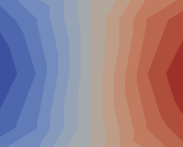
(a) ${\bf{P}}^{L}\rho u^{H}$

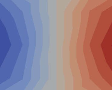
(b) $\hat{\rho u}^{L}$

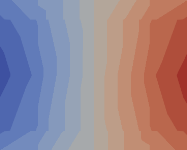
(c) $\rho u^{L}$

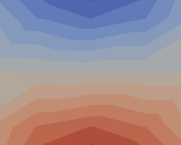
(d) ${\bf{P}}^{L}\rho v^{H}$

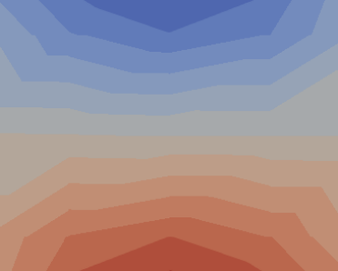
(e) $\hat{\rho v}^{L}$

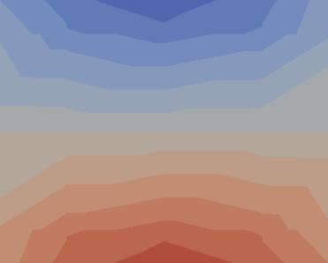
(f) $\rho v^{L}$

Figure 1: 2D Taylor–Green vortex: snapshots of (a) ${\bf{P}}^{L}\rho u^{H}$, (b) $\hat{\rho u}^{L}$, (c) $\rho u^{L}$, (d) ${\bf{P}}^{L}\rho v^{H}$, (e) $\hat{\rho v}^{L}$, and (f) $\rho v^{L}$ with $k_{w}=5$ and $m=1$ at $t=1$.

We further perform a sensitivity study with respect to $m$ and $k_{w}$, and we plot the relative errors of conservative variables ($\rho$, $\rho{\boldsymbol{\varphi}}$, and $\rho E$) at $t=1$ in Figure 2. Here, $\boldsymbol{\varphi}=(u,v)$. In general, varying $m$ and $k_{w}$ does not show any significant differences in density, momentum, and total energy. The relative errors of $\rho$ and $\rho E$ are within $\mathcal{O}(10^{-4})$ and those of $\rho\boldsymbol{\varphi}$ within $\mathcal{O}(10^{-2})$. The minimum and the maximum of the relative errors are $4.7\times 10^{-4}$ and $8.4\times 10^{-4}$ for the density; $1.4\times 10^{-2}$ and $3.2\times 10^{-2}$ for the momentum; and $3.1\times 10^{-4}$ and $4.9\times 10^{-4}$ for the total energy.

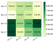
(a) $\rho$

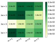
(b) $\rho\varphi$

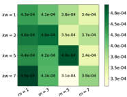
(c) $\rho E$

Figure 2: 2D Taylor–Green vortex: relative errors of (a) $\rho$, (b) $\rho\boldsymbol{\varphi}$, and (c) $\rho E$ with respect to kernel width $k_{w}$ and marching steps $m$.

Since the errors of the momentum are two orders of magnitude larger than the density and the total energy counterparts, we examine the error histories of the conservative variables with $(k_{w},m)=(5,1)$ (which gives the minimum error in the momentum) in Figure 3. The errors of the augmented solution $\hat{\mathbf{{u}}}^{L}$ are smaller than those of the low-order solution $\mathbf{{u}}^{L}$ for $t\in[0,1]$. The errors of $\rho^{L}$ and $\rho{\boldsymbol{\varphi}}^{L}$ are three times bigger than those of $\hat{\rho}^{L}$ and $\hat{\rho\boldsymbol{\varphi}}^{L}$ at $t=1$. Similarly, the error of $\rho E^{L}$ is four times higher than $\hat{\rho E}$ counterpart.

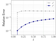
(a) $\rho$

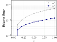
(b) $\rho\boldsymbol{\varphi}$

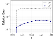
(c) $\rho E$

Figure 3: 2D Taylor–Green vortex: error histories of (a) $\rho$, (b) $\rho\boldsymbol{\varphi}$, and (c) $\rho E$ with $k_{w}=5$ and $m=1$.

4.1.2 Three-dimensional vortex

Next, we consider the three-dimensional Taylor–Green vortex. We integrate the high-order model for third-order ERK with $\triangle t=10^{-3}$ over the mesh of $10\times 10\times 10$ elements (${N_{\text{el}}}=10^{3}$) and the eighth-order polynomial ($N=8$). Figure 4 shows the evolution of the vortices at $t=\left\{0,10,20\right\}$ for $Re=1600$. To visualize the coherent vortical structures in the flow field, we plot Q-criterion isosurfaces with $0.02$, which are colored by the z-component of the vorticity from $-1$ to $1$. The smooth initial vortices are stretched, twisted, and split because of the high Reynolds number, creating turbulent motion. We observe in Figure 5 that the small-scale vortices are generated with increasing Reynolds number .

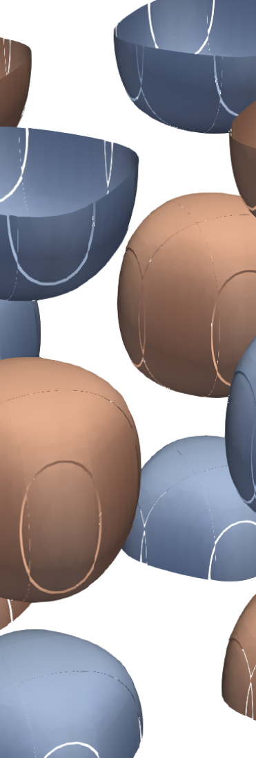
(a) $t=0$

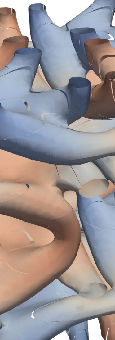
(b) $t=10$

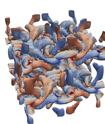
(c) $t=20$

Figure 4: 3D Taylor–Green vortex: Q-criterion isosurfaces for $Re=1600$ with $10^{3}$ elements and $N=8$ at (a) $t=0$, (b) $t=10$, and (c) $t=20$. The isosurfaces are colored by the z-component of the vorticity from $-1$ to $1$.

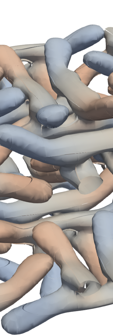
(a) $Re=200$

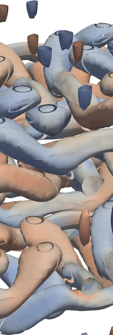
(b) $Re=400$

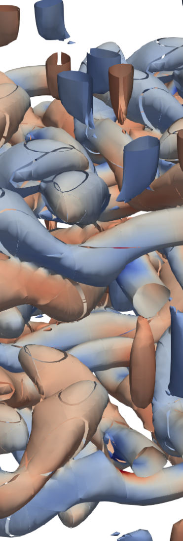
(c) $Re=800$

Figure 5: 3D Taylor–Green vortex: Q-criterion isosurfaces for (a) $Re=200$, (b) $Re=400$, and (c) $Re=800$ with $N=8$ and $10\times 10\times 10$ elements at $t=20$.

Based on this observation, we consider 12 datasets with the starting time $t_{1}\in\left\{0,7,14\right\}$ at $Re\in\left\{100,200,400,1600\right\}$. Similar to the two-dimensional case, we integrate the high-order model with the third-order ERK scheme and the time step size of $10^{-3}$ for one time unit $t\in[t_{1},t_{1}+1]$ over the mesh of the sixth-order polynomial ($N=6$) and $20\times 20\times 20$ (${N_{\text{el}}}=8000$) elements. We use the projection matrix ${\bf{P}}^{L}$ in (5) to obtain the filtered data, and we split the time series of ${{\bf{P}}^{L}}\mathbf{{u}}^{H}$ into the training data for $t=[t_{1},t_{1}+\frac{3}{4}]$ and the test data for $t=[t_{1}+\frac{3}{4},t_{1}+1]$. We train 12 neural network source terms with each dataset. For training a neural network source term, we randomly select two batch instances of ${{\bf{P}}^{L}}\mathbf{{u}}^{H}$ in the training data and integrate (24) for $m$ time steps by using the fifth-order ERK method [62] with ${\triangle t}=10^{-2}$ over the mesh with the first-order $p=1$ polynomial and $20\times 20\times 20$ elements. In a hexahedral element, the eight nodal points (located at vertices) are used for the first-order discontinuous Galerkin methods. Thus, the degrees of freedom of the input and the output layers in (26) are $n_{0}=40\times k_{w}^{3}$ and $n_{D}=40$, respectively. We take the neural network architecture as $\left\{n_{0},64,32,64,n_{D}\right\}$ and train it by using the AdaBelief [63] optimizer with a learning rate of $10^{-3}$ and $1,000$ epochs. The simulation with the same third-order ERK method in different regimes and $Re$ numbers is discussed below.

4.1.3 Results for various time frames at $Re=\left\{100,200,400,1600\right\}$

Figure 6 shows the relative error histories of the density, momentum, and total energy for $Re=100$ with $k_{w}=5$ and $m=11$. Since this flow is in an incompressible regime $M<0.3$, the fluctuation of the density and the total energy is small. Thus the momentum error is two orders of magnitude larger than that of the density and the total energy. In general, the augmented solution (blue solid line) has smaller relative error than the low-order counterpart (grey dash-dot line). Since the flow starts with smoothed profiles, the difference between the low-order and the augmented solutions is small for $t\in[0,1]$. All of the filtered, augmented, and low-order solutions are similar to each other at $t=1$, as shown in Figure 7. As flow evolves, however, the augmented solution shows enhanced accuracy compared with the low-order solution. The momentum error for augmented solutions at $t=8$ and $t=15$ is two times smaller than for the low-order counterpart in Figure 6(b). We see the remarkable improvements in the snapshots at $t=8$ and $t=15$ in Figure 8 and Figure 9, respectively. The augmented solution successfully recovers the vortical structures, whereas the low-order solution quickly loses the vortices because of the numerical dissipation associated with the low-order solver in the viscous-dominated flows.

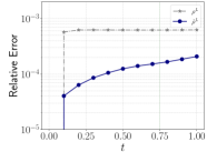
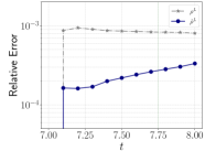
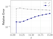
(a) $\rho$

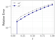
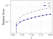
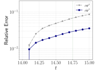
(b) $\rho\boldsymbol{\varphi}$

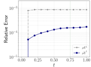
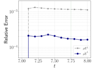
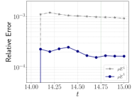
(c) $\rho E$

Figure 6: 3D Taylor–Green vortex: error histories of (a) $\rho$, (b) $\rho\boldsymbol{\varphi}$, and (c) $\rho E$ for $Re=100$ with $k_{w}=1$ and $m=11$.

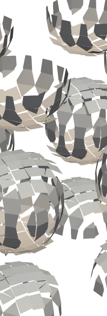
(a) Filtered

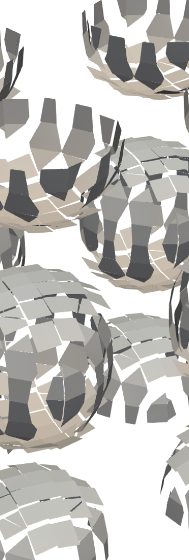
(b) Augmented

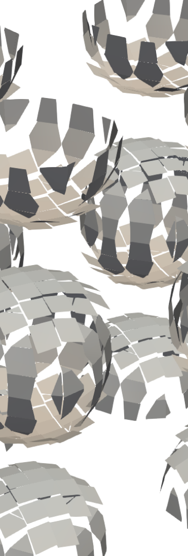
(c) Low-order

Figure 7: 3D Taylor–Green vortex: Q-criterion isosurfaces for $Re=100$ for (a) filtered solution, (b) augmented solution, and (c) low-order solution at $t=1$. The isosurfaces are colored by the z-component of the velocity from $-0.1$ to $0.1$.

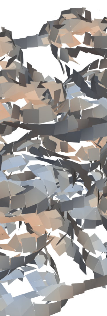
(a) Filtered

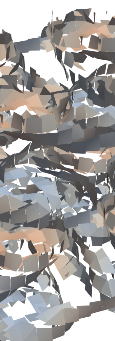
(b) Augmented

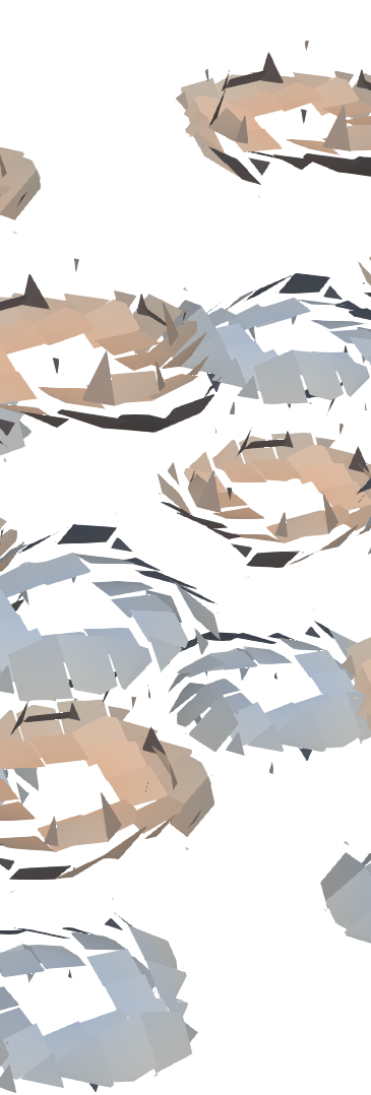
(c) Low-order

Figure 8: 3D Taylor–Green vortex: Q-criterion isosurfaces for $Re=100$ for (a) filtered solution, (b) augmented solution, and (c) low-order solution at $t=8$. The isosurfaces are colored by the z-component of the velocity from $-0.1$ to $0.1$.

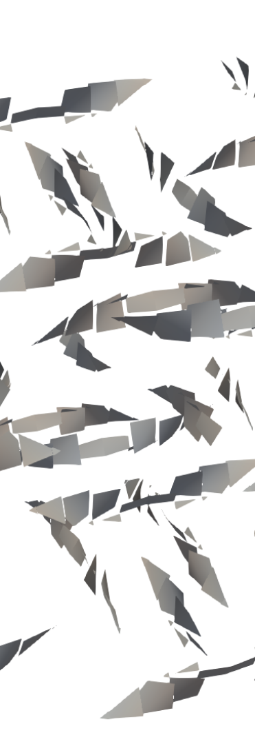
(a) Filtered

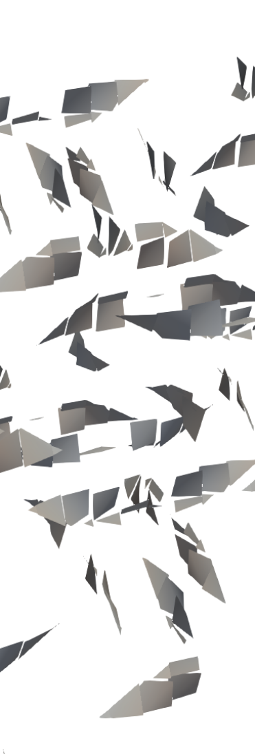
(b) Augmented

(c) Low-order

Figure 9: 3D Taylor–Green vortex: Q-criterion isosurfaces for $Re=100$ for (a) filtered solution, (b) augmented solution, and (c) low-order solution at $t=15$. The isosurfaces are colored by the z-component of the velocity from $-0.1$ to $0.1$.

We plot the relative error histories of the density, momentum, and total energy for $Re=\left\{200,400,1600\right\}$ in Figure 10, Figure 11, and Figure 12, respectively. We note that the accuracy of the augmented solutions highly depends on the hyperparameters such as the kernel width $k_{w}$ and the number of steps $m$. After conducting a sensitivity study with respect to $k_{w}$ and $m$, we choose the best kernel width and the number of steps for each Reynolds number: $k_{w}=1$ and $m=11$ for $Re=200$, $Re=400$, and $Re=1600$. For all the cases with $Re=\left\{200,400,1600\right\}$, the momentum error dominates over the density and the total energy counterparts, similar to the case with $Re=100$. For the low-order solution (grey dash-dot line), the relative momentum error grows as the Reynolds number rises. For example, at $t=15$, the momentum errors of the low-order solution are $1.4\times 10^{-1}$ with $Re=200$ and $3.0\times 10^{-1}$ with $Re=1600$. In comparison with the low-order solution, the augmented solution (blue solid line) has less relative error overall. At $t=8$, the augmented solutions have almost two times smaller momentum errors than do the low-order solutions for $Re=\left\{200,400,1600\right\}$. At $t=15$, the momentum errors of the augmented solution are $6.3\times 10^{-2}$, $1.1\times 10^{-1}$, and $2.0\times 10^{-1}$ for $Re=200$, $Re=400$, and $Re=1600$, which are $2.3$, $2.0$, and $1.5$ times smaller than the low-order counterparts, respectively.

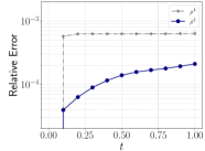
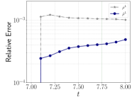
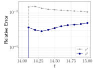
(a) $\rho$

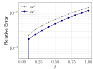
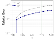
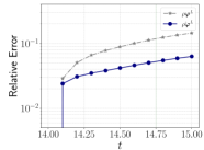
(b) $\rho\boldsymbol{\varphi}$

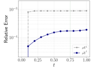
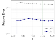
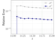
(c) $\rho E$

Figure 10: 3D Taylor–Green vortex: error histories of (a) $\rho$, (b) $\rho\boldsymbol{\varphi}$, and (c) $\rho E$ for $Re=200$ with $k_{w}=1$ and $m=11$.

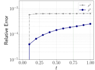
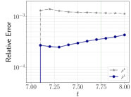
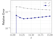
(a) $\rho$

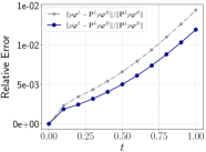
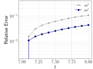
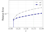
(b) $\rho\boldsymbol{\varphi}$

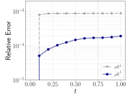
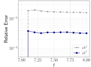
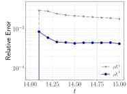
(c) $\rho E$

Figure 11: 3D Taylor–Green vortex: error histories of (a) $\rho$, (b) $\rho\boldsymbol{\varphi}$, and (c) $\rho E$ for $Re=400$ with $k_{w}=1$ and $m=11$.

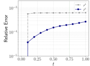
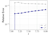
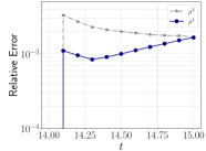
(a) $\rho$

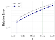
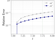
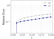
(b) $\rho\boldsymbol{\varphi}$

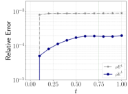
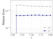
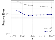
(c) $\rho E$

Figure 12: 3D Taylor–Green vortex: error histories of (a) $\rho$, (b) $\rho\boldsymbol{\varphi}$, and (c) $\rho E$ for $Re=1600$ with $k_{w}=1$ and $m=11$.

Figure 13 and Figure 14 show the snapshots of the filtered, augmented, and low-order solutions for $Re=\left\{200,400,1600\right\}$ at $t=8$ and $t=15$, respectively. With increasing Reynolds number, the flow becomes turbulent, and hence the vortical structures are more prevalent because of the mixing. In both figures, the augmented solutions demonstrate significant improvements at $Re=\left\{200,400,1600\right\}$. Indeed, the neural network source term recovers the misrepresented scales and enhances the accuracy of the low-order approximation.

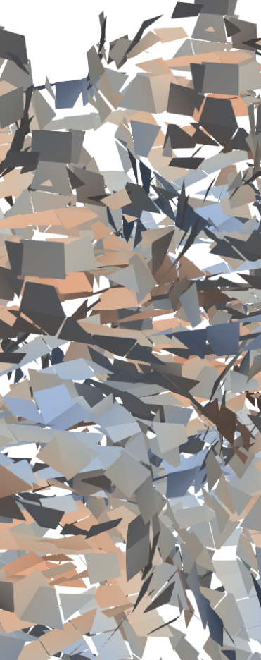
(a) Filtered at $Re=200$

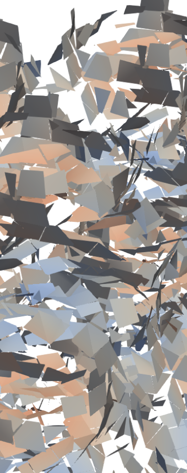
(b) Augmented at $Re=200$

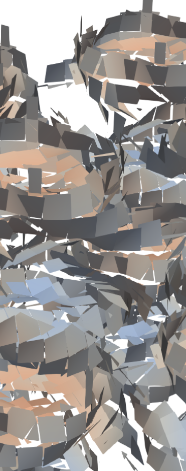
(c) Low-order at $Re=200$

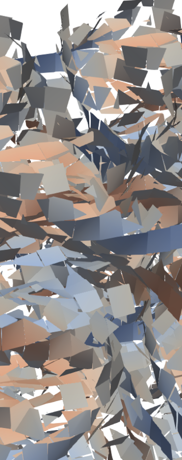
(d) Filtered at $Re=400$

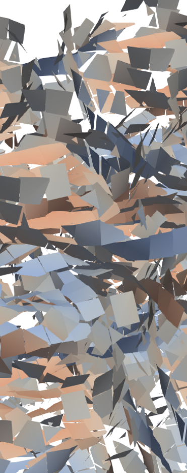
(e) Augmented at $Re=400$

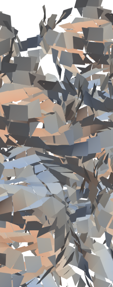
(f) Low-order at $Re=400$

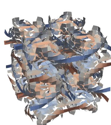
(g) Filtered at $Re=1600$

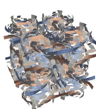
(h) Augmented at $Re=1600$

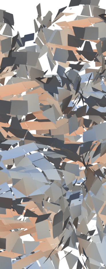
(i) Low-order at $Re=1600$

Figure 13: 3D Taylor–Green vortex: Q-criterion isosurfaces for $Re=\left\{200,400,1600\right\}$ for (a) filtered solution, (b) augmented solution, and (c) low-order solution at $t=8$. The isosurfaces are colored by the z-component of the velocity from $-0.1$ to $0.1$.

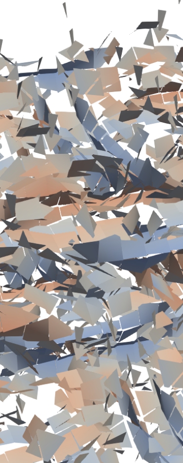
(a) Filtered at $Re=200$

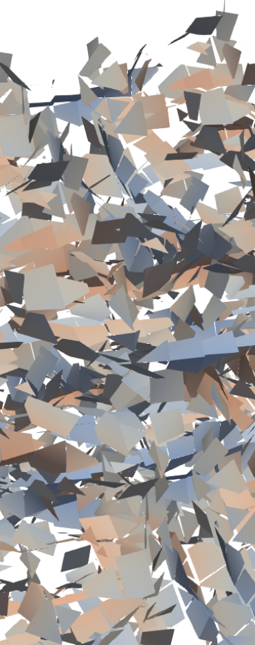
(b) Augmented at $Re=200$

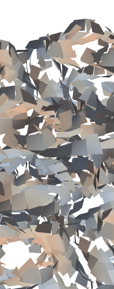
(c) Low-order at $Re=200$

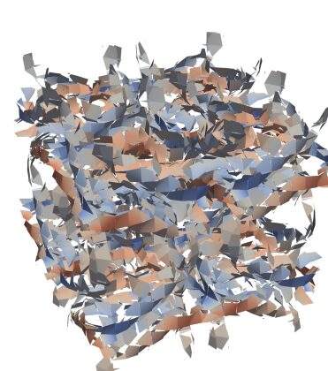
(d) Filtered at $Re=400$

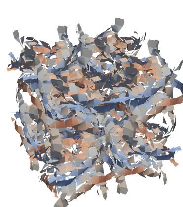
(e) Augmented at $Re=400$

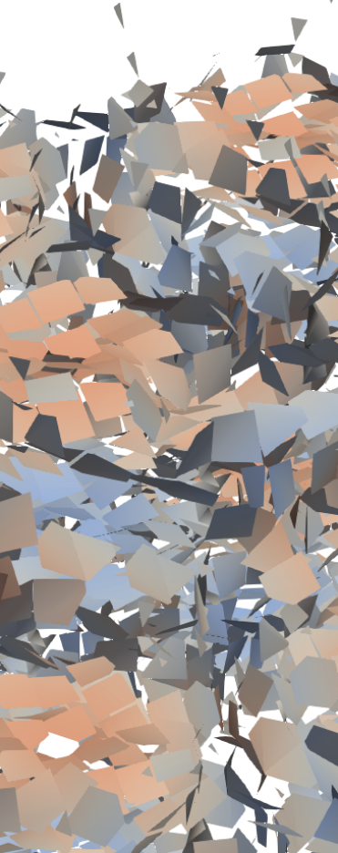
(f) Low-order at $Re=400$

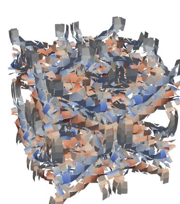
(g) Filtered at $Re=1600$

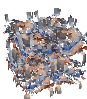
(h) Augmented at $Re=1600$

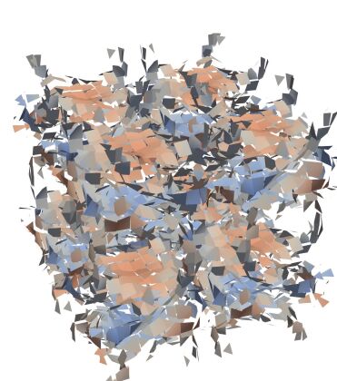
(i) Low-order at $Re=1600$

Figure 14: 3D Taylor–Green vortex: Q-criterion isosurfaces for $Re=\left\{200,400,1600\right\}$ for (a) filtered solution, (b) augmented solution, and (c) low-order solution at $t=15$. The isosurfaces are colored by the z-component of the velocity from $-0.1$ to $0.1$.

4.1.4 Sensitivity test for the kernel width $k_{w}$ and the number of steps $m$

In this subsection we present a sensitivity study of the prediction of the augmented solution with respect to the kernel width $k_{w}\in\left\{1,3,5\right\}$ and the number of steps $m\in\left\{1,3,7,11\right\}$ for $Re=100$ and $Re=1600$; see Figure 15. Since the momentum error dominates over the density and the total energy counterparts in this example, we show only the momentum errors. We also choose the time interval of $t\in[14,15]$ because the errors are larger than those of $t\in[0,1]$ and $t\in[7,8]$. In general, the relative error decreases with increasing number of steps $m$, except for some cases. For $Re=1600$ and $k_{w}=5$, $m=7$ produces smaller error than $m=11$. Even in these cases, however, $m=11$ (green solid line) shows better accuracy than $m=1$ (red dash-dot line). The best cases are $k_{w}=5,m=11$ at $Re=100$ and $k_{w}=1,m=11$ at $Re=1600$. Turbulent flows appear to perform better with single-kernel width for training, but laminar flows appear to perform better with multiple-kernel width.

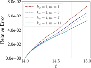
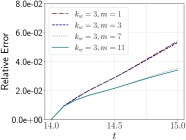
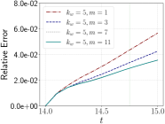
(a) $Re=100$

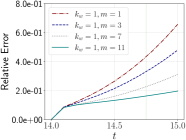
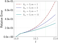
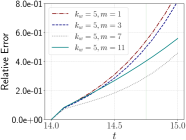
(b) $Re=1600$

Figure 15: 3D Taylor–Green vortex: error histories of $\hat{\rho\boldsymbol{\varphi}}$ for $Re\in\left\{100,1600\right\}$ with respect to the number of steps $m$.

4.1.5 Computational cost

We train the neural network source term and measure the wall-clock times of the prediction of $\hat{\mathbf{{u}}}^{L}$, $\mathbf{{u}}^{L}$, and $\mathbf{{u}}^{H}$ on ThetaGPU at the Argonne Leadership Computing Facility using a single NVIDIA DGX A100.

For the predictions, we choose the stable time step size $\triangle t$ such that doubling the time step size leads to a blowup. The stable time step sizes are $\triangle t^{H}=10^{-3}$ for high-order solution and $\triangle t^{L}=2\times 10^{-2}$ for low-order and augmented solutions. We make the predictions five times from $t=14$ to $t=15$ and report the average wall-clock times in Table 1 for $Re=100$ and in Table 2 for $Re=1600$. We denote $\hat{\mathbf{{u}}}^{L}$ with $k_{w}=1$, $\hat{\mathbf{{u}}}^{L}$ with $k_{w}=3$, and $\hat{\mathbf{{u}}}^{L}$ with $k_{w}=5$ by $\hat{\mathbf{{u}}}^{L}(k_{w}=1)$, $\hat{\mathbf{{u}}}^{L}(k_{w}=3)$, and $\hat{\mathbf{{u}}}^{L}(k_{w}=5)$ for brevity. We measure the wall clock twice since JAX has a just-in-time (JIT) compilation. The reason for doing this is that when a function is called for the first time in JAX, it is compiled and the resulting code is cached. As a result, the subsequent run times after the first are significantly faster. We compute JIT compiling time by subtracting the second wall-clock time from the first wall-clock time.

For the JIT compiling time, $\hat{\mathbf{{u}}}^{H}$ takes about $2.5$ times more time than the others, but $\mathbf{{u}}^{L}$, $\hat{\mathbf{{u}}}^{L}(k_{w}=1)$, $\hat{\mathbf{{u}}}^{L}(k_{w}=3)$, and $\hat{\mathbf{{u}}}^{L}(k_{w}=5)$ are comparable to each another. For the second run with a cached code, the wall clock of $\hat{\mathbf{{u}}}^{L}(k_{w}=1)$ is comparable to that of the low-order solution $\mathbf{{u}}^{L}$. With increasing kernel width $k_{w}$, the wall clock of $\hat{\mathbf{{u}}}^{L}$ grows. The wall clock of $\hat{\mathbf{{u}}}^{L}(k_{w}=3)$ is $14\%$ larger than that of $\hat{\mathbf{{u}}}^{L}(k_{w}=1)$. The wall clock of $\hat{\mathbf{{u}}}^{L}(k_{w}=5)$ is $48\%$ larger than that of $\hat{\mathbf{{u}}}^{L}(k_{w}=1)$. This is expected because the input size of the neural network source term increases with increasing the kernel width. The wall clock of the low-order solution $\mathbf{{u}}^{L}$ is $620$ times smaller than that of the high-order solution $\mathbf{{u}}^{H}$. The augmented solutions $\hat{\mathbf{{u}}}^{L}$ with $k_{w}=1$, $k_{w}=3$, and $k_{w}=5$ are about $620$, $543$, and $425$ times faster than the high-order solution $\mathbf{{u}}^{H}$, respectively. Indeed, compared with the high-order solution, the augmented solutions speed up two orders of magnitude. These results provide a significant speedup boost over the one-dimensional cases in [30], where augmenting the neural network source is $3$ and $19$ times more economical for the one-dimensional convection-diffusion model and the one-dimensional viscous Burgers’ model.

Table 1: 3D Taylor–Green vortex: wall-clock time for the predictions of $\mathbf{{u}}^{H}$, $\mathbf{{u}}^{L}$, and $\hat{\mathbf{{u}}}^{L}$ from $t=14$ to $t=15$ at $Re=100$.

	${\triangle t}$	JIT Compile wc [$s$]	Simulation wc [$s$]
$\mathbf{{u}}^{H}$	$0.001$	47.0	217
$\mathbf{{u}}^{L}$	$0.02$	17.72	0.35
$\hat{\mathbf{{u}}}^{L}(k_{w}=1)$	$0.02$	18.05	0.35
$\hat{\mathbf{{u}}}^{L}(k_{w}=3)$	$0.02$	18.04	0.40
$\hat{\mathbf{{u}}}^{L}(k_{w}=5)$	$0.02$	18.35	0.51

Table 2: 3D Taylor–Green vortex: wall-clock time for the predictions of $\mathbf{{u}}^{H}$, $\mathbf{{u}}^{L}$, and $\hat{\mathbf{{u}}}^{L}$ from $t=14$ to $t=15$ at $Re=1600$.

	${\triangle t}$	JIT Compile wc [$s$]	Simulation wc [$s$]
$\mathbf{{u}}^{H}$	$0.001$	47.4	217
$\mathbf{{u}}^{L}$	$0.02$	17.83	0.33
$\hat{\mathbf{{u}}}^{L}(k_{w}=1)$	$0.02$	18.56	0.36
$\hat{\mathbf{{u}}}^{L}(k_{w}=3)$	$0.02$	18.11	0.39
$\hat{\mathbf{{u}}}^{L}(k_{w}=5)$	$0.02$	18.53	0.49

4.1.6 Comparison with the discrete corrective forcing approach

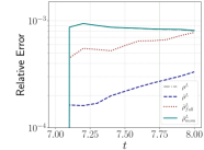
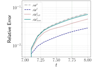
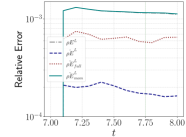
(a) $Re=100$

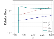
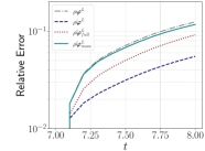
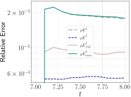
(b) $Re=1600$

Figure 16: 3D Taylor-Green vortex: error histories of (a) $\rho$, (b) $\rho{\boldsymbol{\varphi}}$, and (c) $\rho E$ for $Re=1600$ with discrete forcing approaches.

Compared with the discrete corrective forcing approach [29, 7], our method involves learning a continuous corrective forcing term. Consequently, it can seamlessly adapt its time step size during both training and prediction phase. In our previous study [30], we conducted numerical experiments demonstrating that our proposed approach exhibited robustness when the time step size varied for the one-dimensional convection-diffusion equation. In particular, our proposed approach outperformed the discrete corrective forcing approach in terms of accuracy, except when evaluated with the time step size designed especially for the discrete corrective forcing approach. However, in the case of the three-dimensional Taylor–Green vortex example, both the discrete and continuous corrective forcing approaches showed little sensitivity to variations in time step size. The reason is that spatial discretization errors were dominant in this example. Therefore, we only report the relative error histories for both methods using the time step size that was used for training the discrete forcing term.

We construct the discrete corrective forcing term $\tilde{{\bf S}}_{\theta}$ for compressible Navier–Stokes equations as follows. First we generate the filtered high-order solution with the time step size ${\triangle t}^{H}$. Second we create the discrete corrective forcing data, $\tilde{{\bf S}}_{\theta,n}$ for $n=0,\cdots,N_{t}$. Here, the $k$th component of $\tilde{{\bf S}}_{\theta,n}$ is obtained by $\left(\tilde{S}_{k}\right)_{\theta,n}=\frac{{\bf{P}}^{L}\left(u^{H}_{k}\right)_{n+1}-\left(u^{L}_{k}\right)_{n+1}}{{\triangle t}^{L}}$, where $u^{H}_{k}$ and ${u}^{L}_{k}$ represent the $k$th conservative variables of $\mathbf{{u}}^{H}$ and $\mathbf{{u}}^{L}$, respectively. We take ${\triangle t}^{L}=10\times{\triangle t}^{H}$. Then we consider two types of discrete forcing terms: $\tilde{{\bf S}}_{\theta,mom}$ and $\tilde{{\bf S}}_{\theta,full}$. The former corrects the momentum equations, $\tilde{{\bf S}}_{\theta,mom}=\left(0,\tilde{{\bf S}}_{\rho\boldsymbol{\varphi}},0\right)^{T}$, while the latter deals with the full equations, $\tilde{{\bf S}}_{\theta,full}=\left(\tilde{S}_{\rho},\tilde{{\bf S}}_{\rho\boldsymbol{\varphi}},\tilde{S}_{\rho E}\right)^{T}$. We denote the discretely corrected solutions through $\tilde{{\bf S}}_{\theta,mom}$ and $\tilde{{\bf S}}_{\theta,full}$ by $\tilde{\mathbf{{u}}}_{mom}^{L}$ and $\tilde{\mathbf{{u}}}_{full}^{L}$, respectively. Next we construct two nonlinear maps from the input feature of $\left({\bf{P}}^{L}\rho^{H},{\bf{P}}^{L}\rho u^{H},{\bf{P}}^{L}\rho v^{H},{\bf{P}}^{L}\rho w^{H},{\bf{P}}^{L}\rho E^{H}\right)^{T}$ to the output features of $\tilde{{\bf S}}_{\theta,mom}$ and $\tilde{{\bf S}}_{\theta,full}$ by using a feed-forward neural network. For $\tilde{{\bf S}}_{\theta,mom}$ and $\tilde{{\bf S}}_{\theta,full}$, we take the dimension of the neural network architectures as $\left\{40,64,32,64,24\right\}$ and $\left\{40,64,32,64,40\right\}$, respectively. Both discrete corrective forcing terms are again trained by using the AdaBelief [63] optimizer with a learning rate of $10^{-3}$, $2$ batches and $1000$ epochs.

Figure 16 shows the relative errors of the density, momentum, and total energy of the low-order (first-order) solution ($\mathbf{{u}}^{L}$), the augmented solution ($\hat{\mathbf{{u}}}^{L}$), and the discretely corrected solutions ($\tilde{\mathbf{{u}}}^{L}_{mom}$ and $\tilde{\mathbf{{u}}}^{L}_{full}$) for $t\in[7,8]$ at $Re=\left\{100,1600\right\}$. In general, our approach (the continuous corrective forcing method) outperforms the discrete forcing approach for the density, the momentum, and the total energy. For the density, $\hat{\rho u}^{L}$ has two times lower error than both $\tilde{\rho u}^{L}_{mom}$ and $\tilde{\rho u}^{L}_{full}$ at $t=8$. For the momentum, $\hat{\rho\boldsymbol{\varphi}}^{L}$ has an error level that is half of $\tilde{\rho\boldsymbol{\varphi}}^{L}_{mom}$, and the error level of $\hat{\rho\boldsymbol{\varphi}}^{L}$ is about $1.5$ times lower than that of $\tilde{\rho\boldsymbol{\varphi}}^{L}_{full}$ at $t=8$. For the total energy, $\hat{\rho E}^{L}$ has four times less error than $\tilde{\rho E}^{L}_{full}$ and $6.9$ times less error than $\tilde{\rho E}^{L}_{mom}$ at $Re=100$, whereas $\hat{\rho E}^{L}$ has $1.6$ times less error than $\tilde{\rho E}^{L}_{full}$ and $3.2$ times less error than $\tilde{\rho E}^{L}_{mom}$ at $Re=1600$. When we compare the two discrete forcing approaches, $\tilde{{\bf S}}_{\theta,full}$ provides more accurate predictions than $\tilde{{\bf S}}_{\theta,mom}$. $\tilde{\rho\boldsymbol{\varphi}}^{L}_{mom}$ has $1.7$ and two times larger error than $\tilde{\rho\boldsymbol{\varphi}}^{L}_{full}$ at $Re=100$ and $Re=1600$, respectively. $\tilde{\rho\boldsymbol{\varphi}}^{L}_{mom}$ at $Re=100$ has $1.7$ times larger error than $\tilde{\rho\boldsymbol{\varphi}}^{L}_{full}$; and at $Re=1600$, its error is twice as large as that of $\tilde{\rho\boldsymbol{\varphi}}^{L}_{full}$.

4.1.7 Comparison with the second- and the third-order DG approximations

(a) $\rho u$

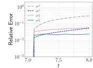
(b) $\rho v$

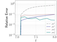
(c) $\rho w$

Figure 17: 3D Taylor–Green vortex: error histories of (a) $\rho u$, (b) $\rho v$, and (c) $\rho w$ at $Re=1600$ for $\mathbf{{u}}^{L}$, $\hat{\mathbf{{u}}}^{L}$, $\mathbf{{u}}^{L}_{2}$, and $\mathbf{{u}}^{L}_{3}$.

Up to this point, we numerically showed that the augmented DG approximation has better accuracy than the low-order DG approximation. Now we examine how much our approach improves the accuracy of the low-order DG approximation by comparing the second- and the third-order DG approximations. We choose the mesh of the eighth-order polynomial ($N=8$) and $8\times 8\times 8$ (${N_{\text{el}}}=512$) elements. We integrate the high-order model with the third-order ERK scheme and the time step size of $10^{-3}$ for one time unit $t\in[7,8]$ at $Re=1600$. We project the eighth-order solution to the first-order space to obtain the filtered data. Then we divide its time series into both the training data for $t=[7,7.75]$ and the test data for $t=[7.75,8]$. We choose the dimension of the neural network source as $\left\{40,128,128,128,40\right\}$. We take the AdaBelief [63] optimizer with a learning rate of $10^{-3}$ and $2,000$ epochs. We denote the second- and the third-order DG approximations by $\mathbf{{u}}_{2}$ and $\mathbf{{u}}_{3}$, respectively. We let $\mathbf{{u}}^{L}_{2}$ and $\mathbf{{u}}^{L}_{3}$ respectively be the projected solutions of $\mathbf{{u}}_{2}$ and $\mathbf{{u}}_{3}$ onto the first-order polynomial space on each element. For the initial conditions of $\mathbf{{u}}_{2}$ and $\mathbf{{u}}_{3}$, we interpolate the initial profile of $\mathbf{{u}}^{L}$ to the second- and the third-order polynomial spaces. We integrate $\mathbf{{u}}^{L}$, $\hat{\mathbf{{u}}}^{L}$, $\mathbf{{u}}_{2}$, and $\mathbf{{u}}_{3}$ with ${\triangle t}=10^{-3}$ for $t=[7,8]$. We measure the relative $L^{2}$ errors for $\mathbf{{u}}^{L}$, $\hat{\mathbf{{u}}}^{L}$, $\mathbf{{u}}_{2}^{L}$, and $\mathbf{{u}}^{L}_{3}$ by taking ${\bf{P}}^{L}\mathbf{{u}}^{H}$ as the ground truth. Since the momentum error is dominant over the density and the total energy counterparts, we plot the relative errors of the momentum variables ($\rho u$, $\rho v$, and $\rho w$) in Figure 17. For $t=[7,7.25]$, the augmented DG approximations of $\hat{\rho u}^{L}$, $\hat{\rho v}^{L}$, and $\hat{\rho w}^{L}$ show better accuracy than the others. When $t=7.25$, the third-order DG approximations catch up with the accuracy levels of $\hat{\rho u}^{L}$, $\hat{\rho v}^{L}$, and $\hat{\rho w}^{L}$. After $t=7.25$, the relative errors of ${\rho u}^{L}_{3}$, ${\rho v}^{L}_{3}$, and ${\rho w}^{L}_{3}$ become smaller than those of $\hat{\rho u}^{L}$, $\hat{\rho v}^{L}$, and $\hat{\rho w}^{L}$. For $t=[7.25,8]$, the augmented DG approximations of $\hat{\rho u}^{L}$, $\hat{\rho v}^{L}$, and $\hat{\rho w}^{L}$ have still higher accuracy than the first- and the second-order DG approximation counterparts. At $t=8.0$, the relative errors of the augmented DG approximations become comparable to those of ${\rho u}^{L}_{2}$, ${\rho v}^{L}_{2}$, and ${\rho w}^{L}_{2}$.

5 Conclusions

In our previous work [30] we presented a methodology for learning subgrid-scale models based on neural ordinary differential equations, where the one-dimensional convection-diffusion equation and viscous Burgers’ equation are discussed in the context of DG methods. In this work we extend our approach to multidimensional compressible Navier–Stokes equations. Our goal is to learn the unresolved scales of the low-order DG solver at a continuous level by utilizing high-order DG simulation data and NODEs. To achieve this goal, we first create a differentiable DG model on a structured mesh for compressible Navier–Stokes equations. Then, we introduce a neural network source term to the spatially discretized DG formulation. This is a hybrid model that combines traditional numerical methods with machine learning, leveraging the precision of numerical methods and the efficiency of machine learning techniques. We devise a local network source function, which is composed of a $D$-depth feed-forward neural network, slides over the low-order solutions of all the elements, and produces a local source approximation for each element. Next, we train the neural network parameters through NODEs. Then, we predict the augmented solution with the neural network augmented DG system with standard time-stepping methods such as explicit Runge–Kutta methods. The suggested method learns the continuous source operator for low-order DG solvers to account for the misrepresented scales, predicting a solution with a larger time step size than that of the high-order DG solvers. This can significantly accelerate the filtered high-order simulation.

We demonstrate the proposed methodology through multidimensional Taylor–Green vortex examples. We consider stable vortices for $t\in[0,1]$ at $Re=100$ in the two-dimensional case and various flow regimes with different Reynolds numbers $Re=\left\{100,200,400,1600\right\}$ and times $t\in\left\{[0,1],[7,8],[14,15]\right\}$ in the three-dimensional case. Augmenting a neural network source term indeed enhances the low-order approximation’s accuracy. In both the two-dimensional and the three-dimensional examples, the augmented solution shows lower error histories of the density, momentum, and total energy than does the low-order solution. In particular, we observe that the augmented solution recovers the misrepresented scales from the low-order solutions, as shown in the snapshots at $t=8$ and $t=15$. We also conducted the sensitivity study with respect to the kernel width $k_{w}$ and the number of steps $m$. We found that the momentum error tends to decrease as the number of steps increases. It seems that a single local kernel width works better for turbulent flows than for laminar flows, whereas slightly increasing the kernel width is more appropriate for laminar flows than for turbulent flows. Compared to the second- and the third-order approximation, we numerically observed that the augmented solution (first-order) has comparable error levels between the second- and the third-order approximation for $Re=1600$.

We reported the wall-clock times for the low-order approximation, the augmented low-order approximation, and the high-order approximation. The high-order approximation is $620$ times more expensive than the low-order approximation. Compared with the high-order approximation, the augmented solution is two orders of magnitude faster. With the single-kernel width, the augmented approximation is $620$ times more economical than the high-order approximation.

Our approach can be viewed as an extension of the discrete corrective forcing approach. We demonstrated that the discrete corrective forcing approach relies on the temporal discretization of a sequential operator-splitting step, whereas our proposed method is founded on the continuous form of ordinary differential equations without any operator-splitting step. Consequently, our approach learns the continuous source dynamics, enabling it to adapt to variable time steps during training and prediction, without introducing operator-splitting errors. Indeed, we numerically demonstrate that our proposed approach performs better than the discrete corrective forcing approach in terms of accuracy for the case of $Re=100$ and $Re=1600$.

Current work successfully demonstrates the potential applicability of employing a neural network source function in conjunction with neural ordinary differential equations for multidimensional compressible Navier–Stokes equations. Augmenting the neural network source function not only improves the accuracy of the low-order DG approximation but also significantly speeds up the filtered high-order simulation with a certain degree of precision. Hybrid models including our approach have an opportunity to become widely adopted simulation-based tools in the future, thanks to their speed, accuracy, and efficiency. They hold great promise for applications in turbulent fluid dynamics, climate modeling, and weather simulations. Furthermore, we believe that our approach has a benefit for parallel training neural network parameters because DG approaches provide favorable parallel performance and the neural network source function is local. That is, our approach is independent of the problem size. We will investigate this aspect in future work.

Our current approach does, however, have limitations. We did not explore complex problems, for which we may need the global neural network source function instead of the local neural network source function. Also, the DG discretization loses the conservation property by introducing the neural network source term. Moreover, the neural network source function is trained with particular parameters. Therefore, we will explore different neural network architectures that have the potential to alleviate issues with more complex examples.

Appendix A Compressible Navier–Stokes Equations

The homogeneous compressible Navier–Stokes equations in $\Omega$ are described by

$$\frac{\partial{\rho}}{\partial{t}}+\nabla\cdot\left(\rho{\boldsymbol{\varphi}}\right) =0,$$ (29a)

$$\frac{\partial{\rho{\boldsymbol{\varphi}}}}{\partial{t}}+\nabla\cdot\left(\rho{\boldsymbol{\varphi}}\otimes{\boldsymbol{\varphi}}+\mathcal{I}{{p}}\right) =\nabla\cdot\sigma,$$ (29b)

$$\frac{\partial{\rho E}}{\partial{t}}+\nabla\cdot\left(\rho{\boldsymbol{\varphi}}H\right) =\nabla\cdot(\sigma{\boldsymbol{\varphi}})-\nabla\cdot\Pi,$$ (29c)

where $\rho$ is the density $[$\mathrm{kg}\text{\,}{\mathrm{m}}^{-3}$]$; ${\boldsymbol{\varphi}}$ is the velocity vector $[$\mathrm{m}\text{\,}{\mathrm{s}}^{-1}$]$; ${{p}}$ is the pressure $[$\mathrm{N}\text{\,}{\mathrm{m}}^{-2}$]$; $\rho E=\rho e+\frac{1}{2}\rho\|{\boldsymbol{\varphi}}\|^{2}$ is the total energy $[$\mathrm{J}\text{\,}{\mathrm{m}}^{-3}$]$; $e=\frac{{{p}}}{\rho(\gamma-1)}$ is the internal energy $[$\mathrm{J}\text{\,}{\mathrm{kg}}^{-1}$]$; $H=E+\frac{{{p}}}{\rho}=\frac{a^{2}}{\gamma-1}+\frac{1}{2}\|{\boldsymbol{\varphi}}\|^{2}$ is the total specific enthalpy $[$\mathrm{J}\text{\,}{\mathrm{kg}}^{-1}$]$; $\sigma=\mu\left(\nabla{\boldsymbol{\varphi}}+\nabla({\boldsymbol{\varphi}})^{T}-\frac{2}{3}\mathcal{I}\nabla\cdot{\boldsymbol{\varphi}}\right)$ is the viscous stress tensor; $\Pi=-\kappa\nabla T$ is the heat flux; $T_{m}$ is the temperature; $\kappa=\mu~{}c_{p}~{}Pr^{-1}$ is the heat conductivity $[$\mathrm{W}\text{\,}{\mathrm{m}}^{-1}\text{\,}{\mathrm{K}}^{-1}$]$; $\mu$ is the dynamic viscosity $[$\mathrm{Pa}\text{\,}\mathrm{s}$]$; $Pr$ is the Prandtl number; $a=\left(\gamma{{p}}\rho^{-1}\right)^{\frac{1}{2}}$ is the sound speed $[$\mathrm{m}\text{\,}{\mathrm{s}}^{-1}$]$ for an ideal gas; $\gamma=c_{p}c_{v}^{-1}$ is the ratio of the specific heats; and $c_{p}$ and $c_{v}$ are the specific heat capacities at constant pressure and at constant volume $[$\mathrm{J}\text{\,}{\mathrm{kg}}^{-1}\text{\,}{\mathrm{K}}^{-1}$]$, respectively.

By the nondimensionalized variables using the speed of sound as a reference velocity,

$$\rho^{*}=\frac{\rho}{\rho_{\infty}},{{p}}^{*}=\frac{{{p}}}{\rho_{\infty}a_{\infty}^{2}},{\boldsymbol{\varphi}}^{*}=\frac{{\boldsymbol{\varphi}}}{a_{\infty}},x^{*}=\frac{x}{L},t^{*}=\frac{t}{L/a_{\infty}},\mu^{*}=\frac{\mu}{\mu_{\infty}},\text{ and }T^{*}=\frac{T}{T_{\infty}},$$

we rewrite the governing equation (29) as

$$\frac{\partial{\rho^{*}}}{\partial{t^{*}}}+\nabla^{*}\cdot\left(\rho{\boldsymbol{\varphi}}^{*}\right) =0,$$ (30a)

$$\frac{\partial{\rho{\boldsymbol{\varphi}}^{*}}}{\partial{t^{*}}}+\nabla^{*}\cdot\left(\rho{\boldsymbol{\varphi}}^{*}\otimes{\boldsymbol{\varphi}}^{*}+\mathcal{I}{{p}}^{*}\right) =\nabla^{*}\cdot\sigma^{*},$$ (30b)

$$\frac{\partial{\rho E^{*}}}{\partial{t^{*}}}+\nabla^{*}\cdot\left(\rho{\boldsymbol{\varphi}}^{*}H^{*}\right) =\nabla^{*}\cdot(\sigma^{*}{\boldsymbol{\varphi}}^{*})-\nabla^{*}\cdot\Pi^{*},$$ (30c)

where $\sigma^{*}=\tilde{\mu}\left(\nabla^{*}{\boldsymbol{\varphi}}^{*}+\nabla^{*}({\boldsymbol{\varphi}}^{*})^{T}-\frac{2}{3}\mathcal{I}\nabla^{*}\cdot{\boldsymbol{\varphi}}^{*}\right)$, $\Pi^{*}=-\frac{\tilde{c}_{p}\tilde{\mu}}{Pr}\nabla^{*}T^{*}$, $\nabla^{*}=\frac{1}{L}\nabla$, $\tilde{\mu}=\frac{\mu^{*}~{}M_{\infty}}{Re_{\infty}}$, $Re_{\infty}=\frac{\rho_{\infty}u_{\infty}L}{\mu_{\infty}}$, $M_{\infty}=\frac{u_{\infty}}{a_{\infty}}$, and $\tilde{c}_{p}:=\frac{1}{\gamma-1}$. The normalized equation of state for an ideal gas is ${{p}}^{*}=\gamma^{-1}\rho^{*}T^{*}=\rho^{*}e^{*}(\gamma-1)$. Sutherland’s formula is $\mu^{*}=\left(T^{*}\right)^{\frac{3}{2}}\frac{1+\frac{su}{T_{\infty}}}{T^{*}+\frac{su}{T_{\infty}}}$ with $su=110.4~{}$\mathrm{K}$$. In this study, we use the nondimensionalized form (30), and we omit the superscript ($*$).

Government License (will be removed at publication): The submitted manuscript has been created by UChicago Argonne, LLC, Operator of Argonne National Laboratory (“Argonne”). Argonne, a U.S. Department of Energy Office of Science laboratory, is operated under Contract No. DE-AC02-06CH11357. The U.S. Government retains for itself, and others acting on its behalf, a paid-up nonexclusive, irrevocable worldwide license in said article to reproduce, prepare derivative works, distribute copies to the public, and perform publicly and display publicly, by or on behalf of the Government. The Department of Energy will provide public access to these results of federally sponsored research in accordance with the DOE Public Access Plan. http://energy.gov/downloads/doe-public-access-plan.

References

- [1] W. H. Reed, T. R. Hill, Triangular mesh methods for the neutron transport equation, Los Alamos Report LA-UR-73-479.
- [2] B. Cockburn, G. E. Karniadakis, C.-W. Shu, The development of discontinuous Galerkin methods, in: Discontinuous Galerkin methods: theory, computation and applications, Springer, 2000, pp. 3–50.
- [3] D. N. Arnold, F. Brezzi, B. Cockburn, L. D. Marini, Unified analysis of discontinuous Galerkin methods for elliptic problems, SIAM Journal on Numerical Analysis 39 (5) (2002) 1749–1779.
- [4] T. Bui-Thanh, O. Ghattas, Analysis of an hp-nonconforming discontinuous Galerkin spectral element method for wave propagation, SIAM Journal on Numerical Analysis 50 (3) (2012) 1801–1826.
- [5] J. Rudi, A. C. I. Malossi, T. Isaac, G. Stadler, M. Gurnis, P. W. Staar, Y. Ineichen, C. Bekas, A. Curioni, O. Ghattas, An extreme-scale implicit solver for complex PDEs: highly heterogeneous flow in earth’s mantle, in: Proceedings of the International Conference for High Performance Computing, Networking, Storage and Analysis, 2015, pp. 1–12.
- [6] S. Kang, T. Bui-Thanh, A scalable exponential-DG approach for nonlinear conservation laws: With application to Burger and Euler equations, Computer Methods in Applied Mechanics and Engineering 385 (2021) 114031.
- [7] F. M. de Lara, E. Ferrer, Accelerating high order discontinuous Galerkin solvers using neural networks: 3D compressible Navier-Stokes equations, Journal of Computational Physics (2023) 112253.
- [8] P. Sagaut, M. Germano, On the filtering paradigm for LES of flows with discontinuities, Journal of Turbulence (6) (2005) N23.
- [9] A. D. Beck, D. G. Flad, C. Tonhäuser, G. Gassner, C.-D. Munz, On the influence of polynomial de-aliasing on subgrid scale models, Flow, Turbulence and Combustion 97 (2016) 475–511.
- [10] J. Smagorinsky, General circulation experiments with the primitive equations: I. the basic experiment, Monthly Weather Review 91 (3) (1963) 99–164.
- [11] M. Germano, U. Piomelli, P. Moin, W. H. Cabot, A dynamic subgrid-scale eddy viscosity model, Physics of Fluids A: Fluid Dynamics 3 (7) (1991) 1760–1765.
- [12] S. Collis, The DG/VMS method for unified turbulence simulation, in: 32nd AIAA Fluid Dynamics Conference and Exhibit, 2002, p. 3124.
- [13] K. Sengupta, F. Mashayek, G. Jacobs, Large-eddy simulation using a discontinuous Galerkin spectral element method, in: 45th AIAA Aerospace Sciences Meeting and Exhibit, 2007, p. 402.
- [14] U. Piomelli, T. A. Zang, Large-eddy simulation of transitional channel flow, Computer Physics Communications 65 (1-3) (1991) 224–230.
- [15] S. Liu, C. Meneveau, J. Katz, On the properties of similarity subgrid-scale models as deduced from measurements in a turbulent jet, Journal of Fluid Mechanics 275 (1994) 83–119.
- [16] C. Meneveau, J. Katz, Scale-invariance and turbulence models for large-eddy simulation, Annual Review of Fluid Mechanics 32 (1) (2000) 1–32.
- [17] J. P. Boris, On large eddy simulation using subgrid turbulence models comment 1, in: Whither Turbulence? Turbulence at the Crossroads: Proceedings of a Workshop Held at Cornell University, Ithaca, NY, March 22–24, 1989, Springer, 2005, pp. 344–353.
- [18] A. Uranga, P.-O. Persson, M. Drela, J. Peraire, Implicit large eddy simulation of transition to turbulence at low Reynolds numbers using a discontinuous Galerkin method, International Journal for Numerical Methods in Engineering 87 (1-5) (2011) 232–261.
- [19] G. J. Gassner, A. D. Beck, On the accuracy of high-order discretizations for underresolved turbulence simulations, Theoretical and Computational Fluid Dynamics 27 (3-4) (2013) 221–237.
- [20] J. S. Hesthaven, T. Warburton, Nodal discontinuous Galerkin methods: Algorithms, Analysis, and Applications, Springer Science & Business Media, 2007.
- [21] J. Viquerat, P. Meliga, A. Larcher, E. Hachem, A review on deep reinforcement learning for fluid mechanics: An update, Physics of Fluids 34 (11).
- [22] R. Vinuesa, S. L. Brunton, Enhancing computational fluid dynamics with machine learning, Nature Computational Science 2 (6) (2022) 358–366.
- [23] M. A. Mendez, A. Ianiro, B. R. Noack, S. L. Brunton, Data-Driven Fluid Mechanics: Combining First Principles and Machine Learning, Cambridge University Press, 2023.
- [24] D. Kochkov, J. A. Smith, A. Alieva, Q. Wang, M. P. Brenner, S. Hoyer, Machine learning–accelerated computational fluid dynamics, Proceedings of the National Academy of Sciences 118 (21) (2021) e2101784118.
- [25] K. Duraisamy, Perspectives on machine learning-augmented Reynolds-averaged and large eddy simulation models of turbulence, Physical Review Fluids 6 (5) (2021) 050504.
- [26] K. Fukami, K. Fukagata, K. Taira, Machine-learning-based spatio-temporal super resolution reconstruction of turbulent flows, Journal of Fluid Mechanics 909 (2021) A9.
- [27] A. Beck, D. Flad, C.-D. Munz, Deep neural networks for data-driven LES closure models, Journal of Computational Physics 398 (2019) 108910.
- [28] A. Fabra, J. Baiges, R. Codina, Finite element approximation of wave problems with correcting terms based on training artificial neural networks with fine solutions, Computer Methods in Applied Mechanics and Engineering 399 (2022) 115280.
- [29] F. Manrique de Lara, E. Ferrer, Accelerating high order discontinuous Galerkin solvers using neural networks: 1D Burgers’ equation, Computers & Fluids 235 (2022) 105274.
- [30] S. Kang, E. M. Constantinescu, Learning subgrid-scale models with neural ordinary differential equations, Computers & Fluids 261 (2023) 105919.
- [31] R. T. Chen, Y. Rubanova, J. Bettencourt, D. K. Duvenaud, Neural ordinary differential equations, Advances in Neural Information Processing Systems 31.
- [32] K. He, X. Zhang, S. Ren, J. Sun, Deep residual learning for image recognition, in: Proceedings of the IEEE conference on Computer Vision and Pattern Recognition, 2016, pp. 770–778.
- [33] B. Avelin, K. Nyström, Neural ODEs as the deep limit of ResNets with constant weights, Analysis and Applications 19 (03) (2021) 397–437.
- [34] R. Gupta, P. Srijith, S. Desai, Galaxy morphology classification using neural ordinary differential equations, Astronomy and Computing 38 (2022) 100543.
- [35] J. R. Dormand, P. J. Prince, A family of embedded Runge–Kutta formulae, Journal of Computational and Applied Mathematics 6 (1) (1980) 19–26.
- [36] Y. Rubanova, R. T. Chen, D. Duvenaud, Latent ODEs for irregularly-sampled time series, Advances in Neural Information Processing Systems, 2019.
- [37] L. S. Pontryagin, Mathematical theory of optimal processes, CRC Press, 1987.
- [38] H. Zhang, W. Zhao, A memory-efficient neural ordinary differential equation framework based on high-level adjoint differentiation, IEEE Transactions on Artificial Intelligence.
- [39] S. Liang, Z. Huang, H. Zhang, Stiffness-aware neural network for learning Hamiltonian systems, in: International Conference on Learning Representations, 2021.
- [40] J. Zhuang, N. Dvornek, X. Li, S. Tatikonda, X. Papademetris, J. Duncan, Adaptive checkpoint adjoint method for gradient estimation in neural ODE, in: International Conference on Machine Learning, PMLR, 2020, pp. 11639–11649.
- [41] C. Rackauckas, Y. Ma, J. Martensen, C. Warner, K. Zubov, R. Supekar, D. Skinner, A. Ramadhan, A. Edelman, Universal differential equations for scientific machine learning, arXiv:2001.04385v4 [cs.LG].
- [42] Z. Huang, S. Liang, H. Zhang, H. Yang, L. Lin, Accelerating numerical solvers for large-scale simulation of dynamical system via NeurVec, arXiv:2208.03680v1 [cs.CE].
- [43] V. Shankar, R. Maulik, V. Viswanathan, Differentiable Turbulence II, arXiv preprint arXiv:2307.13533.
- [44] K. Lee, E. J. Parish, Parameterized neural ordinary differential equations: Applications to computational physics problems, Proceedings of the Royal Society A 477 (2253) (2021) 20210162.
- [45] R. Maulik, A. Mohan, B. Lusch, S. Madireddy, P. Balaprakash, D. Livescu, Time-series learning of latent-space dynamics for reduced-order model closure, Physica D: Nonlinear Phenomena 405 (2020) 132368.
- [46] G. D. Portwood, P. P. Mitra, M. D. Ribeiro, T. M. Nguyen, B. T. Nadiga, J. A. Saenz, M. Chertkov, A. Garg, A. Anandkumar, A. Dengel, et al., Turbulence forecasting via neural ODE, arXiv preprint arXiv:1911.05180.
- [47] D. A. Kopriva, Implementing spectral methods for partial differential equations: Algorithms for scientists and engineers, Springer Science & Business Media, 2009.
- [48] B. Sportisse, An analysis of operator splitting techniques in the stiff case, Journal of Computational Physics 161 (1) (2000) 140–168.
- [49] A. Paszke, S. Gross, F. Massa, A. Lerer, J. Bradbury, G. Chanan, T. Killeen, Z. Lin, N. Gimelshein, L. Antiga, et al., PyTorch: An imperative style, high-performance deep learning library, Advances in Neural Information Processing Systems 32.
- [50] W. Grathwohl, R. T. Chen, J. Bettencourt, I. Sutskever, D. Duvenaud, FFJORD: Free-form continuous dynamics for scalable reversible generative models, International Conference on Learning Representations, 2019.
- [51] C. Finlay, J.-H. Jacobsen, L. Nurbekyan, A. Oberman, How to train your neural ODE: The world of Jacobian and kinetic regularization, in: International Conference on Machine learning, PMLR, 2020, pp. 3154–3164.
- [52] S. Anumasa, P. Srijith, Improving robustness and uncertainty modelling in neural ordinary differential equations, in: Proceedings of the IEEE/CVF Winter Conference on Applications of Computer Vision, 2021, pp. 4053–4061.
- [53] P. Kidger, J. Morrill, J. Foster, T. Lyons, Neural controlled differential equations for irregular time series, Advances in Neural Information Processing Systems 33 (2020) 6696–6707.
- [54] F. Djeumou, C. Neary, E. Goubault, S. Putot, U. Topcu, Taylor–Lagrange neural ordinary differential equations: Toward fast training and evaluation of neural ODEs, arXiv:2201.05715v2 [cs.LG].
- [55] V. Nair, G. E. Hinton, Rectified linear units improve restricted Boltzmann machines, in: Proceedings of the 27th International Conference on Machine Learning, 2010, pp. 807–814.
- [56] J. Bradbury, R. Frostig, P. Hawkins, M. J. Johnson, C. Leary, D. Maclaurin, G. Necula, A. Paszke, J. VanderPlas, S. Wanderman-Milne, Q. Zhang, JAX: composable transformations of Python+NumPy programs (2018).
- [57] M. Hessel, D. Budden, F. Viola, M. Rosca, E. Sezener, T. Hennigan, Optax: Composable gradient transformation and optimisation, in JAX, Github: Deepmind 2 (2020) 980–1080.
- [58] P. Kidger, C. Garcia, Equinox: Neural networks in JAX via callable PyTrees and filtered transformations, Differentiable Programming workshop at Neural Information Processing Systems 2021.
- [59] P. Kidger, On neural differential equations, arXiv:2202.02435v1 [cs.LG].
- [60] B. Cockburn, C.-W. Shu, The local discontinuous Galerkin method for time-dependent convection-diffusion systems, SIAM Journal on Numerical Analysis 35 (6) (1998) 2440–2463.
- [61] G. I. Taylor, A. E. Green, Mechanism of the production of small eddies from large ones, Proceedings of the Royal Society of London. Series A-Mathematical and Physical Sciences 158 (895) (1937) 499–521.
- [62] C. Tsitouras, Runge–Kutta pairs of order 5 (4) satisfying only the first column simplifying assumption, Computers & Mathematics with Applications 62 (2) (2011) 770–775.
- [63] J. Zhuang, T. Tang, Y. Ding, S. C. Tatikonda, N. Dvornek, X. Papademetris, J. Duncan, Adabelief optimizer: Adapting stepsizes by the belief in observed gradients, Advances in Neural Information Processing Systems 33 (2020) 18795–18806.