Pictorial $SU(3)_{f}$ approach for two-body $\Omega_{c}$ weak decays

Abstract

We explore two-body non-leptonic weak decays of $\Omega_{c}^{0}$ into final states ${\bf B}^{(*)}M$ and ${\bf B}^{(*)}V$, where ${\bf B}^{(*)}$ denotes an octet (a decuplet) baryon, and $M(V)$ represents a pseudoscalar (vector) meson. Based on the $SU(3)$ flavor $[SU(3)_{f}]$ symmetry, we depict and parameterize the $W$-emission and $W$-exchange processes using the topological diagram approach, establishing strict $SU(3)_{f}$ relations for possible decay channels. We identify dominant topological parameters, determined by available data, allowing us to explain the experimental ratios ${\cal B}(\Omega_{c}^{0}\to\Xi^{*0}\bar{K}^{*0})/{\cal B}(\Omega_{c}^{0}\to\Omega^{-}\rho^{+})=0.28\pm 0.11$, ${\cal B}(\Omega_{c}^{0}\to\Xi^{-}\pi^{+})/{\cal B}(\Omega_{c}^{0}\to\Xi^{0}\bar{K}^{0})=0.10\pm 0.02$, and ${\cal B}(\Omega_{c}^{0}\to\Omega^{-}K^{+})/{\cal B}(\Omega_{c}^{0}\to\Omega^{-}\pi^{+})=0.06\pm 0.01$. We also calculate the branching fractions of the Cabibbo-allowed decays, such as ${\cal B}(\Omega_{c}^{0}\to\Xi^{*0}\bar{K}^{0})=(9.8\pm 1.3)\times 10^{-4}$. In particular, we establish approximate isospin relations: ${\cal B}(\Omega_{c}^{0}\to\Xi^{(*)-}\pi^{+})\simeq 2{\cal B}(\Omega_{c}^{0}\to\Xi^{(*)0}\pi^{0})$ and ${\cal B}(\Omega_{c}^{0}\to\Xi^{(*)-}\rho^{+})\simeq 2{\cal B}(\Omega_{c}^{0}\to\Xi^{(*)0}\rho^{0})$, where ${\cal B}(\Omega_{c}^{0}\to\Xi^{0}\pi^{0})=(2.3\pm 0.2)\times 10^{-4}$ is accessible to the Belle and LHCb experiments.

I introduction

The $\Omega_{c}^{0}(css)$ baryon, with $ss$ in a symmetric quark state, is unique as the only sextet charmed baryon that undergoes weak decays. Similar to the anti-triplet charmed baryon counterparts, denoted as ${\bf B}_{3c}=(\Xi_{c}^{0},\Xi_{c}^{+},\Lambda_{c}^{+})$, the two-body non-leptonic weak decays of $\Omega_{c}^{0}$ occur through a variety of configurations, as represented by the $W$-boson emission and $W$-boson exchange topological diagrams in Figs. 1 and 2 Kohara:1991ug ; Zhao:2018mov ; Hsiao:2020iwc ; Hsiao:2021nsc . However, the contributions of these configurations to the total branching fractions are not well understood. In recent years, experimental collaborations such as ALICE ALICE:2022cop ; ALICE:2023sgl , Belle Yelton:2017uzv ; Belle:2021dgc ; Belle:2022yaq , and LHCb LHCb:2023fvd have conducted reanalyses and measurements, which have opened a new window for extracting valuable information regarding these configurations.

Due to the lower production rate of $\Omega_{c}^{0}$ and the unclear fragmentation fraction ALICE:2023sgl , absolute branching fractions of $\Omega_{c}^{0}$ decays have not been made available. However, it is still possible to measure the rates of the branching fractions: ${\cal R}(\Omega_{c}^{0}\to{\bf B}^{(*)}X)\equiv{\cal B}(\Omega_{c}^{0}\to{\bf B}^{(*)}X)/{\cal B}(\Omega_{c}^{0}\to\Omega^{-}\pi^{+})$. Here, ${\bf B}^{(*)}$ denotes an octet (a decuplet) baryon, and $X$ represents a lepton pair, a pseudoscalar meson ($M$), a vector meson ($V$), or a meson pair. These rates are reported as follows:

$${\cal R}(\Omega_{c}^{0}\to\Omega^{-}\rho^{+})=1.80\pm 0.33~{}\text{(Belle, pdg)~{}\cite[cite]{\@@bibref{Authors Phrase1YearPhrase2}{Yelton:2017uzv,pdg}{\@@citephrase{(}}{\@@citephrase{)}}}}\,,$$

$${\cal R}_{e}\equiv{\cal R}(\Omega_{c}^{0}\to\Omega^{-}e^{+}\nu_{e})=1.98\pm 0.15~{}\text{(Belle, pdg)~{}\cite[cite]{\@@bibref{Authors Phrase1YearPhrase2}{pdg,Belle:2021dgc}{\@@citephrase{(}}{\@@citephrase{)}}}}\,,$$

$${\cal R}(\Omega_{c}^{0}\to\Xi^{0}\bar{K}^{0},\Xi^{0}\bar{K}^{*0},\Xi^{*0}\bar{K}^{*0})=(1.64\pm 0.29,1.02\pm 0.24,0.51\pm 0.17)~{}\text{(pdg)~{}\cite[cite]{\@@bibref{Authors Phrase1YearPhrase2}{pdg}{\@@citephrase{(}}{\@@citephrase{)}}}}\,,$$

$${\cal R}_{\Xi\pi}\equiv{\cal R}(\Omega_{c}^{0}\to\Xi^{-}\pi^{+})=(16.1\pm 1.0)\times 10^{-2}~{}\text{(Belle, LHCb)~{}\cite[cite]{\@@bibref{Authors Phrase1YearPhrase2}{Belle:2022yaq,LHCb:2023fvd}{\@@citephrase{(}}{\@@citephrase{)}}}}\,,$$

$${\cal R}(\Omega_{c}^{0}\to\Omega^{-}K^{+})=(6.08\pm 0.51\pm 0.40)\times 10^{-2}~{}\text{(LHCb)~{}\cite[cite]{\@@bibref{Authors Phrase1YearPhrase2}{LHCb:2023fvd}{\@@citephrase{(}}{\@@citephrase{)}}}}\,.$$ (1)

In Eq. (I), we use the resonant relations: ${\cal R}(\Omega_{c}^{0}\to\Omega^{-}\rho^{+})={\cal R}(\Omega_{c}^{0}\to\Omega^{-}\pi^{+}\pi^{0})/{\cal B}(\rho^{+}\to\pi^{+}\pi^{0})$ and ${\cal R}(\Omega_{c}^{0}\to\Xi^{*0}\bar{K}^{*0})={\cal R}(\Omega_{c}^{0}\to\Xi^{-}\pi^{+}\bar{K}^{*0})/{\cal B}(\Xi^{*0}\to\Xi^{-}\pi^{+})$. Additionally, we calculate the weighted average of ${\cal R}_{\Xi\pi}=(25.3\pm 5.3\pm 3.0)\times 10^{-2}$ Belle:2022yaq and ${\cal R}_{\Xi\pi}=(15.81\pm 0.87\pm 0.43\pm 0.16)\times 10^{-2}$ LHCb:2023fvd , as measured by Belle and LHCb, respectively.

The decays of $\Omega_{c}^{0}$ have been extensively studied by various research groups Perez-Marcial:1989sch ; Xu:1992sw ; Cheng:1993gf ; Cheng:1995fe ; Pervin:2006ie ; Dhir:2015tja ; Gutsche:2018utw ; Cheng:1996cs ; Zhao:2018zcb ; Hsiao:2020gtc ; Huang:2021ots ; Aliev:2022gxi ; Hu:2020nkg ; Groote:2021pxt . To calculate the branching fractions for $\Omega_{c}^{0}\to{\bf B}^{(*)}M$, one can factorize the $W$-emission amplitudes, as depicted in Figs. 1$(a,b)$ and Figs. 2$(a,b)$, into two separate matrix elements Hsiao:2020gtc ; Hsiao:2021mlp : ${\cal M}\propto\langle M|(\bar{q}_{1}q_{2})|0\rangle\langle{\bf B}^{(*)}|(\bar{q}_{3}c)|\Omega_{c}^{0}\rangle$, with the latter being computed using quark models Perez-Marcial:1989sch ; Cheng:1993gf ; Cheng:1995fe ; Pervin:2006ie ; Zhao:2018zcb ; Hsiao:2020gtc ; Aliev:2022gxi . The remaining amplitudes are non-factorizable and have been partially estimated using the pole model Cheng:1993gf ; Hu:2020nkg . Alternatively, the $SU(3)$ flavor $[SU(3)_{f}]$ symmetry can provide a way to address the factorizable and non-factorizable effects in heavy hadron decays Savage:1989qr ; Savage:1991wu ; Sharma:1996sc ; Lu:2016ogy ; Geng:2017mxn ; Geng:2017esc ; Geng:2018plk ; Geng:2018upx ; Hsiao:2019yur ; Huang:2021aqu ; Jia:2019zxi ; Wang:2017gxe ; Wang:2019dls ; Wang:2022kwe ; Geng:2018bow ; Kohara:1991ug ; Chau:1995gk ; Zhao:2018mov ; Hsiao:2020iwc ; Pan:2020qqo ; Chau:1995gk ; Zeppenfeld:1980ex ; He:2018php ; He:2018joe ; Wang:2020gmn ; Hsiao:2021nsc ; Hsiao:2023mud ; Xing:2023dni , thus avoiding the complexities of model calculations.

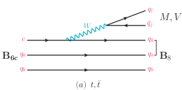
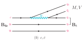
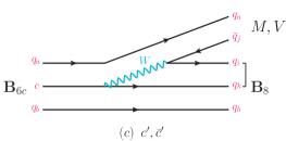
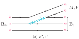
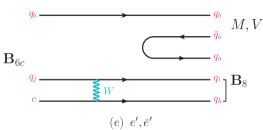
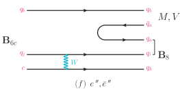
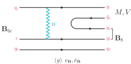
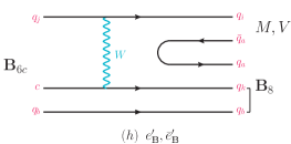
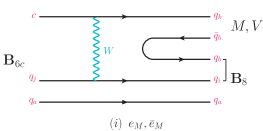
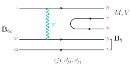
Figure 1: Topological diagrams of ${\bf B}_{6c}\to{\bf B}_{8}M(V)$ decays, where the notations “]” denote the asymmetric quark orderings of octet baryon states.

In this report, we propose the utilization of the $SU(3)_{f}$-based topological diagram approach (TDA) Kohara:1991ug ; Chau:1995gk ; Zhao:2018mov ; Wang:2020gmn ; Hsiao:2020iwc ; Pan:2020qqo ; Hsiao:2021nsc ; Hsiao:2023mud , in order to parameterize topological diagrams and establish strict $SU(3)_{f}$ relations for $\Omega_{c}^{0}$ decays. We will also employ the irreducible $SU(3)_{f}$ approach (IRA) Savage:1989qr ; Savage:1991wu ; Sharma:1996sc ; Lu:2016ogy ; Geng:2017mxn ; Geng:2017esc ; Geng:2018plk ; Geng:2018upx ; Hsiao:2019yur ; Huang:2021aqu ; Jia:2019zxi ; Zeppenfeld:1980ex ; He:2018php ; He:2018joe ; Wang:2017gxe ; Wang:2019dls ; Wang:2022kwe ; Geng:2018bow ; Huang:2021aqu ; Xing:2023dni ; Zhong:2022exp to identify dominant topological parameters. This will enable us to explore sub-processes of Figs. 1 and 2 in two-body non-leptonic $\Omega_{c}^{0}$ decays, specifically $\Omega_{c}^{0}\to{\bf B}^{(*)}M$ and $\Omega_{c}^{0}\to{\bf B}^{(*)}V$. Additionally, we will calculate branching fractions that can be experimentally measured at facilities such as Belle and LHCb.

II Formalism

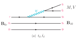
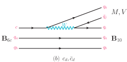
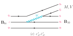
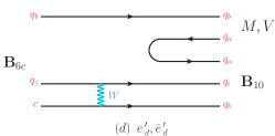
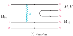
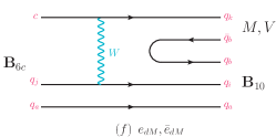
Figure 2: Topological diagrams of ${\bf B}_{6c}\to{\bf B}_{10}M(V)$ decays.

We investigate potential two-body decays of $\Omega_{c}^{0}$ that occur through the quark-level weak transitions: $c\to su\bar{d}$ and $c\to qu\bar{q}$ with $q=(d,s)$. The responsible effective Hamiltonian is defined as Buchalla:1995vs ; Buras:1998raa

$${\cal H}_{eff} = \sum_{i=+,-}\frac{G_{F}}{\sqrt{2}}c_{i}\left(V_{cs}^{*}V_{ud}O_{i}+V_{cq}^{*}V_{uq}O_{i}^{q}\right)\,.$$ (2)

Here, $G_{F}$ is the Fermi constant, $V_{ij}$ denotes the Cabibbo-Kobayashi-Maskawa (CKM) matrix element, and $c_{\pm}$ are the scale-dependent Wilson coefficients that account for perturbative QCD corrections Li:2012cfa . In Eq. (2), $O_{\pm}^{(q)}$ represent the four-quark operators, which are defined as

$$O_{\pm}={1\over 2}\left[(\bar{u}d)(\bar{s}c)\pm(\bar{s}d)(\bar{u}c)\right]\,,\;$$

$$O_{\pm}^{q}={1\over 2}\left[(\bar{u}q)(\bar{q}c)\pm(\bar{q}q)(\bar{u}c)\right]\,.$$ (3)

In the expressions above, $(\bar{q}_{1}q_{2})\equiv\bar{q}_{1}\gamma_{\mu}(1-\gamma_{5})q_{2}$.

By omitting Lorentz indices, the effective Hamiltonian in two different $SU(3)_{f}$ representations can be expressed as ${\cal H}_{eff}=(G_{F}/\sqrt{2}){\cal H}_{\rm TDA}$ and ${\cal H}_{eff}=(G_{F}/\sqrt{2}){\cal H}_{\rm IRA}$. In the context of the topological diagram approach, we consider flavor changes $c\to q_{k}q_{i}\bar{q}_{j}$ with $q_{i}=(u,d,s)$ represented as a triplet in the $SU(3)_{f}$ symmetry Pan:2020qqo ; Hsiao:2020iwc ; Hsiao:2021nsc :

$${\cal H}_{\rm{TDA}}=H_{j}^{ki}\,.$$ (4)

The non-zero entries in the equation are $H^{31}_{2}=1$ for $c\to su\bar{d}$, $H^{21}_{2}=-s_{c}$ for $c\to ud\bar{d}$, and $H^{31}_{3}=s_{c}$ for $c\to us\bar{s}$, where we have used $V_{cs}^{*}V_{ud}\simeq 1$ and $V_{cd}^{*}V_{ud}=-V_{cs}^{*}V_{us}\simeq-s_{c}$ with the Cabbibo angle $\theta_{c}$ in $s_{c}\equiv\sin\theta_{c}$.

In the irreducible $SU(3)_{f}$ approach, the operators of Eq. (II) behave as $(\bar{q}^{i}q_{k}\bar{q}^{j})c$ with respect to the $SU(3)_{f}$ symmetry, leading to $(\bar{3}\times 3\times\bar{3})c=(\bar{3}+\bar{3}^{\prime}+6+\overline{15})c$ in the irreducible form. Here, 6 and $\overline{15}$ correspond to $O_{-}\sim(\bar{u}d\bar{s}-\bar{s}d\bar{u})c$ and $O_{+}\sim(\bar{u}d\bar{s}+\bar{s}d\bar{u})c$ [$O^{q}_{-}\sim(\bar{u}q\bar{q}-\bar{q}q\bar{u})c$ and $O_{+}\sim(\bar{u}q\bar{q}+\bar{q}q\bar{u})c$], respectively. We thus obtain Savage:1989qr ; Savage:1991wu ; Geng:2017esc

$${\cal H}_{\text{IRA}}=c_{-}{\epsilon^{ijl}\over 2}H(6)_{lk}+c_{+}H(\overline{15})_{k}^{ij}\,.$$ (5)

The non-zero entries of $H(6)_{lk}$ are $H_{22}(6)=2$ and $H_{23,32}(6)=2s_{c}$, while those of $H(\overline{15})_{k}^{ij}$ are given by $H_{2}^{13}(\overline{15})=H_{2}^{31}(\overline{15})=1$ and $H_{2}^{12,21}(\overline{15})=-H_{3}^{13,31}(\overline{15})=-s_{c}$ Savage:1989qr ; Hsiao:2020iwc .

We present $\Omega_{c}^{0}$ as a sextet charmed baryon: $({\bf B}_{6c})^{3}_{3}=\Omega_{c}^{0}$, omitting other ${\bf B}_{6c}$ states that strongly decay. The octet and decuplet baryons have components:

$$({\bf B}_{8})^{i}_{j} = \left(\begin{array}[]{ccc}\frac{1}{\sqrt{6}}\Lambda^{0}+\frac{1}{\sqrt{2}}\Sigma^{0}&\Sigma^{+}&p\\ \Sigma^{-}&\frac{1}{\sqrt{6}}\Lambda^{0}-\frac{1}{\sqrt{2}}\Sigma^{0}&n\\ \Xi^{-}&\Xi^{0}&-\sqrt{\frac{2}{3}}\Lambda^{0}\end{array}\right)\,,$$ (9)

$$\sqrt{3}({\bf B}_{10})_{ijk} = \left(\begin{array}[]{ccc}\left(\begin{array}[]{ccc}\sqrt{3}\Delta^{++}&\Delta^{+}&\Sigma^{*+}\\ \Delta^{+}&\Delta^{0}&\frac{\Sigma^{*0}}{\sqrt{2}}\\ \Sigma^{*+}&\frac{\Sigma^{*0}}{\sqrt{2}}&\Xi^{*0}\end{array}\right),\left(\begin{array}[]{ccc}\Delta^{+}&\Delta^{0}&\frac{\Sigma^{*0}}{\sqrt{2}}\\ \Delta^{0}&\sqrt{3}\Delta^{-}&\Sigma^{*-}\\ \frac{\Sigma^{*0}}{\sqrt{2}}&\Sigma^{*-}&\Xi^{*-}\end{array}\right),\left(\begin{array}[]{ccc}\Sigma^{*+}&\frac{\Sigma^{*0}}{\sqrt{2}}&\Xi^{*0}\\ \frac{\Sigma^{*0}}{\sqrt{2}}&\Sigma^{*-}&\Xi^{*-}\\ \Xi^{*0}&\Xi^{*-}&\sqrt{3}\Omega^{-}\end{array}\right)\end{array}\right).$$ (20)

We also present the octet baryon as $({\bf B}_{8})_{ijk}=\epsilon_{ijl}({\bf B}_{8})^{l}_{k}$. As for another final state, the usual octet pseudoscalar (vector) meson $M$($V$) has components:

$$M^{i}_{j} = (\pi^{\pm,0},\;K^{\pm},\;K^{0},\;\bar{K}^{0},\;\eta)\,,$$

$$V^{i}_{j} = (\rho^{\pm,0},\;K^{*\pm},\;K^{*0},\;\bar{K}^{*0},\;\omega,\;\phi)\,.$$ (21)

We connect ${\bf B}_{6c}$ to ${\cal H}_{\rm TDA}$, ${\bf B}_{8}$, and $M$ to derive the TDA amplitudes as follows:

$${\cal M}_{\rm TDA}(\Omega_{c}^{0}\to{\bf B}_{8}M)$$

$$=t({\bf B}_{6c})^{ab}H^{ki}_{j}({\bf B}_{8})_{kab}(M)_{j}^{i}+c({\bf B}_{6c})^{ab}H^{ki}_{j}({\bf B}_{8})_{iab}(M)_{j}^{k}\,$$

$$+c^{\prime}({\bf B}_{6c})^{ab}H^{ki}_{j}({\bf B}_{8})_{ikb}(M)_{j}^{a}+c^{\prime\prime}({\bf B}_{6c})^{ab}H^{ki}_{j}({\bf B}_{8})_{ibk}(M)_{j}^{a}\,$$

$$+e^{\prime}({\bf B}_{6c})^{jb}H^{ki}_{j}({\bf B}_{8})_{ika}(M)_{a}^{b}+e^{\prime\prime}({\bf B}_{6c})^{jb}H^{ki}_{j}({\bf B}_{8})_{iak}(M)_{a}^{b}\,$$

$$+e_{\bf B}({\bf B}_{6c})^{jb}H^{ki}_{j}({\bf B}_{8})_{kab}(M)_{a}^{i}+e^{\prime}_{\bf B}({\bf B}_{6c})^{jb}H^{ki}_{j}({\bf B}_{8})_{kba}(M)_{a}^{i}\,$$

$$+e_{M}({\bf B}_{6c})^{jb}H^{ki}_{j}({\bf B}_{8})_{iba}(M)_{a}^{k}+e_{M}^{\prime}({\bf B}_{6c})^{jb}H^{ki}_{j}({\bf B}_{8})_{iab}(M)_{a}^{k}\,.$$ (22)

In this equation, the parameters $t$, $c$, $c^{\prime(\prime\prime)}$, $e^{\prime(\prime\prime)}$, $e_{\bf B}^{(\prime)}$, and $e_{M}^{(\prime)}$ correspond to the decay topological diagrams in Figs. 1a, 1b, 1c(d), 1e(f), 1g(h), and 1i(j), respectively. Figs. 1$a$ and 1$(b,c,d)$ represent the external and internal $W$-emission diagrams, respectively, while Figs. 1$(e,f,g,h,i,j)$ depict the $W$-exchange diagrams. Specifically, $e_{\bf B}$ and $e_{M}$ correspond to the topological diagrams where the charm quark transforms into ${\bf B}$ and $M$, respectively. In contrast, $e^{\prime}$ represents a topological diagram where the $W$-exchange exclusively occurs within ${\bf B}$ without involving $M$. Furthermore, $c^{\prime\prime}$, $e^{\prime\prime}$ and $e^{\prime}_{{\bf B}(M)}$ parameterize the same topological diagrams as $c^{\prime}$, $e^{\prime}$ and $e_{{\bf B}(M)}$, respectively, but with a different anti-symmetric quark pair in ${\bf B}$.

The decuplet baryon consists of quark contents that are totally symmetric, resulting in six topological diagrams for $\Omega_{c}^{0}\to{\bf B}_{10}M$ as drawn in Fig. 2. The amplitudes are then derived as

$${\cal M}_{\rm TDA}(\Omega_{c}^{0}\to{\bf B}_{10}M)$$

$$=t_{d}({\bf B}_{6c})^{ab}H^{ki}_{j}({\bf B}_{10})_{kab}(M)_{j}^{i}+c_{d}({\bf B}_{6c})^{ab}H^{ki}_{j}({\bf B}_{10})_{iab}(M)_{j}^{k}\,$$

$$+c_{d}^{\prime}({\bf B}_{6c})^{ab}H^{ki}_{j}({\bf B}_{10})_{ikb}(M)_{j}^{a}+e_{d}^{\prime}({\bf B}_{6c})^{jb}H^{ki}_{j}({\bf B}_{10})_{ika}(M)_{a}^{b}\,$$

$$+e_{d{\bf B}}({\bf B}_{6c})^{jb}H^{ki}_{j}({\bf B}_{10})_{kab}(M)_{a}^{i}+e_{dM}({\bf B}_{6c})^{jb}H^{ki}_{j}({\bf B}_{10})_{iba}(M)_{a}^{k}\,.$$ (23)

Here, $(t_{d},c_{d},c^{\prime}_{d})$ and $(e^{\prime}_{d},e_{d{\bf B}},e_{dM})$ paramterize the $W$-emission and $W$-exchange topological diagrams of Figs. 2$(a,b,c)$ and Figs. 2$(d,e,f)$, respectively.

Table 1: ${\cal M}_{\rm{TDA,IRA}}(\Omega_{c}^{0}\to{\bf B}M(V))$ from the expansions in Eqs. (II) and (24), respectively.

Decay mode	${\cal M}_{\text{TDA}}$	${\cal M}_{\text{IRA}}$
$\Omega_{c}^{0}\to\Xi^{0}\bar{K}^{0}$	$-(c+c^{\prime})$	$2a_{13}-a_{16}-a_{17}$
$\Omega_{c}^{0}\to\Lambda^{0}\bar{K}^{0}$	$\frac{1}{\sqrt{6}}(2c^{\prime}+c^{\prime\prime}-e_{M}-2e_{M}^{\prime}-e^{\prime}-2e^{\prime\prime})s_{c}$	$\frac{-1}{\sqrt{6}}(4a_{13}+4a_{14}-2a_{15}-3a_{16}-2a_{17}+a_{18}-3a_{19}-2a_{20})s_{c}$
$\Omega_{c}^{0}\to\Sigma^{0}\bar{K}^{0}$	$\frac{1}{\sqrt{2}}(e_{M}+e^{\prime}-c^{\prime\prime})s_{c}$	$\frac{-1}{\sqrt{2}}(2a_{15}+a_{16}-a_{18}-a_{19})s_{c}$
$\Omega_{c}^{0}\to\Sigma^{+}K^{-}$	$-(e_{{M}}+e^{\prime})s_{c}$	$(2a_{15}-a_{16}+a_{18}+a_{19})s_{c}$
$\Omega_{c}^{0}\to\Xi^{-}\pi^{+}$	$-(t+e_{{\bf B}})s_{c}$	$(2a_{14}+a_{20})s_{c}$
$\Omega_{c}^{0}\to\Xi^{0}\pi^{0}$	$\frac{-1}{\sqrt{2}}(c-e_{{\bf B}})s_{c}$	$\frac{-1}{\sqrt{2}}(2a_{14}+2a_{17}+a_{20})s_{c}$
$\Omega_{c}^{0}\to\Xi^{0}\eta$	$\frac{1}{\sqrt{6}}(3c+2c^{\prime}+2c^{\prime\prime}+e_{\bf{B}}+2e_{M}+2e_{M}^{\prime}+2e^{\prime}+2e^{\prime\prime})s_{c}$	$\frac{-1}{\sqrt{6}}(4a_{13}-2a_{14}+4a_{15}-2a_{18}+2a_{19}+3a_{20})s_{c}$
$\Omega_{c}^{0}\to\Xi^{0}\bar{K}^{*0}$	$-(\bar{c}+\bar{c}^{\prime})$	$2\bar{a}_{13}-\bar{a}_{16}-\bar{a}_{17}$
$\Omega_{c}^{0}\to\Lambda^{0}\bar{K}^{*0}$	$\frac{1}{\sqrt{6}}(2\bar{c}^{\prime}+\bar{c}^{\prime\prime}-\bar{e}_{M}-2\bar{e}_{M}^{\prime}-\bar{e}^{\prime}-2\bar{e}^{\prime\prime})s_{c}$	$\frac{-1}{\sqrt{6}}(4\bar{a}_{13}+4\bar{a}_{14}-2\bar{a}_{15}-3\bar{a}_{16}-2\bar{a}_{17}+\bar{a}_{18}-3\bar{a}_{19}-2\bar{a}_{20})s_{c}$
$\Omega_{c}^{0}\to\Sigma^{0}\bar{K}^{*0}$	$\frac{1}{\sqrt{2}}(\bar{e}_{M}+\bar{e}^{\prime}-\bar{c}^{\prime\prime})s_{c}$	$\frac{-1}{\sqrt{2}}(2\bar{a}_{15}+\bar{a}_{16}-\bar{a}_{18}-\bar{a}_{19})s_{c}$
$\Omega_{c}^{0}\to\Sigma^{+}K^{*-}$	$-(\bar{e}_{{M}}+\bar{e}^{\prime})s_{c}$	$(2\bar{a}_{15}-\bar{a}_{16}+\bar{a}_{18}+\bar{a}_{19})s_{c}$
$\Omega_{c}^{0}\to\Xi^{-}\rho^{+}$	$-(\bar{t}+\bar{e}_{{\bf B}})s_{c}$	$(2\bar{a}_{14}+\bar{a}_{20})s_{c}$
$\Omega_{c}^{0}\to\Xi^{0}\rho^{0}$	$\frac{-1}{\sqrt{2}}(\bar{c}-\bar{e}_{{\bf B}})s_{c}$	$\frac{-1}{\sqrt{2}}(2\bar{a}_{14}+2\bar{a}_{17}+\bar{a}_{20})s_{c}$
$\Omega_{c}^{0}\to\Xi^{0}\omega$	$\frac{1}{\sqrt{2}}(\bar{c}+\bar{e}_{\bf{B}})s_{c}$	$\frac{1}{\sqrt{2}}(2\bar{a}_{14}-\bar{a}_{20})s_{c}$
$\Omega_{c}^{0}\to\Xi^{0}\phi$	$-(\bar{c}+\bar{c}^{\prime}+\bar{c}^{\prime\prime}+\bar{e}_{M}+\bar{e}_{M}^{\prime}+\bar{e}^{\prime}+\bar{e}^{\prime\prime})s_{c}$	$(2\bar{a}_{13}+2\bar{a}_{15}-\bar{a}_{18}+\bar{a}_{19}+\bar{a}_{20})s_{c}$

Similar to TDA, we connect ${\bf B}_{6c}$ to ${\cal H}_{\rm IRA}$, ${\bf B}_{8(10)}$, and $M$ to establish the IRA amplitudes for $\Omega_{c}^{0}\to{\bf B}_{8(10)}M$. For $\Omega_{c}^{0}\to{\bf B}_{8}M$, the amplitudes are given by

$${\cal M}_{\rm IRA}(\Omega_{c}^{0}\to{\bf B}_{8}M)={\cal M}_{6}+{\cal M}_{\overline{15}}\,,$$ (24)

where Savage:1989qr ; Geng:2017mxn

$${\cal M}_{6}=a_{12}H_{ij}(6)({\bf B}_{6c})^{ij}({\bf B}_{8})_{k}^{l}(M)_{l}^{k}+a_{13}H_{ij}(6)({\bf B}_{6c})^{kl}({\bf B}_{8})_{k}^{i}(M)_{l}^{j}$$

$$+a_{14}H_{ij}(6)({\bf B}_{6c})^{jk}({\bf B}_{8})_{k}^{l}(M)_{l}^{i}+a_{15}H_{ij}(6)({\bf B}_{6c})^{jk}({\bf B}_{8})_{l}^{i}(M)_{k}^{l}\,,$$

$${\cal M}_{\overline{15}}=a_{16}({\bf B}_{8})_{j}^{i}(M)_{l}^{k}H(\overline{15})^{jm}_{i}({\bf B}_{6c})^{ln}\epsilon_{kmn}+a_{17}({\bf B}_{8})_{j}^{i}(M)_{l}^{k}H(\overline{15})^{lm}_{i}({\bf B}_{6c})^{jn}\epsilon_{kmn}$$

$$+a_{18}({\bf B}_{8})_{n}^{m}(M)_{j}^{n}H(\overline{15})^{ij}_{k}({\bf B}_{6c})^{kl}\epsilon_{ilm}+a_{19}({\bf B}_{8})_{l}^{j}(M)_{n}^{k}H(\overline{15})^{il}_{m}({\bf B}_{6c})^{mn}\epsilon_{ijk}$$

$$+a_{20}({\bf B})_{n}^{j}(M)_{l}^{k}H(\overline{15})^{il}_{m}({\bf B}_{6c})^{mn}\epsilon_{ijk}\,.$$ (25)

The parameters $a_{i}$ (with $i$ ranging from 12 to 20) represent the $SU(3)_{f}$ invariant amplitudes. For $\Omega_{c}^{0}\to{\bf B}_{10}M$, we express the amplitudes to be Savage:1989qr ; Geng:2017mxn

$${\cal M}_{\rm IRA}(\Omega_{c}^{0}\to{\bf B}_{10}M)={\cal M}^{\prime}_{6}+{\cal M}^{\prime}_{\overline{15}}\,,$$ (26)

where ${\cal M}^{\prime}_{6}$ and ${\cal M}^{\prime}_{\overline{15}}$ are defined similarly to ${\cal M}_{6}$ and ${\cal M}_{\overline{15}}$, respectively, given by

$${\cal M}^{\prime}_{6}=a_{21}({\bf B}_{10})_{lkm}(M)_{n}^{i}H_{ij}(6)({\bf B}_{6c})^{lk}\epsilon^{jmn}+a_{22}({\bf B}_{10})_{klm}(M)_{n}^{l}H_{ij}(6)({\bf B}_{6c})^{jk}\epsilon^{imn}\,,$$

$${\cal M}^{\prime}_{\overline{15}}=a_{23}({\bf B}_{10})_{ijk}(M)_{l}^{m}H(\overline{15})^{lk}_{m}({\bf B}_{6c})^{ij}+a_{24}({\bf B}_{10})_{ijk}(M)_{m}^{k}H(\overline{15})^{ij}_{l}({\bf B}_{6c})^{lm}$$

$$+a_{25}({\bf B}_{10})_{ijk}(M)_{m}^{l}H(\overline{15})^{ij}_{l}({\bf B}_{6c})^{km}+a_{26}({\bf B}_{10})_{ijk}(M)_{l}^{j}H(\overline{15})^{lk}_{m}({\bf B}_{6c})^{im}\,.$$ (27)

The parameters $a_{i}$ (with $i$ ranging from 21 to 26) are another set of the $SU(3)_{f}$ parameters.

Table 2: ${\cal M}_{\rm{TDA,IRA}}(\Omega_{c}^{0}\to{\bf B}^{*}M(V))$ from the expansions in Eqs. (II) and (26), respectively.

Decay mode	${\cal M}_{\text{TDA}}$	${\cal M}_{\text{IRA}}$
$\Omega_{c}^{0}\to\Xi^{*0}\bar{K}^{0}$	$\frac{1}{\sqrt{3}}(c_{d}+c^{\prime}_{d})$	$\frac{-1}{\sqrt{3}}(2a_{21}-a_{23}-2a_{25})$
$\Omega_{c}^{0}\to\Omega^{-}\pi^{+}$	$t_{d}$	$2a_{21}+a_{23}$
$\Omega_{c}^{0}\to\Omega^{-}K^{+}$	$(t_{d}+e_{d{\bf B}})s_{c}$	$(2a_{21}+2a_{22}+a_{23}+a_{26})s_{c}$
$\Omega_{c}^{0}\to\Sigma^{*+}K^{-}$	$\frac{1}{\sqrt{3}}(e_{dM}+e^{\prime}_{d})s_{c}$	$\frac{-1}{\sqrt{3}}(2a_{22}-2a_{24}-a_{26})s_{c}$
$\Omega_{c}^{0}\to\Sigma^{*0}\bar{K}^{0}$	$\frac{-1}{\sqrt{6}}(c^{\prime}_{d}-e_{dM}-e^{\prime}_{d})s_{c}$	$\frac{-1}{\sqrt{6}}(2a_{22}-2a_{24}+2a_{25}-a_{26})s_{c}$
$\Omega_{c}^{0}\to\Xi^{*-}\pi^{+}$	$\frac{-1}{\sqrt{3}}(t_{d}-e_{d{\bf B}})s_{c}$	$\frac{-1}{\sqrt{3}}(2a_{21}-2a_{22}+a_{23}-a_{26})s_{c}$
$\Omega_{c}^{0}\to\Xi^{*0}\pi^{0}$	$\frac{1}{\sqrt{6}}(c_{d}+e_{d{\bf B}})s_{c}$	$\frac{-1}{\sqrt{6}}(2a_{21}-2a_{22}-a_{23}-a_{26})s_{c}$
$\Omega_{c}^{0}\to\Xi^{*0}\eta$	$\frac{-1}{\sqrt{1}8}(3c_{d}+2c^{\prime}_{d}-e_{d{\bf B}}+2e_{dM}+2e^{\prime}_{d})s_{c}$	$\frac{-1}{\sqrt{1}8}(6a_{21}+6a_{22}-3a_{23}-24a_{24}-4a_{25}-a_{26})s_{c}$
$\Omega_{c}^{0}\to\Xi^{*0}\bar{K}^{*0}$	$\frac{1}{\sqrt{3}}(\bar{c}_{d}+\bar{c}^{\prime}_{d})$	$\frac{-1}{\sqrt{3}}(2\bar{a}_{21}-\bar{a}_{23}-2\bar{a}_{25})$
$\Omega_{c}^{0}\to\Omega^{-}\rho^{+}$	$\bar{t}_{d}$	$2\bar{a}_{21}+\bar{a}_{23}$
$\Omega_{c}^{0}\to\Omega^{-}K^{*+}$	$(\bar{t}_{d}+\bar{e}_{d{\bf B}})s_{c}$	$(2\bar{a}_{21}+2\bar{a}_{22}+\bar{a}_{23}+\bar{a}_{26})s_{c}$
$\Omega_{c}^{0}\to\Sigma^{*+}K^{*-}$	$\frac{1}{\sqrt{3}}(\bar{e}_{dM}+\bar{e}^{\prime}_{d})s_{c}$	$\frac{-1}{\sqrt{3}}(2\bar{a}_{22}-2\bar{a}_{24}-\bar{a}_{26})s_{c}$
$\Omega_{c}^{0}\to\Sigma^{*0}\bar{K}^{*0}$	$\frac{-1}{\sqrt{6}}(\bar{c}^{\prime}_{d}-\bar{e}_{dM}-\bar{e}^{\prime}_{d})s_{c}$	$\frac{-1}{\sqrt{6}}(2\bar{a}_{22}-2\bar{a}_{24}+2\bar{a}_{25}-\bar{a}_{26})s_{c}$
$\Omega_{c}^{0}\to\Xi^{*-}\rho^{+}$	$\frac{-1}{\sqrt{3}}(\bar{t}_{d}-\bar{e}_{d{\bf B}})s_{c}$	$\frac{-1}{\sqrt{3}}(2\bar{a}_{21}-2\bar{a}_{22}+\bar{a}_{23}-\bar{a}_{26})s_{c}$
$\Omega_{c}^{0}\to\Xi^{*0}\rho^{0}$	$\frac{1}{\sqrt{6}}(\bar{c}_{d}+\bar{e}_{d{\bf B}})s_{c}$	$\frac{-1}{\sqrt{6}}(2\bar{a}_{21}-2\bar{a}_{22}-\bar{a}_{23}-\bar{a}_{26})s_{c}$
$\Omega_{c}^{0}\to\Xi^{*0}\omega$	$\frac{-1}{\sqrt{6}}(\bar{c}_{d}-\bar{e}_{d{\bf B}})s_{c}$	$\frac{1}{\sqrt{6}}(2\bar{a}_{21}+2\bar{a}_{22}-\bar{a}_{23}+\bar{a}_{26})s_{c}$
$\Omega_{c}^{0}\to\Xi^{*0}\phi$	$\frac{1}{\sqrt{3}}(\bar{c}_{d}+\bar{c}^{\prime}_{d}+\bar{e}_{dM}+\bar{e}^{\prime}_{d})s_{c}$	$\frac{-1}{\sqrt{3}}(2\bar{a}_{21}+2\bar{a}_{22}-\bar{a}_{23}-2\bar{a}_{24}-2\bar{a}_{25}-\bar{a}_{26})s_{c}$

Using ${\cal M}_{\rm TDA}(\Omega_{c}^{0}\to{\bf B}^{(*)}M)={\cal M}_{\rm IRA}(\Omega_{c}^{0}\to{\bf B}^{(*)}M)$, with expansions provided in Tables 1 and 2, we establish the following relations:

$$(t,c,c^{\prime},c^{\prime\prime})=(-2a_{14}+a_{17},2a_{14}+a_{17},-2a_{13}-2a_{14},0)\,,$$ (28)

$$(e^{\prime},e^{\prime\prime})=(-2a_{12}-2a_{15}+a_{19},-2a_{19})\,,$$

$$(e_{\bf B},e^{\prime}_{M})=(-a_{17}-a_{20},-a_{17}-a_{20})\,,$$

$$(e_{M},e^{\prime}_{\bf B})=(2a_{12}+a_{18},-2a_{12}+a_{18})\,,$$

for $\Omega_{c}^{0}\to{\bf B}M$. Note that the parameter $e^{\prime}_{\bf B}$ only appears in the doubly Cabibbo-suppressed decay channels, such as ${\cal M}(\Omega_{c}^{0}\to\Sigma^{-}\pi^{+})$, which are not within the scope of the current study. However, $e^{\prime}_{\bf B}$ is included in Eq. (28) to complete the relations. Additionally, we obtain the following relations for $\Omega_{c}^{0}\to{\bf B}^{*}M$:

$$(t_{d},c_{d},c^{\prime}_{d},e^{\prime}_{d})=(2a_{21}+a_{23},-2a_{21}+a_{23},2a_{25},2a_{24})\,,$$

$$(e_{d\bf B},e_{dM})=(2a_{22}+a_{26},-2a_{22}+a_{26})\,.$$ (29)

These results demonstrate the equivalence of the two $SU(3)_{f}$ methods for the two-body non-leptonic $\Omega_{c}^{0}\to{\bf B}^{(*)}M$ weak decays He:2018php ; He:2018joe ; Hsiao:2020iwc ; Hsiao:2021nsc .

Both TDA and IRA have their own advantages. For example, TDA is associated with intuitive topological diagrams that help us visualize the decay processes of $\Omega_{c}^{0}\to{\bf B}M,{\bf B}^{*}M$. On the other hand, IRA identifies dominant parameters. This is due to the fact that perturbative QCD corrections to the quark currents lead to a ratio of $c_{-}/c_{+}\sim 2.5$ Savage:1989qr ; Lu:2016ogy ; Li:2012cfa in ${\cal H}_{\text{IRA}}\propto c_{-}H(6)_{lk}+c_{+}H(\overline{15})$ of Eq. (5). As a result, $(a_{12},a_{13},a_{14},a_{15})$ for $\Omega_{c}^{0}\to{\bf B}M$ and $(a_{21},a_{22})$ for $\Omega_{c}^{0}\to{\bf B}^{*}M$ absorb $c_{-}$ and become the dominant ones, while the parameters associated with $c_{+}H(\overline{15})$ are commonly negligible Lu:2016ogy ; Geng:2017mxn ; Geng:2018bow ; Geng:2017esc ; Geng:2018plk ; Geng:2018upx ; Hsiao:2019yur .

Thus, the relations of Eqs. (28) and (II) are reduced to

$$t=-c=-2a_{14}\,,c^{\prime}=-2a_{13}-2a_{14}\,,e^{\prime}=-e_{M}=e^{\prime}_{\bf B}=-2a_{12}\,,$$

$$t_{d}=-c_{d}=2a_{21}\,,e_{d\bf B}=-e_{dM}=2a_{22}\,.$$ (30)

Meanwhile, $(c^{\prime\prime},e^{\prime\prime},e_{\bf B},e^{\prime}_{M})$ and $(c^{\prime}_{d},e^{\prime}_{d})$ are neglected in this unification.

It is worth noting that, in one way or another, the terms $c^{\prime\prime}$ and $e^{\prime\prime}$ should be neglected. As pointed out by Ref. Kohara:1991ug , this neglect is grounded in the K$\ddot{\text{o}}$rner-Pati-Woo theorem Miura:1967lka ; Korner:1970xq ; Pati:1970fg , which states that in weak currents such as $(\bar{q}_{i}q_{j})(\bar{q}_{k}c)$, the quarks $q_{i}$ and $q_{k}$, when connected by an exchange of a $W$-boson, should exhibit color anti-symmetry. This leads to their flavor anti-symmetry as the constituents of the octet baryon. As illustrated in Fig. 1, the use of $c^{\prime}$ and $e^{\prime}$, rather than $c^{\prime\prime}$ and $e^{\prime\prime}$, adheres to this theorem.

By adding the bar notation to the parameters and replacing $(M)^{i}_{j}$ with $(V)^{i}_{j}$ in Eqs. (II, II) and Eqs. (24, 26), we get ${\cal M}_{\rm TDA,IRA}(\Omega_{c}^{0}\to{\bf B}^{(*)}V)$ as given in Tables 1 and 2, resulting in the unified relations the same as in Eqs. (28, II) and (II) except for the added bar notation. As a consequence, we simplify the TDA amplitudes as ${\cal M}_{\rm STDA}(\Omega_{c}^{0}\to{\bf B}^{(*)}M,{\bf B}^{(*)}V)$ using the relations in Eq. (II), listed in Table 3. We need an equation to turn the amplitude into the branching fraction, given by pdg

$${\cal B}(\Omega_{c}^{0}\to{\bf B}^{(*)}M,{\bf B}^{(*)}V)=\frac{G_{F}^{2}|\vec{p}_{\rm cm}|\tau_{\Omega_{c}}}{16\pi m_{\Omega_{c}}^{2}}|{\cal M}_{\rm STDA}(\Omega_{c}^{0}\to{\bf B}^{(*)}M,{\bf B}^{(*)}V)|^{2}\,,$$ (31)

with $|\vec{p}_{\rm cm}|=[(m_{\Omega_{c}}^{2}-m_{+}^{2})(m_{\Omega_{c}}^{2}-m_{-}^{2})]^{1/2}/(2m_{\Omega_{c}})$, where $m_{\pm}=m_{{\bf B}^{(*)}}\pm m_{M(V)}$, $\tau_{\Omega_{c}}$ stands for the lifetime of $\Omega_{c}^{0}$, and $\vec{p}_{cm}$ is the three-momentum of the final state in the $\Omega_{c}^{0}$ rest frame.

III Numerical Analysis

To perform a numerical analysis, we use the Wolfenstein parameter $\lambda=s_{c}=0.225$ to present the CKM matrix elements as pdg

$$(V_{cs},V_{ud},V_{us},V_{cd})=(1-\lambda^{2}/2,1-\lambda^{2}/2,\lambda,-\lambda)\,.$$ (32)

Using one theoretical branching fraction as an input for the experimental rates in Eq. (I), we can extract additional information. As for the candidates, the branching fractions of $\Omega_{c}^{0}\to\Omega^{-}e^{+}\nu_{e}$, $\Omega^{-}\pi^{+}$, and $\Omega^{-}\rho^{+}$ have been calculated with the $\Omega_{c}^{0}\to\Omega^{-}$ transition form factors studied in Pervin:2006ie ; Hsiao:2020gtc ; Xu:1992sw ; Cheng:1996cs ; Gutsche:2018utw . Since the semileptonic decay involves a lepton pair free from QCD corrections Hsiao:2023qtk ; Ke:2023qzc , ${\cal B}_{e}\equiv{\cal B}(\Omega_{c}^{0}\to\Omega^{-}e^{+}\nu_{e})$ can be considered more reliable than ${\cal B}(\Omega_{c}^{0}\to\Omega^{-}\pi^{+},\Omega^{-}\rho^{+})$. Therefore, we follow Ref. Hsiao:2020gtc to calculate ${\cal B}_{e}=(5.4\pm 0.2)\times 10^{-3}$. By relating ${\cal B}_{e}$ to ${\cal R}_{e}$ in Eq. (I), we extract ${\cal B}_{\pi}\equiv{\cal B}(\Omega_{c}^{0}\to\Omega^{-}\pi^{+})=(29.6\pm 2.5)\times 10^{-4}$, instead of calculating it. We then use ${\cal B}_{\pi}$ to extract other absolute branching ratios, as given in Table 3.

The study of the branching fractions relies on the determination of the topological parameters of ${\cal M}_{\rm STDA}$ in Table 3, that is, $(t,c^{\prime})$ for $\Omega_{c}^{0}\to{\bf B}M$, $(\bar{t},\bar{c}^{\prime})$ for $\Omega_{c}^{0}\to{\bf B}V$, $(t_{d},e_{dM})$ for $\Omega_{c}^{0}\to{\bf B}^{*}M$, and $(\bar{t}_{d},\bar{e}_{dM})$ for $\Omega_{c}^{0}\to{\bf B}^{*}V$, where $c_{(d)}=-t_{(d)}$ and $\bar{c}_{(d)}=-\bar{t}_{(d)}$. We can use the absolute branching fractions in Table 3 to extract the topological parameters. By utilizing ${\cal B}(\Omega_{c}^{0}\to\Xi^{0}\bar{K}^{0},\Xi^{-}\pi^{+})=(48.5\pm 9.5,4.8\pm 0.5)\times 10^{-4}$ and ${\cal B}(\Omega_{c}^{0}\to\Omega^{-}\pi^{+},\Omega^{-}K^{+})=(29.6\pm 2.5,1.8\pm 0.3)\times 10^{-4}$ in Table 3 as the data inputs, associated with ${\cal M}_{\rm STDA}(\Omega_{c}^{0}\to\Xi^{0}\bar{K}^{0},\Xi^{-}\pi^{+})$ and ${\cal M}_{\rm STDA}(\Omega_{c}^{0}\to\Omega^{-}\pi^{+},\Omega^{-}K^{+})$, respectively, we can determine the values of $(t,c^{\prime})$ and $(t_{d},e_{dM})$.

For $\Omega_{c}^{0}\to{\bf B}V$, the single data point in Table 3 is not sufficient to determine $\bar{t}$ and $\bar{c}^{\prime}$ simultaneously. The fact that the terms represented by $t$ and $\bar{t}$ correspond to the factorizable amplitudes Hsiao:2020gtc ; Hsiao:2021mlp :

$${\cal M}_{\rm fac}(\Omega_{c}^{0}\to{\bf B}M,{\bf B}V)=\frac{G_{F}}{\sqrt{2}}V_{cq}^{*}V_{q_{1}q_{2}}a_{1}\langle M,V|(\bar{q}_{1}q_{2})|0\rangle\langle{\bf B}|(\bar{q}c)|\Omega_{c}^{0}\rangle\,,$$ (33)

can be helpful to perform a practical determination. Hence, we calculate the branching fraction of $\Omega_{c}^{0}\to\Xi^{-}\pi^{+}$ based on Eq. (33) and the $\Omega_{c}^{0}\to\Xi^{-}$ transition form factors in Hu:2020nkg . By connecting our calculation to the data input to be ${\cal B}_{\rm fac}(\Omega_{c}^{0}\to\Xi^{-}\pi^{+})=(4.8\pm 0.5)\times 10^{-4}$, we extract $a_{1}=0.94\pm 0.05$. We then use $a_{1}$ as an input to get the numerical result: ${\cal B}(\Omega_{c}^{0}\to\Xi^{-}\rho^{+})=(16.6\pm 1.2)\times 10^{-4}$. In addition to ${\cal B}(\Omega_{c}^{0}\to\Xi^{0}\bar{K}^{*0})=(30.2\pm 7.5)\times 10^{-4}$ in Table 3, we can have two inputs to get $\bar{t}$ and $\bar{c}^{\prime}$ simultaneously.

With ${\cal B}(\Omega_{c}^{0}\to\Xi^{*0}\bar{K}^{*0},\Omega^{-}\rho^{+})=(15.1\pm 5.2,53.3\pm 10.8)\times 10^{-4}$, we can fit $\bar{t}_{d}$, whereas the branching fraction for $\bar{e}_{dM}$ has not been measured yet. Therefore, we assume that $\bar{e}_{dM}=(e_{dM}/t_{d})\bar{t}_{d}$. Here, we summarize the determined parameters and provide the numerical results as follows:

$$(t,\bar{t})=(0.25\pm 0.01,0.52\pm 0.02)~{}{\rm GeV}^{3}\,,$$

$$(t_{d},\bar{t}_{d})=(0.16\pm 0.01,0.26\pm 0.02)~{}{\rm GeV}^{3}\,.$$ (34)

There exist two solutions of the non-factorizable parameters, depending on how they interfere with the $t$-like terms $(t_{(d)},\bar{t}_{(d)})$, as given below:

$${\rm\bullet~{}Solution~{}1}$$

$$(c^{\prime},\bar{c}^{\prime})=(0.44\pm 0.01,0.69\pm 0.01)~{}{\rm GeV}^{3}\,,$$

$$(e_{dM},\bar{e}_{dM})=(0.35\pm 0.01,0.57\pm 0.06)~{}{\rm GeV}^{3}\,,$$

$${\rm\bullet~{}Solution~{}2}$$

$$(c^{\prime},\bar{c}^{\prime})=(0.06\pm 0.01,0.35\pm 0.01)~{}{\rm GeV}^{3}\,,$$

$$(e_{dM},\bar{e}_{dM})=(-0.02\pm 0.01,-0.03\pm 0.02)~{}{\rm GeV}^{3}\,,$$ (35)

where the errors include the uncertainties from the data inputs. Subsequently, we define two scenarios, denoted as $(S1,S2)$ for predicting the branching fractions. These scenarios consider the $t$-like terms from Eq. (III) and two sets of the non-factorizable parameters based on Solution 1 and Solution 2 as outlined in Eq. (III). The results for these two scenarios can be found in Table 3.

Table 3: ${\cal M}_{\text{STDA}}(\Omega_{c}^{0}\to{\bf B}^{(*)}M,{\bf B}^{(*)}V)$ with STDA denoting the simplified TDA, the data inputs, together with our work and the data inputs for the branching fractions.

Decay mode	${\cal M}_{\rm{STDA}}$	${\cal B}\times 10^{4}$ (our work: S1, S2)	${\cal B}\times 10^{4}$ (data input)
$\Omega_{c}^{0}\to\Xi^{0}\bar{K}^{0}$	$-(c+c^{\prime})$	$(47.0\pm 7.2,47.0\pm 7.2)$	$48.5\pm 9.5$
$\Omega_{c}^{0}\to\Lambda^{0}\bar{K}^{0}$	$\frac{2}{\sqrt{6}}c^{\prime}s_{c}$	$(9.0\pm 0.4,0.2\pm 0.1)$
$\Omega_{c}^{0}\to\Sigma^{+}K^{-}$	$0$	$<1$
$\Omega_{c}^{0}\to\Sigma^{0}\bar{K}^{0}$	$0$	$<1$
$\Omega_{c}^{0}\to\Xi^{-}\pi^{+}$	$-ts_{c}$	$(4.7\pm 0.4,4.7\pm 0.4)$	$4.8\pm 0.5$
$\Omega_{c}^{0}\to\Xi^{0}\pi^{0}$	$\frac{-1}{\sqrt{2}}cs_{c}$	$(2.3\pm 0.2,2.3\pm 0.2)$
$\Omega_{c}^{0}\to\Xi^{0}\eta$	$\frac{1}{\sqrt{6}}(3c+2c^{\prime})s_{c}$	$(0.2\pm 0.1,4.5\pm 0.5)$
$\Omega_{c}^{0}\to\Xi^{0}\bar{K}^{*0}$	$-(\bar{c}+\bar{c}^{\prime})$	$(30.2\pm 8.4,30.2\pm 8.4)$	$30.2\pm 7.5$
$\Omega_{c}^{0}\to\Lambda^{0}\bar{K}^{*0}$	$\frac{2}{\sqrt{6}}\bar{c}^{\prime}s_{c}$	$(17.7\pm 0.5,4.6\pm 0.3)$
$\Omega_{c}^{0}\to\Sigma^{+}K^{*-}$	$0$	$<1$
$\Omega_{c}^{0}\to\Sigma^{0}\bar{K}^{*0}$	$0$	$<1$
$\Omega_{c}^{0}\to\Xi^{-}\rho^{+}$	$-\bar{t}s_{c}$	$(16.4\pm 1.3,16.4\pm 1.3)$
$\Omega_{c}^{0}\to\Xi^{0}\rho^{0}$	$\frac{-1}{\sqrt{2}}\bar{c}s_{c}$	$(8.2\pm 0.6,8.2\pm 0.6)$
$\Omega_{c}^{0}\to\Xi^{0}\omega$	$\frac{1}{\sqrt{2}}\bar{c}s_{c}$	$(8.2\pm 0.6,8.2\pm 0.6)$
$\Omega_{c}^{0}\to\Xi^{0}\phi$	$-(\bar{c}+\bar{c}^{\prime})s_{c}$	$(1.4\pm 0.4,1.4\pm 0.4)$
$\Omega_{c}^{0}\to\Xi^{*0}\bar{K}^{0}$	$\frac{1}{\sqrt{3}}c_{d}$	$(9.8\pm 1.3,9.8\pm 1.3)$
$\Omega_{c}^{0}\to\Omega^{-}\pi^{+}$	$t_{d}$	$(28.1\pm 3.6,28.1\pm 3.6)$	$29.6\pm 2.5$
$\Omega_{c}^{0}\to\Omega^{-}K^{+}$	$(t_{d}-e_{dM})s_{c}$	$(1.8\pm 0.3,1.7\pm 0.3)$	$1.8\pm 0.3$
$\Omega_{c}^{0}\to\Sigma^{*+}K^{-}$	$\frac{1}{\sqrt{3}}e_{dM}s_{c}$	$(2.7\pm 0.2,0.01\pm 0.01)$
$\Omega_{c}^{0}\to\Sigma^{*0}\bar{K}^{0}$	$\frac{1}{\sqrt{6}}e_{dM}s_{c}$	$(1.4\pm 0.1,0.004^{+0.006}_{-0.004})$
$\Omega_{c}^{0}\to\Xi^{*-}\pi^{+}$	$\frac{-1}{\sqrt{3}}(t_{d}+e_{dM})s_{c}$	$(5.9\pm 0.3,0.4\pm 0.1)$
$\Omega_{c}^{0}\to\Xi^{*0}\pi^{0}$	$\frac{1}{\sqrt{6}}(c_{d}-e_{dM})s_{c}$	$(2.9\pm 0.2,0.2\pm 0.1)$
$\Omega_{c}^{0}\to\Xi^{*0}\eta$	$\frac{-1}{\sqrt{2}}(c_{d}+e_{dM})s_{c}$	$(1.1\pm 0.2,1.1\pm 0.2)$
$\Omega_{c}^{0}\to\Xi^{*0}\bar{K}^{*0}$	$\frac{1}{\sqrt{3}}\bar{c}_{d}$	$(18.7\pm 3.0,18.7\pm 3.0)$	$15.1\pm 5.2$
$\Omega_{c}^{0}\to\Omega^{-}\rho^{+}$	$\bar{t}_{d}$	$(46.3\pm 7.4,46.3\pm 7.4)$	$53.3\pm 10.8$
$\Omega_{c}^{0}\to\Omega^{-}K^{*+}$	$(\bar{t}_{d}-\bar{e}_{dM})s_{c}$	$(2.5\pm 1.1,1.4\pm 0.4)$
$\Omega_{c}^{0}\to\Sigma^{*+}K^{*-}$	$\frac{1}{\sqrt{3}}\bar{e}_{dM}s_{c}$	$(5.7\pm 1.3,0.02^{+0.03}_{-0.02})$
$\Omega_{c}^{0}\to\Sigma^{*0}\bar{K}^{*0}$	$\frac{1}{\sqrt{6}}\bar{e}_{dM}s_{c}$	$(2.8\pm 0.6,0.01\pm 0.01)$
$\Omega_{c}^{0}\to\Xi^{*-}\rho^{+}$	$\frac{-1}{\sqrt{3}}(\bar{t}_{d}+\bar{e}_{dM})s_{c}$	$(11.7\pm 1.8,1.4\pm 0.3)$
$\Omega_{c}^{0}\to\Xi^{*0}\rho^{0}$	$\frac{1}{\sqrt{6}}(\bar{c}_{d}-\bar{e}_{dM})s_{c}$	$(5.8\pm 0.9,0.7\pm 0.1)$
$\Omega_{c}^{0}\to\Xi^{*0}\omega$	$\frac{-1}{\sqrt{6}}(\bar{c}_{d}+\bar{e}_{dM})s_{c}$	$(0.8\pm 0.4,0.4\pm 0.1)$
$\Omega_{c}^{0}\to\Xi^{*0}\phi$	$\frac{1}{\sqrt{3}}(\bar{c}_{d}+\bar{e}_{dM})s_{c}$	$(1.1\pm 0.5,0.6\pm 0.2)$

IV Discussion and Conclusions

As indicated by the purely non-factorizable decay channel $\Lambda_{c}^{+}\to\Xi^{0}K^{+}$, whose branching fraction has been measured as $(5.5\pm 0.7)\times 10^{-3}$ pdg , non-factorizable contributions can be significant. However, evaluating these non-factorizable contributions is challenging. Therefore, some studies have resorted to using $SU(3)_{f}$ parameters and global fits to extract information on ${\bf B}_{3c}\to{\bf B}M$ Zhao:2018mov ; Hsiao:2020iwc ; Hsiao:2021nsc ; Huang:2021aqu ; Xing:2023dni . Unfortunately, $\Omega_{c}^{0}$ decays have not yielded sufficient experimental results for a similar exploration.

Despite the limited experimental data on $\Omega_{c}^{0}$ decays, the reduced relations presented in Eq. (II) allow us to determine both factorizable and non-factorizable contributions. To illustrate our findings, we present the following ratios using ${\cal M}_{\rm STDA}$ in Table 3:

$${\cal R}_{1}\equiv\frac{{\cal B}(\Omega_{c}^{0}\to\Xi^{*0}\bar{K}^{*0})}{{\cal B}(\Omega_{c}^{0}\to\Omega^{-}\rho^{+})}\simeq 0.3\,,$$

$${\cal R}_{2}\equiv\frac{{\cal B}(\Omega_{c}^{0}\to\Xi^{-}\pi^{+})}{{\cal B}(\Omega_{c}^{0}\to\Xi^{0}\bar{K}^{0})}\simeq s_{c}^{2}\frac{t^{2}}{(t-c^{\prime})^{2}}\,,$$

$${\cal R}_{3}\equiv\frac{{\cal B}(\Omega_{c}^{0}\to\Omega^{-}K^{+})}{{\cal B}(\Omega_{c}^{0}\to\Omega^{-}\pi^{+})}\simeq s_{c}^{2}\frac{(t_{d}-e_{dM})^{2}}{t_{d}^{2}}\,,$$ (36)

Here, we use $c_{(d)}=-t_{(d)}$. When the non-factorizable terms are excluded, ${\cal R}_{2,3}$ are approximately 0.05. In contrast, the experimental data in Eq. (I) estimate ${\cal R}_{1}^{\rm exp}=0.28\pm 0.11$, ${\cal R}_{2}^{\rm exp}=0.10\pm 0.02$, and ${\cal R}_{3}^{\rm exp}=0.06\pm 0.01$.

The agreement between the ratios ${\cal R}_{1}$ and ${\cal R}_{1}^{\rm exp}$ provides support for the simplified TDA relation. It is evident that the inclusion of the non-factorizable term $c^{\prime}$, with the determined values in Eq. (III), effectively minimizes the discrepancy between ${\cal R}_{2}$ and ${\cal R}_{2}^{\rm exp}$. In the case of ${\cal R}_{3}$, which closely matches ${\cal R}_{3}^{\rm exp}$, $e_{dM}$ can either play an insignificant role in slightly correcting the ratio (Solution 2) or entirely cancel the $t_{d}$ contribution (Solution 1). As a result, our determination in Eqs. (III) and (III) adequately explain the experimental ratios. In contrast, the pole model predicts ${\cal B}(\Omega_{c}^{0}\to\Xi^{-}\pi^{+})/{\cal B}(\Omega_{c}^{0}\to\Xi^{0}\bar{K}^{0})\simeq 2.5{\cal R}_{2}^{\rm exp}$ Hu:2020nkg , which arises from the substantial non-factorizable contributions to both decays.

The Cabibbo-allowed decay channels are expected to be more accessible for detection, such as $\Omega_{c}^{0}\to\Xi^{0}\bar{K}^{(*)0},\Xi^{*0}\bar{K}^{(*)0}$ and $\Omega_{c}^{0}\to\Omega^{-}\pi^{+}(\rho^{+})$, with the estimated branching fractions at the level of $10^{-3}$, as given in Table 3. For the to-be-measured decay $\Omega_{c}^{0}\to\Xi^{*0}\bar{K}^{0}$, we find that ${\cal B}(\Omega_{c}^{0}\to\Xi^{*0}\bar{K}^{0})=(9.8\pm 1.3)\times 10^{-4}$. We also observe that the simplified TDA can manifest the isospin relations in the approximate representation, given by

$${\cal B}(\Omega_{c}^{0}\to\Xi^{(*)-}\pi^{+})\simeq 2{\cal B}(\Omega_{c}^{0}\to\Xi^{(*)0}\pi^{0})\,,$$

$${\cal B}(\Omega_{c}^{0}\to\Xi^{(*)-}\rho^{+})\simeq 2{\cal B}(\Omega_{c}^{0}\to\Xi^{(*)0}\rho^{0})\,.$$ (37)

From this we suggest that ${\cal B}(\Omega_{c}^{0}\to\Xi^{0}\pi^{0})=(2.3\pm 0.2)\times 10^{-4}$, predicted as large as ${\cal B}(\Omega_{c}^{0}\to\Xi^{-}\pi^{+})/2$, can be used to test the simplified TDA amplitudes.

In our findings, $\Omega_{c}^{0}\to(\Lambda^{0}\bar{K}^{(*)0},\Sigma^{+}K^{(*)-},\Sigma^{0}K^{(*)0})$ and $\Omega_{c}^{0}\to(\Sigma^{*+}K^{(*)-},\Sigma^{*0}K^{(*)0})$ are identified as the purely non-factorizable decay channels. Using Eqs. (III, III), we have calculated the following branching fractions:

$${\rm\bullet~{}Scenario~{}1}$$

$${\cal B}(\Omega_{c}^{0}\to\Lambda^{0}\bar{K}^{0},\Lambda^{0}\bar{K}^{*0})=(9.0\pm 0.4,17.7\pm 0.5)\times 10^{-4}\,,$$

$${\cal B}(\Omega_{c}^{0}\to\Sigma^{*+}K^{-},\Sigma^{*+}K^{*-})=(2.7\pm 0.2,5.7\pm 1.3)\times 10^{-4}\,,$$

$${\cal B}(\Omega_{c}^{0}\to\Sigma^{*0}\bar{K}^{0},\Sigma^{*0}\bar{K}^{*0})=(1.4\pm 0.1,2.8\pm 0.6)\times 10^{-4}\,,$$

$${\rm\bullet~{}Scenario~{}2}$$

$${\cal B}(\Omega_{c}^{0}\to\Lambda^{0}\bar{K}^{0},\Lambda^{0}\bar{K}^{*0})=(0.2\pm 0.1,4.6\pm 0.3)\times 10^{-4}\,,$$

$${\cal B}(\Omega_{c}^{0}\to\Sigma^{*+}K^{-},\Sigma^{*+}K^{*-})=(0.01\pm 0.01,0.02^{+0.03}_{-0.02})\times 10^{-4}\,,$$

$${\cal B}(\Omega_{c}^{0}\to\Sigma^{*0}\bar{K}^{0},\Sigma^{*0}\bar{K}^{*0})=(0.004^{+0.006}_{-0.004},0.01\pm 0.01)\times 10^{-4}\,.$$ (38)

In the first scenario ($S1$), the numbers are as significant as those of the factorizable channels. However, in the second scenario ($S2$), only ${\cal B}(\Omega_{c}^{0}\to\Lambda^{0}\bar{K}^{*0})$ is predicted at the level of $10^{-4}$. It is important to note that ${\cal M}_{\rm STDA}(\Omega_{c}^{0}\to\Sigma^{+}K^{(*)-})$ and ${\cal M}_{\rm STDA}(\Omega_{c}^{0}\to\Sigma^{0}K^{(*)0})$ are both approximately 0. This results from $e_{M}+e^{\prime}=c^{\prime\prime}=0$ and $\bar{e}_{M}+\bar{e}^{\prime}=\bar{c}^{\prime\prime}=0$. Any corrections are expected to be at the next-leading order, suggesting that ${\cal B}(\Omega_{c}^{0}\to\Sigma^{+}K^{(*)-},\Sigma^{0}K^{(*)0})$ are likely to be less than $10^{-4}$. This provides an oppertunity to test this simplification through future measurements.

In summary, we have conducted an investigation into two-body non-leptonic $\Omega_{c}^{0}$ decays. We have employed the $SU(3)_{f}$-induced topological approach to depict and parameterize the $W$-emission and $W$-exchange processes, enabling us to establish stringent $SU(3)_{f}$ relations for potential decay channels. To address the issue of various non-factorizable terms, we have utilized the irreducible $SU(3)_{f}$ approach, identifying the dominant terms as $c^{\prime}(\bar{c}^{\prime})$ for $\Omega_{c}^{0}\to{\bf B}M(V)$ and $e_{dM}(\bar{e}_{dM})$ for $\Omega_{c}^{0}\to{\bf B}^{*}M(V)$. With the topological parameters determined using available data, we have interpreted the following experimental ratios: ${\cal B}(\Omega_{c}^{0}\to\Xi^{*0}\bar{K}^{*0})/{\cal B}(\Omega_{c}^{0}\to\Omega^{-}\rho^{+})=0.28\pm 0.11$, ${\cal B}(\Omega_{c}^{0}\to\Xi^{-}\pi^{+})/{\cal B}(\Omega_{c}^{0}\to\Xi^{0}\bar{K}^{0})=0.10\pm 0.02$, and ${\cal B}(\Omega_{c}^{0}\to\Omega^{-}K^{+})/{\cal B}(\Omega_{c}^{0}\to\Omega^{-}\pi^{+})=0.06\pm 0.01$. Additionally, we have calculated the branching fractions for the Cabibbo-allowed decays, such as ${\cal B}(\Omega_{c}^{0}\to\Xi^{*0}\bar{K}^{0})=(9.8\pm 1.3)\times 10^{-4}$. Of particular interest, we have derived approximate isospin relations: ${\cal B}(\Omega_{c}^{0}\to\Xi^{(*)-}\pi^{+})\simeq 2{\cal B}(\Omega_{c}^{0}\to\Xi^{(*)0}\pi^{0})$ and ${\cal B}(\Omega_{c}^{0}\to\Xi^{(*)-}\rho^{+})\simeq 2{\cal B}(\Omega_{c}^{0}\to\Xi^{(*)0}\rho^{0})$. As a result, we have predicted ${\cal B}(\Omega_{c}^{0}\to\Xi^{0}\pi^{0})=(2.3\pm 0.2)\times 10^{-4}$, which could be accessible to experimental facilities such as Belle and LHCb.

References

(1)
Y. Kohara, Phys. Rev. D 44, 2799 (1991).
(2)
H. J. Zhao, Y. L. Wang, Y. K. Hsiao and Y. Yu,
JHEP 2002, 165 (2020).
(3)
Y. K. Hsiao, Q. Yi, S. T. Cai and H. J. Zhao,
Eur. Phys. J. C 80, 1067 (2020).
(4)
Y. K. Hsiao, Y. L. Wang and H. J. Zhao,
JHEP 09, 035 (2022).
(5)
S. Acharya et al. [ALICE],
Phys. Lett. B 846, 137625 (2023).
(6)
S. Acharya et al. [ALICE],
arXiv:2308.04877 [hep-ex].
(7)
J. Yelton et al. [Belle],
Phys. Rev. D 97, 032001 (2018).
(8)
R. L. Workman et al. [Particle Data Group], PTEP 2022, 083C01 (2022).
(9)
Y. B. Li et al. [Belle],
Phys. Rev. D 105, L091101 (2022).
(10)
X. Han et al. [Belle],
JHEP 01, 055 (2023).
(11)
R. Aaij et al. [LHCb],
arXiv:2308.08512 [hep-ex].
(12)
R. Perez-Marcial, R. Huerta, A. Garcia and M. Avila-Aoki,
Phys. Rev. D 40, 2955 (1989); 44, 2203(E) (1991).
(13)
Q. P. Xu and A. N. Kamal,
Phys. Rev. D 46, 3836 (1992).
(14)
H. Y. Cheng and B. Tseng, Phys. Rev. D 48, 4188 (1993).
(15)
H. Y. Cheng and B. Tseng, Phys. Rev. D 53, 1457 (1996); 55, 1697(E) (1997).
(16)
H. Y. Cheng, Phys. Rev. D 56, 2799-2811 (1997); 99, 079901(E) (2019).
(17)
M. Pervin, W. Roberts and S. Capstick,
Phys. Rev. C 74, 025205 (2006).
(18)
R. Dhir and C. S. Kim, Phys. Rev. D 91, 114008 (2015).
(19)
T. Gutsche, M. A. Ivanov, J. G. Körner and V. E. Lyubovitskij,
Phys. Rev. D 98, 074011 (2018).
(20)
Z. X. Zhao, Chin. Phys. C 42, 093101 (2018).
(21)
Y. K. Hsiao, L. Yang, C. C. Lih and S. Y. Tsai,
Eur. Phys. J. C 80, 1066 (2020).
(22)
S. Hu, G. Meng and F. Xu,
Phys. Rev. D 101, 094033 (2020).
(23)
F. Huang and Q. A. Zhang,
Eur. Phys. J. C 82, 11 (2022).
(24)
S. Groote and J. G. Körner,
Eur. Phys. J. C 82, 297 (2022).
(25)
T. M. Aliev, S. Bilmis and M. Savci,
Phys. Rev. D 106, 074022 (2022).
(26)
Y. K. Hsiao and C. C. Lih,
Phys. Rev. D 105, 056015 (2022).
(27)
D. Zeppenfeld, Z. Phys. C 8, 77 (1981).
(28)
M. J. Savage and R. P. Springer,
Phys. Rev. D 42, 1527 (1990).
(29)
M. J. Savage, Phys. Lett. B 257, 414 (1991).
(30)
L. L. Chau, H. Y. Cheng and B. Tseng,
Phys. Rev. D 54, 2132 (1996).
(31)
K. K. Sharma and R. C. Verma,
Phys. Rev. D 55, 7067 (1997).
(32)
C. D. Lu, W. Wang and F. S. Yu,
Phys. Rev. D 93, 056008 (2016).
(33)
C. Q. Geng, Y. K. Hsiao, C. W. Liu and T. H. Tsai,
JHEP 1711, 147 (2017).
(34)
C. Q. Geng, Y. K. Hsiao, Y. H. Lin and L. L. Liu,
Phys. Lett. B 776, 265 (2017).
(35)
X. G. He and W. Wang,
Chin. Phys. C 42, 103108 (2018).
(36)
C. Q. Geng, Y. K. Hsiao, C. W. Liu and T. H. Tsai,
Eur. Phys. J. C 78, 593 (2018).
(37)
C. Q. Geng, Y. K. Hsiao, C. W. Liu and T. H. Tsai,
Phys. Rev. D 97, 073006 (2018).
(38)
D. Wang, P. F. Guo, W. H. Long and F. S. Yu,
JHEP 03, 066 (2018).
(39)
D. Wang, Eur. Phys. J. C 79, 429 (2019).
(40)
C. Q. Geng, Y. K. Hsiao, C. W. Liu and T. H. Tsai,
Phys. Rev. D 99, 073003 (2019).
(41)
Y. K. Hsiao, Y. Yu and H. J. Zhao,
Phys. Lett. B 792, 35 (2019).
(42)
C. P. Jia, D. Wang and F. S. Yu, Nucl. Phys. B 956, 115048 (2020).
(43)
J. Pan, Y. K. Hsiao, J. Sun and X. G. He,
Phys. Rev. D 102, 056005 (2020).
(44)
X. G. He, Y. J. Shi and W. Wang,
Eur. Phys. J. C 80, 359 (2020).
(45)
D. Wang, C. P. Jia and F. S. Yu,
JHEP 21, 126 (2020).
(46)
F. Huang, Z. P. Xing and X. G. He,
JHEP 03, 143 (2022).
(47)
D. Wang, JHEP 12, 003 (2022).
(48)
H. Zhong, F. Xu, Q. Wen and Y. Gu,
JHEP 02, 235 (2023).
(49)
Z. P. Xing, X. G. He, F. Huang and C. Yang,
Phys. Rev. D 108, 053004 (2023).
(50)
Y. K. Hsiao,
arXiv:2309.16919 [hep-ph].
(51)
G. Buchalla, A. J. Buras and M. E. Lautenbacher,
Rev. Mod. Phys. 68, 1125 (1996).
(52) A.J. Buras, hep-ph/9806471.
(53)
H. n. Li, C. D. Lu and F.S. Yu,
Phys. Rev. D 86, 036012 (2012).
(54)
K. Miura and T. Minamikawa, Prog. Theor. Phys. 38, 954 (1967).
(55)
J. G. Korner, Nucl. Phys. B 25, 282 (1971).
(56)
J. C. Pati and C.H. Woo, Phys. Rev. D 3, 2920 (1971).
(57)
Y. K. Hsiao, S. Q. Yang, W. J. Wei and B. C. Ke,
arXiv:2306.06091 [hep-ph].
(58)
B. C. Ke, J. Koponen, H. B. Li and Y. Zheng,
Ann. Rev. Nucl. Part. Sci. 73, 285 (2023).