A Zeroth-Order Variance-Reduced Method for
Decentralized Stochastic Non-convex Optimization

Abstract

In this paper, we consider a distributed stochastic non-convex optimization problem, which is about minimizing a sum of $n$ local cost functions over a network with only zeroth-order information. A novel single-loop Decentralized Zeroth-Order Variance Reduction algorithm, called DZOVR, is proposed, which combines two-point gradient estimation, momentum-based variance reduction technique, and gradient tracking. Under mild assumptions, we show that the algorithm is able to achieve $\mathcal{O}(dn^{-1}\epsilon^{-3})$ sampling complexity at each node to reach an $\epsilon$-accurate stationary point and also exhibits network-independent and linear speedup properties. To the best of our knowledge, this is the first stochastic decentralized zeroth-order algorithm that achieves this sampling complexity. Numerical experiments demonstrate that DZOVR outperforms the other state-of-the-art algorithms and has network-independent and linear speedup properties.

1 Introduction

Distributed optimization plays an important role in multi-agent control and has been applied in diverse domains, including network sensing [35], power systems [8, 18, 29], and multi-agent reinforcement learning [1, 39, 40]. It has received intensive investigations recently due to the challenges in tackling large-scale computing problems. In this paper, we focus on the decentralized setting over a network. More precisely, let $\mathcal{G}=(\mathcal{V},\mathcal{E})$ be an undirected graph where $\mathcal{V}=\{1,\dots,n\}$ is the set of nodes and $\mathcal{E}$ is the collection of edges. If node $i$ can communicate with node $j$, then $(i,j)\in\mathcal{E}$. The neighbor of node $i$ is defined by $\mathcal{N}(i)=\{j\in\mathcal{N}\mid(i,j)\in\mathcal{E}\text{ or }i=j\}$. The problem can be expressed as

$$\min_{x\in\mathbb{R}^{d}}f(x):=\frac{1}{n}\sum_{i=1}^{n}f_{i}(x),$$ (1)

where $f_{i}$ is the local function of node $i$ and each node can only communicate with its neighbors.

In the past decade, many effective first-order methods have been proposed to solve problem (1). Decentralized gradient descent method (DGD) [19] is a direct extension of gradient descent (GD), where each node minimizes its own objective function using GD and conducts consensus through communication. The technique of gradient tracking has been introduced in [4, 25, 26, 24] in order for the algorithms to achieve a convergence rate that is comparable to the centralized setting without the assumption of bounded dissimilarity. For the stochastic non-convex problems, the convergence rate $\mathcal{O}(1/\sqrt{nK})$ of the method with gradient tracking has been established in [32]. There is another line of research which develops the algorithms for problem (1) by reformulating it as a linear constrained problem over the network [12, 34, 36, 37]. When $f_{i}$ is specified as the expected loss function, gradient descent is usually replaced by stochastic gradient descent to minimize the local function. In this scenario, a variety of variance reduction techniques can be used to improve the convergence of the algorithms. For instance, D-GET in [27] improves sample and communication complexity through variance reduction and gradient tracking. SPIDER-SFO [5] in the centralized setting has been extended to the decentralized scenario in [22]. A single-loop distributed variance reduction method, which reduces the oracle queries per iteration and achieves linear speedup, is introduced in [31]. The convergence rates of the methods in [27] and [22] are both $\mathcal{O}(1/(K)^{2/3})$, while the method in [31] achieves a faster convergence rate of $\mathcal{O}(1/(nK)^{2/3})$. It’s beyond the scope of this paper to give an exhaustive literature review on this topic. We refer interested readers to the general framework in [33] and references therein for more details.

However, in many practical scenarios, gradient information is not available, and we can only have access to function values, such as black-box models [23, 2, 10]. To handle this problem, gradient is approximated through random sampling and finite differences in zeroth-order optimization. The fundamental properties of 2-point estimator is investigated in [20] and the convergence rate of the algorithm based on the 2-point estimator is established under convex setting, laying the foundation for a set of subsequent works. Further convergence analysis has been conducted in [7] for the stochastic non-convex objective functions. The 2-point estimator approximates the gradient by taking difference in only one direction, resulting in a high variance. To reduce the variance, many variance reduction methods and mini-batch sampling are used in the algorithm development [15, 14, 13]. However, mini-batch sampling requires more queries in each iteration and is less efficient compared to the dimension-dependent deterministic methods when the number of samples is large.

For the distributed problem (1), it is also natural to develop zeroth-order optimization methods when the gradient information is missing. A distributed zeroth-order algorithm to solve the non-convex problem is proposed in [9] based on the augmented Lagrangian function. Two algorithms using 2-point estimator and 2$d$-point estimator are proposed in [28], one of which utilizes the technique of gradient tracking. The convergence rates of the two algorithms, in the deterministic setting, have been shown to be $\mathcal{O}(\sqrt{d}\log K/\sqrt{K})$ and $\mathcal{O}(1/K)$, respectively. In [17], an algorithm which combines one-point estimate and gradient tracking is developed, achieving a convergence rate of $\mathcal{O}(1/\sqrt{K})$ in the strongly convex setting when the diminishing step size is used. It is observed in [16] that the second-order information can be utilized by the addition of just one extra point to the 2$d$-point estimator and the linear convergence rate has been established under strong convexity. In the non-convex setting, several algorithms based on the stochastic coordinate methods [41, 42] and the primal-dual approaches [41, 38] are introduced, and the $\mathcal{O}(\sqrt{d}/\sqrt{nK})$ convergence rate has been established. Compared to first-order methods, zeroth-order methods have high variance due to random sampling for the approximation of gradient. As mentioned above, many variance reduction methods have been developed for the distributed first-order methods. However, in the field of zeroth-order distributed optimization where variance reduction is even more crucial, relevant research remains unexplored, to the best of our knowledge. The goal of this paper is to design a distributed zeroth-order method with variance reduction to mitigate the impact of variance and achieve faster convergence.

Table 1: Convergence results of related distributed zeroth-order methods.

Method	Nonconvex	Stochastic	Bounded Dissimilarity1	Convergence Rate	Sampling Complexity2
ZONE [9]	✓	✓	Strong	$\mathcal{O}(\frac{1}{K})$	$\mathcal{O}(K\epsilon^{-2})$
2-point DGD[28]	✓	✗	Strong	$\mathcal{O}(\frac{\sqrt{d}\log K}{\sqrt{K}})$	$\mathcal{O}(d\epsilon^{-4})$
2d-point DGT [28]	✓	✗	No	$\mathcal{O}(\frac{1}{K})$	$\mathcal{O}(d\epsilon^{-2})$
1P-DSGT [17]	✗	✓	Strong	$\mathcal{O}(\frac{1}{\sqrt{K}})$	$\mathcal{O}(\epsilon^{-4})$
ZO-JADE [16]	✗	✗	No	$\mathcal{O}\left({(1-c\gamma_{r})^{K}}\right)$	$\mathcal{O}(d\log\left(\frac{1}{\epsilon}\right))$
ZODIAC [41]	✓	✓	Yes	$\mathcal{O}(\frac{\sqrt{d}}{\sqrt{K}})$	$\mathcal{O}(d\epsilon^{-4})$
ZOOM [42]	✓	✓	Yes	$\mathcal{O}(\frac{\sqrt{d}}{\sqrt{nK}})$	$\mathcal{O}(dn^{-1}\epsilon^{-4})$
ZODPA [38]	✓	✓	Weak	$\mathcal{O}(\frac{\sqrt{d}}{\sqrt{nK}})$	$\mathcal{O}(dn^{-1}\epsilon^{-4})$
ZODPDA [38]	✓	✓	Weak	$\mathcal{O}(\frac{\sqrt{d}}{\sqrt{nK}})$	$\mathcal{O}(dn^{-1}\epsilon^{-4})$
DZOVR	✓	✓	Weak	$\mathcal{O}((\frac{d}{nK})^{2/3})$	$\mathcal{O}(dn^{-1}\epsilon^{-3})$

• For bounded dissimilarity, “Strong,” “Yes,” and “Weak” respectively represent $f_{i}$ being Lipschitz, the standard bounded dissimilarity assumption (i.e., $\|\nabla f_{i}(x)-\nabla f(x)\|\leq C$), and Assumption 4.

• The sampling complexity refers to the number of queries required for each node to reach an $\epsilon$-stationary point, i.e., $\|\nabla f(x)\|\leq\epsilon$.

1.1 Contributions

The main contributions of this paper are as follows:

• A distributed zeroth-order method called DZOVR is proposed. This method combines a momentum-based technique with gradient tracking, which effectively reduces the variance of the 2-point estimator and thus can achieve faster convergence. Further numerical experiments demonstrate that the proposed algorithm outperforms the other state-of-the-art methods.

• We prove that DZOVR converges converges to at a rate of $\mathcal{O}((d/nK)^{2/3})$ under certain conditions, or equivalently, an $\epsilon$-accurate stationary point can be reached under the $\mathcal{O}(dn^{-1}\epsilon^{-3})$ sampling complexity. To the best of our knowledge, this is the first result achieving this sampling complexity in the decentralized zeroth-order stochastic non-convex optimization. It is worth noting that the sampling complexity only looses a $d$ factor compared to the best complexity that is achievable for the distributed first-order methods. We have summarised the convergence results of related distributed zeroth-order methods in Table 1.

1.2 Notation

We use $\|\cdot\|$ to denote the Euclidean norm of a vector or the spectral norm of a matrix. The closed unit ball in $\mathbb{R}^{d}$ is denoted by $\mathbb{B}^{d}:=\{x\in\mathbb{R}^{d}:\|x\|\leq 1\}$ and the unit sphere is denoted by $\mathbb{S}_{d-1}:=\{x\in\mathbb{R}^{d}:\|x\|=1\}$. We let $\mathcal{U}(\mathbb{R}^{d})$ and $\mathcal{U}(\mathbb{S}_{d-1})$ denote the uniform distributions over $\mathbb{R}^{d}$ and $\mathbb{S}_{d-1}$, respectively. Suppose $A\in\mathbb{R}^{p\times q}$ and $B\in\mathbb{R}^{r\times s}$. Then the Kronecker product, denoted $\otimes$, is given by

$$A\otimes B=\left[\begin{array}[]{ccc}a_{11}B&\cdots&a_{1q}B\\ \vdots&\ddots&\vdots\\ a_{p1}B&\cdots&a_{pq}B\end{array}\right]\in\mathbb{R}^{pr\times qs}.$$

Given a network $\mathcal{G}=(\mathcal{V},\mathcal{E})$, the corresponding consensus matrix is denoted $W$, where $w_{ij}>0$ if $(i,j)\in\mathcal{E}$ or $i=j$, and $w_{ij}=0$ otherwise. Letting $\xi^{k}=\{\xi_{1}^{k},\xi_{2}^{k},\dots,\xi_{n}^{k}\}$ be a set of independent random variables and $u^{k}=\{u_{1}^{k},u_{2}^{k},\dots,u_{n}^{k}\}$ be a set of random vectors, we define $\mathcal{F}_{k}$ as the $\sigma$-algebra generated by $\{\xi^{0},u^{0},\xi^{1},u^{1},\dots,\xi^{k-1},u^{k-1}\}$.

1.3 Outline

The rest of the paper is organized as follows. In Section 2, we introduce the DZOVR algorithm and analyze its convergence. In Section 3, we validate through numerical experiments that the algorithm achieves the state-of-the-art performance with linear speedup and network-independent properties. The paper is concluded in the Section 4.

2 Main Results

2.1 Preliminaries

Zeroth-order estimators. Given a function $f:\mathbb{R}^{d}\to\mathbb{R}$, according to the definition of gradient, the most natural way to estimate it is by finite differences,

$$\hat{\nabla}f(x)_{(2d)}:=\sum_{i=1}^{d}\frac{f\left(x+te_{i}\right)-f(x)}{t}e_{i},$$

where $e_{i}\in\mathbb{R}^{d}$ is the $i$-th unit vector, and $t>0$ is a given constant. Although the estimation error can be arbitrarily small, the 2$d$-point estimator requires $2d$ queries in every iteration, leading to high computational cost. A way to deal with the problem is using random sampling, which yields the $2$-point estimator:

$$\hat{\nabla}f(x;u):=d\;\frac{f(x+tu)-f(x-tu)}{2t}u,$$

where $u\sim\mathcal{U}(\mathbb{S}_{d-1})$ is a random perturbation.

While making the queries of estimator dimension-independent, the random estimator introduces high variance, which is in the order of $\mathcal{O}(d\|\nabla f(x)\|^{2})$. In the centralized case, the gradient converges to zero, so does the gradient estimation variance. However, in the distributed case, the gradients of some nodes may not converge to zero, leading to persistent high estimation variance, which can impede the convergence of the algorithm [28].

Gradient tracking. Decentralized gradient descent (DGD) is a simple and effective distributed optimization algorithm that can be written in the following form:

$$x^{k+1}_{i}=\sum_{j=1}^{n}w_{ij}\left(x_{j}^{k}-\alpha_{k}\nabla f_{j}(x_{j}^{k})\right),$$

where $\alpha_{k}$ is the step size at the $k$-th iteration. It is worth noting that stationary point for problem (1) is $\nabla f(x)=\frac{1}{n}\sum_{i=1}^{n}\nabla f_{i}(x)=0$, but the gradient at each node is not necessarily equal to zero. Therefore, to ensure the convergence of DGD, bounded dissimilarity or diminishing step size is required.

The gradient tracking technique [26, 24] addresses this issue by additional communication of gradients, which allows gradient consensus. The update procedure is as follows:

$$g_{i}^{k+1} =\sum_{j=1}^{n}w_{ij}\left(g_{j}^{k}+\nabla f_{j}(x_{j}^{k})-\nabla f_{j}(x_{j}^{k-1})\right),$$

$$x_{i}^{k+1} =\sum_{j=1}^{n}w_{ij}\left(x_{j}^{k}-\alpha_{k}g_{j}^{k+1}\right).$$

Under Assumption 1, gradient tracking possesses a crucial property that we will be used frequently in the sequel, that is,

$$\frac{1}{n}\sum_{i=1}^{n}g_{i}^{k+1}=\frac{1}{n}\sum_{i=1}^{n}\nabla f_{i}(x_{i}^{k}).$$

Variance reduction. In the stochastic setting, due to the impact of variance, first-order methods like stochastic gradient descent can only take small stepsizes, leading to slow convergence rates. Many variance reduction methods have been proposed to improve the convergence rate of stochastic gradient descent in recent years, such as SVRG [11], SARAH [21], SPIDER [5] and STORM [3]. Among them, many are double-loop algorithms that require a large batch size to estimate gradients, potentially posing practical challenges in real-world applications. Therefore, we consider the single-loop momentum-based variance reduction method proposed in [3], which is in the form of:

$$m^{k+1}=\beta\nabla f(x^{k};\xi^{k})+(1-\beta)\left(m^{k}+\nabla f(x^{k};\xi^{k})-\nabla f(x^{k-1};\xi^{k-1})\right),$$

where $\nabla f(x^{k};\xi^{k})$ is the stochastic gradient estimator. This approach can also be viewed as a convex combination of the SGD and SARAH methods.

2.2 Algorithm

In the stochastic setting, problem (1) has the following form:

$$\min_{x\in\mathbb{R}^{d}}f(x)=\frac{1}{n}\sum_{i=1}^{n}f_{i}(x):=\frac{1}{n}\sum_{i=1}^{n}\mathbb{E}_{\xi_{i}}F_{i}(x;\xi_{i}),$$ (2)

where $\xi_{i}$ is a random variable and $f_{i}(x)=\mathbb{E}_{\xi_{i}}F_{i}(x;\xi_{i})$. We cannot directly obtain the value of the local function. But can only obtain an approximation through sampling. Therefore, the zeroth-order gradient estimation involves two sources of randomness: one from the inherent randomness of the problem itself, and the other from the sampling of directions in zeroth-order gradient estimation, as mentioned in Section 2.1. In the stochastic setting, the zeroth-order gradient estimation of local function $f_{i}$ is as follows:

$$\hat{\nabla}f_{i}(x;u_{i},\xi_{i}):=d\;\dfrac{F_{i}\left(x+tu_{i};\xi_{i}\right)-F_{i}\left(x-tu_{i};\xi_{i}\right)}{2t}\;u_{i}.$$ (3)

The detailed DZOVR is presented in Algorithm 1. It can be seen that each iteration requires 4 queries, except for the initial iteration of the algorithm. In other words, the sampling complexity per iteration of the algorithm is roughly $\mathcal{O}(1)$, which is important in zeroth-order algorithms.

Input: $W$; $x_{i}^{0},g_{i}^{0}=m_{i}^{-1}=0\;(i=1,\dots,n)$; $b_{0}$; $\alpha>0$; $0\leq\beta<1$; positive sequence $\{t_{k}\}_{k=0}^{\infty}$.

for $i=1,\dots,n$ in parallel do

       Sample $\{u^{0}_{i,s},\xi^{0}_{i,s}\}_{s=1}^{b_{0}}$ independently;

       $\hat{\nabla}f_{i}(x_{i}^{0};u_{i,s}^{0},\xi_{i,s}^{0})=d\;\dfrac{F_{i}\left(x_{i}^{0}+t_{0}u_{i,s}^{0};\xi_{i,s}^{0}\right)-F_{i}\left(x_{i}^{0}-t_{0}u_{i,s}^{0};\xi_{i,s}^{0}\right)}{2t_{0}}\;u_{i,s}^{0}$;

       $m_{i}^{0}=\frac{1}{b_{0}}\sum\limits_{s=1}^{b_{0}}\hat{\nabla}f_{i}\left(x_{i}^{0};u_{i,s}^{0},\xi_{i,s}^{0}\right)$;

       $g_{i}^{1}=\sum\limits_{j=1}^{n}w_{ij}\left(g_{j}^{0}+m_{j}^{0}-m_{j}^{-1}\right)$;

       $x_{i}^{1}=\sum\limits_{j=1}^{n}w_{ij}\left(x_{j}^{0}-\alpha g_{j}^{1}\right)$;

      

end for

for $k=1,\dots$ do

       for $i=1,\dots,n$ in parallel do

             Sample $\xi_{i}^{k}$ independently;

             Sample $u_{i}^{k}\sim\mathcal{U}(\mathbb{S}_{d-1})$ independently;

             $\hat{\nabla}f_{i}(x_{i}^{k};u_{i}^{k},\xi_{i}^{k})=d\;\dfrac{F_{i}\left(x_{i}^{k}+t_{k}u_{i}^{k};\xi_{i}^{k}\right)-F_{i}\left(x_{i}^{k}-t_{k}u_{i}^{k};\xi_{i}^{k}\right)}{2t_{k}}\;u_{i}^{k}$;

             $\hat{\nabla}f_{i}(x_{i}^{k-1};u_{i}^{k},\xi_{i}^{k})=d\;\dfrac{F_{i}\left(x_{i}^{k-1}+t_{k}u_{i}^{k};\xi_{i}^{k}\right)-F_{i}\left(x_{i}^{k-1}-t_{k}u_{i}^{k};\xi_{i}^{k}\right)}{2t_{k}}\;u_{i}^{k}$;

             $m_{i}^{k}=\beta\hat{\nabla}f_{i}\left(x_{i}^{k};u_{i}^{k},\xi_{i}^{k}\right)+(1-\beta)\left(m_{i}^{k-1}+\hat{\nabla}f_{i}\left(x_{i}^{k};u_{i}^{k},\xi_{i}^{k}\right)-\hat{\nabla}f_{i}\left(x_{i}^{k-1};u_{i}^{k},\xi_{i}^{k}\right)\right)$;

             $g_{i}^{k+1}=\sum\limits_{j=1}^{n}w_{ij}\left(g_{j}^{k}+m_{j}^{k}-m_{j}^{k-1}\right)$;

             $x_{i}^{k+1}=\sum\limits_{j=1}^{n}w_{ij}\left(x_{j}^{k}-\alpha g_{j}^{k+1}\right)$.

       end for

      

end for

Algorithm 1 Decentralized Zeroth-Order Variance Reduced method (DZOVR)

Let $\{x_{i}^{k},g_{i}^{k},m_{i}^{k},\hat{\nabla}f_{i}\left(x_{i}^{k};u_{i}^{k},\xi_{i}^{k}\right)\}$ be the sequences generated by Algorithm 1. For ease of notation, define

$$x^{k}=\begin{bmatrix}x_{1}^{k}\\ x_{2}^{k}\\ \vdots\\ x_{n}^{k}\\ \end{bmatrix},\leavevmode\nobreak\ g^{k}=\begin{bmatrix}g_{1}^{k}\\ g_{2}^{k}\\ \vdots\\ g_{n}^{k}\\ \end{bmatrix},\leavevmode\nobreak\ m^{k}=\begin{bmatrix}m_{1}^{k}\\ m_{2}^{k}\\ \vdots\\ m_{n}^{k}\\ \end{bmatrix},\leavevmode\nobreak\ \hat{\nabla}f\left(x^{k};u^{k},\xi^{k}\right)=\begin{bmatrix}\hat{\nabla}f_{1}\left(x_{1}^{k};u_{1}^{k},\xi_{1}^{k}\right)\\ \hat{\nabla}f_{2}\left(x_{2}^{k};u_{2}^{k},\xi_{2}^{k}\right)\\ \vdots\\ \hat{\nabla}f_{n}\left(x_{n}^{k};u_{n}^{k},\xi_{n}^{k}\right)\\ \end{bmatrix}\in\mathbb{R}^{nd}.$$ (4)

Recalling that $W$ is the consensus matrix, the update in Algorithm 1 can be rewritten as

$$m^{k} =\beta\hat{\nabla}f\left(x^{k};u^{k},\xi^{k}\right)+(1-\beta)\left(m^{k-1}+\hat{\nabla}f\left(x^{k};u^{k},\xi^{k}\right)-\hat{\nabla}f\left(x^{k-1};u^{k},\xi^{k}\right)\right),$$

$$g^{k+1} =(W\otimes I_{d})\left(g^{k}+m^{k}-m^{k-1}\right),$$

$$x^{k+1} =(W\otimes I_{d})\left(x^{k}-\alpha g^{k+1}\right).$$

2.3 Convergence Analysis

Before establishing the convergence of DZOVR, we first introduce the following standard assumptions.

Assumption 1.

The consensus matrix $W$ is doubly stochastic and primitive, that is, $W1_{n}=1_{n}$, $1_{n}^{T}W=1_{n}^{T}$ and there exists a positive integer $k$ such that $W^{k}>0$.

Assumption 2.

Each local function $f_{i}$ is $L$-smooth and $F_{i}\left(\cdot\;;\xi_{i}\right)$ is L-smooth for almost all $\xi_{i}$.

Assumption 3.

For any $x\in\mathbb{R}^{d}$, the stochastic gradient $\nabla F_{i}\left(x;\xi_{i}\right)$ satisfies

$$\mathbb{E}_{\xi_{i}}\left[\nabla F_{i}\left(x;\xi_{i}\right)\right]=\nabla f_{i}(x);$$

$$\mathbb{E}_{\xi_{i}}\left[\|\nabla F_{i}\left(x;\xi_{i}\right)-\nabla f_{i}(x)\|^{2}\right]\leq\sigma_{0}^{2}\left\|\nabla f_{i}(x)\right\|^{2}+\sigma_{1}^{2}.$$

Assumption 4.

For any $x\in\mathbb{R}^{d}$, there exists two constants $\sigma_{2}$ and $\sigma_{3}$ such that

$$\left\|\nabla f_{i}(x)-\nabla f(x)\right\|^{2}\leq\sigma_{2}^{2}\|\nabla f(x)\|^{2}+\sigma_{3}^{2}.$$

Remark 1.

Under Assumption 1, it can be shown that [28]

$$\rho:=\left\|W-\frac{1_{n}1_{n}^{T}}{n}\right\|\in[0,1).$$

Assumption 2, as well as the first term in Assumption 3, are standard assumptions in the context of stochastic optimization [32, 6]. It is worth noting that the smoothness of $F_{i}(\cdot,\xi)$ in Assumption 2 is essential for variance reduction methods and standard for zeroth-order optimization [38, 42]. The second term of Assumption 3 is weaker than the standard assumption of bounded variance [38]. When $\sigma_{0}=0$, it reduces to the assumption of bounded variance. Assumption 4 concerns the dissimilarity property. Compared to the standard bounded dissimilarity assumption, i.e., $\left\|\nabla f_{i}(x)-\nabla f(x)\right\|^{2}\leq\tilde{\sigma}_{3}^{2}$, it is weaker and can be satisfied by functions such as quadratic functions [38].

We are now in the position to present our main results, whose proof is deferred to Appendix B.

Theorem 1.

Suppose Assumption 1-4 holds. Let the constant step size $\alpha$ and momentum parameter $\beta$ obey that

$$\alpha\leq\min\left\{1,\frac{1}{2L},\frac{1-\rho^{2}}{\sqrt{360d}L\rho^{2}},\frac{\left(1-\rho^{2}\right)^{2}}{284\sqrt{d}L\rho^{2}},\frac{1}{2\sqrt{c_{3}}},\frac{Ld}{2\sqrt{nc_{0}c_{3}}},\frac{1}{4\sqrt{c_{1}c_{3}}},\sqrt{\frac{c_{4}}{4c_{3}}}\right\},\quad 4c_{2}\leq\beta\leq\min\left\{1,\frac{L^{2}d^{2}}{nc_{0}},\frac{1}{4c_{1}},c_{4}\right\},$$

where $\{c_{i}\}(i=0,\dots,4)$ are absolute constants given in Appendix B. Provided that $t_{0}\leq\frac{\beta}{d^{2}},\sum\limits_{k=0}^{K}t_{k}^{2}\leq\frac{\beta^{2}M_{t}}{d^{4}}$, then one has

$$\frac{1}{K}\sum_{k=0}^{K-1}\mathbb{E}\left\|\nabla f\left(\bar{x}^{k}\right)\right\|^{2}\leq \frac{4\left(f\left(\bar{x}^{0}\right)-f^{*}\right)}{\alpha K}+\frac{\left(192d\left(1+\sigma_{0}^{2}\right)+48\right)\left\|\nabla f\left(x^{0}\right)\right\|^{2}}{nb_{0}\beta K}+\frac{192d\sigma_{1}^{2}}{b_{0}\beta K}$$

$$+\left(\frac{24d^{2}L^{2}}{b_{0}\beta K}+\frac{48L^{2}}{b_{0}\beta K}+\frac{16L^{2}}{\beta K}\right)t_{0}^{2}+\frac{18560\alpha^{2}dL^{2}\rho^{2}}{K\beta n\left(1-\rho^{2}\right)^{3}}e_{g}+\frac{335000\alpha^{2}dL^{2}\rho^{4}}{Kn\left(1-\rho^{2}\right)^{4}}e_{m}$$

$$+\frac{1}{K}\left(208L^{2}+\frac{5800000\alpha^{2}\beta L^{4}\rho^{4}}{\left(1-\rho^{2}\right)^{4}}\right)M_{t}$$

$$+\left(\frac{256\beta d}{n}+\frac{1044000\alpha^{2}\beta d^{2}L^{2}\rho^{4}}{\left(1-\rho^{2}\right)^{3}}+\frac{12064000\alpha^{2}\beta^{2}d^{2}L^{2}\rho^{4}}{\left(1-\rho^{2}\right)^{4}}\right)\left(1+\sigma_{0}^{2}\right)\sigma_{3}^{2}$$

$$+\left(\frac{64\beta d}{n}+\frac{232000\alpha^{2}\beta d^{2}L^{2}\rho^{4}}{\left(1-\rho^{2}\right)^{3}}+\frac{2726000\alpha^{2}\beta^{2}d^{2}L^{2}\rho^{4}}{\left(1-\rho^{2}\right)^{4}}\right)\sigma_{1}^{2},$$

where

$$\bar{x}^{k}=\frac{1}{n}\sum_{i=1}^{n}x_{i}^{k},$$

$$e_{m}=\frac{24d\left(1+\sigma_{0}^{2}\right)+6}{b_{0}}\left\|\nabla f\left(x^{0}\right)\right\|^{2}+\frac{24nd\sigma_{1}^{2}}{b_{0}}+\frac{3nd^{2}L^{2}}{b_{0}}t_{0}^{2}+\frac{6nL^{2}}{b_{0}}t_{0}^{2}+2nL^{2}t_{0}^{2},$$

$$e_{g}=2\rho^{2}e_{m}+2\rho^{2}\left\|\nabla f\left(x^{0}\right)\right\|^{2}.$$

Remark 2.

Let $\tilde{\sigma}^{2}:=(1+\sigma_{0}^{2})\sigma_{3}^{2}+\sigma_{1}^{2}$. If $b_{0}=\mathcal{O}(d)$, the expected mean-squared stationary gap $\frac{1}{K}\sum_{k=0}^{K-1}\mathbb{E}\left\|\nabla f\left(\bar{x}^{k}\right)\right\|^{2}$ of DZOVR will decay with the rate of $\mathcal{O}\left(\frac{d}{K}\right)$ up to a steady-state error. If we further let $\beta=\frac{\alpha^{2}}{n}$, the steady-state error is $\mathcal{O}\left(\frac{\alpha^{2}d\tilde{\sigma}^{2}}{n^{2}}\right)+\mathcal{O}\left(\alpha^{4}\right)$, which is dominated by $\mathcal{O}\left(\frac{\alpha^{2}d\tilde{\sigma}^{2}}{n^{2}}\right)$ when $\alpha$ is small enough. Compared to methods without variance reduction, whose steady-state error is $\mathcal{O}\left(\frac{\alpha d\tilde{\sigma}^{2}}{n}\right)$, the variance is reduced by a factor of $\frac{\alpha}{n}$.

Let $a_{0}=\min\left\{1,\frac{1}{2L},\frac{1-\rho^{2}}{\sqrt{360d}L\rho^{2}},\frac{\left(1-\rho^{2}\right)^{2}}{284\sqrt{d}L\rho^{2}},\frac{1}{2\sqrt{c_{3}}},\frac{Ld}{2\sqrt{nc_{0}c_{3}}},\frac{1}{4\sqrt{c_{1}c_{3}}},\sqrt{\frac{c_{4}}{4c_{3}}}\right\}$. We have the following corollary.

Corollary 1.

Suppose Assumption 1-4 holds. Let $\alpha=\frac{1}{100L}\cdot\frac{n^{2/3}}{d^{2/3}K^{1/3}}$, $\beta=\frac{n^{1/3}}{d^{1/3}K^{2/3}}$, $b_{0}=\left\lceil d^{2/3}(nK)^{1/3}\right\rceil$ and $t_{k}=\frac{\beta}{d^{2}(k+1)^{1/4}}$ in Theorem 1. Then for $K\geq\frac{(100L)^{3}n^{2}}{d^{2}a_{0}^{3}}$, we have

$$\frac{1}{K}\sum_{k=0}^{K-1}\mathbb{E}\left\|\nabla f\left(\bar{x}^{k}\right)\right\|^{2}=\mathcal{O}\left(\left(\dfrac{d}{nK}\right)^{2/3}\right).$$

Remark 3.

Corollary 1 implies that for a sufficiently large $K$, DZOVR achieves a convergence rate of $\mathcal{O}((d/nK)^{2/3})$, which is better than the other existing zeroth-order algorithms [38, 41, 42]. In other words, the best sampling complexity to reach an $\epsilon$-accurate stationary point achieved by existing distributed zeroth-order algorithms is $\mathcal{O}(dn^{-1}\epsilon^{-4})$ while our algorithm improves it to $\mathcal{O}(dn^{-1}\epsilon^{-3})$. Furthermore, Corollary 1 also demonstrates that DZOVR has the network-independent and linear speedup properties.

Remark 4.

The best $\mathcal{O}(n^{-1}\epsilon^{-3})$ sampling complexity for the distributed first-order methods is established in [31]. It can be observed that the sampling complexity of DZOVR only looses a factor of $d$ compared with that first-order method. It’s worth noting that in zeroth-order algorithms, gradient estimates are biased, and gradient tracking does not achieve consensus, which poses new challenges in the analysis.

3 Numerical Experiments

In this section, we compare DZOVR with other state-of-the-art algorithms and validate the theoretical results through numerical experiments. To this end, we follow the problem setup in [42, 15, 41], where

$$f(x)=\dfrac{1}{n}\sum_{i=1}^{n}\left(\dfrac{1}{m}\sum_{j=1}^{m}\Big{(}y_{ij}-\frac{1}{1+e^{-x^{\top}a_{ij}}}\Big{)}^{2}\right).$$

Let $d=20$, $n=20$ and $m=100$. Given a reference $x=1_{d}$, we sample $a_{ij}$ from $\mathcal{N}(0,I)$. If $1/(1+e^{-x^{\top}a_{ij}})\geq 0.5$, then set $y_{ij}=1$; otherwise, set $y_{ij}=0$.

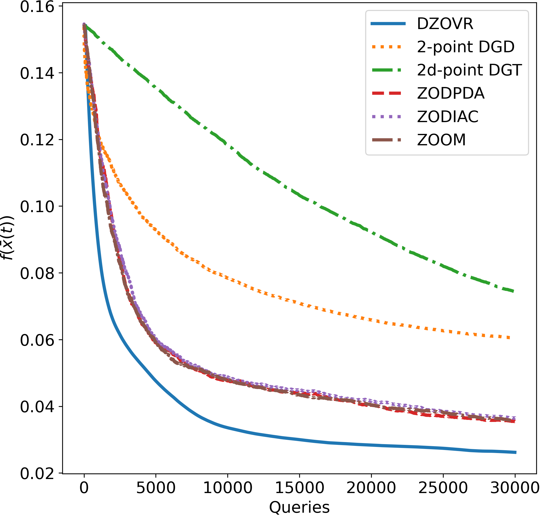
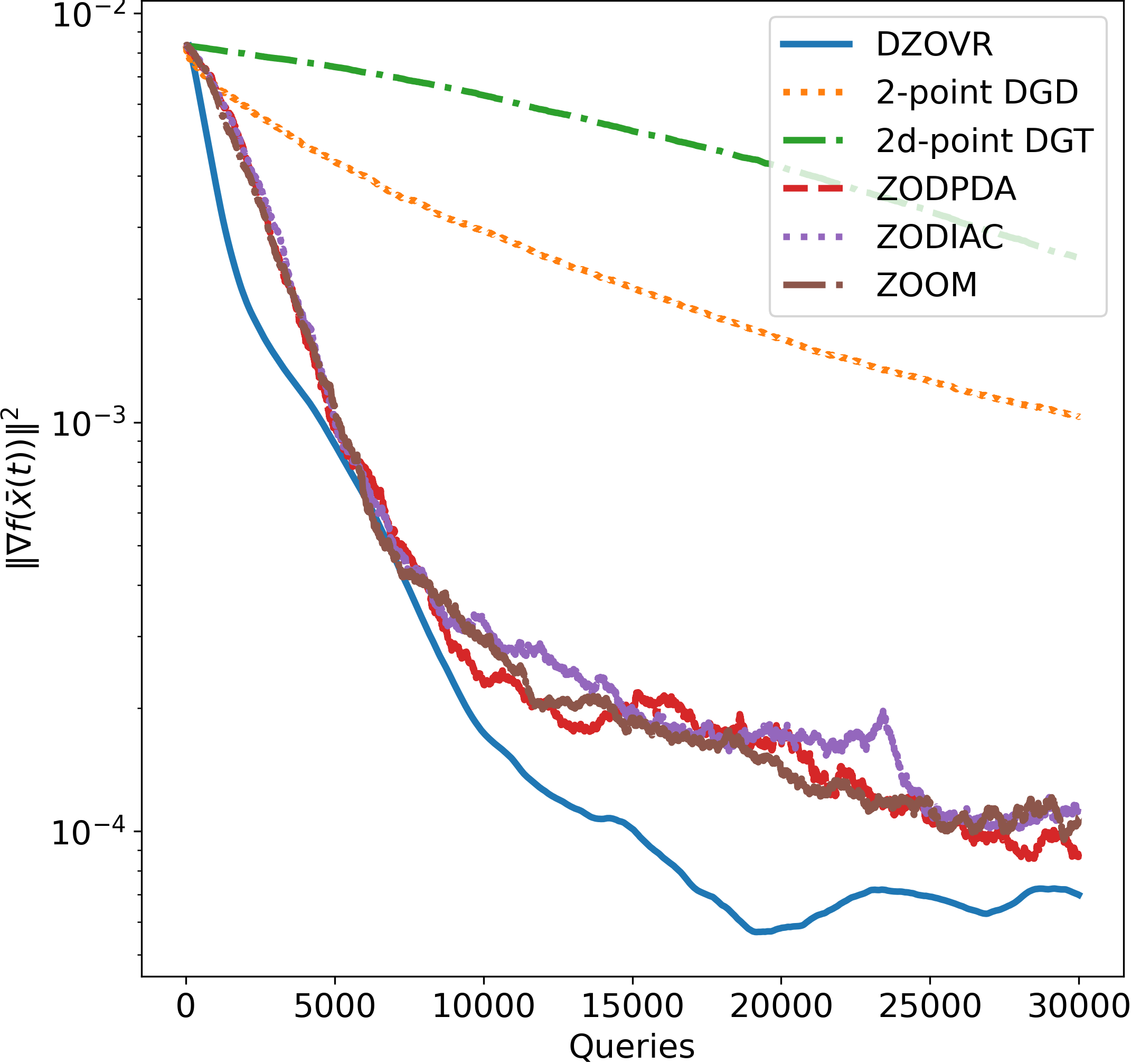
Figure 1: Comparison of the performance of different algorithms.

We first compare DZOVR with the following decentralized zeroth-order algorithms: 2-point DGD [28], 2d-point DGT [28], ZODPDA [38], ZODIAC [41], and ZOOM [42]. For 2-point DGD and 2d-point DGT, their step sizes are set as $0.1/k$ and 0.02 respectively. For the other three methods, the step size is set to 0.01. In DZOVR, we set $\beta=0.001$, $\alpha=0.05$ and $b_{0}=100$. Here the graph is created by first sampling $n$ points on $\mathbb{S}^{2}$ uniformly at random, and then linking pairs of points with spherical distances smaller than $\pi/4$ [28]. Metropolis-Hastings weights [30] are used to build $W$. The results of the numerical experiments are displayed in Figure 1. It’s worth noting that the horizontal axis in the figure represents queries because in zeroth-order algorithms, the focus is on achieving better results with as few queries as possible, rather than the number of iterations. Though DZOVR requires 4 queries in each iteration while the other methods require only 2 queries (except for 2d-point DGT), it still outperforms the other algorithms due to its faster convergence.

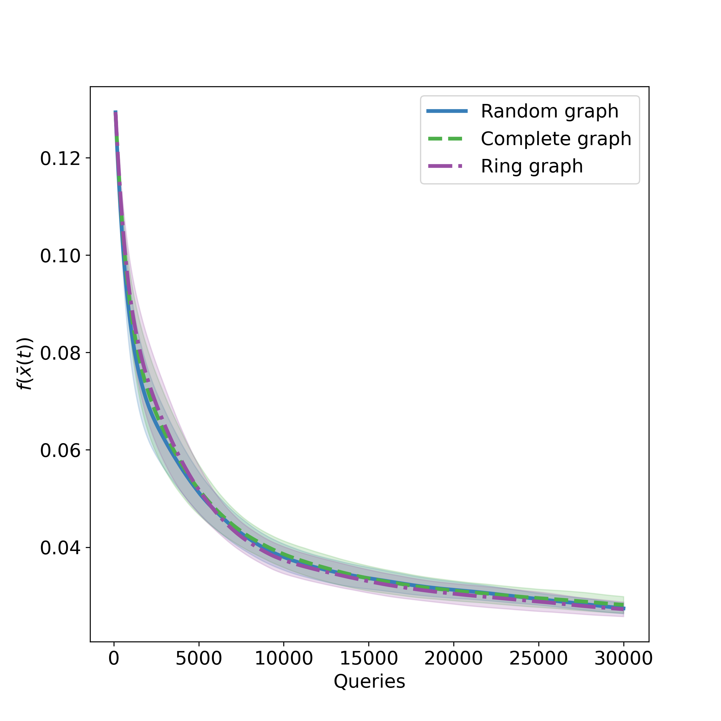
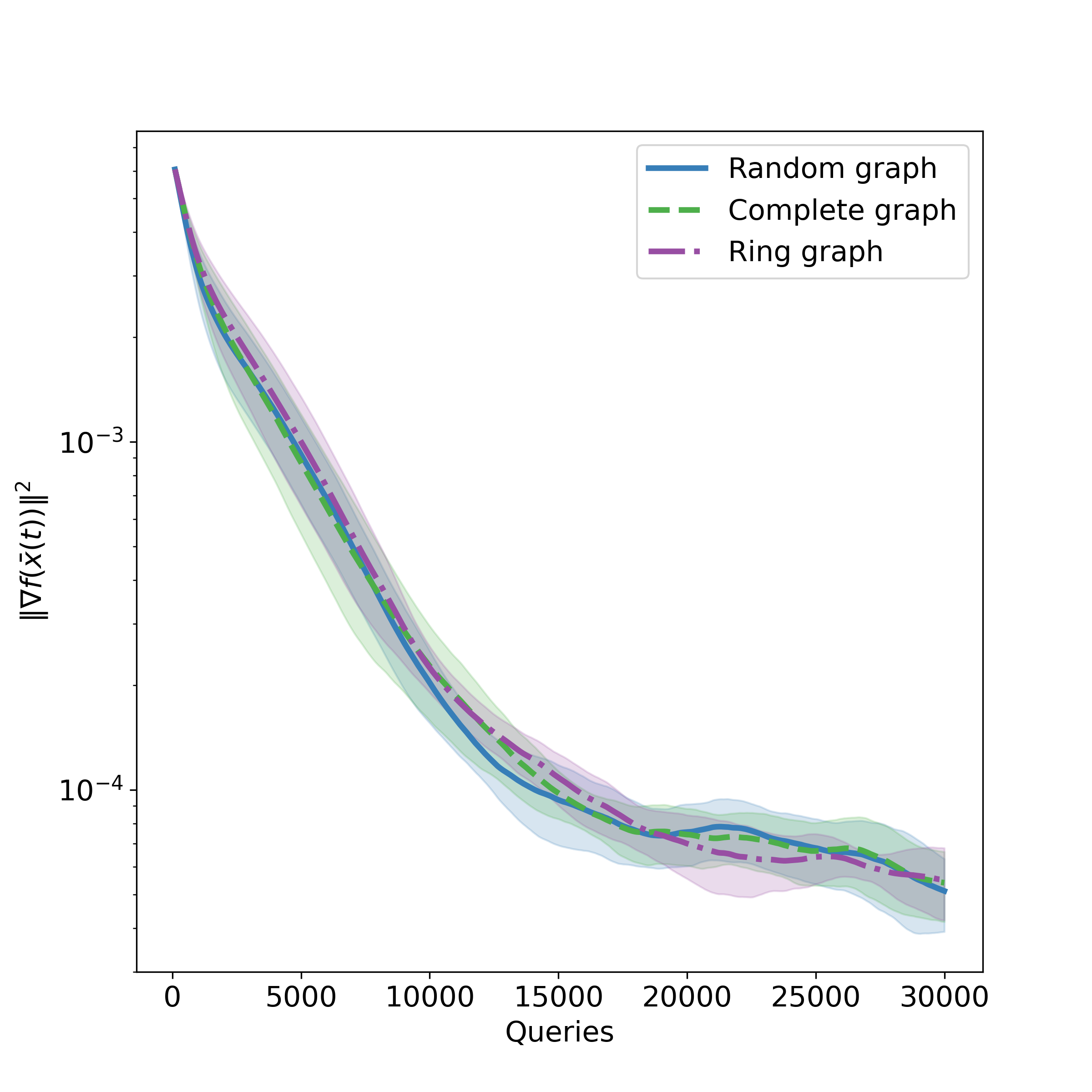
Figure 2: Performance of DZOVR under three different network topologies. The curves in the graph represent the average results out of 10 random trials, and the shaded areas represent the standard deviation.

To investigate the network-independent property of DZOVR, we conduct numerical experiments on three different network structures: the random graph mentioned above, the complete graph, and the ring graph. The mean objective function and gradient values as well as the standard deviations out of 10 repeated random tests are presented in Figure 2. It can be observed that DZOVR performs consistently well across the three network structures, indicating its network-independent property.

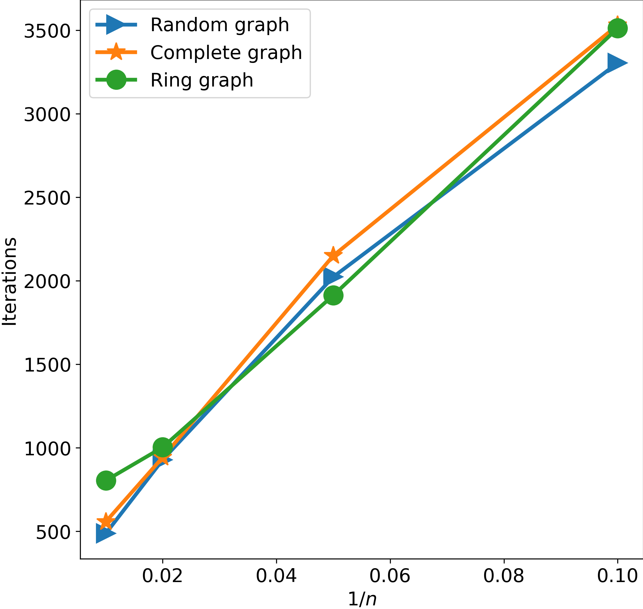
Figure 3: The linear speedup performance of DZOVR. The value of $n$ are $\{10,20,50,100\}$.

Regarding the linear speedup property of the algorithm, experiments are conducted with $n=\{10,20,50,100\}$, $\alpha=0.005n^{2/3}$ on the three aforementioned graphs. We record the number of iterations required for the squared norm of the gradient to be less than 0.001. The results are shown in Figure 3, where the $x$-axis represents $1/n$ and the $y$-axis represents the number of iterations required to achieve the specified accuracy. A desirable linear speedup can be observed from the figure.

4 Conclusion

We propose a decentralized zeroth-order variance reduced algorithm to mitigate the adverse effects of excessive variance in distributed zeroth-order optimization. It is proved that the algorithm convergences at a rate of $\mathcal{O}((d/{nK})^{2/3})$. Numerical experiments demonstrate its superior performance over state-of-the-art algorithms and its network-independent and linear speedup properties. Interesting directions for future works include analyzing the algorithm under the PL condition, accelerating the algorithm, or extending it to the non-smooth setting.

Appendix A Useful Lemmas

We first present several useful lemmas that will be utilized in the proof of Theorem 1.

Lemma 1 (Basic properties of 2-point estimator [28]).

• For a $L$-smooth function $f$,

  $$\left|\frac{f(x+tu)-f(x-tu)}{2t}-\langle\nabla f(x),u\rangle\right|\leq\frac{1}{2}tL\|u\|^{2}$$

  holds for any $x,u\in\mathbb{R}^{d}$.

• For the 2-point estimator $\hat{\nabla}f(x;u)=d\;\dfrac{f(x+tu)-f(x-tu)}{2t}\cdot u$, we have

  $$\mathbb{E}_{u\sim\mathcal{U}\left(\mathbb{S}_{d-1}\right)}[\hat{\nabla}f(x;u)]=\nabla f_{t}(x),$$

  where $f_{t}(x):=\mathbb{E}_{y\sim\mathcal{U}\left(\mathbb{B}_{d}\right)}[f(x+ty)]$. In addition, if $f$ is $L$-smooth, then $f_{t}$ is also $L$-smooth, and the following inequality holds:

  $$\left\|\nabla f(x)-\nabla f_{t}(x)\right\|\leq tL.$$

• For any deterministic $h\in\mathbb{R}^{d}$, we have

  $$\mathbb{E}_{z\sim\mathcal{U}\left(\mathbb{S}_{d-1}\right)}[d\cdot\langle h,z\rangle z]=h\quad\text{and}\quad\mathbb{E}_{z\sim\mathcal{U}\left(\mathbb{S}_{d-1}\right)}\left[d\cdot\langle h,z\rangle^{2}\right]=\|h\|^{2}.$$

For the sake of clarity, we define

$$\bar{m}^{k} =\frac{1}{n}\sum_{i=1}^{n}m_{i}^{k},$$

$$\nabla\bar{f}^{k} =\frac{1}{n}\sum_{i=1}^{n}\nabla f_{i}\left(x_{i}^{k}\right),$$

$$\hat{\nabla}\bar{f}\left(x^{k};u^{k},\xi^{k}\right) =\frac{1}{n}\sum_{i=1}^{n}\hat{\nabla}f_{i}\left(x_{i}^{k};u_{i}^{k},\xi_{i}^{k}\right),$$

$$\nabla f_{i,t_{k}}\left(x_{i}^{k}\right) =\mathbb{E}_{u\sim\mathcal{U}\left(\mathbb{S}_{d-1}\right)}\left[\hat{\nabla}f_{i}\left(x_{i}^{k}\right)\right],$$

$$\nabla f^{k} =\begin{bmatrix}\nabla f_{1}(x_{i}^{k})^{\top}&\cdots&\nabla f_{n}(x_{n}^{k})^{\top}\end{bmatrix}^{\top}\in\mathbb{R}^{nd}.$$

Lemma 2.

Suppose $\{x^{k},u^{k},\xi^{k}\}$ is a sequence generated by Algorithm 1. Under Assumption 2, 3, and 4, for any $k\geq 1$, one has

$$\mathbb{E}\left[\left\|\hat{\nabla}\bar{f}\left(x^{k};u^{k},\xi^{k}\right)\right\|^{2}\mid\mathcal{F}_{k}\right]\leq \frac{1}{2}L^{2}d^{2}t_{k}^{2}+\left(\frac{4dL^{2}\left(1+\sigma_{0}^{2}\right)}{n^{2}}+\frac{4L^{2}}{n}\right)\left\|x^{k}-1_{n}\otimes\bar{x}^{k}\right\|^{2}$$

$$+\left(\frac{8d}{n}\left(1+\sigma_{0}^{2}\right)\left(1+\sigma_{2}^{2}\right)+4\right)\left\|\nabla f\left(\bar{x}^{k}\right)\right\|^{2}+\frac{8d}{n}\left(1+\sigma_{0}^{2}\right)\sigma_{3}^{2}+\frac{2d}{n}\sigma_{1}^{2}.$$

Proof.

Conditioned on $\xi^{k}$ and $\mathcal{F}_{k}$, a straightforward computation yields that

$$\mathbb{E}_{u^{k}}\left\|\hat{\nabla}\bar{f}\left(x^{k};u^{k},\xi^{k}\right)\right\|^{2}$$

$$= \mathbb{E}_{u^{k}}\left\|\frac{1}{n}\sum_{i=1}^{n}d\frac{F_{i}\left(x_{i}^{k}+t_{k}u_{i}^{k};\xi_{i}^{k}\right)-F_{i}\left(x_{i}^{k}-t_{k}u_{i}^{k};\xi_{i}^{k}\right)}{2t_{k}}u_{i}^{k}\right\|^{2}$$

$$= \mathbb{E}_{u^{k}}\left\|\frac{d}{n}\sum_{i=1}^{n}\frac{F_{i}\left(x_{i}^{k}+t_{k}u_{i}^{k};\xi_{i}^{k}\right)-F_{i}\left(x_{i}^{k}-t_{k}u_{i}^{k};\xi_{i}^{k}\right)}{2t_{k}}u_{i}^{k}-\left\langle\nabla F_{i}\left(x_{i}^{k};\xi_{i}^{k}\right),u_{i}^{k}\right\rangle u_{i}^{k}+\left\langle\nabla F_{i}\left(x_{i}^{k};\xi_{i}^{k}\right),u_{i}^{k}\right\rangle u_{i}^{k}\right\|^{2}$$

$$\leq \frac{2d^{2}}{n}\sum_{i=1}^{n}\mathbb{E}_{u^{k}}\left\|\frac{F_{i}\left(x_{i}^{k}+t_{k}u_{i}^{k};\xi_{i}^{k}\right)-F_{i}\left(x_{i}^{k}-t_{k}u_{i}^{k};\xi_{i}^{k}\right)}{2t_{k}}u_{i}^{k}-\left\langle\nabla F_{i}\left(x_{i}^{k};\xi_{i}^{k}\right),u_{i}^{k}\right\rangle u_{i}^{k}\right\|^{2}$$

$$+2\mathbb{E}_{u^{k}}\left\|\frac{d}{n}\sum_{i=1}^{n}\left\langle\nabla F_{i}\left(x_{i}^{k};\xi_{i}^{k}\right),u_{i}^{k}\right\rangle u_{i}^{k}\right\|^{2}$$

$$\leq \frac{2d^{2}}{n}\cdot n\cdot\frac{1}{4}t_{k}^{2}L^{2}+\frac{2(d-1)}{n^{2}}\sum_{i=1}^{n}\left\|\nabla F_{i}\left(x_{i}^{k};\xi_{i}^{k}\right)\right\|^{2}+2\left\|\frac{1}{n}\sum_{i=1}^{n}\nabla F_{i}\left(x_{i}^{k};\xi_{i}^{k}\right)\right\|^{2},$$ (5)

where the last inequality is due to Lemma 1 and the fact that

$$\mathbb{E}_{u^{k}}\left\|\frac{d}{n}\sum_{i=1}^{n}\left\langle\nabla F_{i}\left(x_{i}^{k};\xi_{i}^{k}\right),u_{i}^{k}\right\rangle u_{i}^{k}\right\|^{2}\leq\frac{(d-1)}{n^{2}}\sum_{i=1}^{n}\left\|\nabla F_{i}\left(x_{i}^{k};\xi_{i}^{k}\right)\right\|^{2}+\left\|\frac{1}{n}\sum_{i=1}^{n}\nabla F_{i}\left(x_{i}^{k};\xi_{i}^{k}\right)\right\|^{2}.$$

The fact can be proved as follows:

$$\mathbb{E}_{u^{k}}\left\|\frac{d}{n}\sum_{i=1}^{n}\left\langle\nabla F_{i}\left(x_{i}^{k};\xi_{i}^{k}\right),u_{i}^{k}\right\rangle u_{i}^{k}\right\|^{2}$$

$$= \frac{d^{2}}{n^{2}}\mathbb{E}_{u^{k}}\left[\sum_{i=1}^{n}\left|\left\langle\nabla F_{i}\left(x_{i}^{k};\xi_{i}^{k}\right),u_{i}^{k}\right\rangle\right|^{2}+\sum_{i\neq j}\left\langle\nabla F_{i}\left(x_{i}^{k};\xi_{i}^{k}\right),u_{i}^{k}\right\rangle\left\langle\nabla F_{j}\left(x_{j}^{k};\xi_{j}^{k}\right),u_{j}^{k}\right\rangle\cdot\left\langle u_{i}^{k},u_{j}^{k}\right\rangle\right]$$

$$= \frac{d}{n^{2}}\sum_{i=1}^{n}\left\|\nabla F_{i}\left(x_{i}^{k};\xi_{i}^{k}\right)\right\|^{2}+\frac{1}{n^{2}}\sum_{i\neq j}\left\langle\nabla F_{i}\left(x_{i}^{k};\xi_{i}^{k}\right),\nabla F_{j}\left(x_{j}^{k};\xi_{j}^{k}\right)\right\rangle$$

$$= \frac{(d-1)}{n^{2}}\sum_{i=1}^{n}\left\|\nabla F_{i}\left(x_{i}^{k};\xi_{i}^{k}\right)\right\|^{2}+\frac{1}{n^{2}}\left\|\sum_{i=1}^{n}\nabla F_{i}\left(x_{i}^{k};\xi_{i}^{k}\right)\right\|^{2}$$

$$= \frac{(d-1)}{n^{2}}\sum_{i=1}^{n}\left\|\nabla F_{i}\left(x_{i}^{k};\xi_{i}^{k}\right)\right\|^{2}+\left\|\frac{1}{n}\sum_{i=1}^{n}\nabla F_{i}\left(x_{i}^{k};\xi_{i}^{k}\right)\right\|^{2},$$

where the second line is due to Lemma 1.

Thus, we have

$$\mathbb{E}\left[\left\|\hat{\nabla}\bar{f}\left(x^{k};u^{k},\xi^{k}\right)\right\|^{2}\mid\mathcal{F}_{k}\right]$$

$$= \mathbb{E}_{\xi^{k}}\mathbb{E}_{u^{k}}\left\|\hat{\nabla}\bar{f}\left(x^{k};u^{k},\xi^{k}\right)\right\|^{2}$$

$$\leq \frac{1}{2}L^{2}d^{2}t_{k}^{2}+\frac{2(d-1)}{n^{2}}\sum_{i=1}^{n}\mathbb{E}_{\xi^{k}}\left\|\nabla F_{i}\left(x_{i}^{k},\xi_{i}^{k}\right)\right\|^{2}+2\mathbb{E}_{\xi^{k}}\left\|\frac{1}{n}\sum_{i=1}^{n}\nabla F_{i}\left(x_{i}^{k},\xi_{i}^{k}\right)\right\|^{2}$$

$$\stackrel{{\scriptstyle(a)}}{{=}} \frac{1}{2}L^{2}d^{2}t_{k}^{2}+\frac{2(d-1)}{n^{2}}\sum_{i=1}^{n}\mathbb{E}_{\xi^{k}}\left\|\nabla F_{i}\left(x_{i}^{k},\xi_{i}^{k}\right)-\nabla f_{i}\left(x_{i}^{k}\right)\right\|^{2}+\frac{2(d-1)}{n^{2}}\sum_{i=1}^{n}\left\|\nabla f_{i}\left(x_{i}^{k}\right)\right\|^{2}$$

$$+2\mathbb{E}_{\xi^{k}}\|\frac{1}{n}\sum_{i=1}^{n}\nabla F_{i}\left(x_{i}^{k};\xi_{i}^{k}\right)-\frac{1}{n}\sum_{i=1}^{n}\nabla f_{i}\left(x_{i}^{k}\right)\left\|{}^{2}+2\right\|\frac{1}{n}\sum_{i=1}^{n}\nabla f_{i}\left(x_{i}^{k}\right)\|^{2}$$

$$\stackrel{{\scriptstyle(b)}}{{\leq}} \frac{1}{2}L^{2}d^{2}t_{k}^{2}+\frac{2(d-1)}{n^{2}}\sum_{i=1}^{n}\left(\sigma_{0}^{2}\left\|\nabla f_{i}\left(x_{i}^{k}\right)\right\|^{2}+\sigma_{1}^{2}\right)+\frac{2(d-1)}{n^{2}}\sum_{i=1}^{n}\left\|\nabla f_{i}\left(x_{i}^{k}\right)\right\|^{2}$$

$$+\frac{2}{n^{2}}\sigma_{0}^{2}\sum_{i=1}^{n}\left\|\nabla f_{i}\left(x_{i}^{k}\right)\right\|^{2}+\frac{2}{n}\sigma_{1}^{2}+2\left\|\frac{1}{n}\sum_{i=1}^{n}\nabla f_{i}\left(x_{i}^{k}\right)\right\|^{2}$$

$$\leq \frac{1}{2}L^{2}d^{2}t_{k}^{2}+\frac{2d}{n^{2}}\left(1+\sigma_{0}^{2}\right)\left\|\nabla f^{k}\right\|^{2}+\frac{2d}{n}\sigma_{1}^{2}+2\left\|\frac{1}{n}\sum_{i=1}^{n}\nabla f_{i}\left(x_{i}^{k}\right)\right\|^{2}$$

$$\stackrel{{\scriptstyle(c)}}{{\leq}} \frac{1}{2}L^{2}d^{2}t_{k}^{2}+\frac{2d}{n^{2}}\left(1+\sigma_{0}^{2}\right)\left(2L^{2}\left\|x^{k}-1_{n}\otimes\bar{x}^{k}\right\|^{2}+4n\left(1+\sigma_{2}^{2}\right)\left\|\nabla f\left(\bar{x}^{k}\right)\right\|^{2}+4n\sigma_{3}^{2}\right)$$

$$+4\left\|\nabla f\left(\bar{x}^{k}\right)\right\|^{2}+\frac{4L^{2}}{n}\left\|x^{k}-1_{n}\otimes\bar{x}^{k}\right\|^{2}+\frac{2d}{n}\sigma_{1}^{2}$$

$$= \frac{1}{2}L^{2}d^{2}t_{k}^{2}+\left(\frac{4dL^{2}\left(1+\sigma_{0}^{2}\right)}{n^{2}}+\frac{4L^{2}}{n}\right)\left\|x^{k}-1_{n}\otimes\bar{x}^{k}\right\|^{2}$$

$$+\left(\frac{8d}{n}\left(1+\sigma_{0}^{2}\right)\left(1+\sigma_{2}^{2}\right)+4\right)\left\|\nabla f\left(\bar{x}^{k}\right)\right\|^{2}+\frac{8d}{n}\left(1+\sigma_{0}^{2}\right)\sigma_{3}^{2}+\frac{2d}{n}\sigma_{1}^{2},$$

where step (a) and step (b) follow from Assumption 3, step (c) uses the fact

$$\|\nabla f^{k}\|_{2}^{2} \leq 2L^{2}\|x^{k}-1_{n}\otimes\bar{x}^{k}\|^{2}+4n(1+\sigma_{2}^{2})\|\nabla f(\bar{x}^{k})\|^{2}+4n\sigma_{3}^{2},$$

$$\left\|\frac{1}{n}\sum_{i=1}^{n}\nabla f_{i}(x_{i}^{k})\right\|^{2} \leq\frac{2L^{2}}{n}\|x^{k}-1_{n}\otimes\bar{x}^{k}\|^{2}+2\left\|\nabla f(\bar{x}^{k})\right\|^{2}.$$ (6)

Moreover, the fact used in step (c) can be proved as follows:

$$\|\nabla f^{k}\|^{2} =\sum_{i=1}^{n}\|\nabla f_{i}(x_{i}^{k})\|^{2}$$

$$\leq 2\sum_{i=1}^{n}\|\nabla f_{i}(x_{i}^{k})-\nabla f_{i}(\bar{x}^{k})\|^{2}+2\sum_{i=1}^{n}\|\nabla f_{i}(\bar{x}^{k})\|^{2}$$

$$\leq 2\sum_{i=1}^{n}\|\nabla f_{i}(x_{i}^{k})-\nabla f_{i}(\bar{x}^{k})\|^{2}+4\sum_{i=1}^{n}\|\nabla f_{i}(\bar{x}^{k})-\nabla f(\bar{x}^{k})\|^{2}+4\sum_{i=1}^{n}\|\nabla f(\bar{x}^{k})\|^{2}$$

$$\stackrel{{\scriptstyle(a)}}{{\leq}}2L^{2}\sum_{i=1}^{n}\|x_{i}^{k}-\bar{x}^{k}\|^{2}+4\sum_{i=1}^{n}\left(\sigma_{2}^{2}\|\nabla f(\bar{x})\|^{2}+\sigma_{3}^{2}\right)+4\sum_{i=1}^{n}\|\nabla f(\bar{x}^{k})\|^{2}$$

$$=2L^{2}\|x^{k}-1_{n}\otimes\bar{x}^{k}\|^{2}+4n(1+\sigma_{2}^{2})\|\nabla f(\bar{x}^{k})\|^{2}+4n\sigma_{3}^{2},$$

where step (a) follows from Assumption 2 and Assumption 4. Using the same argument as above, one can obtain

$$\left\|\frac{1}{n}\sum_{i=1}^{n}\nabla f_{i}(x_{i}^{k})\right\|^{2} \leq 2\left\|\frac{1}{n}\sum_{i=1}^{n}\nabla f_{i}(x_{i}^{k})-\nabla f(\bar{x}^{k})\right\|^{2}+2\|\nabla f(\bar{x}^{k})\|^{2}$$

$$=2\left\|\frac{1}{n}\sum_{i=1}^{n}\left(\nabla f_{i}(x_{i}^{k})-\nabla f_{i}(\bar{x}^{k})\right)\right\|^{2}+2\|\nabla f(\bar{x}^{k})\|^{2}$$

$$\stackrel{{\scriptstyle(a)}}{{\leq}}\frac{2}{n}\sum_{i=1}^{n}\|\nabla f_{i}(x_{i}^{k})-\nabla f_{i}(\bar{x}^{k})\|^{2}+2\left\|\nabla f(\bar{x}^{k})\right\|^{2}$$

$$\leq\frac{2L^{2}}{n}\sum_{i=1}^{n}\|x_{i}^{k}-\bar{x}^{k}\|^{2}+2\left\|\nabla f(\bar{x}^{k})\right\|^{2}$$

$$=\frac{2L^{2}}{n}\|x^{k}-1_{n}\otimes\bar{x}^{k}\|^{2}+2\left\|\nabla f(\bar{x}^{k})\right\|^{2},$$

where step (a) is due to the Jensen’s inequality. ∎

Lemma 3.

Consider the same setup as stated in Lemma 2. One has

$$\mathbb{E}\left[\left\|\hat{\nabla}f\left(x^{k};u^{k},\xi^{k}\right)\right\|^{2}\mid\mathcal{F}_{k}\right]\leq \frac{1}{2}nd^{2}L^{2}t_{k}^{2}+6dL^{2}\left(1+\sigma_{0}^{2}\right)\left\|x^{k}-1_{n}\otimes\bar{x}^{k}\right\|^{2}$$

$$\quad+6nd\left(1+\sigma_{0}^{2}\right)\left(1+\sigma_{2}^{2}\right)\left\|\nabla f\left(\bar{x}^{k}\right)\right\|^{2}+6nd\left(1+\sigma_{0}^{2}\right)\sigma_{3}^{2}+2nd\sigma_{1}^{2}.$$

Proof.

Recall the definition of $\hat{\nabla}f\left(x^{k};u^{k},\xi^{k}\right)$ in (4). A direct computation yields that

$$\mathbb{E}\left[\left\|\hat{\nabla}f\left(x^{k};u^{k},\xi^{k}\right)\right\|^{2}\mid\mathcal{F}_{k}\right]$$

$$= \mathbb{E}_{\xi^{k}}\mathbb{E}_{u^{k}}\left[\sum_{i=1}^{n}\left\|\hat{\nabla}f_{i}\left(x_{i}^{k};u_{i}^{k},\xi_{i}^{k}\right)\right\|^{2}\right]$$

$$= \mathbb{E}_{\xi^{k}}\mathbb{E}_{u^{k}}\sum_{i=1}^{n}\left\|d\frac{F_{i}\left(x_{i}^{k}+t_{k}u_{i}^{k};\xi_{i}^{k}\right)-F_{i}\left(x_{i}^{k}-t_{k}u_{i}^{k};\xi_{i}^{k}\right)}{2t_{k}}u_{i}^{k}\right\|^{2}$$

$$= \mathbb{E}_{\xi^{k}}\mathbb{E}_{u^{k}}\sum_{i=1}^{n}\left\|d\frac{F_{i}\left(x_{i}^{k}+t_{k}u_{i}^{k};\xi_{i}^{k}\right)-F_{i}\left(x_{i}^{k}-t_{k}u_{i}^{k};\xi_{i}^{k}\right)}{2t_{k}}u_{i}^{k}-d\left\langle\nabla F_{i}\left(x_{i}^{k};\xi_{i}^{k}\right),u_{i}^{k}\right\rangle u_{i}^{k}+d\left\langle\nabla F_{i}\left(x_{i}^{k};\xi_{i}^{k}\right),u_{i}^{k}\right\rangle u_{i}^{k}\right\|^{2}$$

$$\leq 2d^{2}\mathbb{E}_{\xi^{k}}\mathbb{E}_{u^{k}}\sum_{i=1}^{n}\left\|\frac{F_{i}\left(x_{i}^{k}+t_{k}u_{i}^{k};\xi_{i}^{k}\right)-F_{i}\left(x_{i}^{k}-t_{k}u_{i}^{k};\xi_{i}^{k}\right)}{2t_{k}}u_{i}^{k}-\left\langle\nabla F_{i}\left(x_{i}^{k};\xi_{i}^{k}\right),u_{i}^{k}\right\rangle u_{i}^{k}\right\|^{2}$$

$$+2\mathbb{E}_{\xi^{k}}\mathbb{E}_{u^{k}}\sum_{i=1}^{n}\|d\left\langle\nabla F_{i}\left(x_{i}^{k};\xi_{i}^{k}\right),u_{i}^{k}\right\rangle u_{i}^{k}\|^{2}$$

$$\stackrel{{\scriptstyle(a)}}{{\leq}} 2d^{2}\cdot\frac{1}{4}nL^{2}t_{k}^{2}+2d\sum_{i=1}^{n}\mathbb{E}_{\xi^{k}}\left\|\nabla F_{i}\left(x_{i}^{k};\xi_{i}^{k}\right)\right\|^{2}$$

$$\stackrel{{\scriptstyle(b)}}{{=}} \frac{1}{2}nd^{2}L^{2}t_{k}^{2}+2d\sum_{i=1}^{n}\left\|\nabla f_{i}\left(x_{i}^{k}\right)\right\|^{2}+2d\sum_{i=1}^{n}\left\|\nabla F_{i}\left(x_{i}^{k};\xi_{i}^{k}\right)-\nabla f_{i}\left(x_{i}^{k}\right)\right\|^{2}$$

$$\stackrel{{\scriptstyle(c)}}{{\leq}} \frac{1}{2}nd^{2}L^{2}t_{k}^{2}+2d\sum_{i=1}^{n}\left\|\nabla f_{i}\left(x_{i}^{k}\right)\right\|^{2}+2d\sum_{i=1}^{n}\left(\sigma_{0}^{2}\|\nabla f_{i}(x_{i}^{k})\|^{2}+\sigma_{1}^{2}\right)$$

$$= \frac{1}{2}nd^{2}L^{2}t_{k}^{2}+2d\left(1+\sigma_{0}^{2}\right)\sum_{i=1}^{n}\left\|\nabla f_{i}\left(x_{i}^{k}\right)\right\|^{2}+2nd\sigma_{1}^{2},$$ (7)

where step (a) is due to Lemma 1, step (b) uses the fact that $\mathbb{E}_{\xi_{i}^{k}}\left[\langle\nabla F_{i}(x_{i}^{k};\xi_{i}^{k})-\nabla f_{i}(x_{i}^{k}),\nabla f_{i}(x_{i}^{k})\rangle\right]=0$, and step (c) follows from Assumption 3. Moreover, one can show that

$$\sum_{i=1}^{n}\left\|\nabla f_{i}\left(x_{i}^{k}\right)\right\|^{2} =\sum_{i=1}^{n}\left\|\nabla f_{i}\left(x_{i}^{k}\right)-\nabla f_{i}\left(\bar{x}^{k}\right)+\nabla f_{i}\left(\bar{x}^{k}\right)-\nabla f\left(\bar{x}^{k}\right)+\nabla f\left(\bar{x}^{k}\right)\right\|^{2}$$

$$\leq 3\sum_{i=1}^{n}\left\|\nabla f_{i}\left(x_{i}^{k}\right)-\nabla f_{i}\left(\bar{x}^{k}\right)\right\|^{2}+3\sum_{i=1}^{n}\left\|\nabla f_{i}\left(\bar{x}^{k}\right)-\nabla f\left(\bar{x}^{k}\right)\right\|^{2}+3n\left\|\nabla f\left(\bar{x}^{k}\right)\right\|^{2}$$

$$\leq 3L^{2}\left\|x^{k}-1_{n}\otimes\bar{x}^{k}\right\|^{2}+3\sum_{i=1}^{n}\left(\sigma_{2}^{2}\left\|\nabla f\left(\bar{x}^{k}\right)\right\|^{2}+\sigma_{3}^{2}\right)+3n\left\|\nabla f\left(\bar{x}^{k}\right)\right\|^{2}$$

$$=3L^{2}\left\|x^{k}-1_{n}\otimes\bar{x}^{k}\right\|^{2}+3n\left(1+\sigma_{2}^{2}\right)\left\|\nabla f\left(\bar{x}^{k}\right)\right\|^{2}+3n\sigma_{3}^{2},$$ (8)

where the third line is due to Assumption 2 and Assumption 4. Plugging (8) into (7), we get

$$\mathbb{E}\left[\left\|\hat{\nabla}f\left(x^{k};u^{k},\xi^{k}\right)\right\|^{2}\mid\mathcal{F}_{k}\right]\leq \frac{1}{2}nd^{2}L^{2}t_{k}^{2}+6dL^{2}\left(1+\sigma_{0}^{2}\right)\left\|x^{k}-1_{n}\otimes\bar{x}^{k}\right\|^{2}$$

$$\quad+6nd\left(1+\sigma_{0}^{2}\right)\left(1+\sigma_{2}^{2}\right)\left\|\nabla f\left(\bar{x}^{k}\right)\right\|^{2}+6nd\left(1+\sigma_{0}^{2}\right)\sigma_{3}^{2}+2nd\sigma_{1}^{2}.$$

∎

Lemma 4.

Consider the sequence $\left\{m^{k}\right\}$ generated by Algorithm 1. Under Assumption 2, 3, and 4, for $k\geq 1$, we have

$$\mathbb{E}\left\|\bar{m}^{k}-\nabla\bar{f}^{k}\right\|^{2}\leq \;\frac{1+(1-\beta)^{2}}{2}\mathbb{E}\left\|\bar{m}^{k-1}-\nabla\bar{f}^{k-1}\right\|^{2}+\left(\frac{32\beta^{2}d}{n}\left(1+\sigma_{0}^{2}\right)\left(1+\sigma_{2}^{2}\right)+24\beta^{2}\right)\mathbb{E}\left\|\nabla f\left(\bar{x}^{k}\right)\right\|^{2}$$

$$+\frac{36\alpha^{2}(1-\beta)^{2}dL^{2}}{n}\mathbb{E}\left\|\bar{m}^{k-1}\right\|^{2}+\frac{36(1-\beta)^{2}dL^{2}}{n^{2}}\mathbb{E}\left\|x^{k-1}-1_{n}\otimes\bar{x}^{k-1}\right\|^{2}$$

$$+\left(\frac{16\beta^{2}dL^{2}\left(1+\sigma_{0}^{2}\right)}{n^{2}}+\frac{24\beta^{2}L^{2}}{n}+\frac{36(1-\beta)^{2}dL^{2}}{n^{2}}\right)\mathbb{E}\left\|x^{k}-1_{n}\otimes\bar{x}^{k}\right\|^{2}$$

$$+\left(2\beta^{2}L^{2}d^{2}+16(1-\beta)^{2}L^{2}+\frac{6(1-\beta)^{2}d^{2}L^{2}}{n}+\frac{2(1-\beta)^{2}(2-\beta)L^{2}}{\beta}\right)t_{k}^{2}$$

$$+\frac{8\beta^{2}d}{n}\sigma_{1}^{2}+\frac{32\beta^{2}d}{n}\left(1+\sigma_{0}^{2}\right)\sigma_{3}^{2}.$$

Proof.

Following the momentum update in Algorithm 1, we have

$$\bar{m}^{k}-\nabla\bar{f}^{k} =(1-\beta)(\bar{m}^{k-1}-\nabla\bar{f}^{k-1})+\beta\underbrace{\left(\frac{1}{n}\sum_{i=1}^{n}\hat{\nabla}f_{i}(x_{i}^{k};u_{i}^{k},\xi_{i}^{k})-\nabla\bar{f}^{k}\right)}_{:=\bar{v}_{k}}$$

$$\quad+(1-\beta)\underbrace{\left(\frac{1}{n}\sum_{i=1}^{n}\left(\hat{\nabla}f_{i}\left(x_{i}^{k};u_{i}^{k},\xi_{i}^{k}\right)-\hat{\nabla}f_{i}\left(x_{i}^{k-1};u_{i}^{k},\xi_{i}^{k}\right)\right)-\left(\nabla\bar{f}^{k}-\nabla\bar{f}^{k-1}\right)\right)}_{:=\bar{r}_{k}}.$$

Thus it can be seen that

$$\mathbb{E}\left[\left\|\bar{m}^{k}-\nabla\bar{f}^{k}\right\|^{2}\mid\mathcal{F}_{k}\right]= \mathbb{E}\left[\left\|(1-\beta)\left(\bar{m}^{k-1}-\nabla\bar{f}^{k-1}\right)+\beta\bar{v}_{k}+(1-\beta)\bar{r}_{k}\right\|^{2}\mid\mathcal{F}_{k}\right]$$

$$= \;(1-\beta)^{2}\mathbb{E}\left[\left\|\bar{m}^{k-1}-\nabla\bar{f}^{k-1}\right\|^{2}\mid\mathcal{F}_{k}\right]+\mathbb{E}\left[\left\|\beta\bar{v}_{k}+(1-\beta)\bar{r}_{k}\right\|^{2}\mid\mathcal{F}_{k}\right]$$

$$+2\mathbb{E}\left[\left\langle\beta\bar{v}_{k}+(1-\beta)\bar{r}_{k},(1-\beta)\left(\bar{m}^{k-1}-\nabla\bar{f}^{k-1}\right)\right\rangle\mid\mathcal{F}_{k}\right].$$ (9)

Notice that

$$2\mathbb{E}\left[\left\langle\beta\bar{v}_{k}+(1-\beta)\bar{r}_{k},(1-\beta)\left(\bar{m}^{k-1}-\nabla\bar{f}^{k-1}\right)\right\rangle\mid\mathcal{F}_{k}\right]$$

$$= \;2\mathbb{E}_{u^{k},\xi^{k}}\left\langle\beta\bar{v}_{k}+(1-\beta)\bar{r}_{k},(1-\beta)\left(\bar{m}^{k-1}-\nabla\bar{f}^{k-1}\right)\right\rangle$$

$$\stackrel{{\scriptstyle(a)}}{{=}} \;2\left\langle\frac{1}{n}\sum_{i=1}^{n}\left(\nabla f_{i,t_{k}}\left(x_{i}^{k}\right)-\nabla f_{i}\left(x_{i}^{k}\right)\right)-(1-\beta)\frac{1}{n}\sum_{i=1}^{n}\left(\nabla f_{i,t_{k}}\left(x_{i}^{k-1}\right)-\nabla f_{i}\left(x_{i}^{k-1}\right)\right),(1-\beta)\left(\bar{m}^{k-1}-\nabla\bar{f}^{k-1}\right)\right\rangle$$

$$\leq \;2\left\|\frac{1}{n}\sum_{i=1}^{n}\left(\nabla f_{i,t_{k}}\left(x_{i}^{k}\right)-\nabla f_{i}\left(x_{i}^{k}\right)\right)-(1-\beta)\frac{1}{n}\sum_{i=1}^{n}\left(\nabla f_{i,t_{k}}\left(x_{i}^{k-1}\right)-\nabla f_{i}\left(x_{i}^{k-1}\right)\right)\right\|\cdot\left\|(1-\beta)\left(\bar{m}^{k-1}-\nabla\bar{f}^{k-1}\right)\right\|$$

$$\stackrel{{\scriptstyle(b)}}{{\leq}} \;\frac{2(1-\beta)^{2}}{\beta(2-\beta)}\left\|\frac{1}{n}\sum_{i=1}^{n}\left(f_{i,t_{k}}\left(x_{i}^{k}\right)-\nabla f_{i}\left(x_{i}^{k}\right)\right)-(1-\beta)\frac{1}{n}\sum_{i=1}^{n}\left(\nabla f_{i,t_{k}}\left(x_{i}^{k-1}\right)-\nabla f_{i}\left(x_{i}^{k-1}\right)\right)\right\|^{2}$$

$$+\frac{\beta(2-\beta)}{2}\left\|\bar{m}^{k-1}-\nabla\bar{f}^{k-1}\right\|^{2}$$

$$\stackrel{{\scriptstyle(c)}}{{\leq}} \;\frac{\beta(2-\beta)}{2}\left\|\bar{m}^{k-1}-\nabla\bar{f}^{k-1}\right\|^{2}+\frac{2(1-\beta)^{2}(2-\beta)}{\beta}L^{2}t_{k}^{2},$$ (10)

where step (a) is due to Lemma 1, i.e., $\mathbb{E}_{u^{k}_{i},\xi_{i}^{k}}\left[\hat{\nabla}f_{i}(x_{i}^{k};u_{i}^{k},\xi_{i}^{k})\right]=\nabla f_{i,t_{k}}(x_{i}^{k})$, step (b) uses the elementary inequality that $2xy\leq\frac{1}{a}x^{2}+ay^{2}$ with $a=\beta(2-\beta)/2$, and step (c) follows from the fact that

$$\left\|\frac{1}{n}\sum_{i=1}^{n}\left(\nabla f_{i,t_{k}}\left(x_{i}^{k}\right)-\nabla f_{i}\left(x_{i}^{k}\right)\right)-(1-\beta)\frac{1}{n}\sum_{i=1}^{n}\left(\nabla f_{i,t_{k}}\left(x_{i}^{k-1}\right)-\nabla f_{i}\left(x_{i}^{k-1}\right)\right)\right\|\leq(2-\beta)Lt_{k}.$$

Moreover, the fact used in step (c) can be proved as follows:

$$\left\|\frac{1}{n}\sum_{i=1}^{n}\left(\nabla f_{i,t_{k}}\left(x_{i}^{k}\right)-\nabla f_{i}\left(x_{i}^{k}\right)\right)-(1-\beta)\frac{1}{n}\sum_{i=1}^{n}\left(\nabla f_{i,t_{k}}\left(x_{i}^{k-1}\right)-\nabla f_{i}\left(x_{i}^{k-1}\right)\right)\right\|$$

$$\leq \;\frac{1}{n}\sum_{i=1}^{n}\left\|\nabla f_{i,t_{k}}\left(x_{i}^{k}\right)-\nabla f_{i}\left(x_{i}^{k}\right)\right\|+(1-\beta)\frac{1}{n}\sum_{i=1}^{n}\left\|\nabla f_{i,t_{k}}\left(x_{i}^{k-1}\right)-\nabla f_{i}\left(x_{i}^{k-1}\right)\right\|$$

$$\leq \;Lt_{k}+(1-\beta)Lt_{k}$$

$$= \;(2-\beta)Lt_{k},$$

where third line is due to Lemma 1.

Substituting equation (10) into equation (9) yields

$$\mathbb{E}\left[\left\|\bar{m}^{k}-\nabla\bar{f}^{k}\right\|^{2}\mid\mathcal{F}_{k}\right]$$

$$\leq \frac{1+(1-\beta)^{2}}{2}\left\|\bar{m}^{k-1}-\nabla\bar{f}^{k-1}\right\|^{2}+\mathbb{E}\left[\left\|\beta\bar{v}_{k}+(1-\beta)\bar{r}_{k}\right\|^{2}\mid\mathcal{F}_{k}\right]+\frac{2(1-\beta)^{2}(2-\beta)}{\beta}L^{2}t_{k}^{2}$$

$$\leq \;\frac{1+(1-\beta)^{2}}{2}\left\|\bar{m}^{k-1}-\nabla\bar{f}^{k-1}\right\|^{2}+2\beta^{2}\mathbb{E}\left[\left\|\bar{v}_{k}\right\|^{2}\mid\mathcal{F}_{k}\right]+2(1-\beta)^{2}\mathbb{E}\left[\left\|\bar{r}_{k}\right\|^{2}\mid\mathcal{F}_{k}\right]$$

$$+\frac{2(1-\beta)^{2}(2-\beta)}{\beta}L^{2}t_{k}^{2}.$$ (11)

Next, we bound $\mathbb{E}\left[\left\|\bar{v}_{k}\right\|^{2}\mid\mathcal{F}_{k}\right]$ and $\mathbb{E}\left[\left\|\bar{r}_{k}\right\|^{2}\mid\mathcal{F}_{k}\right]$, respectively. For the first term, a simple calculation yields that

$$\mathbb{E}\left[\left\|\bar{v}_{k}\right\|^{2}\mid\mathcal{F}_{k}\right]= \;\mathbb{E}\left[\left\|\frac{1}{n}\sum_{i=1}^{n}\hat{\nabla}f_{i}\left(x_{i}^{k},u_{i}^{k},z_{i}^{k}\right)-\nabla\bar{f}^{k}\right\|^{2}\mid\mathcal{F}_{k}\right]$$

$$= \;\mathbb{E}\left[\left\|\hat{\nabla}\bar{f}\left(x^{k};u^{k},\xi^{k}\right)-\nabla\bar{f}^{k}\right\|^{2}\mid\mathcal{F}_{k}\right]$$

$$\leq \;2\mathbb{E}\left[\left\|\hat{\nabla}\bar{f}\left(x^{k};u^{k},\xi^{k}\right)\right\|^{2}\mid\mathcal{F}_{k}\right]+2\mathbb{E}\left[\left\|\nabla\bar{f}^{k}\right\|^{2}\mid\mathcal{F}_{k}\right]$$

$$\leq \;L^{2}d^{2}t_{k}^{2}+\left(\frac{8dL^{2}\left(1+\sigma_{0}^{2}\right)}{n^{2}}+\frac{12L^{2}}{n}\right)\left\|x^{k}-1_{n}\otimes\bar{x}^{k}\right\|^{2}$$

$$+\left(\frac{16d}{n}\left(1+\sigma_{0}^{2}\right)\left(1+\sigma_{2}^{2}\right)+12\right)\left\|\nabla f\left(\bar{x}^{k}\right)\right\|^{2}+\frac{16d}{n}\left(1+\sigma_{0}^{2}\right)\sigma_{3}^{2}+\frac{4d}{n}\sigma_{1}^{2},$$ (12)

where the last line follows from Lemma 2 and (6). Finally, we turn to control $\mathbb{E}\left[\left\|\bar{r}_{k}\right\|^{2}\mid\mathcal{F}_{k}\right]$. A direct computation yields that

$$\mathbb{E}_{u^{k},\xi^{k}}\left\|\hat{\nabla}f_{i}\left(x_{i}^{k};u_{i}^{k},\xi_{i}^{k}\right)-\hat{\nabla}f_{i}\left(x_{i}^{k-1};u_{i}^{k},\xi_{i}^{k}\right)\right\|^{2}$$

$$\leq \;3\mathbb{E}_{\xi^{k}}E_{u^{k}}\left\|d\frac{F_{i}\left(x_{i}^{k}+t_{k}u_{i}^{k};\xi_{i}^{k}\right)-F_{i}\left(x_{i}^{k}-t_{k}u_{i}^{k};\xi_{i}^{k}\right)}{2t_{k}}u_{i}^{k}-d\left\langle\nabla F_{i}\left(x_{i}^{k};\xi_{i}^{k}\right),u_{i}^{k}\right\rangle u_{i}^{k}\right\|^{2}$$

$$+3\mathbb{E}_{\xi^{k}}E_{u^{k}}\left\|d\frac{F_{i}\left(x_{i}^{k-1}+t_{k}u_{i}^{k};\xi_{i}^{k}\right)-F_{i}\left(x_{i}^{k-1}-t_{k}u_{i}^{k};\xi_{i}^{k}\right)}{2t_{k}}u_{i}^{k}-d\left\langle\nabla F_{i}\left(x_{i}^{k-1};\xi_{i}^{k}\right),u_{i}^{k}\right\rangle u_{i}^{k}\right\|^{2}$$

$$+3\mathbb{E}_{\xi^{k}}E_{u^{k}}\left\|d\left\langle\nabla F_{i}\left(x_{i}^{k};\xi_{i}^{k}\right)-\nabla F_{i}\left(x_{i}^{k-1};\xi_{i}^{k}\right),u_{i}^{k}\right\rangle u_{i}^{k}\right\|^{2}$$

$$\stackrel{{\scriptstyle(a)}}{{\leq}} \;\frac{3}{2}d^{2}L^{2}t_{k}^{2}+3dE_{\xi^{k}}\left\|\nabla F_{i}\left(x_{i}^{k};\xi_{i}^{k}\right)-\nabla F_{i}\left(x_{i}^{k-1};\xi_{i}^{k}\right)\right\|^{2}$$

$$\stackrel{{\scriptstyle(b)}}{{\leq}} \;\frac{3}{2}d^{2}L^{2}t_{k}^{2}+3dL^{2}\left\|x_{i}^{k}-x_{i}^{k-1}\right\|^{2},$$ (13)

where step (a) is due to Lemma 1 and step (b) follows from the $L$-smoothness of $F_{i}\left(\cdot;\xi_{i}^{k}\right)$. Thus it can be seen that

$$\mathbb{E}\left[\left\|\bar{r}_{k}\right\|^{2}\mid\mathcal{F}_{k}\right]$$

$$= \;\mathbb{E}\left[\left\|\frac{1}{n}\sum_{i=1}^{n}\left(\hat{\nabla}f_{i}\left(x_{i}^{k};u_{i}^{k},\xi_{i}^{k}\right)-\hat{\nabla}f_{i}\left(x_{i}^{k-1};u_{i}^{k},\xi_{i}^{k}\right)+\nabla f_{i}\left(x_{i}^{k-1}\right)-\nabla f_{i}\left(x_{i}^{k}\right)\right)\right\|^{2}\mid\mathcal{F}_{k}\right]$$

$$= \;\mathbb{E}_{u^{k},\xi^{k}}\Bigg{\|}\frac{1}{n}\sum_{i=1}^{n}{\left[\hat{\nabla}f_{i}\left(x_{i}^{k};u_{i}^{k},\xi_{i}^{k}\right)-\hat{\nabla}f_{i}\left(x_{i}^{k-1};u_{i}^{k},\xi_{i}^{k}\right)-\left(\nabla f_{i,t_{k}}\left(x_{i}^{k}\right)-\nabla f_{i,t_{k}}\left(x_{i}^{k-1}\right)\right)\right.}$$

$$\left.+\left(\nabla f_{i,t_{k}}\left(x_{i}^{k}\right)-\nabla f_{i,t_{k}}\left(x_{i}^{k-1}\right)\right)-\left(\nabla f_{i}\left(x_{i}^{k}\right)-\nabla f_{i}\left(x_{i}^{k-1}\right)\right)\right]\Bigg{\|}^{2}$$

$$\leq \;2\mathbb{E}_{u^{k},\xi^{k}}\left\|\frac{1}{n}\sum_{i=1}^{n}\left[\hat{\nabla}f_{i}\left(x_{i}^{k};u_{i}^{k},\xi_{i}^{k}\right)-\hat{\nabla}f_{i}\left(x_{i}^{k-1};u_{i}^{k},\xi_{i}^{k}\right)-\left(\nabla f_{i,t_{k}}\left(x_{i}^{k}\right)-\nabla f_{i,t_{k}}\left(x_{i}^{k-1}\right)\right)\right]\right\|^{2}$$

$$+2\left\|\frac{1}{n}\sum_{i=1}^{n}\left[\left(\nabla f_{i,t_{k}}\left(x_{i}^{k}\right)-\nabla f_{i,t_{k}}\left(x_{i}^{k-1}\right)\right)-\left(\nabla f_{i}\left(x_{i}^{k}\right)-\nabla f_{i}\left(x_{i}^{k-1}\right)\right)\right]\right\|^{2}$$

$$\leq \;\frac{2}{n^{2}}\mathbb{E}_{u^{k},\xi^{k}}\sum_{i=1}^{n}\left\|\hat{\nabla}f_{i}\left(x_{i}^{k};u_{i}^{k},\xi_{i}^{k}\right)-\hat{\nabla}f_{i}\left(x_{i}^{k-1};u_{i}^{k},\xi_{i}^{k}\right)-\left(\nabla f_{i,t_{k}}\left(x_{i}^{k}\right)-\nabla f_{i,t_{k}}\left(x_{i}^{k-1}\right)\right)\right\|^{2}$$

$$+4\left\|\frac{1}{n}\sum_{i=1}^{n}\nabla f_{i,t_{k}}\left(x_{i}^{k}\right)-\nabla f_{i}\left(x_{i}^{k}\right)\right\|^{2}+4\left\|\frac{1}{n}\sum_{i=1}^{n}\nabla f_{i,t_{k}}\left(x_{i}^{k-1}\right)-\nabla f_{i}\left(x_{i}^{k-1}\right)\right\|^{2}$$

$$\leq \;\frac{2}{n^{2}}\sum_{i=1}^{n}\mathbb{E}_{u^{k},\xi^{k}}\left\|\hat{\nabla}f_{i}\left(x_{i}^{k};u_{i}^{k},\xi_{i}^{k}\right)-\hat{\nabla}f_{i}\left(x_{i}^{k-1};u_{i}^{k},\xi_{i}^{k}\right)\right\|^{2}+8L^{2}t_{k}^{2}$$

$$\stackrel{{\scriptstyle(a)}}{{\leq}} \;\frac{2}{n^{2}}\sum_{i=1}^{n}\left(\frac{3}{2}d^{2}L^{2}t_{k}^{2}+3dL^{2}\left\|x_{i}^{k}-x_{i}^{k-1}\right\|^{2}\right)+8L^{2}t_{k}^{2}$$

$$= \;\frac{6dL^{2}}{n^{2}}\left\|x^{k}-x^{k-1}\right\|^{2}+\left(8L^{2}+\frac{3d^{2}L^{2}}{n}\right)t_{k}^{2}$$

$$\leq \;\frac{18dL^{2}}{n^{2}}\left\|x^{k}-1_{n}\otimes\bar{x}^{k}\right\|^{2}+\frac{18dL^{2}}{n^{2}}\left\|x^{k-1}-1_{n}\otimes x^{k-1}\right\|^{2}+\frac{18\alpha^{2}dL^{2}}{n}\left\|\bar{m}^{k-1}\right\|^{2}+\left(8L^{2}+\frac{3d^{2}L^{2}}{n}\right)t_{k}^{2},$$ (14)

where step (a) is due to (13). Substituting equations (12) and (14) into equation (11) and taking a total expectation, we get

$$\mathbb{E}\left\|\bar{m}^{k}-\nabla\bar{f}^{k}\right\|^{2}\leq \frac{1+(1-\beta)^{2}}{2}\mathbb{E}\left\|\bar{m}^{k-1}-\nabla\bar{f}^{k-1}\right\|^{2}$$

$$+\left(\frac{32\beta^{2}d}{n}\left(1+\sigma_{0}^{2}\right)\left(1+\sigma_{2}^{2}\right)+24\beta^{2}\right)\mathbb{E}\left\|\nabla f\left(\bar{x}^{k}\right)\right\|^{2}$$

$$+\frac{36\alpha^{2}(1-\beta)^{2}dL^{2}}{n}\mathbb{E}\left\|\bar{m}^{k-1}\right\|^{2}+\frac{36(1-\beta)^{2}dL^{2}}{n^{2}}\mathbb{E}\left\|x^{k-1}-1_{n}\otimes\bar{x}^{k-1}\right\|^{2}$$

$$+\left(\frac{16\beta^{2}dL^{2}\left(1+\sigma_{0}^{2}\right)}{n^{2}}+\frac{24\beta^{2}L^{2}}{n}+\frac{36(1-\beta)^{2}dL^{2}}{n^{2}}\right)\mathbb{E}\left\|x^{k}-1_{n}\otimes\bar{x}^{k}\right\|^{2}$$

$$+\left(2\beta^{2}L^{2}d^{2}+16(1-\beta)^{2}L^{2}+\frac{6(1-\beta)^{2}d^{2}L^{2}}{n}+\frac{2(1-\beta)^{2}(2-\beta)L^{2}}{\beta}\right)t_{k}^{2}$$

$$+\frac{8\beta^{2}d}{n}\sigma_{1}^{2}+\frac{32\beta^{2}d}{n}\left(1+\sigma_{0}^{2}\right)\sigma_{3}^{2},$$

which completes the proof. ∎

Lemma 5.

Consider the sequence $\left\{m^{k}\right\}$ generated by Algorithm 1. For $k\geq 1$, we have

$$\mathbb{E}\left\|m^{k}-\nabla f\left(x^{k}\right)\right\|^{2}\leq \;\frac{1+(1-\beta)^{2}}{2}\mathbb{E}\left\|m^{k-1}-\nabla f\left(x^{k-1}\right)\right\|^{2}+36\beta^{2}nd\left(1+\sigma_{0}^{2}\right)\left(1+\sigma_{2}^{2}\right)\mathbb{E}\left\|\nabla f\left(\bar{x}^{k}\right)\right\|^{2}$$

$$+\left(36\beta^{2}dL^{2}\left(1+\sigma_{0}^{2}\right)+48(1-\beta)^{2}dL^{2}\right)\mathbb{E}\left\|x^{k}-1_{n}\otimes\bar{x}^{k}\right\|^{2}$$

$$+48(1-\beta)^{2}dL^{2}\mathbb{E}\left\|x^{k-1}-1_{n}\otimes\bar{x}^{k-1}\right\|^{2}+48\alpha^{2}(1-\beta)^{2}dL^{2}dn\mathbb{E}\left\|\bar{m}^{k-1}\right\|^{2}$$

$$+\left(\left(2\beta^{2}+6(1-\beta)^{2}\right)nd^{2}L^{2}+\frac{8nL^{2}(1-\beta)}{\beta(2-\beta)}\right)t_{k}^{2}+36\beta^{2}nd\left(1+\sigma_{0}^{2}\right)\sigma_{3}^{2}+8\beta^{2}nd\sigma_{1}^{2}.$$

Proof.

Recalling that

$$m^{k} =\beta\hat{\nabla}f\left(x^{k};u^{k},\xi^{k}\right)+(1-\beta)\left(m^{k-1}+\hat{\nabla}f\left(x^{k};u^{k},\xi^{k}\right)-\hat{\nabla}f\left(x^{k-1};u^{k},\xi^{k}\right)\right),$$

we have

$$\mathbb{E}\left[\left\|m^{k}-\nabla f\left(x^{k}\right)\right\|^{2}\mid\mathcal{F}_{k}\right]$$

$$= \mathbb{E}\left[\bigg{\|}\beta\hat{\nabla}f\left(x^{k};u^{k},\xi^{k}\right)+(1-\beta)\left(m^{k-1}+\hat{\nabla}f\left(x^{k};u^{k},\xi^{k}\right)-\hat{\nabla}f\left(x^{k-1};u^{k},\xi^{k}\right)\right)-\nabla f\left(x^{k}\right)\bigg{\|}^{2}\mid\mathcal{F}_{k}\right]$$

$$= \mathbb{E}\left[\bigg{\|}\beta\left(\hat{\nabla}f\left(x^{k};u^{k},\xi^{k}\right)-\nabla f\left(x^{k}\right)\right)+(1-\beta)\left(m^{k-1}-\nabla f\left(x^{k-1}\right)\right)\right.$$

$$\left.+(1-\beta)\left(\hat{\nabla}f\left(x^{k};u^{k},\xi^{k}\right)-\hat{\nabla}f\left(x^{k-1};u^{k},\xi^{k}\right)+\nabla f\left(x^{k-1}\right)-\nabla f\left(x^{k}\right)\right)\bigg{\|}^{2}\mid\mathcal{F}_{k}\right]$$

$$= (1-\beta)^{2}\mathbb{E}\left[\left\|m^{k-1}-\nabla f\left(x^{k-1}\right)\right\|^{2}\mid\mathcal{F}_{k}\right]+\mathbb{E}\left[\left\|\beta v_{k}+(1-\beta)r_{k}\right\|^{2}\mid\mathcal{F}_{k}\right]$$

$$+2\mathbb{E}\left[\left\langle\beta v_{k}+(1-\beta)r_{k},(1-\beta)\left(m^{k-1}-\nabla f\left(x^{k-1}\right)\right)\right\rangle\mid\mathcal{F}_{k}\right],$$ (15)

where

$$v_{k} =\hat{\nabla}f\left(x^{k};u^{k},\xi^{k}\right)-\nabla f\left(x^{k}\right),$$

$$r_{k} =\hat{\nabla}f\left(x^{k};u^{k},\xi^{k}\right)-\hat{\nabla}f\left(x^{k-1};u^{k},\xi^{k}\right)+\nabla f\left(x^{k-1}\right)-\nabla f\left(x^{k}\right).$$

The last term of (15) can be bounded as follows:

$$2\mathbb{E}\left[\left\langle\beta v_{k}+(1-\beta)r_{k},(1-\beta)\left(m^{k-1}-\nabla f\left(x^{k-1}\right)\right)\right\rangle\mid\mathcal{F}_{k}\right]$$

$$= 2\left\langle\nabla f_{t_{k}}\left(x^{k}\right)-\nabla f\left(x^{k}\right)+(1-\beta)\left(\nabla f_{t_{k}}\left(x^{k-1}\right)-\nabla f\left(x^{k-1}\right)\right),(1-\beta)\left(m^{k-1}-\nabla f\left(x^{k-1}\right)\right)\right\rangle$$

$$\leq 2(1-\beta)\left\|\nabla f_{t_{k}}\left(x^{k}\right)-\nabla f\left(x^{k}\right)+(1-\beta)\left(\nabla f_{t_{k}}\left(x^{k-1}\right)-\nabla f\left(x^{k-1}\right)\right)\right\|\cdot\left\|m^{k-1}-\nabla f\left(x^{k-1}\right)\right\|$$

$$\leq \frac{\beta(2-\beta)}{2}\left\|m^{k-1}-\nabla f\left(x^{k-1}\right)\right\|^{2}+\frac{2(1-\beta)}{\beta(2-\beta)}\left\|\nabla f_{t_{k}}\left(x^{k}\right)-\nabla f\left(x^{k}\right)+(1-\beta)\left(\nabla f_{t_{k}}\left(x^{k-1}\right)-\nabla f\left(x^{k-1}\right)\right)\right\|^{2}$$

$$\leq \frac{\beta(2-\beta)}{2}\left\|m^{k-1}-\nabla f\left(x^{k-1}\right)\right\|^{2}+\frac{8nL^{2}(1-\beta)}{\beta(2-\beta)}t_{k}^{2},$$ (16)

where the last inequality is due to

$$\left\|\nabla f_{t_{k}}\left(x^{k}\right)-\nabla f\left(x^{k}\right)+(1-\beta)\left(\nabla f_{t_{k}}\left(x^{k-1}\right)-\nabla f\left(x^{k-1}\right)\right)\right\|^{2}$$

$$\leq 2\left\|\nabla f_{t_{k}}\left(x^{k}\right)-\nabla f\left(x^{k}\right)\right\|^{2}+2(1-\beta)^{2}\left\|\nabla f_{t_{k}}\left(x^{k-1}\right)-\nabla f\left(x^{k-1}\right)\right\|^{2}$$

$$\leq 2nL^{2}t_{k}^{2}+2(1-\beta)^{2}nL^{2}t_{k}^{2}$$

$$\leq 4nL^{2}t_{k}^{2}.$$

Thus, substituting (16) into (15) gives that

$$\mathbb{E}\left[\left\|m^{k}-\nabla f\left(x^{k}\right)\right\|^{2}\mid\mathcal{F}_{k}\right]$$

$$\leq \frac{1+(1-\beta)^{2}}{2}\left\|m^{k-1}-\nabla f\left(x^{k-1}\right)\right\|^{2}+2\beta^{2}\mathbb{E}\left[\left\|\hat{\nabla}f\left(x^{k};u^{k},\xi^{k}\right)-\nabla f\left(x^{k}\right)\right\|^{2}\mid\mathcal{F}_{k}\right]$$

$$+2(1-\beta)^{2}\mathbb{E}\left[\left\|\hat{\nabla}f\left(x^{k};u^{k},\xi^{k}\right)-\hat{\nabla}f\left(x^{k-1};u^{k},\xi^{k}\right)+\nabla f\left(x^{k-1}\right)-\nabla f\left(x^{k}\right)\right\|^{2}\mid\mathcal{F}_{k}\right]$$

$$+\frac{8nL^{2}(1-\beta)}{\beta(2-\beta)}t_{k}^{2}.$$ (17)

According to Lemma 3, it can be shown that

$$\mathbb{E}\left[\left\|\hat{\nabla}f\left(x^{k};u^{k},\xi^{k}\right)-\nabla f\left(x^{k}\right)\right\|^{2}\mid\mathcal{F}_{k}\right]$$

$$\leq \;2\mathbb{E}\left[\left\|\hat{\nabla}f\left(x^{k};u^{k},\xi^{k}\right)\right\|^{2}\mid\mathcal{F}_{k}\right]+2\left\|\nabla f\left(x^{k}\right)\right\|^{2}$$

$$\leq \;nd^{2}L^{2}t_{k}^{2}+12dL^{2}\left(1+\sigma_{0}^{2}\right)\left\|x^{k}-1_{n}\otimes\bar{x}^{k}\right\|^{2}+12nd\left(1+\sigma_{0}^{2}\right)\left(1+\sigma_{2}^{2}\right)\left\|\nabla f\left(\bar{x}^{k}\right)\right\|^{2}$$

$$+12nd\left(1+\sigma_{0}^{2}\right)\sigma_{3}^{2}+4nd\sigma_{1}^{2}+2\left(3L^{2}\left\|x^{k}-1_{n}\otimes\bar{x}^{k}\right\|^{2}+3n\left(1+\sigma_{2}^{2}\right)\left\|\nabla f\left(\bar{x}^{k}\right)\right\|^{2}+3n\sigma_{3}^{2}\right)$$

$$\leq \;nd^{2}L^{2}t_{k}^{2}+18dL^{2}\left(1+\sigma_{0}^{2}\right)\left\|x^{k}-1_{n}\otimes\bar{x}^{k}\right\|^{2}+18nd\left(1+\sigma_{0}^{2}\right)\left(1+\sigma_{2}^{2}\right)\left\|\nabla f\left(\bar{x}^{k}\right)\right\|^{2}$$

$$+18nd\left(1+\sigma_{0}^{2}\right)\sigma_{3}^{2}+4nd\sigma_{1}^{2}.$$ (18)

Moreover, we have

$$\mathbb{E}\left[\left\|\hat{\nabla}f\left(x^{k};u^{k},\xi^{k}\right)-\hat{\nabla}f\left(x^{k-1};u^{k},\xi^{k}\right)+\nabla f\left(x^{k-1}\right)-\nabla f\left(x^{k}\right)\right\|^{2}\mid\mathcal{F}_{k}\right]$$

$$= \;\sum_{i=1}^{n}\mathbb{E}\left[\left\|\hat{\nabla}f_{i}\left(x_{i}^{k};u_{i}^{k},\xi_{i}^{k}\right)-\hat{\nabla}f_{i}\left(x_{i}^{k-1};u_{i}^{k},\xi_{i}^{k}\right)+\nabla f_{i}\left(x_{i}^{k-1}\right)-\nabla f_{i}\left(x_{i}^{k}\right)\right\|^{2}\mid\mathcal{F}_{k}\right]$$

$$\leq \;2\sum_{i=1}^{n}\left(\frac{3}{2}d^{2}L^{2}t_{k}^{2}+3dL^{2}\left\|x_{i}^{k}-x_{i}^{k-1}\right\|^{2}\right)+2\sum_{i=1}^{n}L^{2}\left\|x_{i}^{k}-x_{i}^{k-1}\right\|^{2}$$

$$\leq \;3nd^{2}L^{2}t_{k}^{2}+8dL^{2}\left\|x^{k}-x^{k-1}\right\|^{2}$$

$$\leq \;3nd^{2}L^{2}t_{k}^{2}+24dL^{2}\left\|x^{k}-1_{n}\otimes\bar{x}^{k}\right\|^{2}+24dL^{2}\left\|x^{k-1}-1_{n}\otimes\bar{x}^{k-1}\right\|^{2}+24\alpha^{2}dL^{2}n\left\|\bar{m}^{k-1}\right\|^{2},$$ (19)

where the first inequality follows from (13).

Plugging (18) and (19) into (17), and taking the total expectation on both sides, we eventually obtain that

$$\mathbb{E}\left\|m^{k}-\nabla f\left(x^{k}\right)\right\|^{2}$$

$$\leq \;\frac{1+(1-\beta)^{2}}{2}\mathbb{E}\left\|m^{k-1}-\nabla f\left(x^{k-1}\right)\right\|^{2}+36\beta^{2}nd\left(1+\sigma_{0}^{2}\right)\left(1+\sigma_{2}^{2}\right)\mathbb{E}\left\|\nabla f\left(\bar{x}^{k}\right)\right\|^{2}$$

$$+\left(36\beta^{2}dL^{2}\left(1+\sigma_{0}^{2}\right)+48(1-\beta)^{2}dL^{2}\right)\mathbb{E}\left\|x^{k}-1_{n}\otimes\bar{x}^{k}\right\|^{2}+48(1-\beta)^{2}dL^{2}\mathbb{E}\left\|x^{k-1}-1_{n}\otimes\bar{x}^{k-1}\right\|^{2}$$

$$+48\alpha^{2}(1-\beta)^{2}dL^{2}n\mathbb{E}\left\|\bar{m}^{k-1}\right\|^{2}$$

$$+\left(\left(2\beta^{2}+6(1-\beta)^{2}\right)nd^{2}L^{2}+\frac{8nL^{2}(1-\beta)}{\beta(2-\beta)}\right)t_{k}^{2}+36\beta^{2}nd\left(1+\sigma_{0}^{2}\right)\sigma_{3}^{2}+8\beta^{2}nd\sigma_{1}^{2}.$$

∎

Lemma 6.

Consider the sequence $\left\{x^{k}\right\}$ generated by Algorithm 1. Under Assumption 1, for $k\geq 1$, we have

$$\mathbb{E}\left\|x^{k+1}-1_{n}\otimes\bar{x}^{k+1}\right\|^{2}\leq\frac{1+\rho^{2}}{2}\mathbb{E}\left\|x^{k}-1_{n}\otimes\bar{x}^{k}\right\|^{2}+\frac{\alpha^{2}\left(1+\rho^{2}\right)\rho^{2}}{1-\rho^{2}}\mathbb{E}\left\|g^{k+1}-1_{n}\otimes\bar{g}^{k+1}\right\|^{2}.$$

Proof.

Recall that $x^{k+1}=(W\otimes I_{d})(x^{k}-\alpha g^{k+1})$. A simple calculation yields that

$$\mathbb{E}\left\|x^{k+1}-1_{n}\otimes\bar{x}^{k+1}\right\|^{2} =\mathbb{E}\left\|\left(I_{nd}-\frac{1_{n}1_{n}^{T}}{n}\otimes I_{d}\right)x^{k+1}\right\|^{2}$$

$$=\mathbb{E}\left\|\left(I_{nd}-\frac{1_{n}1_{n}^{T}}{n}\otimes I_{d}\right)\left(W\otimes I_{d}\right)\left(x^{k}-\alpha g^{k+1}\right)\right\|^{2}$$

$$=\mathbb{E}\left\|\left(\left(W-\frac{1_{n}1_{n}^{T}}{n}\right)\otimes I_{d}\right)\left(x^{k}-\alpha g^{k+1}\right)\right\|^{2}$$

$$=\mathbb{E}\left\|\left(\left(W-\frac{1_{n}1_{n}^{T}}{n}\right)\otimes I_{d}\right)\left(x^{k}-1_{n}\otimes\bar{x}^{k}-\alpha\left(g^{k+1}-1_{n}\otimes\bar{g}^{k+1}\right)\right)\right\|^{2}$$

$$\leq\rho^{2}\cdot\mathbb{E}\left\|x^{k}-1_{n}\otimes\bar{x}^{k}-\alpha\left(g^{k+1}-1_{n}\otimes\bar{g}^{k+1}\right)\right\|^{2}$$

$$\leq\rho^{2}\left(1+\frac{1-\rho^{2}}{2\rho^{2}}\right)\mathbb{E}\left\|x^{k}-1_{n}\otimes\bar{x}^{k}\right\|^{2}+\rho^{2}\left(1+\frac{2\rho^{2}}{1-\rho^{2}}\right)\alpha^{2}\mathbb{E}\left\|g^{k+1}-1_{n}\otimes\bar{g}^{k+1}\right\|^{2}$$

$$=\frac{1+\rho^{2}}{2}\mathbb{E}\left\|x^{k}-1_{n}\otimes\bar{x}^{k}\right\|^{2}+\frac{\alpha^{2}\left(1+\rho^{2}\right)\rho^{2}}{1-\rho^{2}}\mathbb{E}\left\|g^{k+1}-1_{n}\otimes\bar{g}^{k+1}\right\|^{2},$$

where the third line is due to Assumption 1, the fourth line uses the fact that $((W-n^{-1}1_{n}1_{n}^{\top})\otimes I_{d})(1_{n}\otimes a)=0$ for any vector $a\in\mathbb{R}^{d}$, and the last line follows from the element inequality that $\|a+b\|^{2}\leq(1+\gamma)\|a\|^{2}+(1+\gamma^{-1})\|b\|^{2}$ with $\gamma=(1-\rho^{2})/(2\rho^{2})$. ∎

Lemma 7.

Consider the sequence $\{g^{k}\}$ generated by Algorithm 1. Suppose $\alpha\leq\frac{1-\rho^{2}}{12\sqrt{2}dL\rho^{2}}$ and $\beta\leq\frac{\sqrt{d}}{\sqrt{27\left(1-\rho^{2}\right)\left(1+\sigma_{0}^{2}\right)}}$. Under Assumption 1, 2 and 3, for $k\geq 1$, we have

$$\mathbb{E}\left\|g^{k+1}-1_{n}\otimes\bar{g}^{k+1}\right\|^{2}\leq \;\frac{3+\rho^{2}}{4}\mathbb{E}\left\|g^{k}-1_{n}\otimes\bar{g}^{k}\right\|^{2}+\frac{36\alpha^{2}nd^{2}L^{2}\rho^{2}}{1-\rho^{2}}\mathbb{E}\left\|\bar{m}^{k-1}\right\|^{2}$$

$$+\frac{9\beta^{2}\rho^{2}}{1-\rho^{2}}\mathbb{E}\left\|m^{k-1}-\nabla f\left(x^{k-1}\right)\right\|^{2}+\frac{110d^{2}L^{2}\rho^{2}}{1-\rho^{2}}\mathbb{E}\left\|x^{k-1}-1_{n}\otimes\bar{x}^{k-1}\right\|^{2}$$

$$+54\beta^{2}nd\rho^{2}\left(1+\sigma_{0}^{2}\right)\left(1+\sigma_{2}^{2}\right)\mathbb{E}\left\|\nabla f\left(\bar{x}^{k-1}\right)\right\|^{2}+\left(9nd^{2}L^{2}\rho^{2}+\frac{6\rho^{2}\beta^{2}L^{2}}{1-\rho^{2}}\right)t_{k}^{2}$$

$$+54\beta^{2}nd\rho^{2}\left(1+\sigma_{0}^{2}\right)\sigma_{3}^{2}+12\beta^{2}nd\rho^{2}\sigma_{1}^{2}.$$

Proof.

Recall that

$$g^{k+1}=(W\otimes I_{d})(g^{k}+m^{k}-m^{k-1}).$$

A simple computation yields that

$$1_{n}\otimes\bar{g}^{k+1}=1_{n}\otimes\left(\frac{1}{n}1_{n}^{\top}\otimes I_{d}\right)g^{k+1}=\frac{1}{n}\left(1_{n}1_{n}^{\top}\otimes I_{d}\right)g^{k+1}.$$

Thus we have

$$\mathbb{E}\left[\left\|g^{k+1}-1_{n}\otimes\bar{g}^{k+1}\right\|^{2}\mid\mathcal{F}_{k}\right]$$

$$= \;\mathbb{E}\left[\left\|(W\otimes I_{d})(g^{k}+m^{k}-m^{k-1})-\frac{1}{n}(1_{n}1_{n}^{\top}\otimes I_{d})(W\otimes I_{d})(g^{k}+m^{k}-m^{k-1})\right\|^{2}\mid\mathcal{F}_{k}\right]$$

$$\stackrel{{\scriptstyle(a)}}{{=}} \;\mathbb{E}\left[\left\|(W\otimes I_{d})(g^{k}+m^{k}-m^{k-1})-\frac{1}{n}(1_{n}1_{n}^{\top}\otimes I_{d})(g^{k}+m^{k}-m^{k-1})\right\|^{2}\mid\mathcal{F}_{k}\right]$$

$$= \;\mathbb{E}\left[\left\|\left(\left(W-\frac{1_{n}1_{n}^{\top}}{n}\right)\otimes I_{d}\right)\left(g^{k}+m^{k}-m^{k-1}\right)\right\|^{2}\mid\mathcal{F}_{k}\right]$$

$$\stackrel{{\scriptstyle(b)}}{{=}} \;\mathbb{E}\left[\left\|\left(\left(W-\frac{1_{n}1_{n}^{\top}}{n}\right)\otimes I_{d}\right)\left(g^{k}-1_{n}\otimes\bar{g}^{k}\right)\right\|^{2}\mid\mathcal{F}_{k}\right]$$

$$\quad+\mathbb{E}\left[\left\|\left(\left(W-\frac{1_{n}1_{n}^{\top}}{n}\right)\otimes I_{d}\right)\left(m^{k}-m^{k-1}\right)\right\|^{2}\mid\mathcal{F}_{k}\right]$$

$$\quad+2\mathbb{E}\left[\left\langle\left(\left(W-\frac{1_{n}1_{n}^{\top}}{n}\right)\otimes I_{d}\right)\left(g^{k}-1_{n}\otimes\bar{g}^{k}\right),\left(\left(W-\frac{1_{n}1_{n}^{\top}}{n}\right)\otimes I_{d}\right)\left(m^{k}-m^{k-1}\right)\right\rangle\mid\mathcal{F}_{k}\right]$$

$$\leq \;\rho^{2}\mathbb{E}\left[\left\|g^{k}-1_{n}\otimes\bar{g}^{k}\right\|^{2}\mid\mathcal{F}_{k}\right]$$

$$\quad+\underbrace{2\mathbb{E}\left[\left\langle\left(\left(W-\frac{1_{n}1_{n}^{\top}}{n}\right)\otimes I_{d}\right)\left(g^{k}-1_{n}\otimes\bar{g}^{k}\right),\left(\left(W-\frac{1_{n}1_{n}^{\top}}{n}\right)\otimes I_{d}\right)\left(m^{k}-m^{k-1}\right)\right\rangle\mid\mathcal{F}_{k}\right]}_{:=T_{1}}$$

$$\quad+\rho^{2}\underbrace{\mathbb{E}\left[\left\|m^{k}-m^{k-1}\right\|^{2}\mid\mathcal{F}_{k}\right]}_{:=T_{2}},$$ (20)

where step (a) is due to Assumption 1, i.e., $1_{n}^{\top}W=1_{n}^{\top}$, step (b) follows from the fact that $((W-n^{-1}1_{n}1_{n}^{\top})\otimes I_{d})(1_{n}\otimes a)=0$ for any $a\in\mathbb{R}^{d}$. Now, we turn to control $T_{1}$ and $T_{2}$ in (20), respectively.

• Bounding $T_{1}$. For sake of clarity, we denote $\widetilde{W}=(W-n^{-1}1_{n}1_{n}^{\top})\otimes I_{d}$. Then we have

  $$T =2\mathbb{E}\left[\left\langle\widetilde{W}\left(g^{k}-1_{n}\otimes\bar{g}^{k}\right),\widetilde{W}\left(m^{k}-m^{k-1}\right)\right\rangle\mid\mathcal{F}_{k}\right]$$

  $$=2\left\langle\widetilde{W}\left(g^{k}-1_{n}\otimes\bar{g}^{k}\right),\widetilde{W}\left(\mathbb{E}\left[m^{k}\mid\mathcal{F}_{k}\right]-m^{k-1}\right)\right\rangle$$

  $$\leq 2\left\|\widetilde{W}\left(g^{k}-1_{n}\otimes\bar{g}^{k}\right)\right\|\cdot\left\|\widetilde{W}\left(\mathbb{E}\left[m^{k}\mid\mathcal{F}_{k}\right]-m^{k-1}\right)\right\|$$

  $$\leq 2\cdot\rho\left\|g^{k}-1_{n}\otimes\bar{g}^{k}\right\|\cdot\rho\left\|\mathbb{E}\left[m^{k}\mid\mathcal{F}_{k}\right]-m^{k-1}\right\|$$

  $$\stackrel{{\scriptstyle(a)}}{{\leq}}\frac{1-\rho^{2}}{2}\cdot\rho^{2}\left\|g^{k}-1_{n}\otimes\bar{g}^{k}\right\|^{2}+\frac{2}{1-\rho^{2}}\cdot\rho^{2}\left\|\mathbb{E}\left[m^{k}\mid\mathcal{F}_{k}\right]-m^{k-1}\right\|^{2}$$

  $$\stackrel{{\scriptstyle(b)}}{{\leq}}\frac{1-\rho^{2}}{2}\left\|g^{k}-1_{n}\otimes\bar{g}^{k}\right\|^{2}+\frac{2}{1-\rho^{2}}\cdot\rho^{2}\left\|\mathbb{E}\left[m^{k}\mid\mathcal{F}_{k}\right]-m^{k-1}\right\|^{2}$$

  $$\stackrel{{\scriptstyle(c)}}{{\leq}}\frac{1-\rho^{2}}{2}\left\|g^{k}-1_{n}\otimes\bar{g}^{k}\right\|^{2}+\frac{2\rho^{2}}{1-\rho^{2}}\left(3\beta^{2}\left\|m^{k-1}-\nabla f(x^{k-1})\right\|^{2}+3L^{2}\left\|x^{k}-x^{k-1}\right\|^{2}+3\beta^{2}L^{2}t_{k}^{2}\right)$$

  $$=\frac{1-\rho^{2}}{2}\left\|g^{k}-1_{n}\otimes\bar{g}^{k}\right\|^{2}+\frac{6\rho^{2}L^{2}}{1-\rho^{2}}\left\|x^{k}-x^{k-1}\right\|^{2}+\frac{6\rho^{2}\beta^{2}}{1-\rho^{2}}\left\|m^{k-1}-\nabla f\left(x^{k-1}\right)\right\|^{2}+\frac{6\rho^{2}\beta^{2}L^{2}}{1-\rho^{2}}t_{k}^{2},$$ (21)

  where step (a) uses the elementary inequality that $2xy\leq a^{-1}x^{2}+ay^{2}$ with $a=2/(1-\rho^{2})$, step (b) follows from $\rho<1$, and step (c) is due to the fact that $\left\|\mathbb{E}\left[m^{k}\mid\mathcal{F}_{k}\right]-m^{k-1}\right\|^{2}\leq 3\beta^{2}\left\|m^{k-1}-\nabla f(x^{k-1})\right\|^{2}+3L^{2}\left\|x^{k}-x^{k-1}\right\|^{2}+3\beta^{2}L^{2}t_{k}^{2}$. Moreover, the fact used in step (c) can be proved as follows: recalling that $m^{k}=\beta\hat{\nabla}f(x^{k};u^{k},\xi^{k})+(1-\beta)(m^{k-1}+\hat{\nabla}f(x^{k};u^{k},\xi^{k})-\hat{\nabla}f(x^{k-1};u^{k},\xi^{k}))$, we have

  $$\quad\left\|\mathbb{E}\left[m^{k}\mid\mathcal{F}_{k}\right]-m^{k-1}\right\|^{2}$$

  $$=\left\|\beta\nabla f_{t_{k}}(x^{k})+(1-\beta)(m^{k-1}+\nabla f_{t_{k}}(x^{k})-\nabla f_{t_{k}}(x^{k-1}))-m^{k-1}\right\|^{2}$$

  $$=\left\|-\beta m^{k-1}+\nabla f_{t_{k}}(x^{k})-(1-\beta)\nabla f_{t_{k}}(x^{k-1})\right\|^{2}$$

  $$=\left\|-\beta\left(m^{k-1}-\nabla f(x^{k-1})\right)+\left(\nabla f_{t_{k}}(x^{k})-\nabla f_{t_{k}}(x^{k-1})\right)+\beta\left(\nabla f_{t_{k}}(x^{k-1})-\nabla f(x^{k-1})\right)\right\|^{2}$$

  $$\leq 3\beta^{2}\left\|m^{k-1}-\nabla f(x^{k-1})\right\|^{2}+3\left\|\nabla f_{t_{k}}(x^{k})-\nabla f_{t_{k}}(x^{k-1})\right\|^{2}+3\beta^{2}\left\|\nabla f_{t_{k}}(x^{k-1})-\nabla f(x^{k-1})\right\|^{2}$$

  $$\leq 3\beta^{2}\left\|m^{k-1}-\nabla f(x^{k-1})\right\|^{2}+3L^{2}\left\|x^{k}-x^{k-1}\right\|^{2}+3\beta^{2}L^{2}t_{k}^{2},$$

  where $\nabla f_{t_{k}}(x^{k})=\begin{bmatrix}\nabla f_{1,t_{k}}(x_{1}^{k})^{\top}&\cdots&\nabla f_{n,t_{k}}(x_{n}^{k})^{\top}\end{bmatrix}^{\top}$ and the last line follows from Lemma 1.

• Bounding $T_{2}$. A simple computation yields that

  $$T_{2}= \;\mathbb{E}\bigg{[}\bigg{\|}\hat{\nabla}f\left(x^{k};u^{k},\xi^{k}\right)-\hat{\nabla}f\left(x^{k-1};u^{k},\xi^{k}\right)-\beta\left(m^{k-1}-\nabla f\left(x^{k-1}\right)\right)$$

  $$\qquad+\beta\left(\hat{\nabla}f\left(x^{k-1};u^{k},\xi^{k}\right)-\nabla f\left(x^{k-1}\right)\right)\bigg{\|}^{2}\mid\mathcal{F}_{k}\bigg{]}$$

  $$\leq \;3\mathbb{E}\left[\left\|\hat{\nabla}f\left(x^{k};u^{k},\xi^{k}\right)-\hat{\nabla}f\left(x^{k-1};u^{k},\xi^{k}\right)\right\|^{2}\mid\mathcal{F}_{k}\right]+3\beta^{2}\mathbb{E}\left[\left\|m^{k-1}-\nabla f\left(x^{k-1}\right)\right\|^{2}\mid\mathcal{F}_{k}\right]$$

  $$+3\beta^{2}\mathbb{E}\left[\left\|\hat{\nabla}f\left(x^{k-1};u^{k},\xi^{k}\right)-\nabla f\left(x^{k-1}\right)\right\|^{2}\mid F_{k}\right]$$

  $$\leq \;\frac{9}{2}nd^{2}L^{2}t_{k}^{2}+9dL^{2}\left\|x^{k}-x^{k-1}\right\|^{2}+3\beta^{2}\left\|m^{k-1}-\nabla f\left(x^{k-1}\right)\right\|^{2}$$

  $$+3\beta^{2}nd^{2}L^{2}t_{k}^{2}+54\beta^{2}dL^{2}\left(1+\sigma_{0}^{2}\right)\left\|x^{k-1}-1_{n}\otimes\bar{x}^{k-1}\right\|^{2}+54\beta^{2}nd\left(1+\sigma_{0}^{2}\right)\left(1+\sigma_{2}^{2}\right)\left\|\nabla f\left(\bar{x}^{k-1}\right)\right\|^{2}$$

  $$+54\beta^{2}nd\left(1+\sigma_{0}^{2}\right)\sigma_{3}^{2}+12\beta^{2}nd\sigma_{1}^{2}$$

  $$\leq \;8nd^{2}L^{2}t_{k}^{2}+9dL^{2}\left\|x^{k}-x^{k-1}\right\|^{2}+3\beta^{2}\left\|m^{k-1}-\nabla f\left(x^{k-1}\right)\right\|^{2}$$

  $$+54\beta^{2}dL^{2}\left(1+\sigma_{0}^{2}\right)\left\|x^{k-1}-1_{n}\otimes\bar{x}^{k-1}\right\|^{2}+54\beta^{2}nd\left(1+\sigma_{0}^{2}\right)\left(1+\sigma_{2}^{2}\right)\left\|\nabla f\left(\bar{x}^{k-1}\right)\right\|^{2}$$

  $$+54\beta^{2}nd\left(1+\sigma_{0}^{2}\right)\sigma_{3}^{2}+12\beta^{2}nd\sigma_{1}^{2},$$ (22)

  where the second inequality is due to (13) and (18).

Substituting (21) and (22) into (20), and taking the total expectation, we obtain

$$\mathbb{E}\left\|g^{k+1}-1_{n}\otimes\bar{g}^{k+1}\right\|^{2}\leq \frac{1+\rho^{2}}{2}\mathbb{E}\left\|g^{k}-1_{n}\otimes\bar{g}^{k}\right\|^{2}+\left(9dL^{2}\rho^{2}+\frac{6\rho^{2}L^{2}}{1-\rho^{2}}\right)\mathbb{E}\left\|x^{k}-x^{k-1}\right\|^{2}$$

$$+ \left(3\beta^{2}\rho^{2}+\frac{6\rho^{2}\beta^{2}}{1-\rho^{2}}\right)\mathbb{E}\left\|m^{k-1}-\nabla f\left(x^{k-1}\right)\right\|^{2}$$

$$+ 54\beta^{2}dL^{2}\rho^{2}\left(1+\sigma_{0}^{2}\right)\mathbb{E}\left\|x^{k-1}-1_{n}\otimes\bar{x}^{k-1}\right\|^{2}$$

$$+ 54\beta^{2}nd\rho^{2}\left(1+\sigma_{0}^{2}\right)\left(1+\sigma_{2}^{2}\right)\mathbb{E}\left\|\nabla f\left(\bar{x}^{k-1}\right)\right\|^{2}+\left(8nd^{2}L^{2}\rho^{2}+\frac{6\rho^{2}\beta^{2}L^{2}}{1-\rho^{2}}\right)t_{k}^{2}$$

$$+ 54\beta^{2}nd\rho^{2}\left(1+\sigma_{0}^{2}\right)\sigma_{3}^{2}+12\beta^{2}nd\rho^{2}\sigma_{1}^{2}.$$

Furthermore, it can be seen that

$$\left\|x^{k}-x^{k-1}\right\|^{2} \leq 3\left\|x^{k}-1_{n}\otimes\bar{x}^{k}\right\|^{2}+3\alpha^{2}n\left\|\bar{m}^{k-1}\right\|^{2}+3\left\|x^{k-1}-1_{n}\otimes\bar{x}^{k-1}\right\|^{2}$$

$$\leq 6\rho^{2}\alpha^{2}\left\|g^{k}-1_{n}\otimes\bar{g}^{k}\right\|^{2}+3\alpha^{2}n\left\|\bar{m}^{k-1}\right\|^{2}+9\left\|x^{k-1}-1_{n}\otimes\bar{x}^{k-1}\right\|^{2}.$$

Thus, under the conditions $\alpha\leq\frac{1-\rho^{2}}{\sqrt{360d}L\rho^{2}}$ and $\beta\leq\frac{1}{\sqrt{54\left(1-\rho^{2}\right)\left(1+\sigma_{0}^{2}\right)}}$, we have

$$\mathbb{E}\left\|g^{k+1}-1_{n}\otimes\bar{g}^{k+1}\right\|^{2}\leq \;\left(\frac{1+\rho^{2}}{2}+\frac{90\alpha^{2}dL^{2}\rho^{4}}{1-\rho^{2}}\right)\mathbb{E}\left\|g^{k}-1_{n}\otimes\bar{g}^{k}\right\|^{2}+\frac{45\alpha^{2}ndL^{2}\rho^{2}}{1-\rho^{2}}\mathbb{E}\left\|\bar{m}^{k-1}\right\|^{2}$$

$$+\left(3\beta^{2}\rho^{2}+\frac{6\rho^{2}\beta^{2}}{1-\rho^{2}}\right)\mathbb{E}\left\|m^{k-1}-\nabla f\left(x^{k-1}\right)\right\|^{2}$$

$$+\left(54\beta^{2}dL^{2}\rho^{2}\left(1+\sigma_{0}^{2}\right)+\frac{135dL^{2}\rho^{2}}{1-\rho^{2}}\right)\mathbb{E}\left\|x^{k-1}-1_{n}\otimes\bar{x}^{k-1}\right\|^{2}$$

$$+54\beta^{2}nd\rho^{2}\left(1+\sigma_{0}^{2}\right)\left(1+\sigma_{2}^{2}\right)\mathbb{E}\left\|\nabla f\left(\bar{x}^{k-1}\right)\right\|^{2}+\left(8nd^{2}L^{2}\rho^{2}+\frac{6\rho^{2}\beta^{2}L^{2}}{1-\rho^{2}}\right)t_{k}^{2}$$

$$+54\beta^{2}nd\rho^{2}\left(1+\sigma_{0}^{2}\right)\sigma_{3}^{2}+12\beta^{2}nd\rho^{2}\sigma_{1}^{2}$$

$$\leq \;\frac{3+\rho^{2}}{4}\mathbb{E}\left\|g^{k}-1_{n}\otimes\bar{g}^{k}\right\|^{2}+\frac{45\alpha^{2}ndL^{2}\rho^{2}}{1-\rho^{2}}\mathbb{E}\left\|\bar{m}^{k-1}\right\|^{2}$$

$$+\frac{9\beta^{2}\rho^{2}}{1-\rho^{2}}\mathbb{E}\left\|m^{k-1}-\nabla f\left(x^{k-1}\right)\right\|^{2}+\frac{136dL^{2}\rho^{2}}{1-\rho^{2}}\mathbb{E}\left\|x^{k-1}-1_{n}\otimes\bar{x}^{k-1}\right\|^{2}$$

$$+54\beta^{2}nd\rho^{2}\left(1+\sigma_{0}^{2}\right)\left(1+\sigma_{2}^{2}\right)\mathbb{E}\left\|\nabla f\left(\bar{x}^{k-1}\right)\right\|^{2}+\left(8nd^{2}L^{2}\rho^{2}+\frac{6\rho^{2}\beta^{2}L^{2}}{1-\rho^{2}}\right)t_{k}^{2}$$

$$+54\beta^{2}nd\rho^{2}\left(1+\sigma_{0}^{2}\right)\sigma_{3}^{2}+12\beta^{2}nd\rho^{2}\sigma_{1}^{2}.$$

Thus we complete the proof. ∎

Lemma 8.

If $V_{k}\leq qV_{k-1}+R_{k-1}+C,\forall k\geq 1$, where $q\in(0,1)$ then we have

$$\sum_{k=0}^{K}V_{k}\leq\frac{V_{0}}{1-q}+\frac{1}{1-q}\sum_{k=0}^{K-1}R_{k}+\frac{CK}{1-q}.$$

Proof.

For $k\geq 1$,

$$V_{k} \leq qV_{k-1}+R_{k-1}+C$$

$$\leq q^{2}V_{k-2}+qR_{k-2}+R_{k-1}+qC+C$$

$$\cdots$$

$$\leq q^{k}V_{0}+\sum_{i=0}^{k-1}q^{k-1-i}R_{i}+C\sum_{i=0}^{k-1}q^{i}.$$

Then we have

$$\sum_{k=0}^{K}V_{k} \leq V_{0}\sum_{k=0}^{K}q^{k}+\sum_{k=1}^{K}\sum_{i=0}^{k-1}q^{k-1-i}R_{i}+c\sum_{k=1}^{K}\sum_{i=0}^{k-1}q^{i}$$

$$\leq V_{0}\sum_{k=0}^{\infty}q^{k}+\sum_{k=0}^{K-1}\left(\sum_{i=0}^{\infty}q^{i}\right)R_{k}+c\sum_{k=1}^{K}\sum_{i=0}^{\infty}q^{i}$$

$$=\frac{V_{0}}{1-q}+\frac{1}{1-q}\sum_{k=0}^{K-1}R_{k}+\frac{CK}{1-q}.$$

∎

Lemma 9.

For any $K\geq 0$, one has

$$\sum_{k=0}^{K}\mathbb{E}\left\|\bar{m}^{k}-\nabla\bar{f}^{k}\right\|^{2}\leq \frac{2}{\beta}\mathbb{E}\left\|\bar{m}^{0}-\nabla\bar{f}^{0}\right\|^{2}+\left(\frac{64\beta d}{n}\left(1+\sigma_{0}^{2}\right)\left(1+\sigma_{2}^{2}\right)+48\beta\right)\sum_{k=0}^{K}\mathbb{E}\left\|\nabla f\left(\bar{x}^{k}\right)\right\|^{2}$$

$$+\frac{72\alpha^{2}(1-\beta)^{2}dL^{2}}{n\beta}\sum_{k=0}^{K-1}\mathbb{E}\left\|\bar{m}^{k}\right\|^{2}$$

$$+\left(\frac{32\beta dL^{2}\left(1+\sigma_{0}^{2}\right)}{n^{2}}+\frac{48\beta L^{2}}{n}+\frac{144(1-\beta)^{2}dL^{2}}{n^{2}\beta}\right)\sum_{k=0}^{K}\mathbb{E}\left\|x^{k}-1_{n}\otimes\bar{x}^{k}\right\|^{2}$$

$$+\left(4\beta L^{2}d^{2}+\frac{32(1-\beta)^{2}L^{2}}{\beta}+\frac{12(1-\beta)^{2}d^{2}L^{2}}{n\beta}+\frac{4(1-\beta)^{2}(2-\beta)L^{2}}{\beta^{2}}\right)\sum_{k=0}^{K}t_{k}^{2}$$

$$+\frac{16\beta d}{n}K\sigma_{1}^{2}+\frac{64\beta d}{n}K\left(1+\sigma_{0}^{2}\right)\sigma_{3}^{2}$$ (23)

and

$$\sum_{k=0}^{K}\mathbb{E}\left\|m^{k}-\nabla f\left(x^{k}\right)\right\|^{2}\leq \frac{2}{\beta}\mathbb{E}\left\|m^{0}-\nabla f\left(x^{0}\right)\right\|^{2}+72\beta nd\left(1+\sigma_{0}^{2}\right)\left(1+\sigma_{2}^{2}\right)\sum_{k=0}^{K}\mathbb{E}\left\|\nabla f\left(\bar{x}^{k}\right)\right\|^{2}$$

$$+\left(72\beta dL^{2}\left(1+\sigma_{0}^{2}\right)+\frac{192(1-\beta)^{2}dL^{2}}{\beta}\right)\sum_{k=0}^{K}\mathbb{E}\left\|x^{k}-1_{n}\otimes\bar{x}^{k}\right\|^{2}$$

$$+\frac{96\alpha^{2}(1-\beta)^{2}dL^{2}n}{\beta}\sum_{k=0}^{K-1}\mathbb{E}\left\|\bar{m}^{k}\right\|^{2}+72\beta ndK\left(1+\sigma_{0}^{2}\right)\sigma_{3}^{2}+16\beta ndK\sigma_{1}^{2}$$

$$+\left(4\beta nd^{2}L^{2}+\frac{12(1-\beta)^{2}nd^{2}L^{2}}{\beta}+\frac{16nL^{2}(1-\beta)}{\beta^{2}(2-\beta)}\right)\sum_{k=0}^{K}t_{k}^{2}.$$ (24)

Proof.

Notice that

$$\frac{1}{1-\frac{1+(1-\beta)^{2}}{2}}=\frac{2}{1-(1-\beta)^{2}}=\frac{2}{\beta(2-\beta)}<\frac{2}{\beta}.$$

Then applying Lemma 8 to Lemma 4 leads to (23). Similarly, applying Lemma 8 to Lemma 5, we have (24). ∎

Lemma 10.

For any $K\geq 1$, one has

$$\sum_{k=1}^{K}\mathbb{E}\left\|g^{k}-1_{n}\otimes\bar{g}^{k}\right\|^{2}\leq \;\frac{4}{1-\rho^{2}}\mathbb{E}\left\|g^{1}-1_{n}\otimes\bar{g}^{1}\right\|^{2}+\frac{72\beta\rho^{2}}{\left(1-\rho^{2}\right)^{2}}\mathbb{E}\left\|m^{0}-\nabla f\left(x^{0}\right)\right\|^{2}$$

$$+\frac{10052dL^{2}\rho^{2}}{\left(1-\rho^{2}\right)^{2}}\sum_{k=0}^{K-2}\mathbb{E}\left\|x^{k}-1_{n}\otimes\bar{x}^{k}\right\|^{2}+\frac{3700\alpha^{2}ndL^{2}\rho^{2}}{\left(1-\rho^{2}\right)^{2}}\sum_{k=0}^{K-2}\mathbb{E}\left\|\bar{m}^{k}\right\|^{2}$$

$$+\frac{2808\beta^{2}nd\rho^{2}\left(1+\sigma_{0}^{2}\right)\left(1+\sigma_{2}^{2}\right)}{\left(1-\rho^{2}\right)^{2}}\sum_{k=0}^{K-2}\mathbb{E}\left\|\nabla f\left(\bar{x}^{k}\right)\right\|^{2}+\frac{1208nd^{2}L^{2}\rho^{2}}{\left(1-\rho^{2}\right)^{2}}\sum_{k=0}^{K-1}t_{k}^{2}$$

$$+\left(\frac{216\beta^{2}nd\rho^{2}}{1-\rho^{2}}+\frac{2600\beta^{3}nd\rho^{2}}{\left(1-\rho^{2}\right)^{2}}\right)K\left(1+\sigma_{0}^{2}\right)\sigma_{3}^{2}+\left(\frac{48\beta^{2}nd\rho^{2}}{1-\rho^{2}}+\frac{576\beta^{3}nd\rho^{2}}{\left(1-\rho^{2}\right)^{2}}\right)K\sigma_{1}^{2}.$$ (25)

Proof.

Combining Lemma 7 and Lemma 8 together, we have

$$\sum_{k=1}^{K}E\left\|g^{k}-1_{n}\otimes\bar{g}^{k}\right\|^{2}\leq \;\frac{4}{1-\rho^{2}}\mathbb{E}\left\|g^{1}-1_{n}\otimes\bar{g}^{1}\right\|^{2}+\frac{36\beta^{2}\rho^{2}}{\left(1-\rho^{2}\right)^{2}}\sum_{k=0}^{K-2}\mathbb{E}\left\|m^{k}-\nabla f\left(x^{k}\right)\right\|^{2}$$

$$+\frac{180\alpha^{2}ndL^{2}\rho^{2}}{\left(1-\rho^{2}\right)^{2}}\sum_{k=0}^{K-2}\mathbb{E}\left\|\bar{m}^{k}\right\|^{2}+\frac{544dL^{2}\rho^{2}}{\left(1-\rho^{2}\right)^{2}}\sum_{k=0}^{K-2}\mathbb{E}\left\|x^{k}-1_{n}\otimes\bar{x}^{k}\right\|^{2}$$

$$+\frac{216\beta^{2}nd\rho^{2}\left(1+\sigma_{0}^{2}\right)\left(1+\sigma_{2}^{2}\right)}{1-\rho^{2}}\sum_{k=0}^{K-2}\mathbb{E}\left\|\nabla f\left(\bar{x}^{k}\right)\right\|^{2}+\left(\frac{32nd^{2}L^{2}\rho^{2}}{1-\rho^{2}}+\frac{24\beta^{2}\rho^{2}L^{2}}{\left(1-\rho^{2}\right)^{2}}\right)\sum_{k=0}^{K-1}t_{k}^{2}$$

$$+\frac{216\beta^{2}nd\rho^{2}}{1-\rho^{2}}K\left(1+\sigma_{0}^{2}\right)\sigma_{3}^{2}+\frac{48\beta^{2}nd\rho^{2}}{1-\rho^{2}}K\sigma_{1}^{2}.$$

Substituting equation (24) into the above equation yields

$$\sum_{k=1}^{K}\mathbb{E}\left\|g^{k}-1_{n}\otimes\bar{g}^{k}\right\|^{2}\leq \;\frac{4}{1-\rho^{2}}\mathbb{E}\left\|g^{1}-1_{n}\otimes\bar{g}^{1}\right\|^{2}+\frac{72\beta\rho^{2}}{\left(1-\rho^{2}\right)^{2}}\mathbb{E}\left\|m^{0}-\nabla f\left(x^{0}\right)\right\|^{2}$$

$$+\left(\frac{544dL^{2}\rho^{2}}{\left(1-\rho^{2}\right)^{2}}+\frac{2592\beta^{3}dL^{2}\rho^{2}\left(1+\sigma_{0}^{2}\right)}{\left(1-\rho^{2}\right)^{2}}+\frac{6912\beta\left(1-\beta\right)^{2}dL^{2}\rho^{2}}{\left(1-\rho^{2}\right)^{2}}\right)\sum_{k=0}^{K-2}\mathbb{E}\left\|x^{k}-1_{n}\otimes\bar{x}^{k}\right\|^{2}$$

$$+\left(\frac{180\alpha^{2}ndL^{2}\rho^{2}}{\left(1-\rho^{2}\right)^{2}}+\frac{3456\alpha^{2}\beta(1-\beta)^{2}ndL^{2}\rho^{2}}{\left(1-\rho^{2}\right)^{2}}\right)\sum_{k=0}^{K-2}\mathbb{E}\left\|\bar{m}^{k}\right\|^{2}$$

$$+\left(\frac{216\beta^{2}nd\rho^{2}\left(1+\sigma_{0}^{2}\right)\left(1+\sigma_{2}^{2}\right)}{1-\rho^{2}}+\frac{2592\beta^{3}nd\rho^{2}\left(1+\sigma_{0}^{2}\right)\left(1+\sigma_{2}^{2}\right)}{\left(1-\rho^{2}\right)^{2}}\right)\sum_{k=0}^{K-2}\mathbb{E}\left\|\nabla f\left(\bar{x}^{k}\right)\right\|^{2}$$

$$+\left(\frac{32nd^{2}L^{2}\rho^{2}}{1-\rho^{2}}+\frac{24\beta^{2}\rho^{2}L^{2}}{\left(1-\rho^{2}\right)^{2}}+\frac{144\beta^{3}nd^{2}L^{2}\rho^{2}}{\left(1-\rho^{2}\right)^{2}}\right.$$

$$\quad\quad\left.+\frac{432\beta(1-\beta)^{2}nd^{2}L^{2}\rho^{2}}{\left(1-\rho^{2}\right)^{2}}+\frac{576nL^{2}(1-\beta)\rho^{2}}{\left(1-\rho^{2}\right)^{2}}\right)\sum_{k=0}^{K-1}t_{k}^{2}$$

$$+\left(\frac{216\beta^{2}nd\rho^{2}}{1-\rho^{2}}+\frac{2592\beta^{3}nd\rho^{2}}{\left(1-\rho^{2}\right)^{2}}\right)K\left(1+\sigma_{0}^{2}\right)\sigma_{3}^{2}+\left(\frac{48\beta^{2}nd\rho^{2}}{1-\rho^{2}}+\frac{576\beta^{3}nd\rho^{2}}{\left(1-\rho^{2}\right)^{2}}\right)K\sigma_{1}^{2}$$

$$\leq \;\frac{4}{1-\rho^{2}}\mathbb{E}\left\|g^{1}-1_{n}\otimes\bar{g}^{1}\right\|^{2}+\frac{72\beta\rho^{2}}{\left(1-\rho^{2}\right)^{2}}\mathbb{E}\left\|m^{0}-\nabla f\left(x^{0}\right)\right\|^{2}$$

$$+\frac{10052dL^{2}\rho^{2}}{\left(1-\rho^{2}\right)^{2}}\sum_{k=0}^{K-2}\mathbb{E}\left\|x^{k}-1_{n}\otimes\bar{x}^{k}\right\|^{2}+\frac{3700\alpha^{2}ndL^{2}\rho^{2}}{\left(1-\rho^{2}\right)^{2}}\sum_{k=0}^{K-2}\mathbb{E}\left\|\bar{m}^{k}\right\|^{2}$$

$$+\frac{2808\beta^{2}nd\rho^{2}\left(1+\sigma_{0}^{2}\right)\left(1+\sigma_{2}^{2}\right)}{\left(1-\rho^{2}\right)^{2}}\sum_{k=0}^{K-2}\mathbb{E}\left\|\nabla f\left(\bar{x}^{k}\right)\right\|^{2}+\frac{1208nd^{2}L^{2}\rho^{2}}{\left(1-\rho^{2}\right)^{2}}\sum_{k=0}^{K-1}t_{k}^{2}$$

$$+\left(\frac{216\beta^{2}nd\rho^{2}}{1-\rho^{2}}+\frac{2600\beta^{3}nd\rho^{2}}{\left(1-\rho^{2}\right)^{2}}\right)K\left(1+\sigma_{0}^{2}\right)\sigma_{3}^{2}+\left(\frac{48\beta^{2}nd\rho^{2}}{1-\rho^{2}}+\frac{576\beta^{3}nd\rho^{2}}{\left(1-\rho^{2}\right)^{2}}\right)K\sigma_{1}^{2},$$

which completes the proof. ∎

Lemma 11.

Suppose $\alpha\leq\frac{\left(1-\rho^{2}\right)^{2}}{284\sqrt{d}L\rho^{2}}$. One has

$$\sum_{k=0}^{K}\left\|x^{k}-1_{n}\otimes\bar{x}^{k}\right\|^{2}$$

$$\leq \;\frac{32\alpha^{2}\rho^{2}}{\left(1-\rho^{2}\right)^{3}}\mathbb{E}\left\|g^{1}-1_{n}\otimes\bar{g}^{1}\right\|^{2}+\frac{576\alpha^{2}\beta\rho^{4}}{\left(1-\rho^{2}\right)^{4}}\mathbb{E}\left\|m^{0}-\nabla f\left(x^{0}\right)\right\|^{2}+\frac{29600\alpha^{4}ndL^{2}\rho^{4}}{\left(1-\rho^{2}\right)^{4}}\sum_{k=0}^{K-2}\mathbb{E}\left\|\bar{m}^{k}\right\|^{2}$$

$$+\frac{22600\alpha^{2}\beta^{2}nd\rho^{4}\left(1+\sigma_{0}^{2}\right)\left(1+\sigma_{2}^{2}\right)}{\left(1-\rho^{2}\right)^{4}}\sum_{k=0}^{K-2}\mathbb{E}\left\|\nabla f\left(\bar{x}^{k}\right)\right\|^{2}+\frac{10000\alpha^{2}nd^{2}L^{2}\rho^{4}}{\left(1-\rho^{2}\right)^{4}}\sum_{k=0}^{K-1}t_{k}^{2}$$

$$+\left(\frac{1800\alpha^{2}\beta^{2}nd\rho^{4}}{\left(1-\rho^{2}\right)^{3}}+\frac{20800\alpha^{2}\beta^{3}nd\rho^{4}}{\left(1-\rho^{2}\right)^{4}}\right)K\left(1+\sigma_{0}^{2}\right)\sigma_{3}^{2}+\left(\frac{400\alpha^{2}\beta^{2}nd\rho^{4}}{\left(1-\rho^{2}\right)^{3}}+\frac{4700\alpha^{2}\beta^{3}nd\rho^{4}}{\left(1-\rho^{2}\right)^{4}}\right)K\sigma_{1}^{2}.$$ (26)

Proof.

Applying Lemma 8 to Lemma 6, we have

$$\sum_{k=0}^{K}\left\|x^{k}-1_{n}\otimes\bar{x}^{k}\right\|^{2}\leq\frac{4\alpha^{2}\rho^{2}}{\left(1-\rho^{2}\right)^{2}}\sum_{k=1}^{K}\left\|g^{k}-1_{n}\otimes\bar{g}^{k}\right\|^{2}.$$

Moreover, plugging (25) into the above equation gives that

$$\sum_{k=0}^{K}\left\|x^{k}-1_{n}\otimes\bar{x}^{k}\right\|^{2}$$

$$\leq \;\frac{4\alpha^{2}\rho^{2}}{\left(1-\rho^{2}\right)^{2}}\sum_{k=1}^{K}\left\|g^{k}-1_{n}\otimes\bar{g}^{k}\right\|^{2}$$

$$\leq \;\frac{16\alpha^{2}\rho^{2}}{\left(1-\rho^{2}\right)^{3}}\mathbb{E}\left\|g^{1}-1_{n}\otimes\bar{g}^{1}\right\|^{2}+\frac{288\alpha^{2}\beta\rho^{4}}{\left(1-\rho^{2}\right)^{4}}\mathbb{E}\left\|m^{0}-\nabla f\left(x^{0}\right)\right\|^{2}$$

$$+\frac{40208\alpha^{2}dL^{2}\rho^{4}}{\left(1-\rho^{2}\right)^{4}}\sum_{k=0}^{K}\mathbb{E}\left\|x^{k}-1_{n}\otimes\bar{x}^{k}\right\|^{2}+\frac{14800\alpha^{4}ndL^{2}\rho^{4}}{\left(1-\rho^{2}\right)^{4}}\sum_{k=0}^{K-2}\mathbb{E}\left\|\bar{m}^{k}\right\|^{2}$$

$$+\frac{11300\alpha^{2}\beta^{2}nd\rho^{4}\left(1+\sigma_{0}^{2}\right)\left(1+\sigma_{2}^{2}\right)}{\left(1-\rho^{2}\right)^{4}}\sum_{k=0}^{K-2}\mathbb{E}\left\|\nabla f\left(\bar{x}^{k}\right)\right\|^{2}+\frac{4832\alpha^{2}nd^{2}L^{2}\rho^{4}}{\left(1-\rho^{2}\right)^{4}}\sum_{k=0}^{K-1}t_{k}^{2}$$

$$+\left(\frac{864\alpha^{2}\beta^{2}nd\rho^{4}}{\left(1-\rho^{2}\right)^{3}}+\frac{10400\alpha^{2}\beta^{3}nd\rho^{4}}{\left(1-\rho^{2}\right)^{4}}\right)K\left(1+\sigma_{0}^{2}\right)\sigma_{3}^{2}+\left(\frac{192\alpha^{2}\beta^{2}nd\rho^{4}}{\left(1-\rho^{2}\right)^{3}}+\frac{2304\alpha^{2}\beta^{3}nd\rho^{4}}{\left(1-\rho^{2}\right)^{4}}\right)K\sigma_{1}^{2}.$$

It is easy to see that $1-\frac{40208\alpha^{2}dL^{2}\rho^{4}}{\left(1-\rho^{2}\right)^{4}}\geq\frac{1}{2}$ provided $\alpha\leq\frac{\left(1-\rho^{2}\right)^{2}}{284\sqrt{d}L\rho^{2}}$. Thus we have

$$\sum_{k=0}^{K}\left\|x^{k}-1_{n}\otimes\bar{x}^{k}\right\|^{2}$$

$$\leq \;\frac{32\alpha^{2}\rho^{2}}{\left(1-\rho^{2}\right)^{3}}\mathbb{E}\left\|g^{1}-1_{n}\otimes\bar{g}^{1}\right\|^{2}+\frac{576\alpha^{2}\beta\rho^{4}}{\left(1-\rho^{2}\right)^{4}}\mathbb{E}\left\|m^{0}-\nabla f\left(x^{0}\right)\right\|^{2}+\frac{29600\alpha^{4}ndL^{2}\rho^{4}}{\left(1-\rho^{2}\right)^{4}}\sum_{k=0}^{K-2}\mathbb{E}\left\|\bar{m}^{k}\right\|^{2}$$

$$+\frac{22600\alpha^{2}\beta^{2}nd\rho^{4}\left(1+\sigma_{0}^{2}\right)\left(1+\sigma_{2}^{2}\right)}{\left(1-\rho^{2}\right)^{4}}\sum_{k=0}^{K-2}\mathbb{E}\left\|\nabla f\left(\bar{x}^{k}\right)\right\|^{2}+\frac{10000\alpha^{2}nd^{2}L^{2}\rho^{4}}{\left(1-\rho^{2}\right)^{4}}\sum_{k=0}^{K-1}t_{k}^{2}$$

$$+\left(\frac{1800\alpha^{2}\beta^{2}nd\rho^{4}}{\left(1-\rho^{2}\right)^{3}}+\frac{20800\alpha^{2}\beta^{3}nd\rho^{4}}{\left(1-\rho^{2}\right)^{4}}\right)K\left(1+\sigma_{0}^{2}\right)\sigma_{3}^{2}+\left(\frac{400\alpha^{2}\beta^{2}nd\rho^{4}}{\left(1-\rho^{2}\right)^{3}}+\frac{4700\alpha^{2}\beta^{3}nd\rho^{4}}{\left(1-\rho^{2}\right)^{4}}\right)K\sigma_{1}^{2},$$

which completes the proof. ∎

Lemma 12.

Consider the gradient estimation $\bar{m}^{0}$ generated by Algorithm 1. Under Assumption 2 and Assumption 3, one has

$$\mathbb{E}\left\|\bar{m}^{0}-\nabla\bar{f}^{0}\right\|^{2} \leq\frac{24d\left(1+\sigma_{0}^{2}\right)+6}{nb_{0}}\left\|\nabla f\left(x^{0}\right)\right\|^{2}+\frac{24d\sigma_{1}^{2}}{b_{0}}+\frac{3d^{2}L^{2}}{b_{0}}t_{0}^{2}+\frac{6L^{2}}{b_{0}}t_{0}^{2}+2L^{2}t_{0}^{2}.$$

Proof.

Recall that

$$\bar{m}^{0}=\frac{1}{n}\sum_{i=1}^{n}m_{i}^{0}=\frac{1}{n}\sum_{i=1}^{n}\left(\frac{1}{b_{0}}\sum_{s=1}^{b_{0}}\hat{\nabla}f_{i}(x_{i}^{0};u_{i,s}^{0},\xi_{i,s}^{0})\right)$$

and $\mathbb{E}_{u_{i,s}^{0},\xi_{i,s}^{0}}\left[\hat{\nabla}f_{i}(x_{i}^{0};u_{i,s}^{0},\xi_{i,s}^{0})\right]=\nabla f_{i,t_{0}}(x_{i}^{0})$. Then a direct computation yields that

$$\mathbb{E}\left\|\bar{m}^{0}-\nabla\bar{f}^{0}\right\|^{2}$$

$$= \;\mathbb{E}\left\|\frac{1}{n}\sum_{i=1}^{n}\left(m_{i}^{0}-\nabla f_{i}\left(x_{i}^{0}\right)\right)\right\|^{2}$$

$$\leq \;\frac{1}{n}\sum_{i=1}^{n}\mathbb{E}\left\|m_{i}^{0}-\nabla f_{i}\left(x_{i}^{0}\right)\right\|^{2}$$

$$= \;\frac{1}{n}\sum_{i=1}^{n}\mathbb{E}\left\|\frac{1}{b_{0}}\sum_{s=1}^{b_{0}}\hat{\nabla}f_{i}\left(x_{i}^{0};u_{i,s}^{0},\xi_{i,s}^{0}\right)-\nabla f_{i}\left(x_{i}^{0}\right)\right\|^{2}$$

$$\leq \;\frac{2}{n}\sum_{i=1}^{n}\mathbb{E}\left\|\frac{1}{b_{0}}\sum_{s=1}^{b_{0}}\hat{\nabla}f_{i}\left(x_{i}^{0};u_{i,s}^{0},\xi_{i,s}^{0}\right)-\nabla f_{i,t_{0}}\left(x_{i}^{0}\right)\right\|^{2}+\frac{2}{n}\sum_{i=1}^{n}\left\|\nabla f_{i,t_{0}}\left(x_{i}^{0}\right)-\nabla f_{i}(x_{i}^{0})\right\|^{2}$$

$$\stackrel{{\scriptstyle(a)}}{{\leq}} \;\frac{2}{n}\sum_{i=1}^{n}\mathbb{E}\left\|\frac{1}{b_{0}}\sum_{s=1}^{b_{0}}\hat{\nabla}f_{i}\left(x_{i}^{0};u_{i,s}^{0},\xi_{i,s}^{0}\right)-\nabla f_{i,t_{0}}\left(x_{i}^{0}\right)\right\|^{2}+2t_{0}^{2}L^{2}$$

$$\stackrel{{\scriptstyle(b)}}{{=}} \;\frac{2}{n}\sum_{i=1}^{n}\frac{1}{b_{0}^{2}}\sum_{s=1}^{b_{0}}\mathbb{E}\left\|\hat{\nabla}f_{i}\left(x_{i}^{0};u_{i,s}^{0},\xi_{i,s}^{0}\right)-\nabla f_{i,t_{0}}\left(x_{i}^{0}\right)\right\|^{2}+2t_{0}^{2}L^{2}$$

$$\leq \;\frac{6}{nb_{0}^{2}}\sum_{i=1}^{n}\sum_{s=1}^{b_{0}}\mathbb{E}\left\|\hat{\nabla}f_{i}\left(x_{i}^{0};u_{i,s}^{0},\xi_{i,s}^{0}\right)\right\|^{2}+\frac{6}{nb_{0}^{2}}\sum_{i=1}^{n}\sum_{s=1}^{b_{0}}\mathbb{E}\left\|\nabla f_{i,t_{0}}\left(x_{i}^{0}\right)-\nabla f_{i}\left(x_{i}^{0}\right)\right\|^{2}$$

$$+\frac{6}{nb_{0}^{2}}\sum_{i=1}^{n}\sum_{S=1}^{b_{0}}\left\|\nabla f_{i}\left(x_{i}^{0}\right)\right\|^{2}+2L^{2}t_{0}^{2}$$

$$\stackrel{{\scriptstyle(c)}}{{\leq}} \;\frac{6}{nb_{0}^{2}}\sum_{i=1}^{n}\sum_{s=1}^{b_{0}}\left(4d\left(1+\sigma_{0}^{2}\right)\left\|\nabla f_{i}\left(x_{i}^{0}\right)\right\|^{2}+\frac{1}{2}d^{2}L^{2}t_{0}^{2}+4d\sigma_{1}^{2}\right)$$

$$\;+\frac{6}{b_{0}}L^{2}t_{0}^{2}+\frac{6}{nb_{0}}\left\|\nabla f\left(x^{0}\right)\right\|^{2}+2L^{2}t_{0}^{2}$$

$$= \;\frac{24d\left(1+\sigma_{0}^{2}\right)+6}{nb_{0}}\left\|\nabla f\left(x^{0}\right)\right\|^{2}+\frac{24d\sigma_{1}^{2}}{b_{0}}+\frac{3d^{2}L^{2}}{b_{0}}t_{0}^{2}+\frac{6L^{2}}{b_{0}}t_{0}^{2}+2L^{2}t_{0}^{2},$$

where step (a) is due to Lemma 1, step (b) uses the fact that

$$\mathbb{E}\left\langle\hat{\nabla}f_{i}\left(x_{i}^{0};u_{i,s}^{0},\xi_{i,s}^{0}\right)-\nabla f_{i,t_{0}}\left(x_{i}^{0}\right),\hat{\nabla}f_{i}\left(x_{i}^{0};u_{i,s^{\prime}}^{0},\xi_{i,s^{\prime}}^{0}\right)-\nabla f_{i,t_{0}}\left(x_{i}^{0}\right)\right\rangle=0,$$

and step (c) follows from the fact that

$$\mathbb{E}_{u_{i},\xi_{i}}\left\|\hat{\nabla}f_{i}\left(x_{i}^{0};u_{i},\xi_{i}\right)\right\|^{2}\leq 4d\left(1+\sigma_{0}^{2}\right)\left\|\nabla f_{i}\left(x_{i}^{0}\right)\right\|^{2}+\frac{1}{2}d^{2}L_{t}^{2}t_{0}^{2}+4d\sigma_{1}^{2}.$$

Moreover, the fact used in step (c) can be proved as follows:

$$\mathbb{E}_{u_{i},\xi_{i}}\left\|\hat{\nabla}f_{i}\left(x_{i}^{0};u_{i},\xi_{i}\right)\right\|^{2}$$

$$= \;E_{\xi_{i}}\mathbb{E}_{u_{i}}\left\|d\frac{F_{i}\left(x_{i}^{0}+t_{0}u_{i};\xi_{i}\right)-F_{i}\left(x_{i}^{0}-t_{0}u_{i};\xi_{i}\right)}{2t_{0}}u_{i}\right\|^{2}$$

$$\leq \;2\mathbb{E}_{\xi_{i}}\mathbb{E}_{u_{i}}\left\|d\frac{F_{i}\left(x_{i}^{0}+t_{0}u_{i};\xi_{i}\right)-F_{i}\left(x_{i}^{0}-t_{0}u_{i};\xi_{i}\right)}{2t_{0}}u_{i}-d\left\langle\nabla F_{i}\left(x_{i}^{0};\xi_{i}\right),u_{i}\right\rangle u_{i}\right\|^{2}$$

$$+2\mathbb{E}_{\xi_{i}}\mathbb{E}_{u_{i}}\left\|d\left\langle\nabla F_{i}\left(x_{i}^{0};\xi_{i}\right),u_{i}\right\rangle u_{i}\right\|^{2}$$

$$\leq \;\frac{1}{2}d^{2}L^{2}t_{0}^{2}+2d\mathbb{E}_{\xi_{i}}\left\|\nabla F_{i}\left(x_{i}^{0};\xi_{i}\right)\right\|^{2}$$

$$\leq \;\frac{1}{2}d^{2}L^{2}t_{0}^{2}+4d\mathbb{E}_{\xi_{i}}\left\|\nabla F_{i}\left(x_{i}^{0};\xi_{i}\right)-\nabla f_{i}\left(x_{i}^{0}\right)\right\|^{2}+4d\left\|\nabla f_{i}\left(x_{i}^{0}\right)\right\|^{2}$$

$$\leq \;\frac{1}{2}d^{2}L^{2}t_{0}^{2}+4d\left(\sigma_{0}^{2}\left\|\nabla f_{i}\left(x_{i}^{0}\right)\right\|^{2}+\sigma_{1}^{2}\right)+4d\left\|\nabla f_{i}\left(x_{i}^{0}\right)\right\|^{2}$$

$$= \;4d\left(1+\sigma_{0}^{2}\right)\left\|\nabla f_{i}\left(x_{i}^{0}\right)\right\|^{2}+\frac{1}{2}d^{2}L_{t}^{2}t_{0}^{2}+4d\sigma_{1}^{2},$$

where the second inequality is due to Lemma 1 and the last inequality follows from Assumption 3. Thus we complete the proof. ∎

Appendix B Proof of Theorem 1

For ease of notation, define

$$c_{0} =\frac{L^{2}}{n}+\frac{32dL^{2}\left(1+\sigma_{0}^{2}\right)}{n^{2}}+\frac{48L^{2}}{n},$$

$$c_{1} =\frac{64d\left(1+\sigma_{0}^{2}\right)\left(1+\sigma_{2}^{2}\right)}{n}+48+\frac{3277000\alpha^{2}d^{2}L^{2}\rho^{4}\left(1+\sigma_{0}^{2}\right)\left(1+\sigma_{2}^{2}\right)}{\left(1-\rho^{2}\right)^{4}},$$

$$c_{2} =\frac{72\alpha^{2}dL^{2}}{n}+\frac{4292000\alpha^{4}d^{2}L^{4}\rho^{4}}{\left(1-\rho^{2}\right)^{4}},$$

$$c_{3} =\frac{72dL^{2}}{n}+\frac{1073000d^{2}L^{2}\rho^{4}}{\left(1-\rho^{2}\right)^{4}},$$

$$c_{4} =\frac{1}{\sqrt{54\left(1-\rho^{2}\right)\left(1+\sigma_{0}^{2}\right)}}.$$

Since $f(\cdot)$ is $L$-smooth, we have

$$f\left(\bar{x}^{k+1}\right) \leq f\left(\bar{x}^{k}\right)+\left\langle\nabla f\left(\bar{x}^{k}\right),\bar{x}^{k+1}-\bar{x}^{k}\right\rangle+\frac{L}{2}\left\|\bar{x}^{k+1}-\bar{x}^{k}\right\|^{2}$$

$$=f\left(\bar{x}^{k}\right)-\alpha\left\langle\nabla f\left(\bar{x}^{k}\right),\bar{m}^{k}\right\rangle+\frac{\alpha^{2}L}{2}\left\|\bar{m}^{k}\right\|^{2}$$

$$=f\left(\bar{x}^{k}\right)-\alpha\left(\frac{1}{2}\left\|\nabla f\left(\bar{x}^{k}\right)\right\|^{2}+\frac{1}{2}\left\|\bar{m}^{k}\right\|^{2}-\frac{1}{2}\left\|\bar{m}^{k}-\nabla f\left(\bar{x}^{k}\right)\right\|^{2}\right)+\frac{\alpha^{2}L}{2}\left\|\bar{m}^{k}\right\|^{2}$$

$$=f\left(\bar{x}^{k}\right)-\frac{\alpha}{2}\left\|\nabla f\left(\bar{x}^{k}\right)\right\|^{2}-\left(\frac{\alpha}{2}-\frac{\alpha^{2}L}{2}\right)\left\|\bar{m}^{k}\right\|^{2}+\frac{\alpha}{2}\left\|\bar{m}^{k}-\nabla f\left(\bar{x}^{k}\right)\right\|^{2}$$

$$\leq f\left(\bar{x}^{k}\right)-\frac{\alpha}{2}\left\|\nabla f\left(\bar{x}^{k}\right)\right\|^{2}-\left(\frac{\alpha}{2}-\frac{\alpha^{2}L}{2}\right)\left\|\bar{m}^{k}\right\|^{2}+\alpha\left\|\bar{m}^{k}-\nabla\bar{f}^{k}\right\|^{2}+\alpha\left\|\nabla\bar{f}^{k}-\nabla f\left(\bar{x}^{k}\right)\right\|^{2}$$

$$\leq f\left(\bar{x}^{k}\right)-\frac{\alpha}{2}\left\|\nabla f\left(\bar{x}^{k}\right)\right\|^{2}-\left(\frac{\alpha}{2}-\frac{\alpha^{2}L}{2}\right)\left\|\bar{m}^{k}\right\|^{2}+\alpha\left\|\bar{m}^{k}-\nabla\bar{f}^{k}\right\|^{2}+\frac{\alpha L^{2}}{n}\left\|x^{k}-1_{n}\otimes\bar{x}^{k}\right\|^{2},$$

where the second line is due to the fact $\bar{x}^{k+1}=\bar{x}^{k}-\alpha\bar{m}^{k}$. Then a simple calculation yields that

$$0\leq \;\mathbb{E}f\left(\bar{x}^{K+1}\right)-f^{*}$$

$$\leq \;\mathbb{E}f\left(\bar{x}^{K}\right)-f^{*}-\frac{\alpha}{2}\mathbb{E}\left\|\nabla f\left(\bar{x}^{K}\right)\right\|^{2}-\left(\frac{\alpha}{2}-\frac{\alpha^{2}L}{2}\right)\mathbb{E}\left\|\bar{m}^{K}\right\|^{2}$$

$$+\alpha\mathbb{E}\left\|\bar{m}^{K}-\nabla\bar{f}^{K}\right\|^{2}+\frac{\alpha L^{2}}{n}\mathbb{E}\left\|x^{K}-1_{n}\otimes\bar{x}^{K}\right\|^{2}$$

$$\leq \;f\left(\bar{x}^{0}\right)-f^{*}-\frac{\alpha}{2}\sum_{k=0}^{K}\mathbb{E}\left\|\nabla f\left(\bar{x}^{k}\right)\right\|^{2}-\left(\frac{\alpha}{2}-\frac{\alpha^{2}L}{2}\right)\sum_{k=0}^{K}\mathbb{E}\left\|\bar{m}^{k}\right\|^{2}$$

$$+\alpha\sum_{k=0}^{K}\mathbb{E}\left\|\bar{m}^{k}-\nabla\bar{f}^{k}\right\|^{2}+\frac{\alpha L^{2}}{n}\sum_{k=0}^{K}\mathbb{E}\left\|x^{k}-1_{n}\otimes\bar{x}^{k}\right\|^{2}.$$ (27)

Substituting (23) into (27), we get

$$0\leq \;f\left(\bar{x}^{0}\right)-f^{*}-\left(\frac{\alpha}{2}-\frac{64\alpha\beta d}{n}\left(1+\sigma_{0}^{2}\right)\left(1+\sigma_{2}^{2}\right)-48\alpha\beta\right)\sum_{k=0}^{K}\mathbb{E}\left\|\nabla f\left(\bar{x}^{k}\right)\right\|^{2}$$

$$-\left(\frac{\alpha}{2}-\frac{\alpha^{2}L}{2}-\frac{72\alpha^{3}(1-\beta)^{2}dL^{2}}{n\beta}\right)\sum_{k=0}^{K}\mathbb{E}\left\|\bar{m}^{k}\right\|^{2}+\frac{2\alpha}{\beta}\mathbb{E}\left\|\bar{m}^{0}-\nabla\bar{f}^{0}\right\|^{2}$$

$$+\left(\frac{\alpha L^{2}}{n}+\frac{32\alpha\beta dL^{2}\left(1+\sigma_{0}^{2}\right)}{n^{2}}+\frac{48\alpha\beta L^{2}}{n}+\frac{144\alpha(1-\beta)^{2}dL^{2}}{n^{2}\beta}\right)\sum_{k=0}^{K}\mathbb{E}\left\|x^{k}-1_{n}\otimes\bar{x}^{k}\right\|^{2}$$

$$+\left(4\alpha\beta L^{2}d^{2}+\frac{32\alpha(1-\beta)^{2}L^{2}}{\beta}+\frac{12\alpha(1-\beta)^{2}d^{2}L^{2}}{n\beta}+\frac{4\alpha(1-\beta)^{2}(2-\beta)L^{2}}{\beta^{2}}\right)\sum_{k=0}^{K}t_{k}^{2}$$

$$+\frac{16\alpha\beta d}{n}K\sigma_{1}^{2}+\frac{64\alpha\beta d}{n}K\left(1+\sigma_{0}^{2}\right)\sigma_{3}^{2}$$

$$\leq \;f\left(\bar{x}^{0}\right)-f^{*}-\left(\frac{\alpha}{2}-\frac{64\alpha\beta d}{n}\left(1+\sigma_{0}^{2}\right)\left(1+\sigma_{2}^{2}\right)-48\alpha\beta\right)\sum_{k=0}^{K}\mathbb{E}\left\|\nabla f\left(\bar{x}^{k}\right)\right\|^{2}$$

$$-\left(\frac{\alpha}{4}-\frac{72\alpha^{3}(1-\beta)^{2}dL^{2}}{n\beta}\right)\sum_{k=0}^{K}\mathbb{E}\left\|\bar{m}^{k}\right\|^{2}+\frac{2\alpha}{\beta}\mathbb{E}\left\|\bar{m}^{0}-\nabla\bar{f}^{0}\right\|^{2}$$

$$+\frac{145\alpha dL^{2}}{n\beta}\sum_{k=0}^{K}\mathbb{E}\left\|x^{k}-1_{n}\otimes\bar{x}^{k}\right\|^{2}+\frac{52\alpha L^{2}d^{2}}{\beta^{2}}\sum_{k=0}^{K}t_{k}^{2}+\frac{16\alpha\beta d}{n}K\sigma_{1}^{2}+\frac{64\alpha\beta d}{n}K\left(1+\sigma_{0}^{2}\right)\sigma_{3}^{2},$$ (28)

where the last line is due to $\alpha\leq\frac{1}{2L}$ and $\beta\leq\frac{L^{2}d}{nc_{0}}$. Plugging (26) into (28) yields that

$$0\leq f\left(\bar{x}^{0}\right)-f^{*}$$

$$-\left(\frac{\alpha}{2}-\frac{64\alpha\beta d}{n}\left(1+\sigma_{0}^{2}\right)\left(1+\sigma_{2}^{2}\right)-48\alpha\beta-\frac{3277000\alpha^{3}\beta d^{2}L^{2}\rho^{4}\left(1+\sigma_{0}^{2}\right)\left(1+\sigma_{2}^{2}\right)}{\left(1-\rho^{2}\right)^{4}}\right)\sum_{k=0}^{K}\mathbb{E}\left\|\nabla f\left(\bar{x}^{k}\right)\right\|^{2}$$

$$-\left(\frac{\alpha}{4}-\frac{72\alpha^{3}(1-\beta)^{2}dL^{2}}{n\beta}-\frac{4292000\alpha^{5}d^{2}L^{4}\rho^{4}}{\beta\left(1-\rho^{2}\right)^{4}}\right)\sum_{k=0}^{K}E\left\|\bar{m}^{k}\right\|^{2}$$

$$+\frac{2\alpha}{\beta}\mathbb{E}\left\|\bar{m}^{0}-\nabla\bar{f}^{0}\right\|^{2}+\frac{4640\alpha^{3}dL^{2}\rho^{2}}{\beta n\left(1-\rho^{2}\right)^{3}}E\left\|g^{1}-1_{n}\otimes g^{1}\right\|^{2}+\frac{83520\alpha^{3}dL^{2}\rho^{4}}{n\left(1-\rho^{2}\right)^{4}}\mathbb{E}\left\|m^{0}-\nabla f\left(x^{0}\right)\right\|^{2}$$

$$+\left(\frac{52\alpha L^{2}d^{2}}{\beta^{2}}+\frac{1450000\alpha^{3}d^{3}L^{4}\rho^{4}}{\beta\left(1-\rho^{2}\right)^{4}}\right)\sum_{k=0}^{K}t_{k}^{2}$$

$$+\left(\frac{64\alpha d}{n}+\frac{261000\alpha^{3}\beta d^{2}L^{2}\rho^{4}}{\left(1-\rho^{2}\right)^{3}}+\frac{3016000\alpha^{3}\beta^{2}d^{2}L^{2}\rho^{4}}{\left(1-\rho^{2}\right)^{4}}\right)K\left(1+\sigma_{0}^{2}\right)\sigma_{3}^{2}$$

$$+\left(\frac{16\alpha\beta d}{n}+\frac{58000\alpha^{3}\beta d^{2}L^{2}\rho^{4}}{\left(1-\rho^{2}\right)^{3}}+\frac{681500\alpha^{3}\beta^{2}d^{2}L^{2}\rho^{4}}{\left(1-\rho^{2}\right)^{4}}\right)K\sigma_{1}^{2}.$$ (29)

Given the definitions of $c_{1}$ and $c_{2}$, and considering the assumption that $4c_{2}\leq\beta\leq\min\{1,1/(4c_{1})\}$, we have

$$\dfrac{64\alpha\beta d\left(1+\sigma_{0}^{2}\right)\left(1+\sigma_{2}^{2}\right)}{n}+48\alpha\beta+\dfrac{3277000\alpha^{3}\beta d^{2}L^{2}\rho^{4}\left(1+\sigma_{0}^{2}\right)\left(1+\sigma_{2}^{2}\right)}{\left(1-\rho^{2}\right)^{4}} =\alpha\beta c_{1}\leq\dfrac{\alpha}{4},$$

$$\dfrac{72\alpha^{3}(1-\beta)^{2}dL^{2}}{n\beta}+\dfrac{4292000\alpha^{5}d^{2}L^{4}\rho^{4}}{\beta\left(1-\rho^{2}\right)^{4}} \leq\frac{\alpha c_{2}}{\beta}\leq\dfrac{\alpha}{4}.$$

Using these relations, (29) can be simplified as follows:

$$\frac{1}{K}\sum_{k=0}^{K-1}\mathbb{E}\left\|\nabla f\left(\bar{x}^{k}\right)\right\|^{2} \leq\frac{4\left(f\left(\bar{x}^{0}\right)-f^{*}\right)}{\alpha K}+\frac{8}{\beta K}\mathbb{E}\left\|\bar{m}^{0}-\nabla\bar{f}^{0}\right\|^{2}$$

$$+\frac{18560\alpha^{2}dL^{2}\rho^{2}}{K\beta n\left(1-\rho^{2}\right)^{3}}\mathbb{E}\left\|g^{1}-1_{n}\otimes\bar{g}^{1}\right\|^{2}+\frac{335000\alpha^{2}dL^{2}\rho^{4}}{Kn\left(1-\rho^{2}\right)^{4}}\mathbb{E}\left\|m^{0}-\nabla f\left(x^{0}\right)\right\|^{2}$$

$$+\frac{1}{K}\left(\frac{208L^{2}d^{2}}{\beta^{2}}+\frac{5800000\alpha^{2}d^{3}L^{4}\rho^{4}}{\beta\left(1-\rho^{2}\right)^{4}}\right)\sum_{k=0}^{K-1}t_{k}^{2}$$

$$+\left(\frac{256\beta d}{n}+\frac{1044000\alpha^{2}\beta d^{2}L^{2}\rho^{4}}{\left(1-\rho^{2}\right)^{3}}+\frac{12064000\alpha^{2}\beta^{2}d^{2}L^{2}\rho^{4}}{\left(1-\rho^{2}\right)^{4}}\right)\left(1+\sigma_{0}^{2}\right)\sigma_{3}^{2}$$

$$+\left(\frac{64\beta d}{n}+\frac{232000\alpha^{2}\beta d^{2}L^{2}\rho^{4}}{\left(1-\rho^{2}\right)^{3}}+\frac{2726000\alpha^{2}\beta^{2}d^{2}L^{2}\rho^{4}}{\left(1-\rho^{2}\right)^{4}}\right)\sigma_{1}^{2}.$$ (30)

Moreover, it can be seen that

$$\mathbb{E}\left\|m^{0}-\nabla f\left(x^{0}\right)\right\|^{2} =\sum_{i=1}^{n}\mathbb{E}\left\|m_{i}^{0}-\nabla f_{i}\left(x_{i}^{0}\right)\right\|^{2}$$

$$=n\mathbb{E}\left\|\bar{m}^{0}-\nabla\bar{f}^{0}\right\|^{2}$$

$$\leq\frac{24d\left(1+\sigma_{0}^{2}\right)+6}{b_{0}}\left\|\nabla f\left(x^{0}\right)\right\|^{2}+\frac{24nd\sigma_{1}^{2}}{b_{0}}+\frac{3nd^{2}L^{2}}{b_{0}}t_{0}^{2}+\frac{6nL^{2}}{b_{0}}t_{0}^{2}+2nL^{2}t_{0}^{2}:=e_{m},$$

$$\mathbb{E}\left\|g^{1}-1_{n}\otimes\bar{g}^{1}\right\|^{2} =\mathbb{E}\left\|\left(W-\frac{1_{n}1_{n}^{T}}{n}\right)\otimes I_{d}\left(g^{0}+m^{0}-m^{-1}\right)\right\|^{2}$$

$$\leq\rho^{2}\mathbb{E}\left\|m^{0}\right\|^{2}$$

$$\leq 2\rho^{2}\mathbb{E}\left\|m^{0}-\nabla f\left(x^{0}\right)\right\|^{2}+2\rho^{2}\left\|\nabla f\left(x^{0}\right)\right\|^{2}$$

$$=2\rho^{2}e_{m}+2\rho^{2}\left\|\nabla f\left(x^{0}\right)\right\|^{2}:=e_{g},$$

where the first inequality follows from Lemma 12. Applying these relationships and Lemma 12, we finally have

$$\frac{1}{K}\sum_{k=0}^{K-1}\mathbb{E}\left\|\nabla f\left(\bar{x}^{k}\right)\right\|^{2}\leq \frac{4\left(f\left(\bar{x}^{0}\right)-f^{*}\right)}{\alpha K}+\frac{\left(192d\left(1+\sigma_{0}^{2}\right)+48\right)\left\|\nabla f\left(x^{0}\right)\right\|^{2}}{nb_{0}\beta K}+\frac{192d\sigma_{1}^{2}}{b_{0}\beta K}$$

$$+\left(\frac{24d^{2}L^{2}}{b_{0}\beta K}+\frac{48L^{2}}{b_{0}\beta K}+\frac{16L^{2}}{\beta K}\right)t_{0}^{2}+\frac{18560\alpha^{2}dL^{2}\rho^{2}}{K\beta n\left(1-\rho^{2}\right)^{3}}e_{g}+\frac{335000\alpha^{2}dL^{2}\rho^{4}}{Kn\left(1-\rho^{2}\right)^{4}}e_{m}$$

$$+\frac{1}{K}\left(\frac{208L^{2}d^{2}}{\beta^{2}}+\frac{5800000\alpha^{2}d^{3}L^{4}\rho^{4}}{\beta\left(1-\rho^{2}\right)^{4}}\right)\sum_{k=0}^{K-1}t_{k}^{2}$$

$$+\left(\frac{256\beta d}{n}+\frac{1044000\alpha^{2}\beta d^{2}L^{2}\rho^{4}}{\left(1-\rho^{2}\right)^{3}}+\frac{12064000\alpha^{2}\beta^{2}d^{2}L^{2}\rho^{4}}{\left(1-\rho^{2}\right)^{4}}\right)\left(1+\sigma_{0}^{2}\right)\sigma_{3}^{2}$$

$$+\left(\frac{64\beta d}{n}+\frac{232000\alpha^{2}\beta d^{2}L^{2}\rho^{4}}{\left(1-\rho^{2}\right)^{3}}+\frac{2726000\alpha^{2}\beta^{2}d^{2}L^{2}\rho^{4}}{\left(1-\rho^{2}\right)^{4}}\right)\sigma_{1}^{2}.$$

The proof of Theorem 1 is complete after selecting $\{t_{k}\}_{k=0,\cdots,K}$ such that $t_{0}\leq\frac{\beta}{d^{2}}$ and $\sum\limits_{k=0}^{K}t_{k}^{2}\leq\frac{\beta^{2}M_{t}}{d^{4}}$.

References

- [1] Jinchi Chen, Jie Feng, Weiguo Gao, and Ke Wei. Decentralized natural policy gradient with variance reduction for collaborative multi-agent reinforcement learning. arXiv preprint arXiv:2209.02179, 2022.
- [2] Pin-Yu Chen, Huan Zhang, Yash Sharma, Jinfeng Yi, and Cho-Jui Hsieh. ZOO: Zeroth order optimization based black-box attacks to deep neural networks without training substitute models. In Proceedings of the 10th ACM workshop on artificial intelligence and security, pages 15–26, 2017.
- [3] Ashok Cutkosky and Francesco Orabona. Momentum-based variance reduction in non-convex sgd. Advances in neural information processing systems, 32, 2019.
- [4] Paolo Di Lorenzo and Gesualdo Scutari. NEXT: In-network nonconvex optimization. IEEE Transactions on Signal and Information Processing over Networks, 2(2):120–136, 2016.
- [5] Cong Fang, Chris Junchi Li, Zhouchen Lin, and Tong Zhang. SPIDER: Near-optimal non-convex optimization via stochastic path-integrated differential estimator. Advances in neural information processing systems, 31, 2018.
- [6] Juan Gao, Xin-Wei Liu, Yu-Hong Dai, Yakui Huang, and Junhua Gu. Distributed stochastic gradient tracking methods with momentum acceleration for non-convex optimization. Computational Optimization and Applications, 84(2):531–572, 2023.
- [7] Saeed Ghadimi and Guanghui Lan. Stochastic first-and zeroth-order methods for nonconvex stochastic programming. SIAM Journal on Optimization, 23(4):2341–2368, 2013.
- [8] Junyao Guo, Gabriela Hug, and Ozan K Tonguz. A case for nonconvex distributed optimization in large-scale power systems. IEEE Transactions on Power Systems, 32(5):3842–3851, 2016.
- [9] Davood Hajinezhad, Mingyi Hong, and Alfredo Garcia. ZONE: Zeroth-order nonconvex multiagent optimization over networks. IEEE Transactions on Automatic Control, 64(10):3995–4010, 2019.
- [10] Andrew Ilyas, Logan Engstrom, Anish Athalye, and Jessy Lin. Black-box adversarial attacks with limited queries and information. In International conference on machine learning, pages 2137–2146. PMLR, 2018.
- [11] Rie Johnson and Tong Zhang. Accelerating stochastic gradient descent using predictive variance reduction. Advances in neural information processing systems, 26, 2013.
- [12] Shu Liang, George Yin, et al. Exponential convergence of distributed primal–dual convex optimization algorithm without strong convexity. Automatica, 105:298–306, 2019.
- [13] Liu Liu, Minhao Cheng, Cho-Jui Hsieh, and Dacheng Tao. Stochastic zeroth-order optimization via variance reduction method. arXiv preprint arXiv:1805.11811, 2018.
- [14] Sijia Liu, Jie Chen, Pin-Yu Chen, and Alfred Hero. Zeroth-order online alternating direction method of multipliers: Convergence analysis and applications. In International Conference on Artificial Intelligence and Statistics, pages 288–297. PMLR, 2018.
- [15] Sijia Liu, Bhavya Kailkhura, Pin-Yu Chen, Paishun Ting, Shiyu Chang, and Lisa Amini. Zeroth-order stochastic variance reduction for nonconvex optimization. Advances in Neural Information Processing Systems, 31, 2018.
- [16] Alessio Maritan and Luca Schenato. ZO-JADE: Zeroth-order curvature-aware distributed multi-agent convex optimization. IEEE Control Systems Letters, 2023.
- [17] Elissa Mhanna and Mohamad Assaad. Zero-order one-point estimate with distributed stochastic gradient-tracking technique. arXiv preprint arXiv:2210.05618, 2022.
- [18] Daniel K Molzahn, Florian Dörfler, Henrik Sandberg, Steven H Low, Sambuddha Chakrabarti, Ross Baldick, and Javad Lavaei. A survey of distributed optimization and control algorithms for electric power systems. IEEE Transactions on Smart Grid, 8(6):2941–2962, 2017.
- [19] Angelia Nedic and Asuman Ozdaglar. Distributed subgradient methods for multi-agent optimization. IEEE Transactions on Automatic Control, 54(1):48–61, 2009.
- [20] Yurii Nesterov and Vladimir Spokoiny. Random gradient-free minimization of convex functions. Foundations of Computational Mathematics, 17:527–566, 2017.
- [21] Lam M Nguyen, Jie Liu, Katya Scheinberg, and Martin Takáč. SARAH: A novel method for machine learning problems using stochastic recursive gradient. In International conference on machine learning, pages 2613–2621. PMLR, 2017.
- [22] Taoxing Pan, Jun Liu, and Jie Wang. D-SPIDER-SFO: A decentralized optimization algorithm with faster convergence rate for nonconvex problems. In Proceedings of the AAAI Conference on Artificial Intelligence, volume 34, pages 1619–1626, 2020.
- [23] Nicolas Papernot, Patrick McDaniel, Ian Goodfellow, Somesh Jha, Z Berkay Celik, and Ananthram Swami. Practical black-box attacks against machine learning. In Proceedings of the 2017 ACM on Asia conference on computer and communications security, pages 506–519, 2017.
- [24] Shi Pu and Angelia Nedić. Distributed stochastic gradient tracking methods. Mathematical Programming, 187:409–457, 2021.
- [25] Guannan Qu and Na Li. Harnessing smoothness to accelerate distributed optimization. IEEE Transactions on Control of Network Systems, 5(3):1245–1260, 2017.
- [26] Gesualdo Scutari and Ying Sun. Distributed nonconvex constrained optimization over time-varying digraphs. Mathematical Programming, 176:497–544, 2019.
- [27] Haoran Sun, Songtao Lu, and Mingyi Hong. Improving the sample and communication complexity for decentralized non-convex optimization: Joint gradient estimation and tracking. In International conference on machine learning, pages 9217–9228. PMLR, 2020.
- [28] Yujie Tang, Junshan Zhang, and Na Li. Distributed zero-order algorithms for nonconvex multiagent optimization. IEEE Transactions on Control of Network Systems, 8(1):269–281, 2020.
- [29] Yamin Wang, Shouxiang Wang, and Lei Wu. Distributed optimization approaches for emerging power systems operation: A review. Electric Power Systems Research, 144:127–135, 2017.
- [30] Lin Xiao, Stephen Boyd, and Sanjay Lall. A scheme for robust distributed sensor fusion based on average consensus. In IPSN 2005. Fourth International Symposium on Information Processing in Sensor Networks, 2005., pages 63–70. IEEE, 2005.
- [31] Ran Xin, Usman Khan, and Soummya Kar. A hybrid variance-reduced method for decentralized stochastic non-convex optimization. In International Conference on Machine Learning, pages 11459–11469. PMLR, 2021.
- [32] Ran Xin, Usman A Khan, and Soummya Kar. An improved convergence analysis for decentralized online stochastic non-convex optimization. IEEE Transactions on Signal Processing, 69:1842–1858, 2021.
- [33] Ran Xin, Shi Pu, Angelia Nedić, and Usman A Khan. A general framework for decentralized optimization with first-order methods. Proceedings of the IEEE, 108(11):1869–1889, 2020.
- [34] Jinming Xu, Shanying Zhu, Yeng Chai Soh, and Lihua Xie. A bregman splitting scheme for distributed optimization over networks. IEEE Transactions on Automatic Control, 63(11):3809–3824, 2018.
- [35] Tao Yang, Xinlei Yi, Junfeng Wu, Ye Yuan, Di Wu, Ziyang Meng, Yiguang Hong, Hong Wang, Zongli Lin, and Karl H Johansson. A survey of distributed optimization. Annual Reviews in Control, 47:278–305, 2019.
- [36] Xinlei Yi, Shengjun Zhang, Tao Yang, Tianyou Chai, and Karl H Johansson. Linear convergence of first-and zeroth-order primal–dual algorithms for distributed nonconvex optimization. IEEE Transactions on Automatic Control, 67(8):4194–4201, 2021.
- [37] Xinlei Yi, Shengjun Zhang, Tao Yang, Tianyou Chai, and Karl Henrik Johansson. A primal-dual sgd algorithm for distributed nonconvex optimization. IEEE/CAA Journal of Automatica Sinica, 9(5):812–833, 2022.
- [38] Xinlei Yi, Shengjun Zhang, Tao Yang, and Karl H Johansson. Zeroth-order algorithms for stochastic distributed nonconvex optimization. Automatica, 142:110353, 2022.
- [39] Kaiqing Zhang, Zhuoran Yang, and Tamer Başar. Multi-agent reinforcement learning: A selective overview of theories and algorithms. Handbook of reinforcement learning and control, pages 321–384, 2021.
- [40] Kaiqing Zhang, Zhuoran Yang, Han Liu, Tong Zhang, and Tamer Basar. Fully decentralized multi-agent reinforcement learning with networked agents. In International Conference on Machine Learning, pages 5872–5881. PMLR, 2018.
- [41] Shengjun Zhang, Yunlong Dong, Dong Xie, Lisha Yao, Colleen P Bailey, and Shengli Fu. Convergence analysis of nonconvex distributed stochastic zeroth-order coordinate method. In 2021 60th IEEE Conference on Decision and Control (CDC), pages 1180–1185. IEEE, 2021.
- [42] Shengjun Zhang, Tan Shen, Hongwei Sun, Yunlong Dong, Dong Xie, and Heng Zhang. Zeroth-order stochastic coordinate methods for decentralized non-convex optimization. arXiv preprint arXiv:2204.04743, 2022.