Differentiable Learning of Generalized Structured Matrices for Efficient Deep Neural Networks

Abstract

This paper investigates efficient deep neural networks (DNNs) to replace dense unstructured weight matrices with structured ones that possess desired properties. The challenge arises because the optimal weight matrix structure in popular neural network models is obscure in most cases and may vary from layer to layer even in the same network. Prior structured matrices proposed for efficient DNNs were mostly hand-crafted without a generalized framework to systematically learn them. To address this issue, we propose a generalized and differentiable framework to learn efficient structures of weight matrices by gradient descent. We first define a new class of structured matrices that covers a wide range of structured matrices in the literature by adjusting the structural parameters. Then, the frequency-domain differentiable parameterization scheme based on the Gaussian-Dirichlet kernel is adopted to learn the structural parameters by proximal gradient descent. Finally, we introduce an effective initialization method for the proposed scheme. Our method learns efficient DNNs with structured matrices, achieving lower complexity and/or higher performance than prior approaches that employ low-rank, block-sparse, or block-low-rank matrices.

1 Introduction

Deep Neural Networks (DNNs) for large language models (LLMs) (Vaswani et al., 2017; Devlin et al., 2018; Radford et al., 2019; Brown et al., 2020) and vision tasks (Dosovitskiy et al., 2020; Touvron et al., 2021) have shown great success in various domains in recent years. The size of the DNNs, however, has increased on an extraordinary scale – up to 70 Billion parameters in the single model Zhao et al. (2023) – requiring an unprecedented amount of computing resources and energy to deploy the DNN-based services. Fortunately, under certain conditions, the weight matrices of DNNs trained by stochastic gradient descent (SGD) naturally have well-defined preferred structures, such as low-rank matrices (Yaras et al., 2023; Huh et al., 2021; Gunasekar et al., 2017). However, identifying such structures to lower the effective complexity of weight matrices in recent models such as Transformers Vaswani et al. (2017) remains a challenging problem. Also, it mostly relies on the existing human-designed / hand-crafted structured matrices without a unified systematic approach. Hence prior works have focused on investigating new classes of structured matrices for DNNs (Li et al., 2015; Dao et al., 2022; Chen et al., 2022). Notably, each structured matrix is defined disjointedly from other formats. For example, neither the block-sparse matrix format nor the low-rank matrix format of the same number of parameters is a subset of another, and yet there is no unified representation that describes both well. Moreover, the structure description and the implementation complexity of the structured matrix are in non-differentiable discrete spaces.

In this paper, we investigate (locally) optimal structures of the weight matrices as well as a differentiable training method to learn them, attempting to answer the following two questions:

1. Is there a universal format that represents a wide range of structured matrices?

2. Can the structure of such matrices be learned efficiently, if it exists?

Contributions. Tackling the above two questions, we introduce a generalized and differentiable structured matrix format. The main contributions of this work can be summarized as follows.

1) We propose a Generalized Block-low-rank (GBLR) matrix format, which includes many important structures such as Low-Rank (LR), Block Sparse (BSP), and Block-low-rank (BLR) matrices under some practical conditions. The new structured matrix format consists of two types of parameters: one guiding the structure of the matrix and the other specifying the content or the values of matrix elements. We show that the LR, BSP and BLR formats are special cases of the GBLR matrix. We also show that the GBLR format is closed under the interpolation between existing GBLR matrices in the structural parameter space, which we believe is a strong evidence that the GBLR format is able to capture undiscovered structured matrix formats.

2) We introduce a differentiable parameterization of the structural parameters – widths and locations of blocks – of the GBLR format. The structural parameters are defined in the frequency domain, and are processed by the proposed Gaussian-Dirichlet (Gaudi) function followed by inverse Fast Fourier Transform (IFFT) to the format named Gaudi-GBLR. We show that the derivatives of the Gaudi function with respect to the structural parameters exist almost everywhere, even when the width is zero.

3) We propose a practical learning algorithm based on the proximal gradient descent to train compact neural networks with Gaudi-GBLR matrices. The proposed method is extensively evaluated on the Vision Transformers (ViT) (Dosovitskiy et al., 2020) and MLP-Mixer (Tolstikhin et al., 2021), outperforming prior approaches using hand-designed structured matrices.

2 Preliminaries

Notation. We use $\odot$ to indicate the elementwise (Hadamard) product of two matrices. The imaginary unit is denoted by $\imath=\sqrt{-1}$. The normalized sinc function is defined by $\mathrm{sinc}(x)=\frac{\sin{\pi x}}{\pi x}$ where $\mathrm{sinc}(0):=1$. The (element-wise) floor function is denoted by $\lfloor\cdot\rfloor$. The index of elements in a matrix or vector starts from zero (instead of one), following the convention of Cooley & Tukey (1965). Also, ${\mathcal{I}}_{n}=\{0,1,\ldots,n\}$ denotes the index set from 0 to $n$.

Assumption. For simplicity, we assume the weights are square matrices. Extension to rectangular matrix cases is discussed in Appendix A.3.

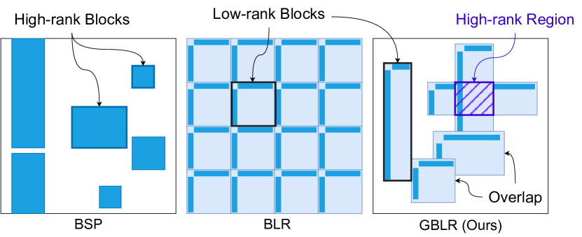
Figure 1: Comparison of block-sparse, block-low-rank, and our proposed Generalized block-low-rank matrices.

2.1 Block-related Matrices.

A block ${\bm{B}}\in\mathbb{R}^{|R|\times|C|}$ of a matrix ${\bm{W}}\in\mathbb{R}^{n\times n}$ is a submatrix of ${\bm{W}}$ with consecutive cyclic row and column indices. For example, $R$ can be $\{n-2,n-1,0,1\}$ if $|R|=4$. Also, we say two blocks ${\bm{B}}_{1}$ and ${\bm{B}}_{2}$ overlap if they have shared elements of ${\bm{W}}$.

Two well-known block-structured matrices are a block sparse (BSP) matrix and a block-low-rank (BLR)(Amestoy et al., 2015) matrix. Informally speaking, a matrix is block-sparse when non-zero elements are gathered in blocks and such blocks are sparse in the matrix. A block-low-rank matrix is composed of non-overlapping equally-partitioned low-rank blocks. Figure 1 illustrates the BSP and BLR matrices as well as our proposed generalized block-low-rank matrix, which we introduce in Section 3.1. We present the formal definitions of the block-sparse and block-low-rank matrices in Appendix A.1.

2.2 Structured Matrix

We say a matrix ${\bm{W}}\in\mathbb{R}^{n\times n}$ is structured if, for any ${\bm{x}}\in\mathbb{R}^{n}$, the matrix-vector product (MVP) ${\bm{y}}={\bm{W}}{\bm{x}}$ requires significantly less number of multiplications than $n^{2}$. For instance, LR, BSP, and BLR matrices are structured because the number of multiplications for MVP is determined by their (low) rank or sparsity. Although a general sparse matrix reduces the complexity of MVP to be a sub-quadratic function of $n$, it is excluded in our discussion of structured matrices because processing moderately sparse matrices (10$\sim$50% density) in conventional hardware such as GPUs does not reduce the actual run-time due to its unstructured positions of non-zero elements (Chen et al., 2022).

3 Proposed Method

We are interested in training a deep neural network (DNN) $f$ under a computational cost constraint:

$$\min_{f}\sum_{{\bm{x}},{\bm{y}}\sim{\mathcal{D}}}\mathcal{L}(f({\bm{x}}),{\bm{y}})\quad\text{s.t.}\quad\mathrm{cost}(f)\leq B,$$ (1)

where the first term is the cross-entropy loss for a classification task at a data point ${\bm{x}}$ and a label ${\bm{y}}$, and the constraint $\mathrm{cost}(f)$ is the number of multiplications to compute the neural network output $f({\bm{x}})$. Our method learns weight matrices of DNNs in a generalized structured matrix format in a differentiable, end-to-end manner.

3.1 Generalized Block-Low-Rank (GBLR) Matrix

We introduce a concept of a generalized structured matrix format that explains multiple popular structure matrices used in DNN training. The idea is that a block in a matrix can be expressed by a sum of rank-1 blocks, i.e., a rank-$r$ block is a sum of $r$ rank-1 blocks at the same position. In this manner, LR, BSP, and BLR matrices can be expressed under a unified framework (Theorem 1).

To be specific, our proposed structured matrix format is a generalized version of Block-Low-Rank (BLR) matrices. An $n$-by-$n$ Generalized Block-Low-Rank (GBLR) matrix ${\bm{W}}$ is obtained by overlapping multiple rank-1 blocks of different sizes at arbitrary locations, as depicted in Figure 2 (Left). The locations of the blocks as well as their element values are learned simultaneously from training data without explicit size or location restrictions.

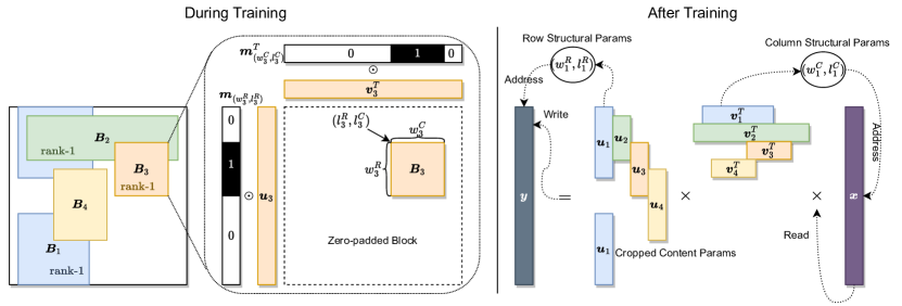
Figure 2: Left: An example of a GBLR matrix with 4 blocks. A block is generated from the structural parameters $(w^{R},l^{R}),(w^{C},l^{C})$ and the content parameters $({\bm{u}},{\bm{v}})$, where $(w^{R},l^{R})$ and $(w^{C},l^{C})$ form binary masks ${\bm{m}}_{(w^{R},l^{R})}$ and ${\bm{m}}_{(w^{C},l^{C})}$, respectively. Note that overlapped regions can have a rank higher than one. Right: Efficient Matrix-Vector Product computations using cropped content parameters and structural parameters. The structural parameters locate the input and output indices/addresses to read and write.

Suppose there are $K$ blocks: ${\bm{B}}_{1}\in\mathbb{R}^{w_{1}^{R}\times w_{1}^{C}},{\bm{B}}_{2}\in\mathbb{R}^{w_{2}^{R}\times w_{2}^{C}},\ldots,{\bm{B}}_{K}\in\mathbb{R}^{w_{K}^{R}\times w_{K}^{C}}$. Each block ${\bm{B}}_{k}$ has two parameter sets: 1) the structural parameters that identify the position of the block in the row and column index set ${\mathcal{I}}_{n-1}=\{0,1,\ldots,n-1\}$, and 2) the content parameters which specify the actual values of matrix elements.

Configuration of structural parameters. The position of a block is given by the indices of the rows and columns it occupies in the $n\times n$ matrix. Hence, the placement of a rectangle block can be identified by four numbers: width and location in terms of the row or column indices. Hence, we use a location parameter $l$ and a width parameter $w$ as the structural parameters of a block. Figure 2 (Left) illustrates a block of size $w^{R}\times w^{C}$ in an $n\times n$ matrix at location $(l^{R},l^{C})$. The row (column) index set of a block is the sequence of numbers from $l^{R}$ ($l^{C}$) to $l^{R}+w^{R}$ ($l^{C}+w^{C}$) where the addition is a cyclic/modulo addition. For each block ${\bm{B}}_{k}$ for $k=1,\ldots,K$, we have four parameters: $(w_{k}^{R},l_{k}^{R})$ for the row and $(w_{k}^{C},l_{k}^{C})$ for the column. We use the notation $\phi_{k}^{R}=(w_{k}^{R},l_{k}^{R})$ and $\phi_{k}^{C}=(w_{k}^{C},l_{k}^{C})$ to represent the tuple of width and location for the row ($\phi_{k}^{R}$) and column ($\phi_{k}^{C}$).

Based on the structural parameter $w_{k}^{C}$ and $l_{k}^{C}$, one can construct an $n$-dimensional binary mask that has $w_{k}^{C}\in{\mathcal{I}}_{n}$ consecutive ones starting from $l_{k}^{C}\in{\mathcal{I}}_{n-1}$ in the cyclic order:

$$m_{\phi_{k}^{C}}[j]=m_{(w_{k}^{C},l_{k}^{C})}[j]=\begin{cases}1&\text{if }l_{k}^{C}\leq j+an<l_{k}^{C}+w_{k}^{C}\\ 0&\text{otherwise}\end{cases},\>j\in{\mathcal{I}}_{n-1},\>a\in\{0,1\},$$ (2)

where $a\in\{0,1\}$ is necessary to make the order cyclic. We call the mask in Eq. 2 the boxcar mask since the non-zero elements are located consecutively. The boxcar mask is used to select $w_{k}^{C}$ (cyclic) consecutive non-zero elements of an $n$-dimensional vector. The mask for the rows ${\bm{m}}_{\phi_{k}^{R}}$ is obtained in the same way from $w_{k}^{R}$ and $l_{k}^{R}$.

Configuration of content parameters. To represent the values of a rank-1 block ${\bm{B}}_{k}$, we use two $n$-dimensional vectors ${\bm{u}}_{k}$ and ${\bm{v}}_{k}$ as content parameters along with the boxcar masks ${\bm{m}}_{\phi_{k}^{R}}$, ${\bm{m}}_{\phi_{k}^{C}}$. All these parameters $(\phi_{k}^{R},\phi_{k}^{C},{\bm{u}}_{k},{\bm{v}}_{k})$ are learned during the DNN training simultaneously. Since the boxcar masks ${\bm{m}}_{\phi_{k}^{R}}$ and ${\bm{m}}_{\phi_{k}^{C}}$ guide the location of the block in the $n\times n$ matrix, ${\bm{u}}_{k}$ and ${\bm{v}}_{k}$ are element-wise multiplied with the boxcar masks:

$$\mathrm{ZeroPad}({\bm{B}}_{k})=({\bm{m}}_{\phi_{k}^{R}}\odot{\bm{u}}_{k})({\bm{m}}_{\phi_{k}^{C}}\odot{\bm{v}}_{k})^{T},$$

where the resulting $n\times n$ matrix is a zero-padded block. Ideally, we expect the mask to expand / shrink and shift to find the right subset of the elements of a content parameter, while the content parameter updates the value of the elements selected by the mask.

Now we formally define the Generalized Block-low-rank (GBLR) format, which is the sum of $K$ zero-padded blocks:

$${\bm{W}} =\sum_{k=1}^{K}({\bm{m}}_{\phi_{k}^{R}}{\bm{m}}_{\phi_{k}^{C}}^{T})\odot({\bm{u}}_{k}{\bm{v}}_{k}^{T})=\sum_{k=1}^{K}\left({\bm{m}}_{\phi_{k}^{R}}\odot{\bm{u}}_{k}\right)\left({\bm{m}}_{\phi_{k}^{C}}\odot{\bm{v}}_{k}\right)^{T}.$$ (3)

A GBLR matrix is associated with an average width $\bar{w}=\frac{1}{2K}\sum_{k=1}^{K}w_{k}^{R}+w_{k}^{C}$.

Definition 1.

Let $\mathsf{GBLR}(n,K,s)$ be the set of matrices obtained by Eq. 3 for the average width less than or equal to $s$, i.e., $\bar{w}=\frac{1}{2K}\sum_{k=1}^{K}w_{k}^{R}+w_{k}^{C}\leq s$. A matrix ${\bm{W}}$ is an $(n,K,s)$-GBLR if ${\bm{W}}\in\mathsf{GBLR}(n,K,s)$.

We use the notation $\bm{\phi}({\bm{W}}):=({\bm{w}}({\bm{W}}),{\bm{l}}({\bm{W}}))$ to indicate the collection of the structural parameters of ${\bm{W}}$, where ${\bm{w}}({\bm{W}})=\{w_{1}^{R},w_{1}^{C},w_{2}^{R},w_{2}^{C},\ldots,w_{K}^{R},w_{K}^{C}\}$ and ${\bm{l}}({\bm{W}})=\{l_{1}^{R},l_{1}^{C},l_{2}^{R},l_{2}^{C},\ldots,l_{K}^{R},l_{K}^{C}\}$. We simply use $\bm{\phi}:=\bm{\phi}({\bm{W}})$ if ${\bm{W}}$ is clearly inferred in the context.

Efficiency. Once the structural parameters are fixed, it is unwise to store and use two $n$-dimensional content parameters for each block ${\bm{B}}_{k}$ because only $w_{k}^{R}$ elements of ${\bm{u}}_{k}$ and $w_{k}^{C}$ elements of ${\bm{v}}_{k}$ are non-zero according to the boxcar masks in eq. 3. Hence, one can store and use the cropped content parameters ${\bm{u}}_{l^{R}:l^{R}+w^{R}}$ and ${\bm{v}}_{l^{C}:l^{C}+w^{C}}$ for MVP between an input ${\bm{x}}\in\mathbb{R}^{n}$ (which can be also cropped from $l^{C}$ to $l^{C}+w^{C}$) and a block ${\bm{B}}$, as described below and in Figure 2 (Right):

$$\mathrm{ZeroPad}({\bm{B}}){\bm{x}} =({\bm{m}}_{(w^{R},l^{R})}\odot{\bm{u}})({\bm{m}}_{(w^{C},l^{C})}\odot{\bm{v}})^{T}{\bm{x}}$$

$$=\mathrm{ZeroPad}\left({\bm{u}}_{l^{R}:l^{R}+w^{R}}({\bm{v}}_{l^{C}:l^{C}+w^{C}}^{T}{\bm{x}}_{l^{C}:l^{C}+w^{C}})\right),$$

which requires only $w^{R}+w^{C}$ multiplications. Hence, the number of multiplications (denoted by FLOPs) for multiplying ${\bm{W}}\in\mathsf{GBLR}(n,K,s)$ with ${\bm{x}}\in\mathbb{R}^{n}$ is bounded by $2Ks$:

$$\text{FLOPs}=\sum_{k=1}^{K}(w_{k}^{R}+w_{k}^{C})=2K\bar{w}\leq 2Ks.$$ (4)

Expressiveness. Low-rank (LR), block sparse (BSP), and block-low-rank (BLR) matrices are popular structured matrices in the DNN literature, and they are special cases of the GLBR matrix under mild conditions. Proofs and formal definitions of LR, BSP, and BLR matrices are in Appendix A.1

Theorem 1.

Let $n,K,s$ be positive integers satisfying $Ks\geq n$. Then any $n$-by-$n$ rank-$\frac{Ks}{n}$ matrices and $(n,\frac{K}{s},s)$-block-sparse matrices are $(n,K,s)$-GBLR. Also, any $(n,K,s,1)$-block-low-rank matrices are $(n,K,s)$-GBLR if $K=(n/s)^{2}$.

More importantly, a new structured matrix obtained by interpolating the structural parameters of two $(n,K,s)$-GBLR matrices is still $(n,K,s)$-GBLR, based on Theorem 2. Therefore, a new type of structured matrices can be derived from a set of GBLR matrices.

Theorem 2 (Closed under structural interpolation).

Given two $n\times n$ matrices ${\bm{W}},{\bm{Z}}\in\mathsf{GBLR}(n,K,s)$, and $\alpha\in[0,1]$, consider the following combination between the structural parameters:

$${\bm{w}}^{\prime}=\lfloor\alpha{\bm{w}}({\bm{W}})+(1-\alpha){\bm{w}}({\bm{Z}})\rfloor,\quad{\bm{l}}^{\prime}=\lfloor\alpha{\bm{l}}({\bm{W}})+(1-\alpha){\bm{l}}({\bm{Z}})\rfloor.$$

A matrix ${\bm{Y}}$ generated by Eq. 3 with the structural parameter $({\bm{w}}^{\prime},{\bm{l}}^{\prime})$ is a $(n,K,s)$-GBLR matrix, ${\bm{Y}}\in\mathsf{GBLR}(n,K,s)$.

Theorem 1 and Theorem 2 tell us that $(n,K,s)$-GBLR matrices cover a wide range of popular existing structured matrices and also undiscovered ones. In the following section, we introduce a differentiable tool to find/learn structured matrices in $\mathsf{GBLR}(n,K,s)$.

3.2 Gaussian-Dirichlet (Gaudi) Mask

The matrix structure in the GBLR format is determined by the width and location parameters. We aim to extract/learn these structural parameters from training data using stochastic gradient descent. In order to do so, the non-differentiability of the boxcar mask parameters needs to be handled.

To tackle this issue, we introduce a Dirichlet-kernel-based parameterization of the boxcar to explicitly parameterize the width $w$ and location $l$ in the expression. Consider a boxcar mask of length $n$, width $w$, and location $l$. Let $\hat{{\bm{m}}}_{(w,l)}$ be the discrete Fourier transform (DFT) of the mask ${\bm{m}}_{(w,l)}$. The frequency-domain representation of the boxcar mask is given by

$$\hat{m}_{(w,l)}[k] =e^{-2\pi\imath\frac{k}{n}l}\hat{m}_{(w,0)}[k]=e^{-2\pi\imath\frac{k}{n}l}\sum_{j=0}^{w-1}e^{-2\pi\imath j\frac{k}{n}}=e^{-2\pi\imath\frac{k}{n}l}w\frac{\mathrm{sinc}\left(w\frac{k}{n}\right)}{\mathrm{sinc}\left(\frac{k}{n}\right)}e^{\imath\pi k\left(\frac{1-w}{n}\right)}$$ (5)

$$=e^{-2\pi\imath\frac{k}{n}l}d_{w}[k],$$

where $d_{w}[k]:=w\frac{\mathrm{sinc}\left(w\frac{k}{n}\right)}{\mathrm{sinc}\left(\frac{k}{n}\right)}e^{\imath\pi k\left(\frac{1-w}{n}\right)}$ is the Dirichlet kernel of order $n$ (Bruckner et al., 1997) in the discrete domain ${\mathcal{I}}_{n-1}=\{0,1,\ldots,n-1\}$.

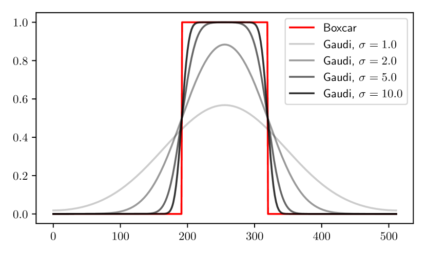
Figure 3: Comparison between Boxcar mask and Gaudi masks in the time domain with different smoothing factors $\sigma$. The Gaudi mask converges to the Boxcar mask as $\sigma$ grows.

Furthermore, we propose a smooth version of the Dirichlet-kernel-based mask by convolving the time-domain boxcar mask with the Gaussian-shape function. It is obtained in the frequency domain by element-wise multiplying the Gaussian function $g_{\sigma}[k]=\exp\left(-\frac{k^{2}}{2\sigma^{2}}\right)$ with the standard deviation $\sigma>0$ to the Dirichlet kernel. We call the resulting function the Gaussian-Dirichlet (Gaudi) function $\mathbf{d}_{w}^{\sigma}$:

$$\mathrm{d}_{w}^{\sigma}[k] :=g_{\sigma}(k)\cdot\mathrm{d}_{n}[k],$$

$$\tilde{\bm{m}}_{(w,l)}^{\sigma} :=\mathbf{IDFT}(\mathbf{d}_{w}^{\sigma}\cdot e^{-2\pi\imath\frac{{\bm{k}}}{n}l}),$$ (6)

where ${\bm{k}}=[0,1,\ldots,n-1]$. And we call the mask generated by a Gaudi function $\tilde{\bm{m}}_{(w,l)}^{\sigma}$ the Gaudi mask, where the parameter $\sigma$ controls the smoothness. Note that as $\sigma\to\infty$, the Gaudi mask converges to the boxcar mask (Lemma 5). Figure 3 visualizes the time-domain Gaudi mask approaching the boxcar mask.

A useful property of the Gaudi mask is that one can obtain exact derivatives with respect to the width parameter, even when the width is zero. To show it, we relax the domain of widths and locations to the continuous interval $[0,n]$ (see Appendix A.4).

Theorem 3.

Let $n<\infty$ be a finite positive integer. For any $\sigma\in(0,\infty]$ and $w,l\in[0,n]$, the derivatives of the Gaudi mask $\tilde{{\bm{m}}}_{(w,l)}^{\sigma}$ with respect to $w$ and $l$ are bounded almost everywhere:

$$\left\|\frac{\partial\tilde{{\bm{m}}}_{(w,l)}^{\sigma}}{\partial w}\right\|_{2}<\infty,\quad\left\|\frac{\partial\tilde{{\bm{m}}}_{(w,l)}^{\sigma}}{\partial l}\right\|_{2}<\infty.$$

Especially when $w=0$, the derivative with respect to $w$ is neither divergent nor zero.

Corollary 4.

For any $l\in[0,n]$ and $\sigma\in(0,\infty]$, the norm of the derivative of the Gaudi mask $\tilde{{\bm{m}}}_{(w,l)}^{\sigma}$ with respect to $w$ at $w=0$ is well-defined and greater than zero, i.e., $0<\left\|\frac{\partial\tilde{{\bm{m}}}_{(w,l)}^{\sigma}}{\partial w}\right\|_{2}<\infty$.

To allow learning the mask structural parameters in a differentiable manner, we plug the Gaudi mask (Eq. 6) into Eq. 3 as the mask of GBLR matrices to model Gaussian-Dirichlet GBLR (GauDi-GBLR) with parameters $\bm{\theta}=(\bm{\phi},{\bm{U}},{\bm{V}},\sigma)$:

$${\bm{W}}^{\bm{\theta}}={\bm{W}}^{(\bm{\phi},{\bm{U}},{\bm{V}},\sigma)}=\sum_{k=1}^{K}\left(\tilde{{\bm{m}}}_{\phi_{k}^{R}}^{\sigma}\odot{\bm{u}}_{k}\right)\left(\tilde{{\bm{m}}}_{\phi_{k}^{C}}^{\sigma}\odot{\bm{v}}_{k}\right)^{T}.$$ (7)

In practice, one can use small $\sigma\approx 1$ at the beginning of the training process to update the corresponding (unmasked) content parameters which are more than necessary, then gradually increase $\sigma$ to adjust the content parameters with a tighter mask. Since the purpose of using a Gaudi mask is to learn structural parameters of the GBLR matrix by Gradient Descent, Gaudi-GBLR matrices are later replaced by GBLR matrices once the structural parameters are found/learned. To compute MVP using GBLR matrices, one can use the cropped content parameters and inputs, as we discussed in Section 3.1-efficiency, without constructing masks at all. Hence, during the inference, there is no overhead to compute Gaudi masks.

Algorithm 1 GBLR Learning by PGD

1:repeat

2:     $({\bm{x}}_{1},{\bm{y}}_{1}),\ldots,({\bm{x}}_{M},{\bm{y}}_{M})\sim{\mathcal{D}}$

3:     $\ell\leftarrow\frac{1}{M}\sum_{i=1}^{M}{\mathcal{L}}(f^{\bm{\theta}}({\bm{x}}_{i}),{\bm{y}}_{i})$

4:     for trainable $p\in\bm{\theta}$ do

5:         $p\leftarrow p-\eta\cdot\mathrm{AdamW}(\nabla\ell)$

6:     end for

7:     for $k=1,2,\ldots,K$ do

8:         $w_{k}\leftarrow\mathrm{clip}(S_{\eta\lambda}(w_{k}),0,n)$

9:     end for

10:until converge

3.3 Learning Gaudi-GBLR for Efficient Neural Networks

We now introduce an algorithm to learn the structural parameters of Gaudi-GBLR matrices. The goal of the learning algorithm is to identify Gaudi-GBLR matrix structures (i.e., their parameters) that allow computationally efficient DNNs. Our discussion is centered around a two-layered multi-layer perception (MLP) for ease of understanding. However, the technique can be applied to general DNNs that incorporate linear layers.

Now let us consider a two-layered MLP $f^{\bm{\theta}}$ with a Gaudi-GBLR weight matrix ${\bm{W}}^{\bm{\theta}}$: $f^{\bm{\theta}}({\bm{x}})={\bm{h}}^{T}a({\bm{W}}^{\bm{\theta}}{\bm{x}}+{\bm{b}})$. We initially relax the domain of $w\in{\mathcal{I}}_{n}$ and $l\in{\mathcal{I}}_{n-1}$ of the Gaudi mask to the real-valued space $w,l\in[0,n]$ as we discuss in Appendix A.4. Due to the property of Gaudi-GBLR matrices Eq. 4, the computational cost constraint on the DNN $f^{\bm{\theta}}$ in Problem (1) can be replaced by a constraint on the sum of the width parameters of ${\bm{W}}^{\bm{\theta}}$. Specifically, we find width parameters of ${\bm{W}}^{\bm{\theta}}$ satisfying $\|{\bm{w}}\|_{1}\leq B$ since $\sum_{k=1}^{K}w_{k}=\|{\bm{w}}\|_{1}$. To solve the problem with Gradient Descent, we relax this $\ell_{1}$-norm constrained problem to a unconstrained one using the method of Lagrange multiplier:

$$\min_{\bm{\theta}}\sum_{({\bm{x}},{\bm{y}})\sim{\mathcal{D}}}{\mathcal{L}}(f^{\bm{\theta}}({\bm{x}}),{\bm{y}})+\lambda\|{\bm{w}}\|_{1},\quad\lambda\geq 0.$$ (8)

The resulting computational budget is implicitly constrained by a hyperparameter $\lambda\geq 0$.

Theorem 3 guarantees the derivatives of the widths and locations of the Gaudi-GBLR matrix in $f^{\bm{\theta}}$ can be obtained with any positive smoothing parameter $\sigma>0$ so that we can safely learn the parameters in the continuous domain $[0,n]$. Specifically, we update the width parameter ${\bm{w}}$ in the $\ell_{1}$-norm term in Problem (8) by Proximal Gradient Descent (PGD):

$${\bm{w}}_{t+1} =S_{\eta\lambda}({\bm{w}}_{t}-\eta\nabla{\mathcal{L}}(f^{\bm{\theta}}({\bm{x}}),{\bm{y}})),$$ (9)

where $S_{\mu}(x)=\begin{cases}\mathrm{sign}(x)\cdot(|x|-\mu)&\text{if $x>\mu$}\\ 0&\text{otherwise}\end{cases}$ is the element-wise soft shrinkage function. In practice, the gradient is calculated with an adaptive optimizer such as Adam (Kingma & Ba, 2014) or AdamW (Loshchilov & Hutter, 2017). The overall process is summarized in Algorithm 1. Although Problem (8) is non-linear, our experimental results show that PGD can attain good local optima with an adaptive optimizer and the initialization method we propose in Appendix A.2. A practical learning method for the width and location parameters defined in the discrete spaces ${\mathcal{I}}_{n}$ and ${\mathcal{I}}_{n-1}$ is discussed in Appendix A.5.

4 Experiments

We evaluate our proposed method by replacing the weight matrices of Vision Transformers (ViT) (Dosovitskiy et al., 2020), and MLP-Mixer (Tolstikhin et al., 2021) with Gaudi-GBLR matrices. For the experiment, we set the number of blocks $K$ equal to the number of columns of the matrix $n$. We also evaluate alternative schemes for comparisons where the weights are replaced by popular hand-designed structured matrix formats such as Low-Rank (LR), Block-Sparse-plus-Low-Rank (BSP-LR), and Block-low-rank (BLR). For LR matrices, we use singular vector decomposition to find the best rank-$s$ approximation of the given matrix for the predefined rank of $s$. Pixelfly (Chen et al., 2022) and Monarch (Dao et al., 2022) are schemes that use BSP-LR and BLR matrices respectively. We set the structural parameters of these alternative schemes to exhibit similar computational costs for MVP compared to our proposed scheme. Note that the structural parameter sets for LR, BSP-LR, and BLR do not change across different layers in the neural network. We FLOPs to denote the number of multiplications, and use 8 NVIDIA A40 GPUs in our experiments. The detailed experimental settings are described in Appendix A.6.

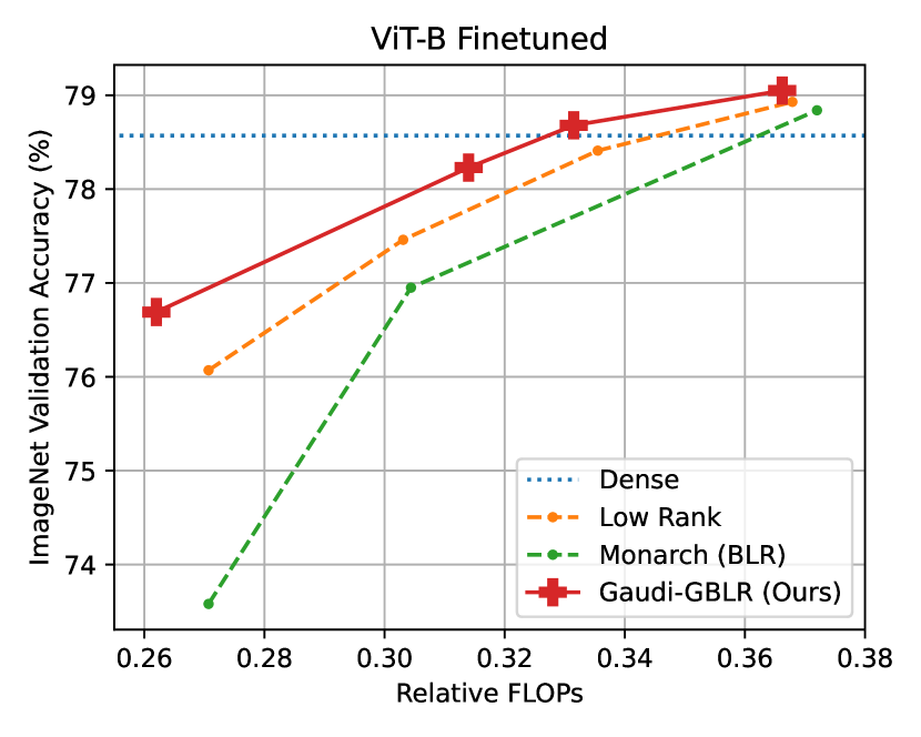
Figure 4: ImageNet accuracy after fine-tuning ViT-Base weights replaced with structured weight matrices. Dense: the original ViT-Base model.

4.1 Fine-tuning Results

We use the pre-trained weights of the ViT-Base on ImageNet and initialize the parameters of the Gaudi-GBLR matrices by Algorithm 2 in Section A.2. The ViTs with Gaudi-GBLR matrices were fine-tuned on ImageNet (Russakovsky et al., 2015). During the initialization, we set the computational budget of all matrices in the network the same. For a fair comparison, the same set of hyperparameters was used throughout our fine-tuning experiments.

The highest accuracy is achieved by Gaudi-GBLR in ViT-Base with a patch size of $16\times 16$ on the ImageNet validation dataset after fine-tuning it for 35 epochs. Figure 4 shows that Gaudi-GBLR preserves the accuracy well when the complexity is reduced to 30% of the original ‘Dense’ model which does not use structured matrices (its FLOPs count is normalized to 1). The other hand-designed approaches exhibit more significant accuracy degradations for the same complexity reduction. Overall, Gaudi-GBLR strikes better Accuracy-FLOPs trade-offs than LR or Monarch approaches. The higher accuracy for a similar FLOPs count quantifies the gain from the learned structured matrices.

4.2 Training From Scratch

We train ViTs (Dosovitskiy et al., 2020) and MLP-Mixers (Tolstikhin et al., 2021) with structured weight matrices on CIFAR-10&100 (Krizhevsky et al., 2009) by Algorithm 1 from randomly-initialized content parameters. We set $\sigma=1$ for the first epoch and gradually increase it to $100$ until the training process ends. In Figure 5, we study the accuracy-FLOPs trade-off using CIFAR10/100 datasets when the models are trained from scratch (i.e., not fine-tuned from pre-trained weights). As in the ImageNet fine-tuning experiment, Gaudi-GBLR achieves superior accuracy-FLOPs trade-offs outperforming the other hand-designed structured matrices.

Table 1: ImageNet accuracies and GFLOPs on a $224\times 224$ image of ViT-Base models trained from scratch with dense matrices and Gaudi-GBLR matrices.

Model	Acc. (%)	GFLOPs
ViT-Base	78.57	17.2
w/ Gaudi-GBLR	78.51	5.65

Table 2: FLOPs by type of linear layers with Gaudi-GBLR matrix of ViT-Base trained on ImageNet. Units in KFLOPs ($10^{3}$ FLOPs).

Layer Type	Min	Max	Avg
Query	4.2	67.6	29.0
Key	11.6	87.6	42.1
Value	34.2	135.5	95.0
MLP-FC1	359.8	910.2	597.7
MLP-FC2	349.4	1,175.2	756.6

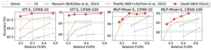
Figure 5: Accuracy-Cost trade-off of models trained from scratch on CIFAR-10/100 dataset.

4.3 Analysis on Learned Gaudi-GBLR Matrices

In this section, we study the learned Gaudi-GBLR matrices in terms of computational budget allocation, and mask patterns. The analysis is based on ViT-Base Gaudi-GBLR matrices trained on ImageNet from scratch by following the same $\sigma$ adaptation rule used in CIFAR10/100 experiments. The accuracy and FLOPs of the ViT-Base with Gaudi-GBLR is reported in Table 1.

Learned Computational Budget Allocation.

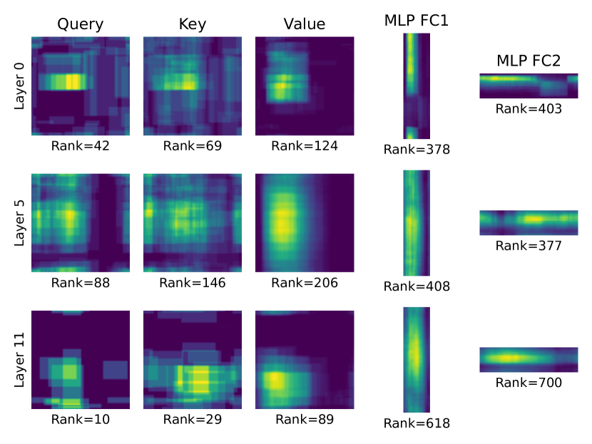
Figure 6: Mask patterns of weights for Query, Key, Value, FC1 and FC2 in Layer 0, 5, and 11 (out of $0\sim 11$). The brighter, the more overlapped blocks. The numbers below indicate the rank of the matrix (max: 768).

The proposed learning framework automatically allocates the computational budget to all linear layers of ViT-Base during the training process given by Algorithm 1. The algorithm finds a well-balanced (not necessarily equal) allocation for each matrix to meet the overall cost budget while minimizing the loss function. As a result, Gaudi-GBLR weight matrices in the network have unequal widths requiring different FLOPs for each MVP. Table 2 summarizes the min/max/average FLOPs statistics collected for different types of linear layers. Within an Attention layer, the weights for Values have the highest budget whereas Queries and Keys use a smaller budget. The smallest layer uses only about 4,200 FLOPs for MVP involving a $768\times 768$ matrix and a $768\times 1$ vector. The FLOPs assigned to the linear layer of channel MLPs (MLP-FC1 and MLP-FC2 in Table 2) vary significantly. Although the size of the weight matrix used in the MLPs are $4\times$ larger than the ones used for Value, the MLP-FC2-type layers use $7.96\times$ FLOPs than the Value-type layers in average.

Visualization. Figure 6 visualizes the locations of the blocks in exemplary Gaudi-GBLR weight matrices of ViT-Base trained from scratch. We select the first, middle, and the last layers of different types: linear layers for Query, Key, Values in Attention modules, and two linear layers (FC1 and FC2) in MLPs. Bright colors in Figure 6 highlight regions where masks are overlapped. The rank of each weight matrix is marked under each visualized mask pattern. Interestingly, the resulting matrix is neither BSP nor BLR. It is observed that blocks are concentrated in a small number of regions. We believe this is related to the Multi-Head (Vaswani et al., 2017) scheme of the ViT. Each weight matrix of an attention layer is a collection of weights for multiple heads. It is expected that some heads have more significant impacts on the output while others may not contribute as much. Hence multiple blocks are allocated to regions that correspond to those heads. Notice the rank of matrices obtained from the GBLR framework differs significantly across different layers and matrix types (Values, Queries, and Keys).

5 Related Works

Structured Matrices for DNNs. Prior works have identified that the weights have simple structures under certain conditions (Yaras et al., 2023; Huh et al., 2021; Gunasekar et al., 2017). However, explaining the structure of every weight matrix in practical DNNs such as Transformers (Vaswani et al., 2017) is still a challenging problem. Hence, prior works have focused on manually designing suitably structured matrices for DNNs. Hsu et al. (2022) used weighted low-rank decomposition for the weights of language models. Butterfly matrices (Li et al., 2015; Dao et al., 2019), inspired by Fast Fourier Transform (FFT), were adopted in the form of Block-Sparse (BSP) format (Pixelfly) by Chen et al. (2022), and also in the form of Block-low-rank (BLR) format (Monarch) by Dao et al. (2022). Unlike these prior works that rely on manual designs, our method learns the structure of weight matrices from the training data by stochastic gradient descent.

Mask Learning Masking is a popular technique to prune neurons or activations of the DNNs. Since a mask for neuron pruning/selection is a non-differentiable binary vector, its gradient does not exist almost everywhere. Jang et al. (2016) and Maddison et al. (2016) propose alternative distributions close to the Bernoulli distribution, which allow the continuous gradient. Movement Pruning in (Sanh et al., 2020) utilizes Straight-Through Estimator (STE) (Hinton, 2012; Bengio et al., 2013; Zhou et al., 2016) to pass the gradient through the Top-$k$ function. Lin et al. (2017) adopts deep reinforcement learning to select the input-dependent mask. On the contrary, our mask design solves the non-existing gradient problem by Gaudi-function-based parameterization in the frequency domain without using a surrogate or approximated gradient.

One-shot Neural Architecture Search. Neural Architecture Search (NAS) (Zoph & Le, 2016; Liu et al., 2018) seeks the optimal neural network structures from training data. To improve search efficiency, Pham et al. (2018); Liu et al. (2018) adopt the one-shot NAS technique that selects sub-network candidates from a super-network. Our method also falls into a similar category of finding a small-sized neural network in the scope of a structured matrix format while gradually converging to a smaller structure from a super-network given by the baseline network.

Frequency-domain Learning DiffStride (Riad et al., 2022) learns a stride of the pooling operation for images by cropping a rectangular region of the frequency response of an image. Riad et al. (2022) utilizes an approximated boxcar mask for a differentiable function. Although DiffStride shares similar components with Gaudi masks, the fundamental difference is in the design of the mask. We parameterize the mask in the frequency domain where widths and locations inherit the exact gradient.

6 Conclusion

We propose a generalized and differentiable framework for learning structured matrice for efficient neural networks by gradient descent. We introduce a new generalized format of structured matrices and parameterize the structure in the frequency domain by the Gaussian-Dirichlet (Gaudi) function with a well-defined gradient. Effective learning algorithms are provided for our framework showing flexibility and differentiability to find expressive and efficient structures from training data in an end-to-end manner. Evaluation results show that the proposed framework provides the most efficient and accurate neural network models compared to other hand-designed popular structured matrices.

7 Reproducibility Statement

The authors make the following efforts for reproducibility: 1) We attach the complete source code used in our experiment as supplemental materials, 2) we provide the detailed settings and hyperparameters in Section 4, A.5, and A.6, and 3) the proofs of all theorems, lemmas, and corollaries are presented in Section A.1.

Appendix A Appendix

A.1 Proofs

In this section, we provide the missing definitions, propositions, and proofs. The original theorems are restated for completeness.

A.1.1 Definitions

We introduce formal definitions of the block-related matrices discussed in our paper.

Definition 2 (Block-sparse matrix).

An $n$-by-$n$ matrix is $(n,m,s)$-block-sparse (BSP) if it contains $m$ non-overlapping non-zero blocks whose dimension is at most $s\times s$.

A $(n,m,s)$-block-sparse matrix may contain blocks of different sizes, but each of them has maximum $s\times s$ elements.

Definition 3 (Block-low-rank matrix (Amestoy et al., 2015; Jeannerod et al., 2019)).

An $n$-by-$n$ matrix is $(n,m,s,r)$-block-low-rank (BLR) if, when it is equally partitioned into $m=p\times p$ non-overlapping blocks of dimension $s\times s$, every block has a rank at most $r\ll\frac{n}{p}$.

The $(n,m,s,r)$-BLR matrix has blocks of the same size that tile the entire matrix.

A.1.2 Proof of Theorem 1

Theorem 1.

Let $n,K,s$ be positive integers satisfying $Ks\geq n$. Then any $n$-by-$n$ rank-$\frac{Ks}{n}$ matrices and $(n,\frac{K}{s},s)$-block-sparse matrices are $(n,K,s)$-GBLR. Also, any $(n,K,s,1)$-block-low-rank matrices are $(n,K,s)$-GBLR if $K=(n/s)^{2}$.

Proof.

It is sufficient to find the structural parameters of an $(n,K,s)$-GBLR matrix for each structured matrix format. Let ${\bm{w}}^{R},{\bm{w}}^{C}\in{\mathcal{I}}_{n}^{K}$ be the width parameters of rows and columns of the $(n,K,s)$-GBLR matrix, respectively, and ${\bm{l}}^{R},{\bm{l}}^{C}\in{\mathcal{I}}_{n-1}^{K}$ be the locations parameters of rows and columns, respectively, where ${\mathcal{I}}_{n}=\{0,1,\ldots,n\}$.

Low Rank Matrix. The rank-$\frac{Ks}{n}$ matrix is equivalent to the GBLR matrix with $Ks/n$ full-sized rank-1 blocks, i.e., ${\bm{w}}^{R}={\bm{w}}^{C}=[\underbrace{n,n,\ldots,n}_{Ks/n},0,0,\ldots,0]$ and ${\bm{l}}^{R}={\bm{l}}^{C}=\bm{0}$.

Block Sparse Matrix. A block of the $(n,\frac{K}{s},s)$-block-sparse matrix can have full rank. Consider a rank-1 block ${\bm{B}}$ of a $(n,K,s)$-GBLR matrix with some location parameters where the sum of the row width and the column width is $2s$. The maximum dimension of the block ${\bm{B}}$ is $s\times s$. Then clone and overlap the identical block with the same location and width parameters $s$ times to form a full-rank block of the dimension at most $s\times s$. Since the full-rank block can be generated $K/s$ times, any $(n,K/s,s)$-block-sparse matrix can be modeled by the corresponding width parameters and the location parameters.

Block Low rank Matrix. Since $K=\frac{n^{2}}{s^{2}}$, let us divide the $n$-by-$n$ matrix into $(n/s)^{2}$ blocks of the dimension of $s$-by-$s$. Assign the width and the location parameters correspondingly. The resulting matrix forms the $(n,K,s,1)$-block-low-rank matrix. ∎

A.1.3 Proof of Theorem 2

Theorem 2 (Closed under structural interpolation).

Given two $n\times n$ matrices ${\bm{W}},{\bm{Z}}\in\mathsf{GBLR}(n,K,s)$, and $\alpha\in[0,1]$, consider the following combination between the structural parameters:

$${\bm{w}}^{\prime}=\lfloor\alpha{\bm{w}}({\bm{W}})+(1-\alpha){\bm{w}}({\bm{Z}})\rfloor,\quad{\bm{l}}^{\prime}=\lfloor\alpha{\bm{l}}({\bm{W}})+(1-\alpha){\bm{l}}({\bm{Z}})\rfloor.$$

A matrix ${\bm{Y}}$ generated by Eq. 3 with the structural parameter $({\bm{w}}^{\prime},{\bm{l}}^{\prime})$ is a $(n,K,s)$-GBLR matrix, ${\bm{Y}}\in\mathsf{GBLR}(n,K,s)$.

Proof.

Let ${w^{\prime}}_{k}^{R}$ and ${w^{\prime}}_{k}^{C}$ be the width of the row and the column of the $k$th block of ${\bm{Y}}$, respectively. We use the same style of notation for $w({\bm{W}})_{k}^{R},w({\bm{W}})_{k}^{C}$ and $w({\bm{Z}})_{k}^{R},w({\bm{Z}})_{k}^{C}$ to denote the row and column width of the $k$th block of ${\bm{W}}$ and ${\bm{Z}}$. The interpolated matrix ${\bm{Y}}$ is $(n,K,s)$-GBLR if and only if the mean of the elements of ${\bm{w}}^{\prime}$ is less than or equal to $s$, or equivalently the sum of the elements is less than or equal to $2Ks$. Also, both ${\bm{W}}$ and ${\bm{Z}}$ have $2Ks$ sum of the width parameters. From this, the sum of the interpolated width is less than or equal to $2Ks$:

$$\sum_{i}{\bm{w}}^{\prime}_{i} =\sum_{k=1}^{K}{w^{\prime}}_{k}^{R}+{w^{\prime}}_{k}^{C}$$

$$=\sum_{k=1}^{K}\lfloor\alpha w({\bm{W}})_{k}^{R}+(1-\alpha)w({\bm{Z}})_{k}^{R}\rfloor+\lfloor\alpha w({\bm{W}})_{k}^{C}+(1-\alpha)w({\bm{Z}})_{k}^{C}\rfloor$$

$$\leq\sum_{k=1}^{K}\alpha w({\bm{W}})_{k}^{R}+(1-\alpha)w({\bm{Z}})_{k}^{R}+\alpha w({\bm{W}})_{k}^{C}+(1-\alpha)w({\bm{Z}})_{k}^{C}$$

$$=\alpha\sum_{k=1}^{K}(w({\bm{W}})_{k}^{R}+w({\bm{W}})_{k}^{C})+(1-\alpha)\sum_{k=1}^{K}(w({\bm{W}})_{k}^{R}+w({\bm{W}})_{k}^{C})$$

$$\leq\alpha 2Ks+(1-\alpha)2Ks$$

$$=2Ks.$$

Hence the interpolated matrix ${\bm{Y}}\in\mathsf{GBLR}(n,K,s)$. ∎

A.1.4 Proof of Lemma 5

Lemma 5.

Let $n\in{\mathbb{N}}$ be a positive integer. Let $l\in{\mathcal{I}}_{n-1}$ and $w\in{\mathcal{I}}_{n}$. Consider the discrete boxcar mask ${\bm{m}}_{(w,l)}$ with the structural parameter $(w,l)$ as in Eq. 2 and the Gaudi mask $\tilde{{\bm{m}}}_{(w,l)}^{\sigma}$ with the same parameters and $\sigma>0$ as in Eq. 6. Then $\tilde{{\bm{m}}}_{(w,l)}^{\sigma}$ converges to ${\bm{m}}_{(w,l)}$ as $\sigma\to\infty$, where the bound between two at $\sigma$ is given as follows:

$$\frac{\|{\bm{m}}_{(w,l)}-\tilde{\bm{m}}_{(w,l)}^{\sigma}\|_{2}}{\|{\bm{m}}_{(w,l)}\|_{2}}\leq 1-e^{-\frac{(1-n^{-1})^{2}}{2\sigma^{2}}}.$$

Proof.

By Parseval’s theorem,

$$\|{\bm{m}}_{(w,l)}-\tilde{{\bm{m}}}_{(w,l)}^{\sigma}\|_{2}^{2} =\frac{1}{n}\|\hat{{\bm{m}}}_{(w,l)}-\hat{\tilde{{\bm{m}}}}_{(w,l)}^{\sigma}\|_{2}^{2}$$ (10)

$$=\frac{1}{n}\sum_{k=0}^{n-1}\left|\mathrm{d}_{w}[k]-\mathrm{d}_{w}[k]e^{-\frac{k^{2}}{2\sigma^{2}}}\right|^{2}$$

$$=\frac{1}{n}\sum_{k=0}^{n-1}\left|\mathrm{d}_{w}[k]\right|^{2}\left(1-e^{-\frac{k^{2}}{2\sigma^{2}}}\right)^{2}$$

$$\leq\frac{1}{n}\sum_{k=0}^{n-1}\left|\mathrm{d}_{w}[k]\right|^{2}\left(1-e^{-\frac{\left(\frac{n-1}{n}\right)^{2}}{2\sigma^{2}}}\right)^{2}$$

$$=\|{\bm{m}}_{(w,l)}\|_{2}^{2}\left(1-e^{-\frac{\left(1-\frac{1}{n}\right)^{2}}{2\sigma^{2}}}\right)^{2},$$ (11)

where Eq. 11 is also due to Parseval’s theorem.

∎

A.1.5 Proof of Theorem 3

Let us first consider the derivative of the sinc function in eq. 5.

Lemma 6.

$\frac{\mathrm{d}\mathrm{sinc}\frac{wk}{n}}{\mathrm{d}w}=\frac{\cos\frac{\pi wk}{n}}{w}-\frac{\mathrm{sinc}\frac{wk}{n}}{w}$.

Proof.

$$\frac{\mathrm{d}\mathrm{sinc}\frac{wk}{n}}{\mathrm{d}w} =\frac{\mathrm{d}}{\mathrm{d}w}\frac{\sin\frac{\pi wk}{n}}{\frac{\pi wk}{n}}$$

$$=-\left(\frac{\pi wk}{n}\right)^{-2}\frac{\pi k}{n}\sin\frac{\pi wk}{n}+\left(\frac{\pi wk}{n}\right)^{-1}\cos\frac{\pi wk}{n}\cdot\frac{\pi k}{n}$$

$$=\frac{\cos\frac{\pi wk}{n}}{w}-\frac{\sin\frac{\pi wk}{n}}{\left(\frac{\pi wk}{n}\right)^{2}}$$

$$=\frac{\cos\frac{\pi wk}{n}}{w}-\frac{\mathrm{sinc}\frac{wk}{n}}{w}.$$

∎

The following lemma is useful for proving Theorem 3.

Lemma 7.

For any $\sigma\in(0,\infty]$ and $w,l\in[0,n]$, the derivative of the Gaudi function ${\bm{d}}_{(w,l)}^{\sigma}$ with respect to $w$ is as follows:

$$\frac{\partial{d}_{w}^{\sigma}[k]}{\partial w} =e^{-2\pi\imath\frac{k}{n}w}\cdot e^{\pi\imath\frac{k}{n}}\cdot e^{-\frac{k^{2}}{2\sigma^{2}}}\cdot\frac{1}{\mathrm{sinc}\frac{k}{n}}.$$

Proof.

Let us merge the terms of the Gaudi function $\mathrm{d}_{w}^{\sigma}[k]$ that does not contain $w$ into $C_{k}$:

$$\mathrm{d}_{w}^{\sigma}[k] =e^{-\frac{k^{2}}{2\sigma^{2}}}\cdot w\cdot\frac{\mathrm{sinc}\frac{wk}{n}}{\mathrm{sinc}\frac{k}{n}}e^{\frac{\imath\pi k(1-w)}{n}}$$

$$=w\cdot\mathrm{sinc}\frac{wk}{n}\cdot e^{\frac{-\imath\pi kw}{n}}\cdot C_{k}$$

where $C_{k}=e^{\pi\imath\frac{k}{n}}e^{-\frac{k^{2}}{2\sigma^{2}}}\frac{1}{\mathrm{sinc}\frac{k}{n}}$. From Lemma 6, the derivative of the Gaudi function with respect to $w$ is as follows:

$$\frac{\partial}{\partial w}\mathrm{d}_{w}^{\sigma}[k] =C_{k}\cdot\frac{\partial}{\partial w}\left(w\cdot\mathrm{sinc}\frac{wk}{n}\cdot e^{\frac{-\imath\pi kw}{n}}\right)$$

$$=C_{k}\cdot\left(\mathrm{sinc}\frac{wk}{n}e^{-\pi\imath\frac{k}{n}w}+\left(\frac{\cos\frac{\pi wk}{n}-\mathrm{sinc}\frac{wk}{n}}{w}\right)we^{-\pi\imath\frac{k}{n}w}+w\mathrm{sinc}\frac{wk}{n}\cdot\left(-\pi\imath\frac{k}{n}\right)e^{-\pi\imath\frac{k}{n}w}\right)$$

$$=C_{k}\cdot(\cos\frac{\pi wk}{n}-\imath\sin\frac{\pi wk}{n})$$

$$=C_{k}\cdot e^{-\imath\pi\frac{k}{n}w}.$$

∎

Now we prove Theorem 3.

Theorem 3.

Let $n<\infty$ be a finite positive integer. For any $\sigma\in(0,\infty]$ and $w,l\in[0,n]$, the derivatives of the Gaudi mask $\tilde{{\bm{m}}}_{(w,l)}^{\sigma}$ with respect to $w$ and $l$ are bounded almost everywhere:

$$\left\|\frac{\partial\tilde{{\bm{m}}}_{(w,l)}^{\sigma}}{\partial w}\right\|_{2}<\infty,\quad\left\|\frac{\partial\tilde{{\bm{m}}}_{(w,l)}^{\sigma}}{\partial l}\right\|_{2}<\infty.$$

Proof.

Here we use Parseval’s theorem again:

$$\left\|\frac{\partial\tilde{{\bm{m}}}_{(w,l)}^{\sigma}}{\partial w}\right\|_{2}^{2} =\frac{1}{n}\sum_{k=0}^{n-1}\left|\frac{\partial}{\partial w}\mathrm{d}_{w}^{\sigma}[k]e^{-2\pi\imath\frac{k}{n}l}\right|\left|\frac{\partial}{\partial w}\mathrm{d}_{w}^{\sigma}[k]e^{-2\pi\imath\frac{k}{n}l}\right|^{*}$$

$$=\frac{1}{n}\sum_{k=0}^{n-1}\left|e^{-2\pi\imath\frac{k}{n}w}\cdot e^{\pi\imath\frac{k}{n}}\cdot e^{-\frac{k^{2}}{2\sigma^{2}}}\cdot\frac{1}{\mathrm{sinc}\frac{k}{n}}e^{-2\pi\imath\frac{k}{n}l}\right|^{2}$$

$$=\frac{1}{n}\sum_{k=0}^{n-1}\left|e^{-\frac{k^{2}}{2\sigma^{2}}}\cdot\frac{1}{\mathrm{sinc}\frac{k}{n}}\right|^{2}$$

$$\leq\frac{1}{n}\sum_{k=0}^{n-1}\left|\frac{1}{\mathrm{sinc}\frac{n-1}{n}}\right|^{2}$$

$$<\infty,$$

where the first inequality used the fact that $e^{-\frac{k^{2}}{2\sigma^{2}}}\leq 1$ and $\frac{1}{\mathrm{sinc}\frac{k}{n}}\leq\frac{1}{\mathrm{sinc}\frac{n-1}{n}}$ for $k=0,1,\ldots,n-1$. Similarly, the bound on the norm of the derivative with respect to the location parameter can be also derived as below:

$$\left\|\frac{\partial\tilde{{\bm{m}}}_{(w,l)}^{\sigma}}{\partial l}\right\|_{2}^{2} =\frac{1}{n}\sum_{k=0}^{n-1}\left|\mathrm{d}_{w}^{\sigma}[k]\frac{\partial}{\partial l}e^{-2\pi\imath\frac{k}{n}l}\right|\left|\mathrm{d}_{w}^{\sigma}[k]\frac{\partial}{\partial l}e^{-2\pi\imath\frac{k}{n}l}\right|^{*}$$

$$=\frac{1}{n}\sum_{k=0}^{n-1}\left|\frac{\mathrm{sinc}\frac{wk}{n}}{\mathrm{sinc}\frac{k}{n}}e^{-\frac{k^{2}}{2\sigma^{2}}}e^{-\frac{2\pi\imath(1-w)}{n}}(-2\pi\imath\frac{k}{n})e^{-2\pi\imath\frac{k}{n}l}\right|^{2}$$

$$\leq\frac{1}{n}\sum_{k=0}^{n-1}\left|\frac{1}{\mathrm{sinc}\frac{n-1}{n}}2\pi\frac{n-1}{n}\right|^{2}$$

$$<\infty.$$

∎

A.1.6 Proof of Corollary 4

Before proving Corollary 4, we introduce another Corollary of Lemma 7.

Corollary 8.

For any $\sigma\in(0,\infty]$ and $w,l\in[0,n]$, the derivatives of the Gaudi mask $\tilde{{\bm{m}}}_{(w,l)}^{\sigma}$ with respect to $w$ and $l$ are given as follows:

$$\frac{\partial\tilde{m}_{(w,l)}^{\sigma}[k]}{\partial w} =\frac{1}{n}\sum_{k=0}^{n-1}F_{jk}^{*}\cdot e^{-2\pi\imath\frac{k}{n}(w+l)}\cdot e^{\pi\imath\frac{k}{n}}\cdot e^{-\frac{k^{2}}{2\sigma^{2}}}\cdot\frac{1}{\mathrm{sinc}\frac{k}{n}},$$

$$\frac{\partial\tilde{m}_{(w,l)}^{\sigma}[k]}{\partial l} =\frac{1}{n}\sum_{k=0}^{n-1}F_{jk}^{*}\cdot\left(-2\pi\imath\frac{k}{n}\right)\cdot e^{-2\pi\imath\frac{k}{n}l}\cdot\mathrm{d}_{w}^{\sigma}[k],$$

where $F_{jk}^{*}=e^{2\pi\imath j\frac{k}{n}}$ is the $(j,k)$th element of the inverse discrete Fourier transform (IDFT) matrix.

Proof.

By linearity of differentiation and Lemma 7

$$\frac{\partial}{\partial w}\tilde{m}_{(w,l)}^{\sigma}[k] =\frac{\partial}{\partial w}\frac{1}{n}\sum_{k=0}^{n-1}F_{jk}^{*}\cdot e^{-2\pi\imath\frac{k}{n}l}\cdot\mathrm{d}_{w}^{\sigma}[k]$$

$$=\frac{1}{n}\sum_{k=0}^{n-1}F_{jk}^{*}\cdot e^{-2\pi\imath\frac{k}{n}l}\cdot\frac{\partial}{\partial w}\mathrm{d}_{w}^{\sigma}[k]$$

$$=\frac{1}{n}\sum_{k=0}^{n-1}F_{jk}^{*}\cdot e^{-2\pi\imath\frac{k}{n}l}\cdot e^{-2\pi\imath\frac{k}{n}w}\cdot e^{\pi\imath\frac{k}{n}}\cdot e^{-\frac{k^{2}}{2\sigma^{2}}}\cdot\frac{1}{\mathrm{sinc}\frac{k}{n}}$$

$$=\frac{1}{n}\sum_{k=0}^{n-1}F_{jk}^{*}\cdot e^{-2\pi\imath\frac{k}{n}(w+l)}\cdot e^{\pi\imath\frac{k}{n}}\cdot e^{-\frac{k^{2}}{2\sigma^{2}}}\cdot\frac{1}{\mathrm{sinc}\frac{k}{n}}.$$

The derivative with respect to the location parameter is a direct consequence of the derivative of the exponential function. ∎

Corollary 4.

For any $l\in[0,n]$ and $\sigma\in(0,\infty]$, the norm of the derivative of the Gaudi mask $\tilde{{\bm{m}}}_{(w,l)}^{\sigma}$ with respect to $w$ at $w=0$ is well-defined and greater than zero, i.e., $0<\left\|\frac{\partial\tilde{{\bm{m}}}_{(w,l)}^{\sigma}}{\partial w}\right\|_{2}<\infty$.

Proof.

From Corollary 8

$$\left.\frac{\partial\tilde{m}_{(w,l)}^{\sigma}[k]}{\partial w}\right|_{w=0} =\frac{1}{n}\sum_{k=0}^{n-1}F_{jk}^{*}\cdot e^{-2\pi\imath\frac{k}{n}l}\cdot e^{\pi\imath\frac{k}{n}}\cdot e^{-\frac{k^{2}}{2\sigma^{2}}}\cdot\frac{1}{\mathrm{sinc}\frac{k}{n}}.$$

Since $e^{-2\pi\imath\frac{k}{n}l}\cdot e^{\pi\imath\frac{k}{n}}\cdot e^{-\frac{k^{2}}{2\sigma^{2}}}\cdot\frac{1}{\mathrm{sinc}\frac{k}{n}}$ is not zero for any $l\in[0,n]$ and $\sigma\in(0,\infty]$ and the IDFT matrix ${\bm{F}}^{*}$ is unitary (up to scaling factor), the derivative $\frac{\partial}{\partial w}\tilde{{\bm{m}}}_{(w,l)}^{\sigma}\neq\bm{0}$. ∎

A.2 Initialization Algorithm

Suppose an $n$-by-$n$ matrix ${\bm{W}}_{\text{init}}$ is given before the initialization step. We first initialize the structural parameters based on the correlation within the columns of ${\bm{W}}_{\text{init}}$.

Consider the Gram matrix ${\bm{C}}={\bm{W}}_{\text{init}}^{T}{\bm{W}}_{\text{init}}$. $C_{ij}={\bm{W}}_{:,i}^{T}{\bm{W}}_{:,j}$ is the inner product between the $i$th column and the $j$th column of ${\bm{W}}_{\text{init}}$. That is, the higher $|C_{ij}|$ is, the more correlated the columns are. Thus, for the width and the location parameter of the column of the first block, we pick a row of the Gram matrix ${\bm{C}}_{i_{1},:}$ where $i_{1}$ is the index of the row which has the largest norm. Then we apply a smoothing filter (e.g., Gaussian filter with the standard deviation $\gamma>0$) to the absolute values of the row, which is followed by binarizing the filtered output based on some threshold $\tau>0$. Hence, for the $k$th block, it can be summarized as follows:

$$b_{i_{k}}[j] =\begin{cases}1&c_{i_{k}}[j]\geq\tau\\ 0&c_{i_{k}}[j]<\tau\end{cases},\quad{\bm{c}}_{i_{k}}=\mathrm{Filter}(|{\bm{C}}_{i_{k},:}|,\gamma),\quad i_{k}=\mathrm{argsort}(\{\|{\bm{C}}_{i,:}\|_{2}\}_{i=1}^{n})[k].$$ (12)

As a result, the binary vector ${\bm{b}}_{i}$ consists of the chunks of ones and zeros. We choose the longest chunk of ones and initialize the width and the location parameters $(w_{k}^{C},l_{k}^{C})$ correspondingly. For the row parameters of the $k$th block, the same procedure is repeated with the columns of ${\bm{W}}_{\text{init}}$ selected in the column parameter initialization step.

Next, the content parameters are set by the left and the right singular vectors of ${\bm{W}}_{\text{init}}$ scaled by the singular values, i.e., ${\bm{U}}\leftarrow{\bm{U}}_{\text{init}}{\bm{S}}_{\text{init}}^{1/2}$ and ${\bm{V}}\leftarrow{\bm{S}}_{\text{init}}^{1/2}{\bm{V}}^{T}$ where ${\bm{W}}_{\text{init}}={\bm{U}}_{\text{init}}{\bm{S}}_{\text{init}}{\bm{V}}_{\text{init}}^{T}$.

Finally, we update the structural parameters and content parameters by minimizing the following objective function:

$$\min_{{\bm{U}},{\bm{V}},\bm{\phi}}\left\|{\bm{W}}_{\text{init}}-{\bm{W}}^{\bm{\theta}}\right\|_{F}^{2}+\lambda\|{\bm{w}}\|_{1}+\bm{1}_{{\bm{w}}\in{\mathcal{I}}_{n}^{n}}+\bm{1}_{{\bm{l}}\in{\mathcal{I}}_{n-1}^{n}}$$ (13)

We summarize the initialization steps in Algorithm 2.

Algorithm 2 GBLR Parameter Initialization

1:${\bm{C}}\leftarrow{\bm{W}}^{T}{\bm{W}}$ $\triangleright$ Target matrix ${\bm{W}}\in\mathbb{R}^{n\times n}$

2:$i_{1},i_{2},\ldots,i_{n}\leftarrow\mathrm{argsort}(\{\|{\bm{C}}_{i,:}\|_{2}\}_{i=1}^{n})$

3:$b\leftarrow 0$

4:for $k=1,\ldots,n$ do

5:     $\phi_{k}^{C}\leftarrow\mathtt{get\_mask\_params}(|{\bm{C}}_{i_{k},:}|,\gamma,\tau)$

6:     ${\bm{R}}=({\bm{W}}\cdot{\bm{m}}_{k}^{C})({\bm{W}}\cdot{\bm{m}}_{k}^{C})^{T}$

7:     $i^{\prime}_{k}\leftarrow\mathrm{argmax}(\{\|{\bm{R}}_{i,:}\|_{2}\}_{i=1}^{n})$

8:     $\phi_{k}^{R}\leftarrow\mathtt{get\_mask\_params}(|{\bm{R}}_{i^{\prime}_{k},:}^{T}|,\gamma,\tau)$

9:     $b\leftarrow b+\mathrm{nnz}({\bm{m}}_{k}^{c})+\mathrm{nnz}({\bm{m}}_{k}^{R})$

10:     if $b>s$ then

11:         $w_{k}^{c}\leftarrow 0,w_{k}^{R}\leftarrow 0$; break

12:     end if

13:end for

14:${\bm{U}},{\bm{V}}\leftarrow\mathsf{SVD}({\bm{W}})$

15:Solve Eq. 13 by Alg. (1).

A.3 Rectengular Gaudi-GBLR Matrices

When the number of rows $m$ is not equal to the number of columns $n$, the width and location parameters for rows are defined on ${\mathcal{I}}_{m}$ and ${\mathcal{I}}_{m-1}$, respectively, whereas the structural parameters on columns are defined on ${\mathcal{I}}_{n}$ and ${\mathcal{I}}_{n-1}$. Except for the index sets, the GBLR matrix on the rectangular case is defined exactly the same. Theorem 1 and 2 hold as well. The Gaudi mask is also defined in the same manner.

A.4 Gaudi Mask with Real-valued Widths and Locations

Let us consider the Gaudi mask in Eq. 6 with the continuous-valued widths and locations $w,l\in[0,n]$. Also, let us assume for now that $\sigma=\infty$, namely, no Gaussian smoothing is applied. On one hand, Eq. 6 still compiles the time-domain signal after IDFT. On the other hand, the output of the IDFT is not a boxcar mask anymore if at least one of $w$ and $l$ is not an integer. In Figure 7, we present the time-domain signal of three cases of the Gaudi mask on $n=512$: 1) integer-valued width and locations with the smoothing parameter $\sigma=\infty$, namely, no Gaussian filter is applied in the Gaudi function; 2) non-integer-valued width and location with $\sigma=\infty$; and 3) non-integer-valued width and location with $\sigma=100$. As illustrated in the figure, the non-integer-valued parameters generate many spiking errors (middle). Notably, however, the errors are alleviated when the smoothing parameter $\sigma=100$ (right), which almost recovers the shape of the signal with the integer-valued parameters (left).

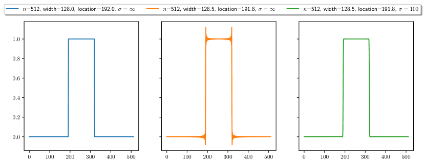
Figure 7: Gaudi Masks in time-domain with different width, location and $\sigma$ on $n=512$. Left: integer width $w=128$ and integer location $l=192$ with $\sigma=\infty$, i.e., no Gaussian smoothing. Middle: non-integer width $w=128.5$ and location $l=191.8$ with $\sigma=\infty$. Due to the non-integer parameters, the time-domain signal contains spiking errors. Right: non-integer width $w=128.5$ and location $l=191.8$ with $\sigma=100$. The Gaussian smoothing in the Gaudi function alleviates the spiking errors.

A.5 More Details on Proximal Gradient Descent on Gaudi-GBLR Parameters in Deep Neural Networks

A.5.1 Discrete Structural Parameters

Here we discuss solving Problem (8) using the discrete width and location parameters $w\in{\mathcal{I}}_{n}$ and $l\in{\mathcal{I}}_{n-1}$. To be specific, given real-valued widths ${\bm{w}}\in[0,n]^{K}$ and locations ${\bm{l}}\in[0,n]^{K}$ of a Gaudi-GBLR matrix, we apply a Straight Through Estimator (Hinton, 2012; Bengio et al., 2013; Zhou et al., 2016) to ${\bm{w}}$ and ${\bm{l}}$ before generating the masks. Then, we project each value of ${\bm{w}}$ and ${\bm{l}}$ to $[0,n]$ after the PGD step. We find that this setting is useful when the Gaussian smoothing parameter $\sigma$ of the Gaudi function is very high or infinite, since the non-integer parameters generate spiking errors as discussed in Appendix A.4.

A.5.2 Multiple Gaudi-GBLR Matrices

For a DNN with $T$ weight matrices, we suggest adjusting the shrinkage parameter $\lambda$ in eq. 9 based on the predefined computational cost budget $B$ for the DNN. For example, one can set $\lambda=0$ if the sum of average widths of the weight matrices $\bar{w}_{\text{sum}}=\bar{w}({\bm{W}}_{1})+\bar{w}({\bm{W}}_{2})+\cdots+\bar{w}({\bm{W}}_{T})$ is below $B$, and use $\lambda=\lambda_{0}>0$ if $\bar{w}_{\text{sum}}$ is above $B$ where $\lambda_{0}$ is given as a hyperparameter by user. In our experiments, this strategy effectively (not necessarily equally) distributes the computational cost to each matrix to meet the overall cost budget constraint during the learning process.

A.6 Extended Experimental Results and Details

A.6.1 Fine-tuning

In fine-tuning experiments, we use the pre-trained ViT-Base (Dosovitskiy et al., 2020). For each pre-trained weight on Query, Key, Value and MLPs, we assign the Gaudi-GBLR matrix where the structural and content parameters are initialized by Algorithm 2. We use the smoothing parameter of the filter $\gamma=1$ and the threshold to obtain the binary mask $\tau=0.98\cdot\max({\bm{c}}_{i_{k}})$ in Eq. 12. During the fine-tuning, we use $\sigma=\infty$ in Eq. 6 Then, all parameters are updated by SGD with AdamW(Loshchilov & Hutter, 2017) optimizers.

For the Block Low-Rank matrices, we use Monarch (Dao et al., 2022) implementation. We project the pre-trained matrix by minimizing the Frobenius norm between the pretrained one and the Monarch matrix by gradient descent for 1000 steps with the learning rate of $0.001$.

The initialization learning rate for the structural parameters was set to $0.0025$ and decayed to $0.000025$. We trained the networks for 35 epochs with the learning rate of $0.0001$ for all parameters, including the structural parameters of the Gaudi-GBLR matrices.

A.6.2 Training from Scratch

For the Gaudi-GBLR matrices, we initialize location parameters to zero and width parameters to the low rank + block sparse structure. The content parameters as well as other weights are initialized randomly.

During the training with Proximal Gradient Descent in Eq. 9, as in Appendix A.5, the shrinkage parameter $\lambda$ is set to zero if the average width of the Gaudi-GBLR matrices of the DNN is below the predefined budget, and recovers the predefined value $\lambda_{0}$ otherwise.

Also, we anneal $\sigma=1$ to $100$ during the training process. $\sigma$ is fixed to $1$ for 5 warm-up epochs, then linearly increases to $100$ for 295 epochs. The hyperparameters used in the ImageNet experiment is presented in Table 3.

Table 3: Hyperparameters used in ImageNet experiments using ViT-Base for training from scratch.

Model	Learning Rate		Shrinkage		$\sigma$ (init/final)	Epochs	Weight Decay	Drop Path Rate
	Structural Params	Content Params	$\lambda_{0}$	Target Width
ViT-Base	N/A	0.001	N/A	N/A	N/A	310	0.05	0.1
ViT-Base Gaudi-GBLR	0.001	0.001	0.04	$0.12\cdot 768$	1.0/100.0	310	0.05	0.0

References

- Amestoy et al. (2015) Patrick Amestoy, Cleve Ashcraft, Olivier Boiteau, Alfredo Buttari, Jean-Yves L’Excellent, and Clément Weisbecker. Improving multifrontal methods by means of block low-rank representations. SIAM Journal on Scientific Computing, 37(3):A1451–A1474, 2015.
- Bengio et al. (2013) Yoshua Bengio, Nicholas Léonard, and Aaron Courville. Estimating or propagating gradients through stochastic neurons for conditional computation. arXiv preprint arXiv:1308.3432, 2013.
- Brown et al. (2020) Tom Brown, Benjamin Mann, Nick Ryder, Melanie Subbiah, Jared D Kaplan, Prafulla Dhariwal, Arvind Neelakantan, Pranav Shyam, Girish Sastry, Amanda Askell, et al. Language models are few-shot learners. Advances in neural information processing systems, 33:1877–1901, 2020.
- Bruckner et al. (1997) Andrew M Bruckner, Judith B Bruckner, and Brian S Thomson. Real analysis. ClassicalRealAnalysis. com, 1997.
- Chen et al. (2022) Beidi Chen, Tri Dao, Kaizhao Liang, Jiaming Yang, Zhao Song, Atri Rudra, and Christopher Re. Pixelated butterfly: Simple and efficient sparse training for neural network models. In International Conference on Learning Representations, 2022. URL https://openreview.net/forum?id=Nfl-iXa-y7R.
- Cooley & Tukey (1965) James W Cooley and John W Tukey. An algorithm for the machine calculation of complex fourier series. Mathematics of computation, 19(90):297–301, 1965.
- Dao et al. (2019) Tri Dao, Albert Gu, Matthew Eichhorn, Atri Rudra, and Christopher Ré. Learning fast algorithms for linear transforms using butterfly factorizations. In International conference on machine learning, pp. 1517–1527. PMLR, 2019.
- Dao et al. (2022) Tri Dao, Beidi Chen, Nimit S Sohoni, Arjun Desai, Michael Poli, Jessica Grogan, Alexander Liu, Aniruddh Rao, Atri Rudra, and Christopher Ré. Monarch: Expressive structured matrices for efficient and accurate training. In International Conference on Machine Learning, pp. 4690–4721. PMLR, 2022.
- Devlin et al. (2018) Jacob Devlin, Ming-Wei Chang, Kenton Lee, and Kristina Toutanova. Bert: Pre-training of deep bidirectional transformers for language understanding. arXiv preprint arXiv:1810.04805, 2018.
- Dosovitskiy et al. (2020) Alexey Dosovitskiy, Lucas Beyer, Alexander Kolesnikov, Dirk Weissenborn, Xiaohua Zhai, Thomas Unterthiner, Mostafa Dehghani, Matthias Minderer, Georg Heigold, Sylvain Gelly, et al. An image is worth 16x16 words: Transformers for image recognition at scale. In International Conference on Learning Representations, 2020.
- Gunasekar et al. (2017) Suriya Gunasekar, Blake E Woodworth, Srinadh Bhojanapalli, Behnam Neyshabur, and Nati Srebro. Implicit regularization in matrix factorization. Advances in neural information processing systems, 30, 2017.
- Hinton (2012) Geoffrey Hinton. Neural networks for machine learning coursera video lectures. 2012.
- Hsu et al. (2022) Yen-Chang Hsu, Ting Hua, Sungen Chang, Qian Lou, Yilin Shen, and Hongxia Jin. Language model compression with weighted low-rank factorization. arXiv preprint arXiv:2207.00112, 2022.
- Huh et al. (2021) Minyoung Huh, Hossein Mobahi, Richard Zhang, Brian Cheung, Pulkit Agrawal, and Phillip Isola. The low-rank simplicity bias in deep networks. arXiv preprint arXiv:2103.10427, 2021.
- Jang et al. (2016) Eric Jang, Shixiang Gu, and Ben Poole. Categorical reparameterization with gumbel-softmax. arXiv preprint arXiv:1611.01144, 2016.
- Jeannerod et al. (2019) Claude-Pierre Jeannerod, Theo Mary, Clément Pernet, and Daniel S Roche. Improving the complexity of block low-rank factorizations with fast matrix arithmetic. SIAM Journal on Matrix Analysis and Applications, 40(4):1478–1496, 2019.
- Kingma & Ba (2014) Diederik P Kingma and Jimmy Ba. Adam: A method for stochastic optimization. arXiv preprint arXiv:1412.6980, 2014.
- Krizhevsky et al. (2009) Alex Krizhevsky, Geoffrey Hinton, et al. Learning multiple layers of features from tiny images. 2009.
- Li et al. (2015) Yingzhou Li, Haizhao Yang, Eileen R Martin, Kenneth L Ho, and Lexing Ying. Butterfly factorization. Multiscale Modeling & Simulation, 13(2):714–732, 2015.
- Lin et al. (2017) Ji Lin, Yongming Rao, Jiwen Lu, and Jie Zhou. Runtime neural pruning. Advances in neural information processing systems, 30, 2017.
- Liu et al. (2018) Hanxiao Liu, Karen Simonyan, and Yiming Yang. Darts: Differentiable architecture search. arXiv preprint arXiv:1806.09055, 2018.
- Loshchilov & Hutter (2017) Ilya Loshchilov and Frank Hutter. Decoupled weight decay regularization. arXiv preprint arXiv:1711.05101, 2017.
- Maddison et al. (2016) Chris J Maddison, Andriy Mnih, and Yee Whye Teh. The concrete distribution: A continuous relaxation of discrete random variables. arXiv preprint arXiv:1611.00712, 2016.
- Pham et al. (2018) Hieu Pham, Melody Guan, Barret Zoph, Quoc Le, and Jeff Dean. Efficient neural architecture search via parameters sharing. In International conference on machine learning, pp. 4095–4104. PMLR, 2018.
- Radford et al. (2019) Alec Radford, Jeffrey Wu, Rewon Child, David Luan, Dario Amodei, Ilya Sutskever, et al. Language models are unsupervised multitask learners. OpenAI blog, 1(8):9, 2019.
- Riad et al. (2022) Rachid Riad, Olivier Teboul, David Grangier, and Neil Zeghidour. Learning strides in convolutional neural networks. In International Conference on Learning Representations, 2022. URL https://openreview.net/forum?id=M752z9FKJP.
- Russakovsky et al. (2015) Olga Russakovsky, Jia Deng, Hao Su, Jonathan Krause, Sanjeev Satheesh, Sean Ma, Zhiheng Huang, Andrej Karpathy, Aditya Khosla, Michael Bernstein, Alexander C. Berg, and Li Fei-Fei. ImageNet Large Scale Visual Recognition Challenge. International Journal of Computer Vision (IJCV), 115(3):211–252, 2015. doi: 10.1007/s11263-015-0816-y.
- Sanh et al. (2020) Victor Sanh, Thomas Wolf, and Alexander Rush. Movement pruning: Adaptive sparsity by fine-tuning. Advances in Neural Information Processing Systems, 33:20378–20389, 2020.
- Tolstikhin et al. (2021) Ilya O Tolstikhin, Neil Houlsby, Alexander Kolesnikov, Lucas Beyer, Xiaohua Zhai, Thomas Unterthiner, Jessica Yung, Andreas Steiner, Daniel Keysers, Jakob Uszkoreit, et al. Mlp-mixer: An all-mlp architecture for vision. Advances in neural information processing systems, 34:24261–24272, 2021.
- Touvron et al. (2021) Hugo Touvron, Matthieu Cord, Matthijs Douze, Francisco Massa, Alexandre Sablayrolles, and Hervé Jégou. Training data-efficient image transformers & distillation through attention. In International conference on machine learning, pp. 10347–10357. PMLR, 2021.
- Vaswani et al. (2017) Ashish Vaswani, Noam Shazeer, Niki Parmar, Jakob Uszkoreit, Llion Jones, Aidan N Gomez, Łukasz Kaiser, and Illia Polosukhin. Attention is all you need. Advances in neural information processing systems, 30, 2017.
- Yaras et al. (2023) Can Yaras, Peng Wang, Wei Hu, Zhihui Zhu, Laura Balzano, and Qing Qu. The law of parsimony in gradient descent for learning deep linear networks. arXiv preprint arXiv:2306.01154, 2023.
- Zhao et al. (2023) Wayne Xin Zhao, Kun Zhou, Junyi Li, Tianyi Tang, Xiaolei Wang, Yupeng Hou, Yingqian Min, Beichen Zhang, Junjie Zhang, Zican Dong, et al. A survey of large language models. arXiv preprint arXiv:2303.18223, 2023.
- Zhou et al. (2016) Shuchang Zhou, Yuxin Wu, Zekun Ni, Xinyu Zhou, He Wen, and Yuheng Zou. Dorefa-net: Training low bitwidth convolutional neural networks with low bitwidth gradients. arXiv preprint arXiv:1606.06160, 2016.
- Zoph & Le (2016) Barret Zoph and Quoc Le. Neural architecture search with reinforcement learning. In International Conference on Learning Representations, 2016.