Threshold detection under a semiparametric regression model

Abstract

Linear regression models have been extensively considered in the literature. However, in some practical applications they may not be appropriate all over the range of the covariate. In this paper, a more flexible model is introduced by considering a regression model $Y=r(X)+\varepsilon$ where the regression function $r(\cdot)$ is assumed to be linear for large values in the domain of the predictor variable $X$. More precisely, we assume that $r(x)=\alpha_{0}+\beta_{0}x$ for $x>u_{0}$, where the value $u_{0}$ is identified as the smallest value satisfying such a property. A penalized procedure is introduced to estimate the threshold $u_{0}$. The considered proposal focusses on a semiparametric approach since no parametric model is assumed for the regression function for values smaller than $u_{0}$. Consistency properties of both the threshold estimator and the estimators of $(\alpha_{0},\beta_{0})$ are derived, under mild assumptions. Through a numerical study, the small sample properties of the proposed procedure and the importance of introducing a penalization are investigated. The analysis of a real data set allows us to demonstrate the usefulness of the penalized estimators.

Keywords : Change point; Model selection; Penalization; Regression models; Regularization; Threshold value.

1 Introduction

Predicting or understanding the structural relationship between a response variable $Y$ based on a scalar explanatory variable $X$ is the primary goal of the so-called regression methods. From the foundational work of Galton, (1886) where simple regression models were introduced, a wide variety of models and estimation procedures have been developed. In this paper, we consider the situation of additive errors, that is we assume that $Y=r(X)+\varepsilon$, where $X$ and $\varepsilon$ are independent random variables and $\mathbb{E}(\varepsilon)=0$ $\mathbb{V}ar(\epsilon)=\sigma^{2}<\infty$.

Parametric and and nonparametric regression models are two main branches where different procedures have been proposed to estimate the regression function $r$. The former usually provide parameter estimators with root-$n$ rates of convergence and predictions easy to interpret, while the latter are more flexible since only some degree of smoothness for the regression function is assumed. Among the first ones, linear regression is one of the most popular models considered among applied practitioners. However, in some situations, the linear assumption does not hold over the whole support of the covariates. To deal with this problem, threshold regression models are commonly used to model some non–linear relationships between the response and the explanatory variable by introducing one or more threshold parameters, also known as change points. Compared with nonparametric regression, threshold regression models are a simple but interpretable alternative, allowing at the same time to provide threshold estimates and inferences. Most of the literature consider that, within each interval defined by the thresholds, the regression function follows a parametric model, generally a linear one. Unlike these models, in this paper the regression function is modelled as linear beyond the threshold, but we do not assume a specific parametric form for the regression function for values of the covariates below the change point. Up to our knowledge, this flexible approach has not been previously considered in the literature.

Even when, in some papers the word threshold has been used to describe regression models where there is no effect on the response before of such a value, throughout this paper no distinction is made between the words threshold or change point to refer to the value where the regression function changes.

We briefly overview some of the contributions done to estimate the regression function when it shows change points. Both, the selection of topics and given references, are far from being exhaustive and we meant to highlight the differences between the existent procedures and our approach to the problem.

Among the pioneering papers in the field, Sprent, (1961) and Bacon and Watts, (1971) considered a two-phase regression model where the regression function is defined by two straight lines, whose slopes and/or intercepts change before and after the threshold. The goal in two-phase regression models or bent line regression ones is to estimate both the coefficients of each linear functions and the threshold. When many thresholds are admitted, allowing for an easy and natural way to gain flexibility in modelling, these models are referred to as segmented regression and most of the proposals were given in piecewise polynomial regression functions with known or unknown change-points. Segmented regression models are very popular in economy, ecology, and medicine, since they permit the practitioner to contemplate different regimes in a unique model, making possible at the same time to estimate where the transitions occur. Their flexibility allowed applications in different disciplines, giving rise to many publications where these techniques have successfully been used. In particular, change point models have provided interesting results modelling Covid data, as shown in Dehning et al., (2020); Coughlin et al., (2021), among others.

Different estimation procedures for segmented regression models have been extensively developed and implemented, among others we can mention Muggeo, (2008, 2017); Fasola et al., (2018); Fong et al., (2017). We also refer to Muggeo, (2003) where a description of procedures to estimate the change points and the regression coefficients is reviewed. As in other regression models, large values of the residuals, associated to the so–called vertical outliers, may affect the estimations. Robust proposals based on ranks have been recently studied by Zhan and Li, (2017) and Shi et al., (2020) for bent line regression and piecewise linear regression models with multiple change points, respectively. Since the first works, presented in Hinkley, (1969) and McZgee and Carleton, (1970), segmented regression models have been extended to many other scenarios and constitute an active area of research. For instance, Muggeo, (2003) and Liang and Zhou, (2008) considered generalized linear segmented models where the natural parameter of the conditional distribution of the response given the explanatory variable is modelled by two straight lines. More general change-point models have received attention from the statistical community over the last decades. Khodadadi and Asgharian, (2008) include a detailed list of papers related to change-points, most of them dealing with situations where the regression is linear in each interval or it is assumed to be 0 before the threshold, meaning that the covariate has no effect on the response if the threshold limit is not exceeded. Change points in time series analysis were studied, among others, in Chan et al., (2015) who considered a threshold autoregressive model with multiple-regimes and introduced a procedure penalizing the autoregressive parameter differences through a LASSO penalty. Threshold models were also studied in high–dimensional settings where variable selection is an important issue, see Lee et al., (2020) who assumes that the regression is linear before and after the change point and penalizes the regression parameters with an adaptive LASSO penalty.

As mentioned above, in this paper we seek for the threshold above which the regression function behaves linearly. Unlike other models considered in the literature, we do not assume a specific form for the regression function for values smaller than the threshold, as done when modelling through piecewise polynomials or bent regression lines. It is worth mentioning that we do not intend to provide estimators for the regression function $r(x)$ on the whole support $[a,b]$ of the covariates, since the goal is to predict responses for large values of the covariates, where it can be assumed that the linear regression model provides a proper fit. In this sense, our approach is more semiparametric than parametric, since it combines a region, let us say $(a,u_{0})$, where no assumptions are made on the shape of the regression function and an interval $[u_{0},b)$ where it is known to be linear. More precisely, for values of the covariates smaller than $u_{0}$, we do not assume that $r(x)$ is known up to a finite number of parameters to be estimated as in the papers mentioned above. For that reason and due to their flexibility, we call the model to be introduced in Section 2 “threshold semiparametric regression model”.

Our motivating example consists of the airquality real data set available in R. The data set corresponds to 153 daily air quality measurements in the New York region between May and September, 1973 (see Chambers et al.,, 1983). The interest is in explaining mean Ozone concentration (“Ozone”, measured in ppb) as a function of the wind speed (“Wind”, in mph). Cleveland, (1985) considered the 111 cases that do not contain missing observations and found that the relationship between ozone concentration and wind speed is non-linear, with higher wind speeds associated to lower Ozone concentrations due to the ventilation that higher speeds bring. We add to his analysis the flexibility of our approach, while maintaining a parametric framework for large values of the covariates. Figure 1 displays the observations together to a nonparametric regression estimator obtained using local polynomials through the function lowess in R, see Cleveland, (1979, 1981).

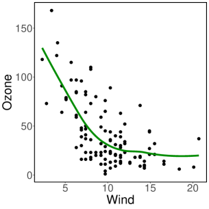
Figure 1: Air quality data (black points) and lowess fit.

The local smoother in Figure 1 suggests that the linear fit is not appropriate all over the support of the covariates, but it may be adequate for large values of the wind speed. In particular, the fit for speeds smaller than 10.5 seems far from a linear one. This motivates the need of providing appropriate estimators of the wind speed from which ozone concentration decreases linearly with wind speed to facilitate predictions. Our approach through threshold semiparametric regression models suits this purpose, since it postulates that the regression function is linear beyond a threshold $u_{0}$ without assuming any parametric form before the change point.

The procedure considered in this paper can easily be adapted to the situation where the model may be assumed to be linear up to an unknown point. This is the case in spectroscopy analysis, where the aim is the determination of the concentration of a compound in a liquid sample, through the measurement of the light absorbed by the solution upon illumination with a lamp. The degree of light absorbed, or absorbance, is related to the concentration of the compound. The Beer-Lambert law establishes that there is a linear relationship between the absorbance and the concentration. However, it is well known that deviations affect the Beer-Lambert equation at high concentrations. The region where these deviations occur are not always evident and depend on the nature of the solution (compound and solvent) and the experimental setting. The identification of the interval with upper limit $u_{0}$, where the linear relation may be assumed is therefore very important for an accurate quantification and it is usually determined graphically from a calibration plot. The threshold semiparametric regression model and the penalized threshold estimator to be considered provides a less visual dependent tool to estimate $u_{0}$.

The threshold regression semiparametric model provides a simple and easily interpretable model, since it allows to obtain the threshold above which the regression function may assumed to be linear. In both examples described above obtaining this unknown change–point becomes crucial. To provide a consistent estimator of the threshold, we introduce a penalty function which penalizes large values of the threshold. This is another of the novelties of the paper, since up to our knowledge, penalties have only been considered to penalize the linear regression parameters but not the change point candidates.

In the rest of the paper we will introduce the model, the estimators of the threshold $u_{0}$ and we will study some of its properties. The paper is organized as follows. Section 2.1 describes the threshold regression semiparametric model and provides a characterization of the threshold that will be a key point to define the estimators which are introduced in Section 2.2. Section 3 summarize the asymptotic properties of the proposed estimators including consistency results for the estimators of the threshold and of the intercept and slope regression function assumed beyond $u_{0}$. Asymptotic normality results are also derived for the linear regression coefficient estimators obtained for values larger than $\widehat{u}+\psi$, where $\widehat{u}$ is the estimated threshold and $\psi>0$. Section 4 reports the results of a Monte Carlo study conducted to examine the small sample properties of the proposed procedure for different sample sizes according to the penalization constant, the values of the threshold and the regression smoothness. The usefulness of the proposed methodology is illustrated in Section 5 on a real data set, while some final comments are presented in Section 6. All proofs are relegated to the Appendix.

2 The threshold and its estimation

2.1 The threshold regression semiparametric model

Let $X$ and $Y$ be squared integrable random variables taking values in $\mathbb{R}$, satisfying the regression model

$$Y=r(X)+\varepsilon\;,$$ (1)

where $X$ and $\varepsilon$ are independent random variables and the error term $\varepsilon$ has mean zero and finite variance $\sigma^{2}$. Denote ${\mathcal{S}}$ the support of the random variable $X$ and assume that ${\mathcal{S}}=[a,b]$, i.e., ${\mathcal{S}}$ is a connected set, where $a$ and $b$ may be infinite.

In this paper, we deal with the situation where the regression function $r(x)$ is linear for values $x$ of the covariate large enough; namely, $r(x)=\alpha+\beta\,x$ for $x>u$, $x\in{\mathcal{S}}$. Let $u_{0}$ denotes the smallest value of $u$ above which $r(x)$ is linear. More precisely, define the threshold $u_{0}$ as

$$u_{0}=\inf\{u\in{\mathcal{S}}:\hbox{$u<b$ and for some}\;\alpha,\beta\in\mathbb{R}\quad\mathbb{P}(r(X)=\alpha+\beta\,X\mid X>u)=1\}=\inf{\mathcal{U}}\;.$$ (2)

If ${\mathcal{U}}$ is empty, then $u_{0}=+\infty$. However, assumption C3 below avoids this case. The possible values of $u$ in (2) are restricted to be in the support of the covariate to avoid an spurious threshold in the situation where the regression function is linear all over the support and $a\neq-\infty$. In such a case, with the above definition $u_{0}=a$, while if the set ${\mathcal{U}}$ allows for any $u\in\mathbb{R}$, the infimum of ${\mathcal{U}}$ would have been $-\infty$.

It is also worth mentioning that if $\widetilde{u}\in{\mathcal{U}}$, then any $u$ such that $u>\widetilde{u}$ is also an element of ${\mathcal{U}}$ and the regression function related to $u$ will have the same coefficients as the one defined by $\widetilde{u}$. This fact implies that, when ${\mathcal{U}}$ is not empty, whether $u_{0}=-\infty$ or $u_{0}$ belongs to ${\mathcal{U}}$ meaning that the infimum in (2) is indeed a minimum. For covariates with unbounded support, the situation $u_{0}=-\infty$ arises when the regression model is linear, i.e., when there exists $\alpha_{0},\beta_{0}\in\mathbb{R}$ such that $\mathbb{P}(r(X)=\alpha_{0}+\beta_{0}\,X)=1$. When $u_{0}\neq-\infty$, taking into account that $u_{0}$ belongs to ${\mathcal{U}}$, we also denote $\alpha_{0},\beta_{0}\in\mathbb{R}$ the values such that $\mathbb{P}(r(X)=\alpha_{0}+\beta_{0}\,X\mid X>u_{0})=1$, implying that $\mathbb{P}(r(X)=\alpha_{0}+\beta_{0}\,X\mid X>u)=1$, for any $u\geq u_{0}$.

The aim of this work is to estimate the threshold $u_{0}$ when it is finite on the basis of an i.i.d. sample ${\mathcal{Z}}_{n}=\{Z_{i}=(X_{i},Y_{i}),1\leq i\leq n\}$, distributed as $(X,Y)$, following a model selection approach. To do so, we first define a function allowing to characterize the threshold $u_{0}$. In the sequel, we assume that $u_{0}<+\infty$ and that the distribution function $F_{X}$ of $X$ is continuous. In this way, probabilities and expectations conditioned on $\{X>u\}$ or on $\{X\geq u\}$ agree. Furthermore, to simplify the notation, when $u_{0}=-\infty$ conditioning on $\{X>u_{0}\}$ or on $\{X\geq u_{0}\}$ means that no conditions are imposed when conditioning.

We first begin by defining the best linear predictor of the responses when considering only large values of the covariates. More precisely, for each $u\in\mathbb{R}$ with $u<b$, define $(\alpha_{u},\beta_{u})$ as the best coefficients to linearly predict $Y$ based on $X$, when $X\geq u$, that is,

$$(\alpha_{u},\beta_{u})=\mathop{\mbox{argmin}}_{\alpha,\beta}\;\mathbb{E}\left[\left\{Y-(\alpha+\beta\,X)\right\}^{2}\mid X\geq u\right]\,.$$ (3)

Some facts should be highlighted regarding the coefficients $(\alpha_{u},\beta_{u})$. When $u_{0}\neq-\infty$, given $u\geq u_{0}$, under C1 below, we have that $(\alpha_{u},\beta_{u})$ is constant and equal to $(\alpha_{0},\beta_{0})$. Moreover, when $u_{0}=-\infty$, we also have that $(\alpha_{0},\beta_{0})=(\alpha_{u},\beta_{u})$ for any $u<b$, since $\mathbb{P}(r(X)=\alpha_{0}+\beta_{0}\,X)=1$.

To show the first assertion, recall that, when $u_{0}\neq-\infty$, $\mathbb{P}(r(X)=\alpha_{0}+\beta_{0}\,X\mid X\geq u)=1$, for any $u\geq u_{0}$, since we are assuming that $F_{X}$ is continuous. Hence, when $\mathbb{E}(\epsilon)=0$ as stated in C1, the independence between the errors and the covariates entail that

$$\mathbb{E}\left[\left\{Y-(\alpha+\beta\,X)\right\}^{2}\mid X\geq u\right] =\mathbb{E}\left[\left\{r(X)-(\alpha+\beta\,X)\right\}^{2}\mid X\geq u\right]+\mathbb{E}(\epsilon^{2})$$

$$=\mathbb{E}\left[\left\{\alpha_{0}+\beta_{0}\,X-(\alpha+\beta\,X)\right\}^{2}\mid X\geq u\right]+\mathbb{E}(\epsilon^{2})\,.$$

Therefore, for $u\geq u_{0}$, the minimum of $\mathbb{E}\left[\left\{Y-(\alpha+\beta\,X)\right\}^{2}\mid X\geq u\right]$ is attained at $(\alpha_{u},\beta_{u})$ when $\mathbb{P}\left((\alpha_{0}-\alpha_{u})+(\beta_{0}-\beta_{u})\,X=0\mid X\geq u\right)=1$. The continuity of $F_{X}$, allow to conclude that $(\alpha_{u},\beta_{u})=(\alpha_{0},\beta_{0})$, as desired.

To characterize the threshold $u_{0}$, consider the loss function defined, for $u<b$, as

$$\ell(u)=\mathbb{E}[\{Y-(\alpha_{u}+\beta_{u}X)\}^{2}\mid X\geq u)]=\frac{\mathbb{E}\left[\{Y-(\alpha_{u}+\beta_{u}X)\}^{2}\mathbb{I}_{\{X\geq u\}}\right]}{\mathbb{P}(X\geq u)}.$$ (4)

It is worth noticing that $\ell(u)$ depends on $F$, the joint distribution of $Z=(X,Y)$, i.e, we should have used $\ell(u,F)$ to reinforce this dependence in lieu of $\ell(u)$, but we have decided to omit the dependence on $F$ to simplify the notation.

One important issue to be considered when defining an estimator is if it is indeed estimating the target quantity, in our case, $(u_{0},\alpha_{0},\beta_{0})$. This property, known as Fisher–consistency, is usually a first step before obtaining consistency results. When the estimator can be written as a functional applied to the empirical distribution, this property has an easy representation, see for instance Huber and Ronchetti, (2009). Even in our case, where penalized estimators will be considered, the first step before defining them is to ensure that the function $\ell(\cdot)$ allows to characterize $u_{0}$; this fact is related to the Fisher–consistency property described above. However, in our situation the function $\ell(\cdot)$ will not have a unique minimum but will be constant for values larger than $u_{0}$. Hence, the estimators to be defined below need to take into account this fact and to search for the “smallest” value where the minimum of the empirical counterpart of $\ell(u)$ is attained. The penalty function to be introduced will be important to achieve this goal.

The following set of assumptions will be needed in the sequel

1. The errors and covariates are such that $\mathbb{E}(X^{2})<\infty$, $\mathbb{E}(\varepsilon^{2})<\infty$ and $\mathbb{E}(\varepsilon)=0$.

2. The distribution function $F_{X}$ of the random variable $X$ is continuous.

3. The threshold $u_{0}$ defined in (2) is finite, i.e., $u_{0}<+\infty$.

4. The threshold $u_{0}$ defined in (2) is such that $u_{0}\neq a$, that is, for any $\alpha,\beta\in\mathbb{R}$, $\mathbb{P}(r(X)=\alpha+\beta\,X)<1$.

Conditions C3 and C4 establish the semiparametric nature of the model postulated in this paper: above the threshold $u_{0}$ the regression is assumed to be linear, but below it, no specific form is assumed for the relation between the response and the covariate.

Lemma 2.1 states the characterization of the threshold $u_{0}$ in terms of the loss function $\ell(u)$.

Lemma 2.1.

Let $(Y,X)$ be a random vector satisfying (1) and let $u_{0}$ be defined as in (2). Assume that C1 to C3 hold. Then,

1. The function $\ell:(-\infty,b)\to\mathbb{R}$ defined by (4) is continuous.

2. Define $\ell(u_{0})=\mathbb{E}(\varepsilon^{2})$ when $u_{0}=-\infty$. Then,

   $$\ell(u_{0})=\ell(u)\;\hbox{for all $u$ such that $u_{0}\leq u<b$}.$$ (5)

3. If in addition C4 holds, we also have that

   $$\ell(u)>\ell(u_{0})\hbox{ for all $u<u_{0}$ }\,.$$ (6)

4. If in addition C4 holds, for any $\delta>0$, we have that

   $$\inf_{u\leq u_{0}-\delta}\ell(u)>\ell(u_{0})\,.$$ (7)

2.2 The estimators

The characterization of the threshold $u_{0}$ presented in equations (5) and (6) of Lemma 2.1 implies that, for any $\lambda>0$ and any positive and increasing function $f$, the minimum of $\ell(u)+\lambda\,f(u)$ on $[u_{0},b)$ is achieved when $u=u_{0}$. This suggests that the threshold can be estimated combining an estimator of the loss function $\ell(\cdot)$ with a penalization term. The behaviour of $\ell(u)+\lambda\,f(u)$ on $[u_{0},b)$ clarifies why the penalization is needed to avoid estimating the threshold with large values, which could be induced as a natural consequence of an over-fitting phenomena.

Throughout the paper, to shorten the expressions below, we will use a notation closely related to the one used in empirical processes. Let $(X_{i},Y_{i})$, $1\leq i\leq n$, be i.i.d. observations, $\mathbb{P}_{n}$ stands for the empirical mean operator

$$\mathbb{P}_{n}(g(X,Y))=\frac{1}{n}\sum_{i=1}^{n}g(X_{i},Y_{i})\,,$$

which is the empirical counterpart of $\mathbb{P}(g(X,Y))=\mathbb{E}(g(X,Y))$.

Given a sample $\mathcal{Z}_{n}=\{Z_{i}=(X_{i},Y_{i}),1\leq i\leq n\}$ distributed as $(X,Y)$, to define an estimator of $\ell$, we first introduce estimators $(\widehat{\alpha}_{u},\widehat{\beta}_{u})$ of $(\alpha_{u},\beta_{u})$ by considering the least squares regression estimators for the regression of $Y$ on $X$ using only those observations with $X_{i}\geq u$, that is,

$$(\widehat{\alpha}_{u},\widehat{\beta}_{u})=\mathop{\mbox{argmin}}_{\alpha,\beta}\mathbb{P}_{n}\left\{\left(Y-\alpha-\beta X\right)^{2}\mathbb{I}_{\{X\geq u\}}\right\}\,.$$ (8)

We now consider the estimator $\widehat{\ell}(u,{\mathcal{Z}}_{n})$ of $\ell(u)$ given by

$$\widehat{\ell}(u,{\mathcal{Z}}_{n})=\frac{\mathbb{P}_{n}\left[\left\{Y-(\widehat{\alpha}_{u}+\widehat{\beta}_{u}X)\right\}^{2}\mathbb{I}_{\{X\geq u\}}\right]}{\mathbb{P}_{n}\left(\mathbb{I}_{\{X\geq u\}}\right)}\,.$$ (9)

Remark 2.1.

Two facts should be mentioned regarding the estimator $\widehat{\ell}$. The first observation is related to its numerical evaluation. Notice that, as a function of $u$, $\widehat{\ell}(u,{\mathcal{Z}}_{n})$ is constant between consecutive sample predictor values. Therefore, to compute the loss function it is enough to evaluate $\widehat{\ell}(u,{\mathcal{Z}}_{n})$ only on the sample points and not on the entire domain of the distribution, reducing the numerical complexity. Furthermore, for any $u<\min_{1\leq i\leq n}X_{i}$, we have that $\widehat{\ell}(u,{\mathcal{Z}}_{n})=\sum_{i=1}^{n}r_{i}^{2}/n$, where $r_{i}=Y_{i}-(\widehat{\alpha}+\widehat{\beta}X_{i})$ and $(\widehat{\alpha},\widehat{\beta})$ is the least squares estimators of the coefficients of a simple regression model using the complete sample.

The second one regards the proper definition of $\widehat{\ell}$. When estimating the denominator $\mathbb{P}(X\geq u)$ in $\ell$ by its empirical counterpart $\mathbb{P}_{n}\left(\mathbb{I}_{\{X\geq u\}}\right)=\#\{X_{i}\geq u\}/n$, we have to take into account that some fraction of points lying at the right-hand side of $u$ is needed to guarantee that $\mathbb{P}_{n}(\mathbb{I}_{\{X\geq u\}})>0$. Hence, only values of $u$ smaller than the maximum of the sample are allowed. This is similar to the fact that $\ell(u)$ is finite for values of $u$ smaller than $b$. However, to define a consistent estimator of the threshold using the characterization provided by (5), we will need to upper bound the possible sets of values for $u$. More precisely, we will assume below that for some $0<\eta_{1}<1$, the threshold $u_{0}$ is small than the $1-\eta_{1}$ quantile of the covariates distribution, $\gamma=F_{X}^{-1}(1-\eta_{1})$. Furthermore, we will denote as $\gamma_{n}$ the corresponding empirical quantile, that is, we ensure that $\mathbb{P}_{n}(\mathbb{I}_{\{X\geq u\}})\geq\eta_{1}$ for all $u\leq\gamma_{n}$.

To define the objective function allowing to estimate $u_{0}$, we add a penalization term to the empirical loss function $\widehat{\ell}(u,{\mathcal{Z}}_{n})$ and define

$$\mathrm{PL}(u,{\mathcal{Z}}_{n})=\widehat{\ell}(u,{\mathcal{Z}}_{n})+\lambda_{n}f(u)\,,$$ (10)

where $f$ is a non–negative and non–decreasing function. The threshold estimator $\widehat{u}_{n}$ is defined as

$$\widehat{u}_{n}=\mathop{\mbox{argmin}}_{u:u\leq\gamma_{n}}\,\mathrm{PL}(u,{\mathcal{Z}}_{n}).$$ (11)

Observe that $\widehat{u}_{n}$ satisfies

$$\mathrm{PL}(\widehat{u}_{n},{\mathcal{Z}}_{n})\;\leq\;\mathrm{PL}(u,{\mathcal{Z}}_{n})\;,\quad\hbox{for all $u\leq\gamma_{n}$}.$$

3 Asymptotic properties

To derive consistency results for the threshold estimators $\widehat{u}_{n}$ and for the linear regression estimators $(\widehat{\alpha}_{\widehat{u}},\widehat{\beta}_{\widehat{u}})$, where $(\widehat{\alpha}_{u},\widehat{\beta}_{u})$ is defined in (8), we will need the following additional assumptions.

1. For some $0<\eta_{1}<1$, $\gamma=F_{X}^{-1}(1-\eta_{1})>u_{0}$ and $\gamma_{n}$ is the $1-\eta_{1}$ empirical quantile of $X_{1},\dots,X_{n}$.

2. The function $f:\mathbb{R}\to\mathbb{R}$ is a non–negative, non–decreasing function, strictly increasing in a neighbourhood of $u_{0}$.

3. The covariates and responses are such that $\mathbb{E}(X^{2}Y^{2})<\infty$.

Remark 3.1.

As mentioned above assumption C5 prevents the denominator $\mathbb{P}_{n}\left(\mathbb{I}_{\{X\geq u\}}\right)$ to be equal to 0. Clearly, under C5 assumption C3 holds, for that reason in the results below we omit assumption C3 in their statements. It is also worth mentioning that C3 entails that $\mathbb{P}(r(X)=\alpha_{0}+\beta_{0}\,X\,\mid\,X\geq u_{0})=1$, moreover, $\mathbb{P}(r(X)=\alpha_{0}+\beta_{0}\,X\,\mid\,X\geq u)=1$ for any $u\geq u_{0}$.

Assumption C6 holds when $f$ is strictly increasing on the support ${\mathcal{S}}$ of $X$. One possible choice for $f$ is to consider $f(u)=\arctan(u)$. When $a\neq-\infty$, we can also select $f(u)=u-a$ for $u\geq a$ and $0$ otherwise, that corresponds to the penalizing function selected in our numerical study and in the real data analysis.

Condition C1 is a standard assumption when considering least squares regression estimators. Assumption C7 is needed to ensure that $\widehat{\beta}_{u}-{\beta}_{u}$ has a root-$n$ rate of convergence, uniformly on $u\leq F_{X}^{-1}(1-\eta)$, with $\eta>0$, as stated in Lemma A.2. Note that for values of $u<u_{0}$, the regression function is not linear and for that reason a stronger moment requirement than the usual for linear regression models is needed. From the Cauchy Schwartz inequality we obtain that assumption C7 holds when $\mathbb{E}(X^{4})<\infty$ and $\mathbb{E}(Y^{4})<\infty$.

It is also worth mentioning that C7 is a consequence of C1 when the regression function $r$ is bounded on the support of $X$. For instance, if ${\mathcal{S}}$ is bounded and the regression function $r$ is continuous, assumption C1 implies assumption C7. Hence, if $r$ is bounded on ${\mathcal{S}}$, C7 may be omitted in the statement of Theorems 3.1 and 3.3 and in Corollary 3.2.

Theorem 3.1 below states that the least squares penalized loss gives rise to a consistent estimator of the threshold $u_{0}$. However, consistency results for threshold estimator are not restricted to the specific loss function given by (4) and its empirical counterpart given by (9) if a penalty term is included as in (10). Any continuous loss function characterizing the threshold through (5) and any reasonable estimator of such a loss function, such as its empirical counterpart, would work as well, as shown in Proposition 3.1.

Proposition 3.1.

Let $(X,Y)$ be a random vector of squared integrable variables satisfying the regression model (1) and let $u_{0}$ be defined as in (2). Consider a continuous loss function $\ell:(-\infty,b)\to\mathbb{R}$ satisfying (5), (6) and (7). Define $\mathrm{PL}(u,{\mathcal{Z}}_{n})$ as in (10), where the function $f$ satisfies C6 and the function $\widehat{\ell}(u,{\mathcal{Z}}_{n})$ is such that

1. $\sup_{\{u\colon u\leq u_{0}\}}|\widehat{\ell}(u,{\mathcal{Z}}_{n})-\ell(u)|\buildrel p\over{\longrightarrow}0$.

2. For some sequence $a_{n}$ converging to zero and for any $\widetilde{\gamma}=F_{X}^{-1}(1-\eta)$ with $\eta>0$

   $$\lim_{n\to\infty}\mathbb{P}\left(\sup_{u\in[u_{0},\widetilde{\gamma}]}|\widehat{\ell}(u,{\mathcal{Z}}_{n})-\ell(u)|\leq a_{n}\right)=1\,.$$

Let $\widehat{u}_{n}$ be defined through (11). Then, under C1, C2 and C5, if the sequence $\lambda_{n}>0$ is such that $\lambda_{n}\to 0$ and $a_{n}/\lambda_{n}\to 0$ when $n\to\infty$, we have that $\widehat{u}_{n}\buildrel p\over{\longrightarrow}u_{0}$.

As mentioned above Theorem 3.1 establishes the consistency of the threshold estimators when using the squared loss function.

Theorem 3.1.

Assume $\{(X_{i},Y_{i}):i\geq 1\}$ are i.i.d., distributed as $(X,Y)$ satisfying the regression model (1) and let $u_{0}$ be defined as in (2). Assume that C1, C2 and C4 to C7 hold. Let $\widehat{u}_{n}$ be defined as in (11) and $\widehat{\ell}(u,{\mathcal{Z}}_{n})$ defined in (9). Then, if $\lambda_{n}\to 0$, and there exists $\varphi_{n}\to+\infty$, such that $n^{1/2}\lambda_{n}/\varphi_{n}\to+\infty$, we have that $\widehat{u}_{n}\buildrel p\over{\longrightarrow}u_{0}$.

Note that as a consequence of Theorem 3.1 $\widehat{u}_{n}\buildrel p\over{\longrightarrow}u_{0}$, when the penalty parameter $\lambda_{n}$ converges to $0$ with almost root-$n$ rates, as in the following two cases: $\lambda_{n}=cn^{-\xi}$ for some $0<\xi<1/2$, or $\lambda_{n}=c\,n^{-1/2}\,\log(n)$, since it is enough to choose $\varphi_{n}=n^{-\omega}$ with $\xi+\omega<1/2$ or $\varphi_{n}=\log(\log n)$, respectively.

An important issue is to show that the least squares estimators obtained using only the observations larger the consistent threshold $\widehat{u}_{n}$ provide consistent estimators of the true parameters $\alpha_{0},\beta_{0}$. Following the notation introduced in (8), $\widehat{\alpha}_{\widehat{u}}$ and $\widehat{\beta}_{\widehat{u}}$ stand for the least squares estimators of the intercept and slope when the sub-sample $\{(X_{i},Y_{i}):X_{i}\geq\widehat{u}_{n}\}$ is used in the estimation process.

Corollary 3.2.

Assume $\{(X_{i},Y_{i}):i\geq 1\}$ are i.i.d., distributed as $(X,Y)$ satisfying the regression model (1) and let $u_{0}$ be defined as in (2). Under C1, C2 and C4 to C7, we have that $(\widehat{\alpha}_{\widehat{u}},\widehat{\beta}_{\widehat{u}})\buildrel p\over{\longrightarrow}(\alpha_{0},\beta_{0})$.

Theorem 3.3 provides an asymptotic normality result for the intercept and slope regression coefficients obtained using the observations with $X_{i}\geq\widehat{u}+\psi$, for any $\psi>0$. More precisely, it shows that given $\psi>0$, $(\widehat{\alpha}_{\widehat{u}+\psi},\widehat{\beta}_{\widehat{u}+\psi})$ asymptotically behaves as the estimators computed using the threshold $u_{0}+\psi$, which are asymptotically normal according to the well known results for weighted least squares regression estimators. First recall that for any $\psi>0$, $\alpha_{u_{0}+\psi}=\alpha_{u_{0}}$ and $\beta_{u_{0}+\psi}=\beta_{u_{0}}$, so Lemma A.2 and the continuity of $\alpha_{u}$ and $\beta_{u}$ stated in the proof of Lemma 2.1 implies that $(\widehat{\alpha}_{\widehat{u}+\psi},\widehat{\beta}_{\widehat{u}+\psi})\buildrel p\over{\longrightarrow}(\alpha_{0},\beta_{0})$.

Theorem 3.3.

Assume $\{(X_{i},Y_{i}):i\geq 1\}$ are i.i.d., distributed as $(X,Y)$ satisfying the regression model (1) and let $u_{0}$ be defined as in (2). Assume that C1, C2 and C4 to C7 hold and that $\widehat{u}_{n}\buildrel p\over{\longrightarrow}u_{0}$. Then, for any fixed positive constant $\psi$ we have that

$$\sqrt{n}\{(\widehat{\alpha}_{\widehat{u}+\psi},\widehat{\beta}_{\widehat{u}+\psi})-(\alpha_{0},\beta_{0})\}\buildrel D\over{\longrightarrow}{\mathcal{N}}(0,\mbox{\boldmath$\Sigma$}_{u_{0}+\psi})\,,$$

where $\mbox{\boldmath$\Sigma$}_{u_{0}+\psi}=\sigma^{2}\left\{\mathbb{E}\left(\mathbb{I}_{\{X\geq u_{0}+\psi\}}\widetilde{\mathbf{X}}\widetilde{\mathbf{X}}^{\top}\right)\right\}^{-1}$ with $\widetilde{\mathbf{X}}=(1,X)^{\top}$.

4 Monte Carlo study

In this section, we report the results of a small simulation study conducted to numerically explore the finite sample behaviour of the estimators defined in Section 2. We aim to compare our proposal with the estimators obtained minimizing $\widehat{\ell}(u,{\mathcal{Z}}_{n})$ to illustrate that some degree of penalization is needed to obtain a consistent procedure. One of the goals of this numerical study is also to show the effect that the penalization term, the errors scale and the smoothness of the regression function may have on the threshold estimators.

The threshold estimator was computed using the definition given through (11), taking as $\gamma_{n}$ the 95% empirical quantile of the predictors. In all scenarios, the penalty parameter was defined as $\lambda_{n}=cn^{-0.4}$ for different values of the constant $c>0$ and the function $f$ equals the identity function in $[0,1]$, i.e., we chose $f(u)=u$ for $u\geq 0$ and $f(u)=0$ for $u<0$. Note that the non–penalized case corresponds to $c=0$ and is included to show that, in this case, the threshold estimator does not converge to the true regression function threshold. It is worth mentioning that according to Theorem 3.1, the penalty parameter $\lambda_{n}$ should converge to $0$ with a rate slower than $\sqrt{n}$ to ensure consistency, for that reason we have chosen $\lambda_{n}=cn^{-0.4}$.

To provide a broad comparison, we considered different regression functions depending on the threshold value $u_{0}$ and also on a constant $\delta$ which allows us to include functions which are not differentiable at $u_{0}$. We also studied different scenarios according to the errors standard deviations and to the sample size. In all cases, we performed $Nrep=1000$ replications.

To define the regression function, let us denote as $g:[0,1]\to\mathbb{R}$ the non-linear function defined as

$$g(x)=\left\{\begin{array}[c]{lll}4x^{2}(3-4x)&&\text{if $0\leq x\leq 0.5$}\,,\\ &&\\ \displaystyle{\frac{4}{3}}\,x\,(4x^{2}-10x+7)-1&&\text{if $0.5\leq x\leq 1$}\,.\end{array}\right.$$

The family of regression functions will be labelled according to the threshold value $u_{0}$ and to the smoothing parameter $\delta\in\mathbb{R}$ involved in its definition, that is, we denote as $r_{u_{0},\delta}:[0,1]\to\mathbb{R}$, the function

$$r_{u_{0},\delta}(x)=\left\{\begin{array}[c]{lll}g(x)&&\text{if $0\leq x\leq u_{0}$}\,,\\ &&\\ \{g^{\prime}(u_{0})+\delta\}(x-u_{0})+g(u_{0})&&\text{if $u_{0}\leq x\leq 1$}\,.\end{array}\right.$$

It is worth mentioning that regardless of the value of $\delta$, the function $r_{u_{0},\delta}(x)$ is continuous. However, it is only differentiable at $u_{0}$ when $\delta=0$. Note that when $u_{0}=0.5$, $g(u_{0})=1$ and $g^{\prime}(u_{0})=0$. Hence for $u_{0}=0.5$ and $\delta=0$, the function $r_{u_{0},\delta}(x)$ is constant on $[u_{0},1]$, while for any $\delta$, on $[0,u_{0}]$, $r_{u_{0},\delta}(x)=4x^{2}(3-4x)$. Figure 2 shows the plots of $g(x)$ and the regression function $r_{u_{0},\delta}(x)$ for different values of $u_{0}$ and $\delta$.

$g(x)$	$u_{0}=0.5$, $\delta=0$	$u_{0}=0.5$, $\delta=\,-\,1$
$u_{0}=0.75$, $\delta=1$	$u_{0}=0.75$, $\delta=0$	$u_{0}=0.75$, $\delta=\,-\,1$

Figure 2: Plot of the function $g(x)$ (upper left panel) and of the regression function $r_{u_{0},\delta}(x)$ for different values of the threshold $u_{0}$ and smoothing parameter $\delta$.

For each replication, we generate independent samples $(X_{i},Y_{i})\sim(X,Y)$, $i=1,\dots,n$, where $X\sim{{\mathcal{U}}}(0,1)$ and $Y=r_{u_{0},\delta}(X)+\varepsilon$, with $\varepsilon\sim{\mathcal{N}}(0,\sigma^{2})$, independent of $X$. Note that for any value of $\delta$, the observations satisfy the postulated model (1) with $b=g^{\prime}(u_{0})+\delta$, $a=g(u_{0})-b\,u_{0}$ and threshold at $u_{0}$ as defined in (2). Across the different scenarios, we vary the sample sizes from $n=100$ to $n=2000$ with step=100. Two values for $u_{0}$ were selected to illustrate the performance of the proposed procedure $u_{0}=0.5$ and $u_{0}=0.7$ combined with three values for $\delta$, $\delta=-1,0$ and $1$. In this way we get six different scenarios for the regression function $r_{u_{0},\delta}$, defined in (1). Finally, three values for the errors standard deviation were selected, $\sigma=0.01,0.05$ and $0.1$.

To illustrate the structure of the different data sets obtained as $u_{0}$ and $\delta$ vary, Figure 3 displays one of the pairs $(X_{i},Y_{i})$, $i=1,\dots,n$, obtained when $n=50$ together with the regression function $r_{u_{0},\delta}$ used to generate them. Note that when $u_{0}=0.75$ the linear relationship becomes more evident as the absolute value of $\delta$ increases,. As shown below, this fact will be also confirmed by our numerical results.

$u_{0}=0.5$, $\delta=0$	$u_{0}=0.5$, $\delta=\,-\,1$	$u_{0}=0.5$, $\delta=1$
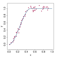
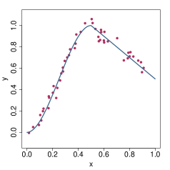
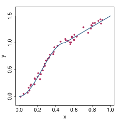
$u_{0}=0.75$, $\delta=0$	$u_{0}=0.75$, $\delta=\,-\,1$	$u_{0}=0.75$, $\delta=1$

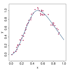
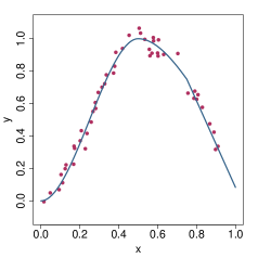
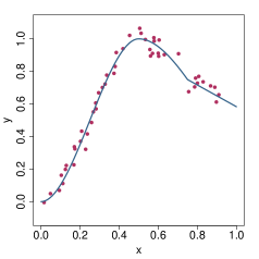
Figure 3: Datasets with $n=50$ observations generated through the model (1) with different regression functions $r_{u_{0},\delta}(x)$ from Figure 2 and $\epsilon\sim\mathcal{N}(0,0.05^{2})$.

To evaluate the performance of the estimators, we computed the empirical mean absolute error (EMAE) of the estimator over replications defined as

$$\hbox{{EMAE}}=\frac{1}{Nrep}\sum_{s=1}^{Nrep}|\widehat{u}^{s}_{n}-u_{0}|,$$ (12)

where $\widehat{u}_{n}^{s}$, $s=1\ldots,Nrep$, stands for the estimate obtained at the $s$-th replication when the sample size equals $n$ and when the regression function equals $r_{u_{0},\delta}$. Clearly, the obtained value of EMAE varies across the studied scenarios depending on each combination of $u_{0}$, $\delta$, $\sigma$, $n$ and $c$.

$c=0$	$c=0.005$
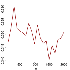
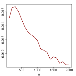
$c=0.10$	$c=0.05$

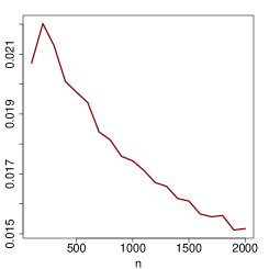
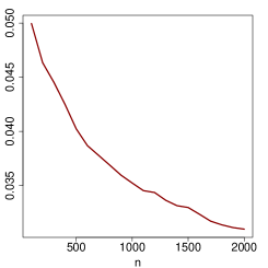
Figure 4: Behaviour of EMAE as a function of $n$ for different values of $c>0$ when the penalty parameter equals $\lambda_{n}=cn^{-0.4}$. In all cases, $u_{0}=0.5$, $\delta=-1$ and $\sigma=0.01$.

To evaluate the behaviour of the threshold estimate as the sample size increases, Figure 4 presents the plots of the empirical mean absolute error as $n$ increases for $c=0,0.005,0.01$ and $0.05$. In the four situations represented, the error standard deviation equals $\sigma=0.01$ and the regression function corresponds to $r_{u_{0},\delta}(x)$ with $u_{0}=0.5$ and $\delta=-1$. Figure 4 confirms the consistency result stated in Theorem 3.1 when penalizing the objective function. Effectively, for any $c>0$, the EMAE decreases with $n$ showing that $\widehat{u}_{n}\to u_{0}$ when $n\to\infty$. In contrast, when $c=0$ the empirical mean absolute error has an erratic behaviour as the sample size increases, showing that the penalizing term is necessary for the consistency of the estimator.

$r_{u_{0},\delta}(x)$, $u_{0}=0.5$, $\delta\,=\,-\,1$
a)	b)
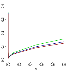
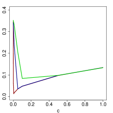
$r_{u_{0},\delta}(x)$, $u_{0}=0.75$, $\delta\,=\,-\,1$
c)	d)

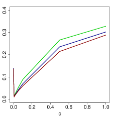
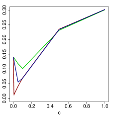
Figure 5: Plot of EMAE as a function of the penalizing constant $c$ for two regression functions. The a) and c) panels correspond to $\sigma=0.01$ and the green, blue and red lines represent the EMAE for $n=500,1000$ and $1500$. The b) and d) panels correspond to $n=1000$ and the solid green, blue and red lines correspond to $\sigma=0.10,0.05$ and $0.01$, respectively.

Taking into account that the estimators performance may depend on the penalizing constant $c$, we also explore the behaviour of EMAE for different sample sizes and values of the errors standard deviation as a function of $c$, when $c$ varies between $0$ and $1$ taking the values 0, $10^{-k}$ and $0.5\times 10^{-k}$, for $k=0,\ldots,10$. Figure 5 displays the empirical mean absolute error for $c\in[0,1]$. The left panels correspond to $\sigma=0.01$ with the green, blue and red lines representing the EMAE for three sample sizes $n=500,1000$ and $1500$. The plots on the right panels represent EMAE when the sample size equals $n=1000$ and three values of the standard error. In this case, the solid green, blue and red lines correspond to $\sigma=0.10,0.05$ and $0.01$, respectively. Figure 5 clearly shows that, as expected, a discontinuity in the empirical mean absolute error occurs at $c=0$, since for that value of the penalty parameter the threshold estimator does not converge to the true threshold. Besides, even when the estimators are consistent for any $c>0$, the EMAE increases with $c$ for the sample sizes and standard errors considered, since in this case, the penalty tends to dominate over the objective function $\widehat{\ell}(u,{\mathcal{Z}}_{n})$. The plots reveal that there is an optimal value for the constant $c$, that is, a value $c_{\mbox{\sc\footnotesize opt}}$ of $c$ minimizing the empirical mean absolute error, for the different situations considered. Moreover, the value of $c_{\mbox{\sc\footnotesize opt}}$ seems to coincide for the different values of $n$ when $\sigma$ is fixed (see Figure 5.a and 5.c). In contrast, as revealed in Figure 5.b and 5.d, when the sample size equals $n=1000$ and the errors scale vary the optimal $c$ increases with $\sigma$, suggesting that any data–driven rule to select $c$ should depend on the errors standard deviation estimator.

$r_{u_{0},\delta}$, $u_{0}=0.5$
a)	b)
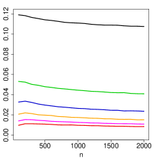
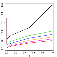
$r_{u_{0},\delta}$, $u_{0}=0.75$
c)	d)

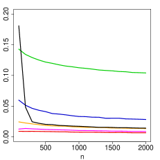
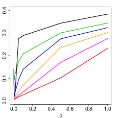
Figure 6: Plot of EMAE, for two choices of the threshold $u_{0}$. Panels a) and c) display the EMAE as a function of the sample size $n$, when $c=0.01$, while panels b) and d) present the EMAE as a function of the penalizing constant $c$ when $n=1000$ (b) and d). In all cases, the errors standard deviation equals $\sigma=0.01$. The black, green, blue, orange, magenta and red lines represent the EMAE for $\delta=1,\,0,\,-\,0.5,\,-\,1,\,-\,1.5$ and $\,-\,2$.

To analyse the behaviour of the EMAE according to the smoothness of the regression function $r_{u_{0},\delta}$ given by the parameter $\delta$, panels a) and c) in Figure 6 present a plot of EMAE as a function of $n$ for four values of $\delta$ when $c=0.01$, while panels b) and d) display the EMAE as a function of the penalizing constant $c$ also for four choices of $\delta$ and $n=1000$. The standard deviation $\sigma$ was set equal to $0.01$ in all cases. When $u_{0}=0.5$, the green, violet, orange and magenta lines represent the EMAE for $\delta=0,\,-\,0.5,\,-\,1$ and $\,-\,1.5$, while for $u_{0}=0.75$, the blue, green, orange and grey lines correspond to $\delta=1,0,,\,-\,1$ and $\,-\,2$. Note that the case $\delta=\,-\,1$ was already considered in the left panels of Figure 5, labelled a) and c), for $\sigma=0.01$ for three sample sizes. The obtained plots illustrate that the empirical mean absolute error is smaller as the absolute value of $\delta$ increases, confirming that the linear relationship is easier to detect as the jump of the derivative of the regression function at the threshold becomes larger.

$r_{u_{0},\delta}$, $u_{0}=0.5$
$\delta=\,-1$	$\delta=\,0$	$\delta=\,1$
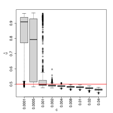
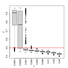
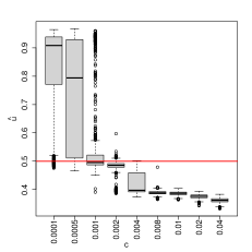
$r_{u_{0},\delta}$, $u_{0}=0.75$
$\delta=\,-1$	$\delta=\,0$	$\delta=\,1$

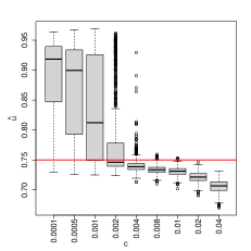
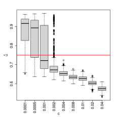
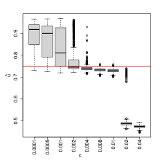
Figure 7: Boxplots of the estimators $\widehat{u}$ for different choices of the penalizing constant $c$, when $n=500$ and $\sigma=0.01$. The horizontal red line corresponds to the true value $u_{0}$.

As an illustration of the finite sample estimators behaviour, Figure 7 displays parallel boxplots of the estimators of the threshold ${u}_{0}$ for different choices of the penalizing constant $c$, when $u_{0}=0.5$ and $0.75$, $\delta=-1,0$ and $1$, $\sigma=0.01$ and the sample size equals 500. Similar plots are obtained for other values of $n$. The true parameter is indicated with the horizontal solid red line. For both choices of $u_{0}$ and the three values of $\delta$, the constant $c$ takes values in $\{0.0001,0.0005,0.001,0.002,0.004,$ $0.008,0.01,0.02,0.04\}$. Figure 7 shows that, as expected, for small values of $c$ values, the threshold estimates are larger than the target. In contrast, large values of $c$ lead to boxplots of $\widehat{u}$ that lie below the true threshold. In all the considered situations, for one of the selected values of $c$, the boxplot of the estimates is centered at ${u}_{0}$. These plots also explain the EMAE results displayed in the left panel of Figure 5. Figures 8 and 9 display the boxplots when $\sigma=0.05$ and $0.10$, for proper grid values of $c$. Similar conclusions arise for these values of the standard deviation, but it should be noticed that, as expected, as expected, larger values of the constant $c$ are desirable as $\sigma$ increases. This behaviour was already observed in Figure 5.

$r_{u_{0},\delta}$, $u_{0}=0.5$
$\delta=\,-1$	$\delta=\,0$	$\delta=\,1$
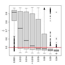
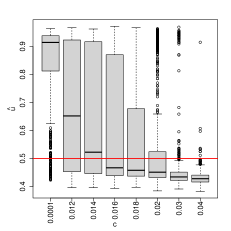
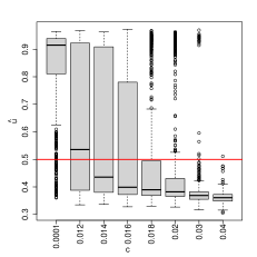
$r_{u_{0},\delta}$, $u_{0}=0.75$
$\delta=\,-1$	$\delta=\,0$	$\delta=\,1$

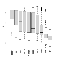
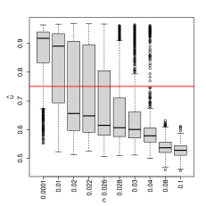
Figure 8: Boxplots of the estimators $\widehat{u}$ for different choices of the penalizing constant $c$, when $n=500$ and $\sigma=0.05$. The horizontal red line corresponds to the true value $u_{0}$.

$r_{u_{0},\delta}$, $u_{0}=0.5$
$\delta=\,-1$	$\delta=\,0$	$\delta=\,1$
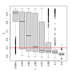
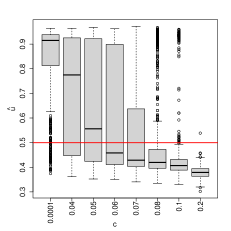
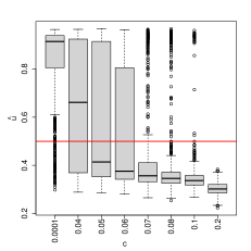
$r_{u_{0},\delta}$, $u_{0}=0.75$
$\delta=\,-1$	$\delta=\,0$	$\delta=\,1$

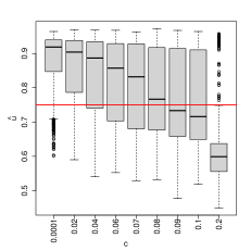
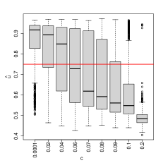
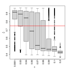
Figure 9: Boxplots of the estimators $\widehat{u}$ for different choices of the penalizing constant $c$, when $n=500$ and $\sigma=0.10$. The horizontal red line corresponds to the true value $u_{0}$.

$r_{u_{0},\delta}$, $u_{0}=0.5$
$\delta=\,-1$	$\delta=\,0$	$\delta=\,1$
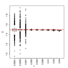
$r_{u_{0},\delta}$, $u_{0}=0.75$
$\delta=\,-1$	$\delta=\,0$	$\delta=\,1$

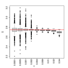
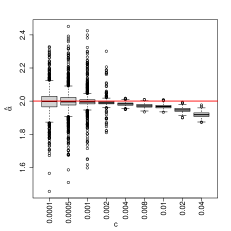
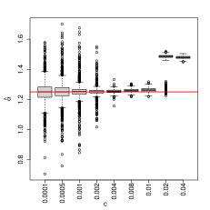
Figure 10: Boxplots of the estimators $\widehat{\alpha}$ for different choices of the penalizing constant $c$, when $n=500$ and $\sigma=0.01$. The horizontal red line corresponds to the value $\alpha_{0}$.

Figures 10 and 11 present the boxplots of the estimators $\widehat{\alpha}_{\widehat{u}}$ and $\widehat{\beta}_{\widehat{u}}$, respectively when $\sigma=0.01$. The boxplots when $\sigma=0.05$ and $0.10$ are displayed in Figures 12 to 15. In each Figure, the horizontal solid red line corresponds to the true parameters $\alpha_{0}$ and $\beta_{0}$, respectively. Taking into account that for values of $c$ smaller than $0.001$, the threshold estimates are mainly larger or equal than the target, the estimates of the slope and intercept accomplish the goal since their boxplots are centered around the true values. On the contrary, for large values of $c$ some of the observations used to estimate the slope and intercept correspond to data generated using the function $g(x)$, that is, with the nonparametric model component and for that reason, they fail in their purpose.

$r_{u_{0},\delta}$, $u_{0}=0.5$
$\delta=\,-1$	$\delta=\,0$	$\delta=\,1$
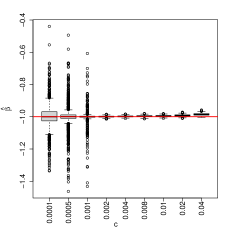
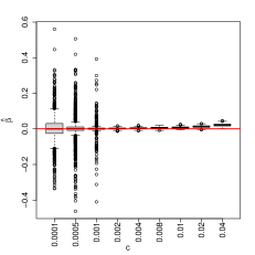
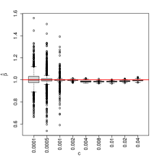
$r_{u_{0},\delta}$, $u_{0}=0.75$
$\delta=\,-1$	$\delta=\,0$	$\delta=\,1$

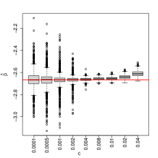
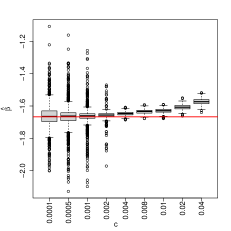
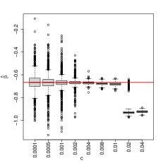
Figure 11: Boxplots of the estimators $\widehat{\beta}$ for different choices of the penalizing constant $c$, when $n=500$ and $\sigma=0.01$. The horizontal red line corresponds to the value $\beta_{0}$.

$r_{u_{0},\delta}$, $u_{0}=0.5$
$\delta=\,-1$	$\delta=\,0$	$\delta=\,1$
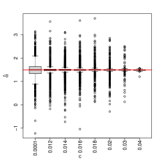
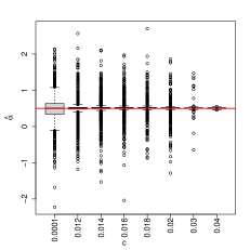
$r_{u_{0},\delta}$, $u_{0}=0.75$
$\delta=\,-1$	$\delta=\,0$	$\delta=\,1$

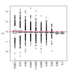
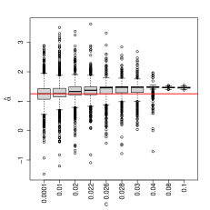
Figure 12: Boxplots of the estimators $\widehat{\alpha}$ for different choices of the penalizing constant $c$, when $n=500$ and $\sigma=0.05$. The horizontal red line corresponds to the value $\alpha_{0}$.

$r_{u_{0},\delta}$, $u_{0}=0.5$
$\delta=\,-1$	$\delta=\,0$	$\delta=\,1$
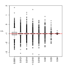
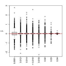
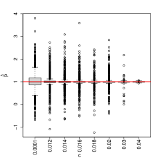
$r_{u_{0},\delta}$, $u_{0}=0.75$
$\delta=\,-1$	$\delta=\,0$	$\delta=\,1$

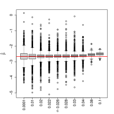
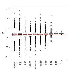
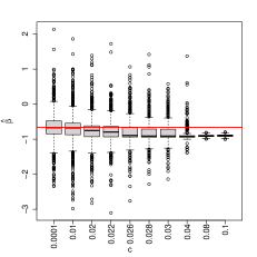
Figure 13: Boxplots of the estimators $\widehat{\beta}$ for different choices of the penalizing constant $c$, when $n=500$ and $\sigma=0.05$. The horizontal red line corresponds to the value $\beta_{0}$.

$r_{u_{0},\delta}$, $u_{0}=0.5$
$\delta=\,-1$	$\delta=\,0$	$\delta=\,1$
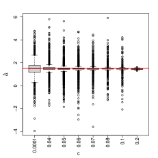
$r_{u_{0},\delta}$, $u_{0}=0.75$
$\delta=\,-1$	$\delta=\,0$	$\delta=\,1$

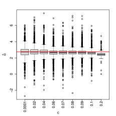
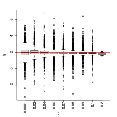
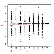
Figure 14: Boxplots of the estimators $\widehat{\alpha}$ for different choices of the penalizing constant $c$, when $n=500$ and $\sigma=0.10$. The horizontal red line corresponds to the value $\alpha_{0}$.

$r_{u_{0},\delta}$, $u_{0}=0.5$
$\delta=\,-1$	$\delta=\,0$	$\delta=\,1$
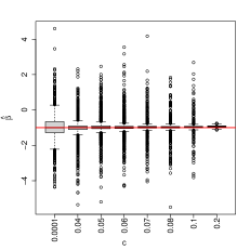
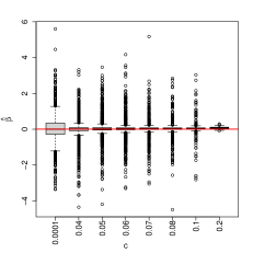
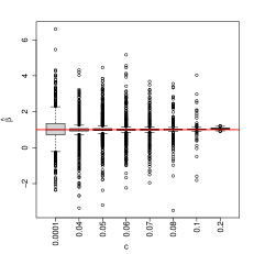
$r_{u_{0},\delta}$, $u_{0}=0.75$
$\delta=\,-1$	$\delta=\,0$	$\delta=\,1$

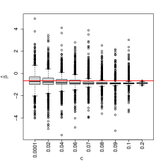
Figure 15: Boxplots of the estimators $\widehat{\beta}$ for different choices of the penalizing constant $c$, when $n=500$ and $\sigma=0.10$. The horizontal red line corresponds to the value $\beta_{0}$.

5 A real data example

In this section, we analyse the airquality real data set studied in Cleveland, (1985). This data set was used therein as a wire conductor to present different graphical tools. As mentioned in the Introduction, the aim of the analysis is to study the relation between the ozone concentration and the wind speed, that is, the response variable $Y$ is the ozone concentration and the predictor $X$ corresponds to the wind speed. As mentioned in the Introduction, we consider the 111 cases studied in Cleveland, (1985) which correspond to the data that do not contain missing observations.

a)	b)	c)

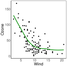
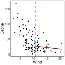
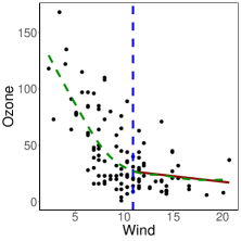
Figure 16: Air quality data (black points) with two different fits: a) lowess fit and b) threshold regression model with $\widehat{u}=10.9$, $\widehat{\alpha}_{\widehat{u}}=37.658$ and $\widehat{\beta}_{\widehat{u}}=\,-\,0.996$. Panel c) displays both fits over imposed.

The left panel in Figure 16 displays the data (in black points) together with a solid green line corresponding to the fit obtained using local polynomials through the function lowess in R, see Cleveland, (1979, 1981). This plot mimics Figure 1.4 of the above mentioned book and as mentioned therein the nonparametric smoother suggests that the linear fit is not appropriate all over the support of the covariates. In this sense, an important point is to find the wind speed from which the model may be assumed to be linear and our approach though threshold regression models becomes useful.

The middle panel in Figure 16 presents the data and the result obtained for the threshold regression model represented with a solid red line. More precisely, we use the threshold estimator introduced in this paper, to get the best wind speed above which the linear model can be used. For that purpose, the possible values of $u$ vary along the observed values of the predictor, up to its $98\%$ empirical quantile that corresponds to $u=18.4$.

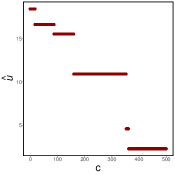
Figure 17: Estimated thresholds (18.4, 16.6, 15.5, 10.9, 4.6 and 2.3) as a function of $c$, using the penalizing term $\lambda_{n}=cn^{-0.4}$ and $f(u)=u$. The cut-off $\gamma_{n}$ is the $98\%-$empirical quantile of the predictors.

Figure 17 displays the obtained values of the estimated threshold according to different values of the constant $c$ included the penalizing term defined as $\lambda_{n}f(u)=c\;n^{-0.4}f(u)$, where as in the simulation study $f(u)=u$ for $u\geq 0$ and $f(u)=0$ for $u\leq 0$. The values of $c$ were chosen in the interval $[0,500]$, using an grid with different grid steps, to be more precise, in the interval $[0,10]$ the increment between consecutive points was $0.001$, between 10.01 and 150 it was 0.01, while in the interval $[150.1,500]$ the spacing was $0.1$. Figure 17 reveals that the threshold is a step function of $c$ leading to six possible thresholds which were obtained as $c$ varies along the considered interval. As expected, for $c$ too small, we can not prevent an overfit phenomenon which leads to estimated thresholds equal to $\widehat{u}=18.4$, $16.6$ and $15.5$ meaning that in almost all the support the model is considered nonparametric. In contrast, for very large values of $c$ the penalization term dominates the objective function, estimating the threshold as the left extreme of the interval ($\widehat{u}=2.3$), suggesting that the linear regression could be used in the entire domain of the predictor. Interestingly, $\widehat{u}=10.9$ is observed for an intermediate regime, indicating that 10.9 may be a possible value above which the linear model may be used. The fit displayed in the middle panel of Figure 16 corresponds to this last value. Panel c) in Figure 16 displays the local smoother in dashed green lines together with the linear fit above the estimated threshold plotted as a solid red line. The plot suggests that the considered linear fit is appropriate for values of the wind speed larger or equal than 10.9.

Taking into account the asymptotic behaviour provided in Theorem 3.3 for the intercept and slope estimators, when considering values larger than the estimated threshold, we chose $\psi=1$ and we performed a linear fit for those observations above $\widehat{u}+\psi=11.9$ obtaining $\widehat{\alpha}_{\widehat{u}+\psi}=42.096$ and $\widehat{\beta}_{\widehat{u}+\psi}=\,-\,1.280$. For this cut–off value, the slope estimator $\widehat{\beta}_{\widehat{u}+\psi}$ is not significantly different from 0 suggesting that for large values of the wind speed the ozone remains constant.

6 Final comments

In this paper, we introduce a new model, called threshold regression semiparametric model, that attempts to overcome the limitations presented by the linear model while maintaining its simplicity and interpretability. The considered model tries to keep the validity of the linear model in the biggest possible domain for large values of the covariate, while no shape assumptions on the regression function are assumed for values smaller than the threshold. This is an advantage over segmented linear regression or the so–called bent linear regression with an unknown change point, since the threshold regression semiparametric model does not require that the regression function is also linear before the change point.

A procedure to consistently estimate the threshold as well as the intercept and slope of the linear component of the regression function is introduced. The numerical results reflects that, as expected, the non–penalized threshold estimates do not converge to the true threshold and confirms the consistency results derived in Theorem 3.1 when a penalty term converging at a rate smaller than root-$n$ is included. Furthermore, the obtained results reflect that the rate of convergence may depend on the regression smoothness. The benefits of our model are illustrated over the air quality data set providing simple but flexible model. The threshold model allows to understand the relation between the ozone concentration and the wind speed for high values of the speed through a simple linear regression model.

An important topic to be mentioned is that our approach allows for more general semiparametric models, where non-parametric and parametric regimes are allowed under a unified framework. For instance, the model and the estimation method introduced may be easily extended to other parametric models beyond the simple linear regression postulated for the regression function beyond the threshold. Extensions to a threshold generalized linear model are also an important issue which is beyond the scope of the paper and will be object of future work.

As is well known, estimators based on least squares are usually affected by atypical data, that is, by observations with large residuals in particular if combined with covariates with high leverage. In this sense, robust procedures may be important to mitigate the impact of outliers in the estimation process, both for linear or more general parametric regression models beyond a threshold. The result provided in Proposition 3.1 suggests that other loss functions instead of the squared loss may be used to define resistant and consistent estimators. This interesting topic is now part of ongoing research.

A Appendix: Proofs

A.1 Proof of Lemma 2.1

In the sequel, to alleviate the notation, we will use the sub index $u$ to operate conditioned on $\{X\geq u\}$. For instance, $\mathbb{E}_{u}(W)$, $\mathbb{V}ar_{u}(X)$ and $\mathbb{C}ov_{u}(X,Y)$ stand for $\mathbb{E}(W\mid X\geq u)$, $\mathbb{E}(X^{2}\mid X\geq u)-\mathbb{E}^{2}(X\mid X\geq u)$ and $\mathbb{E}(XY\mid X\geq u)-\mathbb{E}(X\mid X\geq u)\mathbb{E}(Y\mid X\geq u)$, respectively. As mentioned above, if $u=-\infty$ no restrictions are made when conditioning.

Proof of Lemma 2.1.

Recall that, for $u<b$, $(\alpha_{u},\beta_{u})$ are the best coefficient for linearly approximate $Y$ based on $X$ when $X\geq u$, that is, they are defined through (3). Therefore, we have that

$$\beta_{u}=\frac{\mathbb{C}ov_{u}(X,Y)}{\mathbb{V}ar_{u}(X)}\qquad\mbox{and}\qquad\alpha_{u}=\mathbb{E}_{u}(Y)-\beta_{u}\mathbb{E}_{u}(X)\,.$$

Note that, as mentioned in Section 2.1, when $u_{0}\neq-\infty$, for any $u\geq u_{0}$, we have that $(\alpha_{u},\beta_{u})=(\alpha_{0},\beta_{0})$, while in the case, when $u_{0}=-\infty$, $(\alpha_{0},\beta_{0})=(\alpha_{u},\beta_{u})$ for any $u<b$.

a) Using that from C2, the marginal distribution function of $X$ is continuous, from the Lebesgue Dominated Convergence Theorem we obtain that $\alpha_{u}$ and $\beta_{u}$ depend continuously on $u$ and that $\ell(\cdot)$ is also a continuous function on $(-\infty,b)$.

b) Using that $Y=r(X)+\varepsilon$, the independence between the errors and the covariates and that $\mathbb{E}(\varepsilon)=0$ from C1, we obtain that $\ell(u)$ can be written as

$$\ell(u)=\mathbb{E}_{u}\left[\left\{Y-(\alpha_{u}+\beta_{u}X)\right\}^{2}\right]=\mathbb{E}_{u}\left[\left\{r(X)-(\alpha_{u}+\beta_{u}X)\right\}^{2}\right]+\mathbb{E}\left(\varepsilon^{2}\right)\,.$$ (A.1)

On the one hand, when $u_{0}\neq-\infty$, the desired result follows from the facts that $\mathbb{P}(r(X)=\alpha_{0}+\beta_{0}\,X\mid X\geq u)=1$ and $(\alpha_{0},\beta_{0})=(\alpha_{u},\beta_{u})$, for any $u\geq u_{0}$. On the other hand, when $u_{0}=-\infty$, we have that $\mathbb{P}(r(X)=\alpha_{0}+\beta_{0}\,X)=1$ and $(\alpha_{0},\beta_{0})=(\alpha_{u},\beta_{u})$, for any $u<b$, which concludes the proof of b).

c) Let us consider the situation where $a<u<u_{0}$ and assume that $\ell(u)=\ell(u_{0})$. Using (A.1), we conclude that $\mathbb{E}_{u}[\{r(X)-(\alpha_{u}+\beta_{u}X)\}^{2}]=0$ which leads to $\mathbb{P}\left(r(X)=\alpha_{u}+\beta_{u}X\mid X\geq u\right)=1$ contradicting the definition of $u_{0}$.

On the other hand, if $a\neq-\infty$ and $u\leq a$, we get that we get that $\alpha_{u}=\alpha_{a}$ and $\beta_{u}=\beta_{a}$, so

$$\ell(u)=\mathbb{E}\left[\left\{r(X)-(\alpha_{a}+\beta_{a}X)\right\}^{2}\right]+\mathbb{E}\left(\varepsilon^{2}\right)=\ell(a)\,,$$ (A.2)

which is bigger than $\ell(u_{0})=\mathbb{E}(\varepsilon^{2})$, by C4. Hence, $\ell(u)>\ell(u_{0})$ for any $u<u_{0}$, concluding the proof.

d) We need to show that

$$A_{\delta}=\inf_{\{u\leq u_{0}-\delta\}}\ell(u)>\ell(u_{0})\;.$$

To do so, let $\{u_{k}\}_{k\in\mathbb{N}}$ be a sequence such that $u_{k}\leq u_{0}-\delta$ and $\lim_{k\to\infty}\ell(u_{k})=A_{\delta}$. If the sequence $\{u_{k}\}_{k\in\mathbb{N}}$ is bounded, there exists a convergent subsequence $\{u_{k_{j}}\}_{j\in\mathbb{N}}$. Let $u^{\star}$ be such that $\lim_{j\to\infty}u_{k_{j}}=u^{\star}$, then $u^{\star}\leq u_{0}-\delta$ and the continuity of the function $\ell$ implies that $A_{\delta}=\lim_{j\to\infty}\ell(u_{k_{j}})=\ell(u^{\star})$, so using c) we obtain that $\ell(u^{\star})>\ell(u_{0})$, concluding the proof.

If $a\neq\,-\,\infty$, the approximating sequence $\{u_{k}\}_{k\in\mathbb{N}}$ may always be assumed to be bounded below since $\ell$ is constant for $u\leq a$. In that case the proof is completed.

If $a=\,-\,\infty$ and the sequence $\{u_{k}\}_{k\in\mathbb{N}}$ is not bounded below, there exists a subsequence $\{u_{k_{j}}\}_{j\in\mathbb{N}}$ such that $\lim_{j\to\infty}u_{k_{j}}=\,-\,\infty$. Denote

$$\beta^{*}=\frac{\mathbb{C}ov(X,Y)}{\mathbb{V}ar(X)}\qquad\mbox{and}\qquad\alpha^{*}=\mathbb{E}(Y)-\beta^{*}\mathbb{E}(X)\,.$$ (A.3)

Arguing as in b), we obtain that

$$A_{\delta} =\lim_{j\to\infty}\ell(u_{k_{j}})=\mathbb{E}\left\{Y-\left(\alpha^{*}+\beta^{*}X\right)\right\}^{2}$$

$$=\mathbb{E}\left\{r(X)-\left(\alpha^{*}+\beta^{*}X\right)\right\}^{2}+\mathbb{E}\left(\varepsilon^{2}\right)>\ell(u_{0})\,,$$ (A.4)

where the last inequality follows from C4, since $\mathbb{P}\left(r(X)=\alpha^{*}+\beta^{*}X\right)<1$. ∎

A.2 Proof of Proposition 3.1

In this section, we include the proof of Proposition 3.1 which is a general result allowing to derive Theorem 3.1.

Proof of Proposition 3.1.

Take $\widetilde{\gamma}>\gamma$, such that $1-F_{X}(\widetilde{\gamma})>0$ and define

$$W_{n}=\sup_{u\leq u_{0}}|\widehat{\ell}(u,{\mathcal{Z}}_{n})-\ell(u)|\quad\text{ and }\quad T_{n}=\sup_{u\in[u_{0},\widetilde{\gamma}]}|\widehat{\ell}(u,{\mathcal{Z}}_{n})-\ell(u)|\,.$$

Using that $\gamma_{n}\buildrel a.s.\over{\longrightarrow}\gamma$, we have that there exists a null probability set $\mathcal{N}$ such that $\gamma_{n}\to\gamma$, for any $\omega\notin\mathcal{N}$. Denote $\delta_{0}=(\gamma-u_{0})/2$, $\delta_{0}^{\star}=(\widetilde{\gamma}-\gamma)/2$ and $\delta_{1}=\min(\delta_{0},\delta_{0}^{\star})$. Then, we have that $u_{0}+\delta_{1}<u_{0}+\delta_{0}=\gamma-\delta_{0}$ and $\gamma+\delta_{1}<\gamma+\delta_{0}^{\star}=\widetilde{\gamma}$, so

$$\lim_{n\to\infty}\mathbb{P}(\mathcal{A}_{n})=\mathbb{P}(u_{0}+\delta_{1}<\gamma_{n}<\widetilde{\gamma})=1\,,$$ (A.5)

implying that for any $\omega\in\mathcal{A}_{n}$, we have $u_{0}+\delta<\gamma_{n}<\widetilde{\gamma}$, for any $0<\delta<\delta_{1}$.

From C6, there exists $\delta_{2}>0$ such that $f$ is strictly increasing in $[u_{0}-\delta_{2},u_{0}+\delta_{2}]$. We will show that for any $0<\delta<\min(\delta_{1},\delta_{2})$ there exists $\nu>0$ such that

$$\{W_{n}\leq\nu\}\;\subseteq\;\left\{\mathrm{PL}(u_{0},{\mathcal{Z}}_{n})<\mathrm{PL}(u,{\mathcal{Z}}_{n})\>,\quad\hbox{for $u<u_{0}-\delta$}\right\}$$ (A.6)

and that, for $n$ large enough, we have that

$$\mathcal{A}_{n}\cap\{T_{n}\leq a_{n}\}\subseteq\;\left\{\mathrm{PL}(u_{0},{\mathcal{Z}}_{n})<\mathrm{PL}(u,{\mathcal{Z}}_{n})\>,\quad\hbox{for $u_{0}+\delta<u<\widetilde{\gamma}$}\right\}\;.$$ (A.7)

Note that from (A.6) and (A.7) using that $\widehat{u}_{n}<\gamma_{n}$ , we obtain that

$$\mathcal{A}_{n}\,\cap\,\{W_{n}\leq\nu\}\,\cap\,\{T_{n}\leq a_{n}\}\;\subseteq\;\left\{\,|\widehat{u}_{n}-u_{0}|\leq\delta\,\right\}\,,$$

which, together with (A.5) and the convergences assumed in (a) and (b), entail that $\mathbb{P}\left(|\widehat{u}_{n}-u_{0}|\leq\delta\right)\to 1$ as $n\to\infty$. Then, if we prove (A.6) and (A.7) we obtain the desired result.

Let us begin by showing that (A.7) holds. Taking into account that $\ell$ satisfies (5), we have that $\ell(u)=\ell(u_{0})$, for any $u_{0}\leq u\leq\widetilde{\gamma}$, therefore we obtain that

$$\mathrm{PL}(u,{\mathcal{Z}}_{n})-\mathrm{PL}(u_{0},{\mathcal{Z}}_{n}) \;=\;\widehat{\ell}(u,{\mathcal{Z}}_{n})-\widehat{\ell}(u_{0},{\mathcal{Z}}_{n})+\lambda_{n}(f(u)-f(u_{0}))$$

$$\;=\;\widehat{\ell}(u,{\mathcal{Z}}_{n})-\ell(u)+\ell(u_{0})-\widehat{\ell}(u_{0},{\mathcal{Z}}_{n})+\lambda_{n}(f(u)-f(u_{0}))$$

$$\;\geq\;-2a_{n}+\lambda_{n}(f(u)-f(u_{0}))\,,$$

where the last inequality follows from the fact that $T_{n}\leq a_{n}$. Note that C6 implies that $f(u)\geq f(u_{0}+\delta)$, for any $u>u_{0}+\delta$. Furthermore, using that $\delta<\delta_{2}$, we get that $f(u_{0}+\delta)-f(u_{0})>0$. Then, using that $\mathcal{A}_{n}\subset\{u_{0}+\delta<\gamma_{n}<\widetilde{\gamma}\}$, we get that on $\mathcal{A}_{n}\cap\{T_{n}\leq a_{n}\}$, for any $u_{0}+\delta<u<\widetilde{\gamma}$, we have that

$$\mathrm{PL}(u,{\mathcal{Z}}_{n})-\mathrm{PL}(u_{0},{\mathcal{Z}}_{n}) \geq\lambda_{n}\left\{(f(u_{0}+\delta)-f(u_{0}))-2\frac{a_{n}}{\lambda_{n}}\right\}>0\,,$$

for $n$ large enough, since $a_{n}/\lambda_{n}\to 0$ as $n\to\infty$.

It remains to prove that (A.6) holds. Note that since $\ell$ satisfies (7), we have that

$$\inf_{u\leq u_{0}-\delta}\ell(u)-\ell(u_{0})=\nu_{\delta}>0\,.$$ (A.8)

Choosing $\nu=\nu_{\delta}/4$ and using that $f$ is a non-negative function, we obtain that, for any $u<u_{0}-\delta$, if $W_{n}\leq\nu$ then

$$\mathrm{PL}(u,{\mathcal{Z}}_{n})-\mathrm{PL}(u_{0},{\mathcal{Z}}_{n}) \;=\;\widehat{\ell}(u,{\mathcal{Z}}_{n})-\widehat{\ell}(u_{0},{\mathcal{Z}}_{n})+\lambda_{n}(f(u)-f(u_{0}))$$

$$\;=\;\widehat{\ell}(u,{\mathcal{Z}}_{n})-\ell(u)+\ell(u_{0})-\widehat{\ell}(u_{0},{\mathcal{Z}}_{n})+\ell(u)-\ell(u_{0})$$

$$\hskip 28.90755pt+\lambda_{n}(f(u)-f(u_{0}))$$

$$\;\geq\;-2W_{n}+\ell(u)-\ell(u_{0})-\lambda_{n}f(u_{0})$$

$$\;\geq\;-2\alpha+\nu_{\delta}-\lambda_{n}f(u_{0})=\frac{\nu_{\delta}}{2}-\lambda_{n}f(u_{0})>0$$

for $n$ large enough, since $\lambda_{n}\to 0$. ∎

A.3 Some preliminary results

In this section, we include two results which are a key step to derive Theorem 3.1 from Proposition 3.1. They will also be useful to prove Corollary 3.2 and Theorem 3.3. Their proof use standard empirical processes tools.

In the sequel, we adopt the following notation that strengths the dependence on the regression coefficients

$$\widehat{\ell}(u,\alpha,\beta) =\frac{\mathbb{P}_{n}\left[\{Y-(\alpha+\beta X)\}^{2}\mathbb{I}_{\{X\geq u\}}\right]}{\mathbb{P}_{n}\left(\mathbb{I}_{\{X\geq u\}}\right)}\;,$$

$$\ell(u,\alpha,\beta) =\frac{\mathbb{P}\left[\{Y-(\alpha+\beta X)\}^{2}\mathbb{I}_{\{X\geq u\}}\right]}{\mathbb{P}\left(\mathbb{I}_{\{X\geq u\}}\right)}\,.$$

In this way, we get that $\widehat{\ell}(u,{\mathcal{Z}}_{n})=\widehat{\ell}(u,\widehat{\alpha}_{u},\widehat{\beta}_{u})$ and $\ell(u)=\ell(u,\alpha_{u},\beta_{u})$.

The proof of Lemma A.2 needs also a basic result stated below.

Lemma A.1.

Let $\{(X_{i},Y_{i}):i\geq 1\}$ are i.i.d., distributed as $(X,Y)$ and fix $s,m\in\mathbb{N}$. Then, if $\mathbb{E}(X^{2s}\,Y^{2m})<\infty$, we have that the class of functions ${\mathcal{H}}=\{h(x,y)=x^{s}y^{m}\mathbb{I}_{\{x\geq u\}},\;u\in\mathbb{R}\}$ is $P-$Donsker, , where $P$ stands for the joint probability measure of $(X,Y)$, so

$$\sqrt{n}\displaystyle\sup_{u\in\mathbb{R}}\left|\,\mathbb{P}_{n}\left(X^{s}Y^{m}\mathbb{I}_{\{X\geq u\}}\right)-\mathbb{P}\left(X^{s}Y^{m}\mathbb{I}_{\{X\geq u\}}\right)\,\right|=O_{\mathbb{P}}(1)\;.$$ (A.9)

Proof.

Lemma 2.6.15 in van der Vaart and Wellner, (1996) implies that the class of functions $\mathcal{G}=\{g(x,y)=x-u,\;u\in\mathbb{R}\}$ is a VC-subgraph class of functions with VC-index smaller or equal that 3. Then, from Lemmas 9.8 and 9.9 (iii) in Kosorok, (2008), we conclude that $\mathcal{G}^{\star}=\{g(x,y)=\mathbb{I}_{\{x\geq u\}},\;u\in\mathbb{R}\}$ is also a VC-subgraph class of functions. Using the permanence properties of VC-classes stated in Lemma 9.9 (iv) from Kosorok, (2008), we obtain that ${\mathcal{H}}$ is also a VC-subgraph class of functions. Note that ${\mathcal{H}}$ has envelope $H(X,Y)=|X|^{s}|Y|^{m}$ which belongs to $L^{2}(P)$, since we assumed that $\mathbb{E}(X^{2s}\,Y^{2m})<\infty$. Thus, from Lemma 2.6.7 in van der Vaart and Wellner, (1996), we get that $\mathcal{H}$ satisfies the uniform entropy bound, which together with Theorem 2.5.2 in van der Vaart and Wellner, (1996) implies that $\mathcal{H}$ is a $P-$Donsker’s class, concluding the proof of (A.9). ∎

Lemma A.2.

Assume $\{(X_{i},Y_{i}):i\geq 1\}$ are i.i.d., distributed as $(X,Y)$ satisfying the regression model (1) and let $u_{0}$ be defined as in (2).. Assume that C1, C2 and C4 to C7 hold. Let $\widehat{u}_{n}$ be defined as in (11) and $\widehat{\ell}(u,{\mathcal{Z}}_{n})$ defined in (9). Then, for any fixed $\widetilde{\gamma}=F_{X}^{-1}(1-\eta)$ with $\eta>0$, we have that

1. $\sup_{u\leq\widetilde{\gamma}}\sqrt{n}(\widehat{\alpha}_{u}-\alpha_{u})=O_{\mathbb{P}}(1)\;\quad\hbox{and}\quad\sup_{u\leq\widetilde{\gamma}}\sqrt{n}(\widehat{\beta}_{u}-\beta_{u})=O_{\mathbb{P}}(1)$.

2. $\sup_{u\leq\widetilde{\gamma}}\sqrt{n}|\widehat{\ell}(u,\widehat{\alpha}_{u},\widehat{\beta}_{u})-\widehat{\ell}(u,\alpha_{u},\beta_{u})|=O_{\mathbb{P}}(1)$.

3. $\sup_{u\leq\widetilde{\gamma}}\sqrt{n}|\widehat{\ell}(u,\alpha_{u},\beta_{u})-\ell(u,\alpha_{u},\beta_{u})|=O_{\mathbb{P}}(1)$.

It is worth mentioning that when the support of ${\mathcal{S}}=[a,b]$ is bounded below, that is, when $a\neq-\infty$, the supremum over $u\leq\widetilde{\gamma}$ equals that computed over $a\leq u\leq\widetilde{\gamma}$, since for values of $u$ smaller than $a$, $\mathbb{I}_{\{X\geq u\}}=1$. For that reason, in the proof below we consider the limits when $u\to a$ instead of $u\to-\infty$. The case of unbounded supports is included having in mind that in such situation $a=-\infty$.

Proof of Lemma A.2.

To prove (a) note that

$$\sqrt{n}\,(\widehat{\alpha}_{u}-\alpha_{u})=A_{1,n}(u)-\beta_{u}\,A_{2,n}(u)-\sqrt{n}\,\left(\widehat{\beta}_{u}-\beta_{u}\right)\frac{\mathbb{P}_{n}\left(Y\mathbb{I}_{\{X\geq u\}}\right)}{\mathbb{P}_{n}\left(\mathbb{I}_{\{X\geq u\}}\right)}\,,$$

where

$$A_{1,n}(u) =\sqrt{n}\,\left\{\frac{\mathbb{P}_{n}\left(Y\mathbb{I}_{\{X\geq u\}}\right)}{\mathbb{P}_{n}\left(\mathbb{I}_{\{X\geq u\}}\right)}-\frac{\mathbb{P}\left(Y\mathbb{I}_{\{X\geq u\}}\right)}{\mathbb{P}\left(\mathbb{I}_{\{X\geq u\}}\right)}\right\}$$

$$=\frac{\sqrt{n}\left\{\mathbb{P}_{n}\left(Y\mathbb{I}_{\{X\geq u\}}\right)-\mathbb{P}\left(Y\mathbb{I}_{\{X\geq u\}}\right)\right\}\,\mathbb{P}\left(\mathbb{I}_{\{X\geq u\}}\right)-\mathbb{P}\left(Y\mathbb{I}_{\{X\geq u\}}\right)\,\sqrt{n}\left\{\mathbb{P}_{n}\left(\mathbb{I}_{\{X\geq u\}}\right)-\mathbb{P}\left(\mathbb{I}_{\{X\geq u\}}\right)\right\}}{\mathbb{P}\left(\mathbb{I}_{\{X\geq u\}}\right)\mathbb{P}_{n}\left(\mathbb{I}_{\{X\geq u\}}\right)}\,,$$

$$A_{2,n}(u) =\sqrt{n}\,\left\{\frac{\mathbb{P}_{n}\left(X\mathbb{I}_{\{X\geq u\}}\right)}{\mathbb{P}_{n}\left(\mathbb{I}_{\{X\geq u\}}\right)}-\frac{\mathbb{P}\left(X\mathbb{I}_{\{X\geq u\}}\right)}{\mathbb{P}\left(\mathbb{I}_{\{X\geq u\}}\right)}\right\}$$

$$=\frac{\sqrt{n}\left\{\mathbb{P}_{n}\left(X\mathbb{I}_{\{X\geq u\}}\right)-\mathbb{P}\left(X\mathbb{I}_{\{X\geq u\}}\right)\right\}\,\mathbb{P}\left(\mathbb{I}_{\{X\geq u\}}\right)-\mathbb{P}\left(X\mathbb{I}_{\{X\geq u\}}\right)\,\sqrt{n}\left\{\mathbb{P}_{n}\left(\mathbb{I}_{\{X\geq u\}}\right)-\mathbb{P}\left(\mathbb{I}_{\{X\geq u\}}\right)\right\}}{\mathbb{P}\left(\mathbb{I}_{\{X\geq u\}}\right)\mathbb{P}_{n}\left(\mathbb{I}_{\{X\geq u\}}\right)}\,.$$

Therefore, noticing that from Lemma A.1,

$$\sqrt{n}\sup_{u\leq\widetilde{\gamma}}\left|\mathbb{P}_{n}\left(Y\mathbb{I}_{\{X\geq u\}}\right)-\mathbb{P}\left(Y\mathbb{I}_{\{X\geq u\}}\right)\right| =O_{\mathbb{P}}(1)\,,$$

$$\sqrt{n}\sup_{u\leq\widetilde{\gamma}}\left|\mathbb{P}_{n}\left(X\mathbb{I}_{\{X\geq u\}}\right)-\mathbb{P}\left(X\mathbb{I}_{\{X\geq u\}}\right)\right| =O_{\mathbb{P}}(1)\,,$$

$$\sqrt{n}\sup_{u\leq\widetilde{\gamma}}\left|\mathbb{P}_{n}\left(\mathbb{I}_{\{X\geq u\}}\right)-\mathbb{P}\left(\mathbb{I}_{\{X\geq u\}}\right)\right| =O_{\mathbb{P}}(1)\,,$$

since $\mathbb{E}(X^{2})<\infty$ and $\mathbb{E}(Y^{2})<\infty$, to show that $\sup_{u\leq\widetilde{\gamma}}\sqrt{n}(\widehat{\alpha}_{u}-\alpha_{u})=O_{\mathbb{P}}(1)$ it will be enough to show that $\sup_{u\leq\widetilde{\gamma}}\sqrt{n}(\widehat{\beta}_{u}-\beta_{u})=O_{\mathbb{P}}(1)$.

For that purpose, notice that

$$\beta_{u}\;=\;\frac{\mathbb{P}\left(X\,Y\,\mathbb{I}_{\{X\geq u\}}\right)\;\mathbb{P}\left(\mathbb{I}_{\{X\geq u\}}\right)-\mathbb{P}\left(X\,\mathbb{I}_{\{X\geq u\}}\right)\;\mathbb{P}\left(Y\,\mathbb{I}_{\{X\geq u\}}\right)}{\mathbb{P}\left(X^{2}\,\mathbb{I}_{\{X\geq u\}}\right)\;\mathbb{P}\left(\mathbb{I}_{\{X\geq u\}}\right)-\left\{\mathbb{P}\left(X\,\mathbb{I}_{\{X\geq u\}}\right)\right\}^{2}}=\frac{A(u)}{D(u)}\,,$$

and

$$\widehat{\beta}_{u}\;=\;\frac{\mathbb{P}_{n}\left(X\,Y\,\mathbb{I}_{\{X\geq u\}}\right)\;\mathbb{P}_{n}\left(\mathbb{I}_{\{X\geq u\}}\right)-\mathbb{P}_{n}\left(X\,\mathbb{I}_{\{X\geq u\}}\right)\;\mathbb{P}_{n}\left(Y\,\mathbb{I}_{\{X\geq u\}}\right)}{\mathbb{P}_{n}\left(X^{2}\,\mathbb{I}_{\{X\geq u\}}\right)\;\mathbb{P}_{n}\left(\mathbb{I}_{\{X\geq u\}}\right)-\left\{\mathbb{P}_{n}\left(X\,\mathbb{I}_{\{X\geq u\}}\right)\right\}^{2}}=\frac{A_{n}(u)}{D_{n}(u)}\,.$$

Hence,

$$\sqrt{n}(\widehat{\beta}_{u}-\beta_{u}) =\frac{1}{D_{n}(u)\,D(u)}\;\sqrt{n}\left\{A_{n}(u)D(u)-A(u)D_{n}(u)\right\}$$

$$=\frac{1}{D_{n}(u)\,D(u)}\left\{D(u)\,\sqrt{n}\left(A_{n}(u)-A(u)\right)-A(u)\,\sqrt{n}\left(D_{n}(u)-D(u)\right)\right\}$$ (A.10)

First of all, observe that $\mathbb{V}ar_{u}(X)$ is a continuous function of $u$ which converges to $\mathbb{V}ar(X)$ when $u\to a$, hence $\inf_{u\leq\widetilde{\gamma}}\mathbb{V}ar_{u}(X)>0$. Thus, for all $u\leq\widetilde{\gamma}$ we have that

$$D(u)=\mathbb{P}\left(X^{2}\mathbb{I}_{\{X\geq u\}}\right)\mathbb{P}\left(\mathbb{I}_{\{X\geq u\}}\right)-\left\{\mathbb{P}\left(X\mathbb{I}_{\{X\geq u\}}\right)\right\}^{2}\; =\;\left\{\mathbb{P}\left(X\geq u\right)\right\}^{2}\;\mathbb{V}ar_{u}(X)$$

$$\geq\;\left[1-F_{X}(\widetilde{\gamma})\right]^{2}\inf_{u\leq\widetilde{\gamma}}\mathbb{V}ar_{u}(X)>\;0\;,$$

since $1-F_{X}(\widetilde{\gamma})=\eta>0$, meaning that $D=\inf_{u\leq\widetilde{\gamma}}D(u)>\;0$.

Lemma A.1 entails that $\sup_{u\leq\widetilde{\gamma}}|D_{n}(u)-D(u)|\buildrel p\over{\longrightarrow}0$, so $\lim_{n\to\infty}\mathbb{P}\left(\inf_{u\leq\widetilde{\gamma}}D_{n}(u)>D/2\right)=1$. Thus, taking into account that $\sup_{u\leq\widetilde{\gamma}}D(u)\leq\mathbb{E}(X^{2})$ and $\sup_{u\leq\widetilde{\gamma}}|A(u)|\leq\mathbb{E}|X\,Y|+\mathbb{E}|X|\,\mathbb{E}|Y|<\infty$, from (A.10) we conclude that to show that $\sqrt{n}(\widehat{\beta}_{u}-\beta_{u})=O_{\mathbb{P}}(1)$, it will be enough to prove that

$$\sqrt{n}\left(A_{n}(u)-A(u)\right)=O_{\mathbb{P}}(1)\qquad\mbox{and}\qquad\sqrt{n}\left(D_{n}(u)-D(u)\right)=O_{\mathbb{P}}(1)\,,$$

which follow easily from Lemma A.1, since $\mathbb{E}(X^{2}Y^{2})<\infty$, $\mathbb{E}(X^{2})<\infty$, $\mathbb{E}(Y^{2})<\infty$, see equation (A.9).

b) To prove (b), observe that

$$\widehat{\ell}(u,\alpha_{u},\beta_{u})-\widehat{\ell}(u,\widehat{\alpha}_{u},\widehat{\beta}_{u})\;=\;\frac{\mathbb{P}_{n}\left(\widehat{\Delta}(u)\,\mathbb{I}_{\{X\geq u\}}\right)}{\mathbb{P}_{n}\left(\mathbb{I}_{\{X\geq u\}}\right)}\,,$$ (A.11)

where

$$\widehat{\Delta}(u)=\Big{\{}Y-(\alpha_{u}+\beta_{u}X)\Big{\}}^{2}-\left\{Y-(\widehat{\alpha}_{u}+\widehat{\beta}_{u}X)\right\}^{2}\,.$$

Straightforward calculations allow to see that

$$\widehat{\Delta}(u)=\left(\alpha^{2}_{u}-\widehat{\alpha}^{2}_{u}\right)+\left(\beta^{2}_{u}-\widehat{\beta}^{2}_{u}\right)\,X^{2}-2\left(\alpha_{u}-\widehat{\alpha}_{u}\right)\,Y\,-\,2\,\left(\beta_{u}-\widehat{\beta}_{u}\right)YX\,+\,2\left(\alpha_{u}\beta_{u}-\widehat{\alpha}_{u}\widehat{\beta}_{u}\right)\,X\,.$$

Then, replacing in (A.11) we obtain that

$$\widehat{\ell}(u,\alpha_{u},\beta_{u}) -\widehat{\ell}(u,\widehat{\alpha}_{u},\widehat{\beta}_{u})\;=\;\frac{1}{\mathbb{P}_{n}\left(\mathbb{I}_{\{X\geq u\}}\right)}\Bigl{[}\left(\beta^{2}_{u}-\widehat{\beta}^{2}_{u}\right)\,\mathbb{P}_{n}\left(X^{2}\mathbb{I}_{\{X\geq u\}}\right)-2\left(\alpha_{u}-\widehat{\alpha}_{u}\right)\mathbb{P}_{n}\left(Y\mathbb{I}_{\{X\geq u\}}\right)$$

$$-\,2\,\left(\beta_{u}-\widehat{\beta}_{u}\right)\mathbb{P}_{n}\left(Y\,X\,\mathbb{I}_{\{X\geq u\}}\right)\,+\,2\left(\alpha_{u}\beta_{u}-\widehat{\alpha}_{u}\widehat{\beta}_{u}\right)\mathbb{P}_{n}\left(X\mathbb{I}_{\{X\geq u\}}\right)\Bigr{]}+\left(\alpha^{2}_{u}-\widehat{\alpha}^{2}_{u}\right)\,.$$

Combining the results established in (a), Lemma A.1 and the lower bound for $\mathbb{P}(X\geq u)$ when $u\leq\widetilde{\gamma}$ given by $\mathbb{P}(X\geq u)\geq\eta>0$, the desired result is obtained.

c) Finally, to prove (c) note that

$$\widehat{\ell}(u,\alpha_{u},\beta_{u}) =\frac{\mathbb{P}_{n}\left(\left[Y^{2}-2Y\alpha_{u}\,-\,2\,Y\,X\,\beta_{u}+\,\alpha_{u}^{2}\,+\,\beta_{u}^{2}\,X^{2}\,+\,2\,\alpha_{u}\beta_{u}X\right]\mathbb{I}_{\{X\geq u\}}\right)}{\mathbb{P}_{n}\left(\mathbb{I}_{\{X\geq u\}}\right)}=\frac{B_{n}(u)}{D_{n}(u)}\,,$$

while

$$\ell(u,\alpha_{u},\beta_{u}) =\frac{\mathbb{P}\left(\left[Y^{2}-2Y\alpha_{u}\,-\,2\,Y\,X\,\beta_{u}+\,\alpha_{u}^{2}\,+\,\beta_{u}^{2}\,X^{2}\,+\,2\,\alpha_{u}\beta_{u}X\right]\mathbb{I}_{\{X\geq u\}}\right)}{\mathbb{P}\left(\mathbb{I}_{\{X\geq u\}}\right)}=\frac{B(u)}{D(u)}\,.$$

Denote $\widehat{\Delta}_{n}=\sup_{u\leq\widetilde{\gamma}}\sqrt{n}|\widehat{\ell}(u,\alpha_{u},\beta_{u})-\ell(u,\alpha_{u},\beta_{u})|$ and define $\mathcal{I}=[a,\widetilde{\gamma}]$ when $a\neq-\infty$ and $\mathcal{I}=(-\infty,\widetilde{\gamma}]$, otherwise. Moreover, let $\xi(\widetilde{\gamma})=\sup_{u\in\mathcal{I}}|B(u)|$. To bound $\widehat{\Delta}_{n}$ recall that

$$\sup_{u\leq\widetilde{\gamma}}\sqrt{n}|\widehat{\ell}(u,\alpha_{u},\beta_{u})-\ell(u,\alpha_{u},\beta_{u})|=\sup_{a\leq u\leq\widetilde{\gamma}}\sqrt{n}|\widehat{\ell}(u,\alpha_{u},\beta_{u})-\ell(u,\alpha_{u},\beta_{u})|\,,$$

when $a\neq-\infty$ and that from the proof of Lemma 2.1, $\alpha_{u}$ and $\beta_{u}$ are continuous functions of $u$. Hence, when $a\neq-\infty$, $\alpha_{u}$ and $\beta_{u}$ are bounded in $[a,\widetilde{\gamma}]$, so $\xi(\widetilde{\gamma})<\infty$. In contrast, when $a=-\infty$, $\alpha_{u}\to\alpha^{*}$ and $\beta_{u}\to\beta^{*}$ when $u\to-\infty$, where $\alpha^{*}$ and $\beta^{*}$ are defined in (A.3), hence using this convergence and the boundedness of $\alpha_{u}$ and $\beta_{u}$ in any compact set, we obtain that $\alpha_{u}$ and $\beta_{u}$ are bounded in $\{u\leq\widetilde{\gamma}\}$ implying that we also have $\xi(\widetilde{\gamma})<\infty$, when $a=-\infty$.

Therefore, using that $\inf_{\{u\leq\widetilde{\gamma}\}}\mathbb{P}(X\geq u)\geq\eta>0$, we obtain that

$$\widehat{\Delta}_{n} \leq\frac{\sup_{u\in\mathcal{I}}\sqrt{n}|B_{n}(u)-B(u)|+\sup_{u\in\mathcal{I}}\sqrt{n}|D_{n}(u)-D(u)|\,\xi(\widetilde{\gamma})}{\eta\;\inf_{\{u\leq\widetilde{\gamma}\}}D_{n}(u)}\,.$$ (A.12)

Note that Lemma A.1 entails that $\lim_{n\to\infty}\mathbb{P}\left(\inf_{u\leq\widetilde{\gamma}}D_{n}(u)>\eta/2\right)=1$. Furthermore, invoking again Lemma A.1 and using the boundedness of $\alpha_{u}$ and $\beta_{u}$ on $\mathcal{I}$, we get that

$$\sup_{a\leq u\leq\widetilde{\gamma}}\sqrt{n}|B_{n}(u)-B(u)|=O_{\mathbb{P}}(1)\qquad\mbox{ and }\qquad\sup_{a\leq u\leq\widetilde{\gamma}}\sqrt{n}|D_{n}(u)-D(u)|=O_{\mathbb{P}}(1)\;.$$

The result follows now using (A.12). ∎

A.4 Proof of Theorem 3.1, Corollary 3.2 and Theorem 3.3

Proof of Theorem 3.1.

To obtain the weak consistency of $\widehat{u}_{n}$, it will be enough to show that the assumptions in Proposition 3.1 hold.

First note that Lemma 2.1 implies that (5), (6) and (7) hold. Then, from Proposition 3.1 to derive that $\widehat{u}_{n}\buildrel p\over{\longrightarrow}u_{0}$ it will be enough to show that the function $\widehat{\ell}(u,{\mathcal{Z}}_{n})$ defined in (9) satisfies the requirements (a) and (b) of Proposition 3.1, for some sequence $a_{n}$ such that $a_{n}/\lambda_{n}\to 0$. Taking into account that $\lambda_{n}\to 0$, and $n^{1/2}\lambda_{n}/\varphi_{n}\to+\infty$, where $\varphi_{n}\to+\infty$, we have that $n^{1/2}/\varphi_{n}\to+\infty$ , so the choice $a_{n}=n^{-1/2}\,\varphi_{n}$, ensures that $a_{n}/\lambda_{n}\to 0$.

Let $0<\eta<1$ be fixed and define $\widetilde{\gamma}=F_{X}^{-1}(1-\eta)$, combining the results given in items (b) and (c) of Lemma A.2, we obtain that

$$\sqrt{n}\sup_{u\leq\widetilde{\gamma}}|\widehat{\ell}(u,{\mathcal{Z}}_{n})-\ell(u)|=O_{\mathbb{P}}(1)\,.$$ (A.13)

Hence, using that $a_{n}=n^{-1/2}\,\varphi_{n}$ and $\varphi_{n}\to+\infty$, we get that $a_{n}^{-1}\,n^{-1/2}=1/\varphi_{n}\to 0$, so from (A.13) we conclude that

$${}\lim_{n\to\infty}\mathbb{P}\left(\sup_{u\leq\widetilde{\gamma}}|\widehat{\ell}(u,{\mathcal{Z}}_{n})-\ell(u)|\leq a_{n}\right)=1\;.$$ (A.14)

Therefore, condition (b) of Proposition 3.1 is satisfied. Note that assumptions C4 and C5 entail that $0<F_{X}(u_{0})<1$, hence condition (a) follows immediately from (A.14) taking $\eta=F_{X}(u_{0})$. ∎

Proof of Corollary 3.2.

Taking into account that $\widehat{u}_{n}\buildrel p\over{\longrightarrow}u_{0}$ and that $\alpha_{u}$ and $\beta_{u}$ depend continuously on $u$ (see the proof of Lemma 2.1), we have that

$$\alpha_{\widehat{u}_{n}}\buildrel p\over{\longrightarrow}\alpha_{u_{0}}\quad\mbox{and}\quad\beta_{\widehat{u}_{n}}\buildrel p\over{\longrightarrow}\beta_{u_{0}}\,.$$ (A.15)

The uniform convergences stated at item (a) of Lemma A.2 implies that for any fixed $\widetilde{\gamma}>\gamma$ such that $1-F_{X}(\widetilde{\gamma})>0$, we have

$$\sup_{u\leq\widetilde{\gamma}}(\widehat{\alpha}_{u}-\alpha_{u})\buildrel p\over{\longrightarrow}0\;\quad\hbox{and}\quad\sup_{u\leq\widetilde{\gamma}}(\widehat{\beta}_{u}-\beta_{u})\buildrel p\over{\longrightarrow}0\,.$$

By (A.5), $\mathbb{P}(\mathcal{A})=\mathbb{P}(\exists n_{0}:\forall n\geq n_{0}\quad\gamma_{n}<\widetilde{\gamma})=1$, so using that $\widehat{u}_{n}\leq\gamma_{n}$, we get that

$$\widehat{\alpha}_{\widehat{u}_{n}}-\alpha_{\widehat{u}_{n}}\buildrel p\over{\longrightarrow}0\quad\mbox{and}\quad\widehat{\beta}_{\widehat{u}_{n}}-\beta_{\widehat{u}_{n}}\buildrel p\over{\longrightarrow}0\,.$$ (A.16)

Combining (A.15) and (A.16), the result follows. ∎

Proof of Theorem 3.3.

In what follows, we denote $\theta_{u}=(\alpha_{u},\beta_{u})$ and $\widehat{\theta}_{u}=(\widehat{\alpha}_{u},\widehat{\beta}_{u})$. To prove the result it is enough to show that $\widehat{\theta}_{\widehat{u}+\psi}$ is asymptotically equivalent to $\widehat{\theta}_{u_{0}+\psi}$, meaning that $\sqrt{n}\{\widehat{\theta}_{\widehat{u}+\psi}-\widehat{\theta}_{u_{0}+\psi}\}=o_{\mathbb{P}}(1)$. Recall that $\theta_{u}=\theta_{u_{0}}$ for $u\geq u_{0}$ and $\lim_{n\to\infty}\mathbb{P}\left(\widehat{u}_{n}+\psi>u_{0}\right)=1$, since $\mathbb{P}(|\widehat{u}_{n}-u_{0}|<\psi/2)\to 1$. Then, we have that

$$\lim_{n\to\infty}\mathbb{P}\left(\theta_{\widehat{u}+\psi}=\theta_{u_{0}}=\theta_{u_{0}+\psi}\right)=1\,.$$ (A.17)

Define $E_{n}(u)=\sqrt{n}\{\widehat{\theta}_{u}-\theta_{u}\}$ and $R_{n}=\sqrt{n}\left(\theta_{\widehat{u}+\psi}-\theta_{u_{0}+\psi}\right)$ and notice that

$$\sqrt{n}\left(\widehat{\theta}_{\widehat{u}+\psi}-\widehat{\theta}_{u_{0}+\psi}\right)=E_{n}(\widehat{u}+\psi)-E_{n}(u_{0}+\psi)+R_{n}\,.$$ (A.18)

On the one hand, (A.17) implies that $R_{n}=o_{\mathbb{P}}(1)$. On the other hand, from Lemma A.1, for $s,m=0,1,2$, $s+m\leq 2$, the classes of functions $\mathcal{H}_{s,m}=\left\{h(x,y)=x^{s}\,y^{m}\mathbb{I}_{\{x\geq u\}};u\in\mathbb{R}\right\}$, are Donsker classes. Therefore, if we define ${\mathbb{G}}_{n}h=\sqrt{n}(\mathbb{P}_{n}h(X,Y)-\mathbb{P}h(X,Y))$ we get that the empirical processes $\{{\mathbb{G}}_{n}h:h\in\mathcal{H}_{s,m}\}$ are asymptotically equicontinuous. This fact, along with the expansions used in the proof of Lemma A.2 for $\alpha_{u}$, $\beta_{u}$, $\widehat{\alpha}_{u}$ and $\widehat{\beta}_{u}$ and the consistency of $\widehat{u}$ to $u_{0}$, allows us to deduce that $E_{n}(\widehat{u}+\psi)-E_{n}(u_{0}+\psi)=o_{\mathbb{P}}(1)$, concluding the proof. ∎

References

• Bacon and Watts, (1971) Bacon, D.ย W. and Watts, D.ย G. (1971). Estimating the transition between two intersecting straight lines. Biometrika, 58(3):525โ€“534.
• Chambers etย al., (1983) Chambers, J.ย M., Cleveland, W.ย S., Kleiner, B., and Tukey, P.ย A. (1983). Graphical Methods for Data Analysis. Wadsworth, Belmont, CA.
• Chan etย al., (2015) Chan, N.ย H., Yau, C.ย Y., and Zhang, R.-M. (2015). LASSO estimation of threshold autoregressive models. Journal of Econometrics, 189(2):285โ€“296.
• Cleveland, (1985) Cleveland, W. (1985). The elements of graphing data, volumeย 2. Wadsworth Advanced Books and Software Monterey, CA.
• Cleveland, (1979) Cleveland, W.ย S. (1979). Robust locally weighted regression and smoothing scatterplots. Journal of the American Statistical Association, 74(368):829โ€“836.
• Cleveland, (1981) Cleveland, W.ย S. (1981). LOWESS: A program for smoothing scatterplots by robust locally weighted regression. The American Statistician, 35(1):54.
• Coughlin etย al., (2021) Coughlin, S.ย S., Yiวงiter, A., Xu, H., Berman, A.ย E., and Chen, J. (2021). Early detection of change patterns in COVID-19 incidence and the implementation of public health policies: A multi-national study. Public Health in Practice, 2:100064.
• Dehning etย al., (2020) Dehning, J., Zierenberg, J., Spitzner, F.ย P., Wibral, M., Neto, J.ย P., Wilczek, M., and Priesemann, V. (2020). Inferring change points in the spread of COVID-19 reveals the effectiveness of interventions. Science, 369(6500):eabb9789.
• Fasola etย al., (2018) Fasola, S., Muggeo, V.ย M., and Kรผchenhoff, H. (2018). A heuristic, iterative algorithm for change-point detection in abrupt change models. Computational Statistics, 33(2):997โ€“1015.
• Fong etย al., (2017) Fong, Y., Huang, Y., Gilbert, P.ย B., and Permar, S.ย R. (2017). chngpt: Threshold regression model estimation and inference. BMC Bioinformatics, 18(1):1โ€“7.
• Galton, (1886) Galton, F. (1886). Regression towards mediocrity in hereditary stature. The Journal of the Anthropological Institute of Great Britain and Ireland, 15:246โ€“263.
• Hinkley, (1969) Hinkley, D.ย V. (1969). Inference about the intersection in twoโ€“phase regression. Biometrika, 56(3):495โ€“504.
• Huber and Ronchetti, (2009) Huber, P. and Ronchetti, E. (2009). Robust Statistics. Wiley.
• Khodadadi and Asgharian, (2008) Khodadadi, A. and Asgharian, M. (2008). Change-point problem and regression: An annotated bibliography. In COBRA Preprint Series, Working Paper 44.
• Kosorok, (2008) Kosorok, M.ย R. (2008). Introduction to Empirical Processes and Semiparametric Inference. Springer.
• Lee etย al., (2020) Lee, Y., Alam, M., Sandstrรถm, P., and Skarin, A. (2020). Estimating zones of influence using threshold regression. Working papers in transport, tourism, information technology and microdata analysis. Available at https://www.diva-portal.org/smash/get/diva2:1428421/FULLTEXT01.pdf.
• Liang and Zhou, (2008) Liang, K.-Y. and Zhou, H. (2008). On estimating the change point in generalized linear models. In Beyond parametrics in interdisciplinary research: Festschrift in honor of Professor Pranab K. Sen, volumeย 1, pages 305โ€“320. Institute of Mathematical Statistics.
• McZgee and Carleton, (1970) McZgee, V.ย E. and Carleton, W.ย T. (1970). Piecewise regression. Journal of the American Statistical Association, 65(331):1109โ€“1124.
• Muggeo, (2003) Muggeo, V.ย M. (2003). Estimating regression models with unknown break-points. Statistics in Medicine, 22(19):3055โ€“3071.
• Muggeo, (2008) Muggeo, V.ย M. (2008). Segmented: An R package to fit regression models with broken-line relationships. R News, 8(1):20โ€“25.
• Muggeo, (2017) Muggeo, V.ย M. (2017). Interval estimation for the breakpoint in segmented regression: A smoothed score-based approach. Australian and New Zealand Journal of Statistics, 59(3):311โ€“322.
• Shi etย al., (2020) Shi, S., Li, Y., and Wan, C. (2020). Robust continuous piecewise linear regression model with multiple change points. The Journal of Supercomputing, 76(5):3623โ€“3645.
• Sprent, (1961) Sprent, P. (1961). Some hypotheses concerning two phase regression lines. Biometrics, 17(4):634โ€“645.
• vanย der Vaart and Wellner, (1996) vanย der Vaart, A. and Wellner, J. (1996). Weak Convergence and Empirical Processes: With Applications to Statistics. Springer Series in Statistics.
• Zhan and Li, (2017) Zhan, F. and Li, Q. (2017). Robust bent line regression. Journal of Statistical Planning and Inference, 185:41โ€“55.