ASTormer: An AST Structure-aware Transformer Decoder for Text-to-SQL

Abstract

Text-to-SQL aims to generate an executable SQL program given the user utterance and the corresponding database schema. To ensure the well-formedness of output SQLs, one prominent approach adopts a grammar-based recurrent decoder to produce the equivalent SQL abstract syntax tree (AST). However, previous methods mainly utilize an RNN-series decoder, which 1) is time-consuming and inefficient and 2) introduces very few structure priors. In this work, we propose an AST structure-aware Transformer decoder (ASTormer) to replace traditional RNN cells. The structural knowledge, such as node types and positions in the tree, is seamlessly incorporated into the decoder via both absolute and relative position embeddings. Besides, the proposed framework is compatible with different traversing orders even considering adaptive node selection. Extensive experiments on five text-to-SQL benchmarks demonstrate the effectiveness and efficiency of our structured decoder compared to competitive baselines.

1 Introduction

Text-to-SQL Zhong et al. (2017); Yu et al. (2018b) is the task of converting a natural language question into the executable SQL program given the database schema. The mainstream of text-to-SQL parsers can be classified into two categories: token-based sequence-to-sequence parsers Lin et al. (2020); Scholak et al. (2021b); Xie et al. (2022) and grammar-based structured parsers Guo et al. (2019); Wang et al. (2020a); Cao et al. (2021). Token-based parsers treat each token (including SQL keywords Select and From) in the SQL query as traditional words (or sub-words). Grammar-based parsers firstly generate the equivalent abstract syntax tree (AST) of the raw SQL instead, see Figure 1(a), and transform the AST into the desired SQL via post-processing. In this work, we focus on the grammar-based branch, because it is more salient in capturing the inner structure of SQL programs compared to purely Seq2Seq methods.

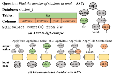
Figure 1: An example of grammar-based text-to-SQL.

To deal with the structured tree prediction, previous literature mainly utilizes classic LSTM network Hochreiter and Schmidhuber (1997) to construct the AST step-by-step. This common practice suffers from the following drawbacks: 1) unable to parallelize during training, and 2) incapable of modeling the complicated structure of AST. At each decoding timestep, the auto-regressive decoder chooses one unexpanded node in the partially-generated AST and expands it via restricted actions. Essentially, the process of decoding is a top-down traversal over all AST nodes (detailed in § 3). However, RNN is not specifically designed for structured tree generation and cannot capture the intrinsic connections. To compensate for the structural bias in the recurrent cell, TranX Yin and Neubig (2018) proposes parent feeding strategy, namely concatenating features of the parent node to the current decoder input. Although it achieves stable performance gain, other effective relationships such as siblings and ancestor-descendant are ignored. Besides, most previous work constructs the target AST in a canonical depth-first-search (DFS) left-to-right (L2R) order. In other words, the output action at each decoding timestep is pre-defined and fixed throughout training. It potentially introduces unreasonable permutation biases while traversing the structured AST and leads to the over-fitting problem with respect to generation order.

To this end, we propose an AST structure-aware Transformer decoder (ASTormer), and introduce more flexible decoding orders for text-to-SQL. By incorporating features of node types and positions into the Transformer decoder through both absolute and relative position embeddings Shaw et al. (2018), dedicated structure knowledge of the typed AST is integrated into the auto-regressive decoder ingeniously. It is also the process of symbol-to-neuron transduction. After computation in the neural space, the probabilistic output action is applied to the SQL AST. New nodes will be attached to the tree, which gives us updated structural information in the symbolic space. We experiment on five text-to-SQL benchmarks to validate our method, namely Spider Yu et al. (2018b), SParC Yu et al. (2019b), CoSQL Yu et al. (2019a), DuSQL Wang et al. (2020b) and Chase Guo et al. (2021). Performances demonstrate the effectiveness and efficiency of ASTormer compared to grammar-based LSTM-series decoders. To further verify its compatibility with different expanding orders of AST nodes, we try multiple decoding priors, e.g., DFS/breadth-first-search (BFS) and L2R/random selection. Experimental results prove that the proposed framework is insensitive towards different traversing sequences.

Main contributions are summarized as follows:

• A neural-symbolic ASTormer decoder is proposed which adapts the Transformer decoder to structured typed tree generation.

• We demonstrate that ASTormer is compatible with different traversing orders beyond depth-first-search and left-to-right (DFS+L2R).

• Experiments on multiple datasets verify the superiority of ASTormer over both grammar- and token-based models on the same scale.

2 Preliminaries

2.1 Problem Definition and Overview

Given a question $Q=(q_{1},q_{2},\cdots,q_{|Q|})$ with length $|Q|$ and the corresponding database schema $T\cup C$, the goal is to generate the SQL program $y$. The database schema contains multiple tables $T=\{t_{i}\}_{i=1}^{|T|}$ and columns $C=\{c_{i}\}_{i=1}^{|C|}$.

A grammar-based text-to-SQL parser follows the generic encoder-decoder Cho et al. (2014) architecture. The encoder converts all inputs into encoded states $\mathbf{X}=[\mathbf{Q};\mathbf{T};\mathbf{C}]\in\mathbb{R}^{(|Q|+|T|+|C|)\times d}$. Since it is not the main focus in this work, we assume $\mathbf{X}$ are obtained from a graph-based encoder, such as RATSQL Wang et al. (2020a).

Next, the decoder constructs the abstract syntax tree (AST) $y^{a}$ of SQL $y$ step-by-step via a sequence of actions $\boldsymbol{a}=(a_{1},a_{2},\cdots,a_{|a|})$. Each action $a_{j}$ chooses one unexpanded node in the incomplete tree $y^{a}_{j-1}$ and extends it through pre-defined semantics. The input of the decoder at each timestep is a typed node to expand, while the output is the corresponding action indicating how, see Figure 1(b). After the symbolic AST $y^{a}$ is completed, it is deterministically translated into SQL program $y$.

2.2 Basic Network Modules

Transformer Decoder Layer with Relative Position Embedding

Each ASTormer layer consists of $3$ cascaded sub-modules: 1) masked multi-head self-attention with relative position embedding (RPE), 2) multi-head cross attention, and 3) a feed-forward layer Vaswani et al. (2017), illustrated in the top right part of Figure 2. To incorporate target-side self-attention relations $\boldsymbol{z}_{ji}$ between each (query, key) pair $(\boldsymbol{n}_{j},\boldsymbol{n}_{i})$, we revise the computation of attention weight $\alpha_{ji}^{h}$ and context vector $\boldsymbol{\tilde{n}}_{j}^{h}$ like RPE Shaw et al. (2018): ($h$ is head index)

$$\alpha_{ji}^{h} =\underset{1\leq i\leq j}{\text{softmax}}\{\frac{(\boldsymbol{n}_{j}\mathbf{W}_{Q}^{h})(\boldsymbol{n}_{i}\mathbf{W}_{K}^{h}+\boldsymbol{z}_{ji})^{\mathrm{T}}}{\sqrt{d/H}}\},$$

$$\boldsymbol{\tilde{n}}^{h}_{j} =\sum_{1\leq i\leq j}\alpha^{h}_{ji}(\boldsymbol{n}_{i}\mathbf{W}^{h}_{V}+\boldsymbol{z}_{ji}),$$

Let $\mathbf{N}_{\leq j}=[\boldsymbol{n}_{1};\cdots;\boldsymbol{n}_{j}]$ denote the decoder input matrix, $\mathbf{X}=[\boldsymbol{x}_{1};\cdots;\boldsymbol{x}_{|X|}]$ denote the encoder cross-attention memory matrix and $\mathbf{Z}_{j}=\{\boldsymbol{z}_{ji}\}_{i=1}^{j}$ denote the set of relation features $\boldsymbol{z}_{ji}$ with timestep $i\leq j$, we formulate one ASTormer layer as:

$$\boldsymbol{n}_{j}^{\prime}= \text{ASTormerLayer}(\boldsymbol{n}_{j},\mathbf{N}_{\leq j},\mathbf{Z}_{j},\mathbf{X}).$$ (1)

Pointer Network

It is widely used to copy raw tokens from the input memory See et al. (2017). We re-use the multi-head cross-attention and take the average of weights $\alpha_{ji}^{h}$ from different heads $h$ as the probability of choosing the $i$-th entry in $\mathbf{X}$:

$$p_{\mathrm{ptr}}(i)= \frac{1}{H}\sum_{h}a_{ji}^{h},\quad h=1,\cdots,H,$$

$$= \text{PointerNetwork}(\boldsymbol{n}_{j},\mathbf{X})[i].$$

3 ASTormer Decoder

This section introduces our neural-symbolic ASTormer decoder which constructs the SQL AST $y^{a}$ given encodings $\mathbf{X}=[\mathbf{Q};\mathbf{T};\mathbf{C}]$. The framework is adapted from TranX Yin and Neubig (2018).

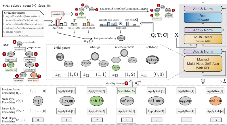
Figure 2: Illustration of ASTormer (the traversing order is DFS+L2R). We take the decoding timestep $j=4$ as an example. The lowest common ancestor for each node pair is highlighted with double border lines in the middle part.

3.1 Model Overview

The ASTormer decoder contains three modules: a frontier node input module (§ 3.3), a decoder hidden module of $L$ stacked ASTormer layers (§ 3.4), and an action output module (§ 3.5). At each decoding timestep $j$, it sequentially performs the following tasks to update the previous AST $y^{a}_{j-1}$.

1. Select one node $n_{j}$ to expand (called frontier node) from the frontier node set of $y^{a}_{j-1}$, and construct input feature $\boldsymbol{n}_{j}^{(0)}$ for it.

2. Further process node $n_{j}$ in the neural space by the decoder hidden module and get the final decoder state $\boldsymbol{n}_{j}$.

3. The action output module computes the distribution $P(a_{j})$ based on the type of node $n_{j}$.

4. Choose a valid action $a_{j}$ from $P(a_{j})$ and update $y^{a}_{j-1}$ in the symbolic space.

These steps are performed recurrently until no frontier node can be found in $y^{a}_{j}$. In other words, all nodes in $y^{a}_{j}$ have been expanded.

3.2 Basic Concepts of AST

To recap briefly, an abstract syntax tree (AST) is a tree representation of the source code.

Node type

Each node $n$ in the AST is assigned a type attribute $n^{\tau}$ representing its syntactic role. For example, in Figure 2, one node with type sql indicates the root of a complete SQL program. Nodes can be classified into non-terminal and terminal nodes based on their types. In this task, terminal types include tab_id, col_id, and tok_id, which denote the index of table, column, and tokens, respectively. Embeddings of each node type $n^{\tau}$ is provided by function $\psi(n^{\tau})\in\mathbb{R}^{1\times d}$.

Grammar rule

Each rule $r$ takes the form of

p$\_$type := RuleName(c$\_$type1, c$\_$type2,$\cdots$),

where p$\_$type is the type of the parent non-terminal node to expand, while (c$\_$type1, $\cdots$) denote types of children nodes to attach (can be duplicated or empty). Only non-terminal types can appear on the left-hand side of one rule. The complete set of grammar rules are list in Appendix A. We directly retrieve the feature of each grammar rule $r$ from an embedding function $\phi(r)\in\mathbb{R}^{1\times d}$.

3.3 Frontier Node Input Module

Given the chosen frontier node $n_{j}$, we need to firstly construct the input feature $\boldsymbol{n}_{j}^{(0)}$ at timestep $j$. It should reflect the information of node type and position in the AST to some extent. Thus, we initialize it as a sum of four vectors, including:

1. Previous action embedding $\boldsymbol{a}_{j-1}$ (defined in § 3.5), to inform the decoder of how to update the incomplete AST in the neural space.

2. Node type embedding $\psi(n^{\tau}_{j})$ of frontier node.

3. Parent rule embedding $\phi(r_{p_{j}})$, where $p_{j}$ denotes the timestep when the parent of node $n_{j}$ is expanded. This is similar to the parent feeding strategy in Yin and Neubig (2017).

4. Depth embedding $D^{a}(n_{j})\in\mathbb{R}^{1\times d}$ which indicates the depth of node $n_{j}$ in the AST $y^{a}_{j-1}$.

Notice that, vectors 2-4 serve as the original absolute position embeddings (APE) in Transformer decoder. We apply a LayerNorm Ba et al. (2016) layer upon the sum of these vectors. Formally,

$$\boldsymbol{n}_{j}^{(0)}=\text{LN}(\boldsymbol{a}_{j-1}+\psi(n^{\tau}_{j})+\phi(r_{p_{j}})+D^{a}(n_{j})).$$

3.4 Decoder Hidden Module

The initial node feature $\boldsymbol{n}_{j}^{(0)}$ is further processed by $L$ stacked ASTormer layers, see Eq.(1). The final decoder hidden state $\boldsymbol{n}_{j}$ is computed by

$$\boldsymbol{n}_{j}^{(l+1)} =\text{ASTormerLayer}^{(l)}(\boldsymbol{n}_{j}^{(l)},\mathbf{N}^{(l)}_{\leq j},\mathbf{Z}_{j},\mathbf{X}),$$

$$\boldsymbol{n}_{j} =\boldsymbol{n}_{j}^{(L)},\quad l=0,\cdots,L-1,$$

where $\mathbf{N}^{(l)}_{\leq j}$ denotes all node features $\boldsymbol{n}_{i}^{(l)}$ with timestep $i\leq j$ from the $l$-th decoder layer, and $\mathbf{Z}_{j}$ denotes all relational features $\boldsymbol{z}_{ji}$ from node $n_{j}$ to each previous node $n_{i}$. Borrowing the concept of lowest common ancestor (LCA) in data structure Bender et al. (2005), the relation $z_{ji}$ between each node pair $(n_{j},n_{i})$ is defined as a tuple:

$$\text{LCA}(n_{k},n_{s}) =\text{the LCA of node }n_{k}\text{ and }n_{s},$$

$$\text{dist}(n_{k},n_{s}) =\text{the distance between }n_{k}\text{ and }n_{s},$$

$$p_{j} =\text{dist}(\text{LCA}(n_{j},n_{i}),n_{j}),$$

$$p_{i} =\text{dist}(\text{LCA}(n_{j},n_{i}),n_{i}),$$

$$z_{ji}= (\text{clamp}(p_{j},R),\text{clamp}(p_{i},R)),$$ (2)

where $\text{clamp}(\cdot,R)$ truncates the maximum distance to $R$. Specifically, $z_{ji}=(1,0)$ implies that $n_{j}$ is a child of node $n_{i}$, while $z_{ji}=(1,1)$ denotes sibling relationships. By definition, $z_{ji}$ is symmetric in that if $z_{ji}=(2,3)$, the reverse relation must be $z_{ij}=(3,2)$. However, notice that some relations such as $z_{ji}=(0,1)$ will never be used, because a descendant node will not be expanded until all ancestors are done during the top-down traversal of AST. This topological constraint is fulfilled by the triangular future mask in self-attention.

Combining APE and RPE, the entire AST can be losslessly reconstructed through node types of endpoints and relative relations between any node pairs. For training, these information can be pre-extracted once and for all. During inference, the relation $Z_{j}$ can be efficiently constructed on-the-fly via dynamic programming due to the symmetric definition of $z_{ji}$ and acyclic property of AST (detailed in Appendix B).

3.5 Action Output Module

Given decoder state $\boldsymbol{n}_{j}$, the next step is to compute the distribution $P(a_{j})$ of output actions based on the node type $n^{\tau}_{j}$. As illustrated in Figure 3, there are three genres of actions: 1) ApplyRule$[r]$ for non-terminal types, 2) SelectItem$[i]$ for terminal types tab_id and col_id (Item$\in$$\{$Table, Column$\}$), and 3) GenToken for tok_id.

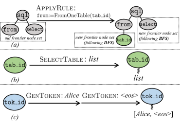
Figure 3: Three types of actions and their semantics.

ApplyRule Action

This action chooses one rule $r_{i}$ from a constrained set of grammar rules determined by the non-terminal type $n^{\tau}_{j}$. Specifically, the left-hand side of grammar rule $r_{i}$ must equal $n^{\tau}_{j}$ (known as node type constraint, Krishnamurthy et al., 2017). When applying this action to AST $y_{j-1}^{a}$ in the symbolic space, we attach all children types on the right-hand side of rule $r_{i}$ to the parent node $n_{j}$ and mark these children nodes as unexpanded. Given $\boldsymbol{n}_{j}$, the distribution of ApplyRule action is calculated by

$$P(a_{j}=\textsc{ApplyRule}[r_{i}]|a_{<j},\boldsymbol{n}_{j},\mathbf{X})=\\ \underset{i}{\text{softmax}}\{\boldsymbol{n}_{j}\mathbf{W}_{\text{ar}}\phi(r_{i})^{\textrm{T}}\}.$$

SelectItem Action

Taking SelectTable action as an example, to expand frontier node with terminal type tab$\_$id, we directly choose one table entry and attach it to the input terminal node. The probability of selecting the $i$-th entry from encoded table memory $\mathbf{T}\in\mathbb{R}^{|T|\times d}$ is computed by

$$P(a_{j}=\textsc{SelectTable}[t_{i}]|a_{<j},\boldsymbol{n}_{j},\mathbf{X})=\\ \text{PointerNetwork}_{\text{st}}(\boldsymbol{n}_{j},\mathbf{T})[i].$$

GenToken Action

To produce SQL values for terminal node of type tok_id, we utilize the classic pointer-generator network See et al. (2017). Raw token $w_{i}$ can be generated from a vocabulary or copied from the input question memory $\mathbf{Q}\in\mathbb{R}^{|Q|\times d}$. Mathematically,

$$g_{j} =\text{sigmoid}([\boldsymbol{n}_{j}\circ\boldsymbol{n}_{j}^{(0)}]\mathbf{W}_{\text{g}}),$$

$$P_{\text{gen}}(w_{i}) =\underset{i}{\text{softmax}}\{\boldsymbol{n}_{j}\mathbf{W}_{\text{gen}}e(w_{i})^{\mathrm{T}}\},$$

$$P_{\text{copy}}(w_{i}) =\sum_{k:\ q_{k}=w_{i}}\text{PointerNetwork}_{\text{gt}}(\boldsymbol{n}_{j},\mathbf{Q})[k],$$

$$\begin{split}P(a_{j}&=\textsc{GenToken}[w_{i}]|a_{<j},\boldsymbol{n}_{j},\mathbf{X})=\\ &\quad g_{j}P_{\text{gen}}(w_{i})+(1-g_{j})P_{\text{copy}}(w_{i}),\end{split}$$

where $g_{j}\in[0,1]$ is the balance score and $e(w_{i})\in\mathbb{R}^{1\times d}$ denotes the word embedding of token $w_{i}$. Since each SQL value may have multiple tokens, node $n_{j}$ is not expanded until a special “<eos>" token is emitted. Intermediate results are buffered and the frontier node chosen at timestep $j+1$ is still $n_{j}$ if the current output action $a_{j}$ is not “<eos>". After the emission of “<eos>", we extend node $n_{j}$ by attaching the list of all buffered tokens.

Until now, the action embedding $\boldsymbol{a}_{j}\in\mathbb{R}^{1\times d}$ (as decoder input for the next timestep) can be defined,

$$\boldsymbol{a}_{j}=\begin{cases}\phi(r_{j})&\text{if }a_{j}\in\textsc{ApplyRule}\\ \boldsymbol{t}_{j}\text{ or }\boldsymbol{c}_{j}&\text{if }a_{j}\in\textsc{SelectItem}\\ e(w_{j})&\text{if }a_{j}\in\textsc{GenToken}\end{cases},$$

where $r_{j}$/$w_{j}$ is the rule/token chosen at the current timestep $j$, and $\boldsymbol{t}_{j}$/$\boldsymbol{c}_{j}$ is the selected entry in table/column memory $\mathbf{T}$/$\mathbf{C}$. Parameters of $\text{PointerNetwork}_{\ast}(\boldsymbol{n}_{j},\cdot)$ are shared among SelectTable, SelectColumn, and GenToken actions to avoid over-parametrization.

The prediction of the SQL AST $y^{a}$ can be decoupled into a sequence of actions $\boldsymbol{a}=(a_{1},\cdots,a_{|a|})$. The training objective for the text-to-SQL task is

$$\mathcal{L}=-\sum_{j=1}^{|a|}\log P(a_{j}|a_{<j},\mathbf{X}).$$ (3)

3.6 Different Traversal Paths

What remains to be resolved is 1) how to update the frontier node set given a new action $a_{j}$, and 2) choose one input frontier node $n_{j}$ from this set.

3.6.1 Update Frontier Node Set: DFS or BFS

The frontier node set refers to a restricted set of unexpanded nodes in the incomplete AST $y^{a}_{j-1}$ that we focus on currently. It is usually constrained and implemented by depth-first-search (DFS) or breadth-first-search (BFS). If DFS is strictly followed, the sets of unexpanded nodes can be stored as a stack. Each element in the stack is a set of unexpanded nodes. After applying action $a_{j}$ to frontier node $n_{j}$, we remove $n_{j}$ from the node set at the top of stack and push the set of its children nodes (if not empty) onto the stack. By analogy, if the AST traversal order is breadth-first-search (BFS), we only need to maintain a first-in-first-out queue. For example, in Figure 3(a), after expanding node “from”, the updated frontier node set is the singleton set which contains node “tab_id” if DFS is followed (otherwise node “select” if BFS). Note that, if $n_{j}^{\tau}={\tt tok\_id}$ and the current output action $a_{j}\neq\textsc{GenToken}[\text{<eos>}]$, the frontier node $n_{j}$ is preserved and forced to be chosen next.

3.6.2 Choose Frontier Node: L2R or Random

To select frontier node from the restricted set, a common practice Guo et al. (2019) is to stipulate a canonical order, also known as left-to-right (L2R). For example, given the grammar rule sql := FromSelect(from, select), the model always expands node “from” prior to “select". Evidently, this pre-defined priority abridges the freedom in AST construction. In this work, we attempt to eliminate this constraint and propose a more intuitive Random method. Concretely, during training, we randomly sample one frontier node from the node set at top of stack (or head of queue). Such randomness prevents the model from over-fitting the permutation bias and inspires the decoder to truly comprehend the relative positions $z_{ji}$ of different node pairs. As for inference, instead of choosing one candidate from the frontier node set at each timestep, all distinct options are enumerated as inputs to the decoder to enlarge the search space. This relaxation encourages the model itself to discover the optimal traversal path and provides more interpretation on the neural-symbolic processing.

Due to page limit, more details and the complete algorithm are elaborated in Appendix C.

4 Experiments

Category	Method	PLM	Spider		SParC		CoSQL
			EM	EX	QM	IM	QM	IM
token-based	EditSQL Zhang et al. (2019)	BERT Devlin et al. (2019)	57.6	-	47.2	29.5	39.9	12.3
	GAZP Zhong et al. (2020b)		59.1	59.2	48.9	29.7	42.0	12.3
	IGSQL Cai and Wan (2020)		-	-	50.7	32.5	44.1	15.8
grammar-based	RATSQL Wang et al. (2020a)	BERT	69.7	-	-	-	-	-
	R2SQL Hui et al. (2021)		-	-	54.1	35.2	45.7	19.5
Ours	RATSQL w/ LSTM	BERT	70.1	67.2	58.7	38.2	49.1	18.1
	RATSQL w/ ASTormer		71.7	70.4	61.6	39.8	49.9	18.4
token-based	UnifiedSKG Xie et al. (2022)	T5-Large Raffel et al. (2020)	67.6	-	59.0	-	51.6	-
	UniASr Dou et al. (2022)	BART Lewis et al. (2020)	70.0	60.4	60.4	40.8	51.8	21.3
grammar-based	RATSQL	GraPPa Yu et al. (2020a)	73.6	-	-	-	-	-
	RATSQL	SCoRe Yu et al. (2020b)	-	-	62.2	42.5	52.1	22.0
	HIESQL Zheng et al. (2022)	GraPPa Yu et al. (2020a)	-	-	64.7	45.0	56.4	28.7
Ours	RATSQL w/ LSTM	ELECTRA Clark et al. (2020)	72.9	71.4	62.8	41.2	52.9	22.5
	RATSQL w/ ASTormer		74.6	73.2	64.8	45.0	55.5	22.9

Table 1: Main results on three English benchmarks. For fairness, we compare results with those using PLMs on the same scale. We do not utilize any reranking, regularization, data augmentation, and ensemble methods.

4.1 Experimental Setup

Datasets

We experiment on $5$ typical text-to-SQL benchmarks. Spider Yu et al. (2018b) is a large-scale, cross-domain, multi-table English benchmark for text-to-SQL. SparC Yu et al. (2019b) and CoSQL Yu et al. (2019a) are multi-turn versions. To compare ASTormer with models in the literature, we report official metrics on development sets (EM and EX accuracy for Spider, QM and IM for SParC and CoSQL), since test sets are not publicly available. For results on Chinese datasets such as DuSQL Wang et al. (2020b) and Chase Guo et al. (2021), see Appendix E for details.

Our model is implemented with Pytorch Paszke et al. (2019) . PLM and its initial checkpoint are downloaded from the transformers Wolf et al. (2020) library. For the graph encoder, we reproduce the prevalent RATSQL Wang et al. (2020a). The hidden dimension $d$ is $512$ and the number of encoder/decoder layers is $8$/$2$. The number of heads and dropout rate is set to $8$ and $0.2$ respectively. Throughout the experiments, we use AdamW Loshchilov and Hutter (2019) optimizer with a linear warmup scheduler. The warmup ratio of total training steps is $0.1$. The leaning rate is $4e\textrm{-}4$ (small), $2e\textrm{-}4$ (base) or $1e\textrm{-}4$ (large) for PLMs of different sizes and the weight decay rate is fixed to $0.1$. The optimization of PLM parameters is carried out more carefully with learning rate layerwise decay (coefficient $0.8$). Batch size is $20$, and the number of training iterations is $100k$. For inference, we adopt beam search with size $5$.

4.2 Main Results

Main results are provided in Table 1. Some conclusions can be summarized: 1) Our ASTormer decoder consistently outperforms the LSTM decoder across all three benchmarks on both metrics. For example, with ELECTRA Clark et al. (2020), ASTormer beats traditional LSTM decoder by $1.7$ points on Spider in metric EM, while $2$ or more points on SParC and CoSQL. Moreover, we compute the average training time per $100$ iterations for LSTM and ASTormer decoders in Table 2. Not surprisingly, ASTormer is three times faster (even four times on Spider due to longer action sequences) than LSTM decoder. Although it introduces some overheads about structural features, the overall training time is still comparable to token-based Transformer on account of shorter output sequences. That is, the average number of AST nodes is smaller than that of tokenized SQL queries, see Appendix D for dataset statistics. 2) Arguably, grammar-based decoders are superior to token-based methods among models on the same scale. It can be explained that grammar-based methods explicitly inject the structure knowledge of SQL programs into the decoder. Although recent advanced token-based models such as PicardScholak et al. (2021b) and RASATQi et al. (2022) show exciting progress, they heavily rely on large PLMs, which may be unaffordable for some research institutes. Thus, lightweight grammar-based models provide a practical solution in resource-constrained scenarios. 3) Equipped with more powerful PLMs tailored for structured data, performances can be further promoted stably. Accordingly, we speculate those task-adaptive PLMs which focus on enhancing the discriminative capability are more suitable in text-to-SQL. The evidence is that PLMs such as GraPPa Yu et al. (2020a), SCoRe Yu et al. (2020b), and ELECTRA Clark et al. (2020), all design pre-training tasks like syntactic role classification and word replacement discrimination. Pre-training on large-scale semi-structured tables is still a long-standing and promising direction.

Dataset	Category	Cell	Acc.	Time/$sec.$
Spider	token-based	Transformer	$69.7$	$49.5$
2-5[1pt/1pt]	grammar-based	LSTM	$69.9$	$191.4$
		ASTormer	$71.4$	$45.8$$(\times 4.2)$
SParC	token-based	Transformer	$59.8$	$49.1$
2-5[1pt/1pt]	grammar-based	LSTM	$60.9$	$168.1$
		ASTormer	$61.3$	$49.8$$(\times 3.4)$
CoSQL	token-based	Transformer	$50.1$	$52.8$
2-5[1pt/1pt]	grammar-based	LSTM	$50.5$	$154.2$
		ASTormer	$51.1$	$60.7$$(\times 2.5)$

Table 2: Acc. and avg. training time (seconds) per $100$ iterations with PLM electra-small. We also implement a token-based Transformer decoder with question copy and schema selection mechanism See et al. (2017).

4.3 Ablation Studies

For the sake of memory space, the following experiments are conducted with PLM electra-small unless otherwise specified.

Method	Spider	SParC	CoSQL
ASTormer	71.4	61.3	51.1
w/o node type	70.9$(0.5\downarrow)$	58.5$(2.8\downarrow)$	48.3$(2.8\downarrow)$
w/o parent rule	69.0$(2.4\downarrow)$	58.6$(2.7\downarrow)$	49.4$(1.7\downarrow)$
w/o node depth	70.1$(1.3\downarrow)$	58.2$(3.1\downarrow)$	47.1$(4.0\downarrow)$
w/ pe	69.0$(2.4\downarrow)$	58.9$(2.4\downarrow)$	48.9$(2.2\downarrow)$
w/o relations	69.7$(1.7\downarrow)$	58.9$(2.4\downarrow)$	48.1$(3.0\downarrow)$
w/ rpe $j-i$	69.4$(2.0\downarrow)$	58.2$(3.1\downarrow)$	48.9$(2.2\downarrow)$
Transformer	68.2$(3.2\downarrow)$	57.3$(4.0\downarrow)$	47.5$(3.6\downarrow)$

Table 3: Ablation of different components in ASTormer. “pe”/“rpe” represents traditional absolute and relative position embeddings respectively; “Transformer” denotes an AST decoder which only utilizes previous action embedding and position embedding.

Size of $R$	2	4	8	16	Max Tree Depth
Spider	69.9	71.3	71.4	70.4	16
SParC	60.8	61.3	60.4	61.2	10
CoSQL	49.8	51.1	50.3	50.0	10

Table 4: Ablation of the maximum relative distance $R$.

Ablation of Structural Features

In Table 3, we analyze the contribution of each module in ASTormer, including the node type embedding $\psi(n_{j}^{\tau})$, the parent rule embedding $\phi(r_{p_{j}})$, the node depth embedding $D^{a}(n_{j})$, and the relative positions between node pairs $z_{ji},i\leq j$. From the overall results, we can find that the performance undoubtedly declines no matter which component is omitted. When we replace the node depth/relations $z_{ji}$ with traditional absolute/relative position embeddings, the performance still decreases. It demonstrates that traditional position embeddings are not suitable in structured tree generation and may introduce incorrect biases. When we remove all structural features, the proposed ASTormer decoder degenerates into purely Transformer-based AST decoder. Unfortunately, it also gives the worst performances, which validates the significance of integrating structure knowledge into the decoder from the opposite side.

Impact of Number of Relations

Next, we attempt to find the optimal number of relation types. As defined in Eq.(2), threshold $R$ is used to truncate the maximum distance between node $n_{j}$ and the lowest common ancestor of $(n_{j},n_{i})$. Notice that, the number of total relation types increases at a square rate as the threshold $R$ gets larger. The original problem is reduced to find a suitable threshold $R$. Intuitively, the optimal threshold is tightly related to both the shape and size of SQL ASTs. We calculate the maximum tree depth for each dataset in the last column of Table 4. By varying the size of $R$, we discover that one feasible choice is to set $R$ as roughly half of the maximum tree depth.

Decoding Order	Spider	Sparc	CoSQL
DFS+L2R	68.5	58.6	48.7
DFS+Random	68.6	58.1	48.5
BFS+L2R	68.2	58.2	48.9
BFS+Random	68.0	57.2	47.1

Table 5: Ablation of different traversal orders. DFS: depth-first-search; BFS: breadth-first-search; L2R: left-to-right; Random: random sampling during training.

Different Traversal Orders

We also compare $4$ different choices depending on how to update the frontier node set (DFS or BFS) and how to select frontier node from this set (L2R or Random), detailed in § 3.6 and Appendix C.2. According to Table 5, we can safely conclude that: benefiting from the well-designed structure, different orders does not significantly influence the eventual performance (even with Random method which evidently enlarges the search space). Furthermore, we can take advantage of the self-adaptive node selection and mark AST nodes with decoding timestamps during inference. It provides better symbolic interpretation on the decoding process. Through case studies (partly illustrated in Table 6), we find that in roughly $76.2\%$ cases, the model prefers to expand node “from” before “select” where only one table is required in the target SQL. This observation is consistent with previous literature Lin et al. (2020) that prioritizing From clause according to the execution order is superior to the written order that Select clause comes first. However, this ratio decreases to $13.9\%$ when it encounters the JOIN of multiple tables. In this situation, we speculate that the model tends to identify the user intents (Select clause) and requirements (Where clause) first according to the input question, and switch to the complicated construction of a connected table view based on the database schema graph. More examples are provided in Appendix F.

DB: concert_singer

Question: How many singers do we have?

SQL: select count(*) from singer

SQL AST:

sql $\rightarrow$ Node[ $j=0$, sql := SQL(from, select, condition, groupby, orderby) ]

groupby $\rightarrow$ Node[ $j=1$, groupby := NoGroupBy() ]

from $\rightarrow$ Node[ $j=2$, from := FromTableOne(tab_id, condition) ]

tab_id $\rightarrow$ Leaf[ $j=3$, tab_id := singer ]

condition $\rightarrow$ Node[ $j=4$, condition := NoCondition() ]

condition $\rightarrow$ Node[ $j=5$, condition := NoCondition() ]

select $\rightarrow$ Node[ $j=6$, select := SelectColumnOne(distinct, col_unit) ]

distinct $\rightarrow$ Node[ $j=7$, distinct := False() ]

col_unit $\rightarrow$ Node[ $j=8$, col_unit := UnaryColumnUnit(agg_op, distinct, col_id) ]

distinct $\rightarrow$ Node[ $j=9$, distinct := False() ]

agg_op $\rightarrow$ Node[ $j=10$, agg_op := Count() ]

col_id $\rightarrow$ Leaf[ $j=11$, col_id := * ]

orderby $\rightarrow$ Node[ $j=12$, orderby := NoOrderBy() ]

DB: poker_player

Question: What are the names of poker players?

SQL: select T1.Name from people as T1 join poker_player as T2 on T1.People_ID = T2.People_ID

SQL AST:

sql $\rightarrow$ Node[ $j=0$, sql := SQL(from, select, condition, groupby, orderby) ]

select $\rightarrow$ Node[ $j=1$, select := SelectColumnOne(distinct, col_unit) ]

distinct $\rightarrow$ Node[ $j=2$, distinct := False() ]

col_unit $\rightarrow$ Node[ $j=3$, col_unit := UnaryColumnUnit(agg_op, distinct, col_id) ]

agg_op $\rightarrow$ Node[ $j=4$, agg_op := None() ]

distinct $\rightarrow$ Node[ $j=5$, distinct := False() ]

col_id $\rightarrow$ Leaf[ $j=6$, col_id := people.Name ]

condition $\rightarrow$ Node[ $j=7$, condition := NoCondition() ]

groupby $\rightarrow$ Node[ $j=8$, groupby := NoGroupBy() ]

from $\rightarrow$ Node[ $j=9$, from := FromTableTwo(tab_id, tab_id, condition) ]

tab_id $\rightarrow$ Leaf[ $j=10$, tab_id := poker_player ]

tab_id $\rightarrow$ Leaf[ $j=11$, tab_id := people ]

condition $\rightarrow$ Node[ $j=12$, condition := CmpCondition(col_unit, cmp_op, value) ]

col_unit $\rightarrow$ Node[ $j=13$, col_unit := UnaryColumnUnit(agg_op, distinct, col_id) ]

distinct $\rightarrow$ Node[ $j=14$, distinct := False() ]

agg_op $\rightarrow$ Node[ $j=15$, agg_op := None() ]

col_id $\rightarrow$ Leaf[ $j=16$, col_id := poker_player.People_ID ]

cmp_op $\rightarrow$ Node[ $j=17$, cmp_op := Equal() ]

value $\rightarrow$ Node[ $j=18$, value := ColumnValue(col_id) ]

col_id $\rightarrow$ Leaf[ $j=19$, col_id := people.People_ID ]

orderby $\rightarrow$ Node[ $j=20$, orderby := NoOrderBy() ]

Table 6: Case study on traversal order using method DFS+Random on Spider Yu et al. (2018b). $j$ represents the decoding timestep when the node is expanded.

5 Related Work

Text-to-SQL Decoding

SQL programs exhibit strict syntactic and semantic constraints. Without restriction, the decoder will waste computation in producing ill-formed programs. To tackle this constrained decoding problem, existing methods can be classified into two categories: token-based and grammar-based. 1) A token-based decoder Lin et al. (2020); Scholak et al. (2021b) directly generates each token in the SQL autoregressively. This method requires syntax- or execution-guided decoding Wang et al. (2018) to periodically eliminate invalid partial programs from the beam during inference. 2) A grammar-based decoder Krishnamurthy et al. (2017); Yin and Neubig (2017); Guo et al. (2019) predicts a sequence of actions (or grammar rules) to construct the equivalent SQL AST instead. Type constraints Krishnamurthy et al. (2017) can be easily incorporated into node types and grammar rules. In this branch, both top-down (IRNet, Guo et al., 2019) and bottom-up (SmBoP, Rubin and Berant, 2021) grammars have been applied to instruct the decoding. We focus on the grammar-based category and propose an AST decoder which is compatible with Transformer.

Structure-aware Decoding

Various models have been proposed for structured tree generation, such as Asn Rabinovich et al. (2017), TranX Yin and Neubig (2018), and TreeGen Sun et al. (2020). These methods introduce complex shortcut connections or specialized modules to model the structure of output trees. In contrast, StructCoder Tipirneni et al. (2022) still adopts the token-based paradigm and devises two auxiliary tasks (AST paths and data flow prediction) during training to encode the latent structure into objective functions. Peng et al. (2021) also integrates tree path encodings into attention module, but they work on the encoding part and assume that the complete AST is available. In this work, we propose a succinct ASTormer architecture for the decoder and construct the SQL AST on-the-fly during inference.

6 Conclusion

In this work, we propose an AST structure-aware decoder for text-to-SQL. It integrates the absolute and relative position of each node in the AST into the Transformer decoder. Extensive experiments verify that ASTormer is more effective and efficient than traditional LSTM-series AST decoder. And it can be easily adapted to more flexible traversing orders. Future work includes extending ASTormer to more general situations like graph generation.

Limitations

In this work, we mainly focus on grammar-based decoders for text-to-SQL. Both token-based parsers equipped with relatively larger pre-trained language models such as T5-3B Raffel et al. (2020) and prompt-based in-context learning methods with large language models such as ChatGPT Ouyang et al. (2022) are beyond the scope, since this paper is restricted to local interpretable small-sized models (less than 1B parameters) which are cheaper and faster.

Appendix A Grammar Rules

In Table 8, we provide the complete set of grammar rules for SQL AST parsing. This specification conforms to a broader category called abstract syntax description language (ASDL, Wang et al., 1997). Take the following grammar rule as an example:

$${\tt select}:=\\ \text{SelectOneColumn}({\tt distinct},{\tt col\_unit}),$$

the corresponding ApplyRule action will expand the non-terminal node of type “select”. Concretely, two unexpanded children nodes of types “distinct” and “col_unit” will be attached to the parent node of type “select”.

Appendix B Construction of Relations On-the-fly

In this part, we introduce how to construct the relation set $Z_{j}=\{z_{ji}\}_{i=1}^{j}$ at timestep $j$ given all previous relation sets $Z_{<j}$ during inference. The entire set $Z_{j}$ can be divided into three parts:

$$Z_{j}= Z_{j}^{0}\bigcup Z_{j}^{1}\bigcup Z_{j}^{2},$$

$$= \{z_{jj}\}\bigcup\{z_{ji}\}_{i=1}^{p_{j}}\bigcup\{z_{ji}\}_{i=p_{j}+1}^{j-1},$$

where $p_{j}$ denotes the timestep when the parent of the current frontier node $n_{j}$ is expanded ($p_{j}<j$).

• For $Z_{j}^{0}=\{z_{jj}\}$, we directly use $z_{jj}=(0,0)$.

• For each $z_{ji}\in Z_{j}^{1}=\{z_{ji}\}_{i=1}^{p_{j}}$, we retrieve the corresponding relation $z_{p_{j}i}\in Z_{p_{j}}$ with the same index $i$. Assume that $z_{p_{j}i}=(k,s)$, then $z_{ji}$ must be

  $$z_{ji}=(\text{clamp}(k+1,R),s).$$

• For each $z_{ji}\in Z_{j}^{2}=\{z_{ji}\}_{i=p_{j}+1}^{j-1}$, although $z_{p_{j}i}\notin Z_{p_{j}}$, the counter-part $z_{ip_{j}}$ must be already constructed in $Z_{i}$ with $p_{j}<i<j$. Assume that $z_{ip_{j}}=(k,s)$, considering the symmetric definition of relations, $z_{ji}$ must be

  $$z_{ji}=(\text{clamp}(s+1,R),k).$$

Based on the three rules above, the relation set $Z_{j}$ at each timestep can be efficiently computed with little overheads. An empirical comparison with LSTM-based AST decoder on inference time is presented in Table 7.

Dataset	Spider	SParC	CoSQL
LSTM	206.6	191.5	201.0
ASTormer	237.0	200.7	199.1

Table 7: Inference time comparison (seconds/per $1000$ samples under the same configuration).

Terminal types:

tab_id, col_id, tok_id

Grammar rules for non-terminal types:

sql := Intersect(sql, sql) $|$ Union(sql, sql) $|$ Except(sql, sql) $|$ SQL(from, select, condition, groupby, orderby)

select := SelectOneColumn(distinct, col_unit) $|$ SelectTwoColumn(distinct, col_unit, col_unit) $|$ $\cdots$

from := FromOneSQL(sql) $|$ FromTwoSQL(sql, sql) $|$ $\cdots$

$|$ FromOneTable(tab_id) $|$ FromTwoTable(tab_id, tab_id, condition) $|$ $\cdots$

groupby := NoGroupBy

$|$ GroupByOneColumn(col_id, condition) $|$ GroupByTwoColumn(col_id, col_id, condition) $|$ $\cdots$

orderby := NoOrderBy

$|$ OrderByOneColumn(col_unit, order) $|$ OrderByTwoColumn(col_unit, col_unit, order) $|$ $\cdots$

$|$ OrderByLimitOneColumn(col_unit, order, tok_id) $|$ OrderByLimitTwoColumn(col_unit, col_unit, order, tok_id) $|$ $\cdots$

order := Asc $|$ Desc

condition := NoCondition

$|$ AndTwoCondition(condition, condition) $|$ AndThreeCondition(condition, condition, condition) $|$ $\cdots$

$|$ OrTwoCondition(condition, condition) $|$ OrThreeCondition(condition, condition, condition) $|$ $\cdots$

$|$ BetweenCondition(col_unit, value, value)

$|$ CmpCondition(col_unit, cmp_opvalue)

cmp_op := Equal $|$ NotEqual $|$ GreaterThan $|$ GreaterEqual $|$ LessThan $|$ LessEqual $|$ Like $|$ NotLike $|$ In $|$ NotIn

value := SQLValue(sql) $|$ LiteralValue(tok_id) $|$ ColumnValue(col_id)

col_unit := UnaryColumnUnit(agg_op, distinct, col_id) $|$ BinaryColumnUnit(agg_op, unit_op, col_id, col_id)

distinct := True $|$ False

agg_op := None $|$ Max $|$ Min $|$ Count $|$ Sum $|$ Avg

unit_op := Minus $|$ Plus $|$ Times $|$ Divide

Table 8: The checklist of all grammar rules used throughout all experiments. “$|$” is the separator for different rule constructors. “$\cdots$” means part of the quantitive grammar rules are omitted which can be easily inferred, and the maximum number of children types is determined by statistics of the training set. Note that grammar rules such as “order := Asc $|$ Desc” denote no children node will be attached to the parent.

Appendix C Details of Different Traversal Paths

C.1 Modeling of AST Construction

To construct the SQL AST $y^{a}$ in an auto-regressive fashion, there are multiple top-down traversal paths $\mathcal{T}(y^{a})$. Each traversal path $\rho\in\mathcal{T}(y^{a})$ can be further decoupled into the sequence of (AST node, output action) pairs $\rho=\bigl{(}(n_{1},a_{1}),\cdots,(n_{|y^{a}|},a_{|y^{a}|})\bigl{)}$. The probabilistic modeling is formulated as:

$$\log P(y^{a})= \sum_{\rho\in\mathcal{T}(y^{a})}\log P(\rho)$$

$$= \sum_{\rho\in\mathcal{T}(y^{a})}\log P(n_{1},a_{1},\cdots,n_{|y^{a}|},a_{|y^{a}|})$$

$$= \sum_{\rho\in\mathcal{T}(y^{a})}\sum_{j=1}^{|y^{a}|}\log P(n_{j},a_{j}|n_{<j},a_{<j})$$

$$= \sum_{\rho\in\mathcal{T}(y^{a})}\sum_{j=1}^{|y^{a}|}\bigl{(}\log P(n_{j}|n_{<j},a_{<j})$$

$$\qquad\qquad\quad+\log P(a_{j}|n_{\leq j},a_{<j})\bigl{)},$$

where the conditioning on input $\mathbf{X}$ is omitted for brevity. Given a specific traversal path $\rho$, the modeling of $\log P(n_{j},a_{j}|n_{<j},a_{<j})$ at each timestep $j$ is divided into two parts:

$$\underbrace{\log P(n_{j}|n_{<j},a_{<j})}_{\text{selection of frontier node }n_{j}}+\underbrace{\log P(a_{j}|n_{\leq j},a_{<j})}_{\text{modeling of output action }a_{j}}.$$

The first part gives the distribution of choosing one unexpanded node in $y^{a}_{j-1}$, while the second part is exactly the output of the AST decoder.

Most previous work simplifies the first part by assuming one canonical traversal path (DFS+L2R) given AST $y^{a}$. In other words, $\mathcal{T}_{\text{dfs}}^{\text{l2r}}(y^{a})$ is a singleton set containing merely one unrolled path, and $P(n_{j}|n_{<j},a_{<j})$ is a unit mass distribution where only the leftmost node in the frontier node set restricted by DFS has the probability $1$ (similarly for $\mathcal{T}_{\text{bfs}}^{\text{l2r}}(y^{a})$). In this case, we only need to care about the distribution of output actions since each frontier node $n_{j}$ is uniquely determined by $y^{a}_{j-1}$. It gives us exactly the training objective in Eq.(3):

$$\log P(y^{a})= \sum_{j=1}^{|y^{a}|}\log P(a_{j}|n_{<j},a_{<j})$$

$$= \sum_{j=1}^{|y^{a}|}\log P(a_{j}|a_{<j}).$$

In this work, we relax the permutation prior injected in the “horizontal” direction (not necessarily L2R) and propose the Random method (§ 3.6). Concretely, the entire set of acceptable traversal paths is restricted by DFS (or BFS), and the total number of paths in $\mathcal{T}_{\text{dfs}}(y^{a})$ (or $\mathcal{T}_{\text{bfs}}(y^{a})$) equals to

$$|\mathcal{T}_{\text{dfs}}(y^{a})|=|\mathcal{T}_{\text{bfs}}(y^{a})|=\prod_{n_{i}\in y^{a}}|\text{Children}(n_{i})|!\ ,$$

where $|\text{Children}(n_{i})|$ denotes the number of children for each node $n_{i}$ in AST $y^{a}$. An illustration of different traversal paths $\mathcal{T}_{\text{dfs}}(y^{a})$ and its cardinality is provided in Figure 4. Assume that each path $\rho$ has equal prior, then the selection of frontier node $P(n_{j}|n_{<j},a_{<j})$ is a uniform distribution over the current frontier node set restricted by DFS (or BFS). And the computation of $\log P(y^{a})$ can be reduced to: (take DFS as an example)

$$\log P(y^{a})= \sum_{\rho\in\mathcal{T}_{\text{dfs}}(y^{a})}\Bigl{(}\sum_{j=1}^{|y^{a}|}\log P(n_{j}|n_{<j},a_{<j})$$

$$\qquad\quad+\sum_{j=1}^{|y^{a}|}\log P(a_{j}|n_{\leq j},a_{<j})\Bigl{)}$$

$$= \sum_{\rho\in\mathcal{T}_{\text{dfs}}(y^{a})}\Bigl{(}\log\frac{1}{\prod_{n_{i}\in y^{a}}|\text{Children}(n_{i})|!}$$

$$\qquad\quad+\sum_{j=1}^{|y^{a}|}\log P(a_{j}|n_{\leq j},a_{<j})\Bigl{)}$$

$$= c+\sum_{\rho\in\mathcal{T}_{\text{dfs}}(y^{a})}\sum_{j=1}^{|y^{a}|}\log P(a_{j}|n_{\leq j},a_{<j}),$$

where $c$ is a constant value irrelevant of $\rho$ and only dependent on the shape of $y^{a}$. Considering enormous traversal paths in $\mathcal{T}_{\text{dfs}}(y^{a})$, we adopt uniform sampling during training and enlarge the search space over frontier nodes $n_{j}$ during inference (detailed in Appendix C.2).

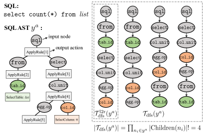
Figure 4: Illustration of different traversal paths $\mathcal{T}_{\text{dfs}}(y^{a})$ re-using the same example in Figure 2.

C.2 Training and Inference Algorithms

Algorithm 1 Generic Training Algorithm

1:Labeled AST $y^{a}$; Encoder output $\mathbf{X}=[\mathbf{Q};\mathbf{T};\mathbf{C}]$; Order method $m$;

2:Training loss $\mathcal{L}$ for one sample;

3:traverse AST $y^{a}$ via DFS/BFS+L2R and record necessary information for each node, including traverse timestep $j$, node type $n_{j}^{\tau}$, parent grammar rule $r_{p_{j}}$, node depth $D^{a}(n_{j})$ and output action $a_{j}$;

4:construct the relational matrix $Z=\{z_{ji}\}_{1\leq i,j\leq|y^{a}|}$ for each node pair in $y^{a}$;

5:

6:if $m\in\{\text{DFS+Random, BFS+Random}\}$ then $\triangleright$ only “Random” needs sampling and permutation

7:     sample a traversal path over $y^{a}$ following $m$ and record timestamps;

8:     permute the $1$-dimension sequence of $(n_{j}^{\tau},r_{p_{j}},D^{a}(n_{j}),a_{j})$ based on timestamps;

9:     permute the relation matrix $Z$ twice in two dimensions based on timestamps;

10:end if

11:

12:compute training loss $\mathcal{L}$ in parallel given $\mathbf{X}$, the current traversal sequence and relation matrix $Z$;

13:return training loss $\mathcal{L}$

Algorithm 2 Generic Inference Algorithm

1:Encoder output $\mathbf{X}=[\mathbf{Q};\mathbf{T};\mathbf{C}]$; Beam size $K$; Order method $m$; Max decoding steps $M$;

2:Predicted SQL program $\hat{y}$;

3:initialize AST $y_{0}^{a}$ with a single node of root type “sql”;

4:initialize beam $\mathcal{B}_{0}=\{y^{a}_{0}\}$ with one hypothesis;

5:initialize the set of completed hypotheses $\mathcal{H}=\emptyset$

6:for $j=1$ to $M$ do

7:     $\mathcal{N}\ =\ \emptyset$ ;

8:     for each $y^{a}_{j-1}$ in $\mathcal{B}_{j-1}$ do$\triangleright$ in the symbolic space

9:         if $m\in\{\text{DFS+L2R, BFS+L2R}\}$ then$\triangleright$ L2R: directly follow the canonical order

10:              find the leftmost node $n_{j}$ in the frontier node set of $y^{a}_{j-1}$ ;

11:              $\mathcal{N}\ =\ \mathcal{N}\cup\{(y^{a}_{j-1},n_{j})\}$ ;

12:         else$\triangleright$ Random: enlarge the search space with all feasible options

13:              for each distinct unexpanded node $n_{j}$ in the frontier node set of $y^{a}_{j-1}$ do

14:                  $\mathcal{N}\ =\ \mathcal{N}\cup\{(y^{a}_{j-1},n_{j})\}$ ;

15:              end for

16:         end if

17:     end for

18:     $\mathcal{A}\ =\ \emptyset$ ;

19:     for each $(y_{j-1}^{a},n_{j})$ in $\mathcal{N}$ do$\triangleright$ in the neural space

20:         $\boldsymbol{n}_{j}\ =\$ProcessInputs$(y^{a}_{j-1}$, $n_{j}$, $\mathbf{X})$ (see § 3.3 and § 3.4) ;

21:         compute $P(a_{j}|\boldsymbol{n}_{j})$ based on node type $n_{j}^{\tau}$ (see § 3.5) ;

22:         for each $a_{j}$ that satisfies node type constraints do

23:              $\mathcal{A}\ =\ \mathcal{A}\cup\{(y^{a}_{j-1},n_{j},a_{j})\}$ ;

24:         end for

25:     end for

26:     sort and retain top-$K$ $(y_{j-1}^{a},n_{j},a_{j})$ triples in $\mathcal{A}$; $\triangleright$ score of $y^{a}_{j}$ is sum of logprobs $P(a_{\leq j})$

27:     $\mathcal{B}_{j}\ =\ \emptyset$ ;

28:     for each $(y^{a}_{j-1},n_{j},a_{j})$ in $\mathcal{A}$ do$\triangleright$ in the symbolic space

29:         $y^{a}_{j}\leftarrow$ApplyAction$(y^{a}_{j-1},n_{j},a_{j})$ ;

30:         update the frontier node set for $y^{a}_{j}$ via order method $m$ ; $\triangleright$ DFS or BFS according to $m$

31:         if $y^{a}_{j}$ is completed then

32:              $\mathcal{H}\ =\ \mathcal{H}\cup\{y^{a}_{j}\}$ ;

33:         else

34:              $\mathcal{B}_{j}\ =\ \mathcal{B}_{j}\cup\{y^{a}_{j}\}$ ;

35:         end if

36:     end for

37:end for

38:$\hat{y}^{a}\ =\$AST with the maximum score in $\mathcal{H}$ ;

39:convert SQL AST $\hat{y}^{a}$ to SQL program $\hat{y}$ ;

40:return $\hat{y}$

The generic training and inference algorithms are provided in Alg.1 and Alg.2, respectively. We extend the traditional DFS+L2R decoding order into more flexible choices according to the order method $m$ (DFS/BFS + L2R/Random).

For training, we firstly record all necessary information in one pass following the canonical traversal order DFS/BFS+L2R (line $1$-$2$ in Alg.1). During this traversal, each node is also labeled with the timestamp when it is visited. Next, for each training iteration, if the order method L2R is utilized, we re-use the same traversal path to calculate the training loss for each data points (line $10$). Otherwise, if the order method Random is required, we sample one traversal path over $y^{a}$ following $m$ and extract the timestamp for each frontier node (line $5$ in Alg.1). Treating these timestamps as indexes, we can sort the input-output sequence of (frontier node, output action) pairs as well as the $2$-dimension relational matrix $Z$ (sort twice), line $6$-$7$ in Alg. 1.

As for inference, the decoding method $m$ should be consistent with that during training. Concretely, if the canonical method L2R is adopted during training, we directly choose the leftmost node in the frontier node set at each timestep (line $8$-$9$ in Alg. 2). Otherwise for order method Random, to avoid stochasticity and enlarge the search space, we enumerate all distinct nodes in the frontier node set into the decoder as inputs (line $11$-$13$ in Alg.2). Besides, when applying action $a_{j}$ to expand the frontier node $n_{j}$, we also utilize DFS or BFS to restrict the frontier node set depending on the order method $m$ (line $28$ in Alg.2).

Appendix D Datasets

Experiments are conducted on five cross-domain multi-table text-to-SQL benchmarks, namely Spider Yu et al. (2018b), SParC Yu et al. (2019b), CoSQL Yu et al. (2019a), DuSQL Wang et al. (2020b) and Chase Guo et al. (2021). The first three are English benchmarks, while the latter two are in Chinese. In these benchmarks, the databases of training, validation, and test sets do not overlap. Note that, SParC, CoSQL and Chase are context-dependent. Each training sample is an user-system interaction which contains multiple turns. For contextual scenarios, we directly append history utterances to the current one separated by a delimiter “|" and treat all utterances as the entire question $Q$. The official evaluation metrics for each dataset are reported on the development set. We exclude the baseball_1 database from the training data because the schema of this database is too large. Statistics are listed in Table 9.

Dataset	Spider	SParC	CoSQL	DuSQL	Chase
Language	EN	EN	EN	ZH	ZH
# samples	10,181	12,726	15,598	28,762	17,940
Avg # tables per DB	5.1	5.3	5.4	4.0	4.6
Multi-turn	✗	✓	✓	✗	✓
Avg # $Q$ tokens	13.9	20.6	32.6	31.9	31.4
Avg # tables	6.2	5.5	5.7	4.3	4.9
Avg # columns	29.6	28.5	29.3	25.3	25.9
Avg # SQL tokens	37.3	28.8	30.4	61.7	45.9
Avg # AST nodes	32.4	25.7	27.0	34.1	30.0
Metrics	EM, EX	QM, IM	QM, IM	EM	QM, IM

Table 9: Statistics of all benchmarks. DB: database.

D.1 Evaluation Metrics for Text-to-SQL

Exact Set Match (EM)

This metric measures the equivalence of two SQL queries by comparing each component. The prediction is correct only if each fine-grained clause or unit is correct. Order issues will be ignored, such that “SELECT col1, col2" equals “SELECT col2, col1". However, EM only checks the SQL sketch and ignores SQL values.

Execution Accuracy (EX)

It measures the accuracy by comparing the execution results instead. However, erroneous SQLs (called spurious programs) may happen to attain the same correct results on a particular database. To alleviate this problem, Zhong et al. Zhong et al. (2020a) proposed a distilled test suite that contains multiple databases for each domain. The predicted SQL is correct only if the execution results are equivalent to the ground truth on all these databases.

Question-level Exact Set Match (QM)

It is exactly the same with the EM metric if we treat each turn in one interaction as a single (question, SQL) sample. In other words, the interaction-level sample is “flattened" into multiple question-level samples.

Interaction-level Exact Set Match (IM)

It reports the accuracy at the interaction level. One interaction is correct if the results of all turns are right on the metric EM.

Appendix E Results on Chinese Benchmarks

To verify the universality of ASTormer under different languages, we also experiment on two multi-table cross-domain Chinese benchmarks, namely single-turn DuSQL Wang et al. (2020b) and multi-turn Chase Guo et al. (2021). Due to the scarcity of baselines on these two datasets, we also implement another competitive system, a token-based text-to-SQL parser which integrates the graph encoder RATSQL and the schema copy mechanism. Performances are presented in Table 10 and 11.

Category	Method	EM	EM w/ val
token-based	Seq2Seq+Copy See et al. (2017)	6.6	2.6
Ours	RATSQL + w/ LSTM	78.7	61.4
	RATSQL + w/ Transformer	79.0	62.5
grammar-based	SyntaxSQLNet Yu et al. (2018a)	14.6	7.1
	IRNet Guo et al. (2019)	38.4	18.4
	IRNetExt Wang et al. (2020b)	59.8	56.2
Ours	RATSQL + w/ LSTM	79.3	62.9
	RATSQL + w/ ASTormer	79.7	64.4

Table 10: Main results on the validation set of Chinese benchmark DuSQL Wang et al. (2020b). For fair comparison, all methods above do not utilize PLMs.

Category	Method	QM	IM
token-based	EditSQL Zhang et al. (2019)	37.7	17.4
	IGSQL Cai and Wan (2020)	41.4	20.0
Ours	RATSQL + w/ LSTM	45.7	20.5
	RATSQL + w/ Transformer	45.6	19.1
grammar-based	DuoRAT Scholak et al. (2021a)	35.1	14.6
Ours	RATSQL + w/ LSTM	46.7	21.5
	RATSQL + w/ ASTormer	47.1	22.4

Table 11: Main results on the validation set of Chinese multi-turn benchmark Chase Guo et al. (2021). The default PLM is BERT Cui et al. (2019).

Accordingly, we observe that the two basic discoveries are in accordance with those on English benchmarks. 1) The proposed ASTormer architecture steadily outperforms traditional LSTM-series networks. And we establish new state-of-the-art performances on two Chinese multi-table cross-domain datasets using the same PLMs (or without). 2) For models on the same scale, grammar-based AST decoders are superior to pure token-based decoders without generative pre-training, which is largely attributed to the explicit strucural modeling.

Appendix F Case Study on Traversal Order

In this part, we provide more examples on the validation set of Spider Yu et al. (2018b) marked up with decoding timesteps during inference with order DFS+Random (Table 12 to 13). In a nutshell, the expanding order of AST nodes is affected by the interplay of multiple factors, including the surface form of the user question, the structure of input database schema, syntactic constraints of grammar rules, and the intrinsic stochasticity triggered by the training process.

DB: concert_singer

Question: What is the total number of singers?

SQL: select count ( * ) from singer

SQL AST:

sql $\rightarrow$ Node[ $j=0$, sql := SQL(from, select, condition, groupby, orderby) ]

groupby $\rightarrow$ Node[ $j=1$, groupby := NoGroupBy() ]

from $\rightarrow$ Node[ $j=2$, from := FromTableOne(tab_id, condition) ]

tab_id $\rightarrow$ Leaf[ $j=3$, tab_id := singer ]

condition $\rightarrow$ Node[ $j=4$, condition := NoCondition() ]

condition $\rightarrow$ Node[ $j=5$, condition := NoCondition() ]

select $\rightarrow$ Node[ $j=6$, select := SelectColumnOne(distinct, col_unit) ]

distinct $\rightarrow$ Node[ $j=7$, distinct := False() ]

col_unit $\rightarrow$ Node[ $j=8$, col_unit := UnaryColumnUnit(agg_op, distinct, col_id) ]

distinct $\rightarrow$ Node[ $j=9$, distinct := False() ]

agg_op $\rightarrow$ Node[ $j=10$, agg_op := Count() ]

col_id $\rightarrow$ Leaf[ $j=11$, col_id := * ]

orderby $\rightarrow$ Node[ $j=12$, orderby := NoOrderBy() ]

DB: flight_2

Question: How many flights depart from City Aberdeen?

SQL: select count ( * ) from airports join flights on flights.SourceAirport = airports.AirportCode where airports.City = “Aberdeen”

SQL AST:

sql $\rightarrow$ Node[ $j=0$, sql := SQL(from, select, condition, groupby, orderby) ]

groupby $\rightarrow$ Node[ $j=1$, groupby := NoGroupBy() ]

condition $\rightarrow$ Node[ $j=2$, condition := CmpCondition(col_unit, cmp_op, value) ]

cmp_op $\rightarrow$ Node[ $j=3$, cmp_op := Equal() ]

col_unit $\rightarrow$ Node[ $j=4$, col_unit := UnaryColumnUnit(agg_op, distinct, col_id) ]

distinct $\rightarrow$ Node[ $j=5$, distinct := False() ]

agg_op $\rightarrow$ Node[ $j=6$, agg_op := None() ]

col_id $\rightarrow$ Leaf[ $j=7$, col_id := airports.City ]

value $\rightarrow$ Node[ $j=8$, value := LiteralValue(val_id) ]

val_id $\rightarrow$ Leaf[ $j=9\textrm{-}10$, tok_id := “aberdeen <eos>” ]

select $\rightarrow$ Node[ $j=11$, select := SelectColumnOne(distinct, col_unit) ]

distinct $\rightarrow$ Node[ $j=12$, distinct := False() ]

col_unit $\rightarrow$ Node[ $j=13$, col_unit := UnaryColumnUnit(agg_op, distinct, col_id) ]

distinct $\rightarrow$ Node[ $j=14$, distinct := False() ]

agg_op $\rightarrow$ Node[ $j=15$, agg_op := Count() ]

col_id $\rightarrow$ Leaf[ $j=16$, col_id := * ]

from $\rightarrow$ Node[ $j=17$, from := FromTableTwo(tab_id, tab_id, condition) ]

tab_id $\rightarrow$ Leaf[ $j=18$, tab_id := airports ]

tab_id $\rightarrow$ Leaf[ $j=19$, tab_id := flights ]

condition $\rightarrow$ Node[ $j=20$, condition := CmpCondition(col_unit, cmp_op, value) ]

cmp_op $\rightarrow$ Node[ $j=21$, cmp_op := Equal() ]

col_unit $\rightarrow$ Node[ $j=22$, col_unit := UnaryColumnUnit(agg_op, distinct, col_id) ]

distinct $\rightarrow$ Node[ $j=23$, distinct := False() ]

agg_op $\rightarrow$ Node[ $j=24$, agg_op := None() ]

col_id $\rightarrow$ Leaf[ $j=25$, col_id := flights.SourceAirport ]

value $\rightarrow$ Node[ $j=26$, value := ColumnValue(col_id) ]

col_id $\rightarrow$ Leaf[ $j=27$, col_id := airports.AirportCode ]

orderby $\rightarrow$ Node[ $j=28$, orderby := NoOrderBy() ]

DB: employee_hire_evaluation

Question: find the minimum and maximum number of products of all stores.

SQL: select max ( shop.Number_products ) , min ( shop.Number_products ) from shop

SQL AST:

sql $\rightarrow$ Node[ $j=0$, sql := SQL(from, select, condition, groupby, orderby) ]

condition $\rightarrow$ Node[ $j=1$, condition := NoCondition() ]

from $\rightarrow$ Node[ $j=2$, from := FromTableOne(tab_id, condition) ]

tab_id $\rightarrow$ Leaf[ $j=3$, tab_id := shop ]

condition $\rightarrow$ Node[ $j=4$, condition := NoCondition() ]

groupby $\rightarrow$ Node[ $j=5$, groupby := NoGroupBy() ]

select $\rightarrow$ Node[ $j=6$, select := SelectColumnTwo(distinct, col_unit, col_unit) ]

distinct $\rightarrow$ Node[ $j=7$, distinct := False() ]

col_unit $\rightarrow$ Node[ $j=8$, col_unit := UnaryColumnUnit(agg_op, distinct, col_id) ]

distinct $\rightarrow$ Node[ $j=9$, distinct := False() ]

agg_op $\rightarrow$ Node[ $j=10$, agg_op := Max() ]

col_id $\rightarrow$ Leaf[ $j=11$, col_id := shop.Number_products ]

col_unit $\rightarrow$ Node[ $j=12$, col_unit := UnaryColumnUnit(agg_op, distinct, col_id) ]

distinct $\rightarrow$ Node[ $j=13$, distinct := False() ]

agg_op $\rightarrow$ Node[ $j=14$, agg_op := Min() ]

col_id $\rightarrow$ Leaf[ $j=15$, col_id := shop.Number_products ]

orderby $\rightarrow$ Node[ $j=16$, orderby := NoOrderBy() ]

Table 12: Case study on traversal order. $j$ represents the decoding timestep when the node is expanded.

DB: cre_Doc_Template_Mgt

Question: What are the codes of template types that have fewer than 3 templates?

SQL: select template_type_code from Templates group by template_type_code having count ( * ) < 3

AST:

sql $\rightarrow$ Node[ $j=0$, sql := SQL(from, select, condition, groupby, orderby) ]

condition $\rightarrow$ Node[ $j=1$, condition := NoCondition() ]

from $\rightarrow$ Node[ $j=2$, from := FromTableOne(tab_id, condition) ]

tab_id $\rightarrow$ Leaf[ $j=3$, tab_id := Templates ]

condition $\rightarrow$ Node[ $j=4$, condition := NoCondition() ]

groupby $\rightarrow$ Node[ $j=5$, groupby := GroupByColumnOne(col_id, condition) ]

col_id $\rightarrow$ Leaf[ $j=6$, col_id := Templates.Template_Type_Code ]

condition $\rightarrow$ Node[ $j=7$, condition := CmpCondition(col_unit, cmp_op, value) ]

cmp_op $\rightarrow$ Node[ $j=8$, cmp_op := LessThan() ]

col_unit $\rightarrow$ Node[ $j=9$, col_unit := UnaryColumnUnit(agg_op, distinct, col_id) ]

distinct $\rightarrow$ Node[ $j=10$, distinct := False() ]

agg_op $\rightarrow$ Node[ $j=11$, agg_op := Count() ]

col_id $\rightarrow$ Leaf[ $j=12$, col_id := * ]

value $\rightarrow$ Node[ $j=13$, value := LiteralValue(val_id) ]

val_id $\rightarrow$ Leaf[ $j=14\textrm{-}15$, tok_id := “3 <eos>” ]

select $\rightarrow$ Node[ $j=16$, select := SelectColumnOne(distinct, col_unit) ]

distinct $\rightarrow$ Node[ $j=17$, distinct := False() ]

col_unit $\rightarrow$ Node[ $j=18$, col_unit := UnaryColumnUnit(agg_op, distinct, col_id) ]

distinct $\rightarrow$ Node[ $j=19$, distinct := False() ]

agg_op $\rightarrow$ Node[ $j=20$, agg_op := None() ]

col_id $\rightarrow$ Leaf[ $j=21$, col_id := Templates.Template_Type_Code ]

orderby $\rightarrow$ Node[ $j=22$, orderby := NoOrderBy() ]

DB: student_transcripts_tracking

Question: What is the first, middle, and last name of the first student to register?

SQL: select first_name , middle_name , last_name from Students order by date_first_registered asc limit 1

AST:

sql $\rightarrow$ Node[ $j=0$, sql := SQL(from, select, condition, groupby, orderby) ]

condition $\rightarrow$ Node[ $j=1$, condition := NoCondition() ]

from $\rightarrow$ Node[ $j=2$, from := FromTableOne(tab_id, condition) ]

tab_id $\rightarrow$ Leaf[ $j=3$, tab_id := Students ]

condition $\rightarrow$ Node[ $j=4$, condition := NoCondition() ]

groupby $\rightarrow$ Node[ $j=5$, groupby := NoGroupBy() ]

select $\rightarrow$ Node[ $j=6$, select := SelectColumnThree(distinct, col_unit, col_unit, col_unit) ]

distinct $\rightarrow$ Node[ $j=7$, distinct := False() ]

col_unit $\rightarrow$ Node[ $j=8$, col_unit := UnaryColumnUnit(agg_op, distinct, col_id) ]

distinct $\rightarrow$ Node[ $j=9$, distinct := False() ]

agg_op $\rightarrow$ Node[ $j=10$, agg_op := None() ]

col_id $\rightarrow$ Leaf[ $j=11$, col_id := Students.middle_name ]

col_unit $\rightarrow$ Node[ $j=12$, col_unit := UnaryColumnUnit(agg_op, distinct, col_id) ]

distinct $\rightarrow$ Node[ $j=13$, distinct := False() ]

agg_op $\rightarrow$ Node[ $j=14$, agg_op := None() ]

col_id $\rightarrow$ Leaf[ $j=15$, col_id := Students.last_name ]

col_unit $\rightarrow$ Node[ $j=16$, col_unit := UnaryColumnUnit(agg_op, distinct, col_id) ]

distinct $\rightarrow$ Node[ $j=17$, distinct := False() ]

agg_op $\rightarrow$ Node[ $j=18$, agg_op := None() ]

col_id $\rightarrow$ Leaf[ $j=19$, col_id := Students.first_name ]

orderby $\rightarrow$ Node[ $j=20$, orderby := OrderByLimitColumnOne(col_unit, order, val_id) ]

col_unit $\rightarrow$ Node[ $j=21$, col_unit := UnaryColumnUnit(agg_op, distinct, col_id) ]

distinct $\rightarrow$ Node[ $j=22$, distinct := False() ]

agg_op $\rightarrow$ Node[ $j=23$, agg_op := None() ]

col_id $\rightarrow$ Leaf[ $j=24$, col_id := Students.date_first_registered ]

order $\rightarrow$ Node[ $j=25$, order := Asc() ]

val_id $\rightarrow$ Leaf[ $j=26\textrm{-}27$, tok_id := “1 <eos>” ]

Table 13: Case study on traversal order. $j$ represents the decoding timestep when the node is expanded.

Appendix G Case Study on Decoder Self-attention

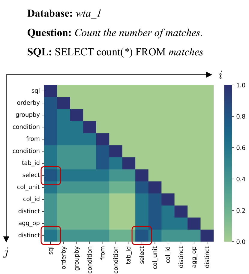
(a) Heatmap matrix of golden labels calculated by Eq.(4).

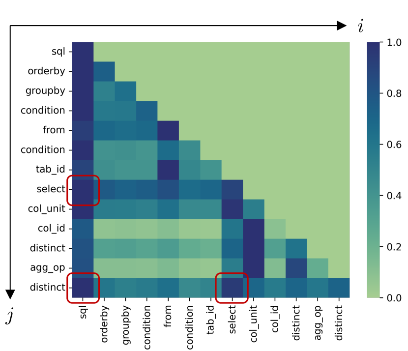
(b) Heatmap matrix of model predictions.

Figure 5: Visualization of target-side self-attention matrix among AST nodes.

In this part, we visualize the heatmap matrix of target-side self-attention in Figure 5. Assume that the relation between node $n_{j}$ and $n_{i}$ is $z_{ji}=(s,k)$, each entry with position $(j,i)$ in the golden heatmap matrix is computed via

$$\text{score}(j,i)=1-\frac{s+k}{2M},$$ (4)

where $M$ denotes the maximum depth of the current AST. In this way, we get an approximate scalar measure of the relative distance between any node pair. As for model predictions, we retrieve and take average of attention matrices $\alpha_{ji}^{h}$ from different heads $h$ in the last decoder layer. By comparison, we can find that: 1) The predicted attention matrix is highly similar to the golden reference based on path length. 2) Although some child/grandchild nodes are expanded in the distant future, they are still more correlated with their parent/grandparent, e.g., sql$\rightarrow$select$\rightarrow$distinct in Figure 5.

References

- Ba et al. (2016) Jimmy Lei Ba, Jamie Ryan Kiros, and Geoffrey E Hinton. 2016. Layer normalization. arXiv preprint arXiv:1607.06450.
- Bender et al. (2005) Michael A Bender, Martin Farach-Colton, Giridhar Pemmasani, Steven Skiena, and Pavel Sumazin. 2005. Lowest common ancestors in trees and directed acyclic graphs. Journal of Algorithms, 57(2):75–94.
- Cai and Wan (2020) Yitao Cai and Xiaojun Wan. 2020. IGSQL: Database schema interaction graph based neural model for context-dependent text-to-SQL generation. In Proceedings of the 2020 Conference on Empirical Methods in Natural Language Processing (EMNLP), pages 6903–6912, Online. Association for Computational Linguistics.
- Cao et al. (2021) Ruisheng Cao, Lu Chen, Zhi Chen, Yanbin Zhao, Su Zhu, and Kai Yu. 2021. LGESQL: Line graph enhanced text-to-SQL model with mixed local and non-local relations. In Proceedings of the 59th Annual Meeting of the Association for Computational Linguistics and the 11th International Joint Conference on Natural Language Processing (Volume 1: Long Papers), pages 2541–2555, Online. Association for Computational Linguistics.
- Cho et al. (2014) Kyunghyun Cho, Bart van Merriënboer, Caglar Gulcehre, Dzmitry Bahdanau, Fethi Bougares, Holger Schwenk, and Yoshua Bengio. 2014. Learning phrase representations using RNN encoder–decoder for statistical machine translation. In Proceedings of the 2014 Conference on Empirical Methods in Natural Language Processing (EMNLP), pages 1724–1734, Doha, Qatar. Association for Computational Linguistics.
- Clark et al. (2020) Kevin Clark, Minh-Thang Luong, Quoc V. Le, and Christopher D. Manning. 2020. ELECTRA: pre-training text encoders as discriminators rather than generators. In 8th International Conference on Learning Representations, ICLR 2020, Addis Ababa, Ethiopia, April 26-30, 2020. OpenReview.net.
- Cui et al. (2019) Yiming Cui, Wanxiang Che, Ting Liu, Bing Qin, Ziqing Yang, Shijin Wang, and Guoping Hu. 2019. Pre-training with whole word masking for chinese bert. arXiv preprint arXiv:1906.08101.
- Devlin et al. (2019) Jacob Devlin, Ming-Wei Chang, Kenton Lee, and Kristina Toutanova. 2019. BERT: Pre-training of deep bidirectional transformers for language understanding. In Proceedings of the 2019 Conference of the North American Chapter of the Association for Computational Linguistics: Human Language Technologies, Volume 1 (Long and Short Papers), pages 4171–4186, Minneapolis, Minnesota. Association for Computational Linguistics.
- Dou et al. (2022) Longxu Dou, Yan Gao, Mingyang Pan, Dingzirui Wang, Jian-Guang Lou, Wanxiang Che, and Dechen Zhan. 2022. Unisar: A unified structure-aware autoregressive language model for text-to-sql. arXiv e-prints, pages arXiv–2203.
- Guo et al. (2021) Jiaqi Guo, Ziliang Si, Yu Wang, Qian Liu, Ming Fan, Jian-Guang Lou, Zijiang Yang, and Ting Liu. 2021. Chase: A large-scale and pragmatic chinese dataset for cross-database context-dependent text-to-sql. In Proceedings of the 59th Annual Meeting of the Association for Computational Linguistics and the 11th International Joint Conference on Natural Language Processing, pages 2316–2331, Online. Association for Computational Linguistics.
- Guo et al. (2019) Jiaqi Guo, Zecheng Zhan, Yan Gao, Yan Xiao, Jian-Guang Lou, Ting Liu, and Dongmei Zhang. 2019. Towards complex text-to-SQL in cross-domain database with intermediate representation. In Proceedings of the 57th Annual Meeting of the Association for Computational Linguistics, pages 4524–4535, Florence, Italy. Association for Computational Linguistics.
- Hochreiter and Schmidhuber (1997) Sepp Hochreiter and Jürgen Schmidhuber. 1997. Long short-term memory. Neural computation, 9(8):1735–1780.
- Hui et al. (2021) Binyuan Hui, Ruiying Geng, Qiyu Ren, Binhua Li, Yongbin Li, Jian Sun, Fei Huang, Luo Si, Pengfei Zhu, and Xiaodan Zhu. 2021. Dynamic hybrid relation exploration network for cross-domain context-dependent semantic parsing. In Proceedings of the AAAI Conference on Artificial Intelligence, volume 35, pages 13116–13124.
- Krishnamurthy et al. (2017) Jayant Krishnamurthy, Pradeep Dasigi, and Matt Gardner. 2017. Neural semantic parsing with type constraints for semi-structured tables. In Proceedings of the 2017 Conference on Empirical Methods in Natural Language Processing, pages 1516–1526, Copenhagen, Denmark. Association for Computational Linguistics.
- Lewis et al. (2020) Mike Lewis, Yinhan Liu, Naman Goyal, Marjan Ghazvininejad, Abdelrahman Mohamed, Omer Levy, Veselin Stoyanov, and Luke Zettlemoyer. 2020. Bart: Denoising sequence-to-sequence pre-training for natural language generation, translation, and comprehension. In Proceedings of the 58th Annual Meeting of the Association for Computational Linguistics, pages 7871–7880.
- Lin et al. (2020) Xi Victoria Lin, Richard Socher, and Caiming Xiong. 2020. Bridging textual and tabular data for cross-domain text-to-SQL semantic parsing. In Findings of the Association for Computational Linguistics: EMNLP 2020, pages 4870–4888, Online. Association for Computational Linguistics.
- Loshchilov and Hutter (2019) Ilya Loshchilov and Frank Hutter. 2019. Decoupled weight decay regularization. In 7th International Conference on Learning Representations, ICLR 2019, New Orleans, LA, USA, May 6-9, 2019. OpenReview.net.
- Ouyang et al. (2022) Long Ouyang, Jeff Wu, Xu Jiang, Diogo Almeida, Carroll L. Wainwright, Pamela Mishkin, Chong Zhang, Sandhini Agarwal, Katarina Slama, Alex Ray, John Schulman, Jacob Hilton, Fraser Kelton, Luke Miller, Maddie Simens, Amanda Askell, Peter Welinder, Paul Christiano, Jan Leike, and Ryan Lowe. 2022. Training language models to follow instructions with human feedback.
- Paszke et al. (2019) Adam Paszke, Sam Gross, Francisco Massa, Adam Lerer, James Bradbury, Gregory Chanan, Trevor Killeen, Zeming Lin, Natalia Gimelshein, Luca Antiga, Alban Desmaison, Andreas Köpf, Edward Yang, Zachary DeVito, Martin Raison, Alykhan Tejani, Sasank Chilamkurthy, Benoit Steiner, Lu Fang, Junjie Bai, and Soumith Chintala. 2019. Pytorch: An imperative style, high-performance deep learning library. In Advances in Neural Information Processing Systems 32: Annual Conference on Neural Information Processing Systems 2019, NeurIPS 2019, December 8-14, 2019, Vancouver, BC, Canada, pages 8024–8035.
- Peng et al. (2021) Han Peng, Ge Li, Wenhan Wang, Yunfei Zhao, and Zhi Jin. 2021. Integrating tree path in transformer for code representation. Advances in Neural Information Processing Systems, 34:9343–9354.
- Qi et al. (2022) Jiexing Qi, Jingyao Tang, Ziwei He, Xiangpeng Wan, Chenghu Zhou, Xinbing Wang, Quanshi Zhang, and Zhouhan Lin. 2022. Rasat: Integrating relational structures into pretrained seq2seq model for text-to-sql. arXiv e-prints, pages arXiv–2205.
- Rabinovich et al. (2017) Maxim Rabinovich, Mitchell Stern, and Dan Klein. 2017. Abstract syntax networks for code generation and semantic parsing. In Proceedings of the 55th Annual Meeting of the Association for Computational Linguistics (Volume 1: Long Papers), pages 1139–1149.
- Raffel et al. (2020) Colin Raffel, Noam Shazeer, Adam Roberts, Katherine Lee, Sharan Narang, Michael Matena, Yanqi Zhou, Wei Li, and Peter J Liu. 2020. Exploring the limits of transfer learning with a unified text-to-text transformer. Journal of Machine Learning Research, 21:1–67.
- Rubin and Berant (2021) Ohad Rubin and Jonathan Berant. 2021. Smbop: Semi-autoregressive bottom-up semantic parsing. In Proceedings of the 5th Workshop on Structured Prediction for NLP (SPNLP 2021), pages 12–21.
- Scholak et al. (2021a) Torsten Scholak, Raymond Li, Dzmitry Bahdanau, Harm de Vries, and Christopher Pal. 2021a. Duorat: Towards simpler text-to-sql models. In Proceedings of the 2021 Conference of the North American Chapter of the Association for Computational Linguistics: Human Language Technologies, pages 1313–1321.
- Scholak et al. (2021b) Torsten Scholak, Nathan Schucher, and Dzmitry Bahdanau. 2021b. PICARD: Parsing incrementally for constrained auto-regressive decoding from language models. In Proceedings of the 2021 Conference on Empirical Methods in Natural Language Processing, pages 9895–9901, Online and Punta Cana, Dominican Republic. Association for Computational Linguistics.
- See et al. (2017) Abigail See, Peter J. Liu, and Christopher D. Manning. 2017. Get to the point: Summarization with pointer-generator networks. In Proceedings of the 55th Annual Meeting of the Association for Computational Linguistics (Volume 1: Long Papers), pages 1073–1083, Vancouver, Canada. Association for Computational Linguistics.
- Shaw et al. (2018) Peter Shaw, Jakob Uszkoreit, and Ashish Vaswani. 2018. Self-attention with relative position representations. In Proceedings of the 2018 Conference of the North American Chapter of the Association for Computational Linguistics: Human Language Technologies, Volume 2 (Short Papers), pages 464–468, New Orleans, Louisiana. Association for Computational Linguistics.
- Sun et al. (2020) Zeyu Sun, Qihao Zhu, Yingfei Xiong, Yican Sun, Lili Mou, and Lu Zhang. 2020. Treegen: A tree-based transformer architecture for code generation. In Proceedings of the AAAI Conference on Artificial Intelligence, volume 34, pages 8984–8991.
- Tipirneni et al. (2022) Sindhu Tipirneni, Ming Zhu, and Chandan K Reddy. 2022. Structcoder: Structure-aware transformer for code generation. arXiv e-prints, pages arXiv–2206.
- Vaswani et al. (2017) Ashish Vaswani, Noam Shazeer, Niki Parmar, Jakob Uszkoreit, Llion Jones, Aidan N Gomez, Łukasz Kaiser, and Illia Polosukhin. 2017. Attention is all you need. In Advances in neural information processing systems, pages 5998–6008.
- Wang et al. (2020a) Bailin Wang, Richard Shin, Xiaodong Liu, Oleksandr Polozov, and Matthew Richardson. 2020a. RAT-SQL: Relation-aware schema encoding and linking for text-to-SQL parsers. In Proceedings of the 58th Annual Meeting of the Association for Computational Linguistics, pages 7567–7578, Online. Association for Computational Linguistics.
- Wang et al. (2018) Chenglong Wang, Po-Sen Huang, Alex Polozov, Marc Brockschmidt, and Rishabh Singh. 2018. Execution-guided neural program decoding. CoRR, abs/1807.03100.
- Wang et al. (1997) Daniel C Wang, Andrew W Appel, Jeffrey L Korn, and Christopher S Serra. 1997. The zephyr abstract syntax description language. In DSL, volume 97, pages 17–17.
- Wang et al. (2020b) Lijie Wang, Ao Zhang, Kun Wu, Ke Sun, Zhenghua Li, Hua Wu, Min Zhang, and Haifeng Wang. 2020b. DuSQL: A large-scale and pragmatic Chinese text-to-SQL dataset. In Proceedings of the 2020 Conference on Empirical Methods in Natural Language Processing (EMNLP), pages 6923–6935, Online. Association for Computational Linguistics.
- Wolf et al. (2020) Thomas Wolf, Lysandre Debut, Victor Sanh, Julien Chaumond, Clement Delangue, Anthony Moi, Pierric Cistac, Tim Rault, Rémi Louf, Morgan Funtowicz, Joe Davison, Sam Shleifer, Patrick von Platen, Clara Ma, Yacine Jernite, Julien Plu, Canwen Xu, Teven Le Scao, Sylvain Gugger, Mariama Drame, Quentin Lhoest, and Alexander M. Rush. 2020. Transformers: State-of-the-art natural language processing. In Proceedings of the 2020 Conference on Empirical Methods in Natural Language Processing: System Demonstrations, pages 38–45, Online. Association for Computational Linguistics.
- Xie et al. (2022) Tianbao Xie, Chen Henry Wu, Peng Shi, Ruiqi Zhong, Torsten Scholak, Michihiro Yasunaga, Chien-Sheng Wu, Ming Zhong, Pengcheng Yin, Sida I Wang, et al. 2022. Unifiedskg: Unifying and multi-tasking structured knowledge grounding with text-to-text language models. arXiv preprint arXiv:2201.05966.
- Yin and Neubig (2017) Pengcheng Yin and Graham Neubig. 2017. A syntactic neural model for general-purpose code generation. In Proceedings of the 55th Annual Meeting of the Association for Computational Linguistics (Volume 1: Long Papers), pages 440–450, Vancouver, Canada. Association for Computational Linguistics.
- Yin and Neubig (2018) Pengcheng Yin and Graham Neubig. 2018. TRANX: A transition-based neural abstract syntax parser for semantic parsing and code generation. In Proceedings of the 2018 Conference on Empirical Methods in Natural Language Processing: System Demonstrations, pages 7–12, Brussels, Belgium. Association for Computational Linguistics.
- Yu et al. (2020a) Tao Yu, Chien-Sheng Wu, Xi Victoria Lin, Yi Chern Tan, Xinyi Yang, Dragomir Radev, Caiming Xiong, et al. 2020a. Grappa: Grammar-augmented pre-training for table semantic parsing. In International Conference on Learning Representations.
- Yu et al. (2018a) Tao Yu, Michihiro Yasunaga, Kai Yang, Rui Zhang, Dongxu Wang, Zifan Li, and Dragomir Radev. 2018a. Syntaxsqlnet: Syntax tree networks for complex and cross-domain text-to-sql task. In Proceedings of the 2018 Conference on Empirical Methods in Natural Language Processing, pages 1653–1663.
- Yu et al. (2019a) Tao Yu, Rui Zhang, Heyang Er, Suyi Li, Eric Xue, Bo Pang, Xi Victoria Lin, Yi Chern Tan, Tianze Shi, Zihan Li, Youxuan Jiang, Michihiro Yasunaga, Sungrok Shim, Tao Chen, Alexander Fabbri, Zifan Li, Luyao Chen, Yuwen Zhang, Shreya Dixit, Vincent Zhang, Caiming Xiong, Richard Socher, Walter Lasecki, and Dragomir Radev. 2019a. CoSQL: A conversational text-to-SQL challenge towards cross-domain natural language interfaces to databases. In Proceedings of the 2019 Conference on Empirical Methods in Natural Language Processing and the 9th International Joint Conference on Natural Language Processing (EMNLP-IJCNLP), pages 1962–1979, Hong Kong, China. Association for Computational Linguistics.
- Yu et al. (2020b) Tao Yu, Rui Zhang, Alex Polozov, Christopher Meek, and Ahmed Hassan Awadallah. 2020b. Score: Pre-training for context representation in conversational semantic parsing. In International Conference on Learning Representations.
- Yu et al. (2018b) Tao Yu, Rui Zhang, Kai Yang, Michihiro Yasunaga, Dongxu Wang, Zifan Li, James Ma, Irene Li, Qingning Yao, Shanelle Roman, Zilin Zhang, and Dragomir Radev. 2018b. Spider: A large-scale human-labeled dataset for complex and cross-domain semantic parsing and text-to-SQL task. In Proceedings of the 2018 Conference on Empirical Methods in Natural Language Processing, pages 3911–3921, Brussels, Belgium. Association for Computational Linguistics.
- Yu et al. (2019b) Tao Yu, Rui Zhang, Michihiro Yasunaga, Yi Chern Tan, Xi Victoria Lin, Suyi Li, Heyang Er, Irene Li, Bo Pang, Tao Chen, Emily Ji, Shreya Dixit, David Proctor, Sungrok Shim, Jonathan Kraft, Vincent Zhang, Caiming Xiong, Richard Socher, and Dragomir Radev. 2019b. SParC: Cross-domain semantic parsing in context. In Proceedings of the 57th Annual Meeting of the Association for Computational Linguistics, pages 4511–4523, Florence, Italy. Association for Computational Linguistics.
- Zhang et al. (2019) Rui Zhang, Tao Yu, Heyang Er, Sungrok Shim, Eric Xue, Xi Victoria Lin, Tianze Shi, Caiming Xiong, Richard Socher, and Dragomir Radev. 2019. Editing-based SQL query generation for cross-domain context-dependent questions. In Proceedings of the 2019 Conference on Empirical Methods in Natural Language Processing and the 9th International Joint Conference on Natural Language Processing (EMNLP-IJCNLP), pages 5338–5349, Hong Kong, China. Association for Computational Linguistics.
- Zheng et al. (2022) Yanzhao Zheng, Haibin Wang, Baohua Dong, Xingjun Wang, and Changshan Li. 2022. Hie-sql: History information enhanced network for context-dependent text-to-sql semantic parsing. In Findings of the Association for Computational Linguistics: ACL 2022, pages 2997–3007.
- Zhong et al. (2020a) Ruiqi Zhong, Tao Yu, and Dan Klein. 2020a. Semantic evaluation for text-to-SQL with distilled test suites. In Proceedings of the 2020 Conference on Empirical Methods in Natural Language Processing (EMNLP), pages 396–411, Online. Association for Computational Linguistics.
- Zhong et al. (2020b) Victor Zhong, Mike Lewis, Sida I Wang, and Luke Zettlemoyer. 2020b. Grounded adaptation for zero-shot executable semantic parsing. In Proceedings of the 2020 Conference on Empirical Methods in Natural Language Processing (EMNLP), pages 6869–6882.
- Zhong et al. (2017) Victor Zhong, Caiming Xiong, and Richard Socher. 2017. Seq2sql: Generating structured queries from natural language using reinforcement learning. CoRR, abs/1709.00103.