Small Language Models Fine-tuned to Coordinate Larger Language Models improve Complex Reasoning

Abstract

Large Language Models (LLMs) prompted to generate chain-of-thought (CoT) exhibit impressive reasoning capabilities. Recent attempts at prompt decomposition toward solving complex, multi-step reasoning problems depend on the ability of the LLM to simultaneously decompose and solve the problem. A significant disadvantage is that foundational LLMs are typically not available for fine-tuning, making adaptation computationally prohibitive. We believe (and demonstrate) that problem decomposition and solution generation are distinct capabilites, better addressed in separate modules, than by one monolithic LLM. We introduce DaSLaM, which uses a decomposition generator to decompose complex problems into subproblems that require fewer reasoning steps. These subproblems are answered by a solver. We use a relatively small (13B parameters) LM as the decomposition generator, which we train using policy gradient optimization to interact with a solver LM (regarded as black-box) and guide it through subproblems, thereby rendering our method solver-agnostic. Evaluation on multiple different reasoning datasets reveal that with our method, a 175 billion parameter LM (text-davinci-003) can produce competitive or even better performance, compared to its orders-of-magnitude larger successor, GPT-4. Additionally, we show that DaSLaM is not limited by the solver’s capabilities as a function of scale; e.g., solver LMs with diverse sizes give significant performance improvement with our solver-agnostic decomposition technique. Exhaustive ablation studies evince the superiority of our modular finetuning technique over exorbitantly large decomposer LLMs, based on prompting alone.

1 Introduction

In recent years, an astounding variety of text and NLP tasks have been accomplished by language models (LMs) Devlin et al. (2019) — in essence, fitting continuous feature vectors to tokens and modeling smooth conditional distributions over thousands of token positions with multi-task objectives. The next generation of large LMs (LLMs) such as T5, GPT4 and Bard (Raffel et al., 2020; OpenAI, 2023) developed protean capabilities, extending to mathematical and logical ability, based on prompting and in-context learning. Chain-of-thought (CoT) prompting has been a key enabler (Wei et al., 2022; Feng et al., 2023). LLMs can solve middle-school word problems and equations reasonably well. It has also acquired the ability to invoke specialized external tools such as Wolfram Alpha Wolfram (2023); Schick et al. (2023).

Recent advances in LLMs have arisen largely from cleverly-engineered, ever-growing training data, rather than any significant change in network structure, which remains relatively regular, but with rapidly increasing network size and number of parameters. One outcome of such giant monolithic LLMs is unsustainable levels of hardware and energy Dhar (2020) to train them. Meanwhile, neurologists and brain scientists have known, via fMRI scans, inter alia, that cerebral functions are specialized and spatially localized Fedorenko and Varley (2016); Mahowald et al. (2023).

Many recent complex reasoning challenges thrown at LLMs have a two-level character – the input task needs to be decomposed into subtasks, then the subtasks need to be solved, and finally, subtask solutions have to be consolidated and combined to solve the input task. Existing approaches use the same LLM to both decompose and solve the task, sometimes in tangled and uninterpretable ways. Because the sharing of an LLM across these functions cannot be closely controlled, very large models are needed for this double ability (decompose and solve) to emerge.

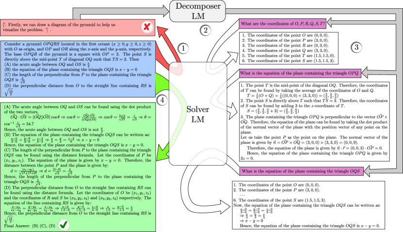
Figure 1: Working example of DaSLaM on a mathematical reasoning question from the JEEBench dataset (Arora et al., 2023). In this example, the solver LM is text-davinci-003. In step , the solver is prompted to answer the question ( blue textbox) and it fails to answer correctly ( red textbox). A problem decomposing LM generates subproblems ( violet textboxes) conditioned on the original question and the initial response of the solver in step . In step , the solver answers these subproblems iteratively and appends to the prompt. Finally, the original problem is appended to the prompt in step , and the solver answers it correctly ( green textbox).

Staying entirely inside the LLM regime, and avoiding the possibility of specialized tools, we ask a simple question – is it possible to offload the ability of problem decomposition to a dedicated, relatively smaller scale model, which is specialized and can act in synergy with any solver model of choice? To incorporate flexibility and better generalization, an immediate requirement of such a setup would be to enable a model-agnostic communication between the decomposer and the solver.

Our contributions.

To study this research question, we develop DaSLaM (Decomposition And Solution LAnguage Models), in which we separate the decomposer from the solver, as shown in Figure 1. The solver LM can be conventionally trained or fine-tuned. In the illustration, when it answers a question incorrectly, the decomposer LM takes over to produce sub-questions. The partial solutions are appended and resubmitted to the solver LM, which solves the question correctly. The decomposer LM regards the solver as a black box, and uses reinforcement learning (RL) to become a specialized expert at decomposition, informed by the solver’s mistakes.

Extensive experiments with three reasoning datasets (MATH, AQuA, and JEEBench) show that the proposed specialization improves the performance of OpenAI GPT-3 text-davinci-003 to outperform GPT-3.5 and even begins to compete with GPT-4, outperforming other similar methods. DaSLaM boosts text-davinci-003 from an exact match accuracy of $41.6$ to $54.5$ in zero-shot regime, which is $3.9$ points higher than few-shot GPT-4. Similarly, on Physics problems from JEEBench dataset, DaSLaM-augmented text-davinci-003 scores only $0.58$ points short of GPT-4 while outperforming GPT-3.5. The decomposer LM in DaSLaM reduces decomposition errors, and generalizes well across diverse small-scale LMs. It is also more robust in the face of difficult datasets, where the solver gives near-random performance.

These results support our founding hypothesis that heterogeneous functional specialization improves model efficiency and robustness of LLMs. A crucial findings from our experiments is that finetuning the decomposer is much more powerful choice than finetuning the solver. Moreover, a finetuned decomposer is largely superior compared to an orders of magnitude larger LLM prompted to act as a decomposer. Given the prohibitive cost of finetuning LLMs like GPT 3, 3.5, or 4, we hope this method would provide us a promising direction towards future development of task-expert models.

2 Related Work

Eliciting superior reasoning abilities in LM through specially designed prompts has found its popularity through CoT prompting Wei et al. (2022) – asking the LM to explain the reasoning steps improves overall performance. Decomposing a complex reasoning requirement into multiple, simple steps results in superior reasoning capabilities across modalities other than free-form natural language text as well, e.g., reasoning over tabular data (Ye et al., 2023), visual question answering Lu et al. (2022), etc. These methods generally solicit a single run of LM inference with no intermediate prompting interactions. Consequently, the LM often misses key reasoning steps or hallucinates irrelevant ones.

On the other hand, a prototypical prompter, sequentially interacting with the LM, has shown impressive performance. Progressive Hint Prompting Zheng et al. (2023) uses such a setting; first, the LM is asked to provide a base answer. The prompt then uses the answer as a hint to the LM that progressively guides it to the final answer. Zhou et al. (2023) followed a similar direction by breaking down the problem itself. Their method, Least-to-most prompting, asks the LM to generate simpler, related problems from a complex problem. The final solution to the original question is generated by the LM conditioned upon the solution of the subproblems. A major bottleneck then becomes the solver’s ability to identify the critical subproblems. Decomposing a complex task and then solving each task via multiple LLMs with their own in-context examples have been attempted as well (Dua et al., 2022; Khot et al., 2023). Recently, Shridhar et al. (2022) explored subquestion generation from complex questions as means of distilling reasoning abilities from larger LMs to smaller ones.

Our proposed method, DaSLaM makes a departure from these mentioned approaches in three particular features: (i) we seek to separate out the decomposer from the solver to get rid of the solver’s limitations affecting decomposition, (ii) the decomposer acts as a plug-and-play module that can generalize to any solver, and (iii) the decomposition actuates with complete knowledge of the solver’s actions.

3 A General Overview of DaSLaM

Given an LM $\theta$ and a question $Q$ as a sequence of tokens, a standard zero-shot prompting can be described as,

$$\hat{A}=\operatorname*{arg\,max}_{A\in\mathcal{A}}p_{\theta}(A|Q)$$

where $\hat{A}$ is the inferred answer, and $\mathcal{A}$ is the set of possible answers (e.g., numerical values, multiple-choice options, True/False, etc.). With a CoT prompting, the LM generates a sequence of tokens explaining the steps $S$ to reach the answer given the question. The modified process can be described as,

$$\hat{A}=\operatorname*{arg\,max}_{A\in\mathcal{A}}\left[p_{\theta}(A|S,Q)\operatorname*{arg\,max}_{S}p_{\theta}(S|Q)\right]$$ (1)

When answering $Q$ requires multistep reasoning, one can conceptualize $S$ as a sequence of smaller steps $\{S^{\prime}_{1},S^{\prime}_{2},\cdots,S^{\prime}_{n}\}$ such that the LM iteratively answers a sequence of subproblems $\{Q^{\prime}_{1},\cdots,Q^{\prime}_{n}\}$ to finally reach the desired answer to the original question. Eq. 1 can then be rewritten as,

$$\hat{A}=\operatorname*{arg\,max}_{A^{\prime}_{n}\in\mathcal{A}}\prod_{i}p_{\theta}(A^{\prime}_{i}|S^{\prime}_{i},Q^{\prime}_{i})\operatorname*{arg\,max}_{S^{\prime}_{i}}p_{\theta}(S^{\prime}_{i}|Q^{\prime}_{i})$$ (2)

where $A^{\prime}_{i}$ is the answer to the subproblem $Q^{\prime}_{i}$. In the usual regime of CoT, the subproblems $Q^{\prime}_{i}$ are implicit; the LM discovers them on its own and generates the reasoning steps and the answers. Due to the repeated multiplication in Eq. 2, any error in the initial stages quickly propagates along the chain of steps.

In DaSLaM, we seek to alleviate this problem by offloading the task of inferring the subproblems $\{Q^{\prime}_{i}\}$ to a decomposer LM $\phi$. For a more guided problem decomposition, DaSLaM uses the answer and the steps generated by the solver LM, $\theta$ in the naive CoT regime as described in Eq. 1 to generate a set of subproblems $\{\hat{Q}_{i}\}_{i=1,\ldots,n}$ as follows:

$$\hat{Q}_{i}=\operatorname*{arg\,max}_{Q^{\prime}_{i}}p_{\phi}(Q^{\prime}_{i}| \{\hat{Q}_{j}:j\in[1,i-1]\},$$

$$Q,\hat{A}_{0},S_{0}),$$ (3)

for $i\in[1,n]$, where $\hat{A}_{0}$ and $S_{0}$ are the initial answer and reasoning steps, respectively generated by $\theta$. The solver LM $\theta$ then solves the subproblem set one-by-one similar to Eq. 2. However, instead of seeking to generate the final answer as a response to the last subproblem $\hat{Q}_{n}$, we append the original question at the end and let $\theta$ answer it directly given the context generated by the subproblems, their answers, and the corresponding CoTs. The four stages of workflow with DaSLaM, as described in Figure 1, can then be summarized as follows:

$$\begin{split}&\hat{A}_{0}=\operatorname*{arg\,max}_{A\in\mathcal{A}}\left[p_{\theta}(A|S_{0},Q)\operatorname*{arg\,max}_{S_{0}}p_{\theta}(S_{0}|Q)\right]\\ &\hat{Q}_{i}=\operatorname*{arg\,max}_{Q^{\prime}_{i}}p_{\phi}(Q^{\prime}_{i}|\{\hat{Q}_{j}\}_{j\in\{1,i-1\}},Q,\hat{A}_{0},S_{0})\\ &\hat{A}_{i}=\operatorname*{arg\,max}_{A_{i}\in\mathcal{A}}\left[p_{\theta}(A_{i}|S_{i},\hat{Q}_{i})\operatorname*{arg\,max}_{S_{i}}p_{\theta}(S_{i}|\hat{Q}_{i})\right]\\ &\begin{split}\hat{A}=\operatorname*{arg\,max}_{A\in\mathcal{A}}\bigg{[}&p_{\theta}(A|S,Q)\\ &\operatorname*{arg\,max}_{S}p_{\theta}(S|\{\hat{A}_{i},S_{i},\hat{Q}_{i}\}_{i\in\{1,N\}},Q)\bigg{]}\end{split}\end{split}$$ (4)

4 Learning to Decompose from Feedback

Typical LMs are not suitable to reliably perform the problem decomposition stage in Eq. 3. We seek to finetune the decomposer LM, $\phi$ for this task. Specifically, we use the LLaMA 13 billion model. Instead of full LM-tuning, we use LoRA adapters (Hu et al., 2022) for parameter-efficient training. For brevity, we will denote the adapter-augmented LM as $\phi$, although only the adapter weights are being updated while training. The whole process of teaching the LM to perform the problem decomposition comprises two successive stages: (i) subproblem construction from the original question and CoT, and (ii) policy optimization in conjunction with the solver LM. Details of the supervised data curation required for these three steps are described in Section 5. Each data sample in the supervised dataset $\mathcal{D}$ can be conceptualized as a sequence of triplets $\langle Q_{\text{gold}},S_{\text{gold}},A_{\text{gold}},{\bf Q^{\prime}}_{\text{gold}}\rangle$, where $Q_{\text{gold}}$ denotes the original question, $S_{\text{gold}}$ denotes reasoning steps in form of CoT, $A_{\text{gold}}$ denotes the answer to the question, and ${\bf Q^{\prime}}_{\text{gold}}$ is a sequence of subproblems generated by decomposing $Q_{\text{gold}}$ (see Section 5 and Appendix A for further details on supervised data curation process).

The first stage is straightforward with the decomposer LM being finetuned using language modeling objective. In the first stage, we seek to optimize the following objective:

$$\min_{\phi}[-\log(p_{\phi}({\bf Q^{\prime}}_{\text{gold}}|Q,S))]$$ (5)

This step is somewhat similar to instruction tuning, where an LM is asked to generate some text conditioned on a context, instead of following the usual sentence completion-style behavior of the LM. Intuitively, the role of this stage is to align the LM to the task of the decomposer.

Decomposition via policy network.

The previous stage inculcates the ability to decompose a problem within $\phi$. However, it is still blind to the actual errors made by the solver LM. In the next stage, we seek to make the decomposer LM work in synergy with any solver LM of choice. This solver agnosticism restrains $\phi$ to observe the internal representations computed by $\theta$ while solving the problem. To handle this imposed blackbox characteristics of the solver, we resort to policy gradient optimization of $\phi$ assuming $\theta$ to be part of the environment. We formalize the setup as follows.

Elements of the environment: The solver LM $\theta$ constitutes the core component of the environment. Given a question $Q$, the solver-generated CoT $S$ and the answer $A$ as sequences of tokens define the observation of the policy.

State and action space: We define the state space as $\mathcal{S}$. The initial state, $s_{0}\in\mathcal{S}$, is defined by the original question $Q$ and the initial response from the solver, $S_{0},A_{0}$, that are provided to the decomposer LM $\phi$ as input. A single timestep is defined on generation of a single token, i.e., the action $a_{t}$ at time $t$. Given the autoregressive nature of LM, we define the state at $t$-th timestep as $s_{t}=(s_{t-1},\{a_{t-1}\})$, i.e., the token generated at $t-1$ appended to the tokens generated till $t-1$. Trivially, the action space is the same as $\mathcal{V}$, the vocabulary of $\phi$.

Policy: The decomposer LM is conceptualized as a policy network $\pi_{\phi}:\mathcal{S}\xrightarrow{}\mathcal{V}$, i.e., it generates a token given the inputs and the token generated hitherto, till the end of episode $T$. Inspired by the recent success in Reinforcement Learning from Human Feedback (RLHF) with autoregressive LMs, we choose the Proximal Policy Optimization (PPO) algorithm to train the policy $\pi_{\phi}(a|s)$. In a typical PPO setup, we define the advantage function as follows:

$$\hat{G}_{t}=\sum_{i=0}^{T-t+1}(\gamma\lambda)^{i}\left[r_{t+i}+\gamma V(s_{t+i+1})-V(s_{t+i})\right]$$ (6)

where $r_{t}$ is the reward at step $t$, $V(s_{t}):\mathcal{S}\xrightarrow{}\mathbb{R}$ is the value function determining the reward associated to state $s_{t}$, and $\gamma,\lambda$ are hyperparameters. We use the policy model augmented with a randomly initialized feedforward layer as the value function. A crucial component in on-policy learning regime is the reward function $r_{t}$. While the end goal of the learning is to have the solver answering correctly, the decomposer LM should receive some incremental signal aligned to its generation as well for it to stably converge to the optimal policy. With this goal in mind, we construct the reward function as,

$$r_{t}=R_{1}+R_{2}+R_{3}+R_{4}+R_{5}$$ (7)

where $R_{1}$ to $R_{5}$ are defined as follows (see Appendix B for a detailed treatment on the reward computation method). Here $\operatorname{cos-sim}$ represents cosine similarity. $I(x)=1$ if $x$ is true is the indicator function.

Entity coverage:

$R_{1}=\frac{|E_{\bf Q^{\prime}}|}{|E_{Q}|}$, where $E_{\bf Q^{\prime}}$ and $E_{Q}$ are the sets of distinct entities in the generated subproblems and the original question, respectively.

Consistency of answers to subproblems:

$$R_{2}=\sum_{i}\big{(}I({e_{i}}={\hat{e_{i}}})+\operatorname{cos-sim}(Q^{\prime}_{i},A_{i})\big{)}$$ (8)

where $\hat{e_{i}}$ is the entity whose value has been asked in the subproblem $Q^{\prime}_{i}$, and ${e_{i}}$ is the entity answered. This reward penalizes the decomposer LM for generating questions whose answers are not consistent.

Order of operations:

$R_{3}=\frac{l}{m}$, where $l$ is the number of operations matched in order between $S$ and $S_{\text{gold}}$, and $m$ is the total number of operations in $S_{\text{gold}}$.

CoT proximity:

To ensure that the distance of reasoning produced by the model after prompting $S$ to the gold reasoning $S_{gold}$ is less than the distance of reasoning produced without prompt $S_{0}$ to the gold reasoning steps $S_{gold}$, we design a reward based on the cosine similarity of each step of $S_{gold}$. We break $S$ and $S_{0}$ at new-line token to form reasoning steps. At each step $j$, we compute $c_{1j}=\operatorname{cos-sim}(S^{j},S_{gold}^{j})$ and $c_{2j}=\operatorname{cos-sim}(S_{0}^{j},S_{gold}^{j})$. The reward is

$$R_{4}=\sum_{j=0}^{m}I(c_{1j}>c_{2j})c_{1j}+I(c_{2j}>c_{1j})(-1-c_{2j}),$$ (9)

Correctness of final answer:

$R_{5}{=}I(\hat{A}{=}A_{\text{gold}})$.

Now, we can define the PPO objective as follows:

$$\max_{\phi}\left(\mathbb{E}_{t}\left[\frac{\pi_{\phi}(a_{t}|s_{t})}{\pi_{\text{ref}}(a_{t}|s_{t})}\hat{G}_{t}\right]-\beta\mathbb{E}_{t}\left[K_{t}\right]\right)$$ (10)

where $\pi_{\text{ref}}$ is the reference model that is initialized with supervised finetuned $\phi$. $K_{t}=\operatorname{KL}[\pi_{\text{ref}}(\cdot|s_{t}),\pi_{\phi}(\cdot|s_{t})]$ is the KL-divergence between the reference model and the policy model.

The resulting decomposer LM $\phi$ optimized using the above mentioned three stages of finetuning can then be used with DaSLaM.

5 Experiments

Training data curation.

The training process of DaSLaM consists of two stages as mentioned previously. In the first stage, we require the subproblems along with the reasoning steps for a given problem. We use samples from four existing datasets — MATH Hendrycks et al. (2021), AQuA Ling et al. (2017), GSM8K Cobbe et al. (2021), and StrategyQA Geva et al. (2021). Each question in these four datasets contains a question $Q_{\text{gold}}$, a step-by-step illustration of the reasoning process $S_{\text{gold}}$, and the final answer $A_{\text{gold}}$. We sample $7,000$ examples from the training splits of these datasets and employ OpenAI’s text-davinci-003 model to generate the corresponding subquestions. We provide the model with one-shot example illustrating how to decompose a question into subquestions based on the reasoning. In the second stage of training, we utilize the remaining training data from MATH and AQuA datasets to conduct the policy optimization since this step does not require any supervised examples of subproblems.

LMs used.

We use LLaMA 13 billion Touvron et al. (2023) as the decomposer LM. For the solver LM, we primarily use text-davinci-003 (henceforth, we denote it as GPT-3.5 for brevity). We also experiment with the LLaMA 13 bilion and LLaMA 33 billion models as solvers to test the model-agnostic generalizability of DaSLaM.

Baselines.

We compare DaSLaM with four existing methods of prompting: Chain-of-thought prompting (CoT) (Wei et al., 2022), Least-to-most prompting (L2M) (Zhou et al., 2023), Progressive Hint Prompting (PHP) (Zheng et al., 2023), and, Demonstrate-Search-Predict (DSP) (Khattab et al., 2022a). The original setting of PHP requires an 8-shot prompting; however, since all other methods including DaSLaM predict in the zero-shot setting, we use PHP in 1-shot for a fairer comparison. Additionally, we experiment with three ablation variants: DaSLaM-NF does not take the solver feedback into account while generating the subproblems; Finetuned is the solver LM (LLaMA 13B in this case, we could not finetune 33B variant due to computational constraints) finetuned without any decomposer; GPT-3.5 decomposer does away with the finetuned LLaMA 13B decomposer and uses pretrained GPT-3.5 as the prompted decomposer.

Dataset	Method
	CoT	L2M	PHP	DSP	GPT3.5 Decomposer	DaSLaM-NF	DaSLaM
PnC	$16.4$	$16.0$	$10.2$	$16.2$	$16.0$	$20.0$	$\bf 21.4$
NT	$14.4$	$11.0$	$9.8$	$20.3$	$14.2$	$18.4$	$\bf 26.1$
ALG	$27.6$	$22.4$	$24.0$	$15.3$	$32.1$	$31.6$	$\bf 33.4$
I-ALG	$16.4$	$16.8$	$10.0$	$17.0$	$18.4$	$20.8$	$\bf 24.8$
Calc.	$14.0$	$14.58$	$14.28$	$18.8$	$12.0$	$15.1$	$\bf 18.2$
P-ALG	$32.3$	$28.0$	$26.5$	$28.0$	$35.5$	$38.0$	$\bf 44.0$
Geom.	$14.2$	$12.5$	$14.0$	$5.2$	$\bf 22.0$	$19.04$	$21.4$
AQuA	$41.6$	$44.7$	$44.4$	$44.0$	$45.4$	$53.2$	$\bf 54.5$

Table 1: Performance comparison on MATH and AQuA datasets using GPT-3.5 as the solver LM. See Section 5 for abbreviations.

Test datasets.

For evaluation purposes, we use three datasets – MATH Hendrycks et al. (2021), AQuA (Ling et al., 2017), and JEEBench Arora et al. (2023). For the first two datasets, only the test splits are used during evaluation since their training splits are used while finetuning the decomposer. The MATH dataset contains mathematical problems on multiple different domains. We report the results on each of them separately and use the following abbreviations – ALG, I-ALG, and P-ALG for Algebra, Intermediate Algebra, and Pre-Algebra, respectively; Calc for Calculus, Geom for Geometry, PnC for Probability and Combinatorics, NT for Number theory. From the JEEBench dataset, we use the problems in Physics (Phy) and Mathematics (Math). Each of these two subjects has three types of problems – single-answer multiple-choice questions (MCQ), numerical problems (Num), and multi-answer multiple-choice questions (Multi). For all these datasets, we use exact match criteria to evaluate the correctness of the model-inferred answers. Details of training and inference hyperparameters and compute resource usage are provided in Appendix C.

6 Experimental Results

The tasks used to evaluate the performance of DaSLaM contain questions that can be answered either of the three types – numerical, single correct answer MCQ, and multiple correct answer MCQ.

Method	Dataset
	PnC	NT	ALG	iALG	Geom	Cal	Palg	AQuA
LLaMA 13 billion
CoT	2.05	4.0	3.12	2.4	3.2	2.08	5.0	17.7
L2M	1.66	3.2	3.33	2.8	2.0	3.33	4.54	16.6
Finetuned	2.8	3.6	3.57	3.2	4.1	3.05	6.04	19.4
GPT3.5 Decomposer	2.05	5.0	4.68	2.8	2.08	4.0	6.66	20.4
DaSLaM-NF	2.93	4.8	4.68	3.2	4.0	3.9	6.2	21.6
DaSLaM	4.0	5.6	4.70	3.4	4.3	4.1	8.33	22.0
LLaMA 33 billion
CoT	2.4	4.16	4.54	3.7	4.0	4.0	5.2	20.0
L2M	2.38	4.16	4.2	6.0	4.25	5.71	5.55	21.6
DaSLaM-NF	3.2	5.83	5.6	5.6	5.1	5.71	5.2	22.5
DaSLaM	4.0	7.36	9.09	6.02	5.3	6.03	8.44	26.8

Table 2: Performance on MATH and AQuA with LLaMA 13 billion and LLaMA 33 billion as solvers. PHP is not reported as one-shot PHP generated randomly with both LLaMA variants. DaSLaM provides consistent improvement across all the tasks while other baseline methods mostly fail.

Method	Dataset
	Phy MCQ	Math MCQ	Phy Multi	Math Multi	Phy Num	Math Num	Phy Int	Math Int
CoT	33.33	21.9	6.25	12.0	3.03	1.69	12.5	20.0
PHP	22.22	17.07	6.25	7.59	3.03	1.69	0*	4.0
L2M	22.22	21.9	6.25	12.5	3.03	3.38	10.0	20.0
DaSLaM-NF	20.8	31.7	7.5	10.12	3.03	3.38	12.5	16.0
DaSLaM	55.55	36.5	18.75	16.0	6.06	10.16	22.5	24.0
GPT-4	55.55	34.14	27.5	21.5	15.15	11.8	25.0	20.0

Table 3: Performance comparison on the JEE benchmark dataset with GPT-3.5 as the solver LM. 0* signifies that the model was not able to answer any problem in the task correctly.

DaSLaM is better than pure prompting We start with DaSLaM augmented with GPT-3.5 as the solver LM on MATH and AQuA datasets (see Table 1). The improvement achieved with DaSLaM prompting compared to standard CoT is staggering across all types of problems in the MATH dataset: $+11.7$ on Pre-Algebra, $+8.4$ on Intermediate Algebra, $+7.7$ on Number Theory, $+7.2$ on Geometry, $+5.0$ on Probability and Combinatorics, $+5.8$ on Algebra, and $+4.2$ on Calculus. The absolute improvement is even larger on the AQuA dataset, i.e., $+12.9$ over CoT. It is noticeable that the effects of DaSLaM are stronger across tasks containing algebraic reasoning (AQuA, Pre- and Intermediate-Algebra, etc.) compared to Probability and Combinatorics or Calculus, which require more implicit knowledge. The performance gain achieved via DaSLaM is significantly better compared to methods like L2M or PHP. The latter methods often fail to improve over standard CoT (e.g., on Probability and combinatorics, Number Theory, and Algebra problems, L2M shows a drop in accuracy). Even when improving over CoT, their improvement is meager compared to DaSLaM. This trend entails our earlier argument in support of offloading the problem decomposition task to a specialized LM; methods that prompt the solver LM to decompose the problem lack the expertise achieved via dedicated finetuning in DaSLaM.

Finetuned decomposer is essential. Despite being orders of magnitude smaller, a finetuned LLaMA 13B model delivers better performance compared to GPT-3.5 as a decomposer (DaSLaM vs. GPT-3.5 generator in Table 1 and 2). This further justifies our choice of separately finetuning the decomposer and the added flexibility that it offers. In fact, finetuning the decomposer is far effective compared to finetuning the solver (DaSLaM vs Finetuned solver in Table 2).

Feedback from the solver is important. In the preceding paragraph, we attributed the superiority of DaSLaM over other methods to the usage of a specialized LM for problem decomposition. However, manipulating the problem decomposition upon feedback from the solver is also an important factor here. None of the existing methods does so, and therefore, remains blind towards what reasoning (and possible errors) is followed by the solver model. This is further manifested when we compare DaSLaM with itself without the feedback module, DaSLaM-NF. While DaSLaM-NF is able to improve upon basic CoT and other prompting methods, it falls short of a decomposer LM that has access to the initial response of the solver.

DaSLaM generalizes to smaller solvers. An important aspect of a prompting method is its ability to work with LMs of different scales. Despite being finetuned with GPT-3.5 responses only, DaSLaM is able to improve upon the base performance of smaller scale LLaMA models as well (see Table 2). L2M prompting generally fails with both LLaMA 13 billion and 33 billion variants. On the other hand, DaSLaM, with or without feedback, almost doubles the performance of the base CoT across multiple tasks of the MATH dataset. It shows substantial improvement on AQuA as well. The importance of feedback from the solver LM usually manifests strongly in proportion to the scale of the solver.

DaSLaM generalizes to harder problems. Since the decomposer LM $\phi$ is trained using a subset of the training data of MATH and AQuA, we opt for a harder (in terms of benchmark performance of different LMs) reasoning evaluation on the JEEBench dataset. Table 3 summarizes the performance of the baselines and DaSLaM with GPT-3.5 as the solver LM on Mathematics and Physics questions of the JEEBench dataset. We notice that the superiority of DaSLaM manifests even more profoundly on this task compared to the former ones. Both PHP and L2M prompting absolutely fail to improve upon basic CoT prompting, often with a sharp fall in performance (e.g., Physics MCQ questions). On the other hand, DaSLaM boosts the LMs performance, very often over 100% relative improvement (all three types of problems in Physics and numerical problems in Mathematics). Aggregated across question types, DaSLaM boosts the performance of GPT-3.5 to $22.420$ in Physics and $22.07$ in Mathematics. It is noteworthy that the same LM in its base setting performs near-random, i.e., $10.4$ and $10.7$ in Physics and Mathematics, respectively, whereas a random selection baseline gives scores of $9.6$ and $10.3$, respectively (Arora et al., 2023). Furthermore, GPT-3.5 with DaSLaM outperforms a better optimized candidate of the GPT series, GPT-3.5 on both these subjects (note that Arora et al. (2023) reported $18.9$ and $15.7$ scores with GPT-3.5 on Physics and Mathematics, respectively).

Figure 2: An example case study on a problem from the MATH dataset. GPT-3.5 is used as the solver LM with three different methods of prompting – standard CoT, Least-to-most, and DaSLaM. Only DaSLaM is able to guide the model to the correct answer.

Comparison with GPT-4. The colossal compute used by GPT-4 makes the comparison with any of its predecessors like GPT-3.5 quite unfair. However, it is tempting to observe that DaSLaM boosts the performance of GPT-3.5 often to the level of GPT-4. For example, on arithmetic problems of the AQuA dataset, DaSLaM surprisingly outperforms both zero-shot and few-shot GPT-4 ($40.6$ and $50.4$ respectively, compared to $54.5$ with GPT-3.5 and DaSLaM). On MATH dataset, DaSLaM augmented GPT-3.5 scores an aggregate of $30.23$, which is better than ChatGPT ($26.4$) and close to GPT-4 ($35.7$). On JEEBench Mathematics problems, GPT-4 comes up with an aggregate score of $23.1$, which is pretty close to our $22.42$. In Physics and Math MCQ questions, DaSLaM with GPT-3.5 outperforms GPT-4. These results definitely do not claim any assumed superiority of DaSLaM-boosted GPT-3.5 over GPT-4 since there are multiple other cases that state otherwise. Instead, we seek to demonstrate how much leftover potential these LMs possess that can be unleashed via our proposed method of feedback-guided automatic problem decomposition.

7 Case Study

To this point, we have compared the numbers produced by DaSLaM-boosted models across different datasets. While they provide an overall assessment, deeper analyses are needed to comprehend the actual reasoning steps adopted by these different methods. Figure 2 shows the reasoning steps generated by GPT-3.5 given an example problem from the MATH dataset with three different prompting methods – vanilla CoT, L2M, and DaSLaM. Note that DaSLaM uses the CoT output to decompose the problem.

Both CoT and L2M end up with the model answering incorrectly. With CoT, the solver wrongly assumes that the given equation must have two real roots though it should not have any real roots. Also, it mistakes the value of $a^{2}$ as $a$. The effect is prominent in the subproblems generated by DaSLaM as it asks to find the value of $a$ explicitly. Furthermore, the solver LM specifically announces that $y\leq 0$ to answer the first subproblem generated by DaSLaM. This helps to correct the reasoning about the sign of the discriminant.

With L2M, the confusion around the value of $a$ and $a^{2}$ persists, as the solver LM substitutes $a$ in the given equation by $49$ (which is the value of $a^{2}$) twice in the answering process. Although it substituted the correct value of $a$ once while answering the second question, it is not explicitly declared like in DaSLaM. We observe multiple similar failure cases with L2M. It is quite likely that prompting the model to generate the final answer after each subproblem accumulates the erroneous reasoning steps that the model falls prey to.

With DaSLaM, the reasoning steps followed by the solver remains robust throughout. It reaches the final answer much earlier (third and fourth subproblems). In the final answer, the solver simply reiterates the steps that it earlier generated to answer the subproblems. This is a common behavior that we observed across multiple problems from multiple datasets. In Appendix D (see Figures 3 and 4), we provide similar case studies on LLaMA 13B and 33B with different prompting methods. With reduced solver capacity, the difference between Least-to-most and CoT generated reasoning steps further diminishes with both leading to incorrect answers; DaSLaM, on the other hand, still guides the solver through correct steps.

An interesting observation can be made by comparing how the solver behaves with CoT vs. with DaSLaM. With DaSLaM, we do not provide any new knowledge to the solver. Yet, the same model can rectify its errors made in CoT response. This may point to the intuition that current LLMs are actually underutilized, and one can unfold even more impressive performance with cleverly composed guidance.

We further provide case analyses with when DaSLaM fails to guide the model (GPT 3.5 in this case) to successful final answers, in Appendix E. While we do not find any obvious pattern of errors, one can see that the decomposer generates questions that are not readily answerable within that context. DaSLaM does not use any method to trace back the error or generate subproblems based on the answers to the previous subproblems. This might raise such issues where the subproblems generated are not actually helping the solver in the right order.

8 Conclusion

We challenged the design of ever-larger monolithic LLMs as homogeneous network structures, where diverse aspects of problem decomposition and solution are stored in a tangled and opaque manner. The formidable general-purpose problem-solving capabilities of LLMs are exceedingly resource-hungry, dependent on immense data engineering. Inspired by brain science, we took a first step toward heterogeneity — let two different LLMs evolve independently and adapt to their roles of decomposing and solving complex reasoning problems. Through extensive experiments on several benchmarks, we showed that such a heterogeneous network can match or exceed some of the largest contemporary LLMs, at a much smaller parameter count.

Limitations

A potential limitation of DaSLaM, as with many system that uses an LLM-as-a-service API charging per token exchange, is the increased token usage because of the RL exploration. Asserting a token budget on the decomposer LM is left as an avenue for future exploration. Ideally, the decomposer LM should seamlessly invoke solvers of many forms, such as retrievers (Khattab et al., 2022b) or mathematical calculators (Schick et al., 2023; Wolfram, 2023). Future work may extend DaSLaM to such tools. DaSLaM is limited to purely text-based subproblem decomposition; it is not possible at present to incorporate reasoning through other modalities (e.g., visual inputs for geometric reasoning) into DaSLaM in its current form.

Small Language Models Fine-tuned to Coordinate Larger Language Models improve Complex Reasoning
(Appendix)

Appendix A Supervised Fine-tuning Dataset

The training data for supervised fine-tuning stage was generated using text-davinci-003. Each data point in the dataset consisted of a tuple $\langle Q_{\text{gold}},S_{\text{gold}},{Q^{\prime}}_{\text{gold}}\rangle$, where $Q_{\text{gold}}$ represents the reasoning question, $S_{\text{gold}}$ represents the gold reasoning steps, and ${Q^{\prime}}_{\text{gold}}$ represent the sub-questions generated by text-davinci-003 in a one-shot setting. An example of a single data point is given below.

Appendix B Reward Calculation

During policy gradient optimization of the decomposer LM $\phi$, rewards were provided in an incremental fashion so that the generated sub-questions align well with the initial question, the answer generated by the solver LM $\theta$ and the sub-question solving capabilities of $\theta$. For this, the reward was designed as a combination of five terms. The definitions of these terms are given in Section 4. Here we provide an example of the reward calculation.

Entity coverage Reward ($R_{1}$). Here, we find distinct nouns and numbers in the question and the sub-questions using the nltk library. The reward is calculated using $R_{1}=\frac{|E_{\bf Q^{\prime}}|}{|E_{Q}|}$, where $E_{\bf Q^{\prime}}$ and $E_{Q}$ are the sets of distinct nouns and numbers in the sub-questions and questions, respectively. An example of the same is shown below.

Consistency of answers to subproblems reward ($R_{2}$). To ensure that the sub-question is such that the solver LLM $\phi$ does not produce random answers, we compare the entity in the solution to the entity asked in the subquestion along with the cosine similarity of the embeddings of sub-question and sub-answers. To find the embeddings, we use the pre-trained model in the spacy library. $R_{2}=\sum_{i}(I({e_{i}}={\hat{e_{i}}})+\operatorname{cosine-similarity}(Q^{\prime}_{i},A_{i}))$, where $I(x)=1$ if $x$ is true, $\hat{e_{i}}$ is entity whose value has been asked in the subproblem $Q^{\prime}_{i}$, and ${e_{i}}$ is the entity answered. An example for the reward calculation is given below.

Order of operations reward ($R_{3}$). To evaluate the correctness of the mathematical solution produced by the model, we compare the order of operations. $R_{3}=\frac{l}{m}$, where $l$ is the number of operations matched in order between $S$ and $S_{\text{gold}}$, and $m$ is the total number of operations in $S_{\text{gold}}$. Below is an example of $R_{3}$ calculation.

CoT Proximity reward ($R_{4}$). As defined in Section 4, $R_{4}=$$\sum_{j=0}^{m}I(c_{1j}>c_{2j})c_{1}+I(c_{2j}>c_{1j})(-1-c_{2j})$, where $I(\cdot)$ is the indicator function. Here we present an example to illustrate the same.

Correctness of final answer($R_{5})$, $R_{5}=I(\hat{A}=A_{\text{gold}})$. This reward checks if the final answer matches the gold answer. A negative example of the same is given below.

Appendix C Hyperparameter Selection

We performed hyperparameter tuning on a subset of 250 examples from the training dataset. Based on the improvement in accuracy and compute resources, we converged at the following values.

For the supervised fine-tuning stage, we used LoRA $r=16$, LoRA $\alpha$ = 32, LoRA droput = 0.05. For the RLMF stage, we finetuned the last 3 layers of LoRA adapters, using a batch size of 8, gradient accumulation steps=8, init kl coef=0.01, target=4. For inference, we used the following generation parameters: temperature = 0.95, top p=0.18, pad token id = 0, do sample = False, number of beams = 1, maxi length = 2048.

All the models were implemented using Huggingface with PyTorch, and loaded in int_8 precision. For solver-LLaMA 13B model, we instruction finetuned the LLaMA13B model using the Alpaca dataset by stanford  Taori et al. (2023). For solver-LLaMA 33 billion model, we used an instruction-finetuned version of LLAMA-33 billion from Huggingface. To implement the PPO algorithm, we used the TRL library. We used a single NVIDIA A100 (80GB) GPU for all training and inference purposes.

Appendix D Case Study on LLAMA Models

Similar to Figure 2, we performed example-wise case study on the answering process of the LLaMA solvers (13 billion and 33 billion models) with different prompting methods (see Figures 3 and 4). The example problem was selected from the MATH dataset. As we can see, with relatively small scale solvers like LLaMA, Least-to-most fails to add any improvement over basic CoT prompting. DaSLaM is able to guide the model to the correct answer in both cases.

Figure 3: A case study on LLAMA-13B.

Figure 4: A case study on LLaMA-33B as solver model.

Appendix E Failure cases with DaSLaM

E.1 Case I

Question A train running at a speed of 100 miles/hour, takes 10 hours to reach its destination. After covering quarter of the distance, it starts raining and the train has to be slowed to speed of 75 miles/hour. What is the total journey duration? A)10 B)11.5 C)12.5 D)13.5 E)15

Initial Answer The train covers the first quarter of the distance at a speed of 100 miles/hour.
So, the time taken to cover the first quarter of the distance = (1/4) x 10 hours = 2.5 hours
The train covers the remaining three quarters of the distance at a speed of 75 miles/hour.
So, the time taken to cover the remaining three quarters of the distance = (3/4) x 10 hours = 7.5 hours
Therefore, the total journey duration = 2.5 + 7.5 = 10 hours

Sub problem 1 What is the total distance to be covered?

Sub Answer 1 Let the total distance to be covered be d.
Time taken to cover the first quarter of the distance = (1/4)d/100 = 10/400 hours
Time taken to cover the remaining distance = (3/4)d/75 = 300/400 hours
Total time taken = 10/400 + 300/400 = 10/4 hours = 2.5 hours
Since the train takes 10 hours to reach its destination,
Total distance to be covered = 10 x 100 = 1000 miles

Sub problem 2
What is the speed of the train?

Sub Answer 2
After covering quarter of the distance, the train has to be slowed to speed of 75 miles/hour.

Let the remaining distance be x.

Therefore, x = d - (d/4) = 1000 - (1000/4) = 750 miles.

The time taken to cover the remaining distance x = 750 miles at a speed of 75 miles/hour = (750/75) hours = 10 hours.

Therefore, the speed of the train = x/time taken = 750/10 = 75 miles/hour.

Sub problem 3 What is the time taken to cover the distance?
Sub Answer 3
Time taken to cover the first quarter of the distance = (d/4)/100 hours = d/400 hours

Time taken to cover the remaining distance = (3d/4)/75 hours = d/300 hours

Total time taken = d/400 + d/300 = (5d + 4d)/1200 hours = 9d/1200 hours.

Putting d=1000,

Final answer: The time taken to cover the distance is 9 x 1000/1200 hours.

Sub problem 4 What is the total duration of the journey?
Sub Answer 4 Time taken to cover the first quarter of the distance = (d/4)/100 hours = d/400 hours

Time taken to cover the remaining three quarters of the distance = (3d/4)/75 hours = 4d/300 hours

Total time taken = d/400 + 4d/300 = (5d + 4d)/(400 + 300) = 9d/700 hours

Total duration of the journey = 9d/700 hours = 9 hours and (d/700) hours = 9 hours and (100/700) hours = 9 hours and 14.29 minutes

Final Answer Step 1: The train covers the first quarter of the journey at a speed of 100 miles/hour. Step 2: The time taken to cover the first quarter of the journey is given by: Time = Distance/Speed Time = (1/4) x 100/100 Time = 1/4 hour Step 3: The train covers the remaining three quarters of the journey at a speed of 75 miles/hour. Step 4: The time taken to cover the remaining three quarters of the journey is given by: Time = Distance/Speed Time = (3/4) x 75/100 Time = 3/4 hour Step 5: The total duration of the journey is the sum of the time taken to cover the first quarter and the remaining three quarters of the journey. Total Time = 1/4 + 3/4 Total Time = 4/4 Total Time = 1 hour Therefore, the total duration of the journey is 1 hour.

E.2 Case II

Question Consider there is an staircase elevator and you are coming down. If you walk 20 steps and stop, then you reach bottom in 10 minutes. If you walk 10 steps and stop, you reach to the ground in 20 minutes. What is the speed of the elevator? A)1 step/minute B)2 step/minute C)3 step/minute D)4 step/minute E)None of the above
Initial Answer .
Sub Question 1 What is the total number of steps in the elevator?
.
Sub Question 2 What is the speed of the elevator?
.
Sub Question 3
What is the time taken to cover 20 steps?
Sub Answer 3
Time taken to cover 20 steps is 10 minutes
Sub Question 4
What is the time taken to cover 10 steps?
Sub Answer 4
Time taken to cover 10 steps is 20 minutes
Final Answer Let the speed of the elevator be x. Time taken to reach the bottom when walking 20 steps and stopping = 10 minutes
Time taken to reach the bottom when walking 10 steps and stopping = 20 minutes
Therefore,
20x = 10
10x = 20
x = 2
Therefore, the speed of the elevator is 2 steps/minute.

E.3 Case III

Question Let $-\frac{\pi}{6}<\theta<-\frac{\pi}{12}$. Suppose $\alpha_{1}$ and $\beta_{1}$ are the roots of the equation $x^{2}-2x\sec\theta+1=0$ and $\alpha_{2}$ and $\beta_{2}$ are the roots of the equation $x^{2}+2x\tan\theta-1=0$. If $\alpha_{1}>\beta_{1}$ and $\alpha_{2}>\beta_{2}$, then $\alpha_{1}+\beta_{2}$ equals

(A) $2(\sec\theta-\tan\theta)$

(B) $2\sec\theta$

(C) $-2\tan\theta$

(D) 0

Initial Answer
We can solve the equations for $alpha_{1}$ and $alpha_{2}$ to get

$alpha_{1}=\sec\theta+\tan\theta$

$alpha_{2}=-\sec\theta+\tan\theta$

Since $\alpha_{1}\beta_{1}$ and $\alpha_{2}\beta_{2}$, we have

$\sec\theta+\tan\theta>-\sec\theta$

$\sec\theta+\tan\theta>-\tan\theta$

Adding the two equations, we get

$2\sec\theta>0$

Therefore, $\alpha_{1}\beta_{2}=2\sec\theta$.

The correct answer is (B) $2\sec\theta$.

What is the equation of the line $x^{2}-2x\sec\theta+1=0$?
Given, $-\frac{\pi}{6}<\theta<-\frac{\pi}{12}$ We need to find the equation of the line $x^{2}-2x\sec\theta+1=0$ We know that the equation of a line is given by $y=mx+c$ Now, let us substitute the given equation in the equation of a line. $x^{2}-2x\sec\theta+1=0$
$y=mx+c$
$x^{2}-2x\sec\theta+1=mx+c$
$mx+c-x^{2}+2x\sec\theta-1=0$
$mx-x^{2}+2x\sec\theta=1$
Comparing the coefficients of $x$ on both sides,
$m=2\sec\theta$
Comparing the constant terms on both sides,
$c=1$
Therefore, the equation of the line $x^{2}-2x\sec\theta+1=0$ is given by
$y=2\sec\theta x+1$
Hence, the answer is $y=2\sec\theta x+1$.

What is the equation of the line $x^{2}+2x\tan\theta-1=0$?
Given, $-\frac{\pi}{6}<\theta<-\frac{\pi}{12}$
We know that,
$\sec\theta=\frac{1}{\cos\theta}$
$\tan\theta=\frac{\sin\theta}{\cos\theta}$
Therefore,
$x^{2}-2x\sec\theta+1=x^{2}-2x\frac{1}{\cos\theta}+1=0$
$x^{2}+2x\tan\theta-1=x^{2}+2x\frac{\sin\theta}{\cos\theta}-1=0$
Hence, the equation of the line $x^{2}+2x\tan\theta-1=0$ is $x^{2}+2x\frac{\sin\theta}{\cos\theta}-1=0$.
Final Answer: $x^{2}+2x\frac{\sin\theta}{\cos\theta}-1=0$

What is the equation of the line $x^{2}-2x\sec\theta+1=0$ minus the equation of the line $x^{2}+2x\tan\theta-1=0$?
The equation of the line $x^{2}-2x\sec\theta+1=0$ is given by $x^{2}-2x\sec\theta+1=0$
The equation of the line $x^{2}+2x\tan\theta-1=0$ is given by $x^{2}+2x\tan\theta-1=0$
Subtracting the two equations, we get
$x^{2}-2x\sec\theta+1-x^{2}-2x\tan\theta+1=0$
Simplifying the equation, we get
$-2x(\sec\theta+\tan\theta)=0$
Therefore, the equation of the line $x^{2}-2x\sec\theta+1=0$ minus the equation of the line $x^{2}+2x\tan\theta-1=0$ is $-2x(\sec\theta+\tan\theta)=0$
Hence, the answer is $-2x(\sec\theta+\tan\theta)=0$.

What is the equation of the line $x^{2}-2x\sec\theta+1=0$ plus the equation of the line $x^{2}$
Given, $-\frac{\pi}{6}<\theta<-\frac{\pi}{12}$
$\alpha_{1}$ and $\beta_{1}$ are the roots of the equation $x^{2}-2x\sec\theta+1=0$
$\alpha_{2}$ and $\beta_{2}$ are the roots of the equation $x^{2}+2x\tan\theta-1=0$
$\alpha_{1}>\beta_{1}$ and $\alpha_{2}>\beta_{2}$
We need to find the value of $\alpha_{1}+\beta_{2}$
Let us consider the equation $x^{2}-2x\sec\theta+1=0$
$\alpha_{1}$ and $\beta_{1}$ are the roots of the equation.
Therefore,
$\alpha_{1}+\beta_{1}=-2\sec\theta$
Let us consider the equation $x^{2}+2x\tan\theta-1=0$
$\alpha_{2}$ and $\beta_{2}$ are the roots of the equation.
Therefore,
$\alpha_{2}+\beta_{2}=2\tan\theta$
Now,
$\alpha_{1}+\beta_{2}=\alpha_{1}+\beta_{2}+\alpha_{2}+\beta_{2}-\alpha_{2}-\beta_{2}$
$=\alpha_{1}+\beta_{1}-\alpha_{2}-\beta_{2}$
$=-2\sec\theta+2\tan\theta$
$=2(\sec\theta-\tan\theta)$
Hence, the answer is (A) $2(\sec\theta-\tan\theta)$.

Final Answer Given,
$-\frac{\pi}{6}<\theta<-\frac{\pi}{12}$
$\alpha_{1}$ and $\beta_{1}$ are the roots of the equation $x^{2}-2x\sec\theta+1=0$
$\alpha_{2}$ and $\beta_{2}$ are the roots of the equation $x^{2}+2x\tan\theta-1=0$
$\alpha_{1}>\beta_{1}$ and $\alpha_{2}>\beta_{2}$
We need to find the value of $\alpha_{1}+\beta_{2}$
Let us consider the equation $x^{2}-2x\sec\theta+1=0$
$\alpha_{1}$ and $\beta_{1}$ are the roots of the equation.
Therefore,
$\alpha_{1}+\beta_{1}=-2\sec\theta$
Let us consider the equation $x^{2}+2x\tan\theta-1=0$
$\alpha_{2}$ and $\beta_{2}$ are the roots of the equation.
Therefore,
$\alpha_{2}+\beta_{2}=2\tan\theta$
Now,
$\alpha_{1}+\beta_{2}=\alpha_{1}+\beta_{2}+\alpha_{2}+\beta_{2}-\alpha_{2}-\beta_{2}$
$=\alpha_{1}+\beta_{1}-\alpha_{2}-\beta_{2}$
$=-2\sec\theta+2\tan\theta$
$=2(\sec\theta-\tan\theta)$
Hence, the answer is (A) $2(\sec\theta-\tan\theta)$.

References

- Arora et al. (2023) Daman Arora, Himanshu Gaurav Singh, and Mausam. 2023. Have llms advanced enough? a challenging problem solving benchmark for large language models.
- Cobbe et al. (2021) Karl Cobbe, Vineet Kosaraju, Mohammad Bavarian, Mark Chen, Heewoo Jun, Lukasz Kaiser, Matthias Plappert, Jerry Tworek, Jacob Hilton, Reiichiro Nakano, et al. 2021. Training verifiers to solve math word problems. arXiv preprint arXiv:2110.14168.
- Devlin et al. (2019) Jacob Devlin, Ming-Wei Chang, Kenton Lee, and Kristina Toutanova. 2019. BERT: Pre-training of deep bidirectional transformers for language understanding. In Proceedings of the 2019 Conference of the North American Chapter of the Association for Computational Linguistics: Human Language Technologies, Volume 1 (Long and Short Papers), pages 4171–4186, Minneapolis, Minnesota. Association for Computational Linguistics.
- Dhar (2020) Payal Dhar. 2020. The carbon impact of artificial intelligence. Nature Machine Intelligence, 2(8):423–425.
- Dua et al. (2022) Dheeru Dua, Shivanshu Gupta, Sameer Singh, and Matt Gardner. 2022. Successive Prompting for Decomposing Complex Questions. In Empirical Methods in Natural Language Processing (EMNLP).
- Fedorenko and Varley (2016) Evelina Fedorenko and Rosemary A. Varley. 2016. Language and thought are not the same thing: evidence from neuroimaging and neurological patients. Annals of the New York Academy of Sciences, 1369.
- Feng et al. (2023) Guhao Feng, Bohang Zhang, Yuntian Gu, Haotian Ye, Di He, and Liwei Wang. 2023. Towards revealing the mystery behind chain of thought: a theoretical perspective.
- Geva et al. (2021) Mor Geva, Daniel Khashabi, Elad Segal, Tushar Khot, Dan Roth, and Jonathan Berant. 2021. Did aristotle use a laptop? a question answering benchmark with implicit reasoning strategies. Transactions of the Association for Computational Linguistics, 9:346–361.
- Hendrycks et al. (2021) Dan Hendrycks, Collin Burns, Saurav Kadavath, Akul Arora, Steven Basart, Eric Tang, Dawn Song, and Jacob Steinhardt. 2021. Measuring mathematical problem solving with the math dataset. NeurIPS.
- Hu et al. (2022) Edward J Hu, yelong shen, Phillip Wallis, Zeyuan Allen-Zhu, Yuanzhi Li, Shean Wang, Lu Wang, and Weizhu Chen. 2022. LoRA: Low-rank adaptation of large language models. In International Conference on Learning Representations.
- Khattab et al. (2022a) Omar Khattab, Keshav Santhanam, Xiang Lisa Li, David Hall, Percy Liang, Christopher Potts, and Matei Zaharia. 2022a. Demonstrate-search-predict: Composing retrieval and language models for knowledge-intensive nlp. arXiv preprint arXiv:2212.14024.
- Khattab et al. (2022b) Omar Khattab, Keshav Santhanam, Xiang Lisa Li, David Hall, Percy Liang, Christopher Potts, and Matei Zaharia. 2022b. Demonstrate-search-predict: Composing retrieval and language models for knowledge-intensive NLP. arXiv preprint arXiv:2212.14024.
- Khot et al. (2023) Tushar Khot, Harsh Trivedi, Matthew Finlayson, Yao Fu, Kyle Richardson, Peter Clark, and Ashish Sabharwal. 2023. Decomposed prompting: A modular approach for solving complex tasks. In The Eleventh International Conference on Learning Representations.
- Ling et al. (2017) Wang Ling, Dani Yogatama, Chris Dyer, and Phil Blunsom. 2017. Program induction by rationale generation: Learning to solve and explain algebraic word problems. In Proceedings of the 55th Annual Meeting of the Association for Computational Linguistics (Volume 1: Long Papers), pages 158–167, Vancouver, Canada. Association for Computational Linguistics.
- Lu et al. (2022) Pan Lu, Swaroop Mishra, Tanglin Xia, Liang Qiu, Kai-Wei Chang, Song-Chun Zhu, Oyvind Tafjord, Peter Clark, and Ashwin Kalyan. 2022. Learn to explain: Multimodal reasoning via thought chains for science question answering. Advances in Neural Information Processing Systems, 35:2507–2521.
- Mahowald et al. (2023) Kyle Mahowald, Anna A. Ivanova, Idan A. Blank, Nancy Kanwisher, Joshua B. Tenenbaum, and Evelina Fedorenko. 2023. Dissociating language and thought in large language models: a cognitive perspective.
- OpenAI (2023) OpenAI. 2023. Gpt-4 technical report.
- Raffel et al. (2020) Colin Raffel, Noam Shazeer, Adam Roberts, Katherine Lee, Sharan Narang, Michael Matena, Yanqi Zhou, Wei Li, and Peter J. Liu. 2020. Exploring the limits of transfer learning with a unified text-to-text transformer. J. Mach. Learn. Res., 21(1).
- Schick et al. (2023) Timo Schick, Jane Dwivedi-Yu, Roberto Dessì, Roberta Raileanu, Maria Lomeli, Luke Zettlemoyer, Nicola Cancedda, and Thomas Scialom. 2023. Toolformer: Language models can teach themselves to use tools. arXiv preprint arXiv:2302.04761.
- Shridhar et al. (2022) Kumar Shridhar, Alessandro Stolfo, and Mrinmaya Sachan. 2022. Distilling multi-step reasoning capabilities of large language models into smaller models via semantic decompositions. arXiv preprint arXiv:2212.00193.
- Taori et al. (2023) Rohan Taori, Ishaan Gulrajani, Tianyi Zhang, Yann Dubois, Xuechen Li, Carlos Guestrin, Percy Liang, and Tatsunori B. Hashimoto. 2023. Stanford alpaca: An instruction-following llama model. https://github.com/tatsu-lab/stanford_alpaca.
- Touvron et al. (2023) Hugo Touvron, Thibaut Lavril, Gautier Izacard, Xavier Martinet, Marie-Anne Lachaux, Timothée Lacroix, Baptiste Rozière, Naman Goyal, Eric Hambro, Faisal Azhar, Aurelien Rodriguez, Armand Joulin, Edouard Grave, and Guillaume Lample. 2023. Llama: Open and efficient foundation language models.
- Wei et al. (2022) Jason Wei, Xuezhi Wang, Dale Schuurmans, Maarten Bosma, brian ichter, Fei Xia, Ed H. Chi, Quoc V Le, and Denny Zhou. 2022. Chain of thought prompting elicits reasoning in large language models. In Advances in Neural Information Processing Systems.
- Wolfram (2023) Stephen Wolfram. 2023. ChatGPT gets its “Wolfram superpowers”! (blog).
- Ye et al. (2023) Yunhu Ye, Binyuan Hui, Min Yang, Binhua Li, Fei Huang, and Yongbin Li. 2023. Large language models are versatile decomposers: Decompose evidence and questions for table-based reasoning. arXiv preprint arXiv:2301.13808.
- Zheng et al. (2023) Chuanyang Zheng, Zhengying Liu, Enze Xie, Zhenguo Li, and Yu Li. 2023. Progressive-hint prompting improves reasoning in large language models.
- Zhou et al. (2023) Denny Zhou, Nathanael Schärli, Le Hou, Jason Wei, Nathan Scales, Xuezhi Wang, Dale Schuurmans, Claire Cui, Olivier Bousquet, Quoc V Le, and Ed H. Chi. 2023. Least-to-most prompting enables complex reasoning in large language models. In The Eleventh International Conference on Learning Representations.