Testing tensor product Bézier surfaces for coincidence: A comprehensive solution
Abstract
It is known that Bézier curves and surfaces may have multiple representations by different control polygons. The polygons may have different number of control points and may even be disjoint. Up to our knowledge, Pekerman et al. (2005) were the first to address the problem of testing two parametric polynomial curves for coincidence. Their approach is based on reduction of the input curves into canonical irreducible form. They claimed that their approach can be extended for testing tensor product surfaces but gave no further detail.
In this paper we develop a new technique and provide a comprehensive solution to the problem of testing tensor product Bézier surfaces for coincidence. In (Vlachkova, 2017) an algorithm for testing Bézier curves was proposed based on subdivision. There a partial solution to the problem of testing tensor product Bézier surfaces was presented. Namely, the case where the irreducible surfaces are of same degree , , was resolved under certain additional condition. The other cases where one of the surfaces is of degree and the other is of degree either , or , or remained open.
We have implemented our algorithm for testing tensor product Bézier surfaces for coincidence using Mathematica package. Experimental results and their analysis are presented.
keywords:
Bézier curve , Bézier surface , coincident surfaces , blossoming[inst1]organization=Faculty of Mathematics and Informatics, Sofia University “St. Kliment Ohridski”, addressline=Blvd. James Bourchier 5, city=Sofia, postcode=1164, country=Bulgaria
1 Introduction
Assume we are given the control polygons of two tensor product Bézier (TPB) surfaces that are generated by different sources, e. g. different algorithms or software packages. The two polygons may have different number of control points and may even be disjoint but nevertheless it is possible that they represent surfaces with coincidence. Here we consider the problem of finding whether two control polygons represent different surfaces or partially/entirely coincident surfaces. In the latter case we need to determine their coincident part. By coincident surfaces we mean that they occupy same locus of points in but they may be parameterized differently, i. e. they are geometrically equivalent as defined in (Denker and Herron, 1997).
This problem arises in various applications where the two surfaces need to be stitched together so that the obtained new surface is continuous. The problem is important also for the intersection algorithms based on subdivision which do not work well if the surfaces have coincident part.
The problem of testing polynomial curves for coincidence received a considerable attention by many authors. Up to our knowledge, Pekerman et al. (2005) were the first to address the problem of testing two parametric polynomial curves for coincidence. They represented the curves into irreducible form111Different representations of a polynomial curve may occur if it has been degree elevated and/or reparameterized by a composition with a polynomial. A curve is irreducible if it is not a result of a polynomial composition and has not been degree elevated. Checking curves for irreducibility is well understood, see e. g. (Barton and Zippel, 1985; Kozen and Landau, 1989; von zur Gathen, 1990). In our experiments we use the built-in functions in Mathematica package., tested them for coincidence and determined their shared domain in the case where coincidence occurs. In (Berry and Patterson, 1997) a general approach and result for comparing rational Bézier curves based on their control polygons was proposed. Then, in a series of papers this approach for testing Bézier curves for coincidence has been developed and discussed, see (W.-K. Wang et al., 2011; Snchez-Reyes, 2011; Chen et al., 2013; Snchez-Reyes, 2014; Chen et al., 2016; Snchez-Reyes, 2015a; Chen and Ma, 2015).
The use of control polygons when comparing Bézier curves is preferable over their reparametrization as proposed in (Pekerman et al., 2005) due to stability and numerical issues, see (Snchez-Reyes, 2015b; Farouki, 2012). In addition, the transformations involved become ill-conditioned for high degrees. In (Vlachkova, 2017) an algorithm for testing Bézier curves for coincidence based on control polygons and subdivision was presented, analysed and experimentally tested.
Pekerman et al. (2005) suggested in the concluding remarks that their approach for testing polynomial curves for coincidence can be extended to TPB surfaces. No further detail was given. Vlachkova (2017) proposed an algorithm for testing TPB surfaces as a generalization of the algorithm for curves presented in the same paper. The algorithm is based on comparing the control polygons of the two surfaces. TPB surface , , , is irreducible if all comprising Bézier curves in and directions are irreducible. Two irreducible TPB surfaces can have coincident part either (i) if they are of same degree , ; or (ii) if one is of degree and the other is of degree either , or , or . The algorithm in (Vlachkova, 2017) works only for TPB surfaces of same degree with overlapping boundary curves, see Fig. 2a. All other cases remained open.
Here we apply a different approach and present a complete solution to the problem of comparing TPB surfaces for coincidence. First, we show that all cases where two irreducible TPB surfaces have coincidence can be reduced to two main cases: (i) the surfaces are of same degree; (ii) the surfaces are of degree and , respectively. Then, we reduce the problem to solving a nonlinear system of equations of degree . The number of the unknowns is four and eight in cases (i) and (ii), respectively. Finally, we propose a method for solving these systems. Based on their solutions, we decide whether the input surfaces are different or partially/entirely coincident. In the latter case we determine the control points of the coincident part using the blossoming principle. We also derive sufficient geometric criteria for checking whether the surfaces are different.
We have implemented our approach using Mathematica package. We reformulate the arising nonlinear systems of high degree so that Mathematica finds correctly their solutions. The experimental results are presented, analysed and visualized.
The paper is organized as follows. In Section 2 we formulate the problem and consecutively resolve cases (i) and (ii) in Subsection 2.1 and Subsection 2.2, respectively. In Section 3 we discuss the implementation and present our experimental results. Summary and conclusions are presented in Section 4.
2 Coincidence of TPB surfaces
Tensor product Bézier surface of degree for , and control points , , is defined by
| (1) |
where , , and are the Bernstein polynomials. Hereafter we assume that the binomial coefficients if or .
We denote by the locus of points in for , .
Definition 1
TPB surfaces and have coincidence if there exists TPB surface such that , . We distinguish the following three cases.
-
1.
if then and are coincident,
-
2.
if then and have coincident part,
-
3.
if then and are disjoint.
and are different if they do not have coincidence.
Recall that a Bézier curve is irreducible if it is not a result of a polynomial composition and has not been degree elevated.
Definition 2
TPB surface is irreducible if the Bézier curves , with control points , and , with control points are irreducible.
For TPB surface with control points we denote by , , and the finite differences at point of order , , and respectively, defined by (see (Farin, 2002, pp. 66, 256))
| (2) | |||
Remark 1
If is irreducible then is non-collinear to both and .
It is known that two irreducible TPB surfaces and of degrees and , respectively, may have coincidence only if equals to one of the following: , , , , see (Farin, 2002, pp. 253). We consider first the cases (i) , and (ii) . Then we show that the other two cases reduce to (ii).
The next proposition is shown in (Berry and Patterson, 1997) and (Snchez-Reyes, 2011) for curves. It can be easily extended to case (i) and to case (ii) (see Theorem 1 in (Yang and Zeng, 2008)) as follows.
Proposition 1
-
1.
The irreducible TPB surfaces and of same degree have coincidence if and only if there exists affine transformation
(3) such that for , , see Fig. 1(i).
-
2.
The irreducible TPB surfaces and of degrees and , respectively, have coincidence if and only if there exists bilinear transformation
(4) such that for , , see Fig. 1(ii).
2.1 Irreducible TPB surfaces of same degree
Let and be irreducible TPB surfaces of same degree defined as in (1) with control points and , respectively. Let the corresponding vectors , , and , , be defined by (2). We assume that and have different control polygons. In the next lemma we derive necessary geometric conditions for and to have coincidence.
Lemma 1
If the irreducible TPB surfaces and of degree have coincidence then the following statements hold.
-
1.
and are collinear;
-
2.
, , , and are coplanar;
-
3.
, , , and are coplanar.
Proof. Assume that and have coincidence. According to statement (i) of Proposition 1 there are four numbers such that the domain is an image of the domain under the affine transformation (3) (see Fig. 1(i)) and .

(i)

(ii)
We have
| (5) |
We take derivative in (5) and obtain
Hence, vectors and are collinear with where we denoted
| (6) |
This proves statement (i).
Since and are the coefficients of and in and , respectively, and and are irreducible then and . So the number is determined as the ratio of any two corresponding nonzero coordinates of and .
Hence, vectors , , and are coplanar and (ii) follows from (i).
Similarly, we take derivative in (5) and for obtain
| (8) |
Therefore vectors , , and are coplanar and (iii) follows from (i).
Remark 2
Surface can be considered as obtained from surface by subdivision with respect to at and , and with respect to at and .
Next we obtain necessary and sufficient conditions for surfaces and to have coincidence. In the proof of Lemma 1 we have shown that if and have coincidence then there exist numbers defining affine transformation (3) and satisfying the system
| (9) |
where is determined from .
Lemma 2
If system (9) is consistent then it has a unique solution.
Proof. We multiply the first vector equation in (9) by and the second one by , use , and obtain
| (10) |
| (11) |
Hence, (9) is equivalent to the following system
| (12) |
Each of the two vector equations in (12) is equivalent to a linear system of three equations of the unknowns , , and , , respectively, for each of the three vector coordinates. By Remark 1 the ranks of the matrices of these systems are greater than one. Hence the systems have either unique, or no solution. Therefore, if system (12) is consistent then it has a unique solution.
The following theorem holds.
Theorem 1
Proof. Let and have coincidence. Then according to statement (i) of Proposition 1 there exist four numbers defining transformation which are a solution to system (9) and . According to Lemma 2, the equivalent to (9) system (12) has a unique solution . The control polygon of the surface corresponding to this solution coincides with the control polygon of .
Let system (12) be consistent. Then, according to Lemma 2, it has a unique solution. Since the control polygon of the surface corresponding to this solution coincide with the control polygon of (up to eight different enumerations of the control polygons) then and coincide according to Theorem 1 in (Vlachkova, 2017).
We continue by providing an efficient approach for testing and for coincidence. First, we consider the two linear systems (10) and (11) which have either unique or no solution. Clearly if any of them has no solution then by Proposition 1 no transformation exists and and are different. If both systems have unique solutions, say , , then we need to check if they satisfy . If they do not, then system (12) is inconsistent and and are different. Otherwise, following Theorem 1, we need to compute the control polygon of surface corresponding to and to check if it coincides with the control polygon of . If these polygons coincide (up to eight different enumerations of the control points) then and have coincidence, otherwise they are different. We compute the control points of using the blossoming principle, see (Goldman, 2003). In (Goldman, 2003, p. 339) and (Yang and Zeng, 2008) it is pointed out that for any polynomial surface patch of degree defined for and , the Bézier control points , , , of this surface patch are
| (13) |
where is the blossom of , and
| (14) |
is the blossom of the monomial . In the case where either , or , the corresponding sum in (14) equals 1, e. g. . In the next corollary we present (13) and (14) in an equivalent closed form that is more suitable for computations.
Corollary 1
Bézier control points , , , defined by (13) are
| (15) |
We outline our procedure for testing and for coincidence in algorithmic form below.
| Input: | Irreducible TPB surfaces and of degree given by their control polygons |
|---|---|
| Output: | (i) and are different; |
| (ii) and are disjoint; | |
| (iii) and have coincident part. Report its control points. | |
| Step 1. | Compute vectors , , and , . |
| Step 2. | Check the conditions of Lemma 1. |
| 2.1. If , are non-collinear | |
| then return (i); | |
| else compute such that . | |
| 2.2. If either , , , , or , , , are non-coplanar | |
| then return (i); | |
| else system (12) has either unique, or no solution. | |
| Step 3. | Solve linear systems (10) and (11). |
| If any of them is inconsistent | |
| then return (i); | |
| else denote their unique solutions by and . | |
| Step 4. | If |
| then return (i); | |
| else system (9) is consistent with unique solution . | |
| Step 5. | Compute the control polygon of the transformed TPB surface |
| using (15) and compare it to the control polygon of . | |
| If they coincide (up to eight different enumerations) | |
| then and have coincidence; | |
| else return (i). | |
| Step 6. | Compute the shared domain of and . |
| If | |
| then return (ii); | |
| else compute the control points of the coincident part using (15) and return (iii). |
2.2 Irreducible Bézier surfaces of degrees and
Let defined for , , and defined for , , be irreducible TPB surfaces. For the four boundary curves of we denote by and , the following finite differences
The finite differences , , and for are defined by (2).
In the next lemma we derive necessary geometric conditions for and to have coincidence.
Lemma 3
If the irreducible TPB surfaces and of degrees and , respectively, have coincidence then the five vectors , and , , are collinear.
Proof. Assume that and have coincidence. Since is of degree and is of degree then, according to statement (ii) of Proposition 1, there exist convex quadrilateral with vertices , , , which is an image of the domain under the bilinear transformation (4) (see Fig. 1(ii)) and . Hence, for , we have
| (16) |
where and are defined by (4).
The image of the boundary segment under the bilinear transformation (4) is the segment and we have , . Hence, from (16) it follows
| (17) |
After differentiation of (17) times we obtain
| (18) |
Hence, vectors and are collinear with where we denoted
| (19) |
Since and are the coefficients of in and in , respectively, and and are irreducible then and . So the number is determined as the ratio of any two corresponding nonzero coordinates of and .
For the remaining three boundary segments we obtain, analogously to (18),
| (20) | |||
Hence, vectors , , , and are collinear with , , where we denoted
| (21) | |||
Similarly to , the numbers for are determined as the ratio of any two corresponding nonzero coordinates of and , respectively.
Next we obtain a necessary and sufficient conditions for surfaces and to have coincidence. We differentiate (17) times and obtain for
Similarly, for the remaining three boundary segments we obtain
Therefore, if and have coincidence then the eight numbers , , defining bilinear transformation (4) satisfy the system
| (22) |
where is determined from , .
Straightforward application of Mathematica packages and build-in functions doesn’t yield solutions to system (22) efficiently. Hence, it is important to develop a method to simplify and solve it.
Lemma 4
If system (22) is consistent and rank()=3 then it has a unique solution. If rank()=2 then it has at most two solutions.
Proof. We consider the first equation of system (22), denote , , and obtain
| (23) |
To solve (24) we consider two cases according to the rank of the matrix , where
| (25) |
By Remark 1 the rank of M is greater that 1. Further on, , , , , , , denote real constants that depend on the input data only, more precisely on , , , and .
Case 1. rank(M)=3
Since is nonzero vector then some of its coordinates, say , is nonzero. We eliminate and from the last two equations of (24) by multiplying the first equation by and consecutively and adding it to the second and third equations, respectively. We obtain a system of the following type
| (26) |
which has a unique solution .
We solve in an analogous way the remaining three vector equations of (22) with respect to the unknowns and ; and ; and , respectively. Note that the corresponding three equivalent systems have same matrix as system (24) and differ by their right sides only. Hence, each of them has also a unique solution which can be found straightforwardly. Therefore, if system (22) is consistent then it has a unique solution.
Case 2. rank(M)=2
In this case, (24) has two linearly independent equations. Similar to Case 1, since the coefficients of and are in ratio , then by multiplying one of these equations by a suitable constant and adding it to the other equation we exclude and and obtain one equation of the following type
| (27) |
So we have to solve the following system
| (28) |
Claim 1
System (28) has at most two solutions in real numbers.
Proof. Omitted.
In the general case where and from (27) we have . Hence, system (28) reduces to the following polynomial equation of degree
| (29) |
We solve (29) using Mathematica and find all its real solutions. We note that if is odd then the solution is unique, otherwise (29) may have two solutions.
So far we have found all admissible values for the unknown and . We solve in an analogous way the remaining three vector equations of (22) with respect to the unknowns and ; and ; and , respectively. Recall that the four systems have same matrix and differ by their right sides only.
Further, we select all combinations of quadruplets and such that , are solutions to the first four equations of (22), respectively, and in addition satisfy the following conditions
| (30) |
Next we show how to obtain the eight unknowns , , from the selected quadruplets and , if any. Let and be a couple of the selected quadruplets. Since , , can be represented through as
| (31) |
then we have to find only. We replace , , and the relations (31) in the four vector equations of (22) and for each of them we obtain a linear equation of and . If the system of these four linear equations is consistent, i. e. its rank is 2, and in addition the corresponding , , satisfy the last four equations of (22) then is a solution to (22). Otherwise, the selected couple of quadruplets does not produce a solution to (22). In this case, if system (22) is consistent it may have at most two solutions and we have shown how to find both of them.
The following theorem holds.
Theorem 2
Proof. Let and have coincidence. Then according to statement (ii) of Proposition 1 there exist eight numbers , , defining transformation which are a solution to system (22) and . The control polygon of the surface corresponding to the solution coincides with the control polygon of .
Let system (22) be consistent. Then, according to Lemma 4, it may have at most two solutions. Since there is a solution such that the control polygon of the surface corresponding to this solution coincides with the control polygon of (up to eight different enumerations of the control polygons) then and coincide according to Theorem 1 in (Vlachkova, 2017).
We continue by providing an efficient approach for testing and for coincidence. First, we find all real solutions to system (22) using the proposed technique in Lemma 4. Clearly, if system (22) has no real solution then by Proposition 1 no transformation exists and and are different. Otherwise, let be a solution to system (22). Following Theorem 2, we need to compute the control polygon of surface corresponding to this solution and to check if it coincides with the control polygon of . If these polygons coincide (up to eight different enumerations of the control points) then and have coincidence, otherwise they are different and we continue by checking the second solution to system (22), if any.
Next we describe how we compute the control points of the corresponding surface defined in quadrangle with vertices , , , and by (13). First, we compute the shared domain of and . If is the empty set then and are disjoint. Otherwise and have coincident part and we find it by using the blossoming principle. In this case, unlike the case where and are of same degree, the shared domain can be a polygon with at most eight vertices, see Fig. 6. If the number of the polygon vertices is even we represent the coincident part as a union of TPB surfaces. For example, the surface in Fig. 6c. is represented as a union of two TPB surfaces. If the number of the polygon vertices is odd we represent the coincident part as a union of TPB surfaces and a triangular Bézier (TB) surface. Similar to TPB surface, we compute the control points of the TB surface using the blossoming principle. In (Goldman, 2003, p. 331) and (Yang and Zeng, 2008) it is pointed out that for any polynomial surface path of total degree defined in a triangle , the Bézier control points of this surface patch are
| (32) |
where is the blossom of , and
| (33) |
, , is the blossom of the monomial . In the case where either , or the corresponding sum in (33) equals 1. In the next corollary we present (32) in an equivalent closed form that is more suitable for evaluations of the control points.
Corollary 2
We outline our procedure for testing and for coincidence in algorithmic form in Algorithm 2.
| Input: | Irreducible TPB surfaces and of degree and given by their control polygons |
|---|---|
| Output: | (i) and are different; |
| (ii) and are disjoint; | |
| (iii) and have coincident part. Report its control | |
| points. | |
| Step 1. | Compute vectors , , , , and , . |
| Step 2. | If and for any , , are non-collinear |
| then return (i); | |
| else compute such that , . | |
| Step 3. | Solve the first four vector equations of (22) according to Case 1 and Case 2 of Lemma 4 |
| and find all admissible couples of quadruplets and . | |
| Step 4. | For any admissible couple of quadruplets |
| if either , or | |
| then return (i); | |
| else if for any , | |
| then return (i); | |
| else substitute (31) in the vector equations of (22) and | |
| obtain a system of four linear equations of and . | |
| If this system is inconsistent | |
| then return (i); | |
| else is a solution to (22). | |
| Step 5. | Compute the control polygon of the transformed TPB surface using (15) and (34) |
| and compare it to the control polygon of . | |
| If they coincide (up to eight different enumerations) | |
| then and have coincidence; | |
| else return (i). | |
| Step 6. | Compute the shared domain of and . |
| If | |
| then return (ii); | |
| else divide into quadrangles and a triangle (if necessary), compute the control points of | |
| the corresponding coincident Bézier surfaces using (15) and (34), and return (iii). |
Remark 3
In the case where the shared domain is not a rectangle, multiple representations of the coincident part as a union of Bézier surfaces exist.
Remark 4
The case where is of degree and is of degree either , or is analogous to the case where is of degree . The only difference is that (16) becomes (e. g. for degree )
Further, the arguments are the same as in the case where is of degree and is of degree .
3 Examples and results
We have implemented our method using Mathematica package. In this section we present and analyze the results from our experimental work. In our examples we consider irreducible TPB surfaces.
Example 1
This example illustrates the only case where the direct generalization of the algorithm for curves works, see (Vlachkova, 2017). More precisely, this is the case where the two TPB surfaces of same degree have overlapping boundary curves. Here we apply the new method outlined in Algorithm 1. The irreducible surfaces and are of degree . Their control points are shown in Table 1. The unique solution of system (9) is . Surfaces and are shown in Fig. 2a. and Fig. 2b., respectively. Their coincident part is surface . Both surfaces and their coincident part with its control polygon are shown in Fig. 3a.
a.
b.
c.
a.
b.
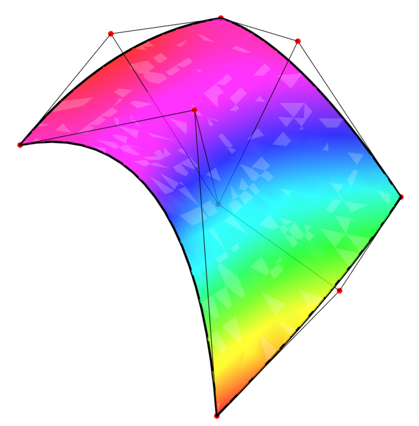
Example 2
We test for coincidence the irreducible surfaces and of degree with control points shown in Table 1. We apply Algorithm 1. The unique solution of system (9) is . Surfaces and are shown in Fig. 2b. and Fig. 2c., respectively. Their coincident part is and it is shown with its control polygon in Fig. 2b.
Example 3
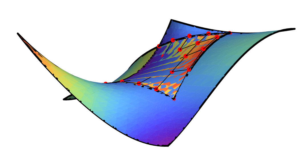
We consider the irreducible surfaces and of degree and , respectively. Their control points are shown in Table 2. This example matches Case 1 of Lemma 4, and hence system (22) has a unique solution =. Surfaces and are shown in Fig. 4a. and Fig. 4b., respectively. They have coincidence and their coincident part is surface , see Fig. 4c.
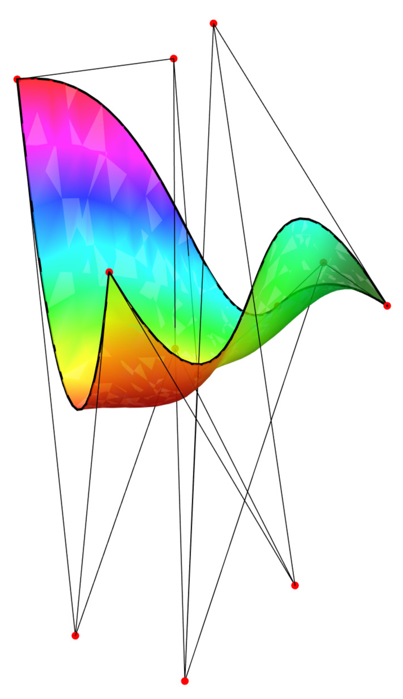
a.

b.
c.
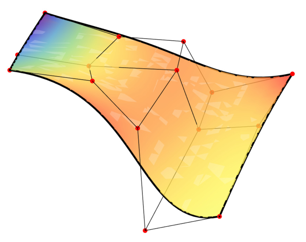
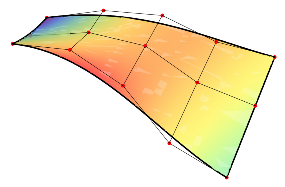
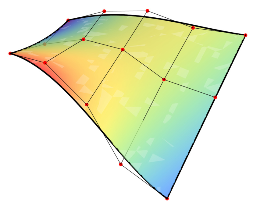
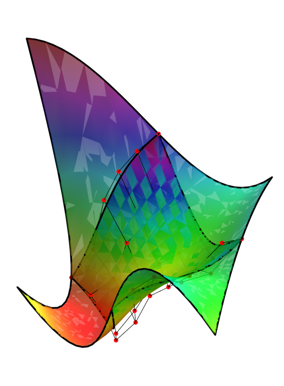
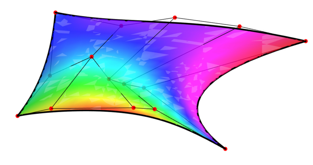
Example 4
We test for coincidence the irreducible surfaces and of degree and , respectively. Their control points are shown in Table 3. The corresponding vectors are coplanar and hence, matrix , defined by (25) has rank 2. We apply Algorithm 2 and obtain the following two solutions to system (23),
The first of these solutions generates TPB surface whose control polygon coincides with the control polygon of . Hence, and have coincidence. Surfaces , , and their coincident part are shown in Fig. 5 The control points of are shown in Table 3.

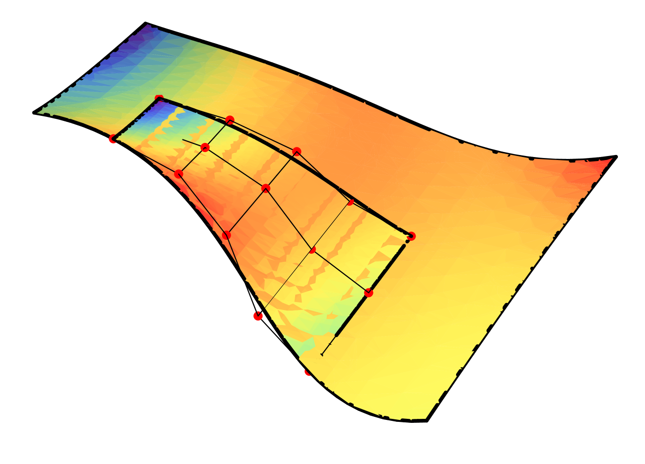
Example 5
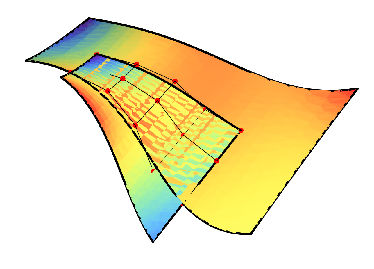
In our final example we test for coincidence the irreducible surfaces and of degree and , respectively. Their control points are shown in Table 4. Surfaces and are shown in Fig. 6a. and Fig. 6b.. The corresponding system (22) has a unique solution =. The shared domain of and is a hexagon. We represent the coincident part as a union of two TPB surfaces and compute their control points using blossoming, see Fig 6c.
a.
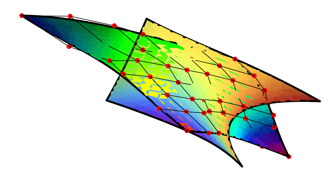
b.
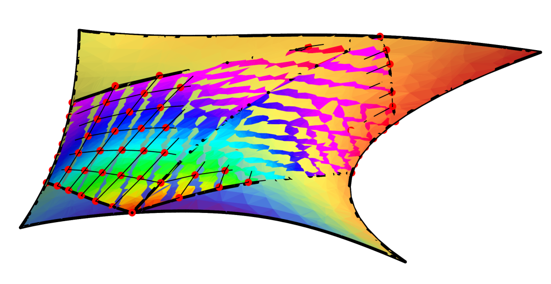
c.
4 Conclusions and future work
In this paper we considered and solved the problem for testing TPB surfaces for coincidence. We presented two different methods and develop two algorithms based on these methods that test two irreducible TPB surfaces for coincidence and report their coincident part if it is present. The first algorithm works for surfaces of same degree and the second one - for surfaces of degree and , respectively. We presented numerical experiments and gave examples to visualize and support the obtained results. Our next task for future research is to develop and implement an algorithm for testing TB surfaces for coincidence.
Acknowledgments
This work was partially supported by Sofia University Science Fund Grant No. 80-10-103/2023.
References
- Barton and Zippel (1985) Barton, D., Zippel, R., 1985. Polynomial decomposition algorithms. J. Symbolic Comput. 1, 159–168. doi:10.1016/S0747-7171(85)80012-2.
- Berry and Patterson (1997) Berry, T., Patterson, R., 1997. The uniqueness of Bézier control points. Comput. Aided Geom. Des. 14, 877–879. doi:10.1016/S0167-8396(97)00016-2.
- Chen and Ma (2015) Chen, X.D., Ma, W., 2015. Rebuttal to “comment on the ‘coincidence condition of two Bézier curves of an arbitrary degree’ ”. Comput. Graph. 53, 167–169. doi:https://doi.org/10.1016/j.cag.2015.10.007.
- Chen et al. (2013) Chen, X.D., W. Ma, W., Deng, C., 2013. Conditions for the coincidence of two quartic Bézier curves. Appl. Math. and Comput. 225, 731–736. doi:10.1016/j.amc.2013.09.053.
- Chen et al. (2016) Chen, X.D., Yang, C., Ma, W., 2016. Coincidence condition of two Bézier curves of an arbitrary degree. Comput. Graph. 54, 121–126. doi:10.1016/j.cag.2015.07.013.
- Denker and Herron (1997) Denker, W., Herron, G., 1997. Generalizing rational degree elevation. Comput. Aided Geom. Des. 14, 399–406. doi:10.1016/S0167-8396(96)00036-2.
- Farin (2002) Farin, G., 2002. Curves and Surfaces for CAGD: A Practical Guide. 5th ed., Morgan-Kaufmann, San Francisco.
- Farouki (2012) Farouki, R., 2012. The Bernstein polynomial basis: a centennial retrospective. Comput. Aided Geom. Des. 29, 379–419. doi:10.1016/j.cagd.2012.03.001.
- von zur Gathen (1990) von zur Gathen, J., 1990. Functional decomposition of polynomials: the tame case. J. Symbolic Comput. 9, 281–299. doi:10.1016/S0747-7171(08)80014-4.
- Goldman (2003) Goldman, R., 2003. Pyramid algorithms: A dynamic programming approach to curves and surfaces for geometric modeling. Elsevier Science (USA).
- Kozen and Landau (1989) Kozen, D., Landau, S., 1989. Polynomial decomposition algorithms. J. Symbolic Comput. 7, 445–456. doi:https://doi.org/10.1016/S0747-7171(89)80027-6.
- Pekerman et al. (2005) Pekerman, D., Seong, J.K., Elber, G., Kim, M.S., 2005. Are two curves the same? Comput.-Aided Des. Appl. 2, 85–94. doi:10.1080/16864360.2005.10738356.
- Snchez-Reyes (2011) Snchez-Reyes, J., 2011. On the conditions for the coincidence of two cubic Bézier curves. J. of Comput. Appl. Math. 236, 1675–1677. doi:10.1016/j.cam.2011.08.024.
- Snchez-Reyes (2014) Snchez-Reyes, J., 2014. The conditions for the coincidence or overlapping of two Bézier curves. Appl. Math. Comput. 248, 625–630. doi:10.1016/j.amc.2014.10.008.
- Snchez-Reyes (2015a) Snchez-Reyes, J., 2015a. Comment on the “coincidence condition of two Bézier curves of an arbitrary degree”. Comput. Graph. 53, 166. doi:10.1016/j.cag.2015.10.006.
- Snchez-Reyes (2015b) Snchez-Reyes, J., 2015b. Detecting symmetries in polynomial Bézier curves. J. of Comput. Appl. Math. 288, 274–283. doi:10.1016/j.cam.2015.04.025.
- Vlachkova (2017) Vlachkova, K., 2017. Comparing Bézier curves and surfaces for coincidence, in: Georgiev, K., Todorov, M., Georgiev, I. (Eds.), Advanced Computing in Industrial Mathematics. Springer International Publishing. volume 681 of LNCS, Studies in Computational Intelligence, pp. 239–250. doi:10.1007/978-3-319-49544-6_20.
- W.-K. Wang et al. (2011) W.-K. Wang, W.K., Zhang, H., Liu, X.M., Paul, J.C., 2011. Conditions for coincidence of two cubic Bézier curves. J. Comput. Appl. Math.. 235, 5198–5202. doi:10.1016/j.cam.2011.05.006.
- Yang and Zeng (2008) Yang, L.Q., Zeng, X.M., 2008. Trimming Bézier surfaces on Bézier surfaces via blossoming, in: Chen, F., Jttler, B. (Eds.), LNCS 4975, Springer, Berlin Heidelberg. pp. 578–584. doi:10.1007/978-3-540-79246-8_50.