Interactive Joint Planning for Autonomous Vehicles

Abstract

In highly interactive driving scenarios, the actions of one agent greatly influences those of its neighbors. Planning safe motions for autonomous vehicles in such interactive environments, therefore, requires reasoning about the impact of the ego’s intended motion plan on nearby agents’ behavior. Deep-learning-based models have recently achieved great success in trajectory prediction and many models in the literature allow for ego-conditioned prediction. However, leveraging ego-conditioned prediction remains challenging in downstream planning due to the complex nature of neural networks, limiting the planner structure to simple ones, e.g., sampling-based planner. Despite their ability to generate fine-grained high-quality motion plans, it is difficult for gradient-based planning algorithms, such as model predictive control (MPC), to leverage ego-conditioned prediction due to their iterative nature and need for gradient. We present Interactive Joint Planning(IJP) that bridges MPC with learned prediction models in a computationally scalable manner to provide us the best of both the worlds. In particular, IJP jointly optimizes over the behavior of the ego and the surrounding agents and leverages deep-learned prediction models as prediction priors that the join trajectory optimization tries to stay close to. Furthermore, by leveraging homotopy classes, our joint optimizer searches over diverse motion plans to avoid getting stuck at local minima. Closed-loop simulation result shows that IJP significantly outperforms the baselines that are either without joint optimization or running sampling-based planning.

I Introduction

A cornerstone for safe motion planning for autonomous vehicles is the ability to reason about interactions between the ego vehicle and other traffic agents, such as human-driven vehicles and pedestrians. A standard approach to deal with interactive scenarios is to leverage prediction models—heuristic [1] or data-driven [2, 3]—to generate predictions of the traffic agents’ future motions and plan the ego motion accordingly. In particular, various deep-learned prediction models now represent the state of the art in prediction [4, 5, 6]. Modern deep learning prediction models widely use ego-conditioning, i.e., condition the prediction of adjacent agents’ motion on the ego’s future motion, to improve the prediction quality and capture the interaction between the ego and the agents. The resulting prediction is then consumed by a planner that aims to generate an ego motion plan that avoids collisions and makes progress towards the goal. Depending on how the prediction is consumed, there are two typical styles of planners: sampling-based planners and iterative planners. The former takes a bunch of ego motion samples, calls the prediction model to generate ego-conditioned predictions and searches for a motion plan [3, 7]. An iterative planner, on the other hand, iteratively refines the ego motion plan, with e.g. gradient [8] or Bayesian optimization [9]. While the latter may achieve finer granularity for the ego motion due to iterative refinement, it needs to evaluate the ego motion plan significantly more times than a sampling-based counterpart and the evaluation cannot be parallelized. As a result, the computational complexity prohibits the use of complex deep-learned ego-conditioned prediction models together with an iterative planner—when a prediction model is used, it is typically limited to simple analytical models [10]. In this paper, we propose a computationally tractable approach, called Interactive Joint Planning (IJP), which reasons about interactivity by combining deep-learned prediction models with iterative planners. IJP significantly outperforms other baselines yielding safer motion plans without sacrificing liveness and being overly conservative.

Contributions and paper organization. We propose IJP, which is a model predictive control (MPC)-based planner that is compatible with any (deep learned) prediction model. The two main novelties are (i) IJP jointly optimizes over the ego vehicle and the nearby agents’ motion with collision avoidance constraints while penalizing deviation from the unconditioned predicted trajectories of the agents. The “planned” motion for the agents then serve as the ego-conditioned trajectory predictions for those agents and are integrated in the gradient-based planner. (ii) To remedy the local minimum issue of nonconvex optimization, we introduce the novel concept of free-end homotopy that allows us to efficiently explore a diverse range of motions. In particular, free-end homotopy is an extension of homotopy to trajectories that do not share the same end point. We empirically show that IJP significantly outperforms a baseline without joint optimization and is superior to a sampling-based planner baseline in both performance and computation complexity.

II Related Works

Interactive Planning. Interactive / social-aware planning has been studied extensively in the literature. Some of the early approaches modeled the uncontrolled agents’ behavior as Gaussian uncertainty [11] without consideration for the impact of ego behavior on nearby agents. Ignoring the ego’s impact can lead to overly conservative motion plans as was famously shown in the freezing robot problem [12]. This led to a plethora of research on navigating crowds while accounting for the reactivity of other agents, such as the joint optimization via Gaussian Process (GP) approach in [12, 13] and the reinforcement learning (RL) approach in [14].

Reactive Behavior Modeling. The crux of interactive planning is to properly model other agents’ reactive behavior. Inverse reinforcement learning (IRL) [15] is an obvious choice, e.g., in [16, 17], and it is used subsequently in optimization over the ego motion [18, 19]. Another popular formulation leverages game theory, which assumes that every agent tries to maximize its own utility [20, 21]; however, the computational complexity of equilibrium solving remains a challenge and it is not straightforward to combine game theory with data-driven methods. Partially-observable Markov Decision Process (POMDP)-based methods were applied to interactive planning and inferring the hidden intention of surrounding agents [22, 23], but similar to the game-theoretic approaches, POMDPs also suffer from high computational complexity and they are typically hand-crafted, making them difficult to scale. Other analytical models such as Intelligent Driver Models (IDM) [24] and Probabilistic Graphic Models (PGM) [25] have also been applied to intention estimation and interactive planning, however, they are limited to simple scenarios, such as highway driving. The idea of joint optimization has been studied for conflict resolution [26], yet assumes knowledge about the other agent’s cooperativeness.

Deep-Learned Prediction. The above-mentioned methods, though very different in nature, all make assumptions (e.g. rationality) about the surrounding agents’ decision processes, and the planner then leverages the assumptions to make the planning problem tractable. In contrast, modern prediction methods are predominantly deep-learned phenomenological models [6, 27, 28, 4, 5], i.e., models trained with data to match the ground truth without a clear explanation of the decision process. While they achieve good prediction accuracy and are capable of ego-conditioned prediction, working with downstream interactive planner remains difficult, as pointed out previously. The expensive inference of ego-conditioned prediction under a large number of ego plans made it prohibitive to evaluate fine-grained ego plans. In [29] the authors use a linear system to represent the ego-conditioned prediction compactly, but the performance is limited by the simplicity of linear systems.

Homotopy Planning. Homotopy planning has been widely studied for motion planning of autonomous systems. To distinguish among homotopy classes of trajectories, [30] uses the relative lateral position (i.e., left or right) between two vehicles, [31, 32] partition the free space into sub-regions, [33, 34] construct homotopy-invariant words, while [35, 36] use a magnetic-field inspired approach. All these approaches require the start and end points of all candidate trajectories to coincide for homotopy classes to be well-defined—there exists no concept in the literature on homotopy that accommodates distinguishing trajectories that do not share the same end point. In this paper, we generalize homotopy to rigorously develop the notion of free-end homotopy which provides the same benefits as homotopy to motion planning, but for trajectories that do not share the same end point.

III Free-end Homotopy Classes

In this section, we will introduce the notion of free-end homotopies that will facilitate faster planning by reducing the number of trajectory initializations for the joint optimization.

III-A Background: Introduction to Homotopy

Homotopy classes are defined as follows:

Definition 1 (Homotopy Class [35])

Two continuous trajectories $\mathbf{x}_{1}:\mathbb{R}\to\mathcal{X}$ and $\mathbf{x}_{2}:\mathbb{R}\to\mathcal{X}$ connecting the same start and end coordinates $x_{s}$ and $x_{g}$, respectively, belong to the same homotopy class if and only if one can be continuously deformed into the other without intersecting any obstacles.

Remark 1

It should be clarified that homotopy is not enforced in an open-ended trajectory optimization problem and it is the limitation of gradient-based optimization that causes the local miminum issue. Nonetheless, studying homotopy offers an intuitive way to partition the solution space into disjoint subsets.

Directly checking Definition 1 to verify if two trajectories belong to the same homotopy class is not straightforward. Multiple approximation methods and work-arounds have been proposed in the literature. [30] use the relative lateral position (left or right) when two vehicles longitudinal location coincides to determine the homotopy class, yet the criteria is ambiguous as the direction of longitudinal and lateral is not clear in scenarios with curving roads and intersections. In [31] the authors partition the free space into non-intersecting polytopes and use the order of region traversing to identify homotopy classes. However, free space partitioning is expensive and only works for static environments. A more common implicit approach is to use multiple trajectory samples as initialization for the gradient-based planner and hoping that one of the solutions is the global optimum [37]. However, it is generally inefficient with random initialization as many optimization instances will converge to the same local minimum.

A key feature of planning for AVs is that the motion plan may not have a fixed end point. For instance, if we require the AV to progress along the road while avoiding obstacles, a particular goal state is not prescribed to the planner. To account for this, we will introduce the notion of free-end homotopy by using magnetic-field homotopy introduced in [35].

III-B Introduction to Magnetic-Field-Based Homotopy

The magnetic field approach for homotopy class verification [35] is based on Ampere’s law:

$$\oint_{C}\mathbf{B}\cdot d\mathbf{l}=\mu_{0}I_{\text{enc}},$$

which states that the line integral of magnetic field around a closed curve is equal to the product of the magnetic constant $\mu_{0}$ and the current enclosed $I_{\text{enc}}$. Ampere’s law establishes an equivalence condition among all closed curves that encloses the same current, which can also be extended to curves sharing the same starting and ending position. Applying this to homotopy classes in motion planning, the authors in [35] let obstacles carry current and calculate the Ampere circuit integral along the robot’s trajectory, which is then used to categorize trajectories into different homotopy classes.

In 2D space, all obstacles can be viewed as having genus (number of holes) 0 and the imaginary current can be set perpendicular to the X-Y plane crossing the center of the obstacle. Furthermore, the path integral of the magnetic field is easy to compute in 2D; specifically, using Biot-Savart law, the magnetic field near an infinitely long wire at point $p$ with current $I$ perpendicular to the X-Y plane is given by

$$\mathbf{B}(\mathbf{r})=\frac{\mu_{0}I}{2\pi||\mathbf{r}||},$$

and the direction follows the right-hand law. It follows that the path integral of the magnetic filed along a directional curve that does not intersect with $p$ is simply $\frac{\mu_{0}I}{2\pi}\Delta\theta$, where $\Delta\theta$ is the angular distance from the start to the end. Fig. 1 illustrates an example where the obstacle is marked in green and the imaginary current that goes through its center $p$, generating a magnetic field $\mathbf{B}$, visualized with the dashed lines. The path integral is then proportional to the angular distance from the start to the end point of the curve. Note that the angular distance is directional and can be negative; when the curve circles $p$ counter-clockwise /clockwise once, the angular distance increases/decreases by $2\pi$, respectively. The angular distance provides two major benefits: (i) it is easy to compute and enforce as a constraint, and (ii) it can be easily extended to moving obstacles, as discussed next.

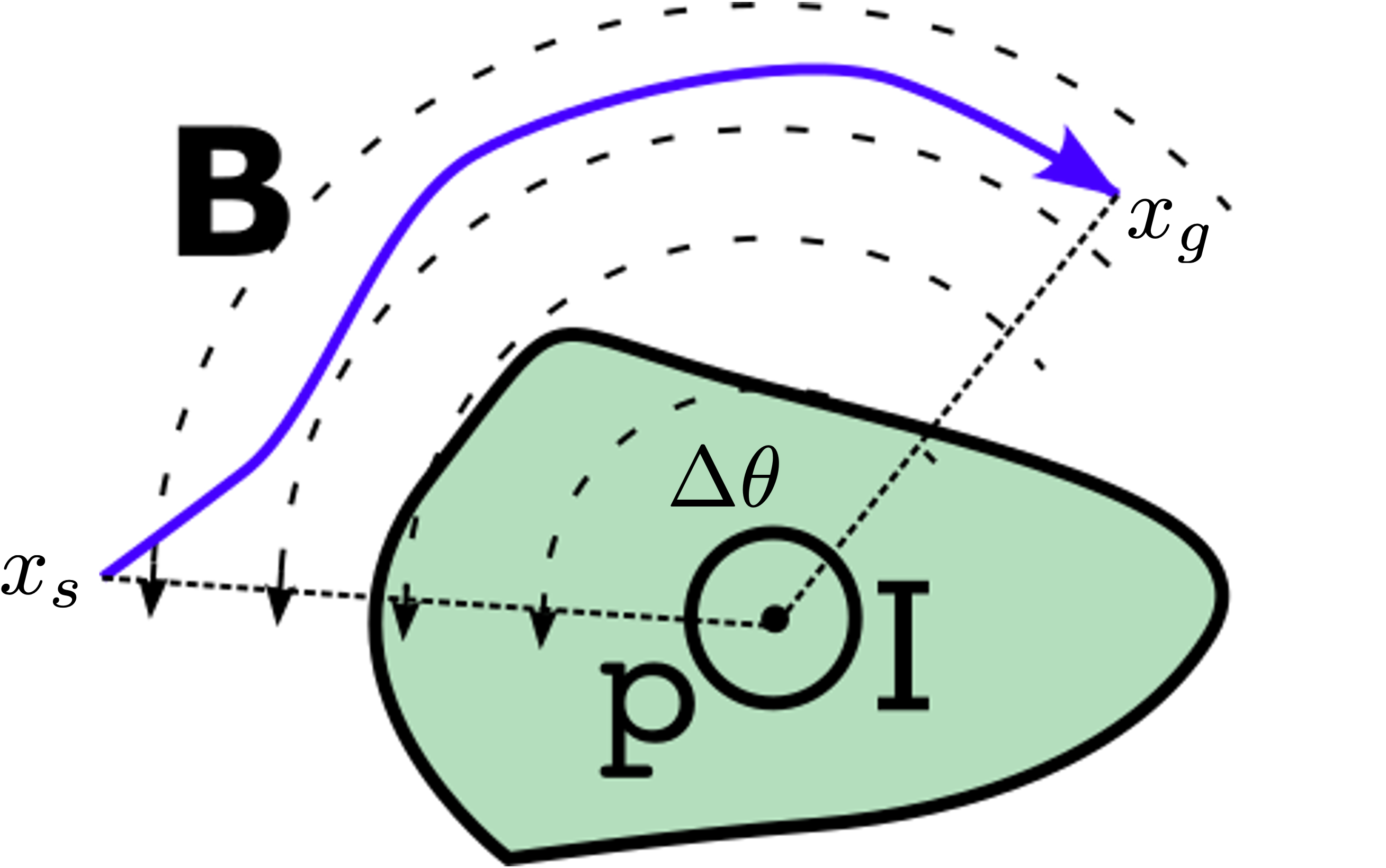
Figure 1: Magnetic path integral in 2D

Let $\mathbf{x}$ be the trajectory of the ego and $\mathbf{x}^{\rm o}$ be the trajectory of an obstacle. To calculate the angular distance $\Delta\theta$, discretize the (X,Y) coordinates of the curves $\mathbf{x}$ and $\mathbf{x}^{\rm o}$ into a sequence of waypoints $\{(X_{i},Y_{i})\}_{i=1}^{N}$, $\{(X^{\rm o}_{i},Y^{\rm o}_{i})\}_{i=1}^{N}$ and $\Delta\theta$ is computed as

$$\Delta\theta(\mathbf{x},\mathbf{x}^{\rm o}):=\sum_{i=1}^{N-1}\arctan\frac{Y_{i+1}-Y^{\rm o}_{i+1}}{X_{i+1}-X^{\rm o}_{i+1}}-\arctan\frac{Y_{i}-Y^{\rm o}_{i}}{X_{i}-X^{\rm o}_{i}}$$ (1)

It is clear that (1) applies to moving obstacles as well.

III-C Free-end Homotopy

As mentioned above, the motion planning problem for AV may not have a fixed end point. Homotopy classes are not well-defined for two curves with different ending points. To resolve this issue, we introduce free-end homotopy, an extension of homotopy, for trajectories that share the same initial point but different end point. The overarching objective is to develop an equivalence class of trajectories, which we call free-end homotopy classes, whose members execute the same relative motion with respect to other agents (e.g., overtake from left of agent 1 and stay behind agent 2) while being continuously transformable to any other member in the class. Free-end homotopy classes facilitate efficient planning by allowing us to downsample motion plan candidates to only those that belong to different free-end homotopy classes, i.e., ones with different relative motions with respect to obstacles.

Let $\mathbf{x}$ be the trajectory of the ego and $\mathbf{x}^{\rm o}$ be the trajectory of a particular obstacle. We begin by defining the mode $m:(\mathbf{x},\mathbf{x}^{\rm o})\mapsto m(\mathbf{x},\mathbf{x}^{\rm o})\in\mathbb{Z}$ of a trajectory with respect to a particular obstacle using the angular distances $\Delta\theta$:

$$m(\mathbf{x},\mathbf{x}^{\rm o}):=\left\{\begin{aligned} -(k+1),&&-(\hat{\theta}+k\pi)\leq\Delta\theta(\mathbf{x},\mathbf{x}^{\rm o})<-(\hat{\theta}+(k+1)\pi)\\ 0,&&-\hat{\theta}\leq\Delta\theta(\mathbf{x},\mathbf{x}^{\rm o})<\hat{\theta}\\ k+1,&&\hat{\theta}+k\pi\leq\Delta\theta(\mathbf{x},\mathbf{x}^{\rm o})<\hat{\theta}+(k+1)\pi\end{aligned}\right.$$ (2)

where $\hat{\theta}$ is a suitably large threshold for differentiating between the three modes. We refer to these three classes as clockwise (CW), stationary (S), and counter-clockwise (CCW), as illustrated in Fig. 2. In CW mode, the ego vehicle moves clockwise relative to the object, in CCW the ego vehicle moves counter-clockwise relative to the object, while in S, the ego vehicle remains roughly static relative to the object.

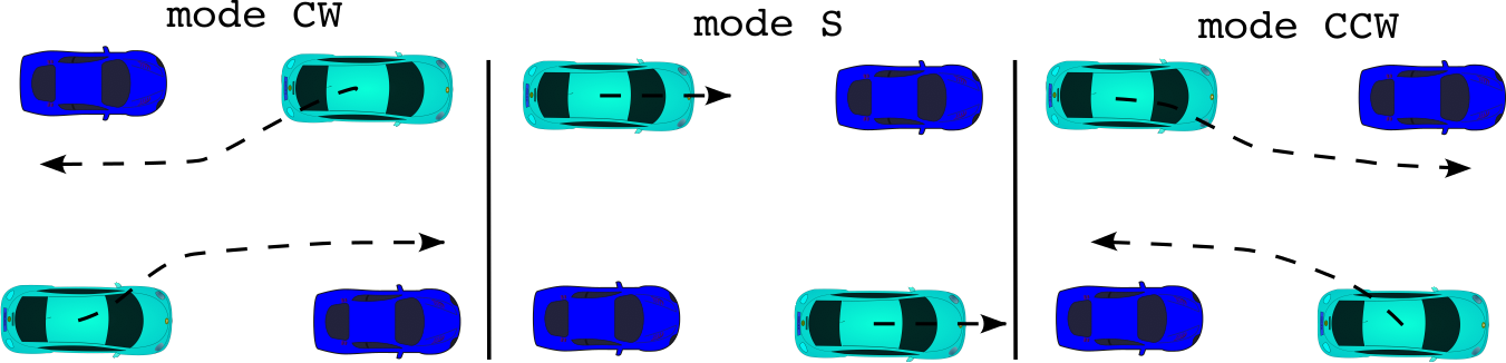
Figure 2: Three homotopy classes: CW, S, and CCW

Remark 2

Modes with more refined quantization, e.g. consider $\Delta\theta\in[k\pi,(k+1)\pi]$, can be chosen. We chose only three categories as they were found to be sufficient to cover the typical driving scenarios.

If there are $M$ obstacles in the scene, then the mode vector $h$ for an ego trajectory $\mathbf{x}$ is defined as the cartesian product of the modes (2) with respect to each obstacle in the scene, i.e., $h(\mathbf{x},\{\mathbf{x}_{i}^{\rm o}\}_{i=1}^{M}):=(m(\mathbf{x},\mathbf{x}_{1}^{\rm o}),\cdots,m(\mathbf{x},\mathbf{x}_{M}^{\rm o}))$; Fig. 3 illustrates $h$ with an example scene with two cars near the ego vehicle and three example trajectories. With this, we are now ready to define free-end homotopy.

Definition 2 (Free-end Homotopy)

Let $\mathbf{x}_{1}:\mathbb{R}\to\mathcal{X}$ and $\mathbf{x}_{2}:\mathbb{R}\to\mathcal{X}$ be two continuous trajectories that share the same start point, but do not necessarily share the same end point. Then, a continuous mapping $f:[0,1]\times\mathbb{R}\to\mathcal{X}$ is called a free-end homotopy if it satisfies the following criteria:

• $f(0,\cdot)=\mathbf{x}_{1}(\cdot)$,

• $f(1,\cdot)=\mathbf{x}_{2}(\cdot)$, and

• for all $\lambda\in[0,1]$, the mode vector $h_{\lambda}$ for $f(\lambda,\cdot)$ are equal.

If a free-end homotopy $f$ exists between $\mathbf{x}_{1}$ and $\mathbf{x}_{2}$, then the two trajectories are said to be free-end homotopic.

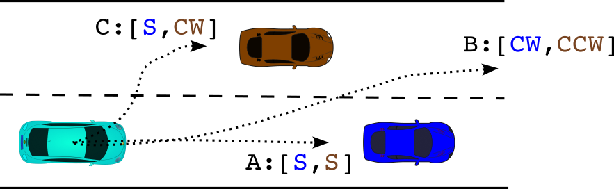
Figure 3: Homotopy classes for two nearby objects where trajectory A is categorized as S for both objects; trajectory B is categorized as CW for the blue car and CCW for the brown car; and trajectory C is categorized as S for the blue car and CW for the brown car.

Free-end homotopy is a generalization of the notion of homotopy. We make this clear in the next lemma which shows that all homotopic trajectories (with the same start and end points), are also free-end homotopic.

Lemma 1

Continuous trajectories with same start and end points are homotopic, if, and only if, they are also free-end homotopic. Furthermore, the homotopy is also a free-end homotopy.

Proof:

Proof provided in the appendix. ∎

In the next lemma we show that the free-end homotopy relation defined above is, in fact, an equivalence relation.

Lemma 2 (Free-end homotopy is an equivalence relation)

Free-end homotopy, presented in Definition 1, is an equivalence relation.

Proof:

Proof provided in the appendix. ∎

This result ensures that all trajectories that are free-end homotopic can be continuously transformed from one to another while retaining the same mode vector. Hence, we can limit our planning to just one candidate per free-end homotopy class. However, it remains unresolved whether all trajectories with the same mode vector belong to the same free-end homotopy class. Indeed, in the next theorem we will show that only one free-end homotopy class corresponds to one mode vector. This ensures that if we find a continuous trajectory with a particular mode vector, we can continuously transform it to any other trajectory with the same mode vector, since they all belong to the same free-homotopy class. This facilitates faster planning by letting us run a continuous optimizer (as discussed later in Section IV) on only one trajectory per mode vector.

Theorem 1 (One free-end homotopy class per mode vector)

Continuous trajectories with the same mode vector are free-end homotopic.

Proof:

The proof is provided in the appendix. ∎

III-D Applying free-end homotopy classes in motion planning

When initializing a motion planner, a naive choice is to consider all possible free-end homotopy classes, however, the number of free-end homotopy classes grows exponentially with the number of nearby objects and many of the classes are not realistic. For example, in the situation depicted in Fig. 3, CCW for the blue vehicle is not viable as there is not enough space to pass by its right side. For faraway objects, the free-end homotopy class is most likely S due to a small angular distance within the planning horizon.

To identify the promising free-end homotopy classes, we take a sampling approach. Specifically, we use a trajectory sampler to generate $N$ trajectory samples for the ego vehicle. Then we invoke a trajectory predictor to provide scene-centric trajectory predictions for all $M$ objects in the scene. Together there are $N\times M$ free-end homotopy class candidates that are expressed as mode vectors, as described in Section III-C. Among these $N\times M$ mode vectors, many result in repeated mode vectors. Leveraging Theorem 1, we only retain the trajectory with the highest reward among all trajectories sharing the same mode vector as a representative for the corresponding free-end homotopy class. The reward function can be any scalar-valued function that scores the performance of the ego trajectory sample amidst the objects’ prediction.

Now that we are left with $K$ trajectories out of the $N\times M$ candidates, each with a unique free-end homotopy class for the whole scene, an ego trajectory sample and predictions for the objects. These $K$ trajectories are used to initialize the gradient-based motion planner in two ways: (i) the nonlinear planning problem is linearized around the ego and the objects’ trajectories to create an efficiently-solvable sequential quadratic program (SQP), and (ii) the free-end homotopy class of the trajectory is enforced as a constraint in the planning problem.

IV Method

As discussed in the introduction, modern trajectory planners for autonomous vehicles rely on predictions for nearby agents, and ego-conditioning has been shown to improve the planning performance yet is expensive to run. The proposed IJP does not require ego-conditioned predictions, but replaces them with a joint optimization. Specifically, we invoke a prediction module to forecast the non-ego-conditioned future trajectories of the surrounding agents and pass them to the MPC planner. Intuitively, this prior supplies the optimizer with the non-ego agents’ intent. The MPC planner then plans for both the ego vehicle and the surrounding agents to minimize the cost function, which we shall discuss in detail later, while enforcing collision avoidance constraint. In reality, the AV can only control its owm motion, thus assuming control over surrounding agents without any limitation is obviously naive. To remedy this, the cost contains two terms, a term that penalizes nearby agents’ deviation from the predicted trajectories, and a term that penalizes their acceleration and jerk. These two terms are interpreted as the price for the ego to force nearby agents away from their nominal path.

The resulting “planned” trajectories of nearby agents can be viewed as the ego-conditioned prediction that roughly centers around the unconditioned trajectory prediction. Fig. 9 illustrates the joint optimization as ego-conditioned prediction. The dashed line shows the unconditioned prediction for the blue agent, which comes from the trajectory predictor; the joint optimization then choose to let the ego (red) change lane and let the blue agent swerve to avoid a collision with the ego, which is viewed as the ego-conditioned prediction, and the deviation from the unconditioned prediction is penalized.

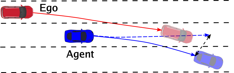
Figure 4: Joint optimization as ego-conditioned prediction: solid trajectories: solution of the joint optimization; dashed line unconditioned predicted trajectory of the blue agent.

Since the prediction model is only called once without ego-conditioning, the inference time decreases significantly. Moreover, the joint optimization result provides a much finer granularity compared to running ego-conditioned prediction on ego trajectory samples.

Next, we break down the key components of the joint MPC.

IV-A Dynamic constraints

We use a Dubin’s car model for all vehicles and cyclists in the scene (including the ego vehicle).

$$x=\begin{bmatrix}X\\ Y\\ v\\ \psi\end{bmatrix},u=\begin{bmatrix}\dot{v}\\ \dot{\psi}\end{bmatrix},x^{+}=\begin{bmatrix}X+v\cos(\psi)\Delta t\\ Y+v\sin(\psi)\Delta t\\ v+\dot{v}\Delta t\\ \psi+\dot{\psi}\Delta t\end{bmatrix}.$$ (3)

where $X,Y$ are the longitudinal and lateral coordinates, $v$ and $\dot{v}$ are the longitudinal velocity and acceleration, $\psi$ and $\dot{\psi}$ are the heading angle and yaw rate.

The pedestrians follow a double integrator model with the following dynamics:

$$x=\begin{bmatrix}X\\ Y\\ v_{x}\\ v_{y}\end{bmatrix},u=\begin{bmatrix}\dot{v}_{x}\\ \dot{v}_{y}\end{bmatrix},x^{+}=\begin{bmatrix}X+v_{x}\Delta t\\ Y+v_{y}\Delta t\\ v_{x}+\dot{v}_{x}\Delta t\\ v_{y}+\dot{v}_{y}\Delta t\end{bmatrix}.$$

These dynamic models are linearized around an initial guess of $x,u$ pair generated by a trajectory sampler as mentioned in Section III. The initial guess satisfies the nonlinear dynamic equations, and the linearized dynamic model takes the form $x^{+}=Ax+Bu+C$.

Furthermore, we impose dynamic constraints on state and inputs of the agents. Specifically, for all vehicles,

$$v\in[v^{\min},v^{\max}]$$ (4)

$$|v\dot{\psi}|\leq a_{y}^{\max}$$ (5)

$$|\psi|\leq\frac{\delta^{\max}}{l}|v|$$ (6)

$$\dot{v}\in[a_{x}^{\min},a_{x}^{\max}],$$ (7)

where $[v^{\min},v^{\max}]$ is the velocity range, $a_{y}^{\max}$ is the maximum lateral acceleration, $a_{x}^{\min}$ and $a_{x}^{\max}$ are the lower and upper bounds for longitudinal acceleration, $\delta^{\max}$ is the maximum steering angle and $l$ is the distance between the front and rear axles. All pedestrians follow a simple norm bound on velocity and acceleration:

$$||v||\leq v_{\max},\quad||\dot{v}||\leq\dot{v}_{\max}.$$

The dynamic constraints are linearized (especially (6) so that the effect of velocity is accounted for) and the linearized constraints is written as $G_{x}^{d}x+G_{u}^{d}u\leq g^{d}$.

IV-B Safety constraints

Safety constraints mainly consist of two parts, collision avoidance constraints and lane boundary constraints.

All vehicles are modeled as rectangles with varying size (including the ego) and the pedestrians are modeled as a circle with varying radius. The collision avoidance between the ego (rectangle) and pedestrians (circles) is encoded by checking the three cases where the maximum margin is achieved on the X axis, Y axis, and corners of the vehicle, as shown in Fig. 5. For two vehicles, we analytically calculate the 4 polytopic free spaces around one of the vehicles, as shown in Fig. 5, and enforce linear constraints that the other vehicle’s 4 corners and center point all lie in one of the free spaces. Then we do the same after reversing the role of the two vehicles.

Figure 5: Collision checks between vehicles and pedestrians (left), and two vehicles (right)

In addition to the collision avoidance constraints, we also enforce the homotopy class constraint, which is computed as discussed in Section III. In simulation we observed that the MPC QP behave similarly without the homotopy constraint and the initialization/linearization is sufficient to enforce the homotopy constraint.

Lane boundaries are given as polylines (sequence of waypoints with headings), the lane boundary constraints are enforced by projecting the vehicle centers to the polylines and calculate the distance margins, as shown in Fig. 6.

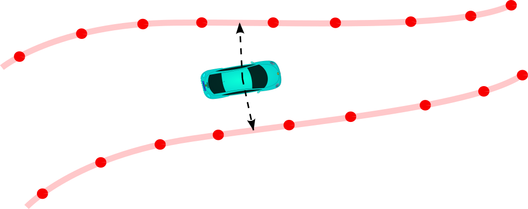
Figure 6: Lane boundary constraint

All of the above mentioned inequality constraints are differentiable w.r.t. the state of the ego vehicle and other agents on the road, and they are linearized and enforced as linear constraints in the MPC. To ensure feasibility, we add slack variable to collision avoidance constraints and lane boundary constraints.

IV-C Costs and MPC QP setup

The cost function consists of 5 terms:

• Penalty on ego vehicle’s tracking error w.r.t. the reference trajectory

• Penalty on ego vehicle’s acceleration and jerk

• Penalty on nearby agents’ deviation from their unconditioned trajectory prediction

• Penalty on nearby agents’ acceleration and jerk

Putting all components together, the joint MPC solves the following QP:

$$\mathop{\min}\limits_{\operatorname{\mathbf{u}_{e}},\operatorname{\mathbf{u}_{o}},\operatorname{\mathbf{x}_{e}},\operatorname{\mathbf{x}_{o}}} \eta_{e}(\operatorname{\mathcal{J}_{\text{ref}}}(\operatorname{\mathbf{x}_{e}},\operatorname{\mathbf{x}_{\text{ref}}})+\operatorname{\mathcal{J}_{\text{u}}}(\operatorname{\mathbf{u}_{e}}))+\eta_{o}(\operatorname{\mathcal{J}_{\text{dev}}}(\operatorname{\mathbf{x}_{o}},\operatorname{\mathbf{x}_{\text{pred}}})+\operatorname{\mathcal{J}_{\text{u}}}(\operatorname{\mathbf{u}_{o}}))$$ (8)

$$\mathrm{s.t.}\; x_{e}[0]=x_{e}^{0},\;x_{o}[0]=x_{o}^{0}$$ (9)

$$\forall t=0,...,T-1,i\in\{e,o_{1},...o_{n}\},$$

$$\quad x_{i}[t+1]=A_{i}[t]x_{i}[t]+B_{i}[t]u_{i}[t]+C_{i}[t]$$ (10)

$$\quad G_{x,i}^{d}[t]x_{i}[t]+G_{u,i}^{d}[t]u_{i}[t]\leq g^{d}[t]$$ (11)

$$\forall t=1,...,T,G_{e}^{s}[t]x_{e}[t]+G_{o}^{s}[t]x_{o}[t]\leq g^{s}[t],$$ (12)

where $x_{e}$ is the future state of the ego vehicle, $x_{o_{i}}$ is the future state of agent $i$, $A,B,C$ are the matrices corresponding to the dynamic equality constraints, $G_{x}^{d},G_{u}^{d},g^{d}$ are matrices corresponding to the input and state bounds, $G_{e}^{s},G_{o}^{s},g^{s}$ define the safety constraints, including collision avoidance, lane boundary, and the homotopy constraint.

The costs include $\operatorname{\mathcal{J}_{\text{ref}}}$ that prompts the ego vehicle to track the desired trajectory, $\operatorname{\mathcal{J}_{\text{u}}}$ that penalizes acceleration and jerk (both angular and linear), and $\operatorname{\mathcal{J}_{\text{dev}}}$ that penalizes agents’ deviation from their predictions. $\eta_{e}$ and $\eta_{o}$ determine the distribution of emphasis on the ego vehicle and the agents. A large $\eta_{e}$ leads to more selfish and intrusive behavior of the ego and a small $\eta_{e}$ leads to more altruistic ego behavior.

IV-D Interactive Joint Planning

The IJP planner is summarized in Algorithm 1. The inputs are the reference trajectory for the ego vehicle given by some high-level planner, scene context $\mathbf{C}$, lane information $\mathbf{L}$, and the current state of the ego and surrounding agents.

Firstly, IJP calls the trajectory prediction model to generate predictions for the $M$ surrounding agents from the scene context $\mathbf{C}$. IJP can work with any prediction model that generates dynamically feasible trajectories for the agents involved. It is preferred that the prediction is scene-centric, i.e., predicting joint trajectories for all agents involved. We use Agentformer [6] as our default predictor because it is scene-centric, and is shown to work well with the downstream planner in [7].

Figure 7: Overview of IJP: the trajectory predictor takes in the lane graph and the agent history to predict the unconditioned prediction for the agents $\operatorname{\mathbf{x}_{\text{pred}}}$; the route planner plans the desired route and generates the reference trajectory $\operatorname{\mathbf{x}_{\text{ref}}}$ and distills the lane information (such as lane boundaries) $\mathbf{L}$; the trajectory sampler samples the ego trajectory samples, and together with $\operatorname{\mathbf{x}_{\text{pred}}}$, the homotopy candidates are identified. Finally, IJP plans the ego motion via solving the joint model predictive control problem with SQP.

Algorithm 1 IJP

1:procedure IJP($\operatorname{\mathbf{x}_{\text{ref}}},\mathbf{C},\mathbf{L},x_{e}^{0},x_{o}^{0}$)

2:     $\{\mathbf{x}_{o,j}^{\text{pred}}\}_{j=1}^{M}\leftarrow\textsc{Traj\_pred}(\mathbf{C})$

3:     $\{\mathbf{x}^{\text{sample}}_{e,i}\}_{i=1}^{N}\leftarrow\textsc{Ego\_sampling}(x_{e}^{0},\mathbf{L})$

4:     $\{(\mathbf{x}_{e,k},\mathbf{x}_{o,k},h_{k})\}_{k=1}^{K}\leftarrow\textsc{Hom\_sel}(\{\mathbf{x}^{\text{sample}}_{e,i}\}_{i=1}^{N},\mathbf{x}_{o}^{\text{pred}})$

5:     for $r=1,...,R$ do

6:         for $k=1,...,K$ do

7:              $\text{QP}_{k}\leftarrow\textsc{Linearize}(\operatorname{\mathbf{x}_{\text{ref}}},\mathbf{x}_{e,k},\mathbf{x}_{o,k},h_{k},x_{e}^{0},x_{o}^{0},\mathbf{L})$

8:              $\mathbf{x}_{e,k},\mathbf{x}_{o,k}\leftarrow\textsc{Solve\_QP}(\text{QP}_{k})$

9:         end for

10:     end for

11:     return $\operatorname{\mathbf{x}_{e}}$ associated with the best homotopy class.

12:end procedure

Ego_sampling takes the ego state and lane information to generate ego trajectory samples with a spline sampler introduced in [7], which is then used to identify promising homotopies with the predicted trajectories of the surrounding agents in Hom_sel. With the homotopies selected, IJP uses automatic differentiation to linearize the costs, constraints, and dynamics to formulate a quadratic program. JAX [38] is used for auto-differentiation, and thanks to its powerful parallelization functionality and Just-In-Time (JIT) compilation, the linearization can be done simultaneously for all homotopy classes. The generated QP is solved with 3rd party QP solvers such as GUROBI [39] and Forces Pro [40]. In a sequential quadratic programming (SQP) manner, the nonlinear trajectory optimization problem is linearized and solved as a QP for multiple rounds, each round takes the solution from the last round as the updated linearization point. A proximal constraint is also added to limit the difference of solutions in between rounds to stabilize the SQP.

Remark 3

When the trajectory prediction module outputs multimodal predictions of the surrounding agents, the criteria for selecting the optimal solution among the candidate homotopy classes should also take into account the likelihood of the prediction modes, however, we observed that the mode probabilities predicted by the prediction module is usually of bad quality and thus we ignore the mode probability in the final solution selection and simply choose the mode with the lowest cost. We shall investigate how to incorporate prediction likelihood in solution selection in future work.

V Simulation setup and results

V-A Simulation evaluation setup

We conduct closed-loop simulation in nuPlan [41] to evaluate the proposed approach. The closed-loop planner consists of three modules, a trajectory predictor that generates the unconditioned trajectory prediction, a route planner that distills lane information and reference trajectory from the lane graph, and IJP that plans the trajectory, as shown in Fig. 8.

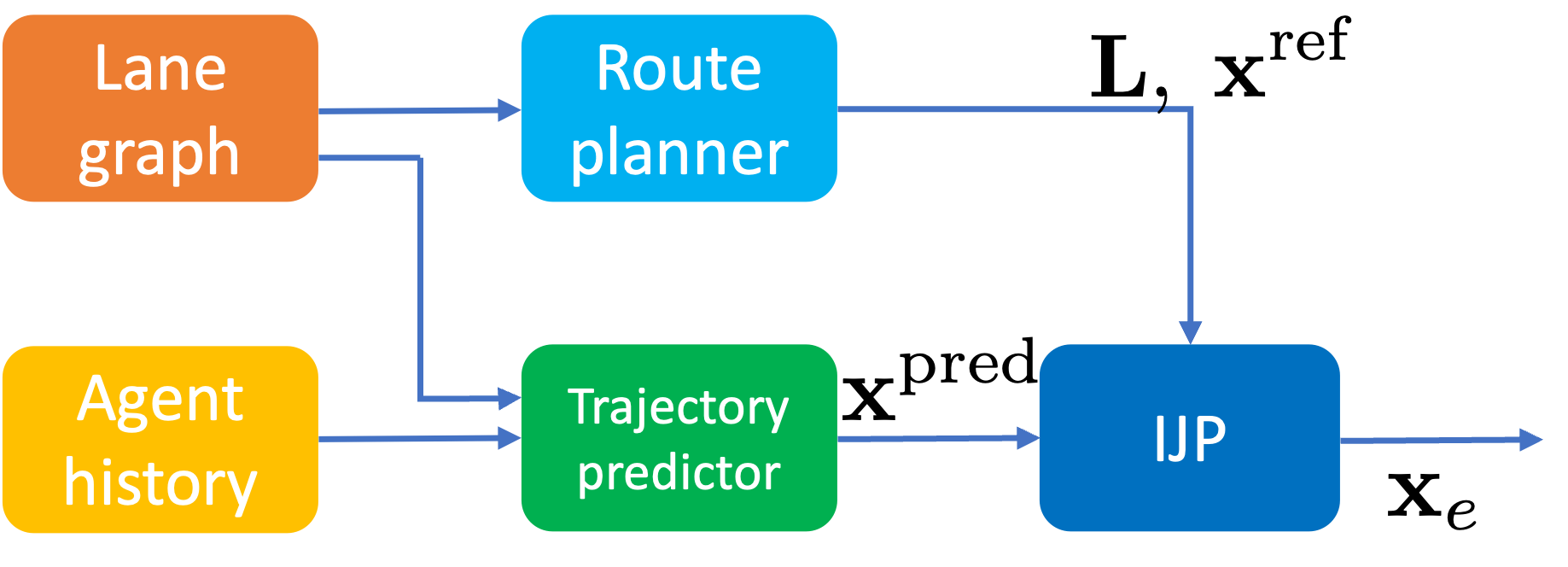
Figure 8: Closed-loop planner structure: the trajectory predictor takes in the lane graph and the agent history to predict the unconditioned prediction for the agents $\mathbf{x}_{\text{pred}}$; the route planner plans the desired route and generates the reference trajectory $\operatorname{\mathbf{x}_{\text{ref}}}$ and distills the lane information (such as lane boundaries) $\mathbf{L}$, and finally IJP plans the ego motion.

We use AgentFormer [6] as the trajectory predictor without ego-conditioning, which generates 4 samples of predicted future trajectories lasting for 3 seconds.

Route planner. The route planner takes the lane graph and the ego state as input, and performs a depth-first search to identify the optimal lane sequence. In nuplan simulation, no goal location is provided, instead the lane segments are labeled as ”on-route” or ”not on-route”. The route planner’s search criteria is to find the an on-route lane sequence (up to a certain depth) that balances (i) distance to the ego vehicle (ii) length of the lane plan and (iii) total curvature of the lane plan. With a lane sequence selected, the reference trajectory is generated by projecting the ego’s current position to the lane centerline and interpolating given the desired ego velocity.

To keep the QP complexity tractable, IJP only include a subset of nearby agents in the joint optimization, denoted as EC agents; the rest of the agents are denoted as non-EC agents and IJP simply encode collision avoidance constraint with their predicted trajectories. The assignment of EC and non-EC agents is based on their minimum distance to the ego vehicle along their predicted trajectories. When there are less agents than the prescribed number, the MPC QP is padded with dummy agents.

To avoid frequent JIT compilation, the number of EC agents and non-EC agents are fixed so that the MPC QP maintains a fixed problem dimension. When the number of nearby obstacles is larger than the sum of the prescribed number of EC and non-EC agents, far away obstacles are simply ignored.

We compare the performance of IJP to two baselines: (i) non-EC MPC: IJP without joint optimization, which only plan the ego behavior and try to avoid collision with the predicted trajectories of nearby agents. (ii) TPP: a sampling-based planner using ego-conditioned prediction, similar to TPP [7] but without multi-layer policy planning.

Remark 4

For fairness of comparison, the non-EC MPC considers a fixed number of non-EC agents, and the number is equal to the sum of EC agents and non-EC agents considered by IJP. The TPP planner instead considers all agents detected as the sampling-based algorithm does not require a fixed number of agents.

V-B Simulation result

Fig. 9 shows an example snapshot from the nuPlan simulation of IJP where the two plots are the MPC solutions under two homotopy classes. The only difference between the two homotopy classes is the homotopy w.r.t. the circled vehicle: S (static) in the left case and CW (clockwise) in the right case. The blue curve is the solution of the EC agents’ trajectories ”planned” by IJP. In the right plot, as the ego (red) change lane, the trailing vehicle changes lane to the right to avoid collision with the ego vehicle, which is indeed similar to an ego-conditioned prediction.

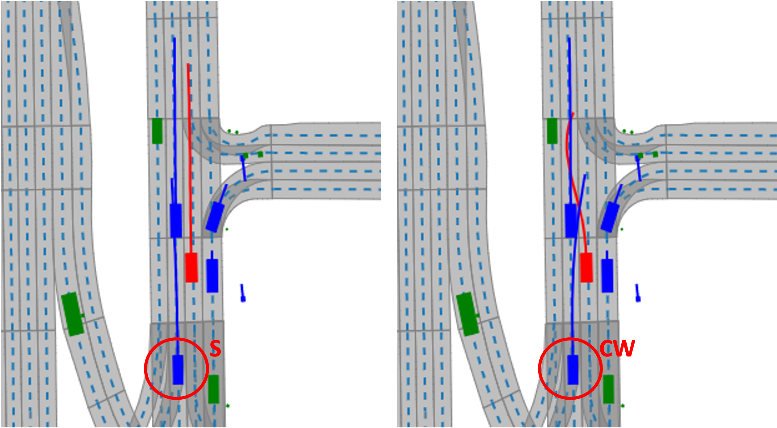
Figure 9: Comparison of the solutions under two homotopy classes: the ego vehicle is in red, the EC agents are in blue and the non-EC agents are in green. As the homotopy class w.r.t. the circled agent changes from S to CW, the ego’s behavior changes from lane keeping to lane change, and the ”predicted behavior” of the circled vehicle changes accordingly as a result of the joint optimization.

Quantitatively, we run closed-loop simulation of 50 scenes from nuPlan’s Boston dataset which include many interesting interactive scenarios with sophisticated road geometry. We compare key metrics such as collision rate and progress, all collected from the nuPlan simulator under IJP and the baselines, shown in Table I.

Planner	Drivable area compliance	Progress	No ego at fault collision	Final Score
IJP	0.98	0.86	0.95	0.86
non-EC MPC	0.94	0.95	0.66	0.62
TPP	0.86	0.87	0.89	0.71

TABLE I: Key metrics of in nuPlan simulation

The simulation statistics show that IJP significantly outperformed the baselines in safety-related metrics such as collision rate and drivable area compliance, and did reasonably well in progress. In fact, upon inspection, we found that the few incidents where the ego was blamed for causing a collision were not correctly assessed. Those few accidents were caused by nearby agents not yielding when making a right turn or lane change. We found no clear mistake made by IJP in the 50 scenes in the simulation. The key parameters of IJP can be found in Table III.

It is counter-intuitive that the non-EC MPC result in worse safety performance given that it fully ”respects” the prediction. We suspect that the main reason is when there are multiple agents near the ego vehicle, the prediction makes the motion planning problem infeasible (without slack), and when the prediction is of poor quality, the planner overreact, causing the performance to deteriorate.

Table II shows the computation time of IJP and the baselines. Agentformer runs on a Nvidia 3090 GPU and the MPC QP runs on the CPU with Forces Pro QP solver. We separate the build and solve time of the MPC QP because the build process generates all MPC QP instances under different homotopy classes in parallel, while the solve time corresponds to solving one of the QP instances. Comparing to the non-EC MPC, IJP takes longer to build and solve as the QP problem is larger. Comparing to TPP, while IJP takes longer to solve, it saves more time on the prediction phase as no ego-conditioned prediction is needed.

Remark 5

TPP without ego-conditioning would have the same prediction time as IJP, but the final score dropped to 0.64 due to more safety violations.

Remark 6

The computation time of IJP can be further improved in at least two ways: parallelizing the solving process of MPC QP under multiple homotopy classes, and utilizing the sparsity pattern in the QP. It is promising that IJP can run at a sufficiently high frame rate for real-time planning with these two improvement.

	prediction	Build time	Solve time
IJP	0.051s	0.150s	0.152s
non-EC MPC	0.051s	0.045s	0.007s
TPP	0.690s	-	0.006s

TABLE II: Computation time of IJP and the two baselines

Number of homotopy	Number of EC agents	Number of non-EC agents	Horizon	Time step
6	6	10	3s	0.15s

TABLE III: Key parameters of IJP

VI Conclusion and discussion

We presented a new planning method, IJP, that can reason about the impact of the ego’s actions on the behavior of other traffic agents by combining gradient-based joint planning for all agents with modern deep learning-based predictors. The key idea behind IJP is viewing joint optimization solutions as ego-conditioned predictions and penalizing deviations from the unconditional predictions to regularize the EC predictions. It should be pointed out that the EC predictions currently lack statistical grounding, i.e., no supervision is added in the prediction model training process to force the result of the subsequent joint optimization to match the ego-conditioned ground truth. The main missing piece is counterfactual traffic data, which is not available in general. The behavior of IJP largely depends on hyper-parameters such as $\eta_{e}$ and $\eta_{o}$, and currently they are hand-tuned. Nonetheless, the closed-loop performance of IJP turned out significantly better than the baselines, and we believe the main reasons are the free-end homotopy that diversifies the search space, and the fine granular solution achieved by the joint optimization.

For future work, we will focus on providing a solid probabilistic grounding for the joint optimization solution viewed as ego-conditioned prediction by differentiating through the optimization and training the prediction-planning modules end-to-end.

Proof:

Let $\mathbf{x}_{1}:[0,T]\to\mathcal{X}$ and $\mathbf{x}_{2}:[0,T]\to\mathcal{X}$ be two trajectories such that $\mathbf{x}_{1}(0)=\mathbf{x}_{2}(0)$ and $\mathbf{x}_{1}(T)=\mathbf{x}_{2}(T)$; the time-domain for both trajectories is chosen to be $T>0$ without loss of generality. To prove this lemma, we will first show free-end homotopy$\implies$homotopy and then homotopy$\implies$free-end homotopy for $\mathbf{x}_{1}$ and $\mathbf{x}_{2}$.

(free-end homotopy$\implies$homotopy) This follows directly by noting that Definition 2 is stricter than Definition 1 due to the inclusion of the mode vector criteria. Hence, if $\mathbf{x}_{1}$ and $\mathbf{x}_{2}$ are free-end homotopic, they satisfy Definition 2. Then, $\mathbf{x}_{1}$ and $\mathbf{x}_{2}$ also satisfy Definition 1, implying that they are homotopic.

(homotopy$\implies$free-end homotopy) Let $\mathbf{x}_{1}$ and $\mathbf{x}_{2}$ be homotopic, then there exists a continuous mapping $f:[0,1]\times\mathbb{R}\to\mathcal{X}$ which satisfies the first two criteria of the definition of free-end homotopy in Definition 2. We only need to establish the last property in Definition 2, i.e., mode vectors for all trajectories along the homotopy transformation by $f$ will be the same. To establish this, let $\mathbf{x}^{\rm o}:[0,T]\to\mathcal{X}$ be the trajectory of an arbitrary obstacle in the scene. From [35, Lemma 3] it follows that since the trajectories are homotopic, $\Delta\theta(\mathbf{x}_{1},\mathbf{x}^{\rm o})=\Delta\theta(\mathbf{x}_{2},\mathbf{x}^{\rm o})$. Using this in the definition of the mode $m$ (2) ensures that $m(\mathbf{x}_{1},\mathbf{x}^{\rm o})=m(\mathbf{x}_{2},\mathbf{x}^{\rm o})$. Finally, we note that the mode is equal for the two trajectories for an arbitrary obstacle, therefore, it is equal for both trajectories for all obstacles in the scene. Hence the mode vector for both the trajectories is the same, completing the proof of this implication, as well as the lemma. ∎

Proof:

To show that free-end homotopy is an equivalence relation, we must establish that it satisfies the reflexive, symmetric, and transitive properties.

• Reflexive: Let $\mathbf{x}:\mathbb{R}\to\mathcal{X}$ have a mode vector $h$. The map $f(\lambda,\cdot):=\mathbf{x}(\cdot)$, which is continuous because $\mathbf{x}(\cdot)$ is continuous, is a free-end homotopy from $\mathbf{x}$ to $\mathbf{x}$.

• Symmetric: Let $\mathbf{x}_{1}:\mathbb{R}\to\mathcal{X}$ and $\mathbf{x}_{2}:\mathbb{R}\to\mathcal{X}$ be two continuous trajectories that are free-end homotopic. Let $f_{1\to 2}(\lambda,\cdot)$ be the free-end homotopy from $\mathbf{x}_{1}$ to $\mathbf{x}_{2}$. Then, $f_{2\to 1}(\lambda,\cdot):=f_{1\to 2}(1-\lambda,\cdot)$ is a free-end homotopy from $\mathbf{x}_{2}$ to $\mathbf{x}_{1}$.

• Transitive: Let $f_{1\to 2}(\lambda,\cdot)$ be the free-end homotopy from $\mathbf{x}_{1}$ to $\mathbf{x}_{2}$ and let $f_{2\to 3}(\lambda,\cdot)$ be the free-end homotopy from $\mathbf{x}_{2}$ to $\mathbf{x}_{3}$. Then,

  $$f_{1\to 3}(\lambda,\cdot):=\begin{cases}f_{1\to 2}(2\lambda,\cdot),~{}~{}~{}\text{if}~{}~{}~{}0\leq\lambda\leq 0.5,\\ f_{2\to 3}(2\lambda-1,\cdot),~{}~{}~{}\text{if}~{}~{}~{}0.5<\lambda\leq 1,\end{cases}$$

  is a free-end homotopy from $\mathbf{x}_{1}$ to $\mathbf{x}_{3}$.

This completes the proof of this lemma. ∎

To prove Theorem 1, we first establish the following lemma:

Lemma 3

For continuous trajectories with same start and end points, if the mode vector is the same then the trajectories are homotopic.

Proof:

We will prove the contrapositive: if the trajectories are not homotopic, then they cannot have the same mode vector. Let $\mathbf{x}_{1}:\mathbb{R}\to\mathcal{X}$ and $\mathbf{x}_{2}:\mathbb{R}\to\mathcal{X}$ be two continuous trajectories that share the same start and end point, but they are not homotopic. Then, for some obstacle with trajectory $\mathbf{x}^{\rm o}$, we have that $\Delta\theta(\mathbf{x}_{1},\mathbf{x}^{\rm o})\neq\Delta\theta(\mathbf{x}_{2},\mathbf{x}^{\rm o})$. However, since the start and end points are the same, there exists some $k\in\mathbb{Z}\setminus\{0\}$ for which $\Delta\theta(\mathbf{x}_{1},\mathbf{x}^{\rm o})=\Delta\theta(\mathbf{x}_{2},\mathbf{x}^{\rm o})+2k\pi$ which implies $|\Delta\theta(\mathbf{x}_{1},\mathbf{x}^{\rm o})-\Delta\theta(\mathbf{x}_{2},\mathbf{x}^{\rm o})|\geq 2\pi$. Since the modes differ from each other by at most an angle of $\pi$ (see (2)), it follows that with a gap of at least $2\pi$, the modes for the two trajectories must be different. This completes the proofs. ∎

Proof:

Let $\mathbf{x}_{1}:\mathbb{R}\to\mathcal{X}$ and $\mathbf{x}_{2}:\mathbb{R}\to\mathcal{X}$ be two arbitrary continuous trajectories with the same mode vector. As we are working with finite-time trajectories, without loss of generality, let the domain of the trajectories be $[0,T]$ where $T>0$. The mode constraint for each obstacle enforces a spatial constraint on the end point of the trajectory. For an arbitrary obstacle, if the mode is $0$, the end point must lie within the convex cone that sweeps an angle of $2\hat{\theta}\leq\pi$ given by the two rays emanating from the obstacle center, while if the mode is a non-zero integer, then the end-point must lie within a convex half-space. To satisfy the mode vector, the end point must, therefore, lie within the intersection $E$ of all these spatial constraint sets; since each of these sets is convex, the intersection set is also convex. As both the trajectories have the same mode vector, their end points $\mathbf{x}_{1}(T)$ and $\mathbf{x}_{2}(T)$ lie within $E$. Due to the convexity of $E$, there exists a straight line path $p:[T,2T]\to\mathcal{X}$ defined as $p(t):=(\mathbf{x}_{2}(T)-\mathbf{x}_{1}(T))(t-T)/T+\mathbf{x}_{1}(T)$ for which $p(T)=\mathbf{x}_{1}(T)$ and $p(2T)=\mathbf{x}_{2}(T)$ and $p(t)\in E$ for all $t\in[T,2T]$. Now we construct a new trajectory

$$\hat{\mathbf{x}}_{1}(t):=\begin{cases}\mathbf{x}_{1}(2t),~{}~{}~{}\text{if}~{}~{}~{}0\leq t\leq T/2,\\ p(2t),~{}~{}~{}\text{if}~{}~{}~{}T/2<t\leq T.\end{cases}$$

Let $f_{1}:[0,1]\times[0,T]\to\mathcal{X}$ be a free-end homotopy candidate from $\mathbf{x}_{1}$ to $\hat{\mathbf{x}}_{1}$ as follows:

$$f_{1}(\lambda,t):=\hat{\mathbf{x}}_{1}(t(1+\lambda)/2)$$

which moves the ending point of $\hat{\mathbf{x}}_{1}$ from $\hat{\mathbf{x}}_{1}(T/2)$ to $\hat{\mathbf{x}}_{1}(T)$. Clearly, $f_{1}$ is continuous and satsifies the first two criteria in Definition 2. Since the end point of $f_{1}(\lambda,\cdot)$ lies within $E$ for all $\lambda$, it follows that the mode vectors for the trajectories for any $\lambda$ are also the same. Hence, $f_{1}$ satisfies Defintion 2.

We observe that $\hat{\mathbf{x}}_{1}$ and $\mathbf{x}_{2}$ have the same mode vector and share the same end points. Using Lemma 3, there exists a homotopy $f_{2}:[0,1]\times[0,T]\to\mathcal{X}$ between them. Furthermore, we know from Lemma 1 that $f_{2}$ is also a free-end homotopy. Finally, since $\mathbf{x}_{1}$ is free-end homotopic to $\hat{\mathbf{x}}_{1}$, which is free-end homotopic to $\mathbf{x}_{2}$, by the transitive property of free-end homotopy (Lemma 2), $\mathbf{x}_{1}$ is free-end homotopic to $\mathbf{x}_{2}$, completing the proof of this theorem. ∎

References

- [1] M. Liebner, M. Baumann, F. Klanner, and C. Stiller, “Driver intent inference at urban intersections using the intelligent driver model,” in 2012 IEEE intelligent vehicles symposium. IEEE, 2012, pp. 1162–1167.
- [2] M. Bansal, A. Krizhevsky, and A. Ogale, “ChauffeurNet: Learning to drive by imitating the best and synthesizing the worst,” 2019.
- [3] A. Cui, S. Casas, A. Sadat, R. Liao, and R. Urtasun, “Lookout: Diverse multi-future prediction and planning for self-driving,” in Proceedings of the IEEE/CVF International Conference on Computer Vision, 2021, pp. 16 107–16 116.
- [4] T. Salzmann, B. Ivanovic, P. Chakravarty, and M. Pavone, “Trajectron++: Dynamically-feasible trajectory forecasting with heterogeneous data,” in European Conference on Computer Vision. Springer, 2020, pp. 683–700.
- [5] Y. Chen, B. Ivanovic, and M. Pavone, “Scept: Scene-consistent, policy-based trajectory predictions for planning,” in Proceedings of the IEEE/CVF Conference on Computer Vision and Pattern Recognition, 2022, pp. 17 103–17 112.
- [6] Y. Yuan, X. Weng, Y. Ou, and K. M. Kitani, “AgentFormer: Agent-aware transformers for socio-temporal multi-agent forecasting,” in IEEE Int. Conf. on Computer Vision, 2021, pp. 9813–9823.
- [7] Y. Chen, P. Karkus, B. Ivanovic, X. Weng, and M. Pavone, “Tree-structured policy planning with learned behavior models,” arXiv:1611.05763, 2016.
- [8] U. Rosolia, S. De Bruyne, and A. G. Alleyne, “Autonomous vehicle control: A nonconvex approach for obstacle avoidance,” IEEE Transactions on Control Systems Technology, vol. 25, no. 2, pp. 469–484, 2016.
- [9] A. Censi, D. Calisi, A. De Luca, and G. Oriolo, “A bayesian framework for optimal motion planning with uncertainty,” in 2008 IEEE International Conference on Robotics and Automation. IEEE, 2008, pp. 1798–1805.
- [10] Y. Chen, U. Rosolia, W. Ubellacker, N. Csomay-Shanklin, and A. Ames, “Interactive multi-modal motion planning with branch model predictive control,” IEEE Robotics and Automation Letters, vol. 7, no. 2, pp. 5365–5372, 2022.
- [11] T. Batz, K. Watson, and J. Beyerer, “Recognition of dangerous situations within a cooperative group of vehicles,” in 2009 IEEE Intelligent Vehicles Symposium. IEEE, 2009, pp. 907–912.
- [12] P. Trautman and A. Krause, “Unfreezing the robot: Navigation in dense, interacting crowds,” in 2010 IEEE/RSJ International Conference on Intelligent Robots and Systems. IEEE, 2010, pp. 797–803.
- [13] P. Trautman, J. Ma, R. M. Murray, and A. Krause, “Robot navigation in dense human crowds: the case for cooperation,” in 2013 IEEE international conference on robotics and automation. IEEE, 2013, pp. 2153–2160.
- [14] C. Chen, Y. Liu, S. Kreiss, and A. Alahi, “Crowd-robot interaction: Crowd-aware robot navigation with attention-based deep reinforcement learning,” in 2019 international conference on robotics and automation (ICRA). IEEE, 2019, pp. 6015–6022.
- [15] B. D. Ziebart, A. Maas, J. A. Bagnell, and A. K. Dey, “Maximum entropy inverse reinforcement learning,” in Proc. AAAI Conf. on Artificial Intelligence, 2008.
- [16] H. Kretzschmar, M. Spies, C. Sprunk, and W. Burgard, “Socially compliant mobile robot navigation via inverse reinforcement learning,” Int. Journal of Robotics Research, vol. 35, no. 11, pp. 1289–1307, 2016.
- [17] M. Kuderer, S. Gulati, and W. Burgard, “Learning driving styles for autonomous vehicles from demonstration,” in Proc. IEEE Conf. on Robotics and Automation, 2015.
- [18] M. Pfeiffer, U. Schwesinger, H. Sommer, E. Galceran, and R. Siegwart, “Predicting actions to act predictably: Cooperative partial motion planning with maximum entropy models,” in 2016 IEEE/RSJ International Conference on Intelligent Robots and Systems (IROS). IEEE, 2016, pp. 2096–2101.
- [19] D. Sadigh, S. Sastry, S. A. Seshia, and A. D. Dragan, “Planning for autonomous cars that leverage effects on human actions,” in Robotics: Science and Systems, 2016.
- [20] M. Bahram, A. Lawitzky, J. Friedrichs, M. Aeberhard, and D. Wollherr, “A game-theoretic approach to replanning-aware interactive scene prediction and planning,” IEEE Transactions on Vehicular Technology, vol. 65, no. 6, pp. 3981–3992, 2015.
- [21] N. Li, D. W. Oyler, M. Zhang, Y. Yildiz, I. Kolmanovsky, and A. R. Girard, “Game theoretic modeling of driver and vehicle interactions for verification and validation of autonomous vehicle control systems,” IEEE Transactions on control systems technology, vol. 26, no. 5, pp. 1782–1797, 2017.
- [22] J. Wei, J. M. Dolan, and B. Litkouhi, “Autonomous vehicle social behavior for highway entrance ramp management,” in IEEE Intelligent Vehicles Symposium, 2013.
- [23] C. Hubmann, M. Becker, D. Althoff, D. Lenz, and C. Stiller, “Decision making for autonomous driving considering interaction and uncertain prediction of surrounding vehicles,” in IEEE Intelligent Vehicles Symposium, 2017.
- [24] S. Hoermann, D. Stumper, and K. Dietmayer, “Probabilistic long-term prediction for autonomous vehicles,” in 2017 IEEE Intelligent Vehicles Symposium (IV). IEEE, 2017, pp. 237–243.
- [25] C. Dong, J. M. Dolan, and B. Litkouhi, “Intention estimation for ramp merging control in autonomous driving,” in 2017 IEEE intelligent vehicles symposium (IV). IEEE, 2017, pp. 1584–1589.
- [26] M. Düring and P. Pascheka, “Cooperative decentralized decision making for conflict resolution among autonomous agents,” in 2014 IEEE International Symposium on Innovations in Intelligent Systems and Applications (INISTA) Proceedings. IEEE, 2014, pp. 154–161.
- [27] S. Casas, C. Gulino, S. Suo, K. Luo, R. Liao, and R. Urtasun, “Implicit latent variable model for scene-consistent motion forecasting,” in European Conf. on Computer Vision, 2020.
- [28] N. Rhinehart, R. McAllister, K. Kitani, and S. Levine, “PRECOG: Prediction conditioned on goals in visual multi-agent settings,” in IEEE Int. Conf. on Computer Vision, 2019.
- [29] B. Ivanovic, A. Elhafsi, G. Rosman, A. Gaidon, and M. Pavone, “Mats: An interpretable trajectory forecasting representation for planning and control,” arXiv preprint arXiv:2009.07517, 2020.
- [30] B. Yi, P. Bender, F. Bonarens, and C. Stiller, “Model predictive trajectory planning for automated driving,” IEEE Transactions on Intelligent Vehicles, vol. 4, no. 1, pp. 24–38, 2018.
- [31] S. J. Anderson, S. B. Karumanchi, and K. Iagnemma, “Constraint-based planning and control for safe, semi-autonomous operation of vehicles,” in 2012 IEEE intelligent vehicles symposium. IEEE, 2012, pp. 383–388.
- [32] D. Yi, M. A. Goodrich, and K. D. Seppi, “Homotopy-aware rrt: Toward human-robot topological path-planning,” in 2016 11th ACM/IEEE International Conference on Human-Robot Interaction (HRI). IEEE, 2016, pp. 279–286.
- [33] S. Bhattacharya and R. Ghrist, “Path homotopy invariants and their application to optimal trajectory planning,” arXiv preprint arXiv:1710.02871, 2017.
- [34] S. Söntges and M. Althoff, “Computing possible driving corridors for automated vehicles,” in 2017 IEEE Intelligent Vehicles Symposium (IV). IEEE, 2017, pp. 160–166.
- [35] S. Bhattacharya, M. Likhachev, and V. Kumar, “Topological constraints in search-based robot path planning,” Autonomous Robots, vol. 33, no. 3, pp. 273–290, 2012.
- [36] S. Bhattacharya, “Search-based path planning with homotopy class constraints,” in Proceedings of the AAAI conference on artificial intelligence, vol. 24, no. 1, 2010, pp. 1230–1237.
- [37] Z. Zuo, X. Yang, Z. Li, Y. Wang, Q. Han, L. Wang, and X. Luo, “Mpc-based cooperative control strategy of path planning and trajectory tracking for intelligent vehicles,” IEEE Transactions on Intelligent Vehicles, vol. 6, no. 3, pp. 513–522, 2020.
- [38] J. Bradbury, R. Frostig, P. Hawkins, M. J. Johnson, C. Leary, D. Maclaurin, G. Necula, A. Paszke, J. VanderPlas, S. Wanderman-Milne, and Q. Zhang, “JAX: composable transformations of Python+NumPy programs,” 2018. [Online]. Available: http://github.com/google/jax
- [39] Gurobi Optimization, LLC, “Gurobi Optimizer Reference Manual,” 2023. [Online]. Available: https://www.gurobi.com
- [40] A. Zanelli, A. Domahidi, J. Jerez, and M. Morari, “Forces nlp: an efficient implementation of interior-point… methods for multistage nonlinear nonconvex programs,” International Journal of Control, pp. 1–17, 2017.
- [41] H. Caesar, J. Kabzan, K. Tan, W. Fong, E. Wolff, A. Lang, L. Fletcher, O. Beijbom, and S. Omari, “nuplan: A closed-loop ml-based planning benchmark for autonomous vehicles,” arXiv preprint arXiv:2106.11810, 2021.