Non-contrastive sentence representations via self-supervision

Abstract

Sample contrastive methods, typically referred to simply as contrastive are the foundation of most unsupervised methods to learn text and sentence embeddings. On the other hand, a different class of self-supervised loss functions and methods have been considered in the computer vision community and referred to as dimension contrastive. In this paper, we thoroughly compare this class of methods with the standard baseline for contrastive sentence embeddings, SimCSE (Gao et al., 2021). We find that self-supervised embeddings trained using dimension contrastive objectives can outperform SimCSE on downstream tasks without needing auxiliary loss functions.

1 Introduction

Text embeddings are an important tool for a variety of NLP tasks. They provide a general and compute efficient solution to problems like topic classification, document clustering, text mining and information retrieval, among others.

Most modern techniques to learn text embeddings rely on minimizing a contrastive loss Chopra et al. (2005); van den Oord et al. (2019). This requires identifying, for each example $x$ in the training set, a positive example $x^{+}$ and a set of negative examples $x^{-}_{i}$ associated to $x$. The choice of $x^{+}$ and $x_{i}^{-}$ is one of the main factors differentiating these techniques. Unsupervised methods Zhang et al. (2020); Giorgi et al. (2021); Chuang et al. (2022) rely on in-batch negatives for the $x_{i}^{-}$ and data augmentation for $x^{+}$. Supervised or weakly supervised methods Reimers and Gurevych (2019); Ni et al. (2022b); Wang et al. (2022); Su et al. (2022); Muennighoff (2022); Ni et al. (2022a) rely either on mining heuristics or annotated datasets to build the positive and negative pairs, for instance a common choice is to use entailment and contradiction pairs respectively, as in SNLI Bowman et al. (2015a) and MNLI Williams et al. (2018a).

In this work we approach the problem of learning text embedding from the point of view of which objective function to use. We consider two self-supervised representation learning algorithms introduced in the computer vision literature: Barlow Twins (BT) Zbontar et al. (2021) and VICReg Bardes et al. (2022).

What teases apart these two methods is their nature of being dimension contrastive according to the classification of Garrido et al. (2022): while the usual contrastive method, defined by Garrido et al. (2022) as sample contrastive, avoids the collapse of the learned representations by penalizing similarity of the embeddings corresponding to different data points, dimension contrastive methods regularize the objective function by de-correlating the embeddings across their dimensions. Both sample and dimension contrastive methods rely on data augmentation in the unsupervised setting. While good augmentation functions are known and routinely used for image data, augmentation of textual data is usually considered trickier (Feng et al., 2021). One of the breakthrough of SimCSE is the realization that using the model stochastic dropout mask to define the augmented views of the same data point is an effective choice.

The main goal of this paper is to compare the embeddings learned through sample-contrastive and dimension-contrastive techniques and explore different augmentation strategies. We use SimCSE Gao et al. (2021) as our sample-contrastive baseline and compare it against BT and VICReg. Our main findings are: i) Barlow Twins is competitive with unsupervised SimCSE as a standalone objective function and outperforms it on a majority of MTEB tasks with a RoBERTa based architectures. This is partly at odds with the finding of Klein and Nabi (2022) and Xu et al. (2023) which include new terms in the loss with the motivation that BT alone does not get better performances than SimCSE. A thorough comparison of dimension and sample contrastive methods does not exist in the literature. ii) VICReg underperforms Barlow Twins and SimCSE: we find it harder to optimize it and we cannot exclude that more hyperparameter exploration and better data augmentation would lead to better results. iii) We obtain mixed results by using supervision (for instance from NLI datasets) in place of data augmentation: in no case supervision leads to better performances across all MTEB downstream task categories.

2 Contrastive techniques

		dropout ($p_{\textrm{do}}$)			EDA ($\alpha$)		shuffle ($p_{\textrm{shuffle}}$)
		0.05	0.1	0.2	0.1	0.2	0.05	0.1	0.2	0.3	0.5
Barlow Twins
BERT	max	77.9	74.0	73.5	74.3	73.9	76.6	77.8	78.9	79.5	79.6
	q75	75.1	73.2	72.4	72.9	72.4	75.0	76.7	78.0	78.8	78.6
	q50	74.0	72.6	72.2	72.5	71.6	73.7	75.8	76.0	77.6	77.7
RoBERTa	max	80.0	80.5	78.1	76.0	77.2	79.5	80.4	80.2	80.4	80.8
	q75	78.6	77.4	77.0	74.2	75.8	78.2	80.0	79.9	80.1	80.0
	q50	78.0	75.2	74.4	73.1	74.4	77.6	78.7	79.4	79.8	79.5
VICReg
BERT	max	76.2	75.3	75.5	76.0	76.3	77.6	76.8	77.4	78.1	78.5
	q75	74.8	74.2	74.0	75.0	75.1	76.4	75.4	77.2	77.8	77.7
	q50	74.5	73.5	73.0	74.2	74.2	75.3	73.8	77.0	75.9	77.2
RoBERTa	max	81.2	81.0	81.6	80.2	80.4	82.0	81.9	81.6	82.2	82.0
	q75	80.7	80.4	80.3	79.0	79.3	79.7	80.9	81.3	81.3	81.8
	q50	80.4	80.0	79.7	78.0	77.3	79.0	80.0	81.2	81.0	81.3

Table 1: max, upper quartile, and median for the distribution of STS-B Spearman’s correlations on the dev set as a function of the data augmentation. Bold: overall best score per model, underlined: best score per augmentation. For VICReg we only ran EDA with with $\alpha=0.1$.

All the techniques that we experiment with in the following can be described in a unified way. Consider a batch of data points $s_{n}$, $n=1,\ldots,N$ (sentences in this work). The representation $\bf{e}_{n}$ for each point is obtained through a parametrized sentence encoder (BERT and RoBERTa are what we will use in this paper): ${\bf{e}}_{n}=E_{\theta}(s_{n})$. In order to consider data augmentation of any type, we assume that $E_{\theta}$ allows for a second (possibly random) parameter $\bf{\epsilon}$ specifying the augmentation ${\bf{e}}^{\prime}_{n}=E_{\theta}(s_{n},\bf{\epsilon})$. When training $E_{\theta}$ in the self-supervised setting we create two embeddings (views) of each point in the batch, ${\bf{e}}^{(A,B)}_{n}$. Each of them is projected to a high-dimensional space by means of a parametrized projector ${\bf{z}}_{n}\equiv P_{\theta}({\bf{e}}_{n})$. The resulting D-dimensional vectors ${\bf{z}}_{n}$ are then used in the method specific loss function.

SimCSE $-$ Our baseline for sample contrastive methods is SimCSE Gao et al. (2021). According to the previous definitions the unsupervised version of SimCSE minimizes the contrastive loss

$$\Delta L_{\textrm{SimCSE}}=-\log\frac{e^{{\textrm{sim}}({\bf{z}}^{(A)}_{n},{\bf{z}}^{(B)}_{n})/\tau}}{\sum_{m}e^{{\textrm{sim}}({\bf{z}}^{(A)}_{n},{\bf{z}}^{(B)}_{m})/\tau}}$$ (1)

summed over the batch $n=1,\ldots,N$. sim is a similarity function, in this case the standard cosine similarity. Unsupervised SimCSE uses different dropout masks applied to the same input data point to obtain the two views of the same sample.

Barlow Twins $-$ BT Zbontar et al. (2021) is one of the two dimension contrastive methods we consider. Each batch contributes to the loss by an amount

$$\Delta L_{BT}=\sum_{i}(1-\rho_{ii})^{2}+\lambda_{\textrm{BT}}\sum_{j\neq i}\rho_{ij}^{2}$$ (2)

where $\rho_{ij}$ is the Pearson correlation between the $i$-th and $j$-th entry of the embeddings of ${\bf{z}}^{(A)}$ and ${\bf{z}}^{(B)}$. The first term in Eq. 2 enforces that the embedding of the two views A and B are perfectly correlated; the second term on the other hand regularizes the first and requires different embedding components to be uncorrelated and ideally to encode different information about the data.

VICReg $-$ The second example of dimension contrastive technique that we examine is VICReg Bardes et al. (2022). In this case the loss function combines three terms

$$L_{\textrm{VICReg}}=\frac{\lambda_{I}}{N}\sum_{n}||{\bf{z}}_{n}^{(A)}-{\bf{z}}_{n}^{(B)}||^{2}+$$ (3)

$$\frac{\lambda_{V}}{D}\sum_{i,I}H\left(\sqrt{C^{(I)}_{ii}+\epsilon}\right)+\frac{\lambda_{C}}{D}\sum_{i\neq j,I}C^{(I)}_{ij}{}^{2}$$

where $I=A,B$, and $H=\max(0,1-x)$. The $D\times D$ matrix $C$ in Eq. 3 is the covariance matrix for the component of the ${\bf{z}}^{(A,B)}$ vectors estimated within a batch. Similarly to BT the first term in the loss drives two views of the same data point to be represented by the same vector while the other two terms are introduced to prevent embeddings’ collapse. The last term in Eq. 3 has similarities with the regularization criteria used by BT, and it tries to de-correlate different components of the vectors ${\bf{z}}^{(A,B)}$; the second term is a hinge loss that encourages the variance of each of the components of the same vectors to be of order 1.

There is extensive work trying to understand the representation learned by contrastive (Wang and Isola (2020) inter alia) and non-contrastive methods (Balestriero and LeCun (2022); Garrido et al. (2022); Shwartz-Ziv et al. (2022) inter alia) and the reason of their success. Among these works we wish to point out Garrido et al. (2022) in which the similarities between sample-contrastive and dimension-contrastive objectives are extensively discussed and the different performances of the two classes of methods, albeit in the vision domain, are attributed to architectural and hyperparameter choices. Ultimately which of these methods work better in the text modality is an empirical question and attempting to answer this question is the main goal of this paper.

3 Methods

In order to compare with Gao et al. (2021), we use the same Wikipedia dataset they used to train the unsupervised models.

For our supervised experiments we try two datasets. The first, used also by Gao et al. (2021), is the set of entailment pairs from SNLI Bowman et al. (2015b) and MNLI Williams et al. (2018b). Only the positive pairs are used, as hard negatives cannot be easily incorporated in our objectives. The other is WikiAuto Jiang et al. (2020), a set of sentences from English Wikipedia aligned to their simplified English Wikipedia version.

We consider two base models for our experiments, BERT-base and RoBERTa-base. In each case the embedding $E_{\theta}$ that we use for downstream tasks is the embedding of the [CLS] token. The projector $P_{\theta}$ for SimCSE is a linear layer with the same dimension as the transformer dimension, followed by $\tanh$ activation. For BT and VICReg we follow Bardes et al. (2022) and use two linear layers with batch normalization and ReLU activation, followed by an additional linear layer all of dimension 8192. Larger dimensions give similar results and smaller ones progressively degrade performances.

The SimCSE models are trained with a temperature $\tau=0.05$, and a learning rate of $3\times 10^{-5}$ for BERT and $10^{-5}$ for RoBERTa, which were identified with an hyperparameter sweep.

We experiment with three basic types of augmentations for BT and VICReg. Dropout: as in Gao et al. (2021) we apply different dropout masks to each view of the same data point; this augmentation is parametrized by the dropout probability $p_{\textrm{do}}=\{0.05,0.1,0.2\}$. Shuffling: for both branches we select a fraction $p_{\textrm{s}}=\{0.05,0.1,0.2,0.3,0.5\}$ of the input tokens and apply a random permutation. EDA Wei and Zou (2019): we apply EDA to each branch with the same parameter $\alpha=\{0.1,0.2\}$ for synonym replacement, random insertions, random swaps, and random deletions. For each augmentation we perform a hyperparameter scan to select the best value of the remaining parameters (learning rate and the loss coefficients in Eqs. 2 and 3). We measure the Spearman’s rank correlation on the STS-B Cer et al. (2017) validation set to select the best checkpoints as in Gao et al. (2021).

Results are shown in Tab. 1. Across models and loss functions, smaller $p_{\textrm{do}}$ and larger $p_{\textrm{shuffle}}$ values are preferred, and the effect is more pronounced with BT. EDA underperforms in all cases. For more details about the scans we refer to Appendix A.

4 Results

We evaluate the embedding on a variety of downstream tasks using the Massive Text Embedding Benchmark (MTEB) Muennighoff et al. (2023) and report both average performances on the test set and a breakdown by task category in Table 6.

Method	Class.	Clust.	PairClass.	Rerank.	Retr.	STS	Summ.	Avg.	$\ell_{\textrm{align}}$	$\ell_{\textrm{unif}}$
BERT
avg.	61.7	30.1	56.3	43.4	10.6	54.4	29.8	38.3	0.20	-1.62
SimCSE	63.7	30.5	73.1	47.0	21.5	74.8	31.2	46.6	0.21	-2.62
VICReg ($p_{\textrm{do}}=0.05$)	62.9	33.0	61.8	46.0	17.4	67.8	29.3	43.9	0.16	-2.22
VICReg ($p_{\textrm{shuffle}}=0.5$)	59.0	33.3	63.8	46.1	19.3	67.7	29.8	43.7	0.20	-2.67
Barlow Twins ($p_{\textrm{do}}=0.05$)	63.7	29.9	69.4	46.3	18.7	70.0	30.1	44.6	0.24	-2.88
Barlow Twins ($p_{\textrm{shuffle}}=0.5$)	59.1	27.9	73.4	45.7	16.6	70.6	29.0	42.9	0.34	-3.08
RoBERTa
avg.	60.0	21.6	54.1	40.2	5.8	53.8	29.6	34.6	0.01	-0.16
SimCSE	64.6	30.8	74.5	47.3	23.6	74.4	27.7	47.4	0.20	-2.59
VICReg ($p_{\textrm{do}}=0.2$)	61.3	33.4	68.2	46.1	19.9	70.5	28.7	45.1	0.06	-0.86
VICReg ($p_{\textrm{shuffle}}=0.5$)	63.0	32.4	70.7	47.3	20.7	70.6	29.2	45.7	0.03	-0.44
Barlow Twins ($p_{\textrm{do}}=0.1$)	65.2	33.9	70.6	47.3	24.1	71.1	28.9	47.5	0.05	-0.70
Barlow Twins ($p_{\textrm{shuffle}}=0.5$)	59.4	28.1	73.1	45.3	21.5	72.2	27.6	44.5	0.07	-0.72
Barlow Twins (NLI)	60.3	36.8	71.2	47.6	25.1	70.0	27.5	47.1	0.01	-0.12
Barlow Twins (WikiAuto)	58.1	33.5	67.7	45.6	25.9	70.6	31.1	46.0	0.01	-0.11

Table 2: MTEB test performances aggregated by task category for (Ro)BERT(a): average of last layers, SimCSE and our best hypertuned models from Tab. 1. We display the performances of the best models for both dropout and shuffle augmentations with overall best scores in bold. We also include results from best RoBERTa Barlow Twins models trained on alternative datasets underlying best scores. Alignment and uniformity are also shown.

While BERT scores trail behind SimCSE by a few percent points for both BT and VICReg for the majority of tasks, RoBERTa with BT and dropout outperforms SimCSE with two notable exceptions: pair classification and STS. For pair classification we notice that embeddings trained using shuffle augmentation outperform those trained with dropout irrespectively of model architecture or objective. The STS results seem to indicate some degree of overfitting to the STS-B dev set. This seems more severe for VICReg for which the dev set performances in Tab. 1 are above BT.

Evaluating on STS tasks is a common practice which we also follow to select model checkpoints. However, this has been criticized due to the lack of correlation between STS performances and downstream task performances Reimers et al. (2016); Wang et al. (2021); Abe et al. (2022). Finally we notice that models trained on supervised datasets can outperform unsupervised methods on certain downstream tasks, but there is no clear winner. This aligns with the finding of Muennighoff et al. (2023) in which single model performance on different tasks varies a lot with no single model winning across all tasks.

We also report alignment and uniformity, two metrics which are commonly considered when analyzing sample contrastive embedding techniques: the standard sample contrastive objective optimizes them in the limit of infinitely many negative samples (Wang and Isola, 2020). They are shown to empirically correlate to the embedding performances on downstream tasks, but an understanding of why uniformity is needed is lacking. Huang et al. (2023) derives an upper bound on the error rate for classification tasks based on three metrics, alignment, divergence, and concentration. Intuitively, the latter two represent how separated the centroids of the various classes are in the embedding space and how concentrated around such centroid are the representation of the augmented members of each class. Huang et al. (2023) show that both the InfoNCE van den Oord et al. (2019) and BT satisfy these criteria. We refer to Appendix B for further discussions of alignment an uniformity.

5 Conclusions

In this work, we compare sample contrastive (SimCSE) and dimension contrastive (Barlow Twins, VICReg) training objectives to learn sentence embeddings. Our results shows how these alternative self-supervision objectives can learn good representations, performing as well as or better than those obtained from SimCSE. Dimension contrastive techniques are largely unexplored outside the computer vision literature and we hope this work could be a step in the direction of popularizing them in the NLP community.

Limitations

The goal of this short paper is to make the point that dimension contrastive objectives are a viable alternative to standard sample contrastive techiniques.

While we used SimCSE as our baseline, it would be interesting to use sample contrastive loss functions on methods like DiffCSE Chuang et al. (2022), InfoCSE Wu et al. (2022) and PromptBERT Jiang et al. (2022) and see whether the same improvement in performance obtained using the standard contrastive loss function would apply to BT or VICReg.

It would be interesting to study different model architectures like decoder-only models Muennighoff (2022) or encoder-decoder ones Ni et al. (2022a).

Additionally, while our study is limited to sentence embeddings for English documents, the methods are applicable to multilingual corpora and it would be worth exploring them in this context.

Appendix A Hyperparameters

In the hyperparameter search the model architectures are fixed both in terms of the base models (BERT and RoBERTa) and in terms of the projectors that are used (see Sec. 3). We furthermore fix the batch size to 256 as we did not observe significant gains with larger batches.

All models are trained for 2 epochs. We evaluate every 60 steps and the final metric we use for checkpoint selection is the Spearman’s correlation on the STS-B dev set.

A.1 Barlow Twins

For BT we use a grid scan to explore hyperparameters and data augmentations. We use the values reported in Table 3 for both BERT and RoBERTa models. Augmentations are not combined, but for each augmentation we scan learning rate and the loss coefficient ($\lambda_{\textrm{BT}}$).

Parameter	Domain
learning rate	$\{1,2,5\}\times 10^{-5}$
dropout	$\{0.05,0.1,0.2\}$
shuffle	$\{0.5,1,2,3,5\}\times 10^{-1}$
EDA	$\{0.1,0.2\}$
Barlow Twins
$\lambda_{\textrm{BT}}$	$\{0.5,1,2.5,5,7.5,10,25\}\times 10^{-3}$
Barlow Twins
$\log_{10}\lambda_{\textrm{C}}$	$[-3,-1]$
$\log_{10}\lambda_{\textrm{V}}$	$[1,4]$
shuffle	$\{0.5,1,2,3,5\}\times 10^{-1}$

Table 3: BERT and RoBERTa values for the BT and VICReg hyperparameter scan. The scan over $\lambda_{\textrm{C, V}}$ is uniform in log space. For VICReg we only use $\alpha=0.1$ for EDA augmentation.

We find the performances to be quite insensitive to the choice of the learning rate, but quite sensitive to $\lambda_{\textrm{BT}}$ for both model architectures. This is shown in Fig. 1. We thus constrain $\lambda_{\textrm{BT}}\leq 0.05$ for BERT and $\leq 0.025$ for RoBERTa. We show the development set performances as a function of the augmentation in Tab. 1.

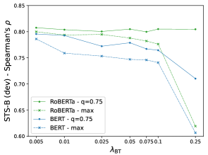
Figure 1: STS-B performances as a function of the $\lambda_{\textrm{BT}}$ coefficient. We show both the max and the upper quartile of the metric distribution after binning by the value of the parameter.

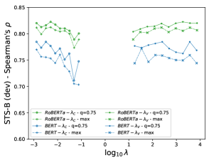
Figure 2: STS-B performances as a function of $\lambda_{\textrm{C}}$ and $\lambda_{\textrm{V}}$. We show both the max and the upper quartile of the metric distribution after binning by the value of the parameter.

A.2 VICReg

The parameter space of VICReg is larger than the one of BT: the loss function depends on 3 parameters $\lambda_{\textrm{V},\textrm{I},\textrm{C}}$. We fix $\lambda_{\textrm{I}}=1$ and scan the remaining two parameters. Since the parameter is larger we use SMAC instead of grid search. Table 3 report the parameters of the scan. Similarly to BT augmentations are not combined, but for each augmentation we scan learning rate, $\lambda_{\textrm{V}}$, and $\lambda_{\textrm{C}}$. For each augmentation strategy we run a total of 50 jobs.

Similarly to BT, there is little sensitivity to the learning rate. We find that the scan favors small values of $\lambda_{\textrm{C}}$ and large values of $\lambda_{\textrm{V}}$. The dev set performances as a function of the augmentation are shown in Tab. 1.

Appendix B Alignment and uniformity

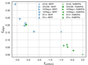
Figure 3: Alignment and uniformity numbers for the models reported in Tab. 6. [CLS]-(Ro)BERT(a) represent text embedding models obtained by using the last layer [CLS] token as the embedding. Lower values are better for both metrics.

We calculate the alignment and uniformity metrics Wang and Isola (2020) for the unsupervised models shown in Tab. 6. Optimizing the unsupervised objective, either sample or dimension contrastive, improve uniformity in all cases while it typically degrades alignment. We notice that these effects are particularly pronounced for the sample contrastive objective optimized by SimCSE, in particular in terms of the improvement in uniformity.

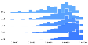
(a) RoBERTa [CLS]

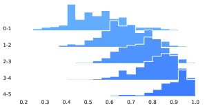
(b) SimCSE RoBERTa

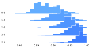
(c) Barlow Twins dropout RoBERTa

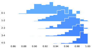
(d) VICReg shuffle RoBERTa

Figure 4: Histograms of cosine similarity between pairs of sentences from the STS-B test set computed with different RoBERTa models, vertically divided in groups according to human ratings of similarity. Notice the different scale of the horizontal axis.

For both BT and VICReg, and in particular for RoBERTa, uniformity improves only marginally through training. However this does not seem to hurt performances on downstream tasks as shown in Tab. 6. This is consistent with the discussion of Huang et al. (2023).

Another representation of this fact is Fig. 4 which shows the distribution of cosine similarities of sentence pairs on the STS-B test set stratified by the similarity rating assigned by human annotators. We see that both SimCSE, BT, and VICReg training increase the divergence of the distributions across buckets, but SimCSE tends, on average, to achieve that by spreading the embeddings apart on the hypersphere (notice the different horizontal scale of the 3 bottom panels in Fig. 4)

Appendix C MTEB

The MTEB (Massive Text Embedding Benchmark) Muennighoff et al. (2023) is a comprehensive evaluation tool designed to assess the performance of text embedding models. It includes well established benchmarks, and spans a wide range of tasks and domains.

We report results on the 56 English language datasets. They are divided in the following tasks (associated evaluation metrics in parenthesis): Classification (accuracy), Clustering (v-measure), Pair Classification (average precision), Rerank (MAP), Retrieval (nDCG@10), STS (Spearman correlation), and Summarization (Spearman correlation). A breadkdown of all datasets, compiled with results from our RoBERTa models, is shown in Tab. 4.

Dataset	SimCSE	VICReg	VICReg	Barlow Twins	Barlow Twins	Barlow Twins	Barlow Twins
		(dropout)	(shuffle)	(dropout)	(shuffle)	(NLI)	(WikiAuto)
Class.
AmazonCounterfactualClassification  O’Neill et al. (2021)	65.5	64.2	65.2	65.0	64.1	60.9	60.5
AmazonPolarityClassification  McAuley and Leskovec (2013)	76.6	63.3	64.6	72.9	62.9	62.7	62.1
AmazonReviewsClassification  McAuley and Leskovec (2013)	35.0	29.0	29.8	33.1	28.7	28.8	30.4
Banking77Classification  Casanueva et al. (2020)	78.1	77.3	76.9	77.9	76.1	75.6	67.6
EmotionClassification  Saravia et al. (2018)	46.8	42.9	44.3	44.5	46.0	42.7	40.5
ImdbClassification  Maas et al. (2011)	73.5	64.9	65.0	72.0	62.4	63.0	57.4
MassiveIntentClassification  FitzGerald et al. (2022)	61.5	61.1	64.7	64.8	57.6	60.5	58.8
MassiveScenarioClassification  FitzGerald et al. (2022)	69.4	70.0	73.6	73.7	62.0	70.9	69.5
MTOPDomainClassification  Li et al. (2021)	85.1	85.9	88.1	88.0	80.9	84.4	81.4
MTOPIntentClassification  Li et al. (2021)	61.3	59.8	64.8	68.3	59.0	56.0	51.0
ToxicConversationsClassification  (url)	68.6	66.4	66.8	69.9	64.2	66.3	66.5
TweetSentimentExtractionClassification (url)	54.0	50.4	51.8	52.4	48.9	51.3	51.6
Clust.
ArxivClusteringP2P♢	32.9	34.9	33.7	35.2	33.1	38.6	33.5
ArxivClusteringS2S♢	21.4	21.8	23.5	23.0	17.9	25.8	23.6
BiorxivClusteringP2P♢	30.1	31.5	30.4	31.7	30.8	36.0	30.0
BiorxivClusteringS2S♢	22.1	22.9	24.6	23.9	16.1	26.1	22.0
MedrxivClusteringP2P♢	26.9	29.0	27.4	28.5	28.8	31.2	28.0
MedrxivClusteringS2S♢	24.9	25.4	26.0	26.0	21.3	28.3	25.6
RedditClustering  Geigle et al. (2021)	33.9	40.1	35.0	41.2	28.7	47.0	41.7
RedditClusteringP2P♢	47.2	48.8	43.1	50.4	46.3	52.5	46.9
StackExchangeClustering  Geigle et al. (2021)	46.3	48.2	49.3	50.9	38.0	51.9	49.1
StackExchangeClusteringP2P♢	29.5	30.7	30.0	30.0	28.5	30.5	33.1
TwentyNewsgroupsClustering  (url)	23.8	33.5	33.1	31.9	19.4	37.2	34.8
PairClass.
SprintDuplicateQuestions  Shah et al. (2018)	86.4	70.7	77.1	74.1	88.5	84.2	84.2
TwitterSemEval2015  Xu et al. (2015)	56.8	56.3	56.3	59.1	51.8	51.3	43.6
TwitterURLCorpus  Lan et al. (2017)	80.4	77.6	78.8	78.8	78.9	78.3	75.4
Rerank.
AskUbuntuDupQuestions  (url)	53.3	51.7	51.9	52.5	51.9	52.2	50.4
MindSmallReranking  Wu et al. (2020)	29.4	29.2	30.3	29.6	27.9	30.0	31.1
SciDocsRR  Cohan et al. (2020)	66.9	65.5	68.7	67.5	62.0	69.7	66.0
StackOverflowDupQuestions  Liu et al. (2018)	39.8	38.1	38.2	39.6	39.5	38.4	34.8
Retr.♠
ArguAna	34.7	43.8	42.6	43.9	35.6	44.1	40.6
ClimateFEVER	14.5	12.8	13.0	19.2	14.2	18.2	22.0
CQADupstackRetrieval	20.4	13.9	17	20.0	18.7	19.4	18.3
DBPedia	15.7	12.0	13.2	15.2	12.8	17.6	17.2
FEVER	28.4	12.6	15.9	28.4	17.1	25.2	33.7
FiQA2018	12.6	11.6	11.3	14.4	10.3	16.1	11.3
HotpotQA	31.4	16.5	16.8	25.0	29.7	26.7	36.2
MSMARCO	8.8	5.4	6.1	7.8	7.8	8.6	12.6
NFCorpus	14.3	9.1	10.6	11.7	10.1	15.6	18.7
NQ	12.3	7.3	8.9	13.6	9.0	12.3	15.4
QuoraRetrieval	80.4	78.5	79.5	79.6	78.3	78.2	75.0
SCIDOCS	6.9	5.7	6.6	7.4	7.2	10.5	9.5
SciFact	34.1	27.3	24.3	25.6	34.7	35.2	34.5
Touche2020	10.9	10.4	9.7	11.9	10.6	13.1	10.5
TRECCOVID	28	30.9	35.1	38.0	26.1	36.7	33.6
STS
BIOSSES (url)	67.7	51.1	56.9	56.9	69.5	58.8	68.6
SICK-R Agirre et al. (2014)	68.9	67.9	70.1	70.6	64.8	64.3	67.4
STS12♡	70.2	64.2	63.2	62.5	65.4	66.5	66.3
STS13♡	81.8	78.7	77.3	77.6	77.7	77.3	77.2
STS14♡	73.2	68.1	66.6	68.1	70.5	67.7	67.4
STS15♡	81.4	78.5	76.3	76.2	80.4	75.3	74.1
STS16♡	80.7	77.5	77.4	79.3	76.0	75.0	74.7
STS17♡	81.8	81.2	81.6	82.0	80.8	78.2	79.8
STS22♡	57.7	60.2	59.8	61.0	60.8	61.9	55.5
STSBenchmark♡	80.1	78.0	76.9	76.6	75.6	75.1	75.2
Summ.
SummEval  Fabbri et al. (2020)	27.6	28.7	29.2	28.9	27.6	27.5	31.1

Table 4: MTEB performances of RoBERTa models on all English datasets grouped by task. We display the scores for both dropout and shuffle augmentations with overall best scores in bold. We also include scores from best Barlow Twins models trained on alternative datasets underlying best scores. $\diamondsuit$: custom clustering datasets created for MTEB, for details we refer to Muennighoff et al. (2023). $\spadesuit$: retrieval datasets are a subset of the BEIR benchmark Thakur et al. (2021). $\heartsuit$: tasks from the original STS benchmark Agirre et al. (2012, 2013).

References

- Abe et al. (2022) Kaori Abe, Sho Yokoi, Tomoyuki Kajiwara, and Kentaro Inui. 2022. Why is sentence similarity benchmark not predictive of application-oriented task performance? In Proceedings of the 3rd Workshop on Evaluation and Comparison of NLP Systems, pages 70–87, Online. Association for Computational Linguistics.
- Agirre et al. (2014) Eneko Agirre, Carmen Banea, Claire Cardie, Daniel M Cer, Mona T Diab, Aitor Gonzalez-Agirre, Weiwei Guo, Rada Mihalcea, German Rigau, and Janyce Wiebe. 2014. Semeval-2014 task 10: Multilingual semantic textual similarity. In SemEval@ COLING, pages 81–91.
- Agirre et al. (2012) Eneko Agirre, Daniel Cer, Mona Diab, and Aitor Gonzalez-Agirre. 2012. Semeval-2012 task 6: A pilot on semantic textual similarity. In * SEM 2012: The First Joint Conference on Lexical and Computational Semantics–Volume 1: Proceedings of the main conference and the shared task, and Volume 2: Proceedings of the Sixth International Workshop on Semantic Evaluation (SemEval 2012), pages 385–393.
- Agirre et al. (2013) Eneko Agirre, Daniel Cer, Mona Diab, Aitor Gonzalez-Agirre, and Weiwei Guo. 2013. * sem 2013 shared task: Semantic textual similarity. In Second joint conference on lexical and computational semantics (* SEM), volume 1: proceedings of the Main conference and the shared task: semantic textual similarity, pages 32–43.
- Balestriero and LeCun (2022) Randall Balestriero and Yann LeCun. 2022. Contrastive and non-contrastive self-supervised learning recover global and local spectral embedding methods. In Advances in Neural Information Processing Systems, volume 35, pages 26671–26685. Curran Associates, Inc.
- Bardes et al. (2022) Adrien Bardes, Jean Ponce, and Yann LeCun. 2022. Vicreg: Variance-invariance-covariance regularization for self-supervised learning.
- Bowman et al. (2015a) Samuel R. Bowman, Gabor Angeli, Christopher Potts, and Christopher D. Manning. 2015a. A large annotated corpus for learning natural language inference. In Proceedings of the 2015 Conference on Empirical Methods in Natural Language Processing, pages 632–642, Lisbon, Portugal. Association for Computational Linguistics.
- Bowman et al. (2015b) Samuel R. Bowman, Gabor Angeli, Christopher Potts, and Christopher D. Manning. 2015b. A large annotated corpus for learning natural language inference. In Proceedings of the 2015 Conference on Empirical Methods in Natural Language Processing, pages 632–642, Lisbon, Portugal. Association for Computational Linguistics.
- Casanueva et al. (2020) Iñigo Casanueva, Tadas Temčinas, Daniela Gerz, Matthew Henderson, and Ivan Vulić. 2020. Efficient intent detection with dual sentence encoders.
- Cer et al. (2017) Daniel Cer, Mona Diab, Eneko Agirre, Inigo Lopez-Gazpio, and Lucia Specia. 2017. SemEval-2017 task 1: Semantic textual similarity multilingual and crosslingual focused evaluation. In Proceedings of the 11th International Workshop on Semantic Evaluation (SemEval-2017). Association for Computational Linguistics.
- Chopra et al. (2005) S. Chopra, R. Hadsell, and Y. LeCun. 2005. Learning a similarity metric discriminatively, with application to face verification. In 2005 IEEE Computer Society Conference on Computer Vision and Pattern Recognition (CVPR’05), volume 1, pages 539–546 vol. 1.
- Chuang et al. (2022) Yung-Sung Chuang, Rumen Dangovski, Hongyin Luo, Yang Zhang, Shiyu Chang, Marin Soljacic, Shang-Wen Li, Scott Yih, Yoon Kim, and James Glass. 2022. DiffCSE: Difference-based contrastive learning for sentence embeddings. In Proceedings of the 2022 Conference of the North American Chapter of the Association for Computational Linguistics: Human Language Technologies, pages 4207–4218, Seattle, United States. Association for Computational Linguistics.
- Cohan et al. (2020) Arman Cohan, Sergey Feldman, Iz Beltagy, Doug Downey, and Daniel S. Weld. 2020. Specter: Document-level representation learning using citation-informed transformers.
- Fabbri et al. (2020) Alexander R. Fabbri, Wojciech Kryściński, Bryan McCann, Caiming Xiong, Richard Socher, and Dragomir Radev. 2020. Summeval: Re-evaluating summarization evaluation.
- Feng et al. (2021) Steven Y. Feng, Varun Gangal, Jason Wei, Sarath Chandar, Soroush Vosoughi, Teruko Mitamura, and Eduard Hovy. 2021. A survey of data augmentation approaches for NLP. In Findings of the Association for Computational Linguistics: ACL-IJCNLP 2021, pages 968–988, Online. Association for Computational Linguistics.
- FitzGerald et al. (2022) Jack FitzGerald, Christopher Hench, Charith Peris, Scott Mackie, Kay Rottmann, Ana Sanchez, Aaron Nash, Liam Urbach, Vishesh Kakarala, Richa Singh, Swetha Ranganath, Laurie Crist, Misha Britan, Wouter Leeuwis, Gokhan Tur, and Prem Natarajan. 2022. Massive: A 1m-example multilingual natural language understanding dataset with 51 typologically-diverse languages.
- Gao et al. (2021) Tianyu Gao, Xingcheng Yao, and Danqi Chen. 2021. SimCSE: Simple contrastive learning of sentence embeddings. In Proceedings of the 2021 Conference on Empirical Methods in Natural Language Processing, pages 6894–6910, Online and Punta Cana, Dominican Republic. Association for Computational Linguistics.
- Garrido et al. (2022) Quentin Garrido, Yubei Chen, Adrien Bardes, Laurent Najman, and Yann Lecun. 2022. On the duality between contrastive and non-contrastive self-supervised learning.
- Geigle et al. (2021) Gregor Geigle, Nils Reimers, Andreas Rücklé, and Iryna Gurevych. 2021. Tweac: Transformer with extendable qa agent classifiers.
- Giorgi et al. (2021) John Giorgi, Osvald Nitski, Bo Wang, and Gary Bader. 2021. DeCLUTR: Deep contrastive learning for unsupervised textual representations. In Proceedings of the 59th Annual Meeting of the Association for Computational Linguistics and the 11th International Joint Conference on Natural Language Processing (Volume 1: Long Papers), pages 879–895, Online. Association for Computational Linguistics.
- Huang et al. (2023) Weiran Huang, Mingyang Yi, Xuyang Zhao, and Zihao Jiang. 2023. Towards the generalization of contrastive self-supervised learning.
- Jiang et al. (2020) Chao Jiang, Mounica Maddela, Wuwei Lan, Yang Zhong, and Wei Xu. 2020. Neural CRF model for sentence alignment in text simplification. In Proceedings of the 58th Annual Meeting of the Association for Computational Linguistics, pages 7943–7960, Online. Association for Computational Linguistics.
- Jiang et al. (2022) Ting Jiang, Jian Jiao, Shaohan Huang, Zihan Zhang, Deqing Wang, Fuzhen Zhuang, Furu Wei, Haizhen Huang, Denvy Deng, and Qi Zhang. 2022. PromptBERT: Improving BERT sentence embeddings with prompts. In Proceedings of the 2022 Conference on Empirical Methods in Natural Language Processing, pages 8826–8837, Abu Dhabi, United Arab Emirates. Association for Computational Linguistics.
- Klein and Nabi (2022) Tassilo Klein and Moin Nabi. 2022. SCD: Self-contrastive decorrelation of sentence embeddings. In Proceedings of the 60th Annual Meeting of the Association for Computational Linguistics (Volume 2: Short Papers), pages 394–400, Dublin, Ireland. Association for Computational Linguistics.
- Lan et al. (2017) Wuwei Lan, Siyu Qiu, Hua He, and Wei Xu. 2017. A continuously growing dataset of sentential paraphrases. In Proceedings of The 2017 Conference on Empirical Methods on Natural Language Processing (EMNLP), pages 1235–1245. Association for Computational Linguistics.
- Li et al. (2021) Haoran Li, Abhinav Arora, Shuohui Chen, Anchit Gupta, Sonal Gupta, and Yashar Mehdad. 2021. MTOP: A comprehensive multilingual task-oriented semantic parsing benchmark. In Proceedings of the 16th Conference of the European Chapter of the Association for Computational Linguistics: Main Volume, pages 2950–2962, Online. Association for Computational Linguistics.
- Liu et al. (2018) Xueqing Liu, Chi Wang, Yue Leng, and ChengXiang Zhai. 2018. Linkso: a dataset for learning to retrieve similar question answer pairs on software development forums. In Proceedings of the 4th ACM SIGSOFT International Workshop on NLP for Software Engineering, pages 2–5.
- Maas et al. (2011) Andrew L. Maas, Raymond E. Daly, Peter T. Pham, Dan Huang, Andrew Y. Ng, and Christopher Potts. 2011. Learning word vectors for sentiment analysis. In Proceedings of the 49th Annual Meeting of the Association for Computational Linguistics: Human Language Technologies, pages 142–150, Portland, Oregon, USA. Association for Computational Linguistics.
- McAuley and Leskovec (2013) Julian McAuley and Jure Leskovec. 2013. Hidden factors and hidden topics: Understanding rating dimensions with review text. In Proceedings of the 7th ACM Conference on Recommender Systems, RecSys ’13, page 165–172, New York, NY, USA. Association for Computing Machinery.
- Muennighoff (2022) Niklas Muennighoff. 2022. Sgpt: Gpt sentence embeddings for semantic search.
- Muennighoff et al. (2023) Niklas Muennighoff, Nouamane Tazi, Loic Magne, and Nils Reimers. 2023. MTEB: Massive text embedding benchmark. In Proceedings of the 17th Conference of the European Chapter of the Association for Computational Linguistics, pages 2014–2037, Dubrovnik, Croatia. Association for Computational Linguistics.
- Ni et al. (2022a) Jianmo Ni, Gustavo Hernandez Abrego, Noah Constant, Ji Ma, Keith Hall, Daniel Cer, and Yinfei Yang. 2022a. Sentence-t5: Scalable sentence encoders from pre-trained text-to-text models. In Findings of the Association for Computational Linguistics: ACL 2022, pages 1864–1874, Dublin, Ireland. Association for Computational Linguistics.
- Ni et al. (2022b) Jianmo Ni, Chen Qu, Jing Lu, Zhuyun Dai, Gustavo Hernandez Abrego, Ji Ma, Vincent Zhao, Yi Luan, Keith Hall, Ming-Wei Chang, and Yinfei Yang. 2022b. Large dual encoders are generalizable retrievers. In Proceedings of the 2022 Conference on Empirical Methods in Natural Language Processing, pages 9844–9855, Abu Dhabi, United Arab Emirates. Association for Computational Linguistics.
- O’Neill et al. (2021) James O’Neill, Polina Rozenshtein, Ryuichi Kiryo, Motoko Kubota, and Danushka Bollegala. 2021. I wish i would have loved this one, but i didn’t – a multilingual dataset for counterfactual detection in product reviews.
- Reimers et al. (2016) Nils Reimers, Philip Beyer, and Iryna Gurevych. 2016. Task-oriented intrinsic evaluation of semantic textual similarity. In Proceedings of COLING 2016, the 26th International Conference on Computational Linguistics: Technical Papers, pages 87–96, Osaka, Japan. The COLING 2016 Organizing Committee.
- Reimers and Gurevych (2019) Nils Reimers and Iryna Gurevych. 2019. Sentence-BERT: Sentence embeddings using Siamese BERT-networks. In Proceedings of the 2019 Conference on Empirical Methods in Natural Language Processing and the 9th International Joint Conference on Natural Language Processing (EMNLP-IJCNLP), pages 3982–3992, Hong Kong, China. Association for Computational Linguistics.
- Saravia et al. (2018) Elvis Saravia, Hsien-Chi Toby Liu, Yen-Hao Huang, Junlin Wu, and Yi-Shin Chen. 2018. CARER: Contextualized affect representations for emotion recognition. In Proceedings of the 2018 Conference on Empirical Methods in Natural Language Processing, pages 3687–3697, Brussels, Belgium. Association for Computational Linguistics.
- Shah et al. (2018) Darsh Shah, Tao Lei, Alessandro Moschitti, Salvatore Romeo, and Preslav Nakov. 2018. Adversarial domain adaptation for duplicate question detection. In Proceedings of the 2018 Conference on Empirical Methods in Natural Language Processing, pages 1056–1063, Brussels, Belgium. Association for Computational Linguistics.
- Shwartz-Ziv et al. (2022) Ravid Shwartz-Ziv, Randall Balestriero, and Yann LeCun. 2022. What do we maximize in self-supervised learning?
- Su et al. (2022) Hongjin Su, Weijia Shi, Jungo Kasai, Yizhong Wang, Yushi Hu, Mari Ostendorf, Wen tau Yih, Noah A. Smith, Luke Zettlemoyer, and Tao Yu. 2022. One embedder, any task: Instruction-finetuned text embeddings.
- Thakur et al. (2021) Nandan Thakur, Nils Reimers, Andreas Rücklé, Abhishek Srivastava, and Iryna Gurevych. 2021. Beir: A heterogenous benchmark for zero-shot evaluation of information retrieval models.
- van den Oord et al. (2019) Aaron van den Oord, Yazhe Li, and Oriol Vinyals. 2019. Representation learning with contrastive predictive coding.
- Wang et al. (2021) Kexin Wang, Nils Reimers, and Iryna Gurevych. 2021. TSDAE: Using transformer-based sequential denoising auto-encoderfor unsupervised sentence embedding learning. In Findings of the Association for Computational Linguistics: EMNLP 2021, pages 671–688, Punta Cana, Dominican Republic. Association for Computational Linguistics.
- Wang et al. (2022) Liang Wang, Nan Yang, Xiaolong Huang, Binxing Jiao, Linjun Yang, Daxin Jiang, Rangan Majumder, and Furu Wei. 2022. Text embeddings by weakly-supervised contrastive pre-training.
- Wang and Isola (2020) Tongzhou Wang and Phillip Isola. 2020. Understanding contrastive representation learning through alignment and uniformity on the hypersphere. In Proceedings of the 37th International Conference on Machine Learning, ICML’20. JMLR.org.
- Wei and Zou (2019) Jason Wei and Kai Zou. 2019. EDA: Easy data augmentation techniques for boosting performance on text classification tasks. In Proceedings of the 2019 Conference on Empirical Methods in Natural Language Processing and the 9th International Joint Conference on Natural Language Processing (EMNLP-IJCNLP), pages 6382–6388, Hong Kong, China. Association for Computational Linguistics.
- Williams et al. (2018a) Adina Williams, Nikita Nangia, and Samuel Bowman. 2018a. A broad-coverage challenge corpus for sentence understanding through inference. In Proceedings of the 2018 Conference of the North American Chapter of the Association for Computational Linguistics: Human Language Technologies, Volume 1 (Long Papers), pages 1112–1122, New Orleans, Louisiana. Association for Computational Linguistics.
- Williams et al. (2018b) Adina Williams, Nikita Nangia, and Samuel Bowman. 2018b. A broad-coverage challenge corpus for sentence understanding through inference. In Proceedings of the 2018 Conference of the North American Chapter of the Association for Computational Linguistics: Human Language Technologies, Volume 1 (Long Papers), pages 1112–1122, New Orleans, Louisiana. Association for Computational Linguistics.
- Wu et al. (2020) Fangzhao Wu, Ying Qiao, Jiun-Hung Chen, Chuhan Wu, Tao Qi, Jianxun Lian, Danyang Liu, Xing Xie, Jianfeng Gao, Winnie Wu, et al. 2020. Mind: A large-scale dataset for news recommendation. In Proceedings of the 58th Annual Meeting of the Association for Computational Linguistics, pages 3597–3606.
- Wu et al. (2022) Xing Wu, Chaochen Gao, Zijia Lin, Jizhong Han, Zhongyuan Wang, and Songlin Hu. 2022. InfoCSE: Information-aggregated contrastive learning of sentence embeddings. In Findings of the Association for Computational Linguistics: EMNLP 2022, pages 3060–3070, Abu Dhabi, United Arab Emirates. Association for Computational Linguistics.
- Xu et al. (2023) Jiahao Xu, Wei Shao, Lihui Chen, and Lemao Liu. 2023. Imsimcse: Improving contrastive learning for sentence embeddings from two perspectives.
- Xu et al. (2015) Wei Xu, Chris Callison-Burch, and William B Dolan. 2015. Semeval-2015 task 1: Paraphrase and semantic similarity in twitter (pit). In Proceedings of the 9th international workshop on semantic evaluation (SemEval 2015), pages 1–11.
- Zbontar et al. (2021) Jure Zbontar, Li Jing, Ishan Misra, Yann LeCun, and Stéphane Deny. 2021. Barlow twins: Self-supervised learning via redundancy reduction.
- Zhang et al. (2020) Yan Zhang, Ruidan He, Zuozhu Liu, Kwan Hui Lim, and Lidong Bing. 2020. An unsupervised sentence embedding method by mutual information maximization. In Proceedings of the 2020 Conference on Empirical Methods in Natural Language Processing (EMNLP), pages 1601–1610, Online. Association for Computational Linguistics.