Improved Standard-Model prediction for $\boldsymbol{K_{L}\to\ell^{+}\ell^{-}}$

Abstract

We present a comprehensive calculation of the $K_{L}\to\gamma^{*}\gamma^{*}$ form factor in dispersion theory, using input from the leptonic decays $K_{L}\to\ell^{+}\ell^{-}\gamma$, $K_{L}\to\ell_{1}^{+}\ell_{1}^{-}\ell_{2}^{+}\ell_{2}^{-}$, the hadronic mode $K_{L}\to\pi^{+}\pi^{-}\gamma$, the normalization $K_{L}\to\gamma\gamma$, and the matching to asymptotic constraints. As key result we obtain an improved determination of the long-distance contribution to $K_{L}\to\ell^{+}\ell^{-}$, leading to the Standard-Model predictions $\text{Br}[K_{L}\to\mu^{+}\mu^{-}]=7.44^{+0.41}_{-0.34}\times 10^{-9}$, $\text{Br}[K_{L}\to e^{+}e^{-}]=8.46(37)\times 10^{-12}$, and more stringent limits on physics beyond the Standard Model. We provide a detailed breakdown of the current uncertainty, and delineate how future experiments and the interplay with lattice QCD could help further improve the precision.

1 Introduction

Rare kaon decays are sensitive low-energy probes of physics beyond the Standard Model (BSM) Cirigliano et al. (2012). Next to the neutrino modes $K^{+}\to\pi^{+}\nu\bar{\nu}$ Cortina Gil et al. (2021) and $K_{L}\to\pi^{0}\nu\bar{\nu}$ Ahn et al. (2019), another promising channel concerns the decay of a neutral kaon into a dilepton pair, whose short-distance (SD) properties differ markedly for the $K_{S}$ and $K_{L}$ channels. The general decomposition of the amplitude

$$\mathcal{A}\big{[}K\to\ell^{+}(p_{1})\ell^{-}(p_{2})\big{]}=\bar{u}(p_{2})\big{[}iB+C\gamma_{5}\big{]}v(p_{1})$$ (1)

leads to a decay width

$$\Gamma\big{[}K\to\ell^{+}\ell^{-}\big{]}=\frac{M_{K}}{8\pi}\sigma_{\ell}(M_{K}^{2})\big{[}(\sigma_{\ell}(M_{K}^{2}))^{2}|B|^{2}+|C|^{2}\big{]},\qquad\sigma_{\ell}(M_{K}^{2})=\sqrt{1-\frac{4m_{\ell}^{2}}{M_{K}^{2}}}.$$ (2)

For $K_{S}\to\ell^{+}\ell^{-}$ the dominant contribution arises from the long-distance (LD) $K_{S}\to\gamma^{*}\gamma^{*}\to\ell^{+}\ell^{-}$ $P$-wave amplitude $B$ D’Ambrosio and Espriu (1986); Ecker and Pich (1991), which, due to the absence of $CP$-invariant local contributions at two-loop order in chiral perturbation theory (ChPT) can be predicted with reasonable accuracy Ecker and Pich (1991)

$$\text{Br}[K_{S}\to\mu^{+}\mu^{-}]\big{|}_{\text{LD}}\simeq 5.0(3)\times 10^{-12},\qquad\text{Br}[K_{S}\to e^{+}e^{-}]\big{|}_{\text{LD}}\simeq 2.1(1)\times 10^{-14},$$ (3)

where the uncertainty is propagated from $\text{Br}[K_{S}\to\gamma\gamma]=2.63(17)\times 10^{-6}$ Workman et al. (2022); Ambrosino et al. (2008); Lai et al. (2003a), but does not include theory uncertainties in $\text{Br}[K_{S}\to\ell^{+}\ell^{-}]/\text{Br}[K_{S}\to\gamma\gamma]$ itself. Current limits Aaij et al. (2020); Ambrosino et al. (2009)

$$\text{Br}[K_{S}\to\mu^{+}\mu^{-}]<2.1\times 10^{-10},\qquad\text{Br}[K_{S}\to e^{+}e^{-}]<9\times 10^{-9},$$ (4)

are less than two orders of magnitude away for the muon mode, while the electron channel appears out of reach for the foreseeable future. In this process, a $CP$-violating SD contribution occurs via the $S$-wave amplitude $C$, at the level of $\text{Br}[K_{S}\to\mu^{+}\mu^{-}]\big{|}_{\text{SD}}\simeq 1.7(2)\times 10^{-13}$ Buchalla et al. (1996); Isidori and Unterdorfer (2004); Cirigliano et al. (2012); Brod and Stamou (2023). A first step towards an improved calculation of $\pi\pi$ rescattering effects in the LD SM contribution was taken in Ref. Colangelo et al. (2016) (in terms of partial waves for $\gamma^{*}\gamma^{*}\to\pi\pi$ García-Martín and Moussallam (2010); Hoferichter et al. (2011); Moussallam (2013); Danilkin and Vanderhaeghen (2019); Hoferichter and Stoffer (2019); Danilkin et al. (2020)), which would allow one to reduce the hidden uncertainty in Eq. (3) due to higher orders in ChPT D’Ambrosio et al. (2022).

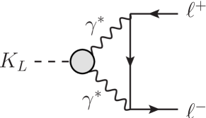
Figure 1: LD contribution to $K_{L}\to\ell^{+}\ell^{-}$. The gray blob refers to the $K_{L}\to\gamma^{*}\gamma^{*}$ transition form factor.

For $K_{L}\to\ell^{+}\ell^{-}$ the roles become reversed, and the $CP$-conserving LD contribution now proceeds via the $C$ amplitude in Eq. (1). Normalizing to the $K_{L}\to\gamma\gamma$ decay, the decay rate can be written as

$$R_{L}^{\ell}=\frac{\text{Br}[K_{L}\to\ell^{+}\ell^{-}]}{\text{Br}[K_{L}\to\gamma\gamma]}=2\sigma_{\ell}(M_{K}^{2})\bigg{(}\frac{\alpha}{\pi}r_{\ell}\bigg{)}^{2}\big{|}\mathcal{A}_{\ell}(M_{K}^{2})\big{|}^{2},\qquad r_{\ell}=\frac{m_{\ell}}{M_{K}},\qquad\alpha=\frac{e^{2}}{4\pi},$$ (5)

where the dominant imaginary part comes from $\gamma\gamma$ intermediate states Martin et al. (1970)

$$\text{Im}_{\gamma\gamma}\mathcal{A}_{\ell}(M_{K}^{2})=\frac{\pi}{2\sigma_{\ell}(M_{K}^{2})}\log\big{[}y_{\ell}(M_{K}^{2})\big{]},\qquad y_{\ell}(M_{K}^{2})=\frac{1-\sigma_{\ell}(M_{K}^{2})}{1+\sigma_{\ell}(M_{K}^{2})}.$$ (6)

The real part is typically decomposed into the loop function that corresponds to the one-loop result in ChPT and a local contribution $\chi(\mu)$ Gómez Dumm and Pich (1998); Knecht et al. (1999); Isidori and Unterdorfer (2004)

$$\text{Re}\,\mathcal{A}_{\ell}(M_{K}^{2})=\frac{1}{\sigma_{\ell}(M_{K}^{2})}\bigg{[}\text{Li}_{2}\big{[}-y_{\ell}(M_{K}^{2})\big{]}+\frac{1}{4}\log^{2}\big{[}y_{\ell}(M_{K}^{2})\big{]}+\frac{\pi^{2}}{12}\bigg{]}+3\log\frac{m_{\ell}}{\mu}-\frac{5}{2}+\chi(\mu),$$ (7)

where $\chi(\mu)$ receives both LD and SD contributions in the SM, see Figs. 1 and 2. Fixing the sign following the arguments from Refs. Pich and de Rafael (1996); Gómez Dumm and Pich (1998); Isidori and Unterdorfer (2004), the SD part is known to about $4\%$ precision Buchalla and Buras (1994); Gorbahn and Haisch (2006)

$$\chi_{\text{SD}}^{\text{SM}}=-1.80(6),$$ (8)

see App. A, with uncertainties dominated by CKM matrix elements. The experimental results Workman et al. (2022); Ambrose et al. (2000); Akagi et al. (1995); Heinson et al. (1995); Ambrose et al. (1998)

$$\text{Br}[K_{L}\to\mu^{+}\mu^{-}]=6.84(11)\times 10^{-9},\qquad\text{Br}[K_{L}\to e^{+}e^{-}]=8.7^{+5.7}_{-4.1}\times 10^{-12},$$ (9)

or, using $\text{Br}[K_{L}\to\gamma\gamma]=5.47(4)\times 10^{-4}$ Workman et al. (2022),

$$R_{L}^{\mu}=1.250(24)\times 10^{-5},\qquad R_{L}^{e}=1.59^{+1.04}_{-0.75}\times 10^{-8},$$ (10)

would thus allow one to derive BSM constraints if the LD contribution to $\chi(\mu)$ could be calculated.

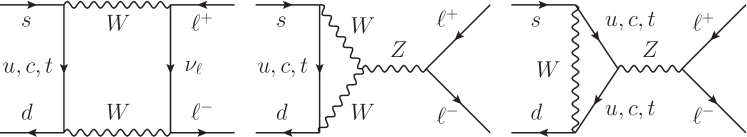
Figure 2: SD contributions to $K_{L}\to\ell^{+}\ell^{-}$ in the SM.

Previous theoretical estimates of this contribution have relied on ChPT, leading to diagrams including the mixing of the $K_{L}$ to $\pi^{0}$, $\eta$, $\eta^{\prime}$ Gómez Dumm and Pich (1998); Knecht et al. (1999); Greynat and de Rafael (2003), or on parameterizations of the $K_{L}\to\gamma^{*}\gamma^{*}$ form factor informed by the radiative decays $K_{L}\to\ell^{+}\ell^{-}\gamma$ D’Ambrosio et al. (1998); Valencia (1998) and the asymptotic behavior expected from a partonic calculation Isidori and Unterdorfer (2004). More recently, also first steps towards a lattice-QCD calculation of $\chi(\mu)$ have been taken Christ et al. (2023); Zhao and Christ (2022); Christ et al. (2020), and proposals were developed to extract SD information from the time evolution of the $K\to\ell^{+}\ell^{-}$ decay rate D’Ambrosio and Kitahara (2017); Dery et al. (2021, 2023). In view of the experimental prospects for future precision measurements of $K_{L}$ decays in phase 2 of HIKE Cortina Gil et al. (2022) and at KOTO II Nanjo (2023) (see also Ref. Aaij et al. (2022)), it is thus timely to revisit the calculation of the $K_{L}\to\gamma^{*}\gamma^{*}$ form factor using methods that were recently developed in the context of pseudoscalar-pole contributions to hadronic light-by-light scattering in the anomalous magnetic moment of the muon Aoyama et al. (2020); Colangelo et al. (2014a, b, 2015); Hoferichter et al. (2018a, b).

To this end, we analyze the $K_{L}\to\gamma^{*}\gamma^{*}$ form factor in dispersion theory, which allows us to not only include the leptonic modes $K_{L}\to\ell^{+}\ell^{-}\gamma$, $K_{L}\to\ell_{1}^{+}\ell_{1}^{-}\ell_{2}^{+}\ell_{2}^{-}$ in its reconstruction from data, but, crucially, also the hadronic channel $K_{L}\to\pi^{+}\pi^{-}\gamma$. In addition, we perform the matching to asymptotic constraints via a dispersive representation of the respective loop integrals, which allows for a better separation of their low- and high-energy components. This strategy follows closely our calculation of the $\pi^{0}\to\gamma^{*}\gamma^{*}$ transition form factor Schneider et al. (2012); Hoferichter et al. (2012, 2014a, 2018a, 2018b), which was mainly motivated by the pion-pole contribution to hadronic light-by-light scattering, but later applied also to specific channels in hadronic vacuum polarization Hoferichter et al. (2019); Hoid et al. (2020); Hoferichter et al. (2023a, b) and, most importantly in the context of $K_{L}\to\ell^{+}\ell^{-}$, to an improved SM prediction for $\pi^{0}\to e^{+}e^{-}$ Hoferichter et al. (2022). In addition, the calculation presented here profits from the experience gained with the analog form factors in $\eta,\eta^{\prime}\to\gamma^{*}\gamma^{*}$ Hanhart et al. (2013); Holz et al. (2021); Kubis and Plenter (2015); Holz et al. (2022) and $f_{1}\to\gamma^{*}\gamma^{*}$ Hoferichter and Stoffer (2020); Zanke et al. (2021); Hoferichter et al. (2023c).

The outline of our analysis is as follows. We first derive a dispersive representation of $K_{L}\to\gamma^{*}\gamma^{*}$ in Sec. 2, which is then matched to asymptotic constraints in Sec. 3 to arrive at the final representation given in Sec. 4. The resulting SM prediction for $K_{L}\to\ell^{+}\ell^{-}$ is derived in Sec. 5, leading to the BSM constraints discussed in Sec. 6, before concluding in Sec. 7. Details of the SD contribution in the SM, the dispersive representation of the loop integrals, and the integration kernels for $K_{L}\to\ell^{+}\ell^{-}$ are discussed in the appendices.

2 Dispersive calculation of $\boldsymbol{K_{L}\to\gamma^{*}\gamma^{*}}$

2.1 Leptonic processes

Following the conventions of Ref. Cirigliano et al. (2012), the amplitude for $K_{L}\to\gamma^{*}\gamma^{*}$ can be written as

$$\mathcal{A}^{\mu\nu}[K_{L}\to\gamma^{*}(q_{1},\mu)\gamma^{*}(q_{2},\nu)]=i\epsilon^{\mu\nu\alpha\beta}q_{1\alpha}q_{2\beta}c(q_{1}^{2},q_{2}^{2}),$$ (11)

since the other two Lorentz structures, associated with scalar amplitudes $a(q_{1}^{2},q_{2}^{2})$, $b(q_{1}^{2},q_{2}^{2})$, only lead to $CP$-violating contributions. Accordingly, the scalar function $c(q_{1}^{2},q_{2}^{2})$ defines the $K_{L}\to\gamma^{*}\gamma^{*}$ transition form factor of primary interest to us. Its normalization is determined via the on-shell process

$$\Gamma_{\gamma\gamma}\equiv\Gamma[K_{L}\to\gamma\gamma]=\frac{M_{K}^{3}}{64\pi}\big{|}c(0,0)\big{|}^{2}.$$ (12)

The spectrum for the singly-virtual decays $K_{L}\to\ell^{+}\ell^{-}\gamma$ reads

$$\frac{1}{\Gamma_{\gamma\gamma}}\frac{d\Gamma_{\ell}}{dz}=\frac{2}{z}(1-z)^{3}\frac{1}{\pi}\text{Im}\,\Pi_{\ell}(z)|f(z)|^{2},$$ (13)

with $z=q^{2}/M_{K}^{2}$, $q^{2}$ the virtuality of the dilepton pair, $f(z)=c(q^{2},0)/c(0,0)$, and spectral function

$$\frac{1}{\pi}\text{Im}\,\Pi_{\ell}(z)=\theta\big{(}z-4r_{\ell}^{2}\big{)}\frac{\alpha}{3\pi}\bigg{(}1+2\frac{r_{\ell}^{2}}{z}\bigg{)}\sqrt{1-\frac{4r_{\ell}^{2}}{z}}.$$ (14)

Similarly, the doubly-virtual process $K_{L}\to\ell_{1}^{+}\ell_{1}^{-}\ell_{2}^{+}\ell_{2}^{-}$ is sensitive to the normalized form factor $f(z_{1},z_{2})=c(q_{1}^{2},q_{2}^{2})/c(0,0)$, according to

$$\frac{1}{\Gamma_{\gamma\gamma}}\frac{d^{2}\Gamma_{\ell_{1}\ell_{2}}}{dz_{1}dz_{2}}=\frac{2}{z_{1}z_{2}}\lambda^{3/2}(1,z_{1},z_{2})\frac{1}{\pi}\text{Im}\,\Pi_{\ell_{1}}(z_{1})\frac{1}{\pi}\text{Im}\,\Pi_{\ell_{2}}(z_{2})|f(z_{1},z_{2})|^{2},$$ (15)

where $\lambda(a,b,c)=a^{2}+b^{2}+c^{2}-2(ab+ac+bc)$. However, because of the kinematic constraints and statistics of these decays, both processes can, in practice, only provide useful information about the slope parameter $b_{K_{L}}$ defined as

$$\frac{c(q^{2},0)}{c(0,0)}=1+b_{K_{L}}q^{2}+\mathcal{O}(q^{4}).$$ (16)

Among the two popular parameterizations of the form factor, Bergström, Massó, and Singer (BMS) have proposed Sarraga and Munczek (1971); Bergström et al. (1983)

$$f_{\text{BMS}}(z)=\frac{M_{\rho}^{2}}{M_{\rho}^{2}-zM_{K}^{2}}+\alpha_{K^{*}}A_{K^{*}}(z),$$ (17)

where

$$A_{K^{*}}(z)=\frac{C_{K^{*}}M_{K^{*}}^{2}}{M_{K^{*}}^{2}-zM_{K}^{2}}\bigg{[}\bigg{(}1+\frac{\beta_{K^{*}}}{3}\bigg{)}-\frac{M_{\rho}^{2}}{M_{\rho}^{2}-zM_{K}^{2}}-\frac{\beta_{K^{*}}}{3}\bigg{(}\frac{1}{3}\frac{M_{\omega}^{2}}{M_{\omega}^{2}-zM_{K}^{2}}+\frac{2}{3}\frac{M_{\phi}^{2}}{M_{\phi}^{2}-z{M_{K}^{2}}}\bigg{)}\bigg{]},$$ (18)

with $C_{K^{*}}=2.5$ and $\beta_{K^{*}}=1$ for the resulting BMS model Bergström et al. (1983). The form in Eq. (18) is constructed in such a way that $A_{K^{*}}(0)=0$, which reflects the fact that the decay $K\to\pi\gamma$ is not allowed by angular momentum conservation, and thus an on-shell $K^{*}\simeq K\pi\to\gamma$ transition cannot occur either. Phenomenologically, this is an important feature of the $K^{*}$ contribution, as it can be sizable for the slope of the form factor, without altering the normalization. The singly-virtual decays constrain $\alpha_{K^{*}}=-0.217(34)$ (dominated by Ref. Abouzaid et al. (2007)) and $\alpha_{K^{*}}=-0.158(27)$ (dominated by Ref. Alavi-Harati et al. (2001a)), for the electron and muon channel, respectively. There is also a measurement from the doubly-virtual process where $\ell_{1}=\ell_{2}=e$ Alavi-Harati et al. (2001b), which finds $\alpha_{K^{*}}=-0.14(22)$ with a large uncertainty after assuming factorization for the form factor. The world average, $\alpha_{K^{*}}=-0.205(22)$ Workman et al. (2022), then leads to

$$b_{K_{L}}=2.72(11)\,\text{GeV}^{-2}.$$ (19)

Second, D’Ambrosio, Isidori, and Portolés (DIP) have proposed the parameterization D’Ambrosio et al. (1998)

$$f(z_{1},z_{2})=1+\alpha_{\text{DIP}}\sum_{i=1,2}\frac{z_{i}}{z_{i}-M_{\rho}^{2}/M_{K}^{2}}+\beta_{\text{DIP}}\prod_{i=1,2}\frac{z_{i}}{z_{i}-M_{\rho}^{2}/M_{K}^{2}},$$ (20)

often subject to the high-energy constraint $1+2\alpha_{\text{DIP}}+\beta_{\text{DIP}}=0$. In addition to the singly-virtual modes Alavi-Harati et al. (2001a); Abouzaid et al. (2007), the parameter $\alpha_{\text{DIP}}$ was also extracted from the $\ell_{1}=e$, $\ell_{2}=\mu$ channel Alavi-Harati et al. (2003) assuming $\beta_{\text{DIP}}=0$. The global average, $\alpha_{\text{DIP}}=-1.69(8)$ Workman et al. (2022) is dominated by the $K_{L}\to e^{+}e^{-}\gamma$ mode, leading to $b_{K_{L}}=2.81(13)\,\text{GeV}^{-2}$, consistent with the extraction (19) from the BMS model within uncertainties.

Our aim is to improve model parameterizations of $c(q_{1}^{2},q_{2}^{2})$, by developing a dispersive representation for this form factor in analogy to Refs. Hoferichter et al. (2018a, b). In particular, this allows us to profit not only from the leptonic decay data, but also from data on the related hadronic process $K_{L}\to\pi^{+}\pi^{-}\gamma$, to which we turn next.

2.2 $\boldsymbol{K_{L}\to\pi^{+}\pi^{-}\gamma^{*}}$

We decompose the $K_{L}\to\pi^{+}\pi^{-}\gamma^{*}$ amplitude as Ecker et al. (1994); D’Ambrosio and Portolés (1998); Cirigliano et al. (2012)

$$\mathcal{A}^{\mu}[K_{L}(p_{K})\to\pi^{+}(p_{1})\pi^{-}(p_{2})\gamma^{*}(\mu,q)]=\frac{E(z_{i})}{M_{K}}\big{(}z_{1}p_{2}^{\mu}-z_{2}p_{1}^{\mu}\big{)}+\frac{M(z_{i})}{M_{K}^{3}}i\epsilon^{\mu\alpha\beta\gamma}p_{1\alpha}p_{2\beta}q_{\gamma},$$ (21)

where $z_{i}=q\cdot p_{i}/M_{K}^{2}$ and $z_{3}=z_{1}+z_{2}=E_{\gamma}^{*}/M_{K}$, $E_{\gamma}^{*}$ denoting the photon energy in the kaon rest frame. As a first step, we rewrite these conventions in terms of Mandelstam variables Holz et al. (2021); Kubis and Plenter (2015)

$$s=(p_{K}-p_{1})^{2}=(q+p_{2})^{2},\qquad t=(p_{K}-q)^{2}=(p_{1}+p_{2})^{2},\qquad u=(p_{K}-p_{2})^{2}=(q+p_{1})^{2},$$ (22)

with $s+t+u=2M_{\pi}^{2}+M_{K}^{2}+q^{2}$, and the center-of-mass angle

$$\cos\theta_{t}=z_{t}=\frac{s-u}{\sigma_{\pi}(t)\lambda^{1/2}(M_{K}^{2},t,q^{2})},\qquad\sigma_{\pi}(t)=\sqrt{1-\frac{4M_{\pi}^{2}}{t}},$$ (23)

leading to the identifications

$$z_{1}=\frac{u-q^{2}-M_{\pi}^{2}}{2M_{K}^{2}},\qquad z_{2}=\frac{s-q^{2}-M_{\pi}^{2}}{2M_{K}^{2}},\qquad z_{3}=\frac{M_{K}^{2}-t-q^{2}}{2M_{K}^{2}}=\frac{E_{\gamma}^{*}}{M_{K}}.$$ (24)

Moreover, the difference of the $z_{i}$ is related to $z_{t}$ according to

$$z_{t}=\frac{2M_{K}^{2}(z_{1}-z_{2})}{\sigma_{\pi}(t)\lambda^{1/2}(M_{K}^{2},t,q^{2})}.$$ (25)

The two amplitudes are typically decomposed into “inner-bremsstrahlung” (IB) and “direct emission” (DE), where the former only contributes to the electric amplitude $E(z_{i})$

$$E_{\text{IB}}(z_{i})=\frac{e}{z_{1}z_{2}M_{K}}\mathcal{A}[K_{L}\to\pi\pi]\overset{q^{2}\to 0}{\to}\frac{e}{1-\sigma_{\pi}^{2}(t)z_{t}^{2}}\bigg{(}\frac{2M_{K}}{E_{\gamma}^{*}}\bigg{)}^{2}\frac{\mathcal{A}[K_{L}\to\pi\pi]}{M_{K}},$$ (26)

which is thus $CP$ violating, but still significant due to the infrared enhancement. The remaining contribution can be expanded in terms of multipoles

$$E_{\text{DE}}(z_{i}) =E_{1}(z_{3})+E_{2}(z_{3})(z_{1}-z_{2})+\mathcal{O}\big{(}(z_{1}-z_{2})^{2}\big{)},$$

$$M(z_{i}) =M_{1}(z_{3})+M_{2}(z_{3})(z_{1}-z_{2})+\mathcal{O}\big{(}(z_{1}-z_{2})^{2}\big{)},$$ (27)

where the odd electric and even magnetic multipoles are $CP$ violating. This can be contrasted with the expected partial-wave expansion Jacob and Wick (1959), e.g.,

$$M(z_{i})=\sum_{\text{odd }\ell}P_{\ell}^{\prime}(z_{t})M_{\ell}(t),$$ (28)

with derivatives of the Legendre polynomials $P_{\ell}^{\prime}(z)$, so that requiring $CP$ invariance indeed only leaves the odd partial waves in $M(z_{i})$ (and vice versa for $E(z_{i})$). To constrain the $CP$-conserving $K_{L}\to\gamma^{*}\gamma^{*}$ process via the $\pi\pi$ singularities, we are thus mainly interested in the first multipole of $M(z_{i})$, which takes the role of the partial wave $f_{1}(t)$ in Refs. Holz et al. (2021); Kubis and Plenter (2015).

Experimentally, $M_{1}(z_{3})$ was studied in Refs. Ramberg et al. (1993); Alavi-Harati et al. (2001c); Abouzaid et al. (2006) for $q^{2}=0$, using a $\rho$-pole ansatz of the form Lin and Valencia (1988)

$$M=\bar{M}_{1}\bigg{(}1+\frac{a}{M_{\rho}^{2}-M_{K}^{2}+2M_{K}^{2}z_{3}}\bigg{)}=\bar{M}_{1}\bigg{(}1+\frac{a}{M_{\rho}^{2}-t}\bigg{)},\qquad\bar{M}_{1}=\frac{e|f_{S}|}{M_{K}}\tilde{g}_{M_{1}},$$ (29)

with $|\tilde{g}_{M_{1}}|=1.20(9)$, $a=-0.738(19)\,\text{GeV}^{2}$ Abouzaid et al. (2006), and the rest of the normalization was expressed in terms of the $K_{S}\to\pi^{+}\pi^{-}$ decay Sehgal and Wanninger (1992); Sehgal and van Leusen (1999)

$$\Gamma[K_{S}\to\pi^{+}\pi^{-}]=\frac{|f_{S}|^{2}}{16\pi M_{K}}\sigma_{\pi}(M_{K}^{2}).$$ (30)

Assuming no interference with the IB contribution, a branching fraction of $\text{Br}[K_{L}\to\pi^{+}\pi^{-}\gamma\text{ (DE)}]=2.84(11)\times 10^{-5}$ is given in Ref. Workman et al. (2022) (based on the $K_{L}\to\pi^{+}\pi^{-}$ measurement from Ref. Ambrosino et al. (2006) and the ratio of IB vs. DE branching fractions from Refs. Alavi-Harati et al. (2001c); Abouzaid et al. (2006); Ramberg et al. (1993)). Finally, there is a measurement of the branching fraction $\text{Br}[K_{L}\to\pi^{+}\pi^{-}e^{+}e^{-}]=3.08(20)\times 10^{-7}$ Lai et al. (2003b). Apart from branching fractions, experiments also performed analyses of the double differential decay rate

$$\frac{\text{d}\Gamma[K_{L}\to\pi^{+}\pi^{-}\gamma]}{\text{d}E_{\gamma}^{*}\,\text{d}\cos\theta}= \left(\frac{\beta E_{\gamma}^{*}}{8\pi M_{K}}\right)^{3}\left(1-\frac{2E_{\gamma}^{*}}{M_{K}}\right)\sin^{2}\theta\big{(}|E_{\text{IB}}+E_{\text{DE}}|^{2}+|M|^{2}\big{)},$$ (31)

with $\beta=\big{(}1-4M_{\pi}^{2}/(M_{K}^{2}-2M_{K}E_{\gamma}^{*})\big{)}^{1/2}$, which facilitate spectral-shape studies of the magnetic amplitude $M$. In this regard, a representation such as Eq. (29) cannot be justified from a dispersive perspective, since the sum of a contact term and a $\rho$ pole violates Watson’s final-state theorem Watson (1954). To improve upon existing parameterizations the next step thus consists of restoring unitarity as a minimal requirement.

2.3 Unitarity and dispersion relations

As a first step, we decompose $c(q_{1}^{2},q_{2}^{2})$ into functions with definite isospin and a term that collects the $K^{*}$ contribution as detailed in Fig. 3:

$$c^{\text{disp}}(q_{1}^{2},q_{2}^{2})=c_{vv}(q_{1}^{2},q_{2}^{2})+c_{vs}(q_{1}^{2},q_{2}^{2})+c_{sv}(q_{1}^{2},q_{2}^{2})+c_{ss}(q_{1}^{2},q_{2}^{2})+c^{\text{disp}}_{K^{*}}(q_{1}^{2},q_{2}^{2}),$$ (32)

where

$$c^{\text{disp}}_{K^{*}}(q_{1}^{2},q_{2}^{2})=c_{vK^{*}}(q_{1}^{2},q_{2}^{2})+c_{K^{*}v}(q_{1}^{2},q_{2}^{2})+c_{sK^{*}}(q_{1}^{2},q_{2}^{2})+c_{K^{*}s}(q_{1}^{2},q_{2}^{2}),$$ (33)

and the two photons have isovector ($v$) and isoscalar ($s$) quantum numbers as indicated by the subscripts. Bose symmetry implies $c_{vv}(q_{1}^{2},q_{2}^{2})$ and $c_{ss}(q_{1}^{2},q_{2}^{2})$ to be symmetric under the exchange of the arguments, and for the mixed terms $c_{vs}(q_{1}^{2},q_{2}^{2})=c_{sv}(q_{2}^{2},q_{1}^{2})$, etc. Phenomenologically, the necessity of the $K^{*}$ contribution follows from the large slope parameter (19), as opposed to those in $\pi^{0}\to\gamma^{*}\gamma$ Hoferichter et al. (2014a, 2018a, 2018b) and $\eta,\eta^{\prime}\to\gamma^{*}\gamma$ Hanhart et al. (2013); Holz et al. (2021); Kubis and Plenter (2015); Holz et al. (2022) not far from the typical scale $M_{\rho}^{-2}$.

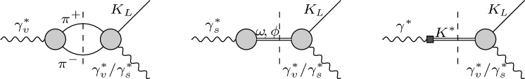
Figure 3: Different contributions to the $K_{L}\to\gamma^{*}\gamma^{*}$ form factor in a dispersive approach. The gray blobs denote the respective hadronic matrix elements, and the black square the strangeness-changing $K^{*}$–$\gamma^{*}$ coupling that is again mediated by vector-meson states.

In the same vain, $M(t,q^{2})=M_{1}(z_{3})/M_{K}^{3}$, the (normalized) multipole for general photon virtuality $q^{2}$, is decomposed as

$$M(t,q^{2})=M_{v}(t,q^{2})+M_{s}(t,q^{2})+M_{K^{*}}(t,q^{2}).$$ (34)

The two-pion cuts then lead to the unsubtracted dispersion relations

$$c_{vv}(q_{1}^{2},q_{2}^{2}) =\frac{e}{12\pi^{2}}\int_{4M_{\pi}^{2}}^{{s_{\text{m}}}}\text{d}x\frac{q_{\pi}^{3}(x)[F_{\pi}^{V}(x)]^{*}M_{v}(x,q_{2}^{2})}{x^{1/2}(x-q_{1}^{2})}$$

$$=\frac{e}{12\pi^{2}}\int_{4M_{\pi}^{2}}^{{s_{\text{m}}}}\text{d}x\frac{q_{\pi}^{3}(x)[F_{\pi}^{V}(x)]^{*}M_{v}(x,q_{1}^{2})}{x^{1/2}(x-q_{2}^{2})},$$

$$c_{vs}(q_{1}^{2},q_{2}^{2}) =\frac{e}{12\pi^{2}}\int_{4M_{\pi}^{2}}^{{s_{\text{m}}}}\text{d}x\frac{q_{\pi}^{3}(x)[F_{\pi}^{V}(x)]^{*}M_{s}(x,q_{2}^{2})}{x^{1/2}(x-q_{1}^{2})},$$

$$c_{sv}(q_{1}^{2},q_{2}^{2}) =\frac{e}{12\pi^{2}}\int_{4M_{\pi}^{2}}^{{s_{\text{m}}}}\text{d}x\frac{q_{\pi}^{3}(x)[F_{\pi}^{V}(x)]^{*}M_{s}(x,q_{1}^{2})}{x^{1/2}(x-q_{2}^{2})},$$ (35)

where $q_{\pi}(x)=\sqrt{x/4-M_{\pi}^{2}}$, $F_{\pi}^{V}$ is the electromagnetic form factor of the pion, and $\sqrt{{s_{\text{m}}}}=2\,\text{GeV}$ denotes a cutoff that separates the low-energy contribution.

2.3.1 Factorization

The simplest solution to the decomposition (34) involves separating the final-state interaction into an Omnès factor Omnès (1958)

$$\Omega_{1}(t)=\exp\bigg{\{}\frac{t}{\pi}\int_{4M_{\pi}^{2}}^{\infty}\text{d}x\frac{\delta_{1}(x)}{x(x-t)}\bigg{\}},$$ (36)

determined by the $P$-wave $\pi\pi$ scattering phase shift $\delta_{1}(t)$, and parameterizing the remainder via polynomials

$$\mathcal{M}(t,q^{2})=\sum_{i=v,s}a_{i}(q^{2})\bigg{[}P_{i}(t)+\epsilon_{K^{*}}\frac{a_{K^{*}}(t)}{a_{K^{*}}(0)}\bigg{]}\Omega_{1}(t),$$ (37)

with $P_{v/s}(t)$ for the isovector/isoscalar contribution, a parameter $\epsilon_{K^{*}}$ for the $K^{*}$, and another function $a_{v/s}(q^{2})$ to describe the dependence on the photon virtuality. In addition,

$$a_{K^{*}}(q^{2})=\frac{1}{\pi}\int_{(M_{K}+M_{\pi})^{2}}^{{s_{\text{m}}}}\text{d}x\frac{\text{Im}\,\text{BW}_{K^{*}}(x)}{x-q^{2}},$$ (38)

where the imaginary part follows a Breit–Wigner description of the $K^{*}$ resonance. Using the ansatz (37), the $c_{vv}$ contribution in Eq. (2.3) can be rewritten as

$$c_{vv}(q_{1}^{2},q_{2}^{2}) =a_{v}(q_{1}^{2})a_{vv}(q_{2}^{2})=a_{v}(q_{2}^{2})a_{vv}(q_{1}^{2}),$$

$$a_{vv}(q^{2}) =\frac{1}{\pi}\int_{4M_{\pi}^{2}}^{{s_{\text{m}}}}\text{d}x\frac{\rho_{vv}(x)}{x-q^{2}},\qquad\rho_{vv}(x)=\frac{eq_{\pi}^{3}(x)[F_{\pi}^{V}(x)]^{*}P_{v}(x)\Omega_{1}(x)}{12\pi\sqrt{x}}.$$ (39)

The first line implies the factorization $a_{vv}(q^{2})=\alpha_{1}a_{v}(q^{2})$. Moreover, Eq. (2.3) remains invariant upon rescaling $a_{v}(q^{2})\to\alpha_{2}a_{v}(q^{2})$, $P_{v}(t)\to P_{v}(t)/\alpha_{2}$, i.e., $a_{vv}(q^{2})=\alpha_{1}\alpha_{2}^{2}a_{v}(q^{2})$. Choosing $\alpha_{2}=1/\sqrt{|\alpha_{1}|}$ therefore shows that

$$c_{vv}(q_{1}^{2},q_{2}^{2})=\pm a_{vv}(q_{1}^{2})a_{vv}(q_{2}^{2}).$$ (40)

It is further instructive to consider the limit of a narrow resonance Hoferichter et al. (2012)

$$a_{vv}(q^{2})\to eF_{\pi}^{2}P_{v}(M_{\rho}^{2})\frac{M_{\rho}^{2}}{M_{\rho}^{2}-q^{2}},$$ (41)

where the KFSR relation Kawarabayashi and Suzuki (1966); Riazuddin and Fayyazuddin (1966) has been used to trade the $\rho\pi\pi$ coupling in favor of the pion decay constant $F_{\pi}$. Up to a normalization, $a_{vv}(q^{2})$ thus reduces to a $\rho$ propagator in the narrow-resonance approximation.

The isoscalar function $a_{s}(q^{2})$ is dominated by $\omega$ and $\phi$ resonances, leading to the ansatz

$$a_{s}(q^{2})=\sum_{V=\omega,\phi}c_{V}\frac{a_{V}(q^{2})}{a_{V}(0)},\qquad a_{V}(q^{2})=\frac{1}{\pi}\int_{s_{\text{th}}}^{{s_{\text{m}}}}\text{d}x\frac{\text{Im}\,\text{BW}_{V}(x)}{x-q^{2}},$$ (42)

with a spectral function determined by a suitable parameterization of the imaginary parts following Hoferichter et al. (2014a, 2018a, 2018b). In the limit of a narrow resonance, this form becomes identical to Eq. (41) upon identifying $c_{\rho}=eF_{\pi}^{2}P_{v}(M_{\rho}^{2})$. For the mixed isovector–isoscalar contribution we have

$$c_{vs}(q_{1}^{2},q_{2}^{2}) =a_{s}(q_{2}^{2})a_{vs}(q_{1}^{2}),$$

$$a_{vs}(q^{2}) =\frac{1}{\pi}\int_{4M_{\pi}^{2}}^{{s_{\text{m}}}}\text{d}x\frac{\rho_{vs}(x)}{x-q^{2}},\qquad\rho_{vs}(x)=\frac{eq_{\pi}^{3}(x)[F_{\pi}^{V}(x)]^{*}P_{s}(x)\Omega_{1}(x)}{12\pi\sqrt{x}},$$ (43)

where the difference to $a_{vv}(q^{2})$ solely originates from the polynomial $P_{v/s}(t)$. Finally, for the isoscalar–isoscalar contribution we set

$$c_{ss}(q_{1}^{2},q_{2}^{2})=\sum_{V,V^{\prime}=\omega,\phi}c_{VV^{\prime}}\frac{a_{V}(q_{1}^{2})}{a_{V}(0)}\frac{a_{V^{\prime}}(q_{2}^{2})}{a_{V^{\prime}}(0)},$$ (44)

in analogy to Eq. (42). For the actual application, we further need to determine the overall sign and the relative size of the various isospin components, a point to which we will return in Sec. 2.4.

The remaining parts enter in the context of the $K^{*}$ contribution, the third diagram in Fig. 3. To evaluate this diagram, we analyze the double discontinuity arising from the two-pion and $\pi K\simeq K^{*}$ intermediate states, in analogy to $2\pi$ and $3\pi$ singularities in the context of $\rho$–$\omega$ mixing in Ref. Hoferichter et al. (2016). We obtain the result

$$c_{vK^{*}}(q_{1}^{2},q_{2}^{2}) =\pm a_{vv}(q_{1}^{2})\epsilon_{K^{*}}\frac{a_{K^{*}}(q_{2}^{2})}{a_{K^{*}}(0)}2a_{\rho}(0)$$

$$\times\text{Re}\,\bigg{[}\bigg{(}1+\frac{\beta_{K^{*}}}{3}\bigg{)}-\frac{a_{\rho}(q_{2}^{2})}{a_{\rho}(0)}-\frac{\beta_{K^{*}}}{3}\bigg{(}\frac{1}{3}\frac{a_{\omega}(q_{2}^{2})}{a_{\omega}(0)}+\frac{2}{3}\frac{a_{\phi}(q_{2}^{2})}{a_{\phi}(0)}\bigg{)}\bigg{]},$$ (45)

where the overall sign is related to the one in $c_{vv}(q_{1}^{2},q_{2}^{2})$ and the same expression holds for $c_{sK^{*}}(q_{1}^{2},q_{2}^{2})$ with $a_{vv}(q_{1}^{2})\to a_{s}(q_{1}^{2})$. The contribution from the $\rho$ can be derived from the double discontinuity, leading to

$$a_{\rho}(q^{2})=\frac{1}{\pi}\int_{4M_{\pi}^{2}}^{{s_{\text{m}}}}\text{d}x\frac{\rho_{\rho}(x)}{x-q^{2}},\qquad\rho_{\rho}(x)=\frac{eq_{\pi}^{3}(x)[F_{\pi}^{V}(x)]^{*}\Omega_{1}(x)}{12\pi\sqrt{x}},$$ (46)

which coincides with $a_{vv}(q^{2})$, $a_{vs}(q^{2})$ in the limit $P_{v/s}(t)=1$. The coefficients of the $\omega$ and $\phi$ contributions are parameterized in analogy to the BMS ansatz (18), with the propagators replaced by a dispersively improved Breit–Wigner prescription as defined in Eq. (42). The remaining free parameters are $\epsilon_{K^{*}}$ and $\beta_{K^{*}}$, where the latter is necessary to accommodate the slope parameter (19).

Factorization-breaking contributions to $M_{v/s}(t,q^{2})$ are generated when including left-hand cuts (LHCs), which are expanded in a polynomial in Eq. (37). Neglecting isospin-breaking contributions, the leading LHCs to $K_{L}\to\pi^{+}\pi^{-}\gamma^{*}$ arise from a pion pole (for $M_{v}(t,q^{2})$) and two-pion intermediate states (for $M_{s}(t,q^{2})$). Since the former involves a $K_{L}\to\pi\pi$ vertex, this contribution will be $CP$ violating. The two-pion LHC in $M_{s}(t,q^{2})$ conserves $CP$, but involves an anomalous $\gamma 3\pi$ vertex (and only appears in the isoscalar amplitude). Accordingly, the role of LHCs beyond their polynomial approximation should be negligible, especially in the limited kinematic domain accessible in the kaon decay.

2.3.2 Fits to $\boldsymbol{K_{L}\to\pi^{+}\pi^{-}\gamma}$

As anticipated in Sec. 2.2, experiments have observed evidence for an $E_{\gamma}^{*}$-dependent form-factor modification in contrast to a pure-$M_{1}$ DE amplitude Ramberg et al. (1993); Alavi-Harati et al. (2001c); Abouzaid et al. (2006). This enables us to determine the polynomial in Eq. (37). Accordingly, we perform a linear-polynomial fit to the spectrum data from Refs. Alavi-Harati et al. (2001c) by

$$P_{v/s}(t)=N_{v/s}(1+\alpha_{v/s}t).$$ (47)

In the singly-virtual decay, it is not possible to separate all isospin components, instead, the spectrum is sensitive to the parameter combinations

$$N_{\pi\pi} =a_{vv}(0)N_{v}+a_{s}(0)N_{s},\qquad b_{\pi\pi}=a_{vv}(0)N_{v}\alpha_{v}+a_{s}(0)N_{s}\alpha_{s},$$

$$\eta_{K^{*}} =(a_{vv}(0)+a_{s}(0))\epsilon_{K^{*}}.$$ (48)

$N_{\pi\pi}[\,\text{GeV}^{-3}]$	$\bar{b}_{\pi\pi}[\,\text{GeV}^{-2}]$	$\bar{\eta}_{K^{*}}$	$\chi^{2}/\text{dof}$	$p$-value
$3.47(27)\times 10^{-8}$	$10.0(1.9)$	$0.96(10)$	$34.1/27=1.26$	$16.3\%$

Table 1: Fit to the $K_{L}\to\pi^{+}\pi^{-}\gamma$ spectrum from Ref. Alavi-Harati et al. (2001c), see main texts for more details.

In particular, it is useful to rewrite the amplitude as

$$N_{\pi\pi}\bigg{[}1+\bar{b}_{\pi\pi}t+\bar{\eta}_{K^{*}}\frac{a_{K^{*}}(t)}{a_{K^{*}}(0)}\bigg{]},$$ (49)

with

$$b_{\pi\pi}=N_{\pi\pi}\bar{b}_{\pi\pi},\qquad\eta_{K^{*}}=N_{\pi\pi}\bar{\eta}_{K^{*}},$$ (50)

to isolate normalization and $t$ dependence in the fit. Ideally, one should then perform a combined analysis of all data for the spectra of the leptonic decays $K_{L}\to\ell^{+}\ell^{-}\gamma$ and the hadronic channel $K_{L}\to\pi^{+}\pi^{-}\gamma$, in order to disentangle the linear term in Eq. (49) from the $K^{*}$ contribution. Unfortunately, the original data for these spectra are rarely available: the best measurements of $K_{L}\to e^{+}e^{-}\gamma$ Abouzaid et al. (2007) and $K_{L}\to\mu^{+}\mu^{-}\gamma$ Alavi-Harati et al. (2001a) are only provided in terms of fits using the two models introduced in Sec. 2.1, but the original data for the spectrum are not included in the publications. Similarly, we could only obtain the $K_{L}\to\pi^{+}\pi^{-}\gamma$ data from Ref. Alavi-Harati et al. (2001c) by digitizing Fig. 4 therein (we checked that a fit to the digitized data reproduces the fit parameters given in the paper), while the spectra from Refs. Ramberg et al. (1993); Abouzaid et al. (2006) are not accessible at all.

Given the high degree of correlation between the linear polynomial and the $K^{*}$ piece, the constraints from the dilepton data are critical, in such a way that we do need to rely on the value of $\eta_{K^{*}}$ inferred from the global average of $\alpha_{K^{*}}$ Workman et al. (2022). Accordingly, we will also use the slope determination via the BMS parameterization (19), to ensure a consistent set of input quantities. The resulting residual model dependence could be avoided if the spectral data from Refs. Abouzaid et al. (2007); Alavi-Harati et al. (2001a); Ramberg et al. (1993); Abouzaid et al. (2006) were available. With $\eta_{K^{*}}$ constrained to its BMS value, we then fit the remaining parameters $N_{\pi\pi}$ and $\bar{b}_{\pi\pi}$ to the spectrum from Ref. Alavi-Harati et al. (2001c), first, with normalization in arbitrary units. In a final step, $N_{\pi\pi}$ is rescaled to reproduce the total DE decay rate Workman et al. (2022), for which our fit produces an uncertainty estimate consistent with Ref. Alavi-Harati et al. (2001c) after taking into account the correlations between the fit parameters. The fit results are shown in Table 1 and Fig. 4, and will serve as basis for the error estimate of the dispersive form factor in Sec. 5.

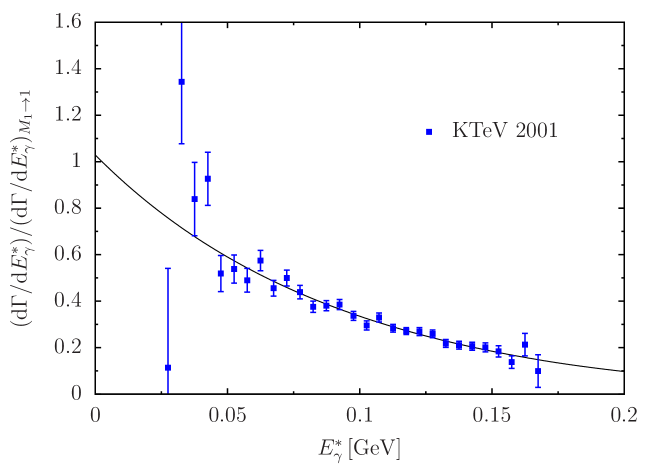
Figure 4: Fit to the $K_{L}\to\pi^{+}\pi^{-}\gamma$ differential decay rate, using the data from Ref. Alavi-Harati et al. (2001c). Vertical scale in arbitrary units.

2.4 Vector meson dominance

The $K_{L}\to\pi^{+}\pi^{-}\gamma$ channel only determines the sum of the isovector and isoscalar parameters in the form of Eq. (2.3.2) as they enter in the singly-virtual form factor, but not the relative weights between the different isospin contributions. In such a situation, the vector-meson-dominance (VMD) picture often provides useful information to constrain the relative strength of different isospin components in the doubly-virtual form factor as well, see, e.g., Refs. Klingl et al. (1996); Gan et al. (2022); Zanke et al. (2021).

The $SU(3)$ pseudoscalar matrix $|\phi\rangle$ transforms under $CP$ as $CP|\phi\rangle=-|\phi\rangle^{T}$. The phase in front is fixed by the $CP$ quantum numbers of the neutral states, e.g., from $CP|\pi^{0}\rangle=-|\pi^{0}\rangle$. Thereafter, the $K_{L}$ state is defined as $(|K^{0}\rangle+|\bar{K^{0}}\rangle)/\sqrt{2}$, in line with the prescription applied in Ref. Ecker and Pich (1991). After identifying the phase convention in this way, we can write down the simplest trace that correctly projects out the $K_{L}$ state,

$$\text{Tr}\big{(}\{\lambda_{6},|\phi\rangle\}|V\rangle|V\rangle\big{)},$$ (51)

where $|V\rangle$ is the vector-meson nonet matrix and we assume ideal mixing for $\omega$ and $\phi$. Adding the relative factors from the $V\gamma$ couplings Klingl et al. (1996); Hoferichter et al. (2017); Zanke et al. (2021), the relative weights between the different contributions to the form-factor normalization read

$$c_{vv}(0,0):c_{vs}(0,0):c_{ss}(0,0)=1:-\frac{1}{3}:\frac{5}{9}.$$ (52)

The same calculation also predicts the relative size of $\omega$ and $\phi$ contributions to $a_{s}(q^{2})$ and $a_{ss}(q_{1}^{2},q_{2}^{2})$, in particular

$$c_{\phi}=0,\qquad c_{\phi\omega}=c_{\omega\phi}=0,\qquad c_{\phi\phi}=4c_{\omega\omega}.$$ (53)

Similarly, the trace

$$\text{Tr}\big{(}\{\lambda_{6},|V\rangle\}|V\rangle\big{)},$$ (54)

in combination with the $V\gamma$ couplings, predicts the relative size of the $K^{*}$–$\gamma$ transitions

$$c_{K^{*}\to\rho\to\gamma}:c_{K^{*}\to\omega\to\gamma}:c_{K^{*}\to\phi\to\gamma}=1:-\frac{1}{3}:\frac{2}{3}.$$ (55)

These ratios differ from the ones assumed in the BMS model (18), $1:1/9:2/9$, which are obtained when removing the singlet from $|V\rangle$ in Eq. (54), as done in Ref. Sarraga and Munczek (1971). The two variants give an identical decomposition into isoscalar and isovector contributions, but the relative size of $\omega$ and $\phi$ differs. Although the resulting change in the $K^{*}$ parameterization (2.3.1) scales with $M_{\phi}-M_{\omega}$, we observe that the effect is numerically significant. Accordingly, since we need to rely on $\epsilon_{K^{*}}$ from the BMS fits, we employ the same decomposition of $\omega$ and $\phi$, leading to the form anticipated in Eq. (2.3.1). Finally, while the normalizations $c_{vK^{*}}(0,0)=c_{sK^{*}}(0,0)$ vanish by construction, we can consider the ratio

$$\frac{c_{vK^{*}}(q_{1}^{2},q_{2}^{2})}{c_{sK^{*}}(q_{1}^{2},q_{2}^{2})}=\frac{a_{vv}(q_{1}^{2})}{a_{s}(q_{1}^{2})},$$ (56)

which is constrained in the dispersive approach in terms of $a_{vv}(q^{2})$ and $a_{s}(q^{2})$. Here, VMD predicts the same relative weights of $\rho$, $\omega$, and $\phi$ as in Eq. (55), which does not agree with $c_{\phi}=0$ in $a_{s}(q^{2})$, i.e., in a similar way as in the comparison to the BMS parameterization we observe an ambiguity in the separation of $\omega$ and $\phi$ contributions. The relative normalization

$$\frac{c_{vK^{*}}(0,q_{2}^{2})}{c_{sK^{*}}(0,q_{2}^{2})}=\frac{a_{vv}(0)}{a_{s}(0)}=3$$ (57)

is again not affected, and this constraint proves very useful for disentangling the different normalizations, see Sec. 4. Beyond, we set

$$c_{\phi}=2c_{\omega},$$ (58)

for consistency with Eq. (2.3.1) and the BMS input for the $K^{*}$ piece, while for the non-$K^{*}$ contributions we keep the (internally consistent) set of conditions (52) and (53).

Ultimately, the impact of these VMD assumptions on the final uncertainty proves relatively minor, for the following reasons: the singly-virtual form factor is probed directly in terms of $K_{L}\to\ell^{+}\ell^{-}\gamma$ and $K_{L}\to\pi^{+}\pi^{-}\gamma$, so that VMD arguments only enter in the doubly-virtual direction. Second, the ambiguities related to $\omega$ and $\phi$ only affect the internal decomposition of the isoscalar contribution, and, e.g., the three variants $c_{\phi}=\pm 2c_{\omega}$, $c_{\phi}=0$ for the $K^{*}$ affect $\text{Re}\,\mathcal{A}_{\mu}(M_{K}^{2})$ at a level below $0.1$. In general, we find that the result for the reduced amplitude $\text{Re}\,\mathcal{A}_{\ell}(M_{K}^{2})$ is rather robust against variation of the relative VMD weights, see Sec. 5, once the constraints from the form factor normalization (12) and slope (19) are imposed. As discussed in Sec. 4, only one of the relative normalizations (52) needs to be provided to determine all parameters, so that choosing either one of them serves as a way to assess the impact of the VMD assumptions, and the corresponding variation will be included in the uncertainty estimate for the dispersive part of the form factor quoted in Sec. 5.

3 Matching to asymptotic constraints

Figure 5: Partonic diagrams for $K_{L}\to\gamma^{*}\gamma^{*}$.

The asymptotic form of $c(q_{1}^{2},q_{2}^{2})$ was constrained in Ref. Isidori and Unterdorfer (2004) using arguments from a partonic calculation, which we will incorporate here in our dispersive representation. The key result reads

$$c^{\text{asym}}(q_{1}^{2},q_{2}^{2})=\frac{16\alpha G_{F}V_{us}^{*}V_{ud}F_{K}}{9\pi\sqrt{2}}\big{[}C_{2}(\mu)+3C_{1}(\mu)\big{]}\bigg{[}I(q_{1}^{2},q_{2}^{2})+T(q_{1}^{2})+T(q_{2}^{2})\bigg{]},$$ (59)

with tree-level Wilson coefficients normalized as $C_{2}(M_{W})=1$, $C_{1}(M_{W})=0$. The loop functions originate from diagrams with $c$- and $u$-quark loops as depicted in Fig. 5, where either both photons couple in the loop, $I(q_{1}^{2},q_{2}^{2})$, or just one, $T(q_{i}^{2})$, and result from the difference of the two flavors. However, we note that Eq. (59) as in Ref. Isidori and Unterdorfer (2004) is valid for deeply-virtual kinematics and up to power-suppressed terms of $\mathcal{O}(\xi)$, $\xi=m_{u}^{2}/m_{c}^{2}$. In order to establish a matching between the low-energy dispersive contributions and the asymptotic constraints, we start from the full expressions including the dependence on $m_{u}$, and separate the low- and high-energy contributions by introducing a cutoff in a dispersive representation of the respective loop integrals, see App. B for details.

3.1 Two-point function

The starting point for $T(q^{2})$ is given by the usual vacuum polarization from a quark loop, i.e.,

$$T(q^{2}) =T_{c}(q^{2})-T_{u}(q^{2})=2\int_{0}^{1}\text{d}x\,x(1-x)\log\Big{[}1-x(1-x)\frac{q^{2}}{m_{c}^{2}}\Big{]}-(c\leftrightarrow u)$$

$$=2\int_{0}^{1}\text{d}x\,x(1-x)\log\frac{1-x(1-x)r}{\xi-x(1-x)r}+\frac{1}{3}\log\xi,\qquad r=\frac{q^{2}}{m_{c}^{2}}.$$ (60)

It is clear that $T(r)$ does not contribute to the form factor normalization, a property that should be preserved when removing the low-energy contributions. Moreover, for $q^{2}\to\infty$ the difference of $c$- and $u$-quark integrals decreases as $1/q^{2}$, which should also be reflected by the final representation.

The definition of $T(q^{2})$ in Ref. Isidori and Unterdorfer (2004) follows when dropping the $\log\xi$ term and the dependence on $\xi$ in the integral (3.1), i.e.,

$$T(r)\big{|}_{\text{\cite[cite]{\@@bibref{Authors Phrase1YearPhrase2}{Isidori:2003ts}{\@@citephrase{(}}{\@@citephrase{)}}}}}=2\int_{0}^{1}\text{d}x\,x(1-x)\log\frac{1-x(1-x)r}{-x(1-x)r}.$$ (61)

This loop function has a good asymptotic behavior for $r\to\infty$

$$T(-r_{1})+T(-r_{2})=\frac{2}{r_{1}}+\frac{2}{r_{2}}=\frac{8}{r_{1}+r_{2}}\bigg{[}1+\mathcal{O}\bigg{(}\frac{(r_{1}-r_{2})^{2}}{(r_{1}+r_{2})^{2}}\bigg{)}\bigg{]},$$ (62)

but displays a sensitivity to infrared scales. In particular, $T(r)$ is now divergent for $r\to 0$, as can be made explicit by rewriting Eq. (61) as

$$T(r)\big{|}_{\text{\cite[cite]{\@@bibref{Authors Phrase1YearPhrase2}{Isidori:2003ts}{\@@citephrase{(}}{\@@citephrase{)}}}}}=2\int_{0}^{1}\text{d}x\,x(1-x)\log\big{[}1-x(1-x)r\big{]}+\frac{5}{9}-\frac{1}{3}\log(-r).$$ (63)

For the asymptotic matching, we thus need to impose integration cutoffs in the dispersive representation for $T(q^{2})$

$$T^{\text{asym}}(q^{2})=T_{c}^{\text{asym}}(q^{2})-T_{u}^{\text{asym}}(q^{2})=-\frac{q^{2}}{3}\bigg{[}\int_{s_{c}}^{\infty}\text{d}s\frac{\sigma_{c}(s)(s+2m_{c}^{2})}{s^{2}(s-q^{2})}-\int_{s_{u}}^{\infty}\frac{\text{d}s}{s(s-q^{2})}\bigg{]},$$ (64)

where $\sigma_{q}(s)=\sqrt{1-4m_{q}^{2}/s}$, see Eq. (B.1). Here, the integration cutoffs $s_{u}$ and $s_{c}$ are related to ensure the correct asymptotic behavior, e.g., for the canonical choice $s_{c}=4m_{c}^{2}$ one has $s_{u}=\mathrm{e}^{5/3}m_{c}^{2}\simeq 5.29m_{c}^{2}$.

3.2 Three-point function

As detailed in App. B, the full loop function

$$I(q_{1}^{2},q_{2}^{2})=I_{c}(q_{1}^{2},q_{2}^{2})-(c\leftrightarrow u)$$ (65)

can be reconstructed from Refs. Simma and Wyler (1990); Herrlich and Kalinowski (1992). The resulting expression is well-defined for all virtualities, thus correctly reproduces the partonic contributions to the real-photon kinematics obtained in Refs. Gaillard and Lee (1974); Ma and Pramudita (1981), i.e., it simplifies to

$$I_{c}(0,0)=-1-\frac{2}{r_{3}}\int_{0}^{1}\text{d}x\frac{\log\big{[}1-r_{3}x(1-x)\big{]}}{x},$$ (66)

where $r_{3}=M_{K}^{2}/m_{c}^{2}$. We also reproduce the result of Ref. Isidori and Unterdorfer (2004), by taking $r_{3}=0$ and combining the $u$- and $c$-quark contributions,

$$I(r_{1},r_{2})\big{|}_{\text{\cite[cite]{\@@bibref{Authors Phrase1YearPhrase2}{Isidori:2003ts}{\@@citephrase{(}}{\@@citephrase{)}}}}} =\frac{1}{6}+\int_{0}^{1}dx\int_{0}^{1-x}dy\bigg{\{}\frac{2-x-y+(r_{1}x+r_{2}y)(1-x-y)^{2}}{1-(r_{1}x+r_{2}y)(1-x-y)}$$

$$-(2-3x-3y)\log\frac{1-(r_{1}x+r_{2}y)(1-x-y)}{-(r_{1}x+r_{2}y)(1-x-y)}\bigg{\}}+\mathcal{O}(\xi\log\xi).$$ (67)

Although the limit $\xi\to 0$ is finite, the final expression in Eq. (3.2) is not well-defined for all virtualities, and we again need to isolate the low- and high-energy contributions by imposing a cutoff in the dispersive representation.

As a first step, we analyzed the discontinuities of $I_{c}(q_{1}^{2},q_{2}^{2})$, which shows that even for general $r_{3}$ the expression reduces to a simple scalar loop integral

$$I_{q}(q_{1}^{2},q_{2}^{2})=-2C_{0}(r_{1},r_{2},r_{3})-1,$$ (68)

with $C_{0}$ as defined in Eq. (125). Moreover, the analysis in App. B shows that upon introducing a cutoff $s_{u}$ in the dispersion relation, no infrared singularities occur and the limit $m_{u}\to 0$ can be taken, in such a way that

$$I_{u}(q_{1}^{2},q_{2}^{2})\to-1,$$ (69)

i.e., no non-trivial contributions remain from the $u$-quark loop. For the $c$-quark loop, setting $M_{K}=0$ permits a very simple double-spectral representation of the form

$$I_{c}(q_{1}^{2},q_{2}^{2}) =-1+\frac{m_{c}^{2}}{\pi^{2}}\int_{s_{c}}^{\infty}\text{d}x\int_{s_{c}}^{\infty}\text{d}y\frac{2\pi^{2}\delta(x-y)\log\frac{1+\sigma_{c}(x)}{1-\sigma_{c}(x)}}{(x-q_{1}^{2})(y-q_{2}^{2})}$$

$$=-1+\frac{m_{c}^{2}}{\pi}\int_{s_{c}}^{\infty}\text{d}x\frac{2\pi\log\frac{1+\sigma_{c}(x)}{1-\sigma_{c}(x)}}{(x-q_{1}^{2})(x-q_{2}^{2})}.$$ (70)

A generalization of the de-facto single-variable dispersion relation in the second line to the case $M_{K}>0$ is given in Eq. (130), while a full double-spectral representation requires a contour deformation according to Eq. (138). We observed that the numerical difference between the $M_{K}=0$ simplified form and the full representation (138) is negligible for the current application.

4 Final representation

4.1 Decomposition of $\boldsymbol{K_{L}\to\gamma^{*}\gamma^{*}}$ form factor

To derive the final representation we first need to establish the sign convention for the $K_{L}\to\gamma^{*}\gamma^{*}$ form factor $c(q_{1}^{2},q_{2}^{2})$. A detailed discussion of the sign of the SD contribution relative to the LD part is provided in Ref. Isidori and Unterdorfer (2004), under the assumption that the dominant contribution to $\mathcal{A}^{\mu\nu}[K_{L}\to\gamma\gamma]$ arises from the $\pi^{0}$ pole

$$c(0,0)\big{|}_{\pi^{0}}=\frac{2G_{8}F_{\pi}\alpha}{\pi}\frac{M_{K}^{2}}{M_{K}^{2}-M_{\pi}^{2}},\qquad\big{|}c(0,0)\big{|}_{\pi^{0}}\simeq 4.2\times 10^{-9}\,\text{GeV}^{-1},$$ (71)

indeed close to the experimental value $|c(0,0)|=3.389(14)\times 10^{-9}\,\text{GeV}^{-1}$. Accordingly, it seems safe to assume that the signs of $\mathcal{A}[K_{L}\to\gamma\gamma]$ and $\mathcal{A}[K_{L}\to\pi^{0}\to\gamma\gamma]$ coincide. The sign of $G_{8}$ cannot be extracted from experiment, but it can be determined by considering hadronic matrix elements of four-quark operators in the $\Delta S=1$ Lagrangian, $\langle\pi^{0}|\mathcal{H}_{W}|K_{L}\rangle$, in a factorization assumption, which leads to $G_{8}<0$ Pich and de Rafael (1996); Buchalla et al. (2003). This conclusion agrees with large-$N_{c}$ considerations Gómez Dumm and Pich (1998); Knecht et al. (1999), and we will therefore adopt

$$c(0,0)=-3.389(14)\times 10^{-9}\,\text{GeV}^{-1}$$ (72)

as boundary condition. The final representation is then decomposed as

$$c(q_{1}^{2},q_{2}^{2})=c^{\text{disp}}(q_{1}^{2},q_{2}^{2})+c^{\text{asym}}(q_{1}^{2},q_{2}^{2}),$$ (73)

where the asymptotic contribution follows as given in Sec. 3

$$c^{\text{asym}}(q_{1}^{2},q_{2}^{2}) =\frac{16\alpha G_{F}V_{us}^{*}V_{ud}F_{K}}{9\pi\sqrt{2}}\big{[}C_{2}(\mu)+3C_{1}(\mu)\big{]}\bigg{\{}\frac{m_{c}^{2}}{\pi}\int_{s_{c}}^{\infty}\text{d}x\frac{2\pi\log\frac{1+\sigma_{c}(x)}{1-\sigma_{c}(x)}}{(x-q_{1}^{2})(x-q_{2}^{2})}$$

$$-\sum_{i=1,2}\frac{q_{i}^{2}}{3}\bigg{[}\int_{s_{c}}^{\infty}\text{d}s\frac{\sigma_{c}(s)(s+2m_{c}^{2})}{s^{2}(s-q_{i}^{2})}-\int_{s_{u}}^{\infty}\frac{\text{d}s}{s(s-q_{i}^{2})}\bigg{]}\bigg{\}},$$ (74)

with $s_{c}=4m_{c}^{2}$, $s_{u}=\mathrm{e}^{5/3}m_{c}^{2}$, and Wilson coefficients $C_{i}(\mu)$ including the QCD renormalization group (RG) running from Ref. Buchalla et al. (1996) to resum the large logarithms $(\alpha_{s}\log M_{W}/\mu)^{n}$ and $\alpha_{s}(\alpha_{s}\log M_{W}/\mu)^{n}$ to all orders in $\alpha_{s}$. The scale is set to $\mu^{2}=|q_{1}^{2}+q_{2}^{2}|/2$, and the $C_{i}(\mu)$ are kept constant below $\mu_{\text{cut}}=2\,\text{GeV}$. Since the RG corrections to the linear combination $C_{2}+3C_{1}$ happen to be large, canceling a significant part of the tree-level result, it is worthwhile to also consider the next-to-leading-order RG corrections from Ref. Buchalla et al. (1996) to obtain a more realistic estimate of the perturbative uncertainty, despite the dependence on the scheme for $\gamma_{5}$. We choose the result in the ’t Hooft–Veltman scheme ’t Hooft and Veltman (1972) as our central value, and the variation to the leading-order RG and naive dimensional regularization as an estimate of the uncertainty. $c^{\text{asym}}(0,0)$ then contributes only $2.1\%$ to the form factor normalization, while the correction to the slope is negligible.

In our final representation, the dispersive part is decomposed according to

$$c^{\text{disp}}(q_{1}^{2},q_{2}^{2}) =c_{vv}(q_{1}^{2},q_{2}^{2})+c_{vs}(q_{1}^{2},q_{2}^{2})+c_{sv}(q_{1}^{2},q_{2}^{2})+c_{ss}(q_{1}^{2},q_{2}^{2})$$

$$+c_{vK^{*}}(q_{1}^{2},q_{2}^{2})+c_{K^{*}v}(q_{1}^{2},q_{2}^{2})+c_{sK^{*}}(q_{1}^{2},q_{2}^{2})+c_{K^{*}s}(q_{1}^{2},q_{2}^{2}),$$ (75)

with

$$c_{vv}(q_{1}^{2},q_{2}^{2}) =-a_{vv}(q_{1}^{2})a_{vv}(q_{2}^{2}),$$

$$c_{vs}(q_{1}^{2},q_{2}^{2}) =-a_{vs}(q_{1}^{2})a_{s}(q_{2}^{2}),$$

$$c_{ss}(q_{1}^{2},q_{2}^{2}) =-a_{ss}(q_{1}^{2},q_{2}^{2}),$$

$$c_{vK^{*}}(q_{1}^{2},q_{2}^{2}) =-a_{vv}(q_{1}^{2})\epsilon_{K^{*}}\frac{a_{K^{*}}(q_{2}^{2})}{a_{K^{*}}(0)}2a_{\rho}(0)$$

$$\times\text{Re}\,\bigg{[}\bigg{(}1+\frac{\beta_{K^{*}}}{3}\bigg{)}-\frac{a_{\rho}(q_{2}^{2})}{a_{\rho}(0)}-\frac{\beta_{K^{*}}}{3}\bigg{(}\frac{1}{3}\frac{a_{\omega}(q_{2}^{2})}{a_{\omega}(0)}+\frac{2}{3}\frac{a_{\phi}(q_{2}^{2})}{a_{\phi}(0)}\bigg{)}\bigg{]},$$

$$c_{sK^{*}}(q_{1}^{2},q_{2}^{2}) =-a_{s}^{K^{*}}(q_{1}^{2})\epsilon_{K^{*}}\frac{a_{K^{*}}(q_{2}^{2})}{a_{K^{*}}(0)}2a_{\rho}(0)$$

$$\times\text{Re}\,\bigg{[}\bigg{(}1+\frac{\beta_{K^{*}}}{3}\bigg{)}-\frac{a_{\rho}(q_{2}^{2})}{a_{\rho}(0)}-\frac{\beta_{K^{*}}}{3}\bigg{(}\frac{1}{3}\frac{a_{\omega}(q_{2}^{2})}{a_{\omega}(0)}+\frac{2}{3}\frac{a_{\phi}(q_{2}^{2})}{a_{\phi}(0)}\bigg{)}\bigg{]},$$ (76)

$c_{vs}(q_{1}^{2},q_{2}^{2})=c_{sv}(q_{2}^{2},q_{1}^{2})$, $c_{vK^{*}}(q_{1}^{2},q_{2}^{2})=c_{K^{*}v}(q_{2}^{2},q_{1}^{2})$, $c_{sK^{*}}(q_{1}^{2},q_{2}^{2})=c_{K^{*}s}(q_{2}^{2},q_{1}^{2})$, and

$$a_{vv}(q^{2}) =\frac{eN_{v}}{12\pi^{2}}\int_{4M_{\pi}^{2}}^{{s_{\text{m}}}}\text{d}x\frac{q_{\pi}^{3}(x)[F_{\pi}^{V}(x)]^{*}\Omega_{1}(x)(1+\alpha_{v}x)}{x^{1/2}(x-q^{2})},$$

$$a_{vs}(q^{2}) =\frac{eN_{s}}{12\pi^{2}}\int_{4M_{\pi}^{2}}^{{s_{\text{m}}}}\text{d}x\frac{q_{\pi}^{3}(x)[F_{\pi}^{V}(x)]^{*}\Omega_{1}(x)(1+\alpha_{s}x)}{x^{1/2}(x-q^{2})},$$

$$a_{s}(q^{2}) =a_{s}(0)\frac{a_{\omega}(q^{2})}{a_{\omega}(0)},\qquad a_{s}^{K^{*}}(q^{2})=\frac{a_{s}(0)}{3}\bigg{[}2\frac{a_{\phi}(q^{2})}{a_{\phi}(0)}+\frac{a_{\omega}(q^{2})}{a_{\omega}(0)}\bigg{]},$$

$$a_{ss}(q_{1}^{2},q_{2}^{2}) =\frac{a_{ss}(0)}{5}\bigg{[}4\frac{a_{\phi}(q_{1}^{2})}{a_{\phi}(0)}\frac{a_{\phi}(q_{2}^{2})}{a_{\phi}(0)}+\frac{a_{\omega}(q_{1}^{2})}{a_{\omega}(0)}\frac{a_{\omega}(q_{2}^{2})}{a_{\omega}(0)}\bigg{]},$$ (77)

where

$$a_{\rho}(q^{2}) =\frac{e}{12\pi^{2}}\int_{4M_{\pi}^{2}}^{{s_{\text{m}}}}\text{d}x\frac{q_{\pi}^{3}(x)[F_{\pi}^{V}(x)]^{*}\Omega_{1}(x)}{x^{1/2}(x-q^{2})}=\frac{1}{\pi}\int_{4M_{\pi}^{2}}^{{s_{\text{m}}}}\text{d}x\frac{\rho_{\rho}(x)}{x-q^{2}},$$

$$a_{\omega/\phi/K^{*}}(q^{2}) =\frac{1}{\pi}\int_{s_{\text{th}}}^{{s_{\text{m}}}}\text{d}x\frac{\text{Im}\,\text{BW}_{\omega/\phi/K^{*}}(x)}{x-q^{2}}.$$ (78)

4.2 Determination of parameters

The free parameters ($N_{s/v}$, $\alpha_{s/v}$, $a_{s}(0)$, $a_{ss}(0)$, $\epsilon_{K^{*}}$, $\beta_{K^{*}}$) are determined from the following constraints:

1. the fit to $K_{L}\to\pi^{+}\pi^{-}\gamma$, together with the global average for $\alpha_{K^{*}}$ from Ref. Workman et al. (2022), determines the three quantities $N_{\pi\pi}$, $b_{\pi\pi}$, and $\eta_{K^{*}}$ as defined in Eq. (2.3.2),

2. the total normalization $c^{\text{disp}}(0,0)+c^{\text{asym}}(0,0)$ reproduces Eq. (72),

3. VMD predicts the relative normalizations of $c_{vv}(0,0)$, $c_{vs}(0,0)$, and $c_{ss}(0,0)$ as in Eq. (52) and the ratio $a_{vv}(0)/a_{s}(0)$ as in Eq. (57),

4. the total slope reproduces Eq. (19).

To determine the number of independent parameters, we first observe that

$$a_{\rho}(0)N_{\pi\pi}+\bar{a}_{\rho}b_{\pi\pi}=\big{[}a_{vv}(0)\big{]}^{2}+a_{s}(0)a_{vs}(0),\qquad\bar{a}_{\rho}=\frac{1}{\pi}\int_{4M_{\pi}^{2}}^{{s_{\text{m}}}}\text{d}x\,\rho_{\rho}(x).$$ (79)

Accordingly, the quantities in Eq. (2.3.2) (with results collected in Table 1), the total normalization (72), and one of the relative VMD weights given in Eq. (52) allow one to separate the individual terms in

$$c^{\text{disp}}(0,0)=-\big{[}a_{vv}(0)\big{]}^{2}-2a_{s}(0)a_{vs}(0)-a_{ss}(0,0),$$ (80)

and choosing either one of the three relative VMD ratios serves as an estimate of the theoretical uncertainty. The product $a_{s}(0)a_{vs}(0)$ is resolved by employing Eq. (57).

Next, we observe that

$$a_{vv}(q^{2})a_{vv}(0)+a_{vs}(q^{2})a_{s}(0)=a_{\rho}(q^{2})N_{\pi\pi}+\big{(}a_{\rho}(q^{2})q^{2}+\bar{a}_{\rho}\big{)}b_{\pi\pi},$$ (81)

which, together with the normalizations $a_{vv}(0)$, $a_{vs}(0)$, $a_{s}(0)$, and $a_{ss}(0,0)$, is sufficient to determine the singly-virtual dependence in the first line of Eq. (4.1), since $a_{s}(q^{2})$ and $a_{ss}(q_{1}^{2},q_{2}^{2})$ do not involve further free parameters. In contrast, $a_{vv}(q^{2})$ and $a_{vs}(q^{2})$ are more difficult to disentangle. The definitions of $N_{\pi\pi}$, $b_{\pi\pi}$ in Eq. (2.3.2) and of $a_{vv}(0)$, $a_{vs}(0)$ in Eq. (4.1) imply the singular system of equations

$$\begin{pmatrix}a_{vv}(0)&a_{s}(0)&0&0\\ 0&0&a_{vv}(0)&a_{s}(0)\\ a_{\rho}(0)&0&\bar{a}_{\rho}&0\\ 0&a_{\rho}(0)&0&\bar{a}_{\rho}\end{pmatrix}\begin{pmatrix}N_{v}\\ N_{s}\\ N_{v}\alpha_{v}\\ N_{s}\alpha_{s}\end{pmatrix}=\begin{pmatrix}N_{\pi\pi}\\ b_{\pi\pi}\\ a_{vv}(0)\\ a_{vs}(0)\end{pmatrix},$$ (82)

so that not all parameters $N_{s/v}$, $\alpha_{s/v}$ can be determined. For instance, a given solution remains invariant under

$$N_{v} \to N_{v}+\epsilon, N_{s} \to N_{s}-\epsilon\frac{a_{vv}(0)}{a_{s}(0)},$$

$$N_{v}\alpha_{v} \to N_{v}\alpha_{v}-\epsilon\frac{a_{\rho}(0)}{\bar{a}_{\rho}}, N_{s}\alpha_{s} \to N_{s}\alpha_{s}+\epsilon\frac{a_{vv}(0)a_{\rho}(0)}{a_{s}(0)\bar{a}_{\rho}}.$$ (83)

Under this transformation, the resulting form for $a_{vv}(q^{2})$ changes by

$$a_{vv}(q^{2}) \to a_{vv}(q^{2})+\epsilon\bigg{[}a_{\rho}(q^{2})-a_{\rho}(0)-\frac{a_{\rho}(0)}{\bar{a}_{\rho}}q^{2}a_{\rho}(q^{2})\bigg{]}$$

$$=a_{vv}(q^{2})-\frac{\epsilon}{\bar{a}_{\rho}}\frac{q^{2}}{\pi^{2}}\int_{4M_{\pi}^{2}}^{{s_{\text{m}}}}\text{d}x\int_{4M_{\pi}^{2}}^{{s_{\text{m}}}}\text{d}y\,\rho_{\rho}(x)\rho_{\rho}(y)\frac{x-y}{xy(x-q^{2})}.$$ (84)

The shift therefore vanishes at $q^{2}=0$ (by construction), for large $q^{2}$ (since then the integrand becomes odd under $x\leftrightarrow y$), and in the limit of a narrow resonance (since then the spectral functions force $x-y$ to zero). In practice, we indeed see that the remaining ambiguity in $a_{vv}(q^{2})$ and $a_{vs}(q^{2})$, which, due to Eq. (81), can only affect the doubly-virtual form factor, is completely negligible for reasonably chosen parameter space, so that for all practical purposes the entire functional form of $c^{\text{disp}}(q_{1}^{2},q_{2}^{2})$ is predicted.

The scale $\Lambda_{\pi\pi}$ in Eq. (4.1), beyond which the linear polynomials are continued as constants, is chosen at $\Lambda_{\pi\pi}=M_{K}$. With this assignment, our representation saturates the normalization sum rule predicted by the VMD ratios (52) at a level around 115%. In practice, to estimate uncertainties we impose the sum-rule normalization exactly and choose one of the three relative weights in Eq. (52) as predicted from VMD. The average of the three variants is taken as central value, and the spread as a measure of the systematic uncertainty. Similarly, we take $c_{\phi}=2c_{\omega}$ as central value for the $K^{*}$ piece, see Sec. 2.4, but include the variation to $c_{\phi}=-2c_{\omega}$ and $c_{\phi}=0$ in the error estimate.

5 Prediction for $\boldsymbol{K_{L}\to\ell^{+}\ell^{-}}$

5.1 Reduced amplitude

The reduced amplitude $\mathcal{A}_{\ell}(M_{K}^{2})$ in the prediction for the normalized branching fraction as defined in Eq. (5) is typically expressed as

$$\mathcal{A}_{\ell}(M_{K}^{2})=\frac{2i}{\pi^{2}M_{K}^{2}}\int\text{d}^{4}k\frac{M_{K}^{2}k^{2}-(q\cdot k)^{2}}{k^{2}(q-k)^{2}\big{[}(p-k)^{2}-m_{\ell}^{2}\big{]}}\tilde{c}(k^{2},(q-k)^{2}),$$ (85)

where $q$ is the momentum of the kaon and $\tilde{c}(q_{1}^{2},q_{2}^{2})=c(q_{1}^{2},q_{2}^{2})/c(0,0)$ is the normalized transition form factor. Therefore, we need to perform the integral for the final representation (73) to obtain $\mathcal{A}_{\ell}(M_{K}^{2})$. For the isospin part, we can evaluate its contributions following Refs. Masjuan and Sánchez-Puertas (2016); Hoferichter et al. (2022), e.g., for the isovector–isovector piece, we can write it as

$$\frac{1}{\pi^{2}}\int_{4M_{\pi}^{2}}^{{s_{\text{m}}}}\text{d}x\int_{4M_{\pi}^{2}}^{{s_{\text{m}}}}\text{d}y\,\frac{\tilde{\rho}(x,y)}{xy}{K(x,y)},\qquad\tilde{\rho}(x,y)=-\frac{\rho_{vv}(x)\rho_{vv}(y)}{c(0,0)},$$ (86)

where $K(x,y)$ is the integration kernel. For the $K^{*}$ contribution, we need to account for a new topology $K(x,y,z)$ in addition to performing the integral over the pertinent spectral densities. The integration kernels are spelled out in App. C, and their reductions and numerical evaluations are performed using FeynCalc Shtabovenko et al. (2020, 2016); Mertig et al. (1991), LoopTools Hahn and Pérez-Victoria (1999), and Package-X Patel (2015). The theoretical uncertainty of the dispersive representation is taken into account as follows: first, the matching threshold $\sqrt{{s_{\text{m}}}}$ is varied in the range $2.0(2)\,\text{GeV}$; fit uncertainties are taken into account by varying the parameters of Table 1 in their respective ranges (but the effect turns out to be small); the dependence on VMD assumptions is tested using the different variants for the VMD weights in the normalization as given in Eq. (52), see Sec. 4, and for the relative size of $\omega$ and $\phi$ contributions in the $K^{*}$ piece, see Sec. 2.4; lastly, the transition point $\Lambda_{\pi\pi}$ above which the polynomials (47) in the evaluation of $a_{vv}(q^{2})$ and $a_{vs}(q^{2})$ are kept constant is varied between $M_{K}$ and $1\,\text{GeV}$. The dispersive uncertainty is then defined as the maximum difference to the central result.

The asymptotic contributions from the three-point and two-point functions read

$$\mathcal{A}_{\ell}^{\text{asym},I}(M_{K}^{2}) =\frac{16\alpha G_{F}V_{us}^{*}V_{ud}F_{K}m_{c}^{2}}{9\pi^{2}\sqrt{2}\,c(0,0)}\big{[}C_{2}(\mu)+3C_{1}(\mu)\big{]}\int_{s_{c}}^{\infty}\text{d}x\frac{2\pi\log\frac{1+\sigma_{c}(x)}{1-\sigma_{c}(x)}}{x^{2}}K(x,x),$$

$$\mathcal{A}_{\ell}^{\text{asym},T}(M_{K}^{2}) =\frac{32\alpha G_{F}V_{us}^{*}V_{ud}F_{K}}{9\pi^{2}\sqrt{2}\,c(0,0)}\big{[}C_{2}(\mu)+3C_{1}(\mu)\big{]}\int_{s_{c}}^{\infty}\text{d}x\frac{\text{Im}\,T_{q}(x)}{x^{2}}K(x)-(c\leftrightarrow u),$$ (87)

where the definition of $K(x)$ is also collected in App. C. In practice, we estimate the asymptotic contributions by means of the approximate expressions given in App. C to be able to include the running of the Wilson coefficients in a straightforward manner. We have crosschecked that the approximate formula (C) indeed reproduces the results of the exact calculations (5.1) at tree level, up to tiny corrections that are entirely negligible compared to the dominant perturbative uncertainties. Therefore, we vary the scheme and the order of perturbation theory to estimate the asymptotic uncertainty: it is defined as the maximum deviation of calculations either in the naive dimensional regularization scheme or at the leading-log approximation from the central result evaluated in the ’t Hooft–Veltman scheme. This turns out to be a conservative choice as it amounts to a $3\%$ violation of the form factor normalization, well beyond the experimental precision (72).

With these procedures for uncertainty estimates, we find the following imaginary parts of the amplitude

$$\text{Im}\,\mathcal{A}_{\mu}(M_{K}^{2})=-5.20(0),\qquad\text{Im}\,\mathcal{A}_{e}(M_{K}^{2})=-21.59(1).$$ (88)

Beyond the $\gamma\gamma$ imaginary parts,

$$\text{Im}_{\gamma\gamma}\mathcal{A}_{\mu}(M_{K}^{2})=-5.21,\qquad\text{Im}_{\gamma\gamma}\mathcal{A}_{e}(M_{K}^{2})=-21.62,$$ (89)

our analysis also takes the additional $\pi\pi\gamma$ and $3\pi\gamma$ intermediate states into account via the dispersively reconstructed spectral functions, but the comparison of Eqs. (88) and (89) reaffirms that the imaginary parts are entirely dominated by the $\gamma\gamma$ cut Martin et al. (1970). For the total LD contribution to the real parts, we obtain

$$\text{Re}\,\mathcal{A}_{\mu}^{\text{LD}}(M_{K}^{2}) =-0.50_{\text{disp}}+0.34_{\text{asym}}=-0.16(21)_{\text{disp}}(27)_{\text{asym}}(17)_{\text{exp}}[38]_{\text{total}},$$

$$\text{Re}\,\mathcal{A}^{\text{LD}}_{e}(M_{K}^{2}) =31.99_{\text{disp}}-0.31_{\text{asym}}=31.68(59)_{\text{disp}}(73)_{\text{asym}}(27)_{\text{exp}}[98]_{\text{total}},$$ (90)

where the errors refer to the uncertainties in the dispersive and asymptotic part of the representation, respectively, as well as the experimental uncertainty in the slope (19). Matching to Eq. (7), this translates to the low-energy constants

$$\chi_{\mu}(\mu)=4.96(38),\qquad\chi_{e}(\mu)=8.0(1.0),$$ (91)

evaluated at $\mu=0.77\,\text{GeV}$. Accordingly, extracting $\chi(\mu)$ at one-loop order is not sufficient to obtain the expected lepton-flavor-universal result D’Ambrosio et al. (1998); Isidori and Unterdorfer (2004); Crivellin et al. (2016), reflecting the impact of higher chiral orders Vaško and Novotný (2011); Husek et al. (2014). A similar effect has been observed for $\eta,\eta^{\prime}\to\ell^{+}\ell^{-}$ Masjuan and Sánchez-Puertas (2016), and the comparison to $\chi(\mu)=2.69(10)$ from $\pi^{0}\to e^{+}e^{-}$ Hoferichter et al. (2022) highlights further that one-loop ChPT is not sufficient for an accurate phenomenology of pseudoscalar dilepton decays. Adding the SD contribution (8), the complete real parts are

$$\text{Re}\,\mathcal{A}_{\mu}^{\text{LD+SD}}(M_{K}^{2})=-1.96(39),\qquad\text{Re}\,\mathcal{A}_{e}^{\text{LD+SD}}(M_{K}^{2})=29.9(1.0),$$ (92)

leading to the branching fractions

$$\text{Br}[K_{L}\to\mu^{+}\mu^{-}]=7.44^{+0.41}_{-0.34}\times 10^{-9},\qquad\text{Br}[K_{L}\to e^{+}e^{-}]=8.46(37)\times 10^{-12}.$$ (93)

The final result for $\text{Re}\,\mathcal{A}_{\mu}(M_{K}^{2})$ can then be compared to experiment, Eq. (10),

$$\text{Re}\,\mathcal{A}_{\mu}^{\text{exp}}(M_{K}^{2})=\pm 1.16(24),$$ (94)

where we used Eq. (88) for $\text{Im}\,\mathcal{A}_{\mu}$. This leaves room for a BSM component

$$\text{Re}\,\mathcal{A}_{\mu}^{\text{BSM}}(M_{K}^{2})=\begin{cases}3.12(46)\\ 0.80(46)\end{cases},$$ (95)

depending on the sign in Eq. (94). Choosing the negative value, our prediction thus displays a mild tension at the level of $1.7\sigma$ with experiment. For the electron mode, the experimental value reads

$$\text{Re}\,\mathcal{A}_{e}^{\text{exp}}(M_{K}^{2})=\pm 30.5(13.0),$$ (96)

in agreement with Eq. (92), but with errors too large to derive meaningful BSM constraints.

5.2 Comparison to previous work

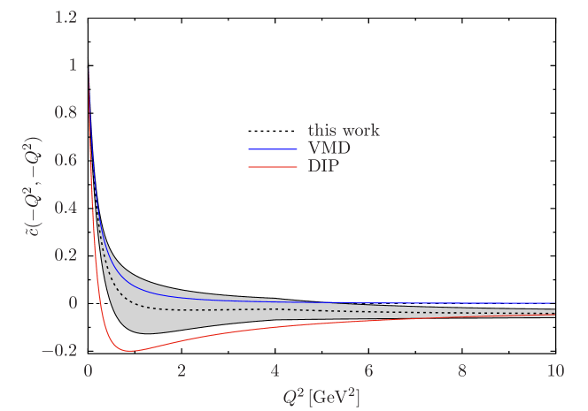
Figure 6: The normalized diagonal form factor $\tilde{c}(-Q^{2},-Q^{2})$ (black dashed line with uncertainty band), in comparison to the VMD model and the DIP parameterization D’Ambrosio et al. (1998).

It is instructive to compare our results for the LD contribution to previous evaluations. The simplest model, a VMD form factor with mass scale fit to reproduce the slope (19), gives

$$\text{Re}\,\mathcal{A}_{\mu}^{\text{LD, VMD}}(M_{K}^{2})=-0.68(11),\qquad\text{Re}\,\mathcal{A}_{e}^{\text{LD, VMD}}(M_{K}^{2})=31.36(26),$$ (97)

where the uncertainty is propagated from $b_{K_{L}}$. The corresponding diagonal form factor is compared to our result in Fig. 6, which shows that the main differences to the VMD model concern a faster decrease for small $Q^{2}$ and a negative asymptotic tail. While the dispersive part in Eq. (5.1) comes out similar to the VMD result, the asymptotic contribution entails a positive shift that brings the net result closer to the experimental value. Ultimately, this enhancement arises from logarithmic corrections that lead to an asymptotic behavior proportional to $\log Q^{2}/Q^{2}$, a feature that is absent in both the VMD and DIP models, with asymptotic limits proportional to $1/Q^{4}$ and $1/Q^{2}$, respectively.

For the DIP parameterization, with $\alpha_{\text{DIP}}=-1.69(8)$ from the global determination Workman et al. (2022) and $\beta_{\text{DIP}}=-1-2\alpha_{\text{DIP}}$ from the asymptotic constraint, one finds

$$\text{Re}\,\mathcal{A}_{\mu}^{\text{LD, DIP}}(M_{K}^{2})=0.57(28),\qquad\text{Re}\,\mathcal{A}_{e}^{\text{LD, DIP}}(M_{K}^{2})=32.46(71),$$ (98)

propagating the uncertainties from $\alpha_{\text{DIP}}$. The comparison to our result is again illustrated in Fig. 6, which shows that the higher central value of $\text{Re}\,\mathcal{A}_{\mu}(M_{K}^{2})$ is driven by a more pronounced minimum of $\tilde{c}(-Q^{2},-Q^{2})$ around $Q^{2}=1\,\text{GeV}^{2}$, more than compensating for the missing $\log Q^{2}$ in the asymptotic behavior and thereby even reversing the sign of the resulting value for $\text{Re}\,\mathcal{A}_{\mu}(M_{K}^{2})$. The corresponding low-energy constant $\chi_{\mu}^{\text{DIP}}(\mu)=5.70(28)$ comes out close to $\chi_{\mu}^{\text{\cite[cite]{\@@bibref{Authors Phrase1YearPhrase2}{Isidori:2003ts}{\@@citephrase{(}}{\@@citephrase{)}}}}}(\mu)=5.83(1.0)_{\text{th}}(0.15)_{\text{exp}}$. This central value was obtained in Ref. Isidori and Unterdorfer (2004) from a DIP parameterization with $\alpha_{\text{DIP}}=-1.611(44)$ and an expansion in $M_{K}$ and $m_{\mu}$. Using the same value for $\alpha_{\text{DIP}}$, but keeping the full loop integral, we find $\chi_{\mu}(\mu)=5.42(15)$ for this DIP contribution. The uncertainty is dominated by an estimate of high-energy contributions by varying a phenomenological ansatz within the range allowed by the partonic expression (59). In this work, we improved the matching to asymptotic constraints by separating the low- and high-energy parts of the loop functions via dispersion integrals, to the effect that the main uncertainty now arises from the RG corrections to the Wilson coefficients. However, the range for the high-energy contributions considered in Ref. Isidori and Unterdorfer (2004) does suggest a correction to the DIP solution in the direction of the VMD form factor, which is consistent with our findings and would move the value of the low-energy constant closer to Eq. (91).

6 Consequences for physics beyond the Standard Model

6.1 SMEFT

BSM constraints are most easily expressed in terms of the Wilson coefficients in

$${\mathcal{L}}^{\text{BSM}}=C_{A}^{\ell}\bar{s}\gamma^{\mu}\gamma_{5}d\,\bar{\ell}\gamma_{\mu}\gamma_{5}\ell+C_{P}^{\ell}\bar{s}i\gamma_{5}d\,\bar{\ell}i\gamma_{5}\ell+\text{h.c.},$$ (99)

leading to

$$\text{Re}\,\mathcal{A}_{\ell}^{\text{BSM}} =-\frac{4m_{\ell}F_{K}}{\mathcal{N}}\bigg{(}\text{Re}\,C_{A}^{\ell}+\frac{M_{K}^{2}}{2m_{\ell}(m_{s}+m_{d})}\text{Re}\,C_{P}^{\ell}\bigg{)}$$

$$=1.124(5)\times 10^{11}\,\text{GeV}^{2}\bigg{(}\text{Re}\,C_{A}^{\ell}+\frac{M_{K}^{2}}{2m_{\ell}(m_{s}+m_{d})}\text{Re}\,C_{P}^{\ell}\bigg{)},$$ (100)

where the normalization

$$\mathcal{N}=-\frac{\alpha}{\pi}\frac{m_{\ell}}{M_{K}}\sqrt{\frac{16\pi\Gamma[K_{L}\to\gamma\gamma]}{M_{K}}}$$ (101)

takes into account the relative sign compared to the LD contribution in the same conventions as in Sec. 4 and App. A (similar expressions are available in the literature, see, e.g., Refs. Mescia et al. (2006); Chobanova et al. (2018)). The axial-vector coefficient maps onto the Gilman–Wise basis Gilman and Wise (1979, 1980); Buras (1998)

$${\mathcal{L}}=-\frac{G_{F}}{\sqrt{2}}V_{us}^{*}V_{ud}C_{7A}^{\ell}\,\bar{s}\gamma^{\mu}(1-\gamma_{5})d\,\bar{\ell}\gamma_{\mu}\gamma_{5}\ell+\text{h.c.}$$ (102)

according to $C_{A}^{\ell}=\frac{G_{F}}{\sqrt{2}}V_{us}^{*}V_{ud}C_{7A}^{\ell}$, and the tree-level matching to SMEFT coefficients Grzadkowski et al. (2010); Buchmüller and Wyler (1986) reads

$$C_{A}^{\ell}=\frac{1}{4}\Big{(}C^{(1)}_{\ell q}+C^{(3)}_{\ell q}+C_{ed}-C_{\ell d}-C_{qe}\Big{)},\qquad C_{P}^{\ell}=-\frac{1}{4}C_{\ell edq},$$ (103)

with flavor indices $prst=\ell\ell 21$.

6.2 Modified $\boldsymbol{Z}$ couplings

A special case is given by the test of modified $Z$ couplings, defined by the effective Lagrangian Buras and Silvestrini (1999)

$${\mathcal{L}}=\frac{G_{F}}{\sqrt{2}}\frac{e}{2\pi^{2}}M_{Z}^{2}\frac{\cos\theta_{W}}{\sin\theta_{W}}Z_{ds}\,\bar{s}\gamma^{\mu}(1-\gamma_{5})d\,Z_{\mu},$$ (104)

which maps to

$$C_{A}^{\ell}=\frac{\alpha(M_{Z})G_{F}}{2\pi\sqrt{2}\,\sin^{2}\theta_{W}}Z_{ds}.$$ (105)

The SM contribution to $Z_{ds}$, corresponding to the last two diagrams in Fig. 2, gives $Z_{ds}=\lambda_{t}C_{0}(x_{t})$ Buchalla et al. (1991), and, together with the $W$ box, determines the SD part of $\chi(\mu)$ in Eq. (8). Choosing the sign in Eq. (95) in line with the SM, we obtain the constraint

$$\text{Re}\,Z_{ds}^{\text{BSM}}=1.6(5)_{\text{exp}}(8)_{\text{SM}}\times 10^{-4},\qquad|\text{Re}\,Z_{ds}^{\text{BSM}}|<2.8\times 10^{-4}\quad\text{at }90\%\text{ C.L.}$$ (106)

Limits on $\text{Re}\,Z_{ds}$ can also be extracted from $K^{+}\to\pi^{+}\nu\bar{\nu}$ Cortina Gil et al. (2021)

$$\text{Br}[K^{+}\to\pi^{+}\nu\bar{\nu}]\big{|}_{\text{NA62}}=\big{(}10.6^{+4.0}_{-3.4}\pm 0.9\big{)}\times 10^{-11},$$ (107)

which is sensitive to both the real and imaginary part of $Z_{ds}$ Buras and Silvestrini (1999); Buras et al. (2015); Brod et al. (2021)

$$\text{Br}[K^{+}\to\pi^{+}\nu\bar{\nu}] =\kappa_{+}\big{(}1+\Delta_{\text{EM}}\big{)}\bigg{[}\bigg{(}\frac{\text{Im}\,\lambda_{t}X_{t}+\text{Im}\,Z_{ds}^{\text{BSM}}}{\lambda^{5}}\bigg{)}^{2}$$

$$+\bigg{(}\frac{\text{Re}\,\lambda_{c}}{\lambda}\big{(}P_{c}+\delta P_{c,u}\big{)}+\frac{\text{Re}\,\lambda_{t}X_{t}+\text{Re}\,Z_{ds}^{\text{BSM}}}{\lambda^{5}}\bigg{)}^{2}\bigg{]}.$$ (108)

Evaluating the SM contribution with the input quantities summarized in Ref. Brod et al. (2021) (relying on Refs. Misiak and Urban (1999); Buchalla and Buras (1999); Isidori et al. (2005); Buras et al. (2006); Mescia and Smith (2007); Brod and Gorbahn (2008); Brod et al. (2011)), but with the CKM parameters as collected in App. A, we find $\text{Br}[K^{+}\to\pi^{+}\nu\bar{\nu}]|_{\text{SM}}=8.2(5)\times 10^{-11}$, in good agreement with Ref. Gorbahn (2023). Assuming $\text{Im}\,Z_{ds}^{\text{BSM}}=0$ and choosing again the sign that ensures agreement with the SM, we obtain

$$\text{Re}\,Z_{ds}^{\text{BSM}}=-1.1(1.5)_{\text{exp}}(0.2)_{\text{SM}}\times 10^{-4},\qquad|\text{Re}\,Z_{ds}^{\text{BSM}}|<3.1\times 10^{-4}\quad\text{at }90\%\text{ C.L.},$$ (109)

leading to a limit almost identical to Eq. (106). This observation nicely illustrates the complementarity of $K_{L}\to\mu^{+}\mu^{-}$ and $K^{+}\to\pi^{+}\nu\bar{\nu}$, since a combined analysis of the two processes can be used to disentangle BSM contributions to the real and imaginary part of $Z_{ds}$ at a similar level of precision. In view of the projected experimental advances for $K^{+}\to\pi^{+}\nu\bar{\nu}$ at NA62 and HIKE, this motivates commensurate efforts to improve the SM prediction for $K_{L}\to\mu^{+}\mu^{-}$ as well.

7 Summary and outlook

In this work, we analyzed the $K_{L}\to\gamma^{*}\gamma^{*}$ form factor in dispersion theory. To predict its low-energy part, we made use of data for $K_{L}\to\gamma\gamma$ and $K_{L}\to\ell^{+}\ell^{-}\gamma$, $K_{L}\to\ell_{1}^{+}\ell_{1}^{-}\ell^{+}_{2}\ell^{-}_{2}$ to determine normalization and slope, respectively, but, crucially, also for $K_{L}\to\pi^{+}\pi^{-}\gamma$, to constrain the $2\pi$ cuts in the spectral function for an isovector photon. Together with minimal narrow-width parameterizations for the isoscalar spectral functions as well as the $K^{*}\simeq K\pi$ contributions, we found that the resulting form factor, albeit mainly constrained by singly-virtual data, leaves remarkably little flexibility for doubly-virtual kinematics either. The representation for the full form factor was then supplemented by an asymptotic contribution, which derives from a dispersive formulation of the partonic calculation of $K_{L}\to\gamma^{*}\gamma^{*}$, to be able to separate low- and high-energy contribution by a suitable cutoff in the integrals. We observed that besides uncertainties in the dispersive representation and from the experimental value of the slope parameter, another important source of uncertainty arises from the perturbative running of the Wilson coefficients, which we studied including the resummation of subleading logarithms.

The central results are given in Eq. (5.1) for the real part of the long-distance amplitudes $\text{Re}\,\mathcal{A}_{\ell}(M_{K}^{2})$, and in Eq. (93) for the corresponding branching fractions. The sum of the long-distance amplitude for $K_{L}\to\mu^{+}\mu^{-}$ and the short-distance contribution in the SM agrees with experiment at the level of $1.7\sigma$, and the improved uncertainty in $\text{Re}\,\mathcal{A}_{\mu}(M_{K}^{2})$ allows us to formulate more stringent limits on physics beyond the SM. The uncertainty in the prediction of the long-distance contribution could be further improved if better data for the $K_{L}\to\pi^{+}\pi^{-}\gamma$ and $K_{L}\to\ell^{+}\ell^{-}\gamma$ spectra were available, this would allow one to reduce the dispersive uncertainty and the precision of the form-factor slope. In this context, we emphasize that it is unfortunate that the original data for the respective spectra from Refs. Abouzaid et al. (2007); Alavi-Harati et al. (2001a); Ramberg et al. (1993); Abouzaid et al. (2006) are not accessible, as, especially for the dilepton data, we are thus forced to rely on the quoted parameters for fits using a specific model for the form factor. While we tried to minimize the impact of the corresponding assumptions by constructing our dispersive parameterization in a way consistent with these fits, they could have been avoided altogether if the data for the spectra themselves had been preserved.

The asymptotic uncertainty could potentially be improved using the interplay with lattice QCD Christ et al. (2023); Zhao and Christ (2022); Christ et al. (2020), which could also help unambiguously determine the relative sign of long- and short-distance contributions. Further, it would be very helpful if lattice QCD could provide information on the relative weights between normalizations of different isospin currents, as this would allow one to test the vector-meson-dominance assumptions currently needed for the prediction of the doubly-virtual form factor. Already with the improvements implemented in this work, the final uncertainty in Eq. (92) is getting close to experiment (94), so that with future advances in theory it should become possible to match the current experimental precision, especially, if improved input for the $K_{L}\to\pi^{+}\pi^{-}\gamma$ and $K_{L}\to\ell^{+}\ell^{-}\gamma$ spectra became available. As we argued in Sec. 6, the corresponding constraints on physics beyond the Standard Model are complementary to the ones obtained from $K\to\pi\nu\bar{\nu}$, motivating further efforts to improve the SM prediction for $K_{L}\to\mu^{+}\mu^{-}$.

Appendix A Short-distance contribution in the Standard Model

Following Refs. Buchalla and Buras (1994); Gorbahn and Haisch (2006), the SD contribution in the SM can be expressed as

$$\text{Br}[K_{L}\to\mu^{+}\mu^{-}]\big{|}_{\text{SD}}=\kappa_{\mu}\bigg{[}\frac{\text{Re}\,\lambda_{t}}{\lambda^{5}}Y(x_{t})+\frac{\text{Re}\,\lambda_{c}}{\lambda}P_{c}\bigg{]}^{2},$$ (110)

where $\lambda_{i}=V_{is}^{*}V_{id}$ collects the CKM matrix elements, $\lambda=|V_{us}|$ denotes the Wolfenstein parameter, $Y(x_{t})$ is a loop function depending on the top quark $\overline{\text{MS}}$ mass via $x_{t}=[m_{t}(\mu_{t})]^{2}/M_{W}^{2}$ and the top quark matching scale $\mu_{t}$, and $P_{c}$ gives the contribution from the charm loop. The dependence on $\lambda$ is far less pronounced than Eq. (110) suggests, since the normalization

$$\kappa_{\mu}=\frac{[\alpha(M_{Z})]^{2}\text{Br}[K^{+}\to\mu^{+}\nu_{\mu}]}{\pi^{2}\sin^{4}\theta_{W}}\frac{\tau(K_{L})}{\tau(K^{+})}\lambda^{8}=1.999(9)\times 10^{-9}\bigg{(}\frac{\lambda}{0.225}\bigg{)}^{8}$$ (111)

together with the scaling $P_{c}\propto\lambda^{-4}$ cancels all but the remaining power $1/\lambda^{2}$ in $\text{Br}[K_{L}\to\mu^{+}\mu^{-}]$. For the numerical evaluation of Eq. (111) we use the global fit from Ref. Cirigliano et al. (2023),

$$\text{Br}[K^{+}\to\mu^{+}\nu_{\mu}]=63.58(11)\%,\qquad\tau(K^{+})=12.384(15)\,\text{ns},\qquad\tau(K_{L})=51.16(21)\,\text{ns},$$ (112)

as well as $\alpha(M_{Z})\equiv\alpha_{\overline{\text{MS}}}(M_{Z})=1/127.9$ and $\sin^{2}\theta_{W}\equiv\sin^{2}\hat{\theta}_{W}^{\overline{\text{MS}}}=0.23122(4)$ Workman et al. (2022). For the CKM matrix elements we use Workman et al. (2022); Vale Silva (2023)

$$\text{Re}\,\lambda_{c} =-\lambda\bigg{(}1-\frac{\lambda^{2}}{2}\bigg{)}=-0.2193(7),\qquad\lambda=0.2250(8),$$

$$\text{Re}\,\lambda_{t} =-A^{2}\lambda^{5}\bigg{(}1-\frac{\lambda^{2}}{2}\bigg{)}(1-\bar{\rho})=-3.21(11)\times 10^{-4},$$

$$A =0.824(11),\qquad\bar{\rho}=0.158(10),$$

$$\text{Im}\,\lambda_{t} =A^{2}\bar{\eta}\lambda^{5}\bigg{(}1+\frac{\lambda^{2}}{2}\bigg{)}=1.41(6)\times 10^{-4},\qquad\bar{\eta}=0.351(9),$$ (113)

where we have taken the mean of the numbers using CKMFitter Höcker et al. (2001); Charles et al. (2005) and UTfit Bona et al. (2005, 2008) methodology and assigned the respective larger error.

The loop function $Y(x_{t})$ has recently been updated in Ref. Brod and Stamou (2023), and we use the resulting value $Y(x_{t})=0.931(5)$. For $P_{c}$ we use the approximate formula given in Ref. Gorbahn and Haisch (2006) to update its value to $m_{c}(m_{c})=1.278(13)\,\text{GeV}$ Aoki et al. (2022); Carrasco et al. (2014); Alexandrou et al. (2014); Chakraborty et al. (2015); Bazavov et al. (2018a); Hatton et al. (2020) and $\alpha_{s}(M_{Z})=0.1184(8)$ Aoki et al. (2022); Chakraborty et al. (2015); Maltman et al. (2008); Aoki et al. (2009); McNeile et al. (2010); Bruno et al. (2017); Bazavov et al. (2019); Calì et al. (2020); Ayala et al. (2020), which results in

$$P_{c}=0.111(10)\bigg{(}\frac{0.225}{\lambda}\bigg{)}^{4}.$$ (114)

The error therein is dominated by the residual scale ambiguities at this order, to which we have added linearly the small remaining uncertainty $\Delta P_{c}=0.002$ due to $m_{c}$, see Ref. Gorbahn and Haisch (2006). Taking everything together, we obtain

$$\text{Br}[K_{L}\to\mu^{+}\mu^{-}]\big{|}_{\text{SD}}=0.784(55)\times 10^{-9},$$ (115)

which translates to the SD contribution

$$\chi_{\text{SD}}^{\text{SM}}=-1.804(64).$$ (116)

The uncertainty is completely dominated by the CKM matrix elements, with the largest contribution from the Wolfenstein parameter $A$.

An equivalent representation of $\chi_{\text{SD}}^{\text{SM}}$ was derived in Ref. Isidori and Unterdorfer (2004) starting from

$$C_{\text{SD}}^{\text{SM}}=-\frac{\sqrt{2}\,G_{F}\alpha(M_{Z})m_{\mu}F_{K}}{\pi\sin^{2}\theta_{W}}\Big{(}\text{Re}\,\lambda_{t}Y(x_{t})+\lambda^{4}\text{Re}\,\lambda_{c}P_{c}\Big{)},$$ (117)

which amounts to

$$\chi_{\text{SD}}^{\text{SM}} =-\tilde{\kappa}\Big{(}\text{Re}\,\lambda_{t}Y(x_{t})+\lambda^{4}\text{Re}\,\lambda_{c}P_{c}\Big{)}=-1.802(59),$$

$$|\tilde{\kappa}| =\sqrt{\frac{M_{K}}{16\pi\Gamma[K_{L}\to\gamma\gamma]}}\frac{\sqrt{2}\,G_{F}M_{K}F_{K}\alpha(M_{Z})}{\sin^{2}\theta_{W}\alpha(0)}=4988.4(23.6),$$ (118)

where we have used $G_{F}=1.1663788(6)\times 10^{-5}\,\text{GeV}^{-2}$ Workman et al. (2022); Tishchenko et al. (2013) and $F_{K}=110.58(24)\,\text{MeV}$ as additional inputs. The resulting value of $\chi_{\text{SD}}^{\text{SM}}$ is in good agreement with Eq. (116), motivating the final estimate quoted in Eq. (8). In both cases we have introduced a relative sign to account for the negative normalization of the $K_{L}\to\gamma\gamma$ amplitude, see Sec. 4.

Appendix B Dispersive representation of loop functions

B.1 Two-point function

The two-point function for quark flavor $q=u,c$ can be represented in the form

$$T_{q}(q^{2})=2\int_{0}^{1}\text{d}x\,x(1-x)\log\bigg{[}1-x(1-x)\frac{q^{2}}{m_{q}^{2}}\bigg{]},$$ (119)

and recast into the dispersive representation

$$T_{q}(q^{2})=\frac{q^{2}}{\pi}\int_{4m_{q}^{2}}^{\infty}\text{d}s\frac{\text{Im}\,T_{q}(s)}{s(s-q^{2})},$$ (120)

with

$$\text{Im}\,T_{q}(s)=-\frac{\pi}{3}\sigma_{q}(s)\bigg{(}1+\frac{2m_{q}^{2}}{s}\bigg{)}.$$ (121)

In the matching to short-distance constraints, we use a variant of Eq. (120) in which $m_{u}\to 0$ and lower cutoffs $s_{q}$ applied in the dispersion integrals, to separate the parts already accounted for via the low-energy contributions. This leads to

$$T_{c}^{\text{asym}}(q^{2})-T_{u}^{\text{asym}}(q^{2}) =-\frac{q^{2}}{3}\bigg{[}\int_{s_{c}}^{\infty}\text{d}s\frac{\sigma_{c}(s)(s+2m_{c}^{2})}{s^{2}(s-q^{2})}-\int_{s_{u}}^{\infty}\frac{\text{d}s}{s(s-q^{2})}\bigg{]}$$

$$=-\frac{1}{3}\bigg{[}\frac{5}{3}\big{(}1-\sigma_{c}(s_{c})\big{)}+\frac{4m_{c}^{2}}{q^{2}}\bigg{(}1-\sigma_{c}(s_{c})\Big{(}1+\frac{q^{2}}{3s_{c}}\Big{)}\bigg{)}$$

$$\quad+\frac{\sigma_{c}(q^{2})(q^{2}+2m_{c}^{2})}{q^{2}}\log\frac{\frac{\sigma_{c}(q^{2})+\sigma_{c}(s_{c})}{\sigma_{c}(q^{2})-\sigma_{c}(s_{c})}}{\frac{\sigma_{c}(q^{2})+1}{\sigma_{c}(q^{2})-1}}+\log\frac{s_{u}-q^{2}}{s_{u}}\bigg{]}$$

$$=-\frac{1}{3}\bigg{[}\frac{5}{3}\big{(}1-\sigma_{c}(s_{c})\big{)}-\frac{4m_{c}^{2}\sigma_{c}(s_{c})}{3s_{c}}+\log\frac{1+\sigma_{c}(s_{c})}{1-\sigma_{c}(s_{c})}-\log\frac{s_{u}}{m_{c}^{2}}\bigg{]}$$

$$\quad+\mathcal{O}\Big{(}\frac{1}{q^{2}}\Big{)},$$ (122)

written in a form that applies for space-like $q^{2}$ and expanded for asymptotic values in the last step. To ensure that the entire contribution drops as $1/q^{2}$, $s_{u}$ and $s_{c}$ therefore cannot be varied independently. In particular, one has $s_{u}>s_{c}$, e.g., for $s_{c}=4m_{c}^{2}$ one needs to set $s_{u}=\mathrm{e}^{5/3}m_{c}^{2}$.

B.2 Three-point function

In the literature, the three-point function is represented in the form Simma and Wyler (1990); Herrlich and Kalinowski (1992)

$$I_{q}(r_{1},r_{2},r_{3}) =\int_{0}^{1}\text{d}x\int_{0}^{1-x}\text{d}y\bigg{\{}\frac{2-x-y+(r_{1}x+r_{2}y)(1-x-y)^{2}+r_{3}xy(2-x-y)}{1-(r_{1}x+r_{2}y)(1-x-y)-r_{3}xy}$$

$$\quad-(2-3x-3y)\log\big{[}1-(r_{1}x+r_{2}y)(1-x-y)-r_{3}xy\big{]}\bigg{\}}-\frac{2}{3},$$ (123)

where $r_{1}=q_{1}^{2}/m_{q}^{2}$, $r_{2}=q_{2}^{2}/m_{q}^{2}$, $r_{3}=M_{K}^{2}/m_{q}^{2}$. Starting from this parameterization, we calculated the discontinuity in $r_{1}$, which takes a very simple form

$$\text{disc}_{r_{1}}I_{q}(r_{1},r_{2},r_{3})=-\frac{4\pi i\theta(r_{1}-4)}{\lambda^{1/2}_{123}}\log\frac{r_{1}-r_{2}-r_{3}-\sigma_{1}\lambda_{123}^{1/2}}{r_{1}-r_{2}-r_{3}+\sigma_{1}\lambda_{123}^{1/2}},$$ (124)

where $\lambda_{123}=\lambda(r_{1},r_{2},r_{3})$ and $\sigma_{1}=\sqrt{1-4/r_{1}}$. In particular, this expression coincides up to a factor $-2$ with the corresponding discontinuity of the scalar loop function

$$C_{0}(r_{1},r_{2},r_{3})=-\int_{0}^{1}\text{d}x\int_{0}^{1-x}\text{d}y\frac{1}{1-(r_{1}x+r_{2}y)(1-x-y)-r_{3}xy},$$ (125)

so that the difference to Eq. (B.2) can only arise from a subtraction polynomial. Indeed, we find that

$$I_{q}(r_{1},r_{2},r_{3})=-2C_{0}(r_{1},r_{2},r_{3})-1$$ (126)

holds in general, and will continue to work with this simplified expression. The loop function fulfills the limits

$$I_{q}(0,0,r_{3})=\frac{4}{r_{3}}\arctan^{2}\frac{\sqrt{r_{3}}}{\sqrt{4-r_{3}}}-1=\frac{r_{3}}{12}+\mathcal{O}\big{(}r_{3}^{2}\big{)}$$ (127)

and

$$I_{q}(r_{1},r_{2},r_{3})\big{|}_{r_{1},r_{2}\gg r_{3}\gg 1}=-1,\qquad I_{q}(r_{1},r_{2},r_{3})\big{|}_{r_{3}\gg r_{1},r_{2}\gg 1}=-\frac{1}{2}.$$ (128)

Using Eq. (124) for the discontinuity, we find the dispersive representation

$$I_{q}(r_{1},r_{2},r_{3})=-1+\frac{1}{2\pi i}\int_{4}^{\infty}\text{d}x\frac{\text{disc}_{r_{1}}I_{q}(x,r_{2},r_{3})}{x-r_{1}}.$$ (129)

Such a form can again be used to isolate low-energy contributions, i.e., by imposing a lower cutoff $s_{u}$, the limit $m_{u}\to 0$ can be taken, and only $I_{u}(r_{1},r_{2},r_{3})=-1$ remains. For the $c$-loop contribution, the single-variable dispersion relation suggests a form

$$I_{c}(q_{1}^{2},q_{2}^{2},M_{K}^{2})=-1+\frac{m_{c}^{2}}{\pi}\int_{s_{c}}^{\infty}\text{d}x\frac{2\pi\log\frac{x-q_{2}^{2}-M_{K}^{2}+\sigma_{c}(x)\lambda^{1/2}(x,q_{2}^{2},M_{K}^{2})}{x-q_{2}^{2}-M_{K}^{2}-\sigma_{c}(x)\lambda^{1/2}(x,q_{2}^{2},M_{K}^{2})}}{(x-q_{1}^{2})\lambda^{1/2}(x,q_{2}^{2},M_{K}^{2})}.$$ (130)

Such a form, however, does not strictly suffice to isolate the low-energy contributions, since the second variable $q_{2}^{2}$ can still take arbitrary values. For this reason, it is advantageous to formulate a double-spectral representation and impose cutoffs in both virtualities.

As a first step, we consider the limit $r_{3}=0$ of the discontinuity (124):

$$\text{disc}_{r_{1}}I_{q}(r_{1},r_{2},0)=\frac{4\pi i}{r_{1}-r_{2}}\log\frac{1+\sigma_{1}}{1-\sigma_{1}},\qquad\sigma_{1}=\sqrt{1-\frac{4}{r_{1}}}.$$ (131)

The corresponding double-spectral function becomes

$$\rho(r_{1},r_{2},0)=2\pi^{2}\delta(r_{1}-r_{2})\log\frac{1+\sigma_{1}}{1-\sigma_{1}},$$ (132)

leading to

$$I_{q}(r_{1},r_{2},0)=-1+\frac{1}{\pi^{2}}\int_{4}^{\infty}\text{d}x\int_{4}^{\infty}\text{d}y\frac{\rho(x,y,0)}{(x-r_{1})(y-r_{2})}.$$ (133)

Due to the $\delta$-function in Eq. (132), it is clear that support for the double-spectral integration only comes from the line $r_{1}=r_{2}$, which provides further motivation for imposing a cutoff only in the single-variable dispersion relation (129).

Next, we generalize Eq. (132) to non-zero values of $r_{3}$. The simplest case is $r_{3}<0$, admitting the representation

$$I_{q}(r_{1},r_{2},r_{3}) =-1+\frac{1}{\pi^{2}}\int_{4}^{\infty}\text{d}x\int_{4}^{\infty}\text{d}y\frac{\rho(x,y,r_{3})}{(x-r_{1})(y-r_{2})}$$

$$=-1+\frac{1}{\pi^{2}}\int_{4}^{\infty}\text{d}x\int_{r_{2}^{-}(x,r_{3})}^{r_{2}^{+}(x,r_{3})}\text{d}y\frac{2\pi^{2}}{(x-r_{1})(y-r_{2})\lambda^{1/2}(x,y,r_{3})},$$ (134)

with double-spectral function

$$\rho(r_{1},r_{2},r_{3})=\frac{2\pi^{2}}{\lambda^{1/2}_{123}}\theta(-\lambda_{123}-r_{1}r_{2}r_{3})$$ (135)

and corresponding integration boundaries

$$r_{2}^{\pm}(r_{1},r_{3})=r_{1}+r_{3}-\frac{r_{1}r_{3}}{2}\pm\frac{1}{2}\sqrt{r_{1}(r_{1}-4)r_{3}(r_{3}-4)}.$$ (136)

Unfortunately, a simple representation such as Eq. (B.2) only applies for $r_{3}<0$, otherwise, additional contributions from anomalous cuts need to be included Lucha et al. (2007); Hoferichter et al. (2014b); Colangelo et al. (2015). Such contributions arise because the branch points of $\lambda_{123}$,

$$r_{\pm}(r_{1},r_{3})=(\sqrt{r_{1}}\pm\sqrt{r_{3}})^{2},$$ (137)

can move through the cut between $r_{2}^{+}$ and $r_{2}^{-}$ onto the first sheet and require a deformation of the contour. In the case $0<r_{3}<4$, we find the representation

$$I_{q}(r_{1},r_{2},r_{3}) =-1-\frac{1}{\pi^{2}}\int_{4}^{\infty}\text{d}x\frac{2\pi^{2}}{x-r_{1}}\sum_{I=\pm}\int_{r_{-}(x,r_{3})}^{\tilde{r}_{2}^{I}(x,r_{3})}\text{d}y\frac{1}{(y-r_{2})\lambda^{1/2}(x,y,r_{3})},$$ (138)

where

$$\tilde{r}_{2}^{\pm}=r_{1}+r_{3}-\frac{r_{1}r_{3}}{2}\mp\frac{i}{2}\sqrt{r_{1}(r_{1}-4)r_{3}(4-r_{3})}$$ (139)

and the integration is performed along the straight line from $r_{-}$ to $\tilde{r}_{2}^{\pm}$. Inserting Heaviside functions $\theta(x-s_{c}/m_{c}^{2})$, $\theta(|y|-s_{c}/m_{c}^{2})$ into Eq. (138), we obtain an improved variant of Eq. (130) that removes the low-energy contributions below $s_{c}$ in both virtualities.

Finally, in the case $r_{3}>4$, as relevant for $q=u$, the $\tilde{r}_{2}^{\pm}$ become real again, but $\lambda^{1/2}(x,y,r_{3})$ produces imaginary parts that correspond to the decay $K\to\bar{u}u$. Such imaginary parts clearly need to be covered by the low-energy part of the representation and cannot be present in the asymptotic contribution. However, the scaling of the $u$-quark integral can already be read off from Eq. (133): introducing a cutoff $s_{u}$ in both integrations and evaluating the $\delta$-function, the remaining integral becomes

$$I_{u}(q_{1}^{2},q_{2}^{2},0)=-1+2\int_{s_{u}}^{\infty}\frac{\text{d}x}{(x-q_{1}^{2})(x-q_{2}^{2})}m_{u}^{2}\log\frac{1+\sigma_{u}(x)}{1-\sigma_{u}(x)}=-1+\mathcal{O}(m_{u}^{2}\log m_{u}),$$ (140)

since $s_{u}$ prevents a potential infrared singularity for $q_{1}^{2}=q_{2}^{2}=0$. Given that an analysis based on Eq. (138) yields the same scaling, we set $I_{u}(q_{1}^{2},q_{2}^{2},M_{K}^{2})=-1$.

Appendix C Integration kernels

The integration kernels for the evaluation of the loop integral (85) are given as

$$K(x) =\frac{2i}{\pi^{2}M_{K}^{2}}\int\text{d}^{4}k\frac{M_{K}^{2}k^{2}-(q\cdot k)^{2}}{(q-k)^{2}\big{[}(p-k)^{2}-m_{\ell}^{2}\big{]}}\times\frac{x}{x-k^{2}},$$ (141)

$$K(x,y) =\frac{2i}{\pi^{2}M_{K}^{2}}\int\text{d}^{4}k\frac{M_{K}^{2}k^{2}-(q\cdot k)^{2}}{k^{2}(q-k)^{2}\big{[}(p-k)^{2}-m_{\ell}^{2}\big{]}}\times\frac{xy}{(x-k^{2})\big{[}y-(q-k)^{2}\big{]}},$$

$$K(x,y,z) =\frac{2i}{\pi^{2}M_{K}^{2}}\int\text{d}^{4}k\frac{M_{K}^{2}k^{2}-(q\cdot k)^{2}}{k^{2}(q-k)^{2}\big{[}(p-k)^{2}-m_{\ell}^{2}\big{]}}\times\frac{xyz}{\big{(}x-k^{2}\big{)}\big{[}y-(q-k)^{2}\big{]}\big{(}z-k^{2}\big{)}}.$$

The asymptotic formula is given by Weil et al. (2017)

$$\text{Re}\,\mathcal{A}_{\ell}(M_{K}^{2}) =\mathcal{A}_{\ell}(0)+\frac{1}{\sigma_{\ell}(M_{K}^{2})}\bigg{[}\text{Li}_{2}\big{[}-y_{\ell}(M_{K}^{2})\big{]}+\frac{1}{4}\log^{2}\big{[}y_{\ell}(M_{K}^{2})\big{]}+\frac{\pi^{2}}{12}\bigg{]},$$

$$\mathcal{A}_{\ell}(0) =\frac{4}{3}\int_{0}^{\infty}\text{d}x\bigg{[}(x-2)\sqrt{1+\frac{1}{x}}-x+\frac{3}{2}\bigg{]}\tilde{c}^{\text{asym}}(-Q^{2},-Q^{2}),$$ (142)

where $x=Q^{2}/(4m_{\ell}^{2})$. We emphasize that this approximation is only used for the asymptotic contribution, for which we verified that the incurred error is negligible compared to the uncertainty in the RG evolution. For the low-energy contributions the difference to the full evaluation of the loop integral can be sizable, and we therefore keep the exact form in terms of the kernel functions (141).