Generative Fractional Diffusion Models

Abstract

We generalize the continuous time framework for score-based generative models from an underlying Brownian motion (BM) to an approximation of fractional Brownian motion (FBM). We derive a continuous reparameterization trick and the reverse time model by representing FBM as a stochastic integral over a family of Ornstein-Uhlenbeck processes to define generative fractional diffusion models (GFDM) with driving noise converging to a non-Markovian process of infinite quadratic variation. The Hurst index $H\in(0,1)$ of FBM enables control of the roughness of the distribution transforming path. To the best of our knowledge, this is the first attempt to build a generative model upon a stochastic process with infinite quadratic variation.

1 Introduction

Modeling the distribution transforming process of score-based generative models through stochastic differential equations (SDEs) in continuous time offers a unifying framework for data generation (Song et al., 2021). The underlying stochastic process of score matching with Langevin dynamics (SMLD) and denoising diffusion probabilistic modeling (DDPM) corresponds to a specific choice of $\mu$ and $\sigma$ in the dynamics

$$dX_{t}=\mu(t)X_{t}dt+\sigma(t)dW_{t},\quad X_{0}\sim\mathcal{D}$$ (1)

of the forward process driven by a Brownian motion $W$ with unknown data distribution $\mathcal{D}$. To sample data from noise an exact reverse time model is given by

$$d\overline{X}_{t}=\left[\overline{\mu}(t)\overline{X}_{t}-\overline{\sigma}^{2}(t)\nabla_{x}\log p_{T-t}(\overline{X}_{t})\right]dt+\overline{\sigma}(t)d\overline{W}_{t},\quad X_{T}\sim\mathcal{N}(0,I),$$ (2)

where only the score-function $\nabla_{x}\log p_{t}(x)$ is unknown. Extensive research has been carried out over the past years to examine (Karras et al., 2022; Chen et al., 2023; Singhal et al., 2023) and extend (Jing et al., 2022; Huang et al., 2022; Bunne et al., 2023; Song et al., 2023) the continuous time view on generative models through the lens of SDEs. A natural question is to ask whether a generalization from an underlying Brownian motion (BM) to a fractional Brownian motion (FBM) is possible. Since FBM is neither a Markov process nor a semimartingale (Biagini et al., 2008), Itô calculus (Itô, 1987) may not be applied to derive an analogous conditional backward Kolmogorov equation for the derivation of the reverse time model (Anderson, 1982). To overcome this difficulty we represent FBM as a stochastic integral over a family of Ornstein–Uhlenbeck (OU) processes and approximate FBM by a weighted sum of OU processes (Harms and Stefanovits, 2019) to define a score-based generative model with driving noise converging to FBM.

figurec

Figure 1: The Hurst index $H\in(0,1)$ controls the roughness of the forward process by varying the quadratic variation. The driving noise converges for $H<0.5$ to a process of infinite quadratic variation and for $H\geq 0.5$ to a process of finite quadratic variation.

2 Generative Fractional Diffusion Models

For simplicity, we assume one-dimensional data and refer to Appendix A for the multidimensional case and the mathematical details. We adapt the approach of Harms and Stefanovits (2019) to define the underlying noise process of our score-based generative model resulting in a Gaussian forward process that possesses an explicit formula for the mean and the variance of the marginal distribution w.r.t. to time. The reverse time model transforms into a system of coupled correlated processes.

2.1 Forward Model

Representing FBM with Hurst index $H\in(0,1)$ by the integral

$$W^{H}_{t}=\begin{cases}\int_{0}^{\infty}\left(Y^{x}_{t}-Y^{x}_{0}\right)\nu(dx),\quad&H\leq\frac{1}{2}\\ \int_{0}^{\infty}\left(Z^{x}_{t}-Z^{x}_{0}\right)\nu(dx),\quad&H>\frac{1}{2}\end{cases}$$ (3)

over the family of two dimensional OU processes $\left(Y^{x},Z^{x}\right)_{x\in\mathbb{R}}$ results in the approximation

$$W^{H}_{t}\approx W_{t}^{H,m}=\begin{cases}\int_{0}^{\infty}(Y^{x}_{t}-Y^{x}_{0})\nu^{m}(dx)=\sum_{i=1}^{m}q^{m}_{i}\left(Y^{x^{m}_{i}}_{t}-Y^{x^{m}_{i}}_{0}\right),\quad&H\leq\frac{1}{2}\\ \int_{0}^{\infty}(Z^{x}_{t}-Z^{x}_{0})\nu^{m}(dx)=\sum_{i=1}^{m}q^{m}_{i}\left(Z^{x^{m}_{i}}_{t}-Z^{x^{m}_{i}}_{0}\right),\quad&H>\frac{1}{2}.\end{cases}$$ (4)

For $H=\frac{1}{2}$, we retrieve $W^{\frac{1}{2}}_{t}=\int_{0}^{\infty}\left(Y^{x}_{t}-Y^{x}_{0}\right)\delta_{0}(dx)=Y_{t}^{0}-Y^{0}_{0}=W_{t}$ the purely Brownian setting of the Variance Exploding (VE), the Variance Preserving (VP) and the sub-VP dynamics of Song et al. (2021). For Lipschitz continuous drift and diffusion functions $\mu,\sigma:[0,T]\to\mathbb{R}$ define the forward process $X=(X_{t})_{t\in[0,T]}$ of the generative fractional diffusion model (GFDM) by

$$dX_{t}=\mu(t)X_{t}dt+\sigma(t)dW_{t}^{H,m},\quad X_{0}=x_{0}\sim\mathcal{D}.$$ (5)

Analogous to the discrete reparameterization trick $X_{t_{n}}=\sqrt{\bar{\alpha}_{t_{n}}}x_{0}+\sqrt{1-\bar{\alpha}_{t_{n}}}\bm{\epsilon},\epsilon\sim\mathcal{N}(\bm{0},\bm{I})$ used in DDPM (Ho et al., 2020), we show by reparameterizing the forward process and applying the Stochastic Fubini Theorem (Harms and Stefanovits, 2019) that the forward process conditioned on the data sample $x_{0}$ is a Gaussian process,

Continuous Reparameterization Trick.

The forward process $X$ of GFDM conditioned on $X_{0}=x_{0}\in\mathbb{R}$ admits the continuous reparameterization $X_{t}=c(t)(x_{0}+\int_{0}^{t}\alpha(t,s)dW_{s})$ such that $X$ is a Gaussian process with $X_{t}\sim\mathcal{N}(c(t)x_{0},\sigma^{2}_{t})$ and $\sigma^{2}_{t}=c^{2}(t)\int^{t}_{0}\alpha^{2}(t,s)ds$.

For the proof see Theorem 1 in Section A.3. The continuous reparameterization enables to directly sample from the conditional forward process of GFDM at any $t\in(0,T]$ and bypasses the need to solve a differential equation to calculate the mean and the variance of the corresponding marginal distribution. In accordance with Song et al. (2021) we present three specifications of GFDM and call the dynamics of GFDM.

Fractional Variance Exploding (FVE) if the process $X$ follows the dynamics

$$dX_{t}=\sqrt{\frac{d\left[\sigma^{2}(t)\right]}{dt}}dW_{t}^{H,m}\quad\textit{with}\quad\sigma(t)=\sigma_{min}\frac{\sigma_{max}}{\sigma_{T}}\left(\frac{\sigma_{max}}{\sigma_{min}}\right)^{t},$$ (6)

where $0<\sigma_{min}<\sigma_{max}$ are determined by Technique 1 of Song and Ermon (2020).

Fractional Variance Preserving (FVP) if the process $X$ adheres to the dynamics

$$dX_{t}=-\frac{1}{2}\beta(t)X_{t}dt+\sqrt{\beta(t)}dW_{t}^{H,m}\quad\textit{with}\quad\beta(t)=\bar{\beta}_{\min}+t\left(\bar{\beta}_{max}-\bar{\beta}_{min}\right)$$ (7)

and $\beta_{min}=0.1,\beta_{max}=20$ match the setting of Ho et al. (2020).

Sub-Fractional Variance Preserving (sub-FVP) if the process $X$ solves

$$dX_{t}=-\frac{1}{2}\beta(t)X_{t}dt+\sqrt{\beta(t)\left(1-e^{-2\int_{0}^{t}\beta(s)ds}\right)}dW_{t}^{H,m}.$$ (8)

2.2 Reverse Time Model

An application of Ito’s formula (Itô, 1987) to the linear combination $W^{H,m}$ of OU processes results in the forward dynamics

$$dX_{t}=\left[\mu(t)X_{t}-\sigma(t)S^{H}_{t}\right]dt+C_{H}\sigma(t)dW_{t},\quad X_{0}\sim\mathcal{D}$$ (9)

and we realize that GFDM is already contained in the general framework of Song et al. (2021) but differs in the dynamics and the dimensionality from VE, VP, and sub-VP by the additional processes $S^{H}$ defined in eq. 27. Since $W^{H,m}$ approximates a process with the correlation function $\rho_{H}(t,s)=\frac{1}{2}\left[t^{2H}+s^{2H}-|t-s|^{2H}\right]$ corresponding to FBM (Harms and Stefanovits, 2019), the additional process $S^{H}$ introduces a shift in variance and correlation w.r.t. the time $t\in[0,T]$. Since we aim to study the effect of correlation and not the effect of a differing variance schedule, we normalize the terminal variance of FVE, FVP, and sub-FVP to the terminal variance for $H=\frac{1}{2}$ corresponding to VE, VP, and sub-VP. See Figure 4 in Appendix B for an illustration of the resulting variance evolution over time and the shift in correlation. The reverse time model transforms for $H\not=\frac{1}{2}$ to a coupled system of reverse time models.

Time Reversal.

The one-dimensional reverse time model of GFDM is given by the coupled dynamics

$$d\overline{X}_{t} =\left[\overline{\mu}(t)\overline{X}_{t}-\overline{\sigma}(t)\overline{S^{H}}_{t}-\sum^{m}_{i=1}\overline{G^{H}_{i}}(t)\nabla_{v}\log p_{i}\left(\overline{V^{i}}_{t},T-t\right)\right]dt+c_{H}\overline{\sigma}(t)d\overline{W}_{t}$$ (10)

$$d\overline{Y}^{i}_{t} =\left[-x^{i}\overline{Y}^{i}_{t}-\overline{F^{H}_{i}}(t)\nabla_{v}\log p_{i}\left(\overline{V}^{i}_{t},T-t\right)\right]dt+d\overline{W}_{t},\quad i=1,...,m$$ (11)

$$d\overline{Z^{i}}_{t} =\left[-x^{i}\overline{Z^{i}}_{t}+\overline{Y^{i}}_{t}\right]dt,\quad i=1,...,m.$$ (12)

with $V^{i}=(X^{i},Y^{i},Z^{i})$, where the vector-valued functions $\overline{G^{H}_{i}},\overline{F^{H}_{i}}:[0,T]\to\mathbb{R}^{d,2d}$ are defined by

$$\overline{G^{H}_{i}}(T-t)=\mathbbm{1}_{(0,\frac{1}{2}]}(H)\begin{pmatrix}q^{2}_{i}\sigma^{2}(t)&q_{i}\sigma(t)\\ \end{pmatrix}\quad\textit{and}\quad\overline{F^{H}_{i}}(T-t)=\begin{pmatrix}\mathbbm{1}_{(0,\frac{1}{2}]}(H)q_{i}\sigma(t)&1\\ \end{pmatrix}.$$ (13)

Due to the correlation of the coupled reverse dynamics we obtain the score functions $\nabla_{v^{i}}\log p_{1},...,\nabla_{v^{i}}\log p_{m}$ in the dynamics of the reverse time model by rescaling the score function $\nabla_{x}p(\cdot,t)$ of $X_{t}$ according to the derivation in Section A.4. To approximate $\nabla_{x}p(\cdot,t)$ we train a time-dependent score-based model $s_{\theta}$ aiming for $\theta^{\star}=\operatorname*{arg\,min}_{\theta}\mathbb{E}\lambda(t)\left\|s_{\theta}(X_{t},t)-\xi/\sigma_{t}\right\|^{2}_{2}$ where $\xi\sim\mathcal{N}(0,1)$, $\lambda:[0,T]\to(0,\infty)$ is a positive weighting function, $t\sim\mathcal{U}[0,T]$, $X_{0}\sim\mathcal{D}$ and $X_{t}\sim\mathcal{N}(m_{t},\sigma^{2}_{t})$ is conditioned on $x_{0}$.

3 Experiments

(a) Visualization of the sampling methods ability to generate data from the swiss roll dataset distribution with a data noise value of $0.1$.

(b) Visualization of the sampling methods ability to generate the half moon dataset distribution with a data noise value of $0.01$.

Figure 2: Visualized are the learned data distributions for varying $H$ and different sampling methods.

Table 1: Quantitative results for the swiss roll dataset.

	$H$	WSD $\downarrow$		IP $\uparrow$		IR $\uparrow$		VS $\uparrow$
		FVP	S.FVP	FVP	S.FVP	FVP	S.FVP	FVP	S.FVP
SDE	0.01	0.018	0.020	0.614	0.955	0.993	0.975	1.999	1.998
	0.25	0.020	0.022	0.705	0.953	0.990	0.973	1.999	1.998
	0.5	0.021	0.027	0.871	0.967	0.983	0.965	1.999	1.997
gSDE	0.01	0.061	0.063	0.602	0.969	0.991	0.960	1.997	1.997
	0.25	0.053	0.053	0.703	0.964	0.991	0.966	1.997	1.998
	0.5	-	-	-	-	-	-	-	-
nODE	0.01	0.126	0.135	0.968	0.985	0.951	0.941	1.986	1.988
	0.25	0.162	0.172	0.983	0.992	0.920	0.913	1.979	1.968
	0.5	0.020	0.020	0.940	0.964	0.971	0.970	1.999	2.00

We test the ability of GFDM to sample from a two-dimensional distribution for varying $H\in\{0.01,0.25,0.5\}$. To foster comparability we use a fixed random seed for training and the exact same U-Net, i.e. we use the same initialization of weights. During sampling, the same realisation of the underlying standard normal distributed noise vectors are used across all $H$ to simulate the reverse time model and we average all computed metrics over five sampling runs. For the qualitative evaluation of the generated data we compute the mean wasserstein distance (WSD) (Arjovsky et al., 2017) of the two dimensions, the improved precision (IP) and the improved recall (IR) (Kynkäänniemi et al., 2019). To evaluate the diversity of the generated samples we use the vendi score (VS) (Friedman and Dieng, 2022). The additional processes for $H<\frac{1}{2}$ enable us to define guided SDE (gSDE) sampling and noisy ODE (nODE) sampling. In gSDE we use in the SDE for the simulation of $\overline{X}$ and the probability flow ODE for $\overline{Y^{1}},...,\overline{Y^{m}}$ while nODE deploys the probability flow ODE for $X$ and the SDE for $\overline{Y^{1}},...,\overline{Y^{m}}$. For $H=\frac{1}{2}$ gSDE and nODE reduces to sampling from the SDE and the probability flow ODE. See Appendix C for details of the sampling procedure and Appendix E for additional results. In Table 1 we observe that the initial model for $H=0.5$ reaches the highest score only for sub-FVP dynamics in terms of a WSD of $0.020$. The sampling method nODE performs particulary well for $H=0.25$ in terms of an IP of $0.983$ for FVP and $0.992$ for sub-VP. For SDE sampling the roughest model performs best in terms of a WSD and IR, at the cost of a low IP of $0.614$. Even though we averaged the scores over five runs and used the same noise realisation accross varying $H$ we want to point out that the differences in the scores are mostly very small. Nevertheless the Hurst index seems to have an influence on the ability to approximate the true data distrbution and nODE sampling appears to be a promising sampling method.

4 Discussion and Outlook

In this work, we determined the extent to which the continuous time framework of score-based generative models can be generalized to FBM. We identified challenges and proposed an approach that leverages the representation of FBM by a stochastic integral over a family of OU processes (Harms and Stefanovits, 2019) that results in an explicit formula for the marginal distribution of the forward process w.r.t. time. For $H\not=\frac{1}{2}$ the reverse time model transforms to a coupled system of correlated reverse time models, thus enabling the definition of sampling methods using a mixture of SDE and probability flow ODE dynamics. The proposed methods show promising results on two-dimensional data.

The framework presented in this work can be expanded. Besides the investigation of $H>\frac{1}{2}$, a particularly interesting extension of the proposed GFDM is the approach to define a diffusion model in space and time (sketched in Section A.5), in order to use infinitely many correlation scales for training.

Appendix A The Framework of Generative Fractional Diffusion Models

In this section we provide the mathematical details of generative fractional diffusion models presented in the main paper. The driving noise of the generative model is based on the affine representation of fractional processes from Harms and Stefanovits [2019]. We begin with the definition of the underlying stochastic processes.

A.1 Definition of the Underlying Stochastic Processes

Let $(\Omega,\mathcal{F},\mathbb{P})$ be a complete probability space equipped with a complete and right continuous filtration $\{\mathcal{F}_{t}\}$. For two independent $\{\mathcal{F}_{t}\}$-Brownian motions (BM) $W^{1}$, $W^{2}$ a two-sided $\{\mathcal{F}_{t}\}$-BM is defined by

$$W_{t}:=\begin{cases}W_{t}=W^{1}_{t},\quad t\geq 0\\ W_{t}=W^{2}_{-t}\quad\textit{otherwise}.\end{cases}$$ (14)

The process

$$W^{H}_{t}:=\frac{1}{\Gamma(H+\frac{1}{2})}\int_{-\infty}^{0}((t-s)^{H-\frac{1}{2}}-(-s)^{H-\frac{1}{2}})dW_{s}+\frac{1}{\Gamma(H+\frac{1}{2})}\int_{0}^{t}(t-s)^{H-\frac{1}{2}}dW_{s}$$ (15)

is called fractional Brownian motion (FBM) with Hurst index $H\in(0,1)$ [Mandelbrot and Van Ness, 1968], defining the family $(W^{H})_{H\in(0,1)}$ of centered Gaussian processes [Biagini et al., 2008] with covariance function

$$\rho_{H}(t,s)=\frac{1}{2}\left[t^{2H}+s^{2H}-|t-s|^{2H}\right],\quad t\geq s>0.$$ (16)

Brownian motion, being the unique continuous and centered Gaussian process with covariance function $\rho_{\frac{1}{2}}(t,s)=t\land s$, is recovered for $H=\frac{1}{2}$ [Biagini et al., 2008]. For $H\in(0,1)\setminus\{\frac{1}{2}\}$ the process possesses correlated increments and, for $H\in(0,\frac{1}{2})$, infinite quadratic variation [Rogers, 1997] such that $W^{H}$ is neither a Markov-process nor a semimartingale [Biagini et al., 2008]. Hence, Itô calculus and in particular the results from Anderson [1982] may not be applied to derive a reverse time model for a process driven by $W^{H}$. In Appendix F we describe these difficulties in more detail. To circumvent this problem, we approximate FBM as a finite sum of weighted Markovian semimartingales according to Harms and Stefanovits [2019]. To prepare this approximation, define for every $x\in(0,\infty)$ the pair $(Y_{t}^{x},Z_{t}^{x})_{t\geq 0}$ of Ornstein-Uhlenbeck processes

$$Y^{x}_{t}=Y^{x}_{0}e^{-tx}+\int_{0}^{t}e^{-(t-s)x}dW_{s},\quad Z^{x}_{t}=Z^{x}_{0}e^{-tx}+Y^{x}_{0}e^{-tx}+\int_{0}^{t}(t-s)e^{-(t-s)x}dW_{s}$$ (17)

with the speed of mean reversion $x$ and starting values

$$\quad Y_{0}=\int_{-\infty}^{0}e^{sx}dW_{s},\quad Z_{0}=\int_{-\infty}^{0}se^{sx}dW_{s}.$$ (18)

By Itôs product rule [Cohen and J.Elliott, 2015], the processes $(Y_{t}^{x},Z_{t}^{x})_{t\geq 0}$ solve the stochastic differential equation (SDE)

$$dY^{x}_{t}=-xY^{x}_{t}dt+dW_{t},\quad dZ_{t}=(-xZ_{t}+Y_{t})dt;$$ (19)

see [Harms and Stefanovits, 2019, Remark 2.2].

A.2 Markovian Representation of Fractional Brownian Motion

Define the measure $\nu$ according to Harms and Stefanovits [2019] by

$$\nu(dx)=\begin{cases}\delta_{0},\quad&H=\frac{1}{2}\\ \frac{dx}{x^{\frac{1}{2}+H}\Gamma\left(H+\frac{1}{2}\right)\Gamma\left(\frac{1}{2}-H\right)},\quad&H<\frac{1}{2}\\ \frac{dx}{x^{H-\frac{1}{2}}\Gamma\left(H+\frac{1}{2}\right)\Gamma\left(\frac{3}{2}-H\right)},\quad&H>\frac{1}{2}\end{cases}$$ (20)

where $\delta_{0}$ is the Dirac measure supported on $0$. Theorem 3.5 in Harms and Stefanovits [2019] yields the infinite-dimensional Markovian representations

$$W^{H}_{t}=\begin{cases}\int_{0}^{\infty}\left(Y^{x}_{t}-Y^{x}_{0}\right)\nu(dx),\quad&H\leq\frac{1}{2}\\ \int_{0}^{\infty}\left(Z^{x}_{t}-Z^{x}_{0}\right)\nu(dx),\quad&H>\frac{1}{2}.\end{cases}$$ (21)

of FBM by an integral over the Markovian semimartingales $Y^{x}$ and $Z^{x}$. Note that for $H=\frac{1}{2}$ we retrieve

$$W^{\frac{1}{2}}_{t}=\int_{0}^{\infty}\left(Y^{x}_{t}-Y^{x}_{0}\right)\delta_{0}(dx)=Y_{t}^{0}-Y^{0}_{0}=W_{t},$$ (22)

such that Equation 21 holds true for BM as well. To derive an approximation of the above integrals by a finite sum, we follow the derivations presented in Bäuerle and Desmettre [2020] that are based on Carmona et al. [2000]. For a fixed geometric space grid $0<\xi^{m}_{0}<...<\xi^{m}_{m}$ of $m\in\mathbb{N}$ points set

$$x^{m}_{i+1}=\frac{\int_{\xi^{m}_{i}}^{\xi^{m}_{i+1}}x\nu(dx)}{\int_{\xi^{m}_{i}}^{\xi^{m}_{i+1}}\nu(dx)}\quad\textit{and}\quad q_{i+1}^{m}=\int_{\xi^{m}_{i}}^{\xi^{m}_{i+1}}\nu(dx),\quad 0\leq i\leq m-1$$ (23)

with corresponding measure $\nu^{m}=\sum_{i=1}^{m}q^{m}_{i}\delta_{x^{m}_{i}}$. For the detailed derivations of the above space grid quantities see Appendix D. The process

$$W_{t}^{H,m}=\begin{cases}\int_{0}^{\infty}(Y^{x}_{t}-Y^{x}_{0})\nu^{m}(dx)=\sum_{i=1}^{m}q^{m}_{i}\left(Y^{x^{m}_{i}}_{t}-Y^{x^{m}_{i}}_{0}\right),\quad&H\leq\frac{1}{2}\\ \int_{0}^{\infty}(Z^{x}_{t}-Z^{x}_{0})\nu^{m}(dx)=\sum_{i=1}^{m}q^{m}_{i}\left(Z^{x^{m}_{i}}_{t}-Z^{x^{m}_{i}}_{0}\right),\quad&H>\frac{1}{2}.\end{cases}$$ (24)

approximates $W^{H}$ with strong convergence rates of arbitrarily high polynomial order [Harms, 2019]. To ease notation we assume in the following a fixed $m\in\mathbb{N}$ and write $\xi_{i}=\xi^{m}_{i},q_{i}=q^{m}_{i},x_{i}=x^{m}_{i},Y^{i}=Y^{x^{m}_{i}}$ and $Z^{i}=Z^{x^{m}_{i}}$. Since we aim to study the path properties of a generative model based on $W^{H,m}$, we replace for simplification eq. 18 by $Y^{x}_{0}=Z^{x}_{0}=0$. The process $W^{H,m}$ enables us to define a score-based generative models with driving noise converging to FBM.

A.3 The Forward Model

Let $\bm{W}=\left(W_{1},...,W_{d}\right)$ be a $d$-dimensional two sided BM and $\bm{W}^{H,m}$ a $d$-dimensional vector valued stochastic process driven by $\bm{W}$ with entries $W^{H,m}_{1},...,W^{H,m}_{d}$ defined according to eq. 4. For Lipschitz continuous functions $\mu:[0,T]\to\mathbb{R}$ and $\sigma:[0,T]\to\mathbb{R}$ we define the forward process $\bm{X}=(\bm{X}_{t})_{t\in[0,T]}$ of a generative fractional diffusion model (GFDM) by

$$d\bm{X}_{t}=\mu(t)\bm{X}_{t}dt+\sigma(t)d\bm{W}^{H,m}_{t},\quad\bm{X}_{0}=\bm{x}_{0}\sim\mathcal{D},$$ (25)

where $\mathcal{D}$ is an unknown data distribution from which we aim to sample from. The forward process of GFDM approximates a score-based generative model driven by FBM, since $W^{H,m}\to W^{H}$ with convergence rates of arbitrarily high polynomial order [Harms, 2019]. Using the definition of $\bm{W}^{H,m}_{t}$ and eq. 19, the forward dynamics of GFBM can be written as

$$d\bm{X}_{t}=\left[\mu(t)\bm{X}_{t}-\sigma(t)\bm{S}^{H}_{t}\right]dt+C_{H}\sigma(t)d\bm{W}_{t},\quad\bm{X}_{0}=\bm{x}_{0}\sim\mathcal{D},$$ (26)

where $C_{H}=\mathbbm{1}_{(0,\frac{1}{2}]}(H)\sum^{m}_{i=1}q_{i}$ and $\bm{S}^{H}_{t}=(S^{H}_{t,1},...,S^{H}_{t,d})$ is the vector valued stochastic process

$$S^{H}_{t,j}=\begin{cases}\sum^{m}_{i=1}q_{i}x_{i}Y^{i}_{t,j},\quad&H\leq\frac{1}{2}\\ \sum^{m}_{i=1}q_{i}\left(x_{i}Z^{i}_{t,j}-Y^{i}_{t,j}\right),\quad&H>\frac{1}{2}.\end{cases}$$ (27)

The forward process of GFDM depends on additional processes resulting in a drift function that is no longer linear w.r.t. the state of the process. For that reason we can not follow [Song et al., 2021, Appendix B], to derive the perturbation kernel $p_{t}(\cdot|x_{0})$ corresponding to $\bm{X}_{t}$ conditioned on $\bm{x}_{0}$. Instead, we reparameterize the forward process resulting in an explicit formula for the mean and the variance.

Theorem 1 (Continuous Reparameterization Trick).

Let $\bm{x_{0}}$ be a fixed realisation drawn from $\mathcal{D}$. The forward process $\bm{X}=(\bm{X}_{t})_{t\in[0,T]}$ of GFDM can be reparameterized to

$$\bm{X}_{t}=c(t)\left(x_{0}+\int_{0}^{t}\alpha(t,s)d\bm{W}_{s}\right)$$ (28)

with $c(t)=\exp\left(\int_{0}^{t}\mu(s)ds\right)$ and

$$\alpha(t,s)=\begin{cases}-\sum_{i=1}^{m}q_{i}x_{i}\int_{s}^{t}\frac{\sigma(u)}{c(u)}e^{-x_{i}(u-s)}du+C_{H}\frac{\sigma(s)}{c(s)},\quad&H\leq\frac{1}{2}\\ -\sum_{i=1}^{m}q_{i}\int_{s}^{t}\frac{\sigma(u)}{c(u)}e^{-x_{i}(u-s)}\left[x_{i}(u-s)-1\right]du,\quad&H>\frac{1}{2}.\end{cases}$$ (29)

such that $\bm{X}_{t}\sim\mathcal{N}(\bm{m}_{t},\sigma^{2}_{t}\bm{I})$ is a Gaussian random vector for all $t\in(0,T]$ with

$$\bm{m}_{t}=c(t)\bm{x}_{0}\quad\textit{and}\quad\sigma^{2}_{t}=c^{2}(t)\int_{0}^{t}\alpha^{2}(t,s)ds.$$ (30)

Sketch of Proof.

Using the definition of $W_{t}^{H,m}$, one can rewrite the dynamics of the forward process as $dX_{t}=\left[\mu(t)X_{t}-\sigma(t)S^{H}_{t}\right]dt+C_{H}\sigma(t)dW_{t}$ where $S^{H}$ is a weighted sum of OU processes arising from Equation 4. Applying the Stochastic Fubini Theorem [Harms and Stefanovits, 2019] to a reparameterization of the forward process $X$ results in $X_{t}=c(t)\left(x_{0}+\int_{0}^{t}\alpha(t,s)dW_{s}\right)$. Since the integrand is deterministic, the integral w.r.t. Brownian motion is Gaussian, and we conclude that $X$ is Gaussian as well with $X_{t}\sim\mathcal{N}\left(c(t)x_{0},c^{2}(t)\int^{t}_{0}\alpha^{2}(t,s)ds\right)$. ∎

Proof.

By continuity, the functions $\mu$ and $\sigma$ are bounded. Moreover, the processes $(Y^{i}_{j},Z^{i}_{j})$ posses continuous, hence bounded, paths and thus

$$\int_{0}^{t}|\mu(u)|du<\infty,\quad\int_{0}^{t}\sigma^{2}(u)du<\infty\quad\textit{and}\quad\int_{0}^{t}|\bm{S}^{H}_{u}|du<\infty\quad\mathbb{P}-a.s.,$$ (31)

where the last integral is understood entrywise. Hence, by Theorem 16.6.1 in Cohen and J.Elliott [2015], the unique solution of the SDE eq. 26 is given explicitly as

$$\bm{X}_{t}=c(t)\left(\bm{x}_{0}-\int_{0}^{t}\frac{\sigma(u)}{c(u)}\bm{S}^{H}_{u}du+C_{H}\int_{0}^{t}\frac{\sigma(u)}{c(u)}d\bm{W}_{u}\right),\quad c(t)=\exp\left(\int_{0}^{t}\mu(s)ds\right).$$ (32)

By the definition of $(Y^{i}_{j},Z^{i}_{j})$ in (17) and the assumption $Y^{1}_{0}=Z^{1}_{0},...,=Y^{m}_{0}=Z^{m}_{0}=0$ we calculate by the Stochastic Fubini Theorem [Harms and Stefanovits, 2019, Theorem 6.1] for $H\leq\frac{1}{2}$

$$\int_{0}^{t}\frac{\sigma(u)}{c(u)}\bm{S}^{H}_{u}du =\sum_{i=1}^{m}q_{i}x_{i}\int_{0}^{t}\int_{0}^{u}\frac{\sigma(u)}{c(u)}e^{-x_{i}(u-s)}d\bm{W}_{s}du$$ (33)

$$=\int_{0}^{t}\sum_{i=1}^{m}q_{i}x_{i}\int_{s}^{t}\frac{\sigma(u)}{c(u)}e^{-x_{i}(u-s)}dud\bm{W}_{s},$$ (34)

and similarly for $H>\frac{1}{2}$

$$\int_{0}^{t}\frac{\sigma(u)}{c(u)}\bm{S}^{H}_{u}du =\sum_{i=1}^{m}q_{i}\int_{0}^{t}\int_{0}^{u}\frac{\sigma(u)}{c(u)}e^{-x_{i}(u-s)}\left[x_{i}(u-s)-1\right]d\bm{W}_{s}du$$ (35)

$$=\int_{0}^{t}\sum_{i=1}^{m}q_{i}\int_{s}^{t}\frac{\sigma(u)}{c(u)}e^{-x_{i}(u-s)}\left[x_{i}(u-s)-1\right]dud\bm{W}_{s}.$$ (36)

Hence, with

$$s^{H}_{i}(u,s)=\begin{cases}x_{i},\quad&H\leq\frac{1}{2}\\ x_{i}(u-s)-1&H>\frac{1}{2}\end{cases}$$ (37)

we calculate

$$\bm{X}_{t} =c(t)\left(\bm{x}_{0}-\int_{0}^{t}\frac{\sigma(u)}{c(u)}\bm{S}^{H}_{u}du+C_{H}\int_{0}^{t}\frac{\sigma(u)}{c(u)}d\bm{W}_{u}\right)$$ (38)

$$=c(t)\left(\bm{x}_{0}-\int_{0}^{t}\sum_{i=1}^{m}q_{i}\int_{s}^{t}\frac{\sigma(u)}{c(u)}e^{-x_{i}(u-s)}s^{H}_{i}(u,s)dud\bm{W}_{s}+C_{H}\int_{0}^{t}\frac{\sigma(u)}{c(u)}d\bm{W}_{u}\right)$$ (39)

$$=c(t)\left(\bm{x}_{0}+\int_{0}^{t}\left[-\sum_{i=1}^{m}q_{i}\int_{s}^{t}\frac{\sigma(u)}{c(u)}e^{-x_{i}(u-s)}s_{i}(u,s)du+C_{H}\frac{\sigma(s)}{c(s)}\right]d\bm{W}_{s}\right)$$ (40)

$$=c(t)\bm{x}_{0}+c(t)\int_{0}^{t}\alpha(t,s)d\bm{W}_{s},$$ (41)

where

$$\alpha(t,s)=\begin{cases}-\sum_{i=1}^{m}q_{i}x_{i}\int_{s}^{t}\frac{\sigma(u)}{c(u)}e^{-x_{i}(u-s)}du+C_{H}\frac{g(s)}{c(s)},\quad&H\leq\frac{1}{2}\\ -\sum_{i=1}^{m}q_{i}\int_{s}^{t}\frac{\sigma(u)}{c(u)}e^{-x_{i}(u-s)}\left[x_{i}(u-s)-1\right]du,\quad&H>\frac{1}{2}.\end{cases}$$ (42)

Since $\alpha(t,\cdot)$ is continuous for every fixed $t\in[0,T]$ we have $\int^{t}_{0}\alpha^{2}(t,s)ds<\infty$. Hence, conditional on $\bm{x}_{0}$, the random vector $\bm{X}_{t}\sim\mathcal{N}(\bm{m}_{t},\bm{\Sigma}_{t})$ is Gaussian with mean vector

$$\bm{m}_{t}=c(t)\bm{x}_{0}=\bm{x}_{0}\exp\left(\int_{0}^{t}\mu(s)ds\right).$$ (43)

and entrywise variance

$$\sigma^{2}_{t,j}=c^{2}(t)\int_{0}^{t}\alpha^{2}(t,s)ds.$$ (44)

Since the entries of $\bm{W}$ are independent, we find the covariance matrix

$$\bm{\Sigma}_{t}=\sigma^{2}_{t}\bm{I}\quad\textit{with}\quad\sigma^{2}_{t}=\sigma^{2}_{t,1}=...=\sigma^{2}_{t,j}.$$ (45)

∎

An application to the setting of Song et al. [2021] is straightforward for any linear drift function w.r.t. the state of the process and any diffusion function that does not depend on the state of the process. For example in the variance preserving (VP) setting corresponding to DDPM we have $H=\frac{1}{2}$, such that $m=1$ and $W_{t}^{H,m}=W_{t}^{H,1}=Y^{0}_{t}-Y_{0}=W_{t}$ results in $\alpha(t,s)=\exp\left(-\frac{1}{2}\int_{0}^{s}\beta(u)du\right)\sqrt{\beta(s)}$ for all $t\in[0,T]$ and hence eq. 28 reduces to

$$\bm{X}_{t}=\exp\left(-\frac{1}{2}\int^{t}_{0}\beta(u)du\right)\left(\bm{x}_{0}+\int_{0}^{t}\frac{\sqrt{\beta(s)}}{\exp\left(-\frac{1}{2}\int^{s}_{0}\beta(u)du\right)}d\bm{W}_{s}\right).$$ (46)

Using that the integral w.r.t. BM has zero mean, Continuous Reparameterization Trick enables us to directly calculate the mean

$$\mathbb{E}\left[\bm{X}_{t}\right]=\exp\left(-\frac{1}{2}\int^{t}_{0}\beta(u)du\right)\bm{x}_{0}$$ (47)

and the variance

$$\mathbb{V}\left[\bm{X}_{t}\right] =\exp\left(-\int^{t}_{0}\beta(u)du\right)\int^{t}_{0}\exp\left(\int^{s}_{0}\beta(u)du\right)\beta(s)ds$$ (48)

$$=\exp\left(-\int^{t}_{0}\beta(u)du\right)\left[\exp\left(\int^{s}_{0}\beta(u)du\right)\right]_{0}^{t}$$ (49)

$$=\exp\left(-\int^{t}_{0}\beta(u)du\right)\left[\exp\left(\int^{t}_{0}\beta(u)du\right)-1\right]$$ (50)

$$=1-\exp\left(-\int^{t}_{0}\beta(u)du\right)$$ (51)

in accordance with [Song et al., 2021, Equation (29)]. Note further that the above theorem generalizes the reparameterization trick used in Ho et al. [2020] from discrete time to continuous time in the sense that for example in setting of DDPM the reparameterization trick

$$\bm{X}_{t_{n}}=\sqrt{\bar{\alpha}_{t_{n}}}\bm{x}_{0}+\sqrt{1-\bar{\alpha}_{t_{n}}}\bm{\epsilon},\quad\bm{\epsilon}\sim\mathcal{N}(\bm{0},\bm{I})$$ (52)

with discrete time steps $0=t_{0}<...<t_{N}=T$ is replaced by the continuous time reparameterization

$$\bm{X}_{t}=c(t)\left(\bm{x}_{0}+\int^{t}_{0}\alpha(s)d\bm{W}_{s}\right).$$ (53)

The following corollary of the preceding theorem simplifies the derivation of the reverse time model in Section A.4. We show that the three-dimensional random vector $(X^{i}_{t,j},Y^{i}_{t,j},Z^{i}_{t,j})$ is trivariate normal distributed and derive the corresponding covariance matrix.

Corollary 2.

Let $\bm{X}^{i}$ be the solution of

$$d\bm{X}^{i}_{t}=\begin{cases}\mu(t)\bm{X}^{i}_{t}dt-q_{i}x_{i}\sigma(t)\bm{Y}^{i}_{t}dt+q_{i}\sigma(t)d\bm{W}_{t},&H\leq\frac{1}{2},\\ \mu(t)\bm{X}^{i}_{t}dt-q_{i}\sigma(t)\left[x_{i}\bm{Z}^{i}_{t}-\bm{Y}^{i}_{t}\right]dt,&H>\frac{1}{2},\end{cases}\quad\bm{X}^{i}_{0}=\frac{\bm{x}_{0}}{m}$$ (54)

for a fixed $i\in\{1,...,m\}$. The random vector $\bm{V}_{t}^{i}=(X^{i}_{t,1},Y^{i}_{t,1},Z^{i}_{t,1}),\dots,(X^{i}_{t,d},Y^{i}_{t,d},Z^{i}_{t,d})$ is multivariate normal for any $t\in[0,T]$. The corresponding covariance matrix is given by the block matrix

$$\bm{\Sigma}^{i}_{t}=diag\left(\bm{\Sigma}^{i}_{t,1},...,\bm{\Sigma}^{i}_{t,d}\right),$$ (55)

where $\bm{\Sigma}^{i}_{t,j}$ is the covariance matrix of the trivariate normal distributed random vector $(X^{i}_{t,j},Y^{i}_{t,j})$.

Proof.

For $j=1,\dots,d$ fixed, similarly to Theorem 1, Theorem 16.6.1 in Cohen and J.Elliott [2015] implies that we have the explicit representations

$$X^{i}_{t,j} =c(t)\left(\frac{x_{0}}{m}+\int^{t}_{0}\alpha_{i}(t,s)dW_{s,j}\right)$$ (56)

$$Y^{i}_{t,j} =\int^{t}_{0}e^{-x_{i}(t-s)}dW_{s,j},$$ (57)

$$Z^{i}_{t,j} =\int_{0}^{t}(t-s)e^{-x_{i}(t-s)}dW_{s,j},$$ (58)

where

$$\alpha_{i}(t,s)=\begin{cases}-q_{i}x_{i}\int_{s}^{t}\frac{\sigma(u)}{c(u)}e^{-x_{i}(u-s)}du+q_{i}\frac{\sigma(s)}{c(s)},\quad&H\leq\frac{1}{2},\\ -q_{i}\int_{s}^{t}\frac{\sigma(u)}{c(u)}e^{-x_{i}(u-s)}\left[x_{i}(u-s)-1\right]du,\quad&H>\frac{1}{2}.\end{cases}$$ (59)

We now use that the three normal random variables $X^{i}_{t,j}$, $Y^{i}_{t,j}$, and $Z^{i}_{t,j}$ are trivariate normal if and only if any linear combination of the three random variables is univariate normal. Let therefore $a_{1},a_{2},a3\in\mathbb{R}$, and note that

$$a_{1}X^{i}_{t,j}+a_{2}Y^{i}_{t,j}+a_{3}Z^{i}_{t,j}\\ =a_{1}c(t)\frac{x_{0}}{m}+\int^{t}_{0}a_{1}c(t)\alpha_{i}(t,s)+a_{2}e^{-x_{i}(t-s)}+a_{3}(t-s)e^{-x_{i}(t-s)}dW_{s,j},$$ (60)

showing that $a_{1}X^{i}_{t,j}+a_{2}Y^{i}_{t,j}+a_{3}Z^{i}_{t,j}$ is univariate normal. Therefore, $(X^{i}_{t,j},Y^{i}_{t,j},Z^{i}_{t,j})$ is trivariate normal. Finally, since the BMs $W_{t,1},\dots,W_{t,d}$ are independent, so are the pairs $(X^{i}_{t,1},Y^{i}_{t,1},Z^{i}_{t,1}),\dots,(X^{i}_{t,d},Y^{i}_{t,d},Z^{i}_{t,d})$, and hence $\bm{V}^{i}_{t}$ is multivariate normal with covariance matrix

$$\bm{\Sigma}^{i}_{t}=diag\left(\bm{\Sigma}^{i}_{t,1},...,\bm{\Sigma}^{i}_{t,d}\right),$$ (61)

where $\bm{\Sigma}^{i}_{t,j}$ is the covariance matrix of the trivariate normal vector $(X^{i}_{t,j},Y^{i}_{t,j},Z^{i}_{t,j})$ given by

$$\begin{pmatrix}\int_{0}^{t}c^{2}(t)\alpha_{i}^{2}(t,s)ds&\int_{0}^{t}c(t)\alpha_{i}(t,s)e^{-x_{i}(t-s)}ds&\int_{0}^{t}(t-s)c(t)\alpha_{i}(t,s)e^{-x_{i}(t-s)}ds\\ \int_{0}^{t}c(t)\alpha_{i}(t,s)e^{-x_{i}(t-s)}ds&\int_{0}^{t}e^{-2x_{i}(t-s)}ds&\int_{0}^{t}(t-s)e^{-2x_{i}(t-s)}ds\\ \int_{0}^{t}(t-s)c(t)\alpha_{i}(t,s)e^{-x_{i}(t-s)}ds&\int_{0}^{t}(t-s)e^{-2x_{i}(t-s)}ds&\int_{0}^{t}(t-s)^{2}e^{-2x_{i}(t-s)}ds.\end{pmatrix}$$ (62)

∎

A.4 The Reverse Time Model

The preceding Theorem 1 enables the derivation of the reverse time model using Anderson [1982]. In fact, we note by eq. 28 that the forward dynamics of GFDM is already contained in the framework of Song et al. [2021], but differs in the dynamics from VE, VP and sub-VP, since the forward process depends on the additional processes $\bm{S}^{H}$. To derive the reverse time model, we need to reverse the coupled dynamics of $\bm{X}$ and $\bm{S}^{H}$. In what follows, whenever $\bm{P}=(\bm{P}_{t})_{t\in[0,T]}$ is a stochastic process and $f$ is a function on $[0,T]$, we write $\overline{\bm{P}}_{t}=\bm{P}_{T-t}$ for the reverse time model and $\overline{f}(t)=f(T-t)$ for the reverse time function, respectively. Following Anderson [1982] we present the reverse time model of GFDM and derive the corresponding loss function to train a time-dependent score-based model aiming to approximate the following dynamics.

Theorem 3 (Time Reversal).

The reverse time model of the forward process $\bm{X}$ of GFDM is given by the coupled dynamics

$$d\overline{\bm{X}}_{t} =\left[\overline{\mu}(t)\overline{\bm{X}}_{t}-\overline{\sigma}(t)\overline{\bm{S}^{H}}_{t}-\sum^{m}_{i=1}\overline{G^{H}_{i}}(t)\nabla_{v}\log p_{i}\left(\overline{\bm{V}^{i}}_{t},T-t\right)\right]dt+c_{H}\overline{\sigma}(t)d\overline{\bm{W}}_{t}$$ (63)

$$d\overline{\bm{Y}}^{i}_{t} =\left[-x^{i}\overline{\bm{Y}}^{i}_{t}-\overline{F}^{H}_{i}(t)\nabla_{v}\log p_{i}\left(\overline{\bm{V}}^{i}_{t},T-t\right)\right]dt+d\overline{\bm{W}}_{t},\quad i=1,...,m$$ (64)

$$d\overline{\bm{Z}^{i}}_{t} =\left[-x^{i}\overline{\bm{Z}^{i}}_{t}+\overline{\bm{Y}^{i}}_{t}\right]dt,\quad i=1,...,m.$$ (65)

with $\bm{V}^{i}=(X^{i}_{1},Y^{i}_{1},Z^{i}_{1},X^{i}_{2},Y^{i}_{2},Z^{i}_{2}...,X^{i}_{d},Y^{i}_{d},Z^{i}_{d})$, where the matrix valued functions $\overline{G^{i}},\overline{F}^{i}:[0,T]\to\mathbb{R}^{d,2d}$ are defined by

$$\overline{G^{i}}(T-t)=\mathbbm{1}_{(0,\frac{1}{2}]}(H)\begin{pmatrix}q^{2}_{i}\sigma^{2}(t)&q_{i}\sigma(t)&0&\dots&0\\ 0&q^{2}_{i}\sigma^{2}(t)&q_{i}\sigma(t)&\dots&0\\ \vdots&\ddots&\ddots&\ddots&0\\ 0&\dots&0&q^{2}_{i}\sigma^{2}(t)&q_{i}\sigma(t)\\ \end{pmatrix}$$ (66)

and

$$\overline{F}^{i}(T-t)=\begin{pmatrix}\mathbbm{1}_{(0,\frac{1}{2}]}(H)q_{i}\sigma(t)&1&0&\dots&0\\ 0&\mathbbm{1}_{(0,\frac{1}{2}]}(H)q_{i}\sigma(t)&1&\dots&0\\ \vdots&\ddots&\ddots&\ddots&0\\ 0&\dots&0&\mathbbm{1}_{(0,\frac{1}{2}]}(H)q_{i}\sigma(t)&1\\ \end{pmatrix}.$$ (67)

Sketch of Proof.

Define functions $f_{i}^{H},R^{H}_{i}$ such that $d\bm{V}_{t}^{i}=f_{i}(\bm{V}_{t}^{i},t)dt+R^{H}_{i}(t)d\bm{W}_{t}$ and apply Anderson [1982] to derive the reverse time model $\overline{\bm{V^{i}}}$ of $\bm{V^{i}}$ for all $i=1,...,m$. This yields the reverse time model of GFDM since $\bm{X}_{t}=\sum_{i=1}^{m}\bm{X}^{i}_{t}$. ∎

Proof.

Fix $i\in\{1,...,m\}$ and define $\bm{V}_{t}^{i}=(X^{i}_{t,1},Y^{i}_{t,1},Z^{i}_{t,1},...,X^{i}_{t,d},Y^{i}_{t,d},Z^{i}_{t,d})$ according to Corollary 2. Let $f_{i}^{H}:\mathbb{R}^{3d}\times[0,T]\to\mathbb{R}^{3d}$ be the function

$$[f^{H}_{i}(v,t)]_{3j-2} =\mu(t)v_{3j-2}-q_{i}\sigma(t)s^{H}(t,v_{3j-1},v_{3j}),$$ (68)

$$[f^{H}_{i}(v,t)]_{3j-1} =-x_{i}v_{3j-1},$$ (69)

$$[f^{H}_{i}(v,t)]_{3j} =-x_{i}v_{3j}+v_{3j-1},$$ (70)

for $j=1,\dots,d$, where

$$s_{i}^{H}(t,v_{3j-1},v_{3j})=\begin{cases}x_{i}v_{3j-1}&H\leq\frac{1}{2},\\ x_{i}v_{3j}-v_{3j-1}&H>\frac{1}{2}.\end{cases}$$ (71)

We define $R^{H}_{i}:[0,T]\to\mathbb{R}^{3d,d}$ by

$$R^{H}_{i}(t)=\begin{pmatrix}1_{(0,1/2]}(H)q_{i}\sigma(t)&0&0&\dots&0\\ 1&0&0&\dots&0\\ 0&0&0&\dots&0\\ 0&1_{(0,1/2]}(H)q_{i}\sigma(t)&0&\dots&0\\ 0&1&0&\dots&0\\ 0&0&0&\dots&0\\ \vdots&\ddots&\ddots&\ddots&0\\ 0&\dots&0&0&1_{(0,1/2]}(H)q_{i}\sigma(t)\\ 0&\dots&0&0&1\\ 0&\dots&0&0&0\\ \end{pmatrix}\in\mathbb{R}^{3d,d}$$ (72)

such that

$$d\bm{V}_{t}^{i}=f_{i}(\bm{V}_{t}^{i},t)dt+R^{H}_{i}(t)d\bm{W}_{t},\quad i=1,...,m.$$ (73)

Following Anderson [1982], the reverse time model $\overline{\bm{V}^{i}}$ of $\bm{V}^{i}$ is given by

$$d\overline{\bm{V}_{t}^{i}}=\overline{f^{H}_{i}}\left(\overline{\bm{V}_{t}^{i}},t\right)dt-\overline{R^{H}_{i}}(t)\overline{R^{H}_{i}}(t)^{T}\nabla_{v}\log\left(p_{i}\left(\overline{\bm{V}_{t}^{i}},T-t\right)\right)dt+\overline{R^{H}_{i}}(t)d\overline{\bm{W}}_{t}$$ (74)

with $\overline{R_{i}^{H}}(t)\overline{R_{i}^{H}}(t)^{T}=diag\left(A^{H}(T-t),...,A^{H}(T-t)\right)$ where

$$A^{H}(t)=\begin{pmatrix}1_{(0,1/2]}(H)q_{i}^{2}\sigma^{2}(t)&1_{(0,1/2]}(H)q_{i}\sigma(t)&0\\ 1_{(0,1/2]}(H)q_{i}\sigma(t)&1&0\\ 0&0&0\end{pmatrix}.$$ (75)

Reordering of the entries using $u_{i}(\bm{X}_{t}^{i},\bm{Y}_{t}^{i},\bm{Z}_{t}^{i},t)=([f_{i}(\bm{V}_{t}^{i},t)]_{3j-2})_{j=1,\dots,d}$ and

$$\overline{G^{H}_{i}}(T-t)=\mathbbm{1}_{(0,\frac{1}{2}]}(H)\begin{pmatrix}q^{2}_{i}\sigma^{2}(t)&q_{i}\sigma(t)&0&\dots&0&0\\ 0&q^{2}_{i}\sigma^{2}(t)&q_{i}\sigma(t)&\dots&0&0\\ \vdots&\ddots&\ddots&\ddots&0&0\\ 0&\dots&0&q^{2}_{i}\sigma^{2}(t)&q_{i}\sigma(t)&0\\ \end{pmatrix}$$ (76)

as well as

$$\overline{F}^{H}_{i}(T-t)=\begin{pmatrix}\mathbbm{1}_{(0,\frac{1}{2}]}(H)q_{i}\sigma(t)&1&0&\dots&0&0\\ 0&\mathbbm{1}_{(0,\frac{1}{2}]}(H)q_{i}\sigma(t)&1&\dots&0&0\\ \vdots&\ddots&\ddots&\ddots&0&0\\ 0&\dots&0&\mathbbm{1}_{(0,\frac{1}{2}]}(H)q_{i}\sigma(t)&1&0\\ \end{pmatrix}$$ (77)

results in the coupled dynamics

$$d\overline{\bm{X}^{i}}_{t} =\left[\overline{u}(\overline{{\bm{X}}^{i}}_{t},\overline{\bm{Y}^{i}}_{t},\overline{\bm{Z}^{i}}_{t},t)-\overline{G^{H}_{i}}(t)\nabla_{v}\log p_{i}\left(\overline{\bm{V}^{i}}_{t},T-t\right)\right]dt+\mathbbm{1}_{(0,\frac{1}{2}]}(H)q_{i}\overline{\sigma}(t)d\overline{\bm{W}}_{t}$$ (78)

$$d\overline{\bm{Y}^{i}}_{t} =\left[-x^{i}\overline{\bm{Y}^{i}}_{t}-\overline{F^{H}_{i}}(t)\nabla_{v}\log p_{i}\left(\overline{\bm{V}^{i}}_{t},T-t\right)\right]dt+d\overline{\bm{W}}_{t}$$ (79)

$$d\overline{\bm{Z}^{i}}_{t} =\left[-x^{i}\overline{\bm{Z}^{i}}_{t}+\overline{\bm{Y}^{i}}_{t}\right]dt.$$ (80)

Since

$$\sum_{i=1}^{m}\bm{X}^{i}_{t}=x_{0}+\int^{t}_{0}\mu(u)\sum^{m}_{i=1}\bm{X}^{i}_{u}du-\int^{t}_{0}\sigma(u)\bm{S}^{H}_{u}du+c_{H}\int^{t}_{0}\sigma(u)d\bm{W}_{u}$$ (81)

solves eq. 26 of the forward process of GFDM we have $\overline{\bm{X}}_{t}=\sum_{i=1}^{m}\overline{\bm{X}^{i}}_{t}$ and the reverse time model of GFDM is given by the coupled dynamics

$$d\overline{\bm{X}}_{t} =\left[\overline{\mu}(t)\overline{\bm{X}}_{t}-\overline{\sigma}(t)\overline{\bm{S}^{H}}_{t}-\sum^{m}_{i=1}\overline{G^{H}_{i}}(t)\nabla_{v}\log p_{i}\left(\overline{\bm{V}^{i}}_{t},T-t\right)\right]dt+c_{H}\overline{\sigma}(t)d\overline{\bm{W}}_{t}$$ (82)

$$d\overline{\bm{Y}}^{i}_{t} =\left[-x^{i}\overline{\bm{Y}}^{i}_{t}-\overline{F}^{H}_{i}(t)\nabla_{v}\log p_{i}\left(\overline{\bm{V}}^{i}_{t},T-t\right)\right]dt+d\overline{\bm{W}}_{t},\quad i=1,...,m$$ (83)

$$d\overline{\bm{Z}^{i}}_{t} =\left[-x^{i}\overline{\bm{Z}^{i}}_{t}+\overline{\bm{Y}^{i}}_{t}\right]dt,\quad i=1,...,m.$$ (84)

∎

Note that if $H\leq 1/2$, the components related to $\bm{Z}$ vanish in the dynamics of the reverse time model and the distribution of $\bm{V}^{i}_{j}$ reduces from a trivariate normal distribution to a bivariate normal distribution. For the case $H\leq\frac{1}{2}$ we aim to train a time-dependent score-based model $s_{\theta}$ to approximate the dynamics of the reverse time model in order to generate samples from an approximate data distribution $\hat{\mathcal{D}}\approx\mathcal{D}$. However, a straightforward application of Song et al. [2021] would require to train $m$ models $s^{1}_{\theta},...,s^{m}_{\theta}$ w.r.t. the loss function

$$\tilde{L}(\bm{V}^{1}_{t},...,\bm{V}^{m}_{t},t,\theta)=\sum_{i=1}^{m}\mathbb{E}\left[\lambda(t)\|-\nabla_{v}\log p_{i}(\bm{V}^{i}_{t},t|\bm{v}_{0})-s^{i}_{\theta}(\bm{V}^{i}_{t},t)\|^{2}_{2}\right]$$ (85)

where $\lambda:[0,T]\to\mathbb{R}$ is a positive weighting function and the input dimension of the score-based model increases from $d$ to $2d$. To simplify the loss function we note by Corollary 2 that $p_{i}$ is the density of a multivariate normal distribution and we calculate for the $(2j-1)$-th and $2j$-th entry of the score function $\nabla_{\bm{v}^{i}}\log p_{i}(\cdot|\bm{v}^{i}_{0})$ the gradients

$$\left[\nabla_{\bm{v}^{i}}\log p_{i}(\bm{v}^{i},t|\bm{v}^{i}_{0})\right]_{2j-1}=-\frac{1}{2}\nabla_{x^{i}_{j}}\begin{pmatrix}x^{i}_{j}-m^{i}_{t,j},y^{i}_{j}\end{pmatrix}\left[\bm{\Sigma}^{i}_{t,j}\right]^{-1}\begin{pmatrix}x^{i}_{j}-m^{i}_{t,j}\\ y^{i}_{j}\\ \end{pmatrix}$$ (86)

and

$$\left[\nabla_{\bm{v}^{i}}\log p_{i}(\bm{v}^{i},t|\bm{v}^{i}_{0})\right]_{2j}=-\frac{1}{2}\nabla_{y^{i}_{j}}\begin{pmatrix}x^{i}_{j}-m^{i}_{t},y^{i}_{j}\end{pmatrix}\left[\bm{\Sigma}^{i}_{t,j}\right]^{-1}\begin{pmatrix}x^{i}_{j}-m^{i}_{t,j}\\ y^{i}_{j}\\ \end{pmatrix}$$ (87)

where we used from Corollary 2 that the covariance matrix of $\bm{V}^{i}_{t}$ is given by the block matrix

$$\bm{\Sigma}^{i}_{t}=diag\left(\bm{\Sigma}^{i}_{t,1},...,\bm{\Sigma}^{i}_{t,d}\right).$$ (88)

The above gradients are the gradients of the bivariate normal distribution corresponding to the $2$-dimensional vector $(X^{i}_{t,j},Y^{i}_{t,j})$ with density

$$q_{i}(x,y,t) =\frac{1}{Q_{i}(t)}\exp\left(-\frac{1}{2(1-\rho_{i}^{2}(t))}\left[\left(\frac{x-m_{t}}{\sigma_{t,i}}\right)^{2}-\frac{2\rho_{i}(t)(x-m_{t})y}{\sigma_{t,i}\tau_{t,i}}+\left(\frac{y}{\tau_{t,i}}\right)^{2}\right]\right),$$ (89)

where $\tau^{2}_{t,i}$ is the variance of $Y^{i}_{t,j}$, $Q_{i}(t)=2\pi\sigma_{t,i}\tau_{t,i}\sqrt{1-\rho_{i}^{2}(t)}$ is the normalizing constant and the correlation function $\rho_{i}$ is given by

$$\rho_{i}(t)=\frac{\langle X^{i}_{\cdot},Y^{i}_{\cdot}\rangle_{t}}{\sigma_{t,i}\tau_{t,i}}=\frac{1}{\sigma_{t,i}\tau_{t,i}}c(t)\int^{t}_{0}\alpha_{i}(t,s)e^{-x_{i}(t-s)}ds$$ (90)

since

$$\langle X^{i}_{\cdot},Y^{i}_{\cdot}\rangle_{t}=\left\langle c(t)\int^{\cdot}_{0}\alpha_{i}(\cdot,s)dW_{s},\int^{\cdot}_{0}e^{-x_{i}(\cdot-s)}dW_{s}\right\rangle_{t}=c(t)\int^{t}_{0}e^{-x_{i}(t-s)}\alpha_{i}(t,s)ds.$$ (91)

Hence, the derivatives in eq. 86 and eq. 87 are

$$\left[\nabla_{\bm{v}^{i}}\log p_{i}(\bm{v}^{i},t|\bm{v}^{i}_{0})\right]_{2j-1}=\nabla_{x}\log q_{i}(x,y,t)=-\frac{1}{1-\rho_{i}^{2}(t)}\left[\frac{x-m_{t}}{\sigma^{2}_{t,i}}-\rho_{i}(t)\frac{y}{\sigma_{t,i}\tau_{t,i}}\right]$$ (92)

and

$$\left[\nabla_{\bm{v}^{i}}\log p_{i}(\bm{v}^{i},t|\bm{v}^{i}_{0})\right]_{2j}=\nabla_{y}\log q_{i}(x,y,t)=-\frac{1}{1-\rho_{i}^{2}(t)}\left[-\frac{\rho_{i}(t)(x-m_{t})}{\sigma_{t,i}\tau_{t,i}}+\frac{y}{\tau^{2}_{t,i}}\right].$$ (93)

With $\bm{X}^{i}_{t}=\sigma_{t,i}\bm{\xi}+\bm{m}_{t}$, $\bm{Y}^{i}=\tau_{t,i}\bm{\xi}$ and $\bm{\xi}\sim\mathcal{N}(\bm{0}_{d},\bm{I}_{d})$ we note

$$\left[\nabla_{v}\log p_{i}(\bm{V}^{i}_{t},t|\bm{v}^{i}_{0})\right]_{2j-1}\stackrel{{\scriptstyle d}}{{=}}-\frac{1}{1-\rho_{i}^{2}(t)}\left[\frac{\xi_{j}}{\sigma_{t,i}}-\rho_{i}(t)\frac{\xi_{j}}{\sigma_{t,i}}\right]=-\frac{\xi_{j}}{(1+\rho_{i}(t))\sigma_{t,i}}$$ (94)

and

$$\left[\nabla_{v}\log p_{i}(\bm{V}^{i}_{t},t|\bm{v}^{i}_{0})\right]_{2j}\stackrel{{\scriptstyle d}}{{=}}-\frac{1}{1-\rho_{i}^{2}(t)}\left[-\frac{\rho_{i}(t)\xi_{j}}{\tau_{t,i}}+\frac{\xi_{j}}{\tau_{t,i}}\right]=-\frac{\xi_{j}}{(1+\rho_{i}(t))\tau_{i,t}}$$ (95)

such that

$$\left[\nabla_{v}\log p_{i}(\bm{V}^{i}_{t},t|\bm{v}^{i}_{0})\right]_{3j-2}\stackrel{{\scriptstyle d}}{{=}}\frac{\sigma_{t}}{(1+\rho_{i}(t))\sigma_{t,i}}\left[\nabla_{x}\log p(\bm{X}_{t},t)\right]_{j}$$ (96)

and

$$\left[\nabla_{v}\log p_{i}(\bm{V}^{i}_{t},t|\bm{v}^{i}_{0})\right]_{3j-1}\stackrel{{\scriptstyle d}}{{=}}\frac{\sigma_{t}}{(1+\rho_{i}(t))\tau_{t,i}}\left[\nabla_{x}\log p(\bm{X}_{t},t)\right]_{j}.$$ (97)

Therefore, it is sufficient to approximate $s_{\theta}(\cdot,t)\approx\nabla_{x}\log p(\cdot,t)$ and rescale the learned model to an approximation of $\nabla_{x}\log p_{1}(\cdot,t),...,\nabla_{x}\log p_{m}(\cdot,t)$ in order to sample from the approximate reverse time model. Hence, following Song et al. [2021] we train a time-dependent score-based model $s_{\theta}$ with the loss function

$$\theta^{\star}=\operatorname*{arg\,min}_{\theta}\mathbb{E}\left[\lambda(t)\left\|\bm{\xi}/\sigma_{t}-s_{\theta}(\bm{X}_{t},t)\right\|^{2}_{2}\right],$$ (98)

where $\bm{\xi}\sim\mathcal{N}(\bm{0}_{d},\bm{I}_{d})$, $\lambda:[0,T]\to(0,\infty)$ is a positive weighting function, $t\sim\mathcal{U}[0,T]$, $\bm{X}_{0}\sim\mathcal{D}$ and $\bm{X}_{t}\sim\mathcal{N}(m_{t},\sigma^{2}_{t}\bm{I}_{d})$ is conditioned on $\bm{X}_{0}$.

A.5 A Generative Model in Space and Time

Taking one step back we note that the presented theory of the preceding sections enables to define a diffusion model in space and time. Sample the space points $\eta_{i}\eta_{i+1}\in(0,\infty)$ with $\eta_{i}<\eta_{+1}$ and calculate $q_{i}$ and $x_{i}$ according to Appendix D resulting in the forward process

$$d\bm{X}^{i}_{t}=\mu(t)\bm{X}^{i}_{t}dt-\sigma(t)q_{i}x_{i}\bm{Y}^{i}_{t}+q_{i}\sigma(t)d\bm{W}_{t},\quad\bm{X}_{0}=x_{0}$$ (99)

for $H\leq\frac{1}{2}$ and

$$d\bm{X}^{i}_{t}=\mu(t)\bm{X}^{i}_{t}dt-\sigma(t)q_{i}x_{i}\left[\bm{Z}^{i}_{t}-Y^{i}_{t}\right]dt,\quad\bm{X}_{0}=x_{0}$$ (100)

and for $H>\frac{1}{2}$. The continuous reparameterization trick yields the marginal distribution $X^{i}_{t}\sim\mathcal{N}(c(t)x_{0},\int^{t}_{0}\alpha^{2}_{i}(t,s)ds)$ w.r.t. time $t\in(0,T]$ and we optimize one step of a time dependent score function approximation $s_{\theta}$ w.r.t. the loss

$$L_{i}(\bm{X}^{i}_{t},t,\theta)=q(x_{i})\mathbb{E}\left[\lambda(t)\left\|\frac{\xi_{j}}{(1+\rho_{i}(t))\sigma_{t,i}}-s_{\theta}(\bm{X}_{t},t)\right\|^{2}_{2}\right],$$ (101)

Informally, sampling $I_{1},...,I_{m}$ independent intervals $I_{i}=[\eta_{i},\eta_{i+1}]$ results in

$$L_{i}(\bm{X}^{i}_{t},t,\theta)\to\int^{\infty}_{0}\mathbb{E}\left[\lambda(t)\left\|\frac{\bm{\xi}}{(1+\rho_{i}(t))\sigma_{t}(x_{i})}-s_{\theta}(\bm{X}_{t},t)\right\|^{2}_{2}\right]\nu(dx),\quad\xi\sim\mathcal{N}(\bm{0},\bm{I}_{d})$$ (102)

where the measure $\nu$ depends on $H\in(0,1)$ and corresponds to the approximation for FBM by Theorem 3.5 in Harms and Stefanovits [2019] through

$$W^{H}_{t}=\begin{cases}\int_{0}^{\infty}\left(Y^{x}_{t}-Y^{x}_{0}\right)\nu(dx),\quad&H\leq\frac{1}{2}\\ \int_{0}^{\infty}\left(Z^{x}_{t}-Z^{x}_{0}\right)\nu(dx),\quad&H>\frac{1}{2}.\end{cases}$$ (103)

In addition to the infinitely noise scale used in a continuous time score-based models, this space and time score-based generative model provides in addition infinitely many correlation scales. Since the scope of this work is to study a generative model with driving noise converging to FBM we dedicate the examination of a diffusion model defined in space and time to future research.

Appendix B Forward Sampling

The continuous reparameterization trick enables to directly sample $\bm{X}_{t}\sim\mathcal{N}(\bm{m}_{t},\sigma^{2}_{t}\bm{I}_{d})$ for all $H\in(0,1)$ without the need to simulate the forward process. To do so, we calculate $\bm{m}^{dyn}_{t}$ and $\sigma^{2,dyn}_{t}$ for $dyn=FVE,FVP,subFVP$. The mean $\bm{m}_{t}$ does not depend on the Hurst index such $m^{FVE}_{t}=x_{0}$ and $m^{fVP}_{t}=m^{fsubVP}_{t}=c(t)x_{0}$ with $c(t)=\exp\left(-\frac{1}{4}t^{2}\left(\bar{\beta}_{max}-\bar{\beta}_{min}\right)-\frac{1}{2}t\bar{\beta}_{min}\right)$ Song et al. [2021] for all $H\in(0,1)$. To calculate the variance we fix the equidistant time grid $0=t_{0}<t_{1}<...<t_{K}$ with $K=10^{4}$ and $\Delta t=\frac{T}{K}$. For $t\in[0,T]$ with $t_{n}<t\leq t_{n+1}$ we approximate the integral by

$$I^{\alpha}(t)=\sum_{j=0}^{n-1}\alpha^{2}(t,t_{j})\Delta t+\alpha^{2}(t,t_{n})\left(t-t_{n}\right)\approx\int_{0}^{t}\alpha^{2}(t,s)ds$$ (104)

with

$$\hat{\alpha}(t,t_{j})=\hat{\alpha}_{1}(t,t_{j})+\hat{\alpha}_{2}(t_{j})\approx\alpha(t,t_{j})$$ (105)

where $\hat{\alpha}_{2}(t_{j})=c(H)\frac{\sigma(t_{j})}{c(t_{j})}$ and

$$\hat{\alpha}_{2}(t,t_{j})=-\Delta t\sum_{k=j}^{n-1}\left[\sum_{i=1}^{m}q_{i}\frac{\sigma(t_{k})}{c(t_{k})}s(i,t_{k},t_{j})\right]-(t-t_{n})\sum_{i=1}^{m}q_{i}\frac{\sigma(t_{n})}{c(t_{n})}s(i,t_{k},t_{j})$$ (106)

with

$$s(i,u,s)=\begin{cases}x_{i}e^{-x_{i}(u-s)},\quad&H\leq\frac{1}{2}\\ \left[x_{i}(u-s)-1\right]e^{-x_{i}(u-s)},\quad&H>\frac{1}{2}.\end{cases}$$ (107)

For $H=\frac{1}{2}$ we have $\mu=\delta_{0}$ in eq. 3 and hence $m=1$ with $x_{1}=0$ such that $\hat{\alpha}_{1}\equiv 0$ and $\hat{\alpha}_{2}\equiv\frac{\sigma(t_{j})}{c(t_{j})}$. Finally, we define the approximate variance for all $t\in[0,T]$ by $\hat{\sigma}^{2}:[0,T]\to(0,\infty),\quad t\mapsto c^{2}(t)I^{\hat{\alpha}}(t)$. To empirically verify the approximations $\hat{\alpha}_{1}\approx\alpha_{1}$ and $\hat{\sigma}_{t}^{2}\approx\sigma^{2}_{t}$ we set $T=1,\sigma(t)=t$ and $\mu(t)\equiv 0$ with resulting process

$$dX_{t}=-\sigma(t)S^{H}_{t}dt+c_{H}\sigma(t)dW_{t}=-tS^{H}_{t}dt+c_{H}tdW_{t},\quad X_{0}=0$$ (108)

and

$$\alpha(T,s)=\begin{cases}=-\sum_{i=1}^{m}q_{i}\left[\frac{sx+1-(x+1)e^{x(s-1)}}{x_{i}}\right]+c(H)s,\quad&H\leq\frac{1}{2}\\ -\sum_{i=1}^{m}q_{i}\left[\frac{((s-1)x^{2}+(s-1)x-1)e^{x(s-1)}}{x^{2}}\right],\quad&H>\frac{1}{2}.\end{cases}$$ (109)

We empirically observe in Figure 3 that $\hat{\alpha}$ approximates $\alpha$ well.

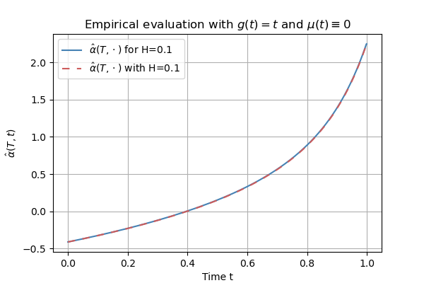
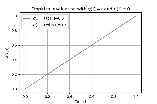
Figure 3: Approximation of $\alpha(T,\cdot)$ for different choices of $H$.

The variance shift observed in the RHS of Figure 5 for different choices of $H$ leads to a diversification in the variance of the perturbation kernels of GFDM observable in Figure 5 (top row). In order to have the same terminal variance for an arbitrary choice of $H\in(0,1)$ we normalize the function $\sigma$ for FVE to $\sigma(t)=\sigma_{max}\sqrt{\beta(t)}/\sigma_{T}$ and for FVP and sub-FVP to $\sqrt{\beta(t)\left(1-e^{-2\int^{2}_{0}\beta(s)ds}\right)}/\sigma_{T}$ such that we have the same terminal variance for all $H\in(0,1)$ since

$$\sigma^{2,VE}_{T}=\sigma^{2}_{max}\frac{c^{2}(T)\int_{0}^{T}\alpha^{2}(T,s)ds}{\sigma^{2}_{T}}=\sigma^{2}_{max}\quad\textit{and}\quad\sigma^{2,dyn}_{Tm}=\frac{c^{2}(T)\int_{0}^{T}\alpha^{2}(T,s)ds}{\sigma^{2}_{T}}=1$$ (110)

for $dyn\in\{FVP,subFVP\}$. The resulting variances over time are illustrated in fig. 4.

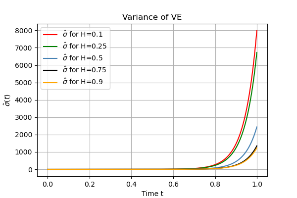
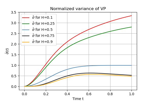
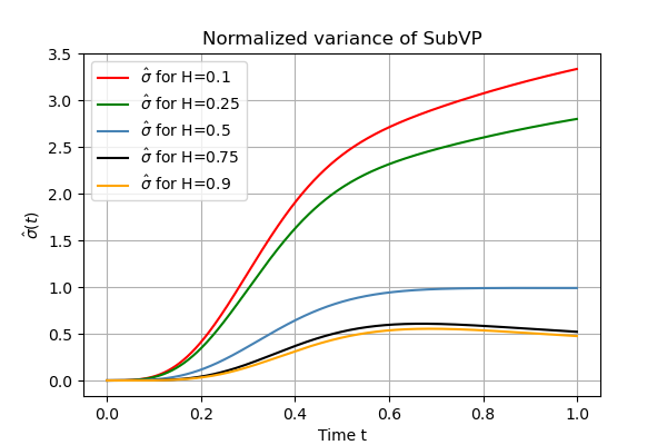
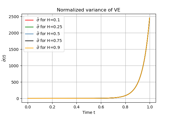
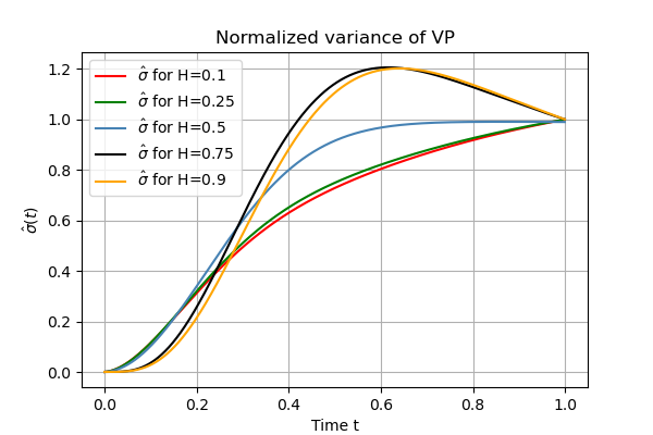
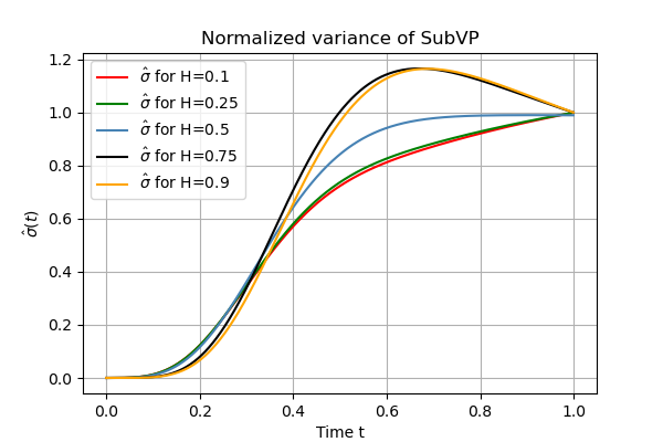
Figure 4: Top row: The variance shift of the underlying noise process for varying $H\in(0,1)$ leads to a diversification of the variance over time for FVE, FVP and sub-FVP. Bottom row: Variance normalization of the terminal variance leads to matching terminal variance across arbitrary choices of the Hurst index. Nevertheless, the resulting variance over time differs due to the variance differences of $W^{H,m}$ observable in the LHS of fig. 5.

To study the effect of varying Hurst index $H\in(0,1)$ on the covariance function of $\bm{X}$ we calculate for $X_{0}=0$, $d=1$ and $t_{1}<t_{2}\in[0,T]$

$$cov_{H}(X_{t_{1}},X_{t_{2}}) =\mathbb{E}\left[X_{t_{1}}X_{t_{2}}\right]-\mathbb{E}\left[X_{t_{1}}\right]\mathbb{E}\left[X_{t_{2}}\right]$$ (111)

$$=c(t_{1})c(t_{2})\mathbb{E}\left[\left(\int^{t_{1}}_{0}\alpha(t_{1},s)dW_{s}\right)\left(\int^{t_{2}}_{0}\alpha(t_{2},s)dW_{s}\right)\right]$$ (112)

and for $H=\frac{1}{2}$

$$cov(X_{t_{1}},X_{t_{2}}) =c(t_{1})c(t_{2})\mathbb{E}\left[\left(\int^{t_{1}}_{0}\alpha(s)dW_{s}\right)\left(\int^{t_{2}}_{0}\alpha(s)dW_{s}\right)\right]$$ (113)

$$=c(t_{1})c(t_{2})\left\{\int^{t_{1}}_{0}\alpha^{2}(s)ds+\mathbb{E}\left[\int^{t_{1}}_{0}\alpha(s)dW_{s}\int^{t_{2}}_{t_{1}}\alpha(s)dW_{s}\right]\right\}$$ (114)

$$=c(t_{1})c(t_{2})\left\{\int^{t_{1}}_{0}\alpha^{2}(s)ds\right\}$$ (115)

$$=\sigma^{2}_{t}\exp\left(-\int^{t_{2}}_{t_{1}}\mu(s)ds\right)$$ (116)

where we used Itôs symmetry and the independence of $W_{t_{1}}$ and $W_{t_{2}}-W_{t_{1}}$ resulting in

$$cov(X_{t_{1}}-X_{0},X_{t_{2}}-X_{1})=\sigma^{2}_{t}\left\{\exp\left(-\int^{t_{2}}_{t_{1}}\mu(s)ds\right)-1\right\}.$$ (117)

Hence for $FVE$ we find $cov(X_{t_{1}}-X_{0},X_{t_{2}}-X_{1})=0$ for $H=\frac{1}{2}$, while $cov(X_{t_{1}}-X_{0},X_{t_{2}}-X_{1})\not=0$ for $H\not=\frac{1}{2}$.

Appendix C Reverse Sampling

In accordance with Theorem 1 and the definition of $(\bm{Y}^{i},\bm{Z}^{i})$ in eq. 17 we initialize the reverse time model with

$$\bm{X}_{T}\sim\mathcal{N}\left(0,\sigma^{2}_{T}\bm{I}_{d}\right),\quad\bm{Y}^{i}_{T}\sim\mathcal{N}\left(0,\tau^{2}_{T,i}\bm{I}_{d}\right),\quad\bm{Z}^{i}_{T}\sim\mathcal{N}\left(0,\tilde{\tau}^{2}_{T,i}\bm{I}_{d}\right),$$ (118)

where

$$\tau^{2}_{T,i}=\frac{1}{2x_{i}}\left(1-e^{-2x_{i}T}\right),\quad\textit{and}\quad\tilde{\tau}^{2}_{T,i}=\frac{1}{4x^{3}_{i}}-\frac{(2T^{2}x^{2}+2Tx+1)e^{-2x_{i}T}}{4x^{3}_{i}}.$$ (119)

By Corollary 2 we sample for the initialization of the backward process only one random variable $\bm{\xi}\sim\mathcal{N}(\bm{0},\bm{I})$ to compute

$$\bm{X}_{T}=\sigma_{T}\bm{\xi},\quad\bm{Y}^{i}_{T}=\tau_{T,i}\bm{\xi},\quad Z^{i}_{T}=\tilde{\tau}_{T,i}\bm{\xi}$$ (120)

and

$$\bm{S}^{H}_{T}=\begin{cases}\sum_{i=1}^{m}q_{i}x_{i}\bm{Y}^{i}_{T},\quad&H\leq\frac{1}{2},\\ \sum_{i=1}^{m}q_{i}\left[x_{i}\bm{Z}^{i}_{T}-\bm{Y}^{i}_{T}\right],\quad&H>\frac{1}{2}.\end{cases}$$ (121)

We combine the Euler-Mayruyama solver (EMS) for SDEs and the Euler solver (ES) for ODEs to sample from the reverse time model. Denote by $SDE^{EMS}$ one step of the EMS and by $ODE^{ES}$ on step of the ES of the probability flow [Song et al., 2021] corresponding to the dynamics of the reverse time model derived in Theorem 3. In addition to SDE sampling using only EMS and ODE sampling using only ES we define two additional sampling methods by combining the two solvers to sample from the reverse time model. We define guided SDE generation (gSDE) by

$$\bm{X}_{t_{n}}=SDE^{EMS}\left(\bm{X}_{t_{n+1}}\right)\quad\textit{and}\quad\bm{Y}^{i}_{t_{n}}=ODE^{ES}\left(\bm{Y}^{i}_{t_{n+1}}\right)$$ (122)

and noisy ODE generation (nODE) by

$$\bm{X}_{t_{n}}=ODE^{ES}\left(\bm{X}_{t_{n+1}}\right)\quad\textit{and}\quad\bm{Y}^{i}_{t_{n}}=SDE^{EMS}\left(\bm{Y}^{i}_{t_{n+1}}\right).$$ (123)

Appendix D Space Grid Calculations

To calculate the space grid used in the definition of the process $W^{H,m}$ we first fix some even number $m\in\mathbb{N}$. Following the approximation scheme of Carmona et al. [2000] we fix $r\in(1,2)$ as well and define $\eta_{\frac{m}{2}-i}=r^{-i}$ for $-\frac{m}{2}\leq-i\leq 0$ and $\eta_{i+\frac{m}{2}}=r^{i}$ for $1\leq i\leq\frac{m}{2}$ such that $0<\eta_{0}<\eta_{1}<...<\eta_{m}$. Similar to equation (3.3) and (3.4) in Bäuerle and Desmettre [2020] we calculate for $H<\frac{1}{2}$

$$\int_{\eta^{m}_{i}}^{\eta^{m}_{i+1}}x\tilde{\nu}(dx)==\frac{\left[\left(\eta^{m}_{i+1}\right)^{\frac{3}{2}-H}-\left(\eta^{m}_{i}\right)^{\frac{3}{2}-H}\right]}{\left(\frac{3}{2}-H\right)\Gamma\left(H+\frac{1}{2}\right)\Gamma\left(\frac{1}{2}-H\right)}$$ (124)

and

$$\tilde{q}_{i+1}^{m}=\int_{\eta^{m}_{i}}^{\eta^{m}_{i+1}}\tilde{\nu}(dx)=\frac{\left[\left(\eta^{m}_{i+1}\right)^{\frac{1}{2}-H}-\left(\eta^{m}_{i}\right)^{\frac{1}{2}-H}\right]}{\left(\frac{1}{2}-H\right)\Gamma\left(H+\frac{1}{2}\right)\Gamma\left(\frac{1}{2}-H\right)}$$ (125)

resulting in

$$x^{m}_{i+1}=\frac{\int_{\eta^{m}_{i}}^{\eta^{m}_{i+1}}x\tilde{\nu}(dx)}{\int_{\eta^{m}_{i}}^{\eta^{m}_{i+1}}\tilde{\nu}(dx)}=\frac{(\frac{1}{2}-H)}{(\frac{3}{2}-H)}\left[\frac{\left(\eta^{m}_{i+1}\right)^{(\frac{3}{2}-H)}-\left(\eta^{m}_{i}\right)^{(\frac{3}{2}-H)}}{\left(\eta^{m}_{i+1}\right)^{(\frac{1}{2}-H)}-\left(\eta^{m}_{i}\right)^{(\frac{1}{2}-H)}}\right].$$ (126)

For $H>\frac{1}{2}$ we calculate

$$\int_{\eta^{m}_{i}}^{\eta^{m}_{i+1}}x\tilde{\nu}(dx)=\frac{\left[\left(\eta^{m}_{i+1}\right)^{\frac{5}{2}-H}-\left(\eta^{m}_{i}\right)^{\frac{3}{2}-H}\right]}{\left(\frac{5}{2}-H\right)\Gamma\left(H+\frac{1}{2}\right)\Gamma\left(\frac{5}{2}-H\right)}$$ (127)

and

$$\tilde{q}_{i+1}^{m}=\int_{\eta^{m}_{i}}^{\eta^{m}_{i+1}}\tilde{\nu}(dx)=\frac{\left[\left(\eta^{m}_{i+1}\right)^{\frac{3}{2}-H}-\left(\eta^{m}_{i}\right)^{\frac{3}{2}-H}\right]}{\left(\frac{3}{2}-H\right)\Gamma\left(H+\frac{1}{2}\right)\Gamma\left(\frac{3}{2}-H\right)}$$ (128)

such that

$$x^{m}_{i+1}=\frac{\int_{\eta^{m}_{i}}^{\eta^{m}_{i+1}}x\tilde{\nu}(dx)}{\int_{\eta^{m}_{i}}^{\eta^{m}_{i+1}}\tilde{\nu}(dx)}=\frac{(\frac{3}{2}-H)}{(\frac{5}{2}-H)}\left[\frac{\left(\eta^{m}_{i+1}\right)^{(\frac{5}{2}-H)}-\left(\eta^{m}_{i}\right)^{(\frac{5}{2}-H)}}{\left(\eta^{m}_{i+1}\right)^{(\frac{3}{2}-H)}-\left(\eta^{m}_{i}\right)^{(\frac{3}{2}-H)}}\right].$$ (129)

Using $\tilde{q}_{1},...,\tilde{q}_{m}$ in eq. 4 to define $\tilde{W}^{H,m}$ leads to a process with dynamics

$$d\tilde{W}^{H,m}_{t}=-g(t)S_{t}dt+c_{H}dW_{t},\quad\tilde{W}^{H,m}_{0}=0$$ (130)

and variance

$$\tilde{\sigma}^{2}_{m,r,t}=\begin{cases}\int^{t}_{0}\left(\sum_{i=1}^{m}\tilde{q}_{i}\left[e^{x_{i}(s-t)}\right]\right)^{2}ds,\quad&H<\frac{1}{2}\\ \int^{t}_{0}\left(\sum_{i=1}^{m}\tilde{q}_{i}(t-se^{x_{i}(s-t)})\right)^{2},\quad&H>\frac{1}{2}\end{cases}$$ (131)

where we used Theorem 1 to calculate $\tilde{\sigma}^{2}_{m,r,t}$. Using $m$ and $r$ as indices reflects that the variance of $\tilde{W}_{t}^{H,m}$ depends on $m$ and $r$. Since $\mathbb{V}[W^{H}_{1}]=1$, we aim to have $\mathbb{V}[\tilde{W}_{1}^{H,m}]=1$ as well for all choices of $H$, $m$ and $r$ but Figure 5 shows that we have $\tilde{\sigma}_{40,1.35,T}\not=1$ for the terminal variance . To ensure that $W^{H,m}$ provides a terminal variance of $\sigma^{2}_{m,r,T}=1$, we rescale $\tilde{q}_{1},...,\tilde{q}_{m}$ to

$$q_{i}=\frac{\tilde{q}_{i}}{a},\quad\textit{with}\quad a=\begin{cases}\left(\sum_{i=1}^{m}\tilde{q}_{i}e^{x_{i}(s-t)}\right)^{-\frac{1}{2}},\quad&H\leq\frac{1}{2}\\ \left(\sum_{i=1}^{m}\tilde{q}_{i}\left[(t-s)e^{x(s-t)}\right]\right)^{-\frac{1}{2}},\quad&H>\frac{1}{2}.\end{cases}$$ (132)

The Markovian representation from eq. 21 holds true for any rescaling of the measure by [Harms and Stefanovits, 2019, Remark 3.3] and hence in particular for $\nu=\tilde{\nu}/\tilde{c}$ and we use $q_{1},...,q_{m}$ and $\nu$ to define $W^{H,m}$ according to eq. 4.

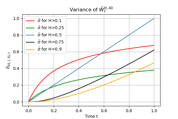
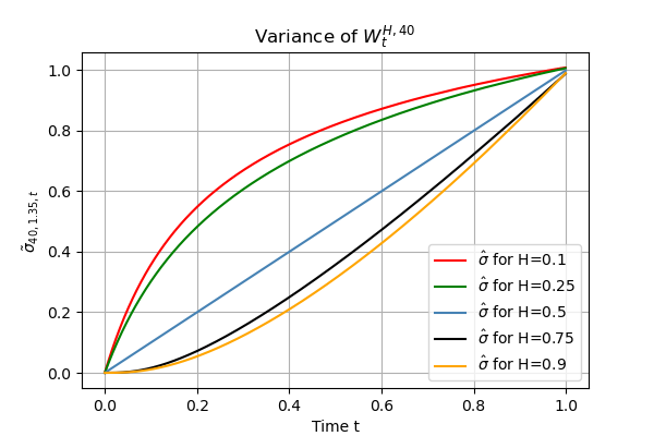
Figure 5: On the LHS the terminal variance of $\tilde{W}^{H,40}$ differs across choices of the Hurst indexx. Rescaling the measure $\nu=\tilde{\nu}/a$ results in alignment of the the terminal variances to $\sigma^{2}_{m,r,1}=1$ for any choice of the Hurst index.

Appendix E Experiments on Toy Data

	$H$	WSD $\downarrow$		IP $\uparrow$		IR $\uparrow$		VS $\uparrow$
		FVP	S.FVP	FVP	S.FVP	FVP	S.FVP	FVP	S.FVP
SDE	0.01	0.017	0.017	0.427	0.926	0.990	0.970	1.910	1.899
	0.25	0.014	0.013	0.510	0.929	0.995	0.971	1.910	1.899
	0.5	0.012	0.012	0.750	0.946	0.993	0.965	1.907	1.892
gSDE	0.01	0.034	0.029	0.418	0.961	0.989	0.964	1.950	1.946
	0.25	0.030	0.013	0.507	0.929	0.991	0.971	1.950	1.899
	0.5	-	-	-	-	-	-	-	-
nODE	0.01	0.056	0.050	0.936	0.989	0.966	0.912	1.963	1.951
	0.25	0.067	0.025	0.980	0.955	0.906	0.964	1.985	1.937
	0.5	0.011	0.011	0.913	0.947	0.976	0.968	1.903	1.906

Table 2: Quantitative results for the half moon dataset.

In Table 2 you find the quantitative results of GFDM on the half-moon dataset for the different sampling methods and varying $H\in\{0.5,0.25,0.1\}$. The high score in WSD reaches $H=0.5$, while the highest score in the other metrics is reached for $H<0.5$.

Appendix F Challenges in the Attempt to Generalize

In this work, we seek to determine the extent to which the continuous time framework of a score-based generative model can be generalized from an underlying BM to an FBM. For a FBM $W^{H}$ with Hurst index $H\in(0,1)$ it is not straightforward to define the the forward process

$$X_{T}=x_{0}+\int^{T}_{0}f(X_{t},t)dt+\int_{0}^{T}g(X_{t},t)dW^{H}_{t},\quad X_{0}\sim\mathcal{D},$$ (133)

driven by FBM, since FBM is neither a Markov process nor a semimartingale [Biagini et al., 2008], and hence Itô calculus may not be applied, to define the second integral. However, a definition of the integral w.r.t. FBM is established [Biagini et al., 2008, Hahn et al., 2011] as a discrete approximation of the integral w.r.t. FBM can rather simply be computed by the sum

$$\sum_{n=1}^{N}g(X_{t_{n}},t_{n})\Delta W^{H}_{n}\approx\int_{0}^{T}g(X_{t},t)dW^{H}_{t},$$

where $\Delta W^{H}_{1},...,\Delta W^{H}_{N}$ are the correlated and normally distributed increments of $W^{H}$. The more challenging difficulty in defining a generative model driven by FBM is to derive the reverse time model. Following the derivation of the reverse time model for BM, the conditional backward Kolmogorov equation and the unconditional forward Kolmogorov equation are applied [Anderson, 1982]. Starting point of the derivation is to rewrite $p(x_{t},t,x_{s},s)=p(x_{s},s|x_{t},t)p(x_{t},t)$ for $s\geq t$ using Bayes theorem to calculate with the product rule

$$\frac{\partial p(x_{t},t,x_{s},s)}{\partial t}=\frac{\partial p(x_{s},s|x_{t},t)}{\partial t}p(x_{t},t)+\frac{\partial p(x_{t},t)}{\partial t}p(x_{s},s|x_{t},t).$$ (134)

Replacing $\frac{\partial p(x_{t},t)}{\partial t}$ with the RHS of the unconditional forward Kolmogorov equation and $\frac{\partial p(x_{s},s|x_{t},t)}{\partial t}$ with the RHS of the conditional backward Kolmogorov equation one derives an equation that only depends on $p(x_{t},t,x_{s},s)$. Using Bayes theorem again leads to a conditional backward Kolmogorov equation for $p(x_{t},t|x_{s},s)$ that defines the dynamics of the reverse process by the one-to-one correspondence between the conditional backward Kolmogorov equation and the stochastic differential equation for the reverse process [Anderson, 1982]. Following these steps starting from eq. 134 and deploying a one-to-one correspondence of FBM and the evolution of its density [Hahn et al., 2011], we could replace $\frac{\partial p(x_{t},t)}{\partial t}$ in (134) by the RHS of

$$\frac{\partial p(x,t)}{\partial t}=\sum_{i=1}^{d}f_{i}(t,x)\frac{\partial p(t,x)}{\partial x_{i}}+Ht^{2H-1}\sum_{i,j=1}^{d}g_{ij}(x,t)\frac{\partial^{2}p(t,x)}{\partial x_{i}\partial x_{j}}$$ (135)

derived in Hahn et al. [2011]. The missing part is however analogous to the conditional backward Kolmogorov equation to replace $\frac{\partial p(x_{s},s|x_{t},t)}{\partial t}$ in eq. 134. The derivation of such an equation is a challenging and to the best of our knowledge yet unsolved problem. For that reason, we circumvent the need for a backward equation for the conditional density of FBM by following the approach in Harms and Stefanovits [2019] to represent the FBM in eq. 133 as a stochastic integral over a family of OU processes and approximate this integral in a second step as a weighted sum of OU processes. In this setting, we may apply Itô calculus and the conditional backward Kolmogorov equation to derive the reverse time model [Anderson, 1982].

References

- Anderson [1982] Brian D.O. Anderson. Reverse-time diffusion equation models. Stochastic Processes and their Applications, 12(3):313–326, 1982. ISSN 0304-4149. doi: https://doi.org/10.1016/0304-4149(82)90051-5. URL https://www.sciencedirect.com/science/article/pii/0304414982900515.
- Arjovsky et al. [2017] Martin Arjovsky, Soumith Chintala, and Léon Bottou. Wasserstein generative adversarial networks. In Doina Precup and Yee Whye Teh, editors, Proceedings of the 34th International Conference on Machine Learning, volume 70 of Proceedings of Machine Learning Research, pages 214–223. PMLR, 06–11 Aug 2017. URL https://proceedings.mlr.press/v70/arjovsky17a.html.
- Bäuerle and Desmettre [2020] Nicole Bäuerle and Sascha Desmettre. Portfolio optimization in fractional and rough heston models. SIAM Journal on Financial Mathematics, 11(1):240–273, 2020. doi: 10.1137/18M1217243. URL https://doi.org/10.1137/18M1217243.
- Biagini et al. [2008] Francesca Biagini, Yaozhong Hu, Bernt Øksendal, and Tusheng Zhang. Stochastic Calculus for Fractional Brownian Motion and Applications. Springer-Verlag London Limited 2008, 2008. doi: 10.1007/978-1-84628-797-8.
- Bunne et al. [2023] Charlotte Bunne, Ya-Ping Hsieh, Marco Cuturi, and Andreas Krause. The Schrödinger Bridge between Gaussian Measures has a closed form. In International Conference on Artificial Intelligence and Statistics (AISTATS), 2023.
- Carmona et al. [2000] Philippe Carmona, Laure Coutin, and G. Montseny. Approximation of some Gaussian Processes. Statistical Inference for Stochastic Processes, 3(1):161–171, 2000. doi: 10.1023/A:1009999518898.
- Chen et al. [2023] Sitan Chen, Sinho Chewi, Jerry Li, Yuanzhi Li, Adil Salim, and Anru R. Zhang. Sampling is as easy as learning the score: theory for diffusion models with minimal data assumptions. In The Eleventh International Conference on Learning Representations, 2023. URL https://openreview.net/forum?id=osei3IzUia.
- Cohen and J.Elliott [2015] Samuel N. Cohen and Robert J.Elliott. Stochastic Calculus and Applications. Probability and Its Applications. Birkhäuser, New York, NY, 2st edition, 2015. ISBN 978-1-4939-2866-8. doi: https://doi.org/10.1007/978-1-4939-2867-5.
- Friedman and Dieng [2022] Dan Friedman and Adji Bousso Dieng. The Vendi Score: A diversity evaluation metric for machine learning. arXiv preprint arXiv:2210.02410, 2022.
- Hahn et al. [2011] Marjorie G. Hahn, Kei Kobayashi, and Sabir Umarov. Fokker-Planck-Kolmogorov equations associated with time-changed fractional Brownian motion. arXiv: Mathematical Physics, 139:691–705, 2011.
- Harms [2019] Philipp Harms. Strong convergence rates for Markovian representations of fractional processes, 2019. URL https://arxiv.org/abs/1902.01471.
- Harms and Stefanovits [2019] Philipp Harms and David Stefanovits. Affine representations of fractional processes with applications in mathematical finance. Stochastic Processes and their Applications, 129(4):1185–1228, 2019. ISSN 0304-4149. doi: https://doi.org/10.1016/j.spa.2018.04.010. URL https://www.sciencedirect.com/science/article/pii/S0304414918301418.
- Ho et al. [2020] Jonathan Ho, Ajay Jain, and Pieter Abbeel. Denoising diffusion probabilistic models. In H. Larochelle, M. Ranzato, R. Hadsell, M.F. Balcan, and H. Lin, editors, Advances in Neural Information Processing Systems, volume 33, pages 6840–6851. Curran Associates, Inc., 2020.
- Huang et al. [2022] Chin-Wei Huang, Milad Aghajohari, Joey Bose, Prakash Panangaden, and Aaron C Courville. Riemannian diffusion models. In S. Koyejo, S. Mohamed, A. Agarwal, D. Belgrave, K. Cho, and A. Oh, editors, Advances in Neural Information Processing Systems, volume 35, pages 2750–2761. Curran Associates, Inc., 2022. URL https://proceedings.neurips.cc/paper_files/paper/2022/file/123d3e814e257e0781e5d328232ead9b-Paper-Conference.pdf.
- Itô [1987] Kiyosi Itô. Differential equations determining a markoff process. Kiyosi Itô: Selected Papers, Edit. DW Strook and SRS Varadhan, Springer, 1987.
- Jing et al. [2022] Bowen Jing, Gabriele Corso, Renato Berlinghieri, and Tommi Jaakkola. Subspace diffusion generative models. In Lecture Notes in Computer Science, pages 274–289. Springer Nature Switzerland, 2022. doi: 10.1007/978-3-031-20050-2_17. URL https://doi.org/10.1007%2F978-3-031-20050-2_17.
- Karras et al. [2022] Tero Karras, Miika Aittala, Timo Aila, and Samuli Laine. Elucidating the design space of diffusion-based generative models. In Proc. NeurIPS, 2022.
- Kynkäänniemi et al. [2019] Tuomas Kynkäänniemi, Tero Karras, Samuli Laine, Jaakko Lehtinen, and Timo Aila. Improved precision and recall metric for assessing generative models. CoRR, abs/1904.06991, 2019.
- Mandelbrot and Van Ness [1968] Benoit B. Mandelbrot and John W. Van Ness. Fractional brownian motions, fractional noises and applications. SIAM Review, 10(4):422–437, 1968. doi: 10.1137/1010093. URL https://doi.org/10.1137/1010093.
- Rogers [1997] L Chris G Rogers. Arbitrage with fractional brownian motion. Mathematical finance, 7(1):95–105, 1997.
- Singhal et al. [2023] Raghav Singhal, Mark Goldstein, and Rajesh Ranganath. Where to diffuse, how to diffuse, and how to get back: Automated learning for multivariate diffusions. In The Eleventh International Conference on Learning Representations, 2023. URL https://openreview.net/forum?id=osei3IzUia.
- Song and Ermon [2020] Yang Song and Stefano Ermon. Improved techniques for training score-based generative models. In H. Larochelle, M. Ranzato, R. Hadsell, M.F. Balcan, and H. Lin, editors, Advances in Neural Information Processing Systems, volume 33, pages 12438–12448. Curran Associates, Inc., 2020. URL https://proceedings.neurips.cc/paper_files/paper/2020/file/92c3b916311a5517d9290576e3ea37ad-Paper.pdf.
- Song et al. [2021] Yang Song, Jascha Sohl-Dickstein, Diederik P. Kingma, Abhishek Kumar, Stefano Ermon, and Ben Poole. Score-based generative modeling through stochastic differential equations. Preprint, February 2021. arXiv:2011.13456 [cs.LG].
- Song et al. [2023] Yang Song, Prafulla Dhariwal, Mark Chen, and Ilya Sutskever. Consistency models. arXiv preprint arXiv:2303.01469, 2023.