Positivity-preserving and entropy-bounded discontinuous Galerkin method for the chemically reacting, compressible Navier-Stokes equations

Abstract

This article concerns the development of a fully conservative, positivity-preserving, and entropy-bounded discontinuous Galerkin scheme for simulating the multicomponent, chemically reacting, compressible Navier-Stokes equations with complex thermodynamics. In particular, we extend to viscous flows the fully conservative, positivity-preserving, and entropy-bounded discontinuous Galerkin method for the chemically reacting Euler equations that we previously introduced. An important component of the formulation is the positivity-preserving Lax-Friedrichs-type viscous flux function devised by Zhang [J. Comput. Phys., 328 (2017), pp. 301-343], which was adapted to multicomponent flows by Du and Yang [J. Comput. Phys., 469 (2022), pp. 111548] in a manner that treats the inviscid and viscous fluxes as a single flux. Here, we similarly extend the aforementioned flux function to multicomponent flows but separate the inviscid and viscous fluxes, resulting in a different dissipation coefficient. This separation of the fluxes allows for use of other inviscid flux functions, as well as enforcement of entropy boundedness on only the convective contribution to the evolved state, as motivated by physical and mathematical principles. We also discuss in detail how to account for boundary conditions and incorporate previously developed pressure-equilibrium-preserving techniques into the positivity-preserving framework. Comparisons between the Lax-Friedrichs-type viscous flux function and more conventional flux functions are provided, the results of which motivate an adaptive solution procedure that employs the former only when the element-local solution average has negative species concentrations, nonpositive density, or nonpositive pressure. The resulting formulation is compatible with curved, multidimensional elements of arbitrary shape and general quadrature rules with positive weights. A variety of multicomponent, viscous flows is computed, ranging from a one-dimensional shock tube problem to multidimensional detonation waves and shock/mixing-layer interaction. We find that just as in the inviscid, multicomponent case, the robustness benefits of the enforcement of an entropy bound are much more pronounced than in the monocomponent, calorically perfect setting. Where appropriate, we demonstrate that mass, total energy, and atomic elements are discretely conserved.

1 Introduction

In the past two decades, interest in the discontinuous Galerkin (DG) method for fluid flow simulations has surged dramatically. This method benefits from arbitrarily high order of accuracy on unstructured grids, as well as a compact stencil and high arithmetic intensity suited for modern computing systems. However, one of the primary obstacles to widespread use of this numerical scheme is its susceptibility to nonlinear instabilities in underresolved regions and near non-smooth features. Robustness is an even greater concern when mixtures of thermally perfect gases and chemical reactions are considered [1, 2]. For instance, it is well-known that spurious pressure oscillations are generated in moving interface problems when fully conservative schemes are employed [3, 4, 5], often leading to solver divergence. A number of quasi-conservative methods, such as the double-flux technique [6, 7, 8], have been proposed to circumvent this issue, typically at the expense of energy conservation. Recently, two of the authors introduced a fully conservative DG scheme that does not generate such oscillations in smooth regions of the flow [2]. Strang splitting was employed to decouple the temporal integration of the convective and diffusive operators from that of stiff chemical source terms. Artificial viscosity was used to stabilize the solution near shocks and other non-smooth features. However, artificial viscosity alone is often not sufficient to guarantee stability. To further increase robustness, we made key advancements to this fully conservative DG method, focusing on the inviscid case, to ensure satisfaction of the positivity property (i.e., nonnegative species concentrations, positive density, and positive pressure) and an entropy bound based on the minimum entropy principle for the multicomponent Euler equations [9, 10], which states that the spatial minimum of specific thermodynamic entropy of entropy solutions is a nondecreasing function of time. The main ingredients of this DG formulation [10, 11] are (a) an invariant-region-preserving inviscid flux function [12], (b) a simple linear-scaling limiter [13], (c) satisfaction of a time-step-size constraint for the transport step with a strong-stability-preserving explicit time integrator, (d) incorporation of the pressure-equilibrium-preserving techniques introduced by Johnson and Kercher [2], and (e) an entropy-stable DG discretization in time based on diagonal-norm summation-by-parts operators for the reaction step. It was found that the formulation was capable of robustly and accurately computing complex inviscid, reacting flows using high-order polynomials and relatively coarse meshes. Enforcement of entropy boundedness was critical for stability in simulations of multidimensional detonation waves.

The consideration of viscous flows brings about additional complications. Using conventional viscous flux functions, such as the second form of Bassi and Rebay (BR2) [14] and the symmetric interior penalty method (SIPG) [15], positivity is not guaranteed to be maintained. Specifically, it is possible for the constraint on the time step size to be arbitrarily small for the solution to satisfy said property. To remedy this problem, Zhang [16] introduced a Lax-Friedrichs-type viscous flux function for the monocomponent Navier-Stokes equations, accompanied by a strictly positive upper bound on the time step size to guarantee satisfaction of the positivity property. Although it may be surprising that the viscous flux can be a primary source of negative concentrations, nonpositive density, and/or nonpositive pressure, we call attention to certain numerical challenges specific to multicomponent-flow simulations: not only are nonlinear instabilities more likely to occur, but also species concentrations are typically close or equal to zero, such that small numerical errors can easily lead to negative concentrations. Furthermore, in the monocomponent case, the mass conservation equation is identical between the Euler system and the Navier-Stokes system; therefore, the diffusive operator does not directly contribute to negative densities. However, this is not true in the multicomponent case, which means that the viscous flux can indeed be largely responsible for negative concentrations. Note that many multicomponent-flow codes simply “clip” negative species concentrations, but such an intrusive strategy violates mass conservation and pollutes the solution with low-order errors.

Du and Yang [17] recently extended the aforementioned Lax-Friedrichs-type viscous flux function to multicomponent flows. Specifically, they combined the inviscid and viscous fluxes into a single flux, such that the resulting dissipation coefficient accounts for both fluxes simultaneously. Entropy boundedness was not considered. Instead of operator splitting, they employed an exponential multistage/multistep, explicit time integration scheme [18, 19, 20] that can handle stiff source terms. Although in the present study we use operator splitting since it has proven successful to date and its accuracy is less reliant on “well-prepared” initial conditions [18, 19, 20], exponential multistage/multistep time integrators are indeed worthy of future investigation.

In this work, we develop a fully conservative, positivity-preserving, and entropy-bounded DG method for the compressible, multicomponent, chemically reacting Navier-Stokes equations. We focus on the transport step since the treatment of stiff chemical source terms is identical to that in the inviscid case. Enforcement of a lower bound on the specific thermodynamic entropy is performed on only the convective contribution to the evolved state since the viscous flux function is not fully compatible with said entropy bound. This was also done by Dzanic and Witherden [21], albeit in a different manner, in their entropy-based filtering framework. Furthermore, at least in the monocomponent, calorically perfect setting, the minimum entropy principle does not hold for the Navier-Stokes equations unless the thermal diffusivity is zero [22, 23]. Although such analysis has not yet been performed for the multicomponent Navier-Stokes equations with the thermally perfect gas model, we do not expect the conclusion to change. Our primary contributions are as follows:

• We extend the aforementioned positivity-preserving Lax-Friedrichs-type viscous flux function [16] to multicomponent flows. Specifically, unlike in [17], we treat the inviscid and viscous fluxes separately, resulting in a different dissipation coefficient. The rationale for separating the fluxes is twofold. First, enforcing a bounded entropy on the convective contribution necessitates isolating the fluxes. Secondly, in our experience, we have found the HLLC inviscid flux function to perform more favorably than the Lax-Friedrichs inviscid flux function. We also discuss the treatment of boundary conditions in more detail.

• Entropy boundedness is enforced on only the convective contribution in a rigorous manner that maintains full compatibility with the positivity property.

• We show that if any of the species concentrations is zero, then the Lax-Friedrichs-type viscous flux function alone cannot guarantee that all species concentrations (or more specifically, their element averages) at the following time step remain nonnegative. This is true regardless of whether the inviscid and viscous fluxes are treated simultaneously or separately. A remedy for this pathological case is proposed.

• We incorporate the pressure-equilibrium-preserving techniques by Johnson and Kercher [2] into the positivity-preserving framework, which imposes an additional constraint on the time step size.

• The performance of the Lax-Friedrichs-type viscous flux function is assessed. Optimal convergence for smooth flows is observed. However, comparisons with the BR2 scheme indicate that when possible, the latter is generally still preferred. As such, we employ an adaptive solution procedure that only employs the Lax-Friedrichs-type viscous flux function when necessary.

• The proposed formulation is compatible with multidimensional elements of arbitrary shape and geometric-approximation order. We first apply it to a series of one-dimensional viscous flows: advection-diffusion of a thermal bubble, a premixed flame, and shock-tube flow. More complex viscous flow problems are then considered, namely a two-dimensional detonation wave enclosed by adiabatic walls and three-dimensional shock/mixing-layer interaction. Discrete conservation of mass, total energy, and atomic elements is demonstrated. Just as in the inviscid case, enforcement of the entropy bound significantly improves the stability of the solution.

The remainder of this article is organized as follows. The governing equations, transport properties, and thermodynamic relations are summarized in Section 2, followed by a review of the basic DG discretization in Section 3. Section 4 presents the positivity-preserving and entropy-bounded DG method for the transport step. Results for a variety of test cases are given in the next section. The paper concludes with some final remarks.

2 Governing equations

The compressible, multicomponent, chemically reacting Navier-Stokes equations in $d$ spatial dimensions are given by

$$\frac{\partial y}{\partial t}+\nabla\cdot\mathcal{F}\left(y,\nabla y\right)-\mathcal{S}\left(y\right)=0,$$ (2.1)

where $y$ is the state vector, $\nabla y$ is its spatial gradient, $t$ is time, $\mathcal{F}$ is the flux, and $\mathcal{S}=\left(0,\ldots,0,0,\omega_{1},\ldots,\omega_{n_{s}}\right)^{T}$ is the chemical source term, with $\omega_{i}$ corresponding to the production rate of the $i$th species. The physical coordinates are denoted by $x=(x_{1},\ldots,x_{d})$. The vector of state variables is expanded as

$$y=\left(\rho v_{1},\ldots,\rho v_{d},\rho e_{t},C_{1},\ldots,C_{n_{s}}\right)^{T},$$ (2.2)

where $\rho$ is density, $v=\left(v_{1},\ldots,v_{d}\right)$ is the velocity vector, $e_{t}$ is the specific total energy, $C=\left(C_{1},\ldots,C_{n_{s}}\right)$ is the vector of molar concentrations, and $n_{s}$ is the number of species. The partial density of the $i$th species is defined as

$$\rho_{i}=W_{i}C_{i},$$

where $W_{i}$ is the molecular weight of the $i$th species, from which the density can be computed as

$$\rho=\sum_{i=1}^{n_{s}}\rho_{i}.$$

The mole and mass fractions of the $i$th species are given by

$$X_{i}=\frac{C_{i}}{\sum_{i=1}^{n_{s}}C_{i}},\quad Y_{i}=\frac{\rho_{i}}{\rho}.$$

The equation of state for the mixture is written as

$$P=R^{0}T\sum_{i=1}^{n_{s}}C_{i},$$ (2.3)

where $P$ is the pressure, $T$ is the temperature, and $R^{0}$ is the universal gas constant. The specific total energy is the sum of the mixture-averaged specific internal energy, $u$, and the specific kinetic energy, written as

$$e_{t}=u+\frac{1}{2}\sum_{k=1}^{d}v_{k}v_{k},$$

where the former is the mass-weighted sum of the specific internal energies of each species, given by

$$u=\sum_{i=1}^{n_{s}}Y_{i}u_{i}.$$

With the thermally perfect gas model, $u_{i}$ is defined as

$$u_{i}=h_{i}-R_{i}T=h_{\mathrm{ref},i}+\int_{T_{\mathrm{ref}}}^{T}c_{p,i}(\tau)d\tau-R_{i}T,$$

where $h_{i}$ is the specific enthalpy of the $i$th species, $R_{i}=R^{0}/W_{i}$, $T_{\mathrm{ref}}$ is the reference temperature of 298.15 K, $h_{\mathrm{ref},i}$ is the reference-state species formation enthalpy, and $c_{p,i}$ is the specific heat at constant pressure of the $i$th species, which is approximated with a polynomial as a function of temperature based on the NASA coefficients [24, 25], i.e.,

$$c_{p,i}=\sum_{k=0}^{n_{p}}a_{ik}T^{k}.$$ (2.4)

The mixture-averaged specific thermodynamic entropy is obtained via a mass-weighted sum of the specific entropies of each species as

$$s=\sum_{i=1}^{n_{s}}Y_{i}s_{i},$$

with $s_{i}$ defined as

$$s_{i}=s_{\mathrm{ref},i}^{o}+\int_{T_{\mathrm{ref}}}^{T}\frac{c_{v,i}(\tau)}{\tau}d\tau-R_{i}\log\frac{C_{i}}{C_{\mathrm{ref}}},$$

where $s_{\mathrm{ref},i}^{o}$ is the species formation entropy at the reference temperature and reference pressure, $P_{\mathrm{ref}}$, of 1 atm, $c_{v,i}=c_{p,i}-R_{i}$ is the specific heat at constant volume of the $i$th species, and $C_{\mathrm{ref}}=P_{\mathrm{ref}}/R^{0}T_{\mathrm{ref}}$ is the reference concentration.

The flux can be expressed as the difference between the convective flux, $\mathcal{F}^{c}$, and the viscous flux, $\mathcal{F}^{v}$, i.e.,

$$\mathcal{F}\left(y,\nabla y\right)=\left(\mathcal{F}^{c}\left(y\right)-\mathcal{F}^{v}\left(y,\nabla y\right)\right),$$

where the $k$th spatial components are defined as

$$\mathcal{F}_{k}^{c}\left(y\right)=\left(\rho v_{k}v_{1}+P\delta_{k1},\ldots,\rho v_{k}v_{d}+P\delta_{kd},v_{k}\left(\rho e_{t}+P\right),v_{k}C_{1},\ldots,v_{k}C_{n_{s}}\right)^{T}$$ (2.5)

and

$$\mathcal{F}_{k}^{v}\left(y,\nabla y\right)=\left(\tau_{1k},\ldots,\tau_{dk},\sum_{j=1}^{d}\tau_{kj}v_{j}+\sum_{i=1}^{n_{s}}W_{i}C_{i}h_{i}V_{ik}-q_{k},C_{1}V_{1k},\ldots,C_{n_{s}}V_{n_{s}k}\right)^{T},$$ (2.6)

respectively. $\tau$ is the viscous stress tensor, $q$ is the heat flux, and $V_{ik}$ is the $k$th spatial component of the diffusion velocity of the $i$th species, defined as

$$V_{ik}=\hat{V}_{ik}-\frac{\sum_{l=1}^{n_{s}}W_{l}C_{l}\hat{V}_{lk}}{\rho},\quad\hat{V}_{ik}=\frac{\bar{D}_{i}}{C_{i}}\frac{\partial C_{i}}{\partial x_{k}}-\frac{\bar{D}_{i}}{\rho}\frac{\partial\rho}{\partial x_{k}},$$

which includes a standard correction to ensure mass conservation (i.e., $\sum_{i=1}^{n_{s}}W_{i}C_{i}V_{ik}=0$) [26, 27]. $\bar{D}_{i}$ is the mixture-averaged diffusion coefficient of the $i$th species, obtained as [28]

$$\bar{D}_{i}=\frac{1}{\bar{W}}\frac{\sum_{j=1,j\neq i}^{n_{s}}X_{j}W_{j}}{\sum_{j=1,j\neq i}^{n_{s}}X_{j}/D_{ij}},$$

where $\bar{W}=\rho/\sum_{i}C_{i}$ is the mixture molecular weight and $D_{ij}$ is the binary diffusion coefficient between the $i$th and $j$th species, which is a positive function of temperature and pressure [29, 30]. Note that $\bar{D}_{i}$ can be nonzero for $C_{i}=0$. The $k$th spatial components of the viscous stress tensor and the heat flux are written as

$$\tau_{k}\left(y,\nabla y\right)=\mu\left(\frac{\partial v_{1}}{\partial x_{k}}+\frac{\partial v_{k}}{\partial x_{1}}-\delta_{k1}\frac{2}{3}\sum_{j=1}^{d}\frac{\partial v_{j}}{\partial x_{j}},\ldots,\frac{\partial v_{d}}{\partial x_{k}}+\frac{\partial v_{k}}{\partial x_{d}}-\delta_{kd}\frac{2}{3}\sum_{j=1}^{d}\frac{\partial v_{j}}{\partial x_{j}}\right),$$

where $\mu$ is the dynamic viscosity, calculated using the Wilke model [31], and

$$q_{k}\left(y,\nabla y\right) = -\lambda_{T}\frac{\partial T}{\partial x_{k}},$$

where $\lambda_{T}$ is the thermal conductivity, computed with the Mathur model [32], respectively. The viscous flux can also be written as

$$\mathcal{F}^{v}\left(y,\nabla y\right)=G\left(y\right):\nabla y$$ (2.7)

where $G\left(y\right)$ is the homogeneity tensor [33], obtained by differentiating the viscous flux with respect to the gradient, i.e., $G(y)=\partial\mathcal{F}^{v}/\partial\nabla y$. Additional information on the thermodynamic relations, transport properties, and chemical reaction rates can be found in [2] and [10].

3 Discontinuous Galerkin discretization

This section summarizes the DG discretization of Equation 2.1 and the approach introduced by Johnson and Kercher [2] to suppress spurious pressure oscillations in smooth regions of the flow.

Let the computational domain, $\Omega$, be partitioned by $\mathcal{T}$, which consists of non-overlapping cells, $\kappa$, with boundaries $\partial\kappa$. Let $\mathcal{E}=\mathcal{E_{I}}\cup\mathcal{E}_{\partial}$ be the set of interfaces, $\epsilon$, such that $\cup_{\epsilon\in\mathcal{E}}\epsilon=\cup_{\kappa\in\mathcal{T}}\partial\kappa$, comprised of the interior interfaces,

$$\epsilon_{\mathcal{I}}\in\mathcal{E_{I}}=\left\{\epsilon_{\mathcal{I}}\in\mathcal{E}\,\middle|\,\epsilon_{\mathcal{I}}\cap\partial\Omega=\emptyset\right\},$$

and boundary interfaces,

$$\epsilon_{\partial}\in\mathcal{E}_{\partial}=\left\{\epsilon_{\partial}\in\mathcal{E}\,\middle|\,\epsilon_{\partial}\subset\partial\Omega\right\}.$$

At a given interior interface, there exists $\kappa^{+},\kappa^{-}\in\mathcal{T}$ such that $\epsilon_{\mathcal{I}}=\partial\kappa^{+}\cap\partial\kappa^{-}$. $n^{+}$ is the outward-facing normal of $\kappa^{+}$, and $n^{+}=-n^{-}$. The discrete subspace $V_{h}^{p}$ over $\mathcal{T}$ is defined as

$$V_{h}^{p} = \left\{\mathfrak{v}\in\left[L^{2}\left(\Omega\right)\right]^{m}\,\middle|\,\forall\kappa\in\mathcal{T},\left.\mathfrak{v}\right|_{\kappa}\in\left[\mathcal{P}_{p}(\kappa)\right]^{m}\right\},$$ (3.1)

where $m=n_{s}+d+1$ is the number of state variables and $\mathcal{P}_{p}(\kappa)$ in one spatial dimension is the space of polynomial functions of degree no greater than $p$ in $\kappa$. In multiple dimensions, the choice of polynomial space often depends on the element type [33].

To solve for the discrete solution, we require $y\in V_{h}^{p}$ to satisfy

$$\sum_{\kappa\in\mathcal{T}}\left(\frac{\partial y}{\partial t},\mathfrak{v}\right)_{\kappa}-\sum_{\kappa\in\mathcal{T}}\left(\mathcal{F}^{c}\left(y,\nabla y\right),\nabla\mathfrak{v}\right)_{\kappa}+\sum_{\epsilon\in\mathcal{E}}\left(\mathcal{F}^{c\dagger}\left(y,n\right),\left\llbracket\mathfrak{v}\right\rrbracket\right)_{\epsilon}-\sum_{\epsilon\in\mathcal{E}}\left(\left\{\!\!\left\{\mathcal{F}^{v}\left(y,\nabla y\right)\right\}\!\!\right\}\cdot n-\delta^{v}\left(y,\nabla y,n\right),\left\llbracket\mathfrak{v}\right\rrbracket\right)_{\epsilon}$$

$$+\sum_{\kappa\in\mathcal{T}}\left(G\left(y^{+}\right):\left(\left\{\!\!\left\{y\right\}\!\!\right\}-y^{+}\right)\otimes n,\nabla\mathfrak{v}\right)_{\partial\kappa}-\sum_{\kappa\in\mathcal{T}}\left(\mathcal{S}\left(y\right),\mathfrak{v}\right)_{\kappa}=0\qquad\forall\mathfrak{v}\in V_{h}^{p},$$ (3.2)

where $\left(\cdot,\cdot\right)$ denotes the inner product, $\mathcal{F}^{c\dagger}$ is the inviscid flux function, $\left\{\!\!\left\{\cdot\right\}\!\!\right\}$ is the average operator, $\left\llbracket\cdot\right\rrbracket$ is the jump operator, and $\delta^{v}$ is a viscous-flux penalty term that depends on the viscous flux function. Note that Equation (3.2) corresponds to a primal formulation [34, 33]; in [16], a flux formulation is used. It is worth mentioning that the penalty term for many conventional viscous flux functions is not a function of the gradient, i.e., $\delta^{v}=\delta^{v}(y,n)$; however, as will be seen in Section 4.1, the penalty term for the proposed Lax-Friedrichs-type viscous flux function indeed depends on the gradient. In this work, we employ the HLLC inviscid numerical flux [35]. To compute $\delta^{v}$, we consider the BR2 scheme [14] and the proposed Lax-Friedrichs-type flux function. The jump operator, average operator, inviscid flux function, and penalty term are defined as

$$\left\llbracket v\right\rrbracket=v^{+}-v^{-} \textup{ on }\epsilon\qquad\forall\epsilon\in\mathcal{E_{I}},$$

$$\left\{\!\!\left\{y\right\}\!\!\right\}=\frac{1}{2}\left(y^{+}+y^{-}\right) \textup{ on }\epsilon\qquad\forall\epsilon\in\mathcal{E_{I}},$$

$$\left\{\!\!\left\{\mathcal{F}^{\nu}\left(y,\nabla y\right)\right\}\!\!\right\}=\frac{1}{2}\left(\mathcal{F}^{\nu}\left(y^{+},\nabla y^{+}\right)+\mathcal{F}^{\nu}\left(y^{-},\nabla y^{-}\right)\right) \textup{ on }\epsilon\qquad\forall\epsilon\in\mathcal{E_{I}},$$

$$\mathcal{F}^{c\dagger}\left(y,n\right)=\mathcal{F}^{c\dagger}\left(y^{+},y^{-},n\right) \textup{ on }\epsilon\qquad\forall\epsilon\in\mathcal{E_{I}},$$

$$\delta^{v}\left(y,\nabla y,n\right)=\delta^{v}\left(y^{+},y^{-},\nabla y^{+},\nabla y^{-},n\right) \textup{ on }\epsilon\qquad\forall\epsilon\in\mathcal{E_{I}},$$

at interior interfaces and

$$\left\llbracket v\right\rrbracket=v^{+} \textup{ on }\epsilon\qquad\forall\epsilon\in\mathcal{E}_{\partial},$$

$$\left\{\!\!\left\{y\right\}\!\!\right\}=y_{\partial}\left(y^{+},n^{+}\right) \textup{ on }\epsilon\qquad\forall\epsilon\in\mathcal{E}_{\partial},$$

$$\left\{\!\!\left\{\mathcal{F}^{\nu}\left(y,\nabla y\right)\right\}\!\!\right\}=\mathcal{F}_{\partial}^{\nu}\left(y_{\partial}\left(y^{+},n^{+}\right),\nabla y^{+}\right) \textup{ on }\epsilon\qquad\forall\epsilon\in\mathcal{E}_{\partial},$$

$$\mathcal{F}^{c\dagger}\left(y,n\right)=\mathcal{F}_{\partial}^{c\dagger}\left(y^{+},n^{+}\right) \textup{ on }\epsilon\qquad\forall\epsilon\in\mathcal{E}_{\partial},$$

$$\delta^{v}\left(y,\nabla y,n\right)=\delta_{\partial}^{v}\left(y^{+},y_{\partial}\left(y^{+},n^{+}\right),\nabla y^{+},n^{+}\right) \textup{ on }\epsilon\qquad\forall\epsilon\in\mathcal{E}_{\partial},$$

at boundary interfaces, where $y_{\partial}\left(y^{+},n^{+}\right)$ is the boundary state, $\mathcal{F}_{\partial}^{c\dagger}\left(y^{+},n^{+}\right)$ is the inviscid boundary flux function, $\mathcal{F}_{\partial}^{\nu}\left(y_{\partial}\left(y^{+}\right),\nabla y^{+},n^{+}\right)$ is the viscous boundary flux, and $\delta_{\partial}^{v}\left(y^{+},y_{\partial}\left(y^{+},n^{+}\right),\nabla y^{+},n^{+}\right)$ is the boundary penalty term. A provides a discussion of the prescription of various boundary conditions.

Strang splitting [36] is applied to decouple the temporal integration of the transport operators from that of the stiff chemical source term over a given interval $(t_{0},t_{0}+\Delta t]$ as

$$\frac{\partial y}{\partial t}+\nabla\cdot\mathcal{F}\left(y\right)=0 \textup{ in }\Omega\times\left(t_{0},t_{0}+\nicefrac{{\Delta t}}{{2}}\right],$$ (3.3)

$$\frac{\partial y}{\partial t}-\mathcal{S}\left(y\right)=0 \textup{ in }\left(t_{0},t_{0}+\Delta t\right],$$ (3.4)

$$\frac{\partial y}{\partial t}+\nabla\cdot\mathcal{F}\left(y\right)=0 \textup{ in }\Omega\times\left(t_{0}+\nicefrac{{\Delta t}}{{2}},t_{0}+\Delta t\right].$$ (3.5)

Equations (3.3) and (3.5) are advanced in time using a strong-stability-preserving Runge-Kutta method (SSPRK) [37, 38], whereas Equation (3.4) is solved using a fully implicit, temporal DG discretization. Since the reaction step is identical between the inviscid and viscous cases, we refer the reader to [10] and [11] for more details on the DG discretization in time for Equation (3.4). Here, we focus on the transport step.

We assume a nodal basis, such that the local solution approximation is given by

$$y_{\kappa}=\sum_{j=1}^{n_{b}}y_{\kappa}(x_{j})\phi_{j},$$ (3.6)

where $\phi_{j}$ is the $j$th basis function, $n_{b}$ is the number of basis functions, and $x_{j}$ is the physical coordinate of the $j$th node. Unless otherwise specified, the volume and surface integrals in Equation (3.2) are computed using a quadrature-free approach [39, 40]. Furthermore, the flux can be approximated as

$$\mathcal{F_{\kappa}}\left(y\right)\approx\sum_{k=1}^{n_{c}}\mathcal{F}\left(y_{\kappa}\left(x_{k}\right),\nabla y_{\kappa}\left(x_{k}\right)\right)\varphi_{k},$$ (3.7)

where $n_{c}\geq n_{b}$ and $\left\{\varphi_{1},\ldots,\varphi_{n_{c}}\right\}$ is a set of basis functions that may be different from those in Equation (3.6). As discussed in [2], pressure equilibrium is maintained in smooth regions of the flow and at material interfaces if $n_{c}=n_{b}$ and the integration points are in the solution nodal set. However, if over-integration is desired (i.e., $n_{c}>n_{b}$), the standard flux interpolation (3.7) results in the generation of spurious pressure oscillations. Therefore, in the case of over-integration, Equation (3.7) is replaced with

$$\mathcal{F_{\kappa}}\left(y\right)\approx\sum_{k=1}^{n_{c}}\mathcal{F}_{\kappa}\left(\widetilde{y}_{\kappa}\left(x_{k}\right),\nabla y_{\kappa}\left(x_{k}\right)\right)\varphi_{k}=\sum_{k=1}^{n_{c}}\mathcal{F}_{\kappa}^{c}\left(\widetilde{y}_{\kappa}\left(x_{k}\right)\right)\varphi_{k}-\sum_{k=1}^{n_{c}}\mathcal{F}_{\kappa}^{v}\left(\widetilde{y}_{\kappa}\left(x_{k}\right),\nabla y_{\kappa}\left(x_{k}\right)\right)\varphi_{k},$$ (3.8)

where

$$\mathcal{F}_{\kappa}^{v}\left(\widetilde{y}_{\kappa}\left(x_{k}\right),\nabla y_{\kappa}\left(x_{k}\right)\right)=G\left(\widetilde{y}_{\kappa}\left(x_{k}\right)\right):\nabla y_{\kappa}\left(x_{k}\right)$$

and $\widetilde{y}$ is a modified state given by

$$\widetilde{y}\left(y,\widetilde{P}\right)=\left(\rho v_{1},\ldots,\rho v_{d},\widetilde{\rho u}\left(C_{1},\ldots,C_{n_{s}},\widetilde{P}\right)+\frac{1}{2}\sum_{k=1}^{d}\rho v_{k}v_{k},C_{1},\ldots,C_{n_{s}}\right)^{T}.$$ (3.9)

$\widetilde{P}$ in Equation (3.9) is a polynomial in $\mathcal{P}_{p}(\kappa)$ that approximates the pressure as

$$\widetilde{P}_{\kappa}=\sum_{j=1}^{n_{b}}P\left(y_{\kappa}\left(x_{j}\right)\right)\phi_{j},$$

from which the modified internal energy, $\widetilde{\rho u}$, is calculated. Furthermore, in Equation (3.2), $\delta^{v}\left(y,\nabla y,n\right)$ and $G\left(y^{+}\right):\left(\left\{\!\!\left\{y\right\}\!\!\right\}-y^{+}\right)\otimes n$ are replaced with $\delta^{v}\left(\widetilde{y},\nabla y,n\right)$ and $G\left(\widetilde{y}^{+}\right):\left(\left\{\!\!\left\{\widetilde{y}\right\}\!\!\right\}-\widetilde{y}^{+}\right)\otimes n$, respectively. The modified flux interpolation (3.8) successfully preserves pressure equilibrium within and between elements (unless the solution is not adequately resolved, in which case measurable pressure disturbances are inevitable).

Since the linear-scaling limiter used to enforce the positivity property and entropy boundedness does not completely eliminate small-scale nonphysical artifacts [13, 12, 41, 42], especially near non-smooth features, we add the artificial dissipation term [33]

$$-\sum_{\kappa\in\mathcal{T}}\left(\nu_{\mathrm{AV}}\nabla y,\nabla\mathfrak{v}\right)_{\kappa}$$ (3.10)

to the LHS of Equation (3.2), where $\nu_{\mathrm{AV}}$ is the artificial viscosity, calculated as [2]

$$\nu_{\mathrm{AV}}=\left(C_{\mathrm{AV}}+S_{\mathrm{AV}}\right)\left(\frac{h^{2}}{p+1}\left|\frac{\partial T}{\partial y}\cdot\frac{\mathcal{R}\left(y,\nabla y\right)}{T}\right|\right).$$

$S_{\mathrm{AV}}$ is a shock sensor based on solution variations inside a given element [43], $C_{\mathrm{AV}}$ is a user-defined parameter, $h$ is a length scale associated with the element, and $\mathcal{R}\left(y,\nabla y\right)$ is the strong form of the residual (2.1). In our previous work, this artificial viscosity formulation effectively mitigated small-scale nonlinear instabilities in various multicomponent-flow problems [2, 10]. However, other types of artificial viscosity or limiters can be employed instead. Additional details on the basic DG discretization and the issue of pressure equilibrium preservation can be found in [2].

4 Transport step: Positivity-preserving, entropy-bounded discontinuous Galerkin method

Let $\mathcal{G}_{\sigma}$ denote the following set:

$$\mathcal{G}_{\sigma}=\left\{y\mid\rho>0,\rho u^{*}>0,C_{1}\geq 0,\ldots,C_{n_{s}}\geq 0,\chi_{\sigma}\geq 0\right\},$$ (4.1)

where $\sigma\in\mathbb{R}$, $\chi_{\sigma}=\rho s-\rho\sigma$, and $u^{*}$ is the “shifted” internal energy [44], calculated as

$$u^{*}=u-u_{0},\quad u_{0}=\left.u\right|_{T=0},$$ (4.2)

such that $u^{*}>0$ if and only if $T>0$, provided $c_{v,i}>0,\>i=1,\ldots,n_{s}$ [45]. Note that $\rho>0$ and $u^{*}>0$ imply $P(y)>0$. The $\chi_{\sigma}>0$ inequality is associated with entropy boundedness, which will be discussed in more detail later in this section. Let $\mathcal{G}$ denote a similar set, but without the entropy constraint, i.e.,

$$\mathcal{G}=\left\{y\mid\rho>0,\rho u^{*}>0,C_{1}\geq 0,\ldots,C_{n_{s}}\geq 0\right\}.$$ (4.3)

Since $\rho u^{*}(y)$ is a concave function of the state [10], $\mathcal{G}$ is a convex set. If all species concentrations are strictly positive, then for a given $\sigma$, $\chi_{\sigma}$ is concave [12, 10, 9] and $\mathcal{G}_{\sigma}$ is also a convex set. However, if any of the species concentrations is zero, then $\chi_{\sigma}$ is no longer concave [9, 46]. For the remainder of this paper, in any discussion of entropy, $\mathcal{G}_{\sigma}$ is always assumed to be a convex set. Note that this assumption does not seem to have any discernible negative effects on the solver [10, 11]. In addition, as will be made clear in the upcoming subsection and Remark 2, positive species concentrations are assumed until Section 4.7, wherein this restriction is relaxed to allow for consideration of zero concentrations.

4.1 Positivity-preserving Lax-Friedrichs-type viscous flux function

In this subsection, we extend the local Lax-Friedrichs-type viscous flux function by Zhang [16] to multicomponent flows with species diffusion. In particular, we consider the viscous flux separately from the inviscid flux, unlike Du and Yang [17], who adapted said flux function to multicomponent flows in a manner that treats both fluxes simultaneously. Unless otherwise specified, we assume this flux function is employed for the remainder of the section. The penalty term takes the form [16]

$$\delta^{v}(y^{+},y^{-},\nabla y^{+},\nabla y^{-},n)=\frac{\beta}{2}\left(y^{+}-y^{-}\right),$$

where $\beta>0$ is the dissipation coefficient. The lemma below introduces a constraint on the definition of $\beta$ that is essential for satisfaction of the positivity property by the DG formulation, as will be discussed in Section 4.2.2. In Section 5.1, we demonstrate that this viscous flux function achieves optimal convergence for smooth flows. For compatibility with boundary conditions and the aforementioned pressure-equilibrium-preserving techniques, the definition of $\beta$ is first presented in terms of the following expansion of the viscous flux:

$$\mathcal{F}^{v}=\left(\mathcal{F}_{\rho v}^{v},\mathcal{F}_{\rho e_{t}}^{v},\mathcal{F}_{C_{1}}^{v},\ldots,\mathcal{F}_{C_{n_{s}}}^{v}\right)^{T},$$

where $\mathcal{F}_{\rho v}^{v}$ is the viscous momentum flux, $\mathcal{F}_{\rho e_{t}}^{v}$ is the viscous total-energy flux, and $\mathcal{F}_{C_{i}}^{v}$ is the viscous molar flux of the $i$th species. Furthermore, until Section 4.7, we assume that all species concentrations are strictly positive, unless otherwise specified.

Lemma 1.

Assume that $y=\left(\rho v,\rho e_{t},C\right)^{T}$ is in $\mathcal{G}$ and that $C_{i}>0,\>\forall i$. Then $y\pm\beta^{-1}\mathcal{F}^{v}\cdot n$, where $n$ is a given unit vector, is also in $\mathcal{G}$ under the following conditions:

$$\beta>\beta^{*}\left(y,\mathcal{F}^{v},n\right)=\left.\max\left\{\max_{i=1,\ldots,n_{s}}\frac{\left|\mathcal{F}_{C_{i}}^{v}\cdot n\right|}{C_{i}},\beta_{T}\right\}\right|_{\left(y,\mathcal{F}^{v},n\right)},$$ (4.4)

where

$$\beta_{T}=\frac{\left|b\right|+\sqrt{b^{2}+2\rho^{2}u^{*}\left|\mathcal{F}_{\rho v}^{v}\cdot n\right|^{2}}}{2\rho^{2}u^{*}},$$ (4.5)

with $b=\rho\mathcal{F}_{\rho e_{t}}^{v}\cdot n-\rho v\cdot\mathcal{F}_{\rho v}^{v}\cdot n$.

Proof.

$y\pm\beta^{-1}\mathcal{F}^{v}\cdot n$ can be expanded as

$$\begin{split}y\pm\beta^{-1}\mathcal{F}^{v}\cdot n=&\left(\rho v\pm\beta^{-1}\mathcal{F}_{\rho v}^{v}\cdot n,\rho e_{t}\pm\beta^{-1}\mathcal{F}_{\rho e_{t}}^{v}\cdot n,C_{1}\pm\beta^{-1}\mathcal{F}_{C_{1}}^{v}\cdot n,\ldots,C_{n_{s}}\pm\beta^{-1}\mathcal{F}_{C_{n_{s}}}^{v}\cdot n\right)^{T}.\end{split}$$

First, we focus on positivity of density and species concentrations. For the $i$th species, $C_{i}\pm\beta^{-1}\mathcal{F}_{C_{i}}^{v}\cdot n>0$ if and only if $\beta>\left|\mathcal{F}_{C_{i}}^{v}\cdot n\right|/C_{i}$. Accounting for all species yields

$$\beta>\max_{i=1,\ldots,n_{s}}\frac{\left|\mathcal{F}_{C_{i}}^{v}\cdot n\right|}{C_{i}}.$$ (4.6)

Density is then also positive.

Next, we focus on positivity of temperature. For a given $y=\left(\rho v,\rho e_{t},C\right)^{T}$, let $Z(y)$ be defined as

$$Z(y)=\rho^{2}u^{*}(y)=\rho(y)\rho e_{t}-\left|\rho v\right|^{2}/2-\rho^{2}u_{0}(y).$$ (4.7)

Note that $Z(y)>0$ implies $T(y)>0$. $Z\left(y\pm\beta^{-1}\mathcal{F}^{v}\cdot n\right)$ can be expressed as

$$Z\left(y\pm\beta^{-1}\mathcal{F}^{v}\cdot n\right)= \sum_{i=1}^{n_{s}}W_{i}\left(C_{i}\pm\beta^{-1}\mathcal{F}_{C_{i}}^{v}\cdot n\right)\left(\rho e_{t}\pm\beta^{-1}\mathcal{F}_{\rho e_{t}}^{v}\cdot n\right)$$

$$-\frac{1}{2}\left|\rho v\pm\beta^{-1}\mathcal{F}_{\rho v}^{v}\cdot n\right|^{2}-\left[\sum_{i=1}^{n_{s}}W_{i}\left(C_{i}\pm\beta^{-1}\mathcal{F}_{C_{i}}^{v}\cdot n\right)\right]^{2}u_{0},$$

which, after multiplying both sides by $\beta^{2}$ and some algebraic manipulation, can be rewritten as

$$\beta^{2}Z\left(y\pm\beta^{-1}\mathcal{F}^{v}\cdot n\right)= \rho^{2}u^{*}\beta^{2}\pm b\beta+g,$$ (4.8)

where $b=\rho e_{t}M+\rho\mathcal{F}_{\rho e_{t}}^{v}\cdot n-\rho v\cdot\mathcal{F}_{\rho v}^{v}\cdot n-2\rho u_{0}M$, $g=M\mathcal{F}_{\rho e_{t}}^{v}\cdot n-\frac{1}{2}\left|\mathcal{F}_{\rho v}^{v}\cdot n\right|^{2}-u_{0}M^{2}$, and $M=\sum_{i=1}^{n_{s}}W_{i}\mathcal{F}_{C_{i}}^{v}\cdot n$. By mass conservation, $M=0$, such that $b=\rho\mathcal{F}_{\rho e_{t}}^{v}\cdot n-\rho v\cdot\mathcal{F}_{\rho v}^{v}\cdot n$ and $g=-\frac{1}{2}\left|\mathcal{F}_{\rho v}^{v}\cdot n\right|^{2}$. Setting the RHS of Equation (4.8) equal to zero yields two quadratic equations with $\beta$ as the unknowns. Since $\rho^{2}u^{*}$ is positive, the two quadratic equations are convex. Furthermore, since $b^{2}+2\rho^{2}u^{*}\left|\mathcal{F}_{\rho v}^{v}\cdot n\right|^{2}\geq 0$, for each of the two quadratic equations, the roots are real and at least one is nonnegative. A sufficient condition to ensure $Z\left(y\pm\beta^{-1}\mathcal{F}^{v}\cdot n\right)>0$ is $\beta>\beta_{T}\geq 0$, where $\beta_{T}$, given by Equation (4.5), is the largest of all roots of the quadratic equations. Combining this with the inequality (4.6) yields (4.4). ∎

Remark 2.

Lemma 1 and the inequality (4.6) assume that the species concentrations are positive. If $C_{i}=0$ and $\mathcal{F}_{C_{i}}^{v}\cdot n\neq 0$, then there exists no finite value of $\beta$ such that $C_{i}\pm\beta^{-1}\mathcal{F}_{C_{i}}^{v}\cdot n\geq 0$ since $\mathcal{F}_{C_{i}}^{v}$ is not directly proportional to $C_{i}$. Specifically, the $k$th spatial component of $\mathcal{F}_{C_{i}}^{v}(y,\nabla y)$ can be written as

$$\mathcal{F}_{C_{i},k}^{v}(y,\nabla y) =C_{i}V_{ik}$$

$$=C_{i}\hat{V}_{ik}-\frac{C_{i}\sum_{l=1}^{n_{s}}W_{l}C_{l}\hat{V}_{lk}}{\rho}$$

$$=\bar{D}_{i}\frac{\partial C_{i}}{\partial x_{k}}-\frac{C_{i}\bar{D}_{i}}{\rho}\frac{\partial\rho}{\partial x_{k}}-\frac{C_{i}}{\rho}\sum_{l=1}^{n_{s}}W_{l}\left(\bar{D}_{l}\frac{\partial C_{l}}{\partial x_{k}}-\frac{C_{l}\bar{D}_{l}}{\rho}\frac{\partial\rho}{\partial x_{k}}\right),$$ (4.9)

such that $\mathcal{F}_{C_{i},k}^{v}$ can be nonzero even if $C_{i}=0$. As previously mentioned, however, it is crucial to account for zero concentrations. In Section 4.7, we relax this restriction and discuss how to ensure nonnegative species concentrations, which is done in a different manner from how positive density and temperature are guaranteed.

Remark 3.

The constraint on $\beta$ in (4.4) is left in abstract form, i.e., in terms of $\mathcal{F}^{v}=\left(\mathcal{F}_{\rho v}^{v},\mathcal{F}_{\rho e_{t}}^{v},\mathcal{F}_{C_{1}}^{v},\ldots,\mathcal{F}_{C_{n_{s}}}^{v}\right)^{T}$. This is to allow for consideration of, for example, $\widetilde{y}\pm\mathcal{F}^{v}\left(\widetilde{y},\nabla y\right)\cdot n$, where $y\neq\widetilde{y}$, which is necessary for the modified flux interpolation (3.8) and for boundary conditions. If we take $\mathcal{F}^{v}=\mathcal{F}^{v}\left(y,\nabla y\right)$ and substitute the definitions of each component of $\mathcal{F}^{v}$, the constraint on $\beta$ reduces to

$$\beta>\max\left\{\max_{i=1,\ldots,n_{s}}\left|V_{i}\cdot n\right|,\beta_{T}\right\},$$ (4.10)

where Equation (4.5) is now given by

$$\beta_{T}=\frac{\left|b\right|+\sqrt{b^{2}+2\rho^{2}u^{*}\left|\tau\cdot n\right|^{2}}}{2\rho^{2}u^{*}},$$

with

$$b=\rho q\cdot n+\rho\sum_{i=1}^{n_{s}}W_{i}C_{i}h_{i}V_{i}\cdot n.$$

If species diffusion is neglected, these expressions recover those in [16] for the monocomponent case.

Remark 4.

$\sum_{i}W_{i}\left[C_{i}\pm\beta^{-1}\mathcal{F}_{C_{i}}^{v}(C,\nabla C)\cdot n\right]$ recovers $\rho$ since

$$\sum_{i=1}^{n_{s}}W_{i}\left[C_{i}\pm\beta^{-1}\mathcal{F}_{C_{i}}^{v}(C,\nabla C)\cdot n\right] =\sum_{i=1}^{n_{s}}W_{i}C_{i}\pm\beta^{-1}\sum_{i=1}^{n_{s}}W_{i}C_{i}V_{i}\cdot n$$

$$=\sum_{i=1}^{n_{s}}W_{i}C_{i}$$

$$=\rho,$$

where the second line is due to mass conservation, i.e., $\sum_{i=1}^{n_{s}}W_{i}C_{i}V_{ik}=0,\;k=1,\ldots,d$.

Remark 5.

Combining the convective and diffusive fluxes into a single flux, as done by Zhang [16] and Du and Yang [17], results in a different constraint on $\beta$. As discussed in Section 1, in this work, we elect to use the HLLC inviscid flux function since in our experience, it typically produces more accurate solutions than the Lax-Friedrichs inviscid flux function. As such, the inviscid and viscous fluxes are treated separately in our formulation.

4.2 One-dimensional case 

In this subsection, we consider the one-dimensional case. We first focus on $p=0$ before proceeding to $p\geq 1$. Without loss of generality, we assume a uniform grid with element size $h$.

4.2.1 First-order DG scheme in one dimension

Consider the following $p=0$, element-local DG discretization with forward Euler time stepping:

$$y_{\kappa}^{j+1}= y_{\kappa}^{j}-\frac{\Delta t}{h}\left[\mathcal{F}^{c\dagger}\left(y_{\kappa}^{j},y_{\kappa_{L}}^{j},-1\right)+\mathcal{F}^{c\dagger}\left(y_{\kappa}^{j},y_{\kappa_{R}}^{j},1\right)\right]$$ (4.11)

$$+\frac{\Delta t}{h}\left[-\mathcal{F}^{v}\left(y_{\kappa_{L}}^{j},\nabla y_{\kappa_{L}}^{j}\right)+\mathcal{F}^{v}\left(y_{\kappa_{R}}^{j},\nabla y_{\kappa_{R}}^{j}\right)-\delta^{v}\left(y_{\kappa}^{j},y_{\kappa_{L}}^{j},\nabla y_{\kappa}^{j},\nabla y_{\kappa_{L}}^{j},-1\right)-\delta^{v}\left(y_{\kappa}^{j},y_{\kappa_{R}}^{j},\nabla y_{\kappa}^{j},\nabla y_{\kappa_{R}}^{j},1\right)\right],$$

where $\Delta t$ is the time step size, $j$ is the time step index, and $\kappa_{L}$ and $\kappa_{R}$ are the elements to the left and right of $\kappa$, respectively. Equation (4.11) can be rearranged to split the convective and diffusive contributions as [16]

$$y_{\kappa}^{j+1} =\frac{1}{2}\left(y_{\kappa,c}^{j+1}+y_{\kappa,v}^{j+1}\right),$$ (4.12)

$$y_{\kappa,c}^{j+1} =y_{\kappa}^{j}-\frac{\Delta t^{*}}{h}\left[\mathcal{F}^{c\dagger}\left(y_{\kappa}^{j},y_{\kappa_{L}}^{j},-1\right)+\mathcal{F}^{c\dagger}\left(y_{\kappa}^{j},y_{\kappa_{R}}^{j},1\right)\right],$$ (4.13)

$$y_{\kappa,v}^{j+1} =y_{\kappa}^{j}+\frac{\Delta t^{*}}{h}\left[-\frac{1}{2}\mathcal{F}^{v}\left(y_{\kappa_{L}}^{j},\nabla y_{\kappa_{L}}^{j}\right)+\frac{1}{2}\mathcal{F}^{v}\left(y_{\kappa_{R}}^{j},\nabla y_{\kappa_{R}}^{j}\right)-\delta^{v}\left(y_{\kappa}^{j},y_{\kappa_{L}}^{j},\nabla y_{\kappa}^{j},\nabla y_{\kappa_{L}}^{j},-1\right)-\delta^{v}\left(y_{\kappa}^{j},y_{\kappa_{R}}^{j},\nabla y_{\kappa}^{j},\nabla y_{\kappa_{R}}^{j},1\right)\right],$$ (4.14)

where $\Delta t^{*}=2\Delta t$.

First taking into account the convective contribution, let $\lambda$ be an upper bound on the maximum wave speed of the system. $y_{\kappa}^{j},y_{\kappa_{L}}^{j},y_{\kappa_{R}}^{j}\in\mathcal{G}_{\sigma}$ implies $y_{\kappa,c}^{j+1}\in\mathcal{G}_{\sigma}$ if an invariant-region-preserving flux function [12] is employed and the time step size satisfies

$$\frac{\Delta t^{*}\lambda}{h}\leq\frac{1}{2}.$$ (4.15)

The Godunov, Lax-Friedrichs, HLL, and HLLC inviscid flux functions are invariant-region-preserving [12]. Since the focus of this paper is the diffusive contribution, we refer the reader to [10] and the references therein for additional information on the convective contribution.

For $p=0$, $\mathcal{F}^{v}\left(y_{\kappa},\nabla y_{\kappa}\right)=G(y_{\kappa}):\nabla y_{\kappa}=0$ since $\nabla y_{\kappa}=0$. As such, Equation (4.14) reduces to

$$y_{\kappa,v}^{j+1} =y_{\kappa}^{j}+\frac{\Delta t^{*}}{h}\left[-\delta^{v}\left(y_{\kappa}^{j},y_{\kappa_{L}}^{j},\nabla y_{\kappa}^{j},\nabla y_{\kappa_{L}}^{j},-1\right)-\delta^{v}\left(y_{\kappa}^{j},y_{\kappa_{R}}^{j},\nabla y_{\kappa}^{j},\nabla y_{\kappa_{R}}^{j},1\right)\right]$$

$$=\left[1-\frac{\Delta t^{*}}{2h}\left(\beta_{\kappa_{L}}+\beta_{\kappa_{R}}\right)\right]y_{\kappa}^{j}+\frac{\Delta t^{*}}{2h}\beta_{\kappa_{L}}y_{\kappa_{L}}^{j}+\frac{\Delta t^{*}}{2h}\beta_{\kappa_{R}}y_{\kappa_{R}}^{j}.$$ (4.16)

Under the time-step-size constraint

$$\frac{\Delta t^{*}}{2h}\max_{\kappa}\left(\beta_{\kappa_{L}}+\beta_{\kappa_{R}}\right)\leq 1,$$

the RHS of Equation (4.16) is a convex combination of $y_{\kappa}^{j}$, $y_{\kappa_{L}}^{j}$, and $y_{\kappa_{R}}^{j}$ for any $\kappa$. $y_{\kappa}^{j},y_{\kappa_{L}}^{j},y_{\kappa_{R}}^{j}\in\mathcal{G}$ then implies $y_{\kappa,v}^{j+1}\in\mathcal{G}$. This holds even for zero species concentrations. Finally, since $y_{\kappa}^{j+1}$ is a convex combination of $y_{\kappa,c}^{j+1}$ and $y_{\kappa,v}^{j+1}$, $y_{\kappa}^{j},y_{\kappa_{L}}^{j},y_{\kappa_{R}}^{j}\in\mathcal{G}$ implies $y_{\kappa}^{j+1}\in\mathcal{G}$. Note that in principle, this holds for any positive values of $\beta_{\kappa_{L}}$ and $\beta_{\kappa_{R}}$.

4.2.2 High-order DG scheme in one dimension

Consider a quadrature rule with $n_{q}$ points and positive weights denoted with $x_{q}$ and $w_{q}$, respectively, such that $x_{q}\in\kappa=\left[x_{L},x_{R}\right]$ , $\sum_{q=1}^{n_{q}}w_{q}=1$, and $n_{q}\geq n_{b}$, The endpoints, $x_{L}$ and $x_{R}$, need not be included in the set of quadrature points, and none of the volumetric integrals in Equation (3.2) need to be evaluated with this quadrature rule. The standard flux interpolation (3.7) is assumed here; the modified flux interpolation (3.8) will be accounted for in Section 4.2.3. As in [41] the element-local solution average can be expanded as

$$\overline{y}_{\kappa} =\sum_{q=1}^{n_{q}}w_{q}y_{\kappa}(x_{q})$$

$$=\sum_{q=1}^{n_{q}}\theta_{q}y_{\kappa}(x_{q})+\theta_{L}y_{\kappa}(x_{L})+\theta_{R}y_{\kappa}(x_{R}),$$ (4.17)

where, if the set of quadrature points includes the endpoints,

$$\theta_{q}=\begin{cases}w_{q}&x_{q}\neq x_{L},x_{q}\neq x_{R}\\ 0&\mathrm{otherwise}\end{cases}$$

and

$$\theta_{L}=w_{L},\quad\theta_{R}=w_{R},$$

with $w_{L}$ and $w_{R}$ denoting the quadrature weights at the left and right endpoints, respectively. Otherwise, we take

$$\theta_{q}=w_{q}-\theta_{L}\psi_{q}\left(x_{L}\right)-\theta_{R}\psi_{q}\left(x_{R}\right),$$

where $\psi_{1},\ldots,\psi_{n_{d}}$ form a set of Lagrange basis functions whose nodes are located at $n_{d}$ points of the set $\left\{x_{q},q=1,\ldots,n_{q}\right\}$, with $n_{b}\leq n_{d}\leq n_{q}$, and $\psi_{n_{d}+1},\ldots,\psi_{n_{q}}$ are equal to zero. As a result, $\sum_{q=1}^{n_{q}}\theta_{q}y_{\kappa}(x_{q})$ can be written as

$$\sum_{q=1}^{n_{q}}\theta_{q}y_{\kappa}(x_{q}) =\sum_{q=1}^{n_{q}}\left[w_{q}-\theta_{L}\psi_{q}\left(x_{L}\right)-\theta_{R}\psi_{q}\left(x_{R}\right)\right]y_{\kappa}(x_{q})$$

$$=\sum_{q=1}^{n_{q}}w_{q}y_{\kappa}(x_{q})-\theta_{L}\sum_{q=1}^{n_{q}}y_{\kappa}(x_{q})\psi_{q}\left(x_{L}\right)-\theta_{R}\sum_{q=1}^{n_{q}}y_{\kappa}(x_{q})\psi_{q}\left(x_{R}\right)$$

$$=\sum_{q=1}^{n_{q}}w_{q}y_{\kappa}(x_{q})-\theta_{L}y_{\kappa}(x_{L})+\theta_{R}y_{\kappa}(x_{R}).$$

$\theta_{L}$ and $\theta_{R}$ will be related to a time-step-size constraint below (see [41] and [10] for additional details). Note that $\sum_{q}\theta_{q}+\theta_{L}+\theta_{R}=1$ since $\sum_{q=1}^{n_{q}}\psi_{q}=1$. Due to the positivity of the quadrature weights, there exist positive $\theta_{L}$ and $\theta_{R}$ that yield $\theta_{q}\geq 0,\;q=1,\ldots,n_{q}$ [41]. Define $\partial\mathcal{D}_{\kappa}=\left\{x_{L,}x_{R}\right\}$, and let $\mathcal{D}_{\kappa}$ denote the following set of points:

$$\mathcal{D_{\kappa}}=\partial\mathcal{D}_{\kappa}\bigcup\left\{x_{q},q=1,\ldots,n_{q}\right\}=\left\{x_{L,}x_{R},x_{q},q=1,\ldots,n_{q}\right\}.$$

Employing the forward Euler time-integration scheme and taking $\mathfrak{v}\in V_{h}^{0}$ yields the fully discrete scheme satisfied by the element averages,

$$\overline{y}_{\kappa}^{j+1}=\frac{1}{2}\left(\overline{y}_{\kappa,c}^{j+1}+\overline{y}_{\kappa,v}^{j+1}\right),$$

where

$$\overline{y}_{\kappa,c}^{j+1}= \overline{y}_{\kappa}^{j}-\frac{\Delta t^{*}}{h}\left[\mathcal{F}^{c\dagger}\left(y_{\kappa}^{j}(x_{L}),y_{\kappa_{L}}^{j}(x_{L}),-1\right)+\mathcal{F}^{c\dagger}\left(y_{\kappa}^{j}(x_{R}),y_{\kappa_{R}}^{j}(x_{R}),1\right)\right]$$ (4.18)

$$= \sum_{q=1}^{n_{q}}\theta_{q}y_{\kappa}^{j}(x_{q})+\theta_{L}y_{\kappa}^{j}(x_{L})-\frac{\Delta t^{*}}{h}\left[\mathcal{F}^{c\dagger}\left(y_{\kappa}^{j}(x_{L}),y_{\kappa_{L}}^{j}(x_{L}),-1\right)+\mathcal{F}^{\dagger}\left(y_{\kappa}^{j}(x_{L}),y_{\kappa}^{j}(x_{R}),1\right)\right]$$

$$+\theta_{R}y_{\kappa}^{j}(x_{R})-\frac{\Delta t^{*}}{h}\left[\mathcal{F}^{c\dagger}\left(y_{\kappa}^{j}(x_{R}),y_{\kappa}^{j}(x_{L}),-1\right)+\mathcal{F}^{\dagger}\left(y_{\kappa}^{j}(x_{R}),y_{\kappa_{R}}^{j}(x_{R}),1\right)\right],$$

and

$$\overline{y}_{\kappa,v}^{j+1}= \overline{y}_{\kappa}^{j}+\frac{\Delta t^{*}}{h}\left[-\frac{1}{2}\mathcal{F}^{v}\left(y_{\kappa}^{j}(x_{L}),\nabla y_{\kappa}^{j}(x_{L})\right)-\frac{1}{2}\mathcal{F}^{v}\left(y_{\kappa_{L}}^{j}(x_{L}),\nabla y_{\kappa_{L}}^{j}(x_{L})\right)\right.$$ (4.19)

$$+\frac{1}{2}\mathcal{F}^{v}\left(y_{\kappa}^{j}(x_{R}),\nabla y_{\kappa}^{j}(x_{R})\right)+\frac{1}{2}\mathcal{F}^{v}\left(y_{\kappa_{R}}^{j}(x_{R}),\nabla y_{\kappa_{R}}^{j}(x_{R})\right)$$

$$\left.-\frac{\beta_{\kappa_{L}}}{2}y_{\kappa}^{j}(x_{L})+\frac{\beta_{\kappa_{L}}}{2}y_{\kappa_{L}}^{j}(x_{L})-\frac{\beta_{\kappa_{R}}}{2}y_{\kappa}^{j}(x_{R})+\frac{\beta_{\kappa_{R}}}{2}y_{\kappa_{R}}^{j}(x_{R})\right]$$

$$= \sum_{q=1}^{n_{q}}\theta_{q}y_{\kappa}^{j}(x_{q})+\frac{\Delta t^{*}}{2h}\beta_{\kappa_{L}}\left[y_{\kappa_{L}}^{j}(x_{L})-\beta_{\kappa_{L}}^{-1}\mathcal{F}^{v}\left(y_{\kappa_{L}}^{j}(x_{L}),\nabla y_{\kappa_{L}}^{j}(x_{L})\right)\right]$$

$$+\frac{\Delta t^{*}}{2h}\beta_{\kappa_{R}}\left[y_{\kappa_{R}}^{j}(x_{R})+\beta_{\kappa_{R}}^{-1}\mathcal{F}^{v}\left(y_{\kappa_{R}}^{j}(x_{R}),\nabla y_{\kappa_{R}}^{j}(x_{R})\right)\right]$$

$$+\left(\theta_{L}-\frac{\Delta t^{*}}{2h}\beta_{\kappa_{L}}\right)\left[y_{\kappa}^{j}(x_{L})-\frac{\Delta t^{*}}{2h\left(\theta_{L}-\frac{\Delta t^{*}}{2h}\beta_{\kappa_{L}}\right)}\mathcal{F}^{v}\left(y_{\kappa}^{j}(x_{L}),\nabla y_{\kappa}^{j}(x_{L})\right)\right]$$

$$+\left(\theta_{R}-\frac{\Delta t^{*}}{2h}\beta_{\kappa_{R}}\right)\left[y_{\kappa}^{j}(x_{R})+\frac{\Delta t^{*}}{2h\left(\theta_{R}-\frac{\Delta t^{*}}{2h}\beta_{\kappa_{R}}\right)}\mathcal{F}^{v}\left(y_{\kappa}^{j}(x_{R}),\nabla y_{\kappa}^{j}(x_{R})\right)\right].$$

The second equality in Equation (4.18) is due to the conservation property of the numerical flux:

$$\mathcal{F}^{\dagger}\left(y_{\kappa}^{j}(x_{L}),y_{\kappa}^{j}(x_{R}),1\right)=-\mathcal{F}^{\dagger}\left(y_{\kappa}^{j}(x_{R}),y_{\kappa}^{j}(x_{L}),-1\right).$$

Note that Equations (4.18) and (4.19) hold regardless of whether the integrals in Equation (3.2) are computed with conventional quadrature or a quadrature-free approach [39, 40].

The limiting strategy, which is described in Section 4.3, requires that $\overline{y}_{\kappa,c}^{j+1}$ and $\overline{y}_{\kappa,v}^{j+1}(x)$ be in $\mathcal{G}_{s_{b}}$ and $\mathcal{G}$, respectively, where $s_{b}$ is a lower bound on the specific thermodynamic entropy. As discussed in [10], we employ a local entropy bound,

$$s_{b,\kappa}^{j+1}(y)=\min\left\{s\left(y^{j}(x)\right)|x\in\mathcal{D}_{\kappa}\cup\mathcal{D}_{\kappa_{L}}\cup\mathcal{D}_{\kappa_{R}}\right\},$$ (4.20)

which is motivated by the minimum entropy principle satisfied by entropy solutions to the multicomponent Euler equations [9]. It can be shown that if $y_{\kappa}^{j}(x)\in\mathcal{G}_{s_{b}},\;\forall x\in\mathcal{D}_{\kappa}$ , and $y_{\kappa}^{-,j}\in\mathcal{G}_{s_{b}},\;\forall x\in\partial\mathcal{D}_{\kappa}$, where $y_{\kappa}^{-}$ denotes the exterior state along $\partial\kappa$, then $\overline{y}_{\kappa,c}^{j+1}$ is in $\mathcal{G}_{s_{b}}$ under the time-step-size constraint

$$\frac{\Delta t^{*}\lambda}{h}\leq\frac{1}{2}\min\left\{\theta_{L},\theta_{R}\right\}$$ (4.21)

and the conditions

$$\theta_{L}>0,\theta_{R}>0,\theta_{q}\geq 0,q=1,\ldots,n_{q}.$$ (4.22)

More information can be found in [10]. The conditions under which $\overline{y}_{\kappa,v}^{j+1}\in\mathcal{G}$ are analyzed in the following theorem.

Theorem 6.

If $y_{\kappa}^{j}(x)\in\mathcal{G},\;\forall x\in\mathcal{D_{\kappa}}$, and $y_{\kappa}^{-,j}\in\mathcal{G},\;\forall x\in\partial\mathcal{D}_{\kappa}$, then $\overline{y}_{\kappa,v}^{j+1}$ is also in $\mathcal{G}$ under the time-step-size constraint

$$\frac{\Delta t^{*}}{h}\leq\min\left\{\frac{\theta_{L}}{\beta_{\kappa_{L}}},\frac{\theta_{R}}{\beta_{\kappa_{R}}}\right\},$$ (4.23)

the constraints on $\beta$,

$$\beta_{\kappa_{L}} >\max\left\{\beta^{*}\left(y_{\kappa}^{j}(x_{L}),\mathcal{F}^{v}\left(y_{\kappa}^{j}(x_{L}),\nabla y_{\kappa}^{j}(x_{L})\right),-1\right),\beta^{*}\left(y_{\kappa_{L}}^{j}(x_{L}),\mathcal{F}^{v}\left(y_{\kappa_{L}}^{j}(x_{L}),\nabla y_{\kappa_{L}}^{j}(x_{L})\right),-1\right)\right\},$$ (4.24)

$$\beta_{\kappa_{R}} >\max\left\{\beta^{*}\left(y_{\kappa}^{j}(x_{R}),\mathcal{F}^{v}\left(y_{\kappa}^{j}(x_{R}),\nabla y_{\kappa}^{j}(x_{R})\right),1\right),\beta^{*}\left(y_{\kappa_{R}}^{j}(x_{R}),\mathcal{F}^{v}\left(y_{\kappa_{R}}^{j}(x_{R}),\nabla y_{\kappa_{R}}^{j}(x_{R})\right),1\right)\right\},$$ (4.25)

and the conditions (4.22).

Proof.

The inequality (4.24) guarantees that $y_{\kappa_{L}}^{j}(x_{L})-\beta_{\kappa_{L}}^{-1}\mathcal{F}^{v}\left(y_{\kappa_{L}}^{j}(x_{L}),\nabla y_{\kappa_{L}}^{j}(x_{L})\right)\in\mathcal{G}$. According to the time-step-size constraint (4.23), we have

$$\frac{\Delta t^{*}}{h}\leq\frac{\theta_{L}}{\beta_{\kappa_{L}}},$$

such that

$$\theta_{L}-\frac{\Delta t^{*}}{2h}\beta_{\kappa_{L}}\geq\frac{\Delta t^{*}}{2h}\beta_{\kappa_{L}}.$$

It follows that

$$\frac{\Delta t^{*}}{2h\left(\theta_{L}-\frac{\Delta t^{*}}{2h}\beta_{\kappa_{L}}\right)} \leq\frac{\Delta t^{*}}{2h\left(\frac{\Delta t^{*}}{2h}\beta_{\kappa_{L}}\right)}$$

$$=\beta_{\kappa_{L}}^{-1},$$

which means $y_{\kappa}^{j}(x_{L})-\frac{\Delta t^{*}}{2h\left(\theta_{L}-\frac{\Delta t^{*}}{2h}\beta_{\kappa_{L}}\right)}\mathcal{F}^{v}\left(y_{\kappa}^{j}(x_{L}),\nabla y_{\kappa}^{j}(x_{L})\right)\in\mathcal{G}$. Moreover, we have $\frac{\Delta t^{*}}{2h}\beta_{\kappa_{L}}\leq\theta_{L}\leq 1$. The same arguments can be applied to show

$$y_{\kappa_{R}}^{j}(x_{R})+\beta_{\kappa_{R}}^{-1}\mathcal{F}^{v}\left(y_{\kappa_{R}}^{j}(x_{R}),\nabla y_{\kappa_{R}}^{j}(x_{R})\right)\in\mathcal{G},$$

$$y_{\kappa}^{j}(x_{R})+\frac{\Delta t^{*}}{2h\left(\theta_{R}-\frac{\Delta t^{*}}{2h}\beta_{\kappa_{R}}\right)}\mathcal{F}^{v}\left(y_{\kappa}^{j}(x_{R}),\nabla y_{\kappa}^{j}(x_{R})\right)\in\mathcal{G},$$

$$\frac{\Delta t^{*}}{2h}\beta_{\kappa_{R}}\leq\theta_{R}\leq 1.$$

Therefore, $\overline{y}_{\kappa,v}^{j+1}$ is a convex combination of states in $\mathcal{G}$, such that $\overline{y}_{\kappa,v}^{j+1}\in\mathcal{G}$. ∎

Remark 7.

Though forward Euler time stepping is employed for demonstration purposes, any time integration scheme that can be expressed as a convex combination of forward Euler steps, such as strong-stability-preserving Runge-Kutta (SSPRK) methods, can be used.

As previously mentioned, the final ingredient of the positivity-preserving, entropy-bounded DG scheme is a limiting strategy (described in Section 4.3) to ensure $y_{\kappa,c}^{j+1}(x)\in\mathcal{G}_{s_{b}}$ and $y_{\kappa,v}^{j+1}(x)\in\mathcal{G}$, for all $x\in\mathcal{D}_{\kappa}$, where $y_{c}^{j+1}$ satisfies

$$\sum_{\kappa\in\mathcal{T}}\left(\frac{y_{c}^{j+1}-y^{j}}{\Delta t^{*}},\mathfrak{v}\right)_{\kappa}-\sum_{\kappa\in\mathcal{T}}\left(\mathcal{F}^{c}\left(y^{j},\nabla y^{j}\right),\nabla\mathfrak{v}\right)_{\kappa}+\sum_{\epsilon\in\mathcal{E}}\left(\mathcal{F}^{c\dagger}\left(y^{j},n\right),\left\llbracket\mathfrak{v}\right\rrbracket\right)_{\epsilon}=0\qquad\forall\mathfrak{v}\in V_{h}^{p},$$

and $y_{v}^{j+1}$ satisfies

$$\sum_{\kappa\in\mathcal{T}}\left(\frac{y_{v}^{j+1}-y^{j}}{\Delta t^{*}},\mathfrak{v}\right)_{\kappa}-\sum_{\epsilon\in\mathcal{E}}\left(\left\{\!\!\left\{\mathcal{F}^{v}\left(y^{j},\nabla y^{j}\right)\right\}\!\!\right\}\cdot n-\delta^{v}\left(y^{j},\nabla y^{j},n\right),\left\llbracket\mathfrak{v}\right\rrbracket\right)_{\epsilon}$$

$$+\sum_{\kappa\in\mathcal{T}}\left(G\left(y^{j,+}\right):\left(\left\{\!\!\left\{y^{j}\right\}\!\!\right\}-y^{j,+}\right)\otimes n,\nabla\mathfrak{v}\right)_{\partial\kappa}=0\qquad\forall\mathfrak{v}\in V_{h}^{p},$$

such that $y^{j+1}=\frac{1}{2}\left(y_{c}^{j+1}+y_{v}^{j+1}\right)$. $y_{\kappa}^{j+1}(x)$ is then in $\mathcal{G}$, for all $x\in\mathcal{D}_{\kappa}$, since $y_{\kappa}^{j+1}$ is a convex combination of $y_{\kappa,c}^{j+1}$ and $y_{\kappa,v}^{j+1}$. Entropy boundedness is enforced on only the convective contribution since the viscous flux function is not fully compatible with an entropy constraint and, at least in the monocomponent, calorically perfect setting, the minimum entropy principle does not hold for the Navier-Stokes equations unless the thermal diffusivity is zero [22, 23]. The limiting strategy here relies on a simple linear-scaling limiter that is conservative, maintains stability, and in general preserves order of accuracy for smooth solutions [13, 16, 47, 41, 12]. However, it is not expected to suppress all small-scale instabilities, which is why artificial viscosity is employed in tandem.

4.2.3 Modified flux interpolation

In this subsection, we discuss how to account for the modified flux interpolation (3.8). In [11], we already discussed the inviscid case; therefore, we only consider $y_{\kappa,v}$ here. The scheme satisfied by the element averages becomes

$$\overline{y}_{\kappa,v}^{j+1}= \overline{y}_{\kappa}^{j}+\frac{\Delta t^{*}}{h}\left[-\frac{1}{2}\mathcal{F}^{v}\left(\widetilde{y}_{\kappa}^{j}(x_{L}),\nabla y_{\kappa}^{j}(x_{L})\right)-\frac{1}{2}\mathcal{F}^{v}\left(\widetilde{y}_{\kappa_{L}}^{j}(x_{L}),\nabla y_{\kappa_{L}}^{j}(x_{L})\right)\right.$$ (4.26)

$$+\frac{1}{2}\mathcal{F}^{v}\left(\widetilde{y}_{\kappa}^{j}(x_{R}),\nabla y_{\kappa}^{j}(x_{R})\right)+\frac{1}{2}\mathcal{F}^{v}\left(\widetilde{y}_{\kappa_{R}}^{j}(x_{R}),\nabla y_{\kappa_{R}}^{j}(x_{R})\right)$$

$$\left.-\frac{\beta_{\kappa_{L}}}{2}\widetilde{y}_{\kappa}^{j}(x_{L})+\frac{\beta_{\kappa_{L}}}{2}\widetilde{y}_{\kappa_{L}}^{j}(x_{L})-\frac{\beta_{\kappa_{R}}}{2}\widetilde{y}_{\kappa}^{j}(x_{R})+\frac{\beta_{\kappa_{R}}}{2}\widetilde{y}_{\kappa_{R}}^{j}(x_{R})\right].$$

If the nodal set includes the endpoints (e.g., equidistant or Gauss-Lobatto points), then $y_{\kappa}^{j}(x_{L})=\widetilde{y}_{\kappa}^{j}(x_{L})$ and $y_{\kappa}^{j}(x_{R})=\widetilde{y}_{\kappa}^{j}(x_{R})$, in which case both Equation (4.19) and Theorem 6 hold and the modified flux interpolation does not require any additional modifications to the formulation.

4.3 Limiting procedure

Here, we describe the positivity-preserving and entropy limiters to ensure $y_{\kappa,c}^{j+1}(x)\in\mathcal{G}_{s_{b}}$ and $y_{\kappa,v}^{j+1}(x)\in\mathcal{G}$, respectively, for all $x\in\mathcal{D}_{\kappa}$. We assume that $\overline{y}_{\kappa,c}^{j+1}(x)\in\mathcal{G}_{s_{b}}$ and $\overline{y}_{\kappa,v}^{j+1}(x)\in\mathcal{G}$. The $j+1$ superscript and $\kappa$ subscript are dropped for brevity. The limiting procedure is identical across one, two, and three dimensions.

Positivity-preserving limiter

The positivity-preserving limiter enforces $\rho>0$, $C_{i}\geq 0,\;\forall i$, and $\rho u^{*}>0$ via the following steps:

• If $\rho(y\left(x\right))>\varepsilon,\>\forall x\in\mathcal{D}_{\kappa}$, where $\varepsilon$ is a small positive number, such as $10^{-10}$, then set $C_{i}^{(1)}=C_{i}=\sum_{j=1}^{n_{b}}C_{i}(x_{j})\phi_{j},i=1,\ldots,n_{s}$; if not, set

  $$C_{i}^{(1)}=\overline{C}_{i}+\omega^{(1)}\left(C_{i}-\overline{C}_{i}\right),\quad\omega^{(1)}=\frac{\rho(\overline{y})-\epsilon}{\rho(\overline{y})-\underset{x\in\mathcal{D}}{\min}\rho(y(x))}.$$

  for $i=1,\ldots,n_{s}.$ Let $y^{(1)}=\left(\rho v_{1},\ldots,\rho v_{d},\rho e_{t},C_{1}^{(1)},\ldots,C_{n_{s}}^{(1)}\right)$. This is referred to as the “density limiter” in Section 4.7.

• For $i=1,\ldots,n_{s}$, if $C_{i}^{(1)}(x)\geq 0,\>\forall x\in\mathcal{D}_{\kappa}$, then set $C_{i}^{(2)}=C_{i}^{(1)}$; if not, set

  $$C_{i}^{(2)}=\overline{C}_{i}+\omega^{(2)}\left(C_{i}^{(1)}-\overline{C}_{i}\right),\quad\omega^{(2)}=\frac{\overline{C}_{i}}{\overline{C}_{i}-\underset{x\in\mathcal{D}}{\min}C_{i}^{(1)}(x)}.$$

  Let $y^{(2)}=\left(\rho v_{1},\ldots,\rho v_{d},\rho e_{t},C_{1}^{(2)},\ldots,C_{n_{s}}^{(2)}\right)$.

• If $\rho u^{*}\left(y^{(2)}(x)\right)>\epsilon,\>\forall x\in\mathcal{D}_{\kappa}$, then set $y^{(3)}=y^{(2)}$; if not, set

  $$y^{(3)}=\overline{y}+\omega^{(3)}\left(y^{(2)}-\overline{y}\right),\quad\omega^{(3)}=\frac{\rho u^{*}(\overline{y})-\epsilon}{\rho u^{*}(\overline{y})-\underset{x\in\mathcal{D}}{\min}\rho u^{*}(y^{(2)}(x))}.$$

  Since $\rho u^{*}(y)$ is a concave function of $y$[10], $\rho u^{*}(y^{(3)}(x))>0,\>\forall x\in\mathcal{D}_{\kappa}$ [48, 16].

The positivity-preserving limiter is applied to both $y_{c}$ and $y_{v}$.

Entropy limiter

The entropy limiter, which is applied only to $y_{c}$, enforces $\chi\geq 0$ as follows: if $\chi\left(y^{(3)}(x)\right)\geq 0,\>\forall x\in\mathcal{D}_{\kappa}$, then set $y^{(4)}=y^{(3)}$; if not, set

$$y^{(4)}=\overline{y}+\omega^{(4)}\left(y^{(3)}-\overline{y}\right),\quad\omega^{(4)}=\frac{\chi(\overline{y})}{\chi(\overline{y})-\underset{x\in\mathcal{D}}{\min}\chi(y^{(3)}(x))}.$$

Since $\chi(y)$ is a concave function of $y$ [12, 42], $s\left(y^{(4)}(x)\right)\geq s_{b},\>\forall x\in\mathcal{D}_{\kappa}$.

The solution is then replaced as

$$y\leftarrow\frac{1}{2}\left(y_{c}^{(4)}+y_{v}^{(3)}\right).$$

This limiting procedure is applied at the end of every RK stage. Note that if $y$ is split in a different manner as [21]

$$y\leftarrow y_{\ddagger}^{(3)},$$

where $y_{\ddagger}$ satisfies

$$\sum_{\kappa\in\mathcal{T}}\left(\frac{y_{\ddagger}^{j+1}-y_{\mathsf{c}}^{(4),j+1}}{\Delta t},\mathfrak{v}\right)_{\kappa}-\sum_{\epsilon\in\mathcal{E}}\left(\left\{\!\!\left\{\mathcal{F}^{v}\left(y^{j},\nabla y^{j}\right)\right\}\!\!\right\}\cdot n-\delta^{v}\left(y^{j},\nabla y^{j},n\right),\left\llbracket\mathfrak{v}\right\rrbracket\right)_{\epsilon}$$

$$+\sum_{\kappa\in\mathcal{T}}\left(G\left(y^{j,+}\right):\left(\left\{\!\!\left\{y^{j}\right\}\!\!\right\}-y^{j,+}\right)\otimes n,\nabla\mathfrak{v}\right)_{\partial\kappa}=0\qquad\forall\mathfrak{v}\in V_{h}^{p},$$

and $y_{\mathsf{c}}$ satisfies

$$\sum_{\kappa\in\mathcal{T}}\left(\frac{y_{\mathsf{c}}^{j+1}-y^{j}}{\Delta t},\mathfrak{v}\right)_{\kappa}-\sum_{\kappa\in\mathcal{T}}\left(\mathcal{F}^{c}\left(y^{j},\nabla y^{j}\right),\nabla\mathfrak{v}\right)_{\kappa}+\sum_{\epsilon\in\mathcal{E}}\left(\mathcal{F}^{c\dagger}\left(y^{j},n\right),\left\llbracket\mathfrak{v}\right\rrbracket\right)_{\epsilon}=0\qquad\forall\mathfrak{v}\in V_{h}^{p},$$

then $\overline{y}_{\kappa,\ddagger}^{j+1}$ may not be in $\mathcal{G}$ in the case that $y_{\kappa,\mathsf{c}}^{j+1}(x)\notin\mathcal{G}_{s_{b}},\forall x\in\mathcal{D}_{\kappa}$, i.e., $y_{\kappa,\mathsf{c}}^{(4),j+1}\neq y_{\kappa,\mathsf{c}}^{j+1}$.

4.4 Multidimensional case

In this section, the one-dimensional positivity-preserving, entropy-bounded DG method presented in the previous subsection is extended to two and three dimensions. Before doing so, we first review the geometric mapping, as well as volume and surface quadrature rules. For conciseness, any key ideas already presented in Section 4.2 are only briefly mentioned here.

4.4.1 Preliminaries

Geometric mapping

Let $\xi=\left(\xi_{1},\ldots,\xi_{d}\right)$ denote the reference coordinates and $\widehat{\kappa}$ denote the reference element. The mapping $x(\xi):\widehat{\kappa}\rightarrow\kappa$ is defined as

$$x(\xi)=\sum_{m=1}^{n_{g}}x_{\kappa,m}\Phi_{m}(\xi),$$

where $\left\{x_{\kappa,1},\ldots,x_{\kappa,n_{g}}\right\}$ is the set of geometric nodes of $\kappa,$ $\left\{\Phi_{1},\ldots,\Phi_{n_{g}}\right\}$ is the set of geometric basis functions, and $n_{g}$ is the number of basis functions. Let $J_{\kappa}$ denote the geometric Jacobian and $\left|J_{\kappa}\right|$ denote its determinant, which is allowed to vary with $\xi$. $y_{\kappa}$ can be expressed as

$$y_{\kappa}=\sum_{j=1}^{n_{b}}y_{\kappa}(x_{j})\phi(\xi),\quad x=x(\xi)\in\kappa,\;\forall\xi\in\widehat{\kappa}.$$

Let $\kappa^{(f)}$ be the $f$th neighbor of $\kappa$ and $\partial\kappa^{(f)}$ be the $f$th face of $\kappa$, such that $\partial\kappa=\bigcup_{f=1}^{n_{f}}\partial\kappa^{(f)}$, where $n_{f}$ is the number of faces. Note that $n_{f}$ can vary across elements, but we slightly abuse notation for brevity. $\widehat{\epsilon}$ denotes the reference face. We define $x\left(\zeta^{(f)}\right):\widehat{\epsilon}\rightarrow\partial\kappa^{(f)}$, with $\zeta^{(f)}=\left(\zeta_{1}^{(f)},\ldots,\zeta_{d=1}^{(f)}\right)$ denoting the reference coordinates, as

$$x\left(\zeta^{(f)}\right)=\sum_{m=1}^{n_{g,f}^{\partial}}x_{\kappa,m}^{(f)}\Phi_{m}^{(f)}\left(\zeta^{(f)}\right),$$

where $\left\{x_{\kappa,1}^{(f)},\ldots x_{\kappa,n_{g,f}^{\partial}}^{(f)}\right\}$ is the set of geometric nodes of $\partial\kappa^{(f)}$, $\left\{\Phi_{1}^{(f)},\ldots,\Phi_{n_{g,f}^{\partial}}^{(f)}\right\}$ is the set of basis functions, and $n_{g,f}^{\partial}$ is the number of basis functions. $\xi\left(\zeta^{(f)}\right):\widehat{\epsilon}\rightarrow\widehat{\kappa}$ is the mapping from the reference face to the reference element. The surface Jacobian is denoted $J_{\partial\kappa}^{(f)}$, which can vary with $\zeta^{(f)}$.

Quadrature rules

Consider a volume quadrature rule with $n_{q}$ points and positive weights, denoted $\xi_{q}$ and $w_{q}$, $q=1,\ldots,n_{q}$, respectively, with $n_{q}\geq n_{b}$. The weights are appropriately scaled such that $\sum_{q=1}^{n_{q}}w_{q}=\left|\widehat{\kappa}\right|$, where $\left|\widehat{\kappa}\right|$ is the volume of $\widehat{\kappa}$. The quadrature rule can be used to evaluate the volume integral over $\kappa$ of a generic function, $g(x)$, as

$$\int_{\kappa}g(x)dx=\int_{\widehat{\kappa}}g(x(\xi))\left|J_{\kappa}(\xi)\right|d\xi\approx\sum_{q=1}^{n_{q}}g\left(x(\xi_{q})\right)\left|J_{\kappa}(\xi_{q})\right|w_{q},$$

If $g(x)$ is a polynomial, then quadrature with sufficiently high $n_{q}$ gives the exact value.

Similarly, consider a surface quadrature rule with $n_{q}^{\partial}$ points and positive weights, denoted $\zeta_{l}$ and $w_{l}^{\partial}$,$l=1,\ldots,n_{q}^{\partial}$. The weights are scaled such that $\sum_{l=1}^{n_{q}^{\partial}}w_{l}^{\partial}=\left|\widehat{\epsilon}\right|$, where $\left|\widehat{\epsilon}\right|$ is the surface area $\widehat{\epsilon}$. The surface quadrature rule can be used to evaluate the surface integral over $\partial\kappa^{(f)}$ of a generic function as

$$\int_{\partial\kappa^{(f)}}g(x)ds=\int_{\widehat{\epsilon}}g\left(x\left(\zeta^{(f)}\right)\right)\left|J_{\partial\kappa}^{(k)}\left(\zeta^{(f)}\right)\right|d\zeta\approx\sum_{l=1}^{n_{q}^{\partial}}g\left(x\left(\zeta_{l}^{(f)}\right)\right)\left|J_{\partial\kappa}^{(f)}\left(\zeta_{l}^{(f)}\right)\right|w_{f,l}^{\partial}=\sum_{l=1}^{n_{q}^{\partial}}g\left(x\left(\zeta_{l}^{(f)}\right)\right)\nu_{f,l}^{\partial},$$

where $\nu_{f,l}^{\partial}=\left|J_{\partial\kappa}^{(f)}\left(\zeta_{l}^{(f)}\right)\right|w_{f,l}^{\partial}$. If $g(x)$ is a polynomial, then quadrature with sufficiently high $n_{q}^{\partial}$ yields the exact value. The closed surface integral over $\partial\kappa$ can be computed as

$$\int_{\partial\kappa}g(x)ds=\sum_{f=1}^{n_{f}}\int_{\partial\kappa^{(f)}}g(x)ds=\sum_{f=1}^{n_{f}}\int_{\widehat{\epsilon}}g\left(x\left(\zeta^{(f)}\right)\right)\left|J_{\partial\kappa}^{(f)}\left(\zeta^{(f)}\right)\right|d\zeta\approx\sum_{f=1}^{n_{f}}\sum_{l=1}^{n_{q,f}^{\partial}}g\left(x\left(\zeta_{l}^{(f)}\right)\right)\nu_{f,l}^{\partial},$$

where we allow a different quadrature rule to be used for each face.

Additional considerations

In the following, assume that the surface integrals in Equation (3.2) are computed using $\left\{\zeta_{1}^{(f)},\ldots,\zeta_{n_{q,f}^{\partial}}^{(f)}\right\}_{f=1}^{n_{f}}$ as integration points. Define $\partial\mathcal{D}_{\kappa}$ and $\mathcal{D}_{\kappa}$ as

$$\partial\mathcal{D}_{\kappa}=\bigcup_{f=1}^{n_{f}}\left\{x\left(\zeta_{l}^{(f)}\right),l=1,\ldots,n_{q,f}^{\partial}\right\},$$

and

$$\mathcal{D_{\kappa}}=\partial\mathcal{D}_{\kappa}\bigcup\left\{x(\xi_{q}),q=1,\ldots,n_{q}\right\}=\bigcup_{f=1}^{n_{f}}\left\{x\left(\zeta_{l}^{(f)}\right),l=1,\ldots,n_{q,f}^{\partial}\right\}\bigcup\left\{x(\xi_{q}),q=1,\ldots,n_{q}\right\},$$

respectively. The points in $\left\{x(\xi_{q}),q=1,\ldots,n_{q}\right\}$ need not be used in the evaluation of any volume integrals in Equation (3.2). Without loss of generality, we define $\nu_{f,l}^{\partial}$ as

$$\nu_{f,l}^{\partial}=\begin{cases}\left|J_{\partial\kappa}^{(f)}(\zeta_{l})\right|w_{f,l}^{\partial},&l=1,\ldots,n_{q,f}^{\partial}\\ 0,&l=n_{q,f}^{\partial}+1,\ldots,N\end{cases},$$ (4.27)

where the faces are ordered such that $N=\max_{f}\left\{n_{q,f}^{\partial}\right\}=n_{q,n_{f}}^{\partial}$. As a result, we have

$$\sum_{f=1}^{n_{f}}\sum_{l=1}^{N}\nu_{f,l}^{\partial}=\sum_{f=1}^{n_{f}}\sum_{l=1}^{n_{q,f}^{\partial}}\nu_{f,l}^{\partial}=\sum_{f=1}^{n_{f}}\left|\partial\kappa^{(f)}\right|=\left|\partial\kappa\right|,$$

where $|\partial\kappa|$ is the surface area of $\kappa$ and $\left|\partial\kappa^{(f)}\right|$ is the surface area of the $f$th face.

Note that although a quadrature-free implementation [39, 40] is used in this work to compute the integrals in Equation (3.2), recall from Section 4.2.2 that the analysis is performed on the scheme satisfied by the element averages, which is identical between quadrature-based and quadrature-free approaches. Nevertheless, the scheme satisfied by the element averages is presented in terms of a quadrature-based approach for consistency with previous studies.

4.4.2 First-order DG scheme in multiple dimensions

Consider the following $p=0$, element-local DG discretization with forward Euler time stepping:

$$\begin{split}y_{\kappa}^{j+1}=&y_{\kappa}^{j+1}-\sum_{f=1}^{n_{f}}\sum_{l=1}^{n_{q,f}^{\partial}}\frac{\Delta t\nu_{f,l}^{\partial}}{|\kappa|}\mathcal{F}^{c\dagger}\left(y_{\kappa}^{j},y_{\kappa^{(f)}}^{j},n\left(\zeta_{l}^{(f)}\right)\right)\\ &+\sum_{f=1}^{n_{f}}\sum_{l=1}^{n_{q,f}^{\partial}}\frac{\Delta t\nu_{f,l}^{\partial}}{|\kappa|}\left[\frac{1}{2}\mathcal{F}^{v}\left(y_{\kappa}^{j},\nabla y_{\kappa}^{j}\right)\cdot n\left(\zeta_{l}^{(f)}\right)+\frac{1}{2}\mathcal{F}^{v}\left(y_{\kappa^{(f)}}^{j},\nabla y_{\kappa^{(f)}}^{j}\right)\cdot n\left(\zeta_{l}^{(f)}\right)\right.\\ &\left.-\delta^{v}\left(y_{\kappa}^{j},y_{\kappa^{(f)}}^{j},\nabla y_{\kappa}^{j},\nabla y_{\kappa^{(f)}}^{j},n\left(\zeta_{l}^{(f)}\right)\right)\right],\end{split}$$ (4.28)

which can be rearranged to split the convective and diffusive contributions as

$$y_{\kappa}^{j+1}= \frac{1}{2}\left(y_{\kappa,c}^{j+1}+y_{\kappa,v}^{j+1}\right),$$ (4.29)

$$y_{\kappa,c}^{j+1}= y_{\kappa}^{j}-\sum_{f=1}^{n_{f}}\sum_{l=1}^{n_{q,f}^{\partial}}\frac{\Delta t^{*}\nu_{f,l}^{\partial}}{|\kappa|}\mathcal{F}^{c\dagger}\left(y_{\kappa}^{j},y_{\kappa^{(f)}}^{j},n\left(\zeta_{l}^{(f)}\right)\right),$$ (4.30)

$$y_{\kappa,v}^{j+1}= y_{\kappa}^{j}+\sum_{f=1}^{n_{f}}\sum_{l=1}^{n_{q,f}^{\partial}}\frac{\Delta t^{*}\nu_{f,l}^{\partial}}{|\kappa|}\left[\frac{1}{2}\mathcal{F}^{v}\left(y_{\kappa}^{j},\nabla y_{\kappa}^{j}\right)\cdot n\left(\zeta_{l}^{(f)}\right)+\frac{1}{2}\mathcal{F}^{v}\left(y_{\kappa^{(f)}}^{j},\nabla y_{\kappa^{(f)}}^{j}\right)\cdot n\left(\zeta_{l}^{(f)}\right)\right.$$

$$\left.-\delta^{v}\left(y_{\kappa}^{j},y_{\kappa^{(f)}}^{j},\nabla y_{\kappa}^{j},\nabla y_{\kappa^{(f)}}^{j},n\left(\zeta_{l}^{(f)}\right)\right)\right],$$ (4.31)

where $\left|\kappa\right|$ is the volume of the element. Since $\mathcal{F}^{v}\left(y_{\kappa},\nabla y_{\kappa}\right)=0$, Equation (4.31) reduces to

$$y_{\kappa,v}^{j+1}= y_{\kappa}^{j}-\sum_{f=1}^{n_{f}}\sum_{l=1}^{n_{q,f}^{\partial}}\frac{\Delta t^{*}\nu_{f,l}^{\partial}}{|\kappa|}\delta^{v}\left(y_{\kappa}^{j},y_{\kappa^{(f)}}^{j},\nabla y_{\kappa}^{j},\nabla y_{\kappa^{(f)}}^{j},n\left(\zeta_{l}^{(f)}\right)\right)$$

$$=y_{\kappa}^{j}-\sum_{f=1}^{n_{f}}\frac{\Delta t^{*}\left|\partial\kappa^{(f)}\right|}{|\kappa|}\frac{\beta_{f}}{2}\left[y_{\kappa}^{j}-y_{\kappa^{(f)}}^{j}\right]$$

$$=\left[1-\sum_{f=1}^{n_{f}}\frac{\Delta t^{*}\left|\partial\kappa^{(f)}\right|}{2\left|\kappa\right|}\beta_{f}\right]y_{\kappa}^{j}+\sum_{f=1}^{n_{f}}\frac{\Delta t^{*}\left|\partial\kappa^{(f)}\right|}{2|\kappa|}\beta_{f}y_{\kappa^{(f)}}^{j}$$ (4.32)

Under the time-step-size constraint

$$\sum_{f=1}^{n_{f}}\frac{\Delta t^{*}\left|\partial\kappa^{(f)}\right|}{2\left|\kappa\right|}\beta_{f}\leq 1,$$

the RHS of Equation (4.32) is a convex combination of $y_{\kappa}^{j}$ and $y_{\kappa^{(f)}}^{j},f=1,\ldots,n_{f}$. As such, $y_{\kappa}^{j}\in\mathcal{G}$ and $y_{\kappa^{(f)}}^{j}\in\mathcal{G},f=1,\ldots,n_{f}$ imply $y_{\kappa,v}^{j+1}\in\mathcal{G}$.

4.4.3 High-order DG scheme in multiple dimensions

As in the one-dimensional case, the element-local solution average can be expanded as [41]

$$\overline{y}_{\kappa} =\sum_{q=1}^{n_{q}}\frac{\left|J_{\kappa}(\xi_{q})\right|w_{q}}{|\kappa|}y_{\kappa}\left(\xi_{q}\right),$$

$$=\sum_{q=1}^{n_{q}}\theta_{q}y_{\kappa}\left(\xi_{q}\right)+\sum_{f=1}^{n_{f}}\sum_{l=1}^{n_{q,f}^{\partial}}\theta_{f,l}y_{\kappa}\left(\xi\left(\zeta_{l}^{(f)}\right)\right).$$ (4.33)

where, if $\partial\mathcal{D}_{\kappa}\subseteq\left\{x(\xi_{q}),q=1,\ldots,n_{q}\right\}$,

$$\theta_{q}=\begin{cases}\frac{\left|J_{\kappa}(\xi_{q})\right|w_{q}}{|\kappa|}&x\left(\xi_{q}\right)\notin\partial\mathcal{D}_{\kappa}\\ 0&x\left(\xi_{q}\right)\in\partial\mathcal{D}_{\kappa}\end{cases}$$

and

$$\theta_{f,l}=\frac{\left|J_{\kappa}\left(\xi\left(\zeta_{l}^{(f)}\right)\right)\right|w_{f,l}}{|\kappa|N_{f,l}},$$

with $w_{f,l}$ denoting the volume quadrature weight corresponding to the quadrature point that satisfies $\xi_{q}=\xi\left(\zeta_{l}^{(f)}\right)$ and $N_{f,l}$ denoting the number of faces belonging to $\kappa$ shared by the given point. Otherwise, we take

$$\theta_{q}=\frac{\left|J_{\kappa}(\xi_{q})\right|w_{q}}{|\kappa|}-\sum_{f=1}^{n_{f}}\sum_{l=1}^{n_{q,f}^{\partial}}\theta_{f,l}\psi_{q}\left(\xi\left(\zeta_{l}^{(f)}\right)\right),$$

where $\psi_{1},\ldots,\psi_{n_{d}}$ form a set of Lagrange basis functions whose nodes are located at $n_{d}$ points of the set $\left\{x_{q},q=1,\ldots,n_{q}\right\}$, with $n_{b}\leq n_{d}\leq n_{q}$, and $\psi_{n_{d}+1},\ldots,\psi_{n_{q}}$ are equal to zero. As a result, $\sum_{q=1}^{n_{q}}\theta_{q}y_{\kappa}\left(\xi_{q}\right)$ can be written as

$$\sum_{q=1}^{n_{q}}\theta_{q}y_{\kappa}\left(\xi_{q}\right) =\sum_{q=1}^{n_{q}}\left[\frac{\left|J_{\kappa}(\xi_{q})\right|w_{q}}{|\kappa|}-\sum_{f=1}^{n_{f}}\sum_{l=1}^{n_{q,f}^{\partial}}\theta_{f,l}\psi_{q}\left(\xi\left(\zeta_{l}^{(f)}\right)\right)\right]y_{\kappa}\left(\xi_{q}\right)$$

$$=\sum_{q=1}^{n_{q}}\frac{\left|J_{\kappa}(\xi_{q})\right|w_{q}}{|\kappa|}y_{\kappa}\left(\xi_{q}\right)-\sum_{f=1}^{n_{f}}\sum_{l=1}^{n_{q,f}^{\partial}}\theta_{f,l}\sum_{q=1}^{n_{q}}y_{\kappa}\left(\xi_{q}\right)\psi_{q}\left(\xi\left(\zeta_{l}^{(f)}\right)\right)$$

$$=\sum_{q=1}^{n_{q}}\frac{\left|J_{\kappa}(\xi_{q})\right|w_{q}}{|\kappa|}y_{\kappa}\left(\xi_{q}\right)-\sum_{f=1}^{n_{f}}\sum_{l=1}^{n_{q,f}^{\partial}}\theta_{f,l}y_{\kappa}\left(\xi\left(\zeta_{l}^{(f)}\right)\right).$$

$\theta_{f,l}$ will be related to a constraint on the time step size (see [41] and [11] for additional details). Since $w_{q}>0,q=1,\ldots n_{q}$, there exist positive values of $\theta_{f,l}$ that yield $\theta_{q}\geq 0$ [41]. Furthermore, we have $\sum_{q=1}^{n_{q}}\theta_{q}+\sum_{f=1}^{n_{f}}\sum_{l=1}^{n_{q,f}^{\partial}}\theta_{f,l}=1.$

Employing the forward Euler time-integration scheme and taking $\mathfrak{v}\in V_{h}^{0}$ yields the fully discrete scheme satisfied by the element averages,

$$\overline{y}_{\kappa}^{j+1}=\frac{1}{2}\left(\overline{y}_{\kappa,c}^{j+1}+\overline{y}_{\kappa,v}^{j+1}\right),$$

where

$$\overline{y}_{\kappa,c}^{j+1} =\overline{y}_{\kappa}^{j}-\sum_{f=1}^{n_{f}}\sum_{l=1}^{n_{q,f}^{\partial}}\frac{\Delta t^{*}\nu_{f,l}^{\partial}}{|\kappa|}\mathcal{F}^{\dagger}\left(y_{\kappa}^{j}\left(\xi\left(\zeta_{l}^{(f)}\right)\right),y_{\kappa^{(f)}}^{j}\left(\xi\left(\zeta_{l}^{(f)}\right)\right),n\left(\zeta_{l}^{(f)}\right)\right)$$

$$=\sum_{q=1}^{n_{q}}\theta_{q}y_{\kappa}^{j}\left(\xi_{q}\right)+\sum_{f=1}^{n_{f}}\sum_{l=1}^{n_{q,f}^{\partial}}\left[\theta_{f,l}y_{\kappa}^{j}\left(\xi\left(\zeta_{l}^{(f)}\right)\right)-\frac{\Delta t^{*}\nu_{f,l}^{\partial}}{|\kappa|}\mathcal{F}^{\dagger}\left(y_{\kappa}^{j}\left(\xi\left(\zeta_{l}^{(f)}\right)\right),y_{\kappa^{(f)}}^{j}\left(\xi\left(\zeta_{l}^{(f)}\right)\right),n\left(\zeta_{l}^{(f)}\right)\right)\right]$$ (4.34)

and

$$\overline{y}_{\kappa,v}^{j+1} = \overline{y}_{\kappa}^{j}+\sum_{f=1}^{n_{f}}\sum_{l=1}^{n_{q,f}^{\partial}}\frac{\Delta t^{*}\nu_{f,l}^{\partial}}{|\kappa|}\left[\frac{1}{2}\mathcal{F}^{v}\left(y_{\kappa}^{j}\left(\xi\left(\zeta_{l}^{(f)}\right)\right),\nabla y_{\kappa}^{j}\left(\xi\left(\zeta_{l}^{(f)}\right)\right)\right)\cdot n\left(\zeta_{l}^{(f)}\right)\right.$$ (4.35)

$$+\frac{1}{2}\mathcal{F}^{v}\left(y_{\kappa^{(f)}}^{j}\left(\xi\left(\zeta_{l}^{(f)}\right)\right),\nabla y_{\kappa^{(f)}}^{j}\left(\xi\left(\zeta_{l}^{(f)}\right)\right)\right)\cdot n\left(\zeta_{l}^{(f)}\right)$$

$$\left.-\delta^{v}\left(y_{\kappa}^{j}\left(\xi\left(\zeta_{l}^{(f)}\right)\right),y_{\kappa^{(f)}}^{j}\left(\xi\left(\zeta_{l}^{(f)}\right)\right),\nabla y_{\kappa}^{j}\left(\xi\left(\zeta_{l}^{(f)}\right)\right),\nabla y_{\kappa^{(f)}}^{j}\left(\xi\left(\zeta_{l}^{(f)}\right)\right),n\left(\zeta_{l}^{(f)}\right)\right)\right]$$

$$= \sum_{q=1}^{n_{q}}\theta_{q}y_{\kappa}^{j}\left(\xi_{q}\right)+\sum_{f=1}^{n_{f}}\sum_{l=1}^{n_{q,f}^{\partial}}\left[\frac{\Delta t^{*}\nu_{f,l}^{\partial}}{2|\kappa|}\beta_{f,l}y_{\kappa^{(f)}}^{j}\left(\xi\left(\zeta_{l}^{\left(f\right)}\right)\right)\right.$$

$$+\frac{\Delta t^{*}\nu_{f,l}^{\partial}}{2|\kappa|}\mathcal{F}^{v}\left(y_{\kappa^{(f)}}^{j}\left(\xi\left(\zeta_{l}^{\left(f\right)}\right)\right),\nabla y_{\kappa^{(f)}}^{j}\left(\xi\left(\zeta_{l}^{\left(f\right)}\right)\right)\right)\cdot n\left(\zeta_{l}^{\left(f\right)}\right)+\theta_{f,l}y_{\kappa}^{j}\left(\xi\left(\zeta_{l}^{\left(f\right)}\right)\right)$$

$$\left.-\frac{\Delta t^{*}\nu_{f,l}^{\partial}}{2|\kappa|}\beta_{f,l}y_{\kappa}^{j}\left(\xi\left(\zeta_{l}^{\left(f\right)}\right)\right)+\frac{\Delta t^{*}\nu_{f,l}^{\partial}}{2|\kappa|}\mathcal{F}^{v}\left(y_{\kappa}^{j}\left(\xi\left(\zeta_{l}^{\left(f\right)}\right)\right),\nabla y_{\kappa}^{j}\left(\xi\left(\zeta_{l}^{\left(f\right)}\right)\right)\right)\cdot n\left(\zeta_{l}^{\left(f\right)}\right)\right]$$

$$= \sum_{q=1}^{n_{q}}\theta_{q}y_{\kappa}^{j}\left(\xi_{q}\right)$$

$$+\sum_{f=1}^{n_{f}}\sum_{l=1}^{n_{q,f}^{\partial}}\frac{\Delta t^{*}\nu_{f,l}^{\partial}}{2|\kappa|}\beta_{f,l}\left[y_{\kappa^{(f)}}^{j}\left(\xi\left(\zeta_{l}^{\left(f\right)}\right)\right)+\beta_{f,l}^{-1}\mathcal{F}^{v}\left(y_{\kappa^{(f)}}^{j}\left(\xi\left(\zeta_{l}^{\left(f\right)}\right)\right),\nabla y_{\kappa^{(f)}}^{j}\left(\xi\left(\zeta_{l}^{\left(f\right)}\right)\right)\right)\cdot n\left(\zeta_{l}^{\left(f\right)}\right)\right]$$

$$+\sum_{f=1}^{n_{f}}\sum_{l=1}^{n_{q,f}^{\partial}}\Lambda_{f,l}\Biggl{[}y_{\kappa}^{j}\left(\xi\left(\zeta_{l}^{\left(f\right)}\right)\right)+\frac{\Delta t^{*}\nu_{f,l}^{\partial}}{2|\kappa|}\Lambda_{f,l}^{-1}\mathcal{F}^{v}\left(y_{\kappa}^{j}\left(\xi\left(\zeta_{l}^{\left(f\right)}\right)\right),\nabla y_{\kappa}^{j}\left(\xi\left(\zeta_{l}^{\left(f\right)}\right)\right)\right)\cdot n\left(\zeta_{l}^{\left(f\right)}\right)\Biggr{]},$$

with $\Lambda_{f,l}=\theta_{f,l}-\frac{\Delta t^{*}\nu_{f,l}^{\partial}}{2|\kappa|}\beta_{f,l}$. Standard flux interpolation, as in Equation (3.7), is assumed here; the modified flux interpolation (3.8) will be accounted for in Section 4.4.4 Note that Equations (4.34) and (4.35) still hold for the quadrature-free implementation [39, 40] used to evaluate the integrals in Equation (3.2) since the integrals of the basis functions over the reference element (required in the quadrature-free implementation) can be considered the weights of a generalized Newton-Cotes quadrature rule [49].

It can be shown that if $y_{\kappa}^{j}(x)\in\mathcal{G}_{s_{b}},\;\forall x\in\mathcal{D}_{\kappa}$ , and $y_{\kappa}^{-,j}\in\mathcal{G}_{s_{b}},\;\forall x\in\partial\mathcal{D}_{\kappa}$, then $\overline{y}_{\kappa,c}^{j+1}$ is in $\mathcal{G}_{s_{b}}$ under the time-step-size constraint [11]

$$\frac{\Delta t^{*}\lambda}{|\kappa|} \leq\frac{1}{2}\min\left\{L_{A},L_{B},L_{C}\right\},$$ (4.36)

$$L_{A} =\min\left\{\left.\frac{\theta_{f,l}}{\nu_{f,l}^{\partial}}\right|f=1,\ldots,n_{f}-1,\;l=1,\ldots,n_{q,f}^{\partial}\right\},$$

$$L_{B} =\min\left\{\left.\frac{\theta_{n_{f},l}}{\nu_{f,l}^{\partial}}\frac{\left|\partial\kappa^{(f)}\right|}{|\partial\kappa|}\right|,f=1,\ldots,n_{f},\;l=1,\ldots,\min\left\{n_{q,f}^{\partial},N-1\right\}\right\},$$

$$L_{C} =\frac{\theta_{n_{f},N}}{|\partial\kappa|},$$

and the conditions

$$\begin{cases}\theta_{q}\geq 0,&q=1,\ldots,n_{q}\\ \theta_{f,l}>0,&f=1,\ldots,n_{f},\;l=1,\ldots,n_{q,f}^{\partial}.\end{cases}$$ (4.37)

The entropy bound, $s_{b}$, is computed as

$$s_{b,\kappa}^{j+1}(y)=\min\left\{s\left(y^{j}(x)\right)\left|x\in\bigcup_{f=1}^{n_{f}}\mathcal{D}_{\kappa^{(f)}}\bigcup\mathcal{D}_{\kappa}\right.\right\}.$$ (4.38)

In the following theorem, we analyze the conditions under which $\overline{y}_{\kappa,v}^{j+1}\in\mathcal{G}$.

Theorem 8.

If $y_{\kappa}^{j}(x)\in\mathcal{G},\;\forall x\in\mathcal{D_{\kappa}}$, and $y_{\kappa}^{-,j}\in\mathcal{G},\;\forall x\in\partial\mathcal{D}_{\kappa}$, then $\overline{y}_{\kappa,v}^{j+1}$ is also in $\mathcal{G}$ under the time-step-size constraint

$$\frac{\Delta t^{*}}{\left|\kappa\right|} \leq\min\left\{\left.\frac{\theta_{f,l}}{\beta_{f,l}\nu_{f,l}^{\partial}}\right|f=1,\ldots,n_{f},\;l=1,\ldots,n_{q,f}^{\partial}\right\},$$ (4.39)

the constraints on $\beta$,

$$\beta_{f,l} >\max\left\{\beta_{f,l}^{(1)},\beta_{f,l}^{(2)}\right\},$$ (4.40)

$$\beta_{f,l}^{(1)} =\beta^{*}\left(y_{\kappa}^{j}\left(\xi\left(\zeta_{l}^{\left(f\right)}\right)\right),\mathcal{F}^{v}\left(y_{\kappa}^{j}\left(\xi\left(\zeta_{l}^{\left(f\right)}\right)\right),\nabla y_{\kappa}^{j}\left(\xi\left(\zeta_{l}^{\left(f\right)}\right)\right)\right),n\left(\zeta_{l}^{\left(f\right)}\right)\right),$$

$$\beta_{f,l}^{(2)} =\beta^{*}\left(y_{\kappa^{(f)}}^{j}\left(\xi\left(\zeta_{l}^{\left(f\right)}\right)\right),\mathcal{F}^{v}\left(y_{\kappa^{(f)}}^{j}\left(\xi\left(\zeta_{l}^{\left(f\right)}\right)\right),\nabla y_{\kappa^{(f)}}^{j}\left(\xi\left(\zeta_{l}^{\left(f\right)}\right)\right)\right),n\left(\zeta_{l}^{\left(f\right)}\right)\right),$$

and the conditions (4.37).

Proof.

The proof follows similar logic to that for Theorem 6. The inequality (4.40) guarantees that

$$y_{\kappa^{(f)}}^{j}\left(\xi\left(\zeta_{l}^{\left(f\right)}\right)\right)+\beta_{f,l}^{-1}\mathcal{F}^{v}\left(y_{\kappa^{(f)}}^{j}\left(\xi\left(\zeta_{l}^{\left(f\right)}\right)\right),\nabla y_{\kappa^{(f)}}^{j}\left(\xi\left(\zeta_{l}^{\left(f\right)}\right)\right)\right)\cdot n\left(\zeta_{l}^{\left(f\right)}\right)\in\mathcal{G}.$$

According to the time-step-size constraint (4.39), we have

$$\frac{\Delta t^{*}}{\left|\kappa\right|}\leq\frac{\theta_{f,l}}{\beta_{f,l}\nu_{f,l}^{\partial}}$$

such that

$$\theta_{f,l}-\frac{\Delta t^{*}\nu_{f,l}^{\partial}}{2\left|\kappa\right|}\beta_{f,l}\geq\frac{\Delta t^{*}\nu_{f,l}^{\partial}}{2\left|\kappa\right|}\beta_{f,l},$$

for $f=1,\ldots,n_{f},\;l=1,\ldots,n_{q,f}^{\partial}$. It follows that

$$\frac{\Delta t^{*}\nu_{f,l}^{\partial}}{2|\kappa|}\Lambda_{f,l}^{-1} =\frac{\Delta t^{*}\nu_{f,l}^{\partial}}{2|\kappa|\left(\theta_{f,l}-\frac{\Delta t^{*}\nu_{f,l}^{\partial}}{2|\kappa|}\beta_{f,l}\right)}$$

$$\leq\frac{\Delta t^{*}\nu_{f,l}^{\partial}}{2|\kappa|\left(\frac{\Delta t^{*}\nu_{f,l}^{\partial}}{2\left|\kappa\right|}\beta_{f,l}\right)}$$

$$=\beta_{f,l}^{-1},$$

which means

$$y_{\kappa}^{j}\left(\xi\left(\zeta_{l}^{\left(f\right)}\right)\right)+\frac{\Delta t^{*}\nu_{f,l}^{\partial}}{2|\kappa|}\Lambda_{f,l}^{-1}\mathcal{F}^{v}\left(y_{\kappa}^{j}\left(\xi\left(\zeta_{l}^{\left(f\right)}\right)\right),\nabla y_{\kappa}^{j}\left(\xi\left(\zeta_{l}^{\left(f\right)}\right)\right)\right)\cdot n\left(\zeta_{l}^{\left(f\right)}\right)\in\mathcal{G}.$$

Moreover, we have $\frac{\Delta t^{*}\nu_{f,l}^{\partial}}{2|\kappa|}\beta_{f,l}\leq\theta_{f,l}\leq 1$. Therefore, $\overline{y}_{\kappa,v}^{j+1}$ is a convex combination of states in $\mathcal{G}$, such that $\overline{y}_{\kappa,v}^{j+1}\in\mathcal{G}$. ∎

Remark 9.

The same limiting strategy as in the one-dimensional case is employed to ensure $y_{\kappa,c}^{j+1}(x)\in\mathcal{G}_{s_{b}}$ and $y_{\kappa,v}^{j+1}(x)\in\mathcal{G}$, for all $x\in\mathcal{D}_{\kappa}$, such that $y_{\kappa}^{j+1}(x)\in\mathcal{G},\;\forall x\in\mathcal{D_{\kappa}}$.

Remark 10.

The multidimensional formulation is compatible with curved elements of arbitrary shape, provided that appropriate quadrature rules exist. Note that the consideration of non-constant geometric Jacobians is significantly more straightforward for the Lax-Friedrichs-type viscous flux function than for invariant-region-preserving inviscid flux functions since the former algebraically satisfies the positivity property while the latter relies on the notion of a Riemann problem. It is worth mentioning, however, that the Lax-Friedrichs inviscid flux function also satisfies the positivity property algebraically [13, 16].

4.4.4 Modified flux interpolation

With the modified flux interpolation (3.8), the scheme satisfied by the element averages (for the viscous contribution) becomes

$$\overline{y}_{\kappa,v}^{j+1} = \overline{y}_{\kappa}^{j}+\sum_{f=1}^{n_{f}}\sum_{l=1}^{n_{q,f}^{\partial}}\frac{\Delta t^{*}\nu_{f,l}^{\partial}}{|\kappa|}\left[\frac{1}{2}\mathcal{F}^{v}\left(\widetilde{y}_{\kappa}^{j}\left(\xi\left(\zeta_{l}^{(f)}\right)\right),\nabla y_{\kappa}^{j}\left(\xi\left(\zeta_{l}^{(f)}\right)\right)\right)\cdot n\left(\zeta_{l}^{(f)}\right)\right.$$ (4.41)

$$+\frac{1}{2}\mathcal{F}^{v}\left(\widetilde{y}_{\kappa^{(f)}}^{j}\left(\xi\left(\zeta_{l}^{(f)}\right)\right),\nabla y_{\kappa^{(f)}}^{j}\left(\xi\left(\zeta_{l}^{(f)}\right)\right)\right)\cdot n\left(\zeta_{l}^{(f)}\right)$$

$$\left.-\delta^{v}\left(\widetilde{y}_{\kappa}^{j}\left(\xi\left(\zeta_{l}^{(f)}\right)\right),\widetilde{y}_{\kappa^{(f)}}^{j}\left(\xi\left(\zeta_{l}^{(f)}\right)\right),\nabla\widetilde{y}_{\kappa}^{j}\left(\xi\left(\zeta_{l}^{(f)}\right)\right),\nabla\widetilde{y}_{\kappa^{(f)}}^{j}\left(\xi\left(\zeta_{l}^{(f)}\right)\right),n\left(\zeta_{l}^{(f)}\right)\right)\right]$$

$$= \sum_{q=1}^{n_{q}}\theta_{q}y_{\kappa}^{j}\left(\xi_{q}\right)+\sum_{f=1}^{n_{f}}\sum_{l=1}^{n_{q,f}^{\partial}}\left[\frac{\Delta t^{*}\nu_{f,l}^{\partial}}{2|\kappa|}\beta_{f,l}\widetilde{y}_{\kappa^{(f)}}^{j}\left(\xi\left(\zeta_{l}^{\left(f\right)}\right)\right)\right.$$

$$+\frac{\Delta t^{*}\nu_{f,l}^{\partial}}{2|\kappa|}\mathcal{F}^{v}\left(\widetilde{y}_{\kappa^{(f)}}^{j}\left(\xi\left(\zeta_{l}^{\left(f\right)}\right)\right),\nabla y_{\kappa^{(f)}}^{j}\left(\xi\left(\zeta_{l}^{\left(f\right)}\right)\right)\right)\cdot n\left(\zeta_{l}^{\left(f\right)}\right)+\theta_{f,l}y_{\kappa}^{j}\left(\xi\left(\zeta_{l}^{\left(f\right)}\right)\right)$$

$$\left.-\frac{\Delta t^{*}\nu_{f,l}^{\partial}}{2|\kappa|}\beta_{f,l}\widetilde{y}_{\kappa}^{j}\left(\xi\left(\zeta_{l}^{\left(f\right)}\right)\right)+\frac{\Delta t^{*}\nu_{f,l}^{\partial}}{2|\kappa|}\mathcal{F}^{v}\left(\widetilde{y}_{\kappa}^{j}\left(\xi\left(\zeta_{l}^{\left(f\right)}\right)\right),\nabla y_{\kappa}^{j}\left(\xi\left(\zeta_{l}^{\left(f\right)}\right)\right)\right)\cdot n\left(\zeta_{l}^{\left(f\right)}\right)\right]$$

$$= \sum_{q=1}^{n_{q}}\theta_{q}y_{\kappa}^{j}\left(\xi_{q}\right)$$

$$+\sum_{f=1}^{n_{f}}\sum_{l=1}^{n_{q,f}^{\partial}}\frac{\Delta t^{*}\nu_{f,l}^{\partial}}{2|\kappa|}\beta_{f,l}\left[\widetilde{y}_{\kappa^{(f)}}^{j}\left(\xi\left(\zeta_{l}^{\left(f\right)}\right)\right)+\beta_{f,l}^{-1}\mathcal{F}^{v}\left(\widetilde{y}_{\kappa^{(f)}}^{j}\left(\xi\left(\zeta_{l}^{\left(f\right)}\right)\right),\nabla y_{\kappa^{(f)}}^{j}\left(\xi\left(\zeta_{l}^{\left(f\right)}\right)\right)\right)\cdot n\left(\zeta_{l}^{\left(f\right)}\right)\right]$$

$$+\sum_{f=1}^{n_{f}}\sum_{l=1}^{n_{q,f}^{\partial}}\Lambda_{f,l}\Biggl{[}\acute{y}_{\kappa}^{j}\left(\xi\left(\zeta_{l}^{\left(f\right)}\right)\right)-\frac{\Delta t^{*}\nu_{f,l}^{\partial}}{2|\kappa|}\beta_{f,l}\Lambda_{f,l}^{-1}\Delta\widetilde{y}_{\kappa}^{j}\left(\xi\left(\zeta_{l}^{\left(f\right)}\right)\right)\Biggr{]},$$

where

$$\acute{y}_{\kappa}^{j}\left(\xi\left(\zeta_{l}^{\left(f\right)}\right)\right)=y_{\kappa}^{j}\left(\xi\left(\zeta_{l}^{\left(f\right)}\right)\right)+\frac{\Delta t^{*}\nu_{f,l}^{\partial}}{2|\kappa|}\Lambda_{f,l}^{-1}\mathcal{F}^{v}\left(\widetilde{y}_{\kappa}^{j}\left(\xi\left(\zeta_{l}^{\left(f\right)}\right)\right),\nabla y_{\kappa}^{j}\left(\xi\left(\zeta_{l}^{\left(f\right)}\right)\right)\right)\cdot n\left(\zeta_{l}^{\left(f\right)}\right)$$

and

$$\Delta\widetilde{y}_{\kappa}^{j}=\widetilde{y}_{\kappa}^{j}-y_{\kappa}^{j}.$$

Under the time-step-size constraint (4.39) and the conditions (4.37), we have

$$\widetilde{y}_{\kappa^{(f)}}^{j}\left(\xi\left(\zeta_{l}^{\left(f\right)}\right)\right)+\beta_{f,l}^{-1}\mathcal{F}\left(\widetilde{y}_{\kappa^{(f)}}^{j}\left(\xi\left(\zeta_{l}^{\left(f\right)}\right)\right),\nabla\widetilde{y}_{\kappa^{(f)}}^{j}\left(\xi\left(\zeta_{l}^{\left(f\right)}\right)\right)\right)\cdot n\left(\zeta_{l}^{\left(f\right)}\right) \in\mathcal{G},$$

$$\acute{y}_{\kappa}^{j}\left(\xi\left(\zeta_{l}^{\left(f\right)}\right)\right) \in\mathcal{G},$$

provided that the constraints on $\beta$ are modified as

$$\beta_{f,l} >\max\left\{\beta_{f,l}^{(1)},\beta_{f,l}^{(2)}\right\},$$ (4.42)

$$\beta_{f,l}^{(1)} =\beta^{*}\left(y_{\kappa}^{j}\left(\xi\left(\zeta_{l}^{\left(f\right)}\right)\right),\mathcal{F}^{v}\left(\widetilde{y}_{\kappa}^{j}\left(\xi\left(\zeta_{l}^{\left(f\right)}\right)\right),\nabla y_{\kappa}^{j}\left(\xi\left(\zeta_{l}^{\left(f\right)}\right)\right)\right),n\left(\zeta_{l}^{\left(f\right)}\right)\right),$$

$$\beta_{f,l}^{(2)} =\beta^{*}\left(\widetilde{y}_{\kappa^{(f)}}^{j}\left(\xi\left(\zeta_{l}^{\left(f\right)}\right)\right),\mathcal{F}^{v}\left(\widetilde{y}_{\kappa^{(f)}}^{j}\left(\xi\left(\zeta_{l}^{\left(f\right)}\right)\right),\nabla y_{\kappa^{(f)}}^{j}\left(\xi\left(\zeta_{l}^{\left(f\right)}\right)\right)\right),n\left(\zeta_{l}^{\left(f\right)}\right)\right).$$

By Lemma 17 in B, $\acute{y}_{\kappa}^{j}\left(\xi\left(\zeta_{l}^{\left(f\right)}\right)\right)-\frac{\Delta t^{*}\nu_{f,l}^{\partial}}{2|\kappa|}\beta_{f,l}\Lambda_{f,l}^{-1}\Delta\widetilde{y}_{\kappa}^{j}\left(\xi\left(\zeta_{l}^{\left(f\right)}\right)\right)\in\mathcal{G}$ if

$$\frac{\Delta t^{*}}{2\left|\kappa\right|}\beta_{f,l}<\frac{\theta_{f,l}}{\nu_{f,l}^{\partial}\left(1+\alpha^{*}\left(\acute{y}_{\kappa}^{j}\left(\xi\left(\zeta_{l}^{\left(f\right)}\right)\right),\Delta\widetilde{y}_{\kappa}^{j}\left(\xi\left(\zeta_{l}^{\left(f\right)}\right)\right)\right)\right)},$$

where $\alpha^{*}$ is defined as in (B.1). Therefore, $\overline{y}_{\kappa,v}^{j+1}$ remains a convex combination of states in $\mathcal{G}$ if, in addition to the time-step-size constraint (4.39), the following additional condition is satisfied:

$$\frac{\Delta t^{*}}{2\left|\kappa\right|}<\min_{f,l}\left\{\frac{\theta_{f,l}}{\beta_{f,l}\nu_{f,l}^{\partial}\left(1+\alpha^{*}\left(\acute{y}_{\kappa}^{j}\left(\xi\left(\zeta_{l}^{\left(f\right)}\right)\right),\Delta\widetilde{y}_{\kappa}^{j}\left(\xi\left(\zeta_{l}^{\left(f\right)}\right)\right)\right)\right)}\right\}$$

We then have $\overline{y}_{\kappa,v}^{j+1}\in\mathcal{G}$.

4.5 Boundary conditions

Thus far, $\partial\kappa$ has been assumed to be in $\mathcal{E_{I}}$, the set of interior interfaces. Here, we discuss how to enforce boundary conditions, focusing on the viscous contribution in the multidimensional case. For simplicity, but without loss of generality, we assume $\partial\kappa\in\mathcal{\mathcal{E}}_{\partial}$ (i.e., all faces of $\kappa$ are boundary faces). We also assume $y_{\partial}^{j}\in\mathcal{G},\;\forall x\in\partial\mathcal{D}_{\kappa}$. The boundary penalty term takes the form

$$\delta_{\partial}^{v}\left(y^{+},y_{\partial},\nabla y^{+},n^{+}\right)=\frac{\beta}{2}\left(y^{+}-y_{\partial}\right).$$

The scheme satisfied by the element averages (for the viscous contribution) becomes

$$\overline{y}_{\kappa,v}^{j+1} = \overline{y}_{\kappa}^{j}+\sum_{f=1}^{n_{f}}\sum_{l=1}^{n_{q,f}^{\partial}}\frac{\Delta t^{*}\nu_{f,l}^{\partial}}{|\kappa|}\left[\frac{1}{2}\mathcal{F}_{\partial}^{v}\left(y_{\partial}^{j}\left(\xi\left(\zeta_{l}^{(f)}\right)\right),\nabla y_{\kappa}^{j}\left(\xi\left(\zeta_{l}^{(f)}\right)\right)\right)\cdot n\left(\zeta_{l}^{(f)}\right)\right.$$ (4.43)

$$+\frac{1}{2}\mathcal{F}_{\partial}^{v}\left(y_{\partial}^{j}\left(\xi\left(\zeta_{l}^{(f)}\right)\right),\nabla y_{\kappa^{(f)}}^{j}\left(\xi\left(\zeta_{l}^{(f)}\right)\right)\right)\cdot n\left(\zeta_{l}^{(f)}\right)$$

$$\left.-\delta_{\partial}^{v}\left(y_{\kappa}^{j}\left(\xi\left(\zeta_{l}^{(f)}\right)\right),y_{\partial}^{j}\left(\xi\left(\zeta_{l}^{(f)}\right)\right),\nabla y_{\kappa}^{j}\left(\xi\left(\zeta_{l}^{(f)}\right)\right),\nabla y_{\partial}^{j}\left(\xi\left(\zeta_{l}^{(f)}\right)\right),n\left(\zeta_{l}^{(f)}\right)\right)\right]$$

$$= \sum_{q=1}^{n_{q}}\theta_{q}y_{\kappa}^{j}\left(\xi_{q}\right)+\sum_{f=1}^{n_{f}}\sum_{l=1}^{n_{q,f}^{\partial}}\left[\frac{\Delta t^{*}\nu_{f,l}^{\partial}}{2|\kappa|}\beta_{f,l}y_{\partial}^{j}\left(\xi\left(\zeta_{l}^{(f)}\right)\right)\right.$$

$$+\frac{\Delta t^{*}\nu_{f,l}^{\partial}}{2|\kappa|}\mathcal{F}_{\partial}^{v}\left(y_{\partial}^{j}\left(\xi\left(\zeta_{l}^{(f)}\right)\right),\nabla y_{\kappa}^{j}\left(\xi\left(\zeta_{l}^{(f)}\right)\right)\right)\cdot n\left(\zeta_{l}^{(f)}\right)+\theta_{f,l}y_{\kappa}^{j}\left(\xi\left(\zeta_{l}^{\left(f\right)}\right)\right)$$

$$\left.-\frac{\Delta t^{*}\nu_{f,l}^{\partial}}{2|\kappa|}\beta_{f,l}y_{\kappa}^{j}\left(\xi\left(\zeta_{l}^{(f)}\right)\right)+\frac{\Delta t^{*}\nu_{f,l}^{\partial}}{2|\kappa|}\mathcal{F}_{\partial}^{v}\left(y_{\partial}^{j}\left(\xi\left(\zeta_{l}^{(f)}\right)\right),\nabla y_{\kappa^{(f)}}^{j}\left(\xi\left(\zeta_{l}^{(f)}\right)\right)\right)\cdot n\left(\zeta_{l}^{\left(f\right)}\right)\right]$$

$$= \sum_{q=1}^{n_{q}}\theta_{q}y_{\kappa}^{j}\left(\xi_{q}\right)$$

$$+\sum_{f=1}^{n_{f}}\sum_{l=1}^{n_{q,f}^{\partial}}\frac{\Delta t^{*}\nu_{f,l}^{\partial}}{2|\kappa|}\beta_{f,l}\left[y_{\partial}^{j}\left(\xi\left(\zeta_{l}^{(f)}\right)\right)+\beta_{f,l}^{-1}\mathcal{F}_{\partial}^{v}\left(y_{\partial}^{j}\left(\xi\left(\zeta_{l}^{(f)}\right)\right),\nabla y_{\kappa}^{j}\left(\xi\left(\zeta_{l}^{(f)}\right)\right)\right)\cdot n\left(\zeta_{l}^{\left(f\right)}\right)\right]$$

$$+\sum_{f=1}^{n_{f}}\sum_{l=1}^{n_{q,f}^{\partial}}\Lambda_{f,l}\Biggl{[}y_{\kappa}^{j}\left(\xi\left(\zeta_{l}^{(f)}\right)\right)+\frac{\Delta t^{*}\nu_{f,l}^{\partial}}{2|\kappa|}\Lambda_{f,l}^{-1}\mathcal{F}_{\partial}^{v}\left(y_{\partial}^{j}\left(\xi\left(\zeta_{l}^{(f)}\right)\right),\nabla y_{\kappa}^{j}\left(\xi\left(\zeta_{l}^{(f)}\right)\right)\right)\cdot n\left(\zeta_{l}^{\left(f\right)}\right)\Biggr{]}.$$

Under the time-step-size constraint (4.39) and the conditions (4.37), we have

$$y_{\partial}^{j}\left(\xi\left(\zeta_{l}^{(f)}\right)\right)+\beta_{f,l}^{-1}\mathcal{F}_{\partial}^{v}\left(y_{\partial}^{j}\left(\xi\left(\zeta_{l}^{(f)}\right)\right),\nabla y_{\kappa}^{j}\left(\xi\left(\zeta_{l}^{(f)}\right)\right)\right)\cdot n\left(\zeta_{l}^{\left(f\right)}\right) \in\mathcal{G},$$

$$y_{\kappa}^{j}\left(\xi\left(\zeta_{l}^{(f)}\right)\right)+\frac{\Delta t^{*}\nu_{f,l}^{\partial}}{2|\kappa|}\Lambda_{f,l}^{-1}\mathcal{F}_{\partial}^{v}\left(y_{\partial}^{j}\left(\xi\left(\zeta_{l}^{(f)}\right)\right),\nabla y_{\kappa}^{j}\left(\xi\left(\zeta_{l}^{(f)}\right)\right)\right)\cdot n\left(\zeta_{l}^{\left(f\right)}\right) \in\mathcal{G},$$

provided that the constraints on $\beta$ are modified as

$$\beta_{f,l} >\max\left\{\beta_{f,l}^{(1)},\beta_{f,l}^{(2)}\right\},$$ (4.44)

$$\beta_{f,l}^{(1)} =\beta^{*}\left(y_{\kappa}^{j}\left(\xi\left(\zeta_{l}^{\left(f\right)}\right)\right),\mathcal{F}_{\partial}^{v}\left(y_{\partial}^{j}\left(\xi\left(\zeta_{l}^{(f)}\right)\right),\nabla y_{\kappa}^{j}\left(\xi\left(\zeta_{l}^{(f)}\right)\right)\right),n\left(\zeta_{l}^{\left(f\right)}\right)\right),$$

$$\beta_{f,l}^{(2)} =\beta^{*}\left(y_{\partial}^{j}\left(\xi\left(\zeta_{l}^{(f)}\right)\right),\mathcal{F}_{\partial}^{v}\left(y_{\partial}^{j}\left(\xi\left(\zeta_{l}^{(f)}\right)\right),\nabla y_{\kappa}^{j}\left(\xi\left(\zeta_{l}^{(f)}\right)\right)\right),n\left(\zeta_{l}^{\left(f\right)}\right)\right).$$

$\overline{y}_{\kappa,v}^{j+1}$ is then in $\mathcal{G}$, and the same limiting strategy can be applied to ensure $y_{\kappa,v}^{j+1}\in\mathcal{G},\;\forall x\in\mathcal{D_{\kappa}}$.

4.6 Adaptive time stepping

As discussed by Zhang [16], the time-step-size constraints (4.36) and (4.39) are sufficient but not necessary for $\overline{y}_{\kappa,c}^{j+1}$ and $\overline{y}_{\kappa,v}^{j+1}$ to be in $\mathcal{G}_{s_{b}}$ and $\mathcal{G}$, respectively. Furthermore, the latter constraint can sometimes be very restrictive. In addition, as will be demonstrated in Section 5.4, provided that the positivity property remains satisfied, the BR2 viscous flux function is often preferred to the Lax-Friedrichs-type viscous flux function. As such, unless otherwise specified, we employ the following adaptive time stepping procedure similar to that in [16], except with additional steps to switch between the two viscous flux functions:

1. Select $\Delta t$ according to a user-prescribed CFL based on the acoustic time scale.

2. Compute $y_{c}^{j+1}$ and $y_{v}^{j+1}$ with the BR2 scheme.

3. If $\overline{y}_{\kappa,c}^{j+1}\in\mathcal{G}_{s_{b}}$ and $\overline{y}_{\kappa,v}^{j+1}\in\mathcal{G},\>\forall\kappa$, then employ the limiting procedure, proceed to the next time step, and go back to Step 1. If, for some $\kappa$, $\overline{y}_{\kappa,c}^{j+1}\notin\mathcal{G}_{s_{b}}$ or $\overline{y}_{\kappa,v}^{j+1}\notin\mathcal{G}$, then proceed to Step 4.

4. Halve the time step, and recompute $y_{c}^{j+1}$ and $y_{v}^{j+1}$ with the BR2 scheme.

5. If $\overline{y}_{\kappa,c}^{j+1}\in\mathcal{G}_{s_{b}}$ and $\overline{y}_{\kappa,v}^{j+1}\in\mathcal{G},\>\forall\kappa$, then employ the limiting procedure, proceed to the next time step, and go back to Step 1. If, for some $\kappa$, $\overline{y}_{\kappa,c}^{j+1}\notin\mathcal{G}_{s_{b}}$ or $\overline{y}_{\kappa,v}^{j+1}\notin\mathcal{G}$, then proceed to Step 6.

6. Recompute $y_{c}^{j+1}$ and $y_{v}^{j+1}$ with the Lax-Friedrichs-type viscous flux function. Go back to Step 3.

The above assumes forward Euler time integration. With SSPRK time integration, the solution is restarted from time step $j$ (with the time step halved or the viscous flux function switched) if an inadmissible state is encountered at any stage. In our experience, the initial time step size is generally sufficiently small for $\overline{y}_{\kappa,c}^{j+1}$ and $\overline{y}_{\kappa,v}^{j+1}$ to be in $\mathcal{G}_{s_{b}}$ and $\mathcal{G}$, respectively. Here, when the viscous flux function is switched to the Lax-Friedrichs-type function, it is employed at all interfaces. An alternative approach is to instead use it only at the interfaces belonging to cells with inadmissible states.

In the present study, in typically no more than one percent of time steps is it necessary to decrease $\Delta t$ and/or switch the viscous flux function. Note that the BR2 scheme can sometimes result in satisfaction of the positivity property with a larger time step size than the Lax-Friedrichs-type viscous flux function. However, the advantage of the latter is that Theorem 8 guarantees a finite time step size. In Sections 5.3 and 5.4, in order to compare the BR2 and Lax-Friedrichs-type viscous flux functions, we employ the adaptive time stepping procedure but fix the viscous flux function to be the latter in certain simulations.

4.7 Zero species concentrations 

All species concentrations have hitherto been assumed to be strictly positive. Following Remark 2, we relax this assumption and illustrate why the formulation described thus far does not ensure nonnegative species concentrations in $\overline{y}_{\kappa,v}^{j+1}$. Note that the presence of zero species concentrations is very common (and expected) in simulations of chemically reacting flows. We then propose a strategy to address this pathological scenario. To this end, we first rewrite Equation (4.35) in terms of the $i$th species-concentration component as

$$\overline{C}_{i,\kappa,v}^{j+1}= \sum_{q=1}^{n_{q}}\theta_{q}C_{i,\kappa}^{j}\left(\xi_{q}\right)$$ (4.45)

$$+\sum_{f=1}^{n_{f}}\sum_{l=1}^{n_{q,f}^{\partial}}\frac{\Delta t^{*}\nu_{f,l}^{\partial}}{2|\kappa|}\beta_{f,l}\grave{C}_{i,\kappa^{\left(f\right)}}^{j}\left(\xi\left(\zeta_{l}^{\left(f\right)}\right)\right)$$

$$+\sum_{f=1}^{n_{f}}\sum_{l=1}^{n_{q,f}^{\partial}}\Lambda_{f,l}\grave{C}_{i,\kappa}^{j}\left(\xi\left(\zeta_{l}^{\left(f\right)}\right)\right),$$

where

$$\grave{C}_{i,\kappa^{\left(f\right)}}^{j}\left(\xi\left(\zeta_{l}^{\left(f\right)}\right)\right)=C_{i,\kappa^{(f)}}^{j}\left(\xi\left(\zeta_{l}^{\left(f\right)}\right)\right)+\beta_{f,l}^{-1}\mathcal{F}_{C_{i}}^{v}\left(y_{\kappa^{(f)}}^{j}\left(\xi\left(\zeta_{l}^{\left(f\right)}\right)\right),\nabla C_{\kappa^{(f)}}^{j}\left(\xi\left(\zeta_{l}^{\left(f\right)}\right)\right)\right)\cdot n\left(\zeta_{l}^{\left(f\right)}\right)$$

and

$$\grave{C}_{i,\kappa}^{j}\left(\xi\left(\zeta_{l}^{\left(f\right)}\right)\right)=C_{i,\kappa}^{j}\left(\xi\left(\zeta_{l}^{\left(f\right)}\right)\right)+\frac{\Delta t^{*}\nu_{f,l}^{\partial}}{2|\kappa|}\Lambda_{f,l}^{-1}\mathcal{F}_{C_{i}}^{v}\left(y_{\kappa}^{j}\left(\xi\left(\zeta_{l}^{\left(f\right)}\right)\right),\nabla C_{\kappa}^{j}\left(\xi\left(\zeta_{l}^{\left(f\right)}\right)\right)\right)\cdot n\left(\zeta_{l}^{\left(f\right)}\right),$$

with $\mathcal{F}_{C_{i}}^{v}$, the molar flux of the $i$th species, given by Equation (4.9). Note that $\mathcal{F}_{C_{i}}^{v}$ depends on the concentration gradients, but not on the momentum gradient or the total-energy gradient. As before, $y_{\kappa}^{j}$ is assumed to be in $\mathcal{G},\;\forall x\in\mathcal{D_{\kappa}},$ for all $\kappa$. We make the following observations.

Remark 11.

If $\overline{C}_{i,\kappa}^{j}=0$, then $C_{i,\kappa}^{j}=0,\forall x\in\mathcal{D}_{\kappa}$, due to the positivity of the quadrature weights. Furthermore, $\nabla C_{i,\kappa}^{j}=0,\forall x\in\kappa$. One way to show this is to take $C_{i,\kappa}^{j}=\sum_{j=1}^{n_{b}}C_{i,\kappa}^{j}(x_{j})\phi_{j}=\sum_{q=1}^{n_{b}}C_{i,\kappa}^{j}(x_{q})\psi_{q}$. Since $C_{i,\kappa}^{j}(x_{q})=0,q=1,\ldots,n_{b}$, we have $\nabla C_{i,\kappa}^{j}=0$.

Remark 12.

By Equation (4.9) and Remark 11, if $\overline{C}_{i,\kappa}^{j}=0$, then $\mathcal{F}_{C_{i}}^{v}\left(y_{\kappa}^{j}\left(\xi\left(\zeta_{l}^{\left(f\right)}\right)\right),\nabla C_{\kappa}^{j}\left(\xi\left(\zeta_{l}^{\left(f\right)}\right)\right)\right)\cdot n\left(\zeta_{l}^{\left(f\right)}\right)=0$ and $\grave{C}_{i,\kappa}^{j}\left(\xi\left(\zeta_{l}^{\left(f\right)}\right)\right)=0$, for all $l,f$. Furthermore, if $\nabla C_{i,\kappa}^{j}=0,\;\forall x\in\partial\mathcal{D}_{\kappa}$, for all $i$, then $\mathcal{F}_{C_{i}}^{v}\left(y_{\kappa}^{j}\left(\xi\left(\zeta_{l}^{\left(f\right)}\right)\right),\nabla C_{\kappa}^{j}\left(\xi\left(\zeta_{l}^{\left(f\right)}\right)\right)\right)\cdot n\left(\zeta_{l}^{\left(f\right)}\right)=0$. Similar statements can be made for $C_{i,\kappa^{(f)}}^{j}$.

Remark 13.

As an example scenario in which $\overline{C}_{i,\kappa,v}^{j+1}<0$ using the formulation described thus far, take $\overline{C}_{i,\kappa}^{j}=0$, $C_{i,\kappa^{(f)}}^{j}=0,\>\forall x\in\partial\mathcal{D}_{\kappa}$, and $\mathfrak{F}<0$, where

$$\mathfrak{F}=\sum_{f=1}^{n_{f}}\sum_{l=1}^{n_{q,f}^{\partial}}\left[\mathcal{F}_{C_{i}}^{v}\left(y_{\kappa}^{j}\left(\xi\left(\zeta_{l}^{\left(f\right)}\right)\right),\nabla C_{\kappa}^{j}\left(\xi\left(\zeta_{l}^{\left(f\right)}\right)\right)\right)+\mathcal{F}_{C_{i}}^{v}\left(y_{\kappa^{(f)}}^{j}\left(\xi\left(\zeta_{l}^{\left(f\right)}\right)\right),\nabla C_{\kappa^{(f)}}^{j}\left(\xi\left(\zeta_{l}^{\left(f\right)}\right)\right)\right)\right]\cdot n\left(\zeta_{l}^{\left(f\right)}\right).$$

A representative schematic is given in Figure 4.1. In this figure, defining $\kappa=\left[x_{L},x_{R}\right]$, we have

$$\mathfrak{F}=\left.\bar{D}_{i}\frac{\partial C_{i,\kappa^{(2)}}}{\partial x_{k}}\right|_{y_{\kappa^{(2)}}\left(x_{R}\right)},$$

which is negative. Note that there exists a small region in $\kappa^{(2)}$ with negative species concentration, which is indeed possible since the positivity-preserving limiter only guarantees $C_{i}\geq 0$ at a finite set of points. Other situations (that do not occur in the monocomponent case) may also arise in which $C_{i}$ and $\mathcal{F}_{C_{i}}^{v}$ result in an exceedingly large value of $\beta$ and $\Delta t^{*}$ must be extremely small to maintain nonnegative species concentrations, rendering the simulation computationally intractable.

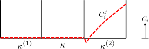
Figure 4.1: Schematic of an example scenario in which $\overline{C}_{i,\kappa,v}^{j+1}<0$ using the formulation described thus far.

Remark 14.

In the density limiter (see Section 4.3), if $\omega^{(1)}=1$, the limiter has no effect. If $\omega^{(1)}=0$, which corresponds to maximum limiter strength, then $C_{i}\leftarrow C_{i}^{(1)}=\overline{C}_{i},\;\forall i$, i.e., the species concentrations are projected to a $p=0$ representation. Suppose that $\grave{C}_{i,\kappa}^{j}\left(\xi\left(\zeta_{l}^{\left(f\right)}\right)\right)<0$, in which case $\overline{C}_{i,\kappa}^{j}>0$ by Remark 12. Applying the density limiter with $\omega^{(1)}=0$ then yields $\grave{C}_{i,\kappa}^{j,(1)}\left(x\right)=\overline{C}_{i,\kappa}^{j}>0,\>\forall x\in\partial\mathcal{D}_{\kappa}$.

Remark 15.

Suppose that $\overline{C}_{i,\kappa,v}^{j+1}<0$. Applying the density limiter to $y_{\kappa}^{j}$ with $\omega_{\kappa}^{(1)}=0$ and $y_{\kappa^{(f)}}^{j}$ with $\omega_{\kappa^{(f)}}^{(1)}=0,f=1,\ldots,n_{f}$ yields

$$\overline{C}_{i,\kappa,v}^{j+1,(1)}= \sum_{q=1}^{n_{q}}\theta_{q}\overline{C}_{i,\kappa}^{j}\left(\xi_{q}\right)$$

$$+\sum_{f=1}^{n_{f}}\sum_{l=1}^{n_{q,f}^{\partial}}\frac{\Delta t^{*}\nu_{f,l}^{\partial}}{2|\kappa|}\beta_{f,l}\overline{C}_{i,\kappa^{\left(f\right)}}^{j}\left(\xi\left(\zeta_{l}^{\left(f\right)}\right)\right)$$

$$+\sum_{f=1}^{n_{f}}\sum_{l=1}^{n_{q,f}^{\partial}}\Lambda_{f,l}\overline{C}_{i,\kappa}^{j}\left(\xi\left(\zeta_{l}^{\left(f\right)}\right)\right),$$

which is positive.

Remark 16.

$\mathcal{F}_{C_{i}}^{v}$ is directly proportional to $\nabla C$, i.e.,

$$\mathcal{F}_{C_{i},k}^{v}\left(y,\omega\nabla C\right) =\bar{D}_{i}\omega\frac{\partial C_{i}}{\partial x_{k}}-\frac{C_{i}\bar{D}_{i}}{\rho}\omega\frac{\partial\rho}{\partial x_{k}}-\frac{C_{i}}{\rho}\sum_{l=1}^{n_{s}}W_{l}\left(\bar{D}_{l}\omega\frac{\partial C_{l}}{\partial x_{k}}-\frac{C_{l}\bar{D}_{l}}{\rho}\omega\frac{\partial\rho}{\partial x_{k}}\right)$$

$$=\omega\left[\bar{D}_{i}\frac{\partial C_{i}}{\partial x_{k}}-\frac{C_{i}\bar{D}_{i}}{\rho}\frac{\partial\rho}{\partial x_{k}}-\frac{C_{i}}{\rho}\sum_{l=1}^{n_{s}}W_{l}\left(\bar{D}_{l}\frac{\partial C_{l}}{\partial x_{k}}-\frac{C_{l}\bar{D}_{l}}{\rho}\frac{\partial\rho}{\partial x_{k}}\right)\right]$$

$$=\omega\mathcal{F}_{C_{i},k}^{v}\left(y,\nabla C\right),$$

where $\omega$ is a scaling factor for $\nabla C$.

By Remark 15, a foolproof but low-fidelity approach to guarantee nonnegative species concentrations is as follows: if $\overline{C}_{i,\kappa,v}^{j+1}<0$, then apply a $p=0$ projection and recalculate $y_{\kappa,v}^{j+1}$, as well as the neighboring states. However, a higher-fidelity approach is desired. Following Remark 16, one such approach is to modify the gradient in the fourth term in Equation (3.2) as

$$\left(\left\{\!\!\left\{\mathcal{F}^{v}\left(y,\nabla y\right)\right\}\!\!\right\}\cdot n-\delta^{v}\left(y,\nabla y,n\right),\left\llbracket\mathfrak{v}\right\rrbracket\right)_{\epsilon}\leftarrow\left(\left\{\!\!\left\{\mathcal{F}^{v}\left(y,\omega\nabla y\right)\right\}\!\!\right\}\cdot n-\delta^{v}\left(y,\nabla y,n\right),\left\llbracket\mathfrak{v}\right\rrbracket\right)_{\epsilon},$$ (4.46)

where $\omega\in\left[0,1\right]$ is a pointwise parameter that scales the gradient. Specifically, for a given $\xi\left(\zeta_{l}^{\left(f\right)}\right)$, we have $\omega_{\kappa,l}^{(f)}$ and $\omega_{\kappa^{(f)},l}^{(f)}$ for the interior and exterior gradients, respectively, which yields

$$\grave{C}_{i,\kappa}^{j}\left(\xi\left(\zeta_{l}^{\left(f\right)}\right)\right)=C_{i,\kappa}^{j}\left(\xi\left(\zeta_{l}^{\left(f\right)}\right)\right)+\frac{\Delta t^{*}\nu_{f,l}^{\partial}}{2|\kappa|}\Lambda_{f,l}^{-1}\omega_{\kappa,l}^{(f)}\mathcal{F}_{C_{i}}^{v}\left(y_{\kappa}^{j}\left(\xi\left(\zeta_{l}^{\left(f\right)}\right)\right),\nabla C_{\kappa}^{j}\left(\xi\left(\zeta_{l}^{\left(f\right)}\right)\right)\right)\cdot n\left(\zeta_{l}^{\left(f\right)}\right)$$ (4.47)

and

$$\grave{C}_{i,\kappa^{\left(f\right)}}^{j}\left(\xi\left(\zeta_{l}^{\left(f\right)}\right)\right)=C_{i,\kappa^{(f)}}^{j}\left(\xi\left(\zeta_{l}^{\left(f\right)}\right)\right)+\beta_{f,l}^{-1}\omega_{\kappa^{(f)},l}^{(f)}\mathcal{F}_{C_{i}}^{v}\left(y_{\kappa^{(f)}}^{j}\left(\xi\left(\zeta_{l}^{\left(f\right)}\right)\right),\nabla C_{\kappa^{(f)}}^{j}\left(\xi\left(\zeta_{l}^{\left(f\right)}\right)\right)\right)\cdot n\left(\zeta_{l}^{\left(f\right)}\right).$$ (4.48)

This is akin to applying the linear-scaling limiter in Section 4.3 to only the gradient. In order to guarantee $\overline{C}_{i,\kappa,v}^{j+1}\geq 0$, $\omega_{\kappa,l}^{(f)}$ and $\omega_{\kappa^{(f)},l}^{(f)}$ in Equations (4.47) and (4.48) can be prescribed as

$$\omega_{\kappa,l}^{(f)}=\min_{i}\omega_{i,\kappa,l}^{(f)},\quad\omega_{i,\kappa,l}^{(f)}=\begin{cases}1,&Q_{i,\kappa,l}^{(f)}\geq 0,\\ -\frac{\frac{1}{2\sum_{f}n_{q,f}^{\partial}}\sum_{q=1}^{n_{q}}\theta_{q}C_{i,\kappa}^{j}\left(\xi_{q}\right)+\Lambda_{f,l}C_{i,\kappa}^{j}\left(\xi\left(\zeta_{l}^{\left(f\right)}\right)\right)}{\frac{\Delta t^{*}\nu_{f,l}^{\partial}}{2|\kappa|}\mathcal{F}_{C_{i}}^{v}\left(y_{\kappa}^{j}\left(\xi\left(\zeta_{l}^{\left(f\right)}\right)\right),\nabla C_{\kappa}^{j}\left(\xi\left(\zeta_{l}^{\left(f\right)}\right)\right)\right)\cdot n\left(\zeta_{l}^{\left(f\right)}\right)},&\mathrm{otherwise},\end{cases}$$ (4.49)

and

$$\omega_{\kappa^{(f)},l}^{(f)}=\min_{i}\omega_{i,\kappa^{(f)},l}^{(f)},\quad\omega_{i,\kappa^{(f)},l}^{(f)}=\begin{cases}1,&Q_{i,\kappa^{(f)},l}^{(f)}\geq 0,\\ -\frac{\frac{1}{2\sum_{f}n_{q,f}^{\partial}}\sum_{q=1}^{n_{q}}\theta_{q}C_{i,\kappa}^{j}\left(\xi_{q}\right)+\frac{\Delta t^{*}\nu_{f,l}^{\partial}}{2|\kappa|}\beta_{f,l}C_{i,\kappa^{\left(f\right)}}^{j}\left(\xi\left(\zeta_{l}^{\left(f\right)}\right)\right)}{\frac{\Delta t^{*}\nu_{f,l}^{\partial}}{2|\kappa|}\mathcal{F}_{C_{i}}^{v}\left(y_{\kappa^{(f)}}^{j}\left(\xi\left(\zeta_{l}^{\left(f\right)}\right)\right),\nabla C_{\kappa^{(f)}}^{j}\left(\xi\left(\zeta_{l}^{\left(f\right)}\right)\right)\right)\cdot n\left(\zeta_{l}^{\left(f\right)}\right)},&\mathrm{otherwise},\end{cases}$$ (4.50)

respectively, where $Q_{i,\kappa,l}^{(f)}$ and $Q_{i,\kappa^{(f)},l}^{(f)}$ are defined as

$$Q_{i,\kappa,l}^{(f)}= \frac{1}{2\sum_{f}n_{q,f}^{\partial}}\sum_{q=1}^{n_{q}}\theta_{q}C_{i,\kappa}^{j}\left(\xi_{q}\right)+\Lambda_{f,l}C_{i,\kappa}^{j}\left(\xi\left(\zeta_{l}^{\left(f\right)}\right)\right)$$

$$+\frac{\Delta t^{*}\nu_{f,l}^{\partial}}{2|\kappa|}\mathcal{F}_{C_{i}}^{v}\left(y_{\kappa}^{j}\left(\xi\left(\zeta_{l}^{\left(f\right)}\right)\right),\nabla C_{\kappa}^{j}\left(\xi\left(\zeta_{l}^{\left(f\right)}\right)\right)\right)\cdot n\left(\zeta_{l}^{\left(f\right)}\right),$$

$$Q_{i,\kappa^{(f)},l}^{(f)}= \frac{1}{2\sum_{f}n_{q,f}^{\partial}}\sum_{q=1}^{n_{q}}\theta_{q}C_{i,\kappa}^{j}\left(\xi_{q}\right)+\frac{\Delta t^{*}\nu_{f,l}^{\partial}}{2|\kappa|}\beta_{f,l}C_{i,\kappa^{\left(f\right)}}^{j}\left(\xi\left(\zeta_{l}^{\left(f\right)}\right)\right)$$

$$+\frac{\Delta t^{*}\nu_{f,l}^{\partial}}{2|\kappa|}\mathcal{F}_{C_{i}}^{v}\left(y_{\kappa^{(f)}}^{j}\left(\xi\left(\zeta_{l}^{\left(f\right)}\right)\right),\nabla C_{\kappa^{(f)}}^{j}\left(\xi\left(\zeta_{l}^{\left(f\right)}\right)\right)\right)\cdot n\left(\zeta_{l}^{\left(f\right)}\right),$$

such that $\overline{C}_{i,\kappa,v}^{j+1}$ in Equation (4.45) can be rewritten as

$$\overline{C}_{i,\kappa,v}^{j+1}=\sum_{f=1}^{n_{f}}\sum_{l=1}^{n_{q,f}^{\partial}}Q_{i,\kappa,l}^{(f)}+\sum_{f=1}^{n_{f}}\sum_{l=1}^{n_{q,f}^{\partial}}Q_{i,\kappa^{(f)},l}^{(f)}.$$

$\beta_{f,l}$ can then be prescribed using only the $\beta_{T}$ constraint (4.5) (i.e., the constraint (4.6) can be ignored); furthermore, $\beta_{f,l}$ does not need to be recomputed since $\mathcal{F}^{v}\left(y,\omega\nabla y\right)=G\left(y\right):\omega\nabla y=\omega\mathcal{F}^{v}\left(y,\nabla y\right)$ and $\beta^{*}\left(y,\mathcal{F}^{v}\left(y,\nabla y\right),n\right)\geq\beta^{*}\left(y,\omega\mathcal{F}^{v}\left(y,\nabla y\right),n\right)=\omega\beta^{*}\left(y,\mathcal{F}^{v}\left(y,\nabla y\right),n\right)$, for $\omega\in\left[0,1\right]$. It should also be noted that the constraint (4.6) can be overly restrictive, such that nonnegativity of species concentrations can often be maintained even if the constraint (4.6) is neglected and $\omega_{\kappa,l}^{(f)}=\omega_{\kappa^{(f)},l}^{(f)}=1$ for all $l,f$. In general, the need to limit the gradient seems to be extremely rare. In fact, such gradient limiting is not needed for the results presented here (i.e., the adaptive time stepping procedure was sufficient); however, it will quickly become necessary if, for example, insufficient artificial viscosity is applied to the moving-detonation test described in Section 5.4. In practice, an appropriate strategy is to limit the gradient when $\overline{C}_{i,\kappa,v}^{j+1}<0$ and excessive loops are taken in the adaptive time stepping procedure. An alternative to (4.46) is to instead apply the density limiter in Section 4.3 to the state and modify the fourth term in Equation (3.2) as

$$\left(\left\{\!\!\left\{\mathcal{F}^{v}\left(y,\nabla y\right)\right\}\!\!\right\}\cdot n-\delta^{v}\left(y,\nabla y,n\right),\left\llbracket\mathfrak{v}\right\rrbracket\right)_{\epsilon}\leftarrow\left(\left\{\!\!\left\{\mathcal{F}^{v}\left(\ddot{y},\nabla\ddot{y}\right)\right\}\!\!\right\}\cdot n-\delta^{v}\left(\ddot{y},\nabla\ddot{y},n\right),\left\llbracket\mathfrak{v}\right\rrbracket\right)_{\epsilon},$$ (4.51)

where

$$\ddot{y}=\left(\rho v_{1},\ldots,\rho v_{d},\rho e_{t},\ddot{C_{1}},\ldots,\ddot{C}_{n_{s}}\right),\quad\ddot{C_{i}}=\overline{C}_{i}+\omega\left(C_{i}-\overline{C}_{i}\right).$$

However, iteration would then be required to determine $\omega_{\kappa,l}^{(f)}$ and $\omega_{\kappa^{(f)},l}^{(f)}$ such that $\overline{C}_{i,\kappa,v}^{j+1}\geq 0$.

5 Results

We consider three one-dimensional test cases: advection-diffusion of a thermal bubble, a premixed flame, and viscous shock-tube flow. Next, we compute two multidimensional reacting flows: a moving detonation wave enclosed by adiabatic walls and shock/mixing-layer interaction. Unless otherwise specified, the positivity-preserving, entropy-bounded DG formulation presented in the previous section, along with the adaptive time stepping strategy described in Section 4.6, is employed. All simulations are performed using a modified version of the JENRE® Multiphysics Framework [50, 2] that incorporates the developments and extensions described in this work. Unless otherwise specified, the second-order strong-stability-preserving Runge-Kutta method (SSPRK2) [37, 38] is employed.

5.1 One-dimensional thermal bubble advection-diffusion

In this problem, we assess the order of accuracy of the positivity-preserving and entropy-bounded DG formulation (without artificial viscosity). The computational domain is $\Omega=[-25,25]\>\mathrm{m}$. Periodicity is imposed at the left and right boundaries. The initial conditions are given by

$$v_{1} = 1\textrm{ m/s},$$

$$Y_{H_{2}} = \frac{1}{2}\left[1-\tanh\left(|x|-10\right)\right],$$

$$Y_{O_{2}} = 1-Y_{H_{2}},$$ (5.1)

$$T = 1200-900\tanh\left(|x|-10\right)\textrm{ K},$$

$$P = 1\textrm{ bar}.$$

In [2], optimal convergence without any additional stabilization, including limiting, was demonstrated. In [10], we showed optimal convergence from $p=1$ to $p=3$ using the positivity-preserving, entropy-bounded DG method for inviscid, reacting flows. Four element sizes were considered: $h$, $h/2$, $h/4$, and $h/8$, where $h=2\>\mathrm{m}$. The limiters were not activated when finer meshes were employed. Here, we repeat this investigation in the viscous setting. Instead of the adaptive time stepping strategy described in Section 4.6, we separately consider both viscous flux functions with fixed $\mathrm{CFL}=0.1$. The “exact” solution is obtained with $p=3$ and $h/256$. The $L^{2}$ error at $t=5\>\mathrm{s}$ is computed in terms of the normalized state variables,

$$\widehat{\rho v}_{k}=\frac{1}{\sqrt{\rho_{r}P_{r}}}\rho v_{k},\quad\widehat{\rho e}_{t}=\frac{1}{P_{r}}\rho e_{t},\quad\widehat{C}_{i}=\frac{R^{0}T_{r}}{P_{r}}C_{i},$$

where $\rho_{r}=1\,\mathrm{kg\cdot}\mathrm{m}^{-3}$, $T_{r}=1000\,\mathrm{K}$, and $P_{r}=101325\,\mathrm{Pa}$. Figure 5.1 shows the convergence results for both viscous flux functions. The theoretical convergence rates are denoted with dashed lines. The “$\times$” symbol indicates that the positivity-preserving limiter is activated, the “$\Circle$” symbol indicates that the entropy limiter is activated, and the “$\triangle$” symbol indicates that neither limiter is activated. If both limiters are activated, then the corresponding symbols are superimposed as “$\otimes$”. The results are extremely similar between the two viscous flux functions. Apart from the coarser grids with $p=1$, which are likely outside the asymptotic regime, optimal convergence is demonstrated. For $h$ and $h/2$, both limiters are activated across all $p$; for $h/4$ and $p=1$, only the positivity-preserving limiter is activated. At higher resolutions, the limiters are not engaged since the solutions are fairly well-resolved.

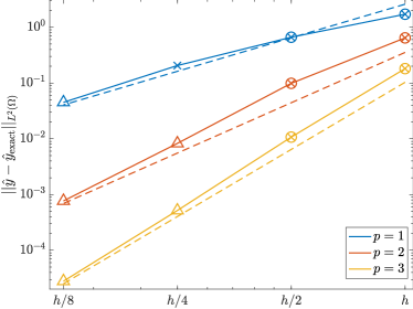
(a) BR2 viscous flux function.

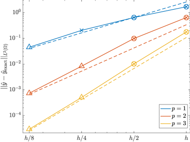
(b) Lax-Friedrichs-type viscous flux function.

Figure 5.1: Convergence under grid refinement, with $h=2\>\mathrm{m}$, for the one-dimensional thermal bubble test case. The $L^{2}$ error of the normalized state with respect to the exact solution at $t=5\>\mathrm{s}$ is computed. The dashed lines represent the theroretical convergence rates. The “$\times$” symbol indicates that the positivity-preserving limiter is activated, the “$\Circle$” symbol indicates that the entropy limiter is activated, and the “$\triangle$” symbol indicates that neither limiter is activated. If both limiters are activated, then the corresponding symbols are superimposed as “$\otimes$”.

5.2 One-dimensional premixed flame 

In this problem, we consider a smooth, viscous flow with chemical reactions. A freely propagating flame is calculated in Cantera [30] on a 1 cm long grid using the left state in Equations (5.2) and (5.3) below. The computational domain is $\Omega=[0,0.01]\text{ m}$. For the DG calculations, we generate a mesh that contains a refinement zone between 1.8 mm and 2.5 mm with grid spacing $h=200$ $\mu$m, a target size that is 200 times larger than the smallest grid spacing from the resulting refinement procedure in Cantera. The mesh transitions to a spacing of $500$ $\mu$m at the boundaries. The objective here is to ignite the flame and establish a solution in which the flame anchors itself in the fine region of the one-dimensional mesh. The initial conditions are given by

$$\left(v_{1},T,P\right) = \begin{cases}\left(9.53\text{ m/s},2122\text{ K},1\text{ atm},\right),&x\geq 0.0025\\ \left(1.53\text{ m/s},300\text{ K},1\text{ atm},\right),&x<0.0025\end{cases},$$ (5.2)

with mass fractions

$$\begin{split}\left(Y_{H_{2}},Y_{O_{2}},Y_{N_{2}},Y_{H},Y_{O}\right)=&\begin{cases}\left(7\times 10^{-5},0.0572,0.745,4.2\times 10^{-6},2.2\times 10^{-4}\right),&x\geq 0.0025\\ \left(0.023,0.24,0.737,0,0\right),&x<0.0025\end{cases}\\ \left(Y_{OH},Y_{H_{2}O},Y_{HO_{2}},Y_{H_{2}O_{2}}\right)=&\begin{cases}\left(2.7\times 10^{-4},0.194,3\times 10^{-6},2.1\times 10^{-7}\right),&x\geq 0.0025\\ \left(0,0,0,0\right),&x<0.0025\end{cases}\end{split}.$$ (5.3)

The right state corresponding to $x\geq 0.0025$ m is the final fully reacted state from the Cantera solution. The left boundary condition is a characteristic inflow condition that allows pressure waves to leave the domain. The right boundary is a reflective outflow condition with the pressure set to 1 atm.

In the beginning of the simulation, the states on both sides of the discontinuity immediately diffuse to form a smooth profile. As the reactions progress, the flame accelerates against the right-moving reactants and then slows down to the flame speed. With sufficient accuracy, the flame should remain stationary inside the refined region. The default CFL is set to 0.4. We perform $p=1$ and $p=3$ calculations both with the proposed formulation and with conventional species clipping (instead of the positivity-preserving and entropy limiters), in which negative species concentrations are simply set to zero. Artificial viscosity is not employed in these calculations.

Figure  5.2 shows instantaneous solutions at $t=0.012566$ s for $p=1$ , obtained with species clipping. Clear discrepancies between the solution and the Cantera solution are observed. The mass fractions of the intermediate species, namely $HO_{2}$ and $H_{2}O_{2}$, are over-predicted. Additionally, the pressure deviates from the expected ambient pressure by a factor of approximately $50\times 10^{-4}$, with sharp structural changes prior to the flame front. Beyond the poor predictive abilities with species clipping, the solution fails to maintain a stable profile; by $t=0.02$ s, the flame drifts out of the refinement zone.

The results obtained for $p=1$ and $p=3$ with the proposed positivity-preserving, entropy-bounded methodology are given in Figures 5.3a and 5.3b, respectively. The $p=1$ solution does not fully capture the species profiles, and the pressure oscillates through the flame; nevertheless, it agrees much more closely with the Cantera solution than the $p=1$ solution obtained with species clipping. The $p=3$ solution at the given time is in much better agreement to the species profiles of the Cantera solution than the $p=1$ solution. The $p=3$ pressure solution smoothly transitions through the flame without the spikes found in the $p=1$ solution. A slight pressure change through the flame is expected given a compressible formulation. A major improvement over the the clipping solution is that, in both the $p=1$ and $p=3$ simulations, the flame is held in the refinement zone, achieving the desired steady state flame at the expected flame speed. These results illustrate the significant benefits of employing the proposed positivity-preserving, entropy-bounded DG formulation.

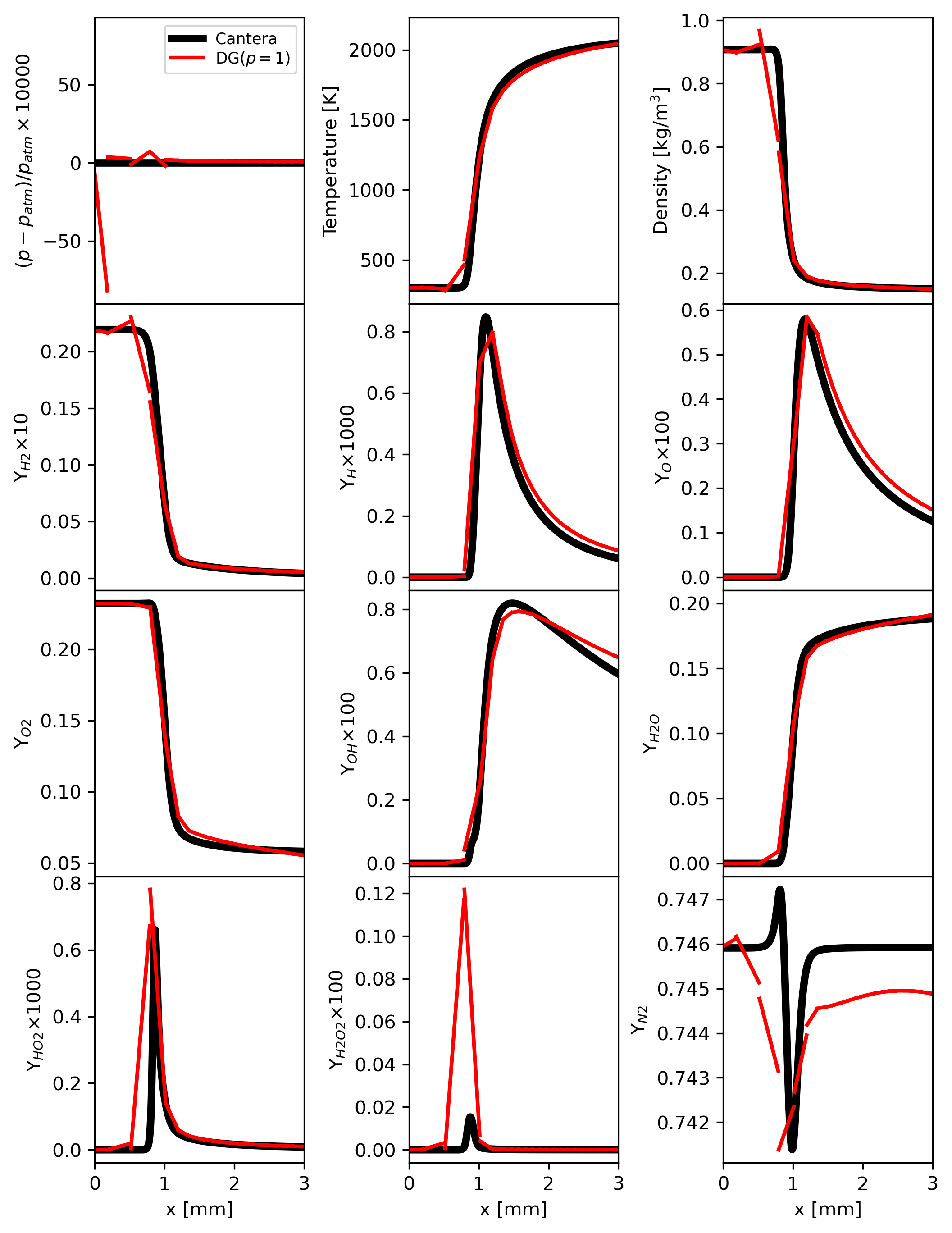
Figure 5.2: Solution for a one-dimensional premixed flame at $t=0.012566$ s obtained with species clipping. The $p=1$ solutions drift out of the refinement zone by $t=2$ s.

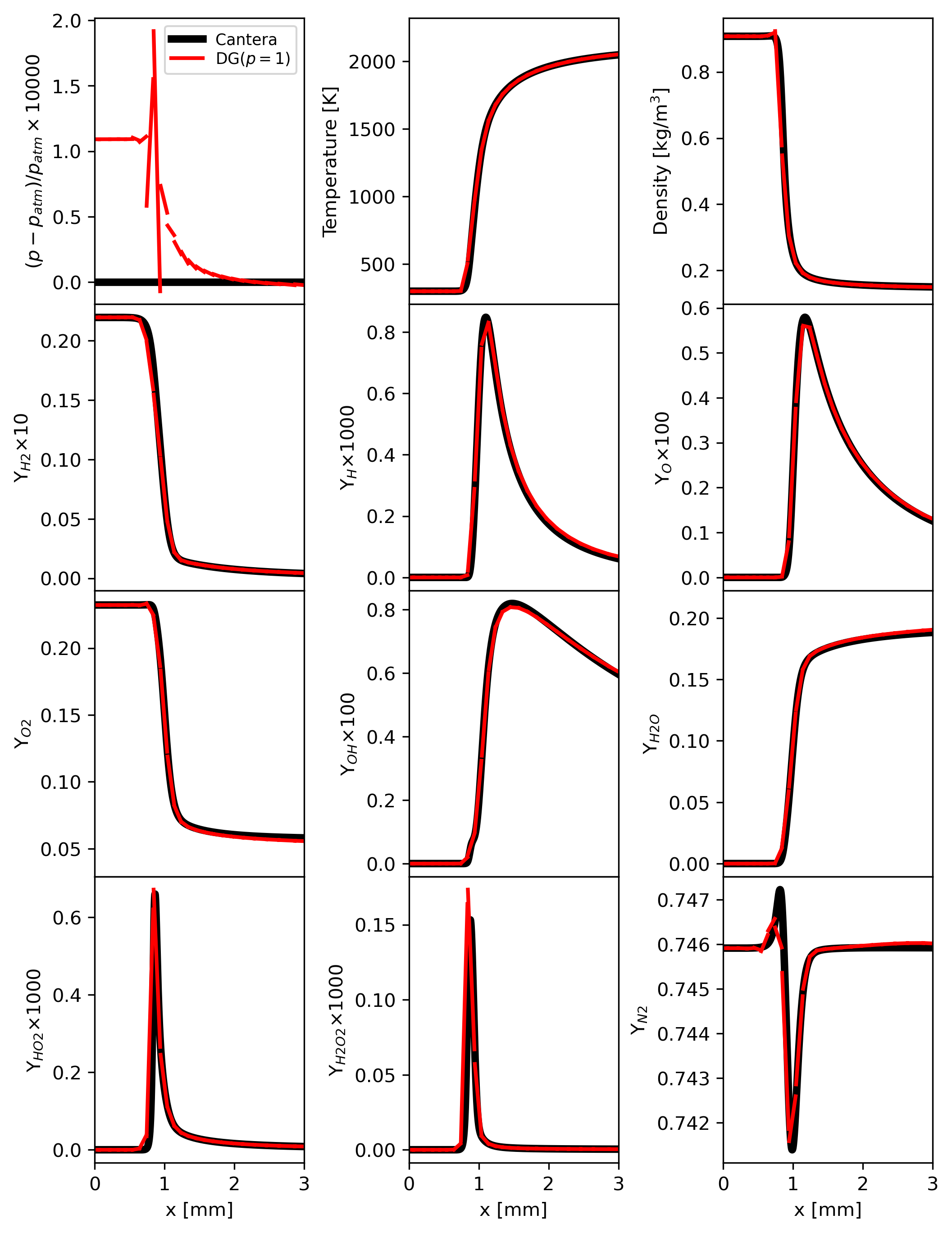
(a) $p=1$

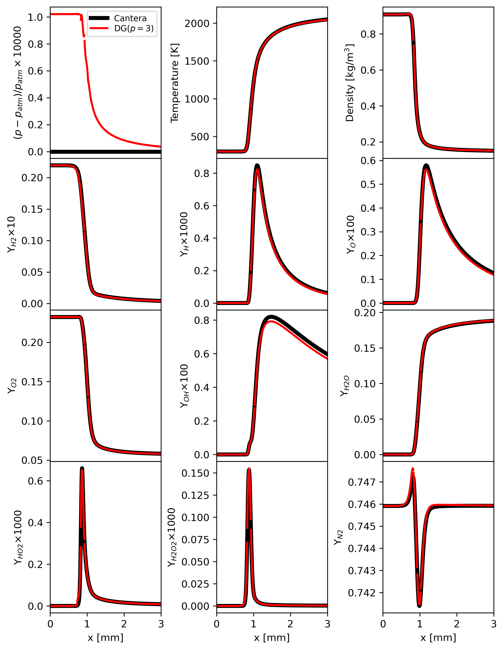
(b) $p=3$

Figure 5.3: Solutions for a one-dimensional premixed flame at $t=0.012566$ s obtained with the proposed positivity-preserving, entropy-bounded formulation.

5.3 One-dimensional shock tube

This test case was computed without viscous effects by Houim and Kuo [27], by Johnson and Kercher [2], and in our previous work [10], where we showed that (a) instabilities in the multicomponent, thermally perfect case are much greater than in the monocomponent, calorically perfect case and (b) enforcement of an entropy bound suppresses large-scale nonphysical oscillations much more effectively than enforcement of the positivity property. Our goals here are to investigate whether these observations hold in the viscous setting and to further compare the BR2 and Lax-Friedrichs-type viscous flux functions. The computational domain is $\Omega=[0,1]\text{ m}$, and the final time is $t=300\;\mu\mathrm{s}$. Walls are imposed at the left and right boundaries. The initial conditions are written as

$$\left(v_{1},T,P,Y_{N_{2}},Y_{He}\right)=\begin{cases}\left(0\text{ m/s},300\text{ K},1\text{ atm},1,0\right),&x\geq 0.4\\ \left(0\text{ m/s},300\text{ K},10\text{ atm},0,1\right),&x<0.4\end{cases}.$$ (5.4)

The default CFL is set to 0.1. For the remainder of this subsection, “BR2” refers to the adaptive time stepping strategy exactly as described in Section 4.6, whereas “LLF” refers to a similar time stepping strategy, but with the viscous flux function fixed to be the local Lax-Friedrichs-type flux function. In addition, “PPL” corresponds to only the positivity-preserving limiter, while “EL” corresponds to both the positivity-preserving and entropy limiters. Based on [2] and [10], a reference solution is computed using $p=2$, 2000 elements, artificial viscosity, BR2, and EL. All other solutions are computed using $p=3$ and 200 elements.

Figure 5.4 shows the mass fraction, pressure, temperature, and entropy profiles obtained with BR2. Except for the reference solution, artificial viscosity is not employed in order to isolate the effects of the limiters. Note that the linear-scaling limiters alone are not expected to eliminate small-scale spurious oscillations [13, 12, 41, 42]. The results are very similar to those in the inviscid case [10]. The species profiles are well-captured using both types of limiting. The entropy limiter dampens large-scale instabilities in the pressure, temperature, and entropy distributions significantly better than the positivity-preserving limiter. Furthermore, just as observed in [10], the instabilities still present with the positivity-preserving limiter are substantially larger than those usually present in monocomponent, calorically perfect shock-tube solutions computed with the positivity-preserving limiter [13, 47, 16], and the relative advantage of applying the entropy limiter is much greater. The addition of artificial viscosity would greatly suppress the small-scale instabilities; for brevity, such results are not included here, but they are very similar to those in [10]. At the same time, artificial viscosity alone (without the limiters) results in negative concentrations and other instabilities, thus motivating a combination of the two stabilization mechanisms. The corresponding LLF results are given in Figure 5.5, which are very similar to the BR2 results. However, the temperature overshoot at the shock is noticeably smaller in the LLF case, indicating that the Lax-Friedrichs-type viscous flux function can sometimes have better stabilization properties than the BR2 scheme. Regardless, the results in the following subsection suggest that the latter is still the preferred viscous flux function, provided that the positivity property is satisfied.

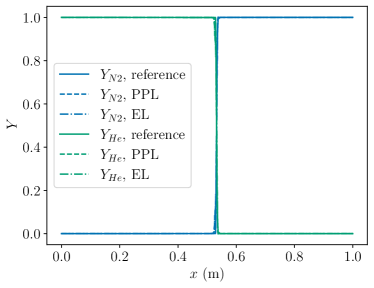
(a) Mass fractions.

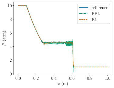
(b) Pressure.

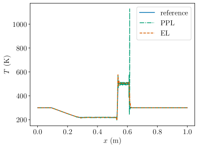
(c) Temperature.

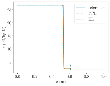
(d) Specific thermodynamic entropy.

Figure 5.4: Results for $p=3$ solutions computed using BR2 on 200 elements without artificial viscosity for the one-dimensional, multicomponent shock-tube problem with initialization in Equation (5.4). “PPL” corresponds to the positivity-preserving limiter by itself, and “EL” refers to both the positivity-preserving and entropy limiters with the local entropy bound in Equation (4.20).

(a) Mass fractions.

(b) Pressure.

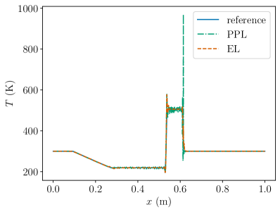
(c) Temperature.

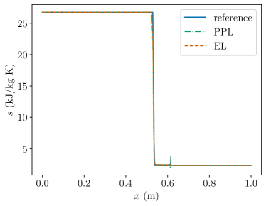
(d) Specific thermodynamic entropy.

Figure 5.5: Results for $p=3$ solutions computed using LLF on 200 elements without artificial viscosity for the one-dimensional, multicomponent shock-tube problem with initialization in Equation (5.4). “PPL” corresponds to the positivity-preserving limiter by itself, and “EL” refers to both the positivity-preserving and entropy limiters with the local entropy bound in Equation (4.20).

Figure 5.6 presents the percent error in mass, energy, and atom conservation for the BR2, EL solution as a representative example, calculated every $0.3\;\mu\mathrm{s}$ (for a total of 1000 samples). $\mathsf{N}_{N}$ and $\mathsf{N}_{He}$ denote the total numbers of nitrogen and helium atoms in the mixture. The error remains close to machine precision, verifying that the developed DG framework is conservative. Also shown is the error in mass conservation (calculated every time step) for a solution computed with conventional species clipping. The error rises considerably before the solver diverges.

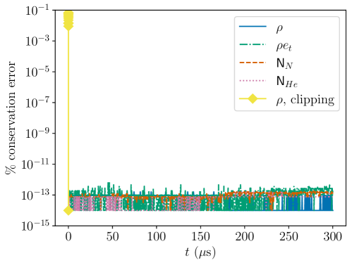
Figure 5.6: Percent error in mass, energy, and atom conservation for the “EL” case in Figure 5.4, computed with $p=3$ on 200 elements. The initial conditions for this one-dimensional, multicomponent shock-tube problem are given in Equation (5.4). Also shown is the error in mass conservation for a solution computed with conventional species clipping.

5.4 Two-dimensional detonation wave 

This test case involves a moving hydrogen-oxygen detonation wave diluted in Argon with initial conditions

$$\begin{array}[]{cccc}\qquad\qquad\qquad\left(v_{1},v_{2}\right)&=&\left(0,0\right)\text{ m/s},\\ X_{Ar}:X_{H_{2}O}:X_{OH}:X_{O_{2}}:X_{H_{2}}&=&\begin{cases}8:2:0.1:0:0\\ 7:0:0:1:2\end{cases}&\begin{array}[]{c}x_{1}<0.015\text{ m},x\in\mathcal{C}_{1},x\in\mathcal{C}_{2}\\ \mathrm{otherwise}\end{array},\\ \qquad\qquad\qquad\qquad P&=&\begin{cases}{5.50}\mathrm{e}{5}&\text{ Pa}\\ {6.67}\mathrm{e}{3}&\text{ Pa}\end{cases}&\begin{array}[]{c}x_{1}<0.015\text{ m},x\in\mathcal{C}_{1},x\in\mathcal{C}_{2}\\ \mathrm{otherwise}\end{array},\\ \qquad\qquad\qquad\qquad T&=&\begin{cases}3500&\text{ K}\\ 300\text{\hskip 10.00002pt\hskip 10.00002pt}&\text{ K}\end{cases}&\begin{array}[]{c}x_{1}<0.015\text{ m},x\in\mathcal{C}_{1},x\in\mathcal{C}_{2}\\ \mathrm{otherwise}\end{array},\end{array}$$ (5.5)

where

$$\mathcal{C}_{1} =\left\{x\left|\sqrt{\left(x_{1}-0.021\right)^{2}+\left(x_{2}-0.015\right)^{2}}<0.0025\text{ m}\right.\right\},$$

$$\mathcal{C}_{2} =\left\{x\left|\sqrt{\left(x_{1}-0.022\right)^{2}+\left(x_{2}-0.044\right)^{2}}<0.0025\text{ m}\right.\right\},$$

which represent two high-pressure/high-temperature regions to perturb the flow. The computational domain is $\text{$\Omega$}=\left(0,0.45\right)\mathrm{m}\times\left(0,0.06\right)\mathrm{m}$, with adiabatic, no-slip walls at the left, right, bottom, and top boundaries. The Westbrook mechanism [51] is employed.

Johnson and Kercher computed this flow without viscous effects with $p=1$ and a very fine mesh with spacing $h=9\times 10^{-5}$ m [2]. In [11], we simulated this flow (also without viscous effects) using a series of triangular grids ranging from very coarse to fine. Stability was maintained across all resolutions. The finer cases predicted the correct diamond-like cellular structure, with a cell length of $0.055\text{ m}$ and a cell height of $0.03\text{ m}$ [52, 53]. In particular, there were two cells in the vertical direction. Here, we recompute this flow with viscous effects and quadrilateral elements. Specifically, we use Gmsh [54] to first generate structured-type, uniform grids with element sizes of $2h$, $8h$, and $32h$; the cells are then clustered near the top and bottom walls, resulting in smaller mesh spacing in the vertical direction at said walls. Since the grids do not directly account for the circular perturbations in Equation (5.5), the discontinuities in the initial conditions are slightly smoothed using hyperbolic tangent functions. For the remainder of this subsection, “BR2” refers to the adaptive time stepping strategy exactly as described in Section 4.6, whereas “LLF” refers to a similar time stepping strategy, but with the viscous flux function fixed to be the local Lax-Friedrichs-type flux function. The default CFL is set to 0.3.

Figure 5.7 presents the distributions of OH mole fraction and temperature obtained from $p=2$ solutions at $t=200$ $\mu\mathrm{s}$ computed with LLF. Unsurprisingly, the $32h$ solution is extremely smeared behind the shock. Nonphysical oscillations are observed near the top and bottom walls. To more clearly illustrate these oscillations, Figure 5.8 (top) zooms in on the temperature field at the bottom wall. The flow is much better resolved in the $8h$ case according to Figure 5.7. The near-wall oscillations largely disappear, but spurious oscillations are present in the post-shock region, particularly around $x_{1}=0.1$ m in the mole-fraction field. Figure 5.9 displays the corresponding distributions of OH mole fraction and temperature obtained with BR2, along with a $2h$ solution. Figure 5.8 (bottom) gives the near-wall temperature distribution for $32h$. These $32h$ and $8h$ solutions are similar to the LLF solutions, but generally free from the aforementioned oscillations, which is why the BR2 flux function is chosen to be the “default” flux function in the adaptive time stepping strategy proposed in Section 4.6. The detonation-front locations are fairly close across all cases. In the $2h$ solution, the flow topology, including transverse waves, vortices, and triple points, is well-captured.

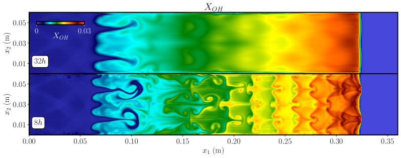
(a) OH mole fraction

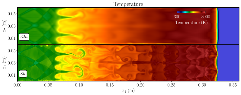
(b) Temperature

Figure 5.7: $p=2$ solution to a two-dimensional moving detonation wave at $t=200$ $\mu\mathrm{s}$ computed with LLF. The initial conditions are given in Equation (5.5).

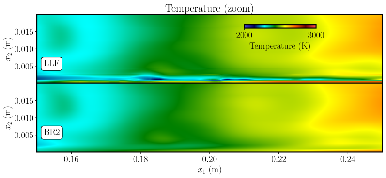
Figure 5.8: Temperature distributions obtained with the $32h$ mesh zoomed in on the bottom wall.

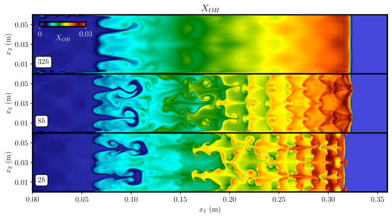
(a) OH mole fraction

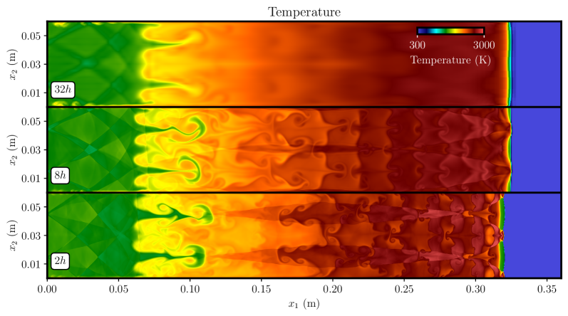
(b) Temperature

Figure 5.9: $p=2$ solution to a two-dimensional moving detonation wave at $t=200$ $\mu\mathrm{s}$ computed with BR2. The initial conditions are given in Equation (5.5).

Figure 5.10 presents the maximum-pressure history, $P^{*}$, where $P^{*,j+1}(x)=\max\left\{P^{j+1}(x),P^{*,j}(x)\right\}$, for the $p=2$, BR2 solutions, which reveals the expected cellular structure, with two cells in the vertical direction. The detonation cells in the $32h$ solution can be hardly discerned due to the excessive smearing. The cells in the $8h$ solution can be clearly discerned, but begin to dissipate towards the right of the domain. Finally, those in the $2h$ solution remain sharp throughout.

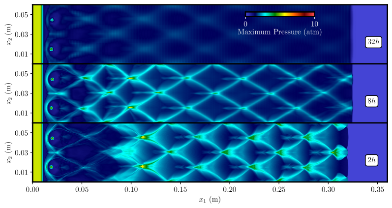
Figure 5.10: Maximum-pressure history, $P^{*}$, where $P^{*,j+1}(x)=\max\left\{P^{j+1}(x),P^{*,j}(x)\right\}$, for a two-dimensional moving detonation wave at $t=200$ $\mu\mathrm{s}$ computed with $p=2$, BR2, and a sequence of meshes, where $h=9\times 10^{-5}$ m. The initial conditions are given in Equation (5.5).

Figure 5.11 presents the percent error in discrete conservation of mass, energy, and atomic elements for BR2, $32h$ as a representative example, calculated every $0.200\;\mu\mathrm{s}$ (for a total of 1000 samples). $\mathsf{N}_{O}$, $\mathsf{N}_{H}$, and $\mathsf{N}_{Ar}$ denote the total numbers of oxygen, hydrogen, and argon atoms in the mixture. The errors remain close to machine precision throughout the simulation. The fluctuations and slight increases in the error profiles are largely a result of minor numerical-precision issues due to the different orders of magnitude among the state variables. These results confirm that the proposed DG formulation is fully conservative. Also given in Figure 5.11 is the error in mass conservation (calculated every time step) for a solution obtained with conventional species clipping. Artificial viscosity is still employed. The error increases rapidly until the solver diverges. We further note that if only the positivity-preserving limiter is employed (without the entropy limiter), then large-scale temperature undershoots may appear that can hinder convergence of the nonlinear solver in the reaction step. For example, the $32h$ calculation with the entropy limiter is nearly three times less expensive than a corresponding $32h$ calculation with solely the positivity-preserving limiter.

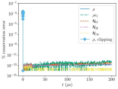
Figure 5.11: Percent error in mass, energy, and atom conservation for the $p=2$, BR2, $32h$ solution. The initial conditions for this two-dimensional hydrogen detonation problem are given in Equation (5.5). Also given is the error in mass conservation for a solution obtained with conventional species clipping.

Finally, we recompute the BR2, $32h$ case with curved elements of quadratic geometric order. Specifically, high-order geometric nodes are first inserted into the straight-sided mesh, after which the midpoint nodes at interior interfaces are perturbed. These perturbations are performed only for $x>0.05\text{ m}$ to ensure the initial conditions are the same. This low-resolution case is computed in order to guarantee that the limiter is frequently activated. Figure 5.12 displays the distributions of OH mole fraction for the linear and curved meshes, which are superimposed. The solution obtained with curved mesh is stable and extremely similar to that computed with the linear mesh, demonstrating that the proposed formulation is indeed compatible with curved elements.

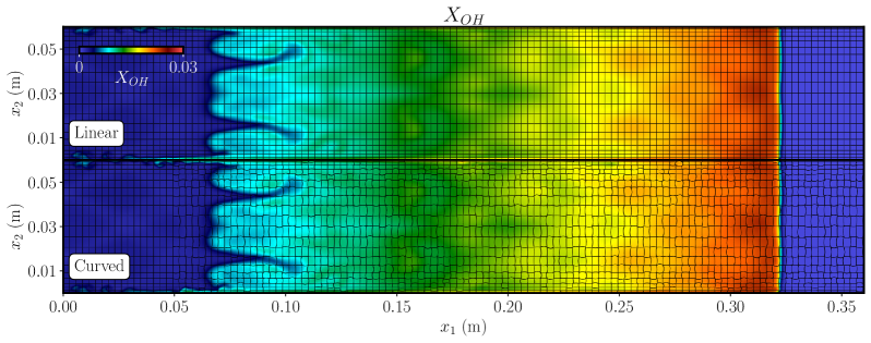
Figure 5.12: OH mole-fraction field for a two-dimensional moving detonation wave at $t=200$ $\mu\mathrm{s}$ computed with $p=2$, BR2, and $32h$, where $h=9\times 10^{-5}$ m, on linear and curved meshes. The curved mesh, which is of quadratic order, is obtained by inserting high-order geometric nodes into the linear mesh and perturbing said nodes. The initial conditions are given in Equation (5.5).

5.5 Three-dimensional shock/mixing-layer interaction

In this section, we compute a three-dimensional chemically reacting mixing layer that intersects an oblique shock. This test case was first presented in [55], which built on the configuration introduced in [56]. The mesh and flow parameters are slightly different from those in [55].

Figure 5.13 displays a two-dimensional schematic of the flow configuration. Supersonic inflow is applied at the left boundary, and extrapolation is applied at the right boundary. Flow parameters for the incoming air and fuel are listed in Table 1. Slip-wall conditions are applied the top and bottom walls since it is not necessary to capture the boundary layers. We employ the detailed reaction mechanism from Westbrook [51].

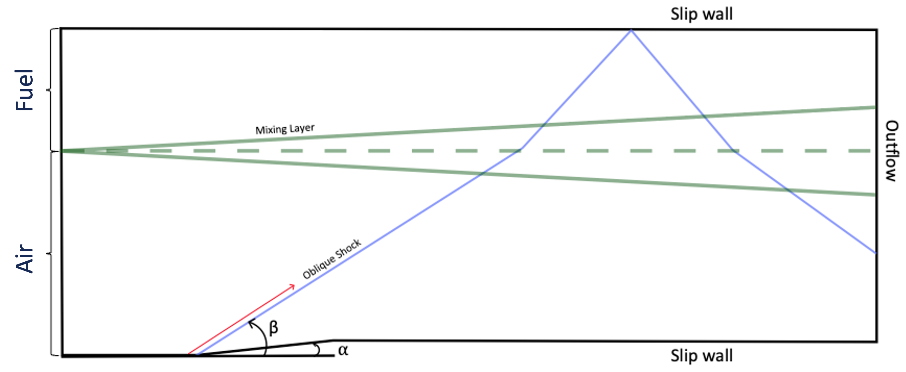
Figure 5.13: Schematic of the three-dimensional shock/mixing-layer interaction test case.

Prescribed Quantity	Air Boundary	Fuel Boundary
Velocity, $v_{1}$ [m/s]	1634 m/s	973 m/s
Temperature, $T$ [K]	1475	545
$Y_{O_{2}}$	0.278	0
$Y_{N_{2}}$	0.552	0.95
$Y_{H_{2}}$	0	0.05
$Y_{H_{2}O}$	0.17	0
$Y_{H}$	$5.6\times 10^{-7}$	0
$Y_{O}$	$1.55\times 10^{-4}$	0
$Y_{OH}$	$1.83\times 10^{-3}$	0
$Y_{HO_{2}}$	$5.1\times 10^{-6}$	0
$Y_{H_{2}O_{2}}$	$2.5\times 10^{-6}$	0

Table 1: Inflow parameters for three-dimensional shock/mixing-layer interaction. These values are taken from Fer14 [56].

To connect the fuel and air streams, we utilize a hyperbolic tangent function for prescribing the species, temperature, and normal direction velocity with a constant pressure specification,

$$Y_{i}(x_{1},\dots,x_{d},t) = \frac{1}{2}\left(\left(Y_{i,F}+Y_{i,O}\right)+\left(Y_{i,F}-Y_{i,O}\right)\tanh\left(\frac{\left(2\left(x_{2}-h\left(x_{1},\dots,x_{d},t\right)\right)\right)}{L\left(x_{1},\dots,x_{d},t\right)}\right)\right)$$

$$T(x_{1},\dots,x_{d},t) = \frac{1}{2}\left(\left(T_{F}+Y_{O}\right)+\left(T_{F}-T_{O}\right)\tanh\left(\frac{\left(2\left(x_{2}-h\left(x_{1},\dots,x_{d},t\right)\right)\right)}{L\left(x_{1},\dots,x_{d},t\right)}\right)\right)$$

$$v_{1}(x_{1},\dots,x_{d},t) = \frac{1}{2}\left(\left(v_{1,F}+v_{1,O}\right)+\left(v_{1,F}-v_{1,O}\right)\tanh\left(\frac{\left(2\left(x_{2}-h\left(x_{1},\dots,x_{d},t\right)\right)\right)}{L\left(x_{1},\dots,x_{d},t\right)}\right)\right)$$ (5.6)

$$P = 94232.25\text{ Pa},$$

where $(\cdot)_{O}$ denotes air, $(\cdot)_{F}$ denotes fuel, $L$ is a length scale, and $h$ is the center of the hyperbolic tangent. Equation 5.6 is also used to initialize the solution. $L$ is given by

$$L(x_{1},\dots,x_{d},t) = L_{s}+\sum_{i=1}^{n_{t}}A_{i}\sin\left(\frac{n_{i}2\pi t}{t_{r}}\right)+l(x_{1},\dots,x_{d})$$

$$l\left(x_{1},\dots,x_{d}\right) = \sum_{i=1}^{n_{v}}\sin\left(\frac{m_{i}2\pi x_{3}}{z_{h}}\right)\sum_{i=1}^{n_{w}}B_{i}\sin\left(\frac{q_{i}2\pi t}{t_{r}}\right)\text{,}$$ (5.7)

where $L_{s}=0.05$ mm is the ambient length scale; $A_{i}$ and $B_{i}$ are amplitudes; $n_{i}$, $m_{i}$, and $q_{i}$ are wavenumbers; $z_{h}=0.00144$ m is the domain thickness in the $x_{3}$-direction; $t_{r}=1.142\times 10^{-7}$ s is the flow-through time according to the air velocity; and $n_{t}=4$. This prescription of $L$ introduces unsteadiness while maintaining reproducibility. To induce variation in this three-dimensional case, we prescribe $h$ as

$$h(x_{1},\dots,x_{d},t) = h_{s}+h_{t}\sin\left(\frac{m_{0}2\pi x_{3}}{z_{h}}\right),$$ (5.8)

where $h_{s}$ is the ambient center of the hyperbolic tangent. Additional information can be found in Bur22 [55].

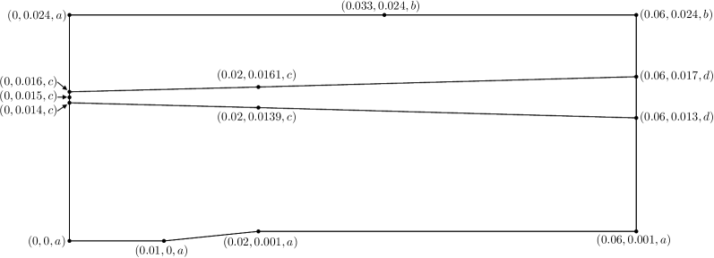
Figure 5.14: Diagram of geometry with point locations for mesh construction in Gmsh [54]. The third value in each tuple ($a$ through $d$) is the target mesh size at the respective locations.

Figure 5.14 shows the specifications in Gmsh [54] used to create an unstructured tetrahedral mesh. For each tuple, the first two values are the $x_{1}$ and $x_{2}$ locations of the given point. The third value represents the target mesh size. We select $a=500\times 10^{-6}$ m, $b=200\times 10^{-6}$ , $c=60\times 10^{-6}$ , and $d=120\times 10^{-6}$ m. The mesh is extruded in the $x_{3}$-direction from $x_{3}=0$ to $x_{3}=z_{h}$, with periodicity applied at the resulting $x_{1}x_{2}$-planes.

Figure 5.15 shows isosurfaces corresponding to $Y_{OH}=0.00017$, superimposed on a numerical Schlieren result sampled along an $x_{1}x_{2}$-plane. The $Y_{OH}$ isosurfaces ares colored by pressure to highlight the abrupt compression experienced through the oblique shock. The right image provides a zoomed-in perspective to emphasize the three dimensional flow features. Roll-up is observed upstream of the oblique shock. The interaction between the shock and the mixing layer causes the generation of smaller-scale compression waves. These results demonstrate that the proposed formulation can capture complex flow features in three dimensions.

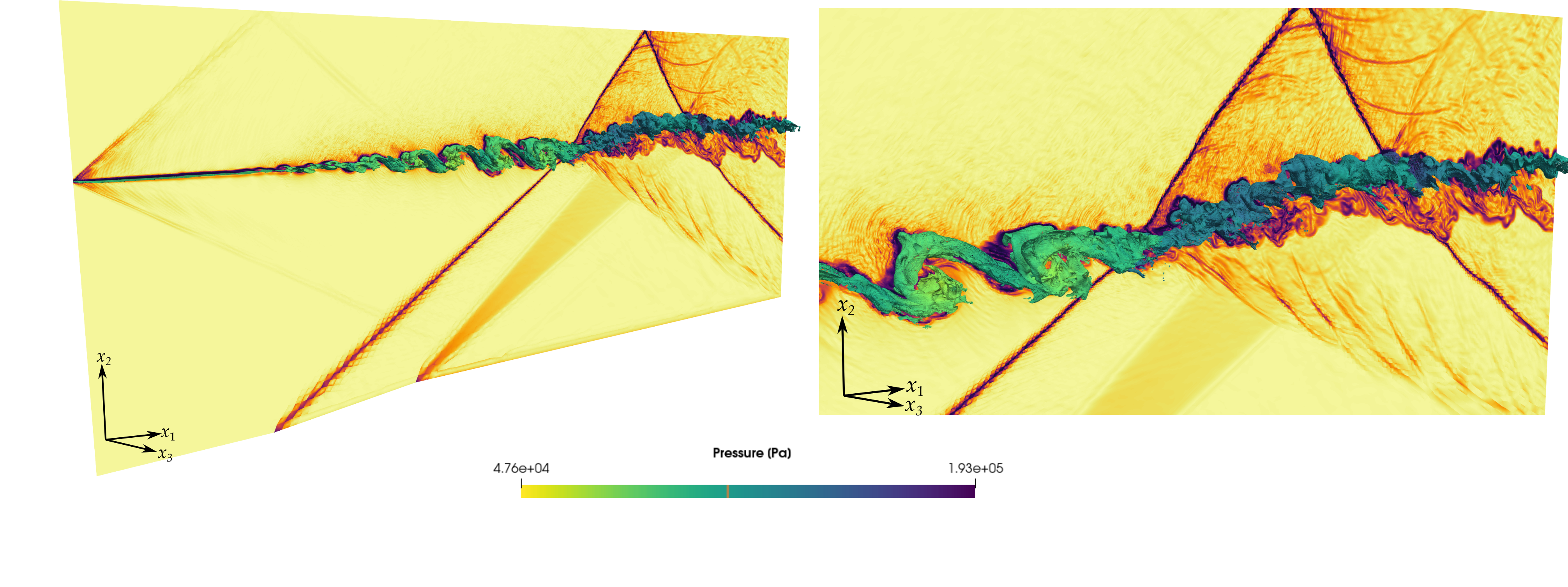
Figure 5.15: $Y_{OH}$ and numerical Schlieren results for three-dimensional shock/mixing-layer interaction. The unsteady inflow specification uses $(n_{1},n_{2},n_{3},n_{4})=(1,3,11,13)$, $(A_{1},A_{2},A_{3},A_{4})=(0.25\times 10^{-5},1.25\times 10^{-5},1.25\times 10^{-6},0.625\times 10^{-5})$ m, $B_{1}=1.25\times 10^{-5}$ m, $h_{t}$ = $2.5\times 10^{-5}$ m, $q_{1}=12$, and $(m_{0},m_{1},m_{2})=(8,4,16)$, . The length scale is chosen to be $L_{s}=0.00005$ m.

6 Concluding remarks

In this paper, we developed a fully conservative, positivity-preserving, and entropy-bounded DG formulation for the chemically reacting, compressible Navier-Stokes equations. The formulation builds on the fully conservative, positivity-preserving, and entropy-bounded DG formulation for the chemically reacting, compressible Euler equations that we previously introduced [10, 11]. A key ingredient is the positivity-preserving Lax-Friedrichs-type viscous flux function devised by Zhang [16] for the monocomponent case, which we extended to multicomponent flows with species diffusion in a manner that separates the inviscid and viscous fluxes. This is in contrast with the work by Du and Yang [17], who similarly extended said flux function, but treated the inviscid and viscous fluxes together. We discussed in detail the consideration of boundary conditions and the pressure-equilibrium-preserving techniques by Johnson and Kercher [2], introducing additional constraints on the time step size. Entropy boundedness is enforced on only the convective contribution since the minimum entropy principle only applies to the Euler equations [22, 23] and the viscous flux function is not fully compatible with said entropy bound. Drawing from [16], we proposed an adaptive solution procedure that favors large time step sizes and the BR2 viscous flux function since the Lax-Friedrichs-type viscous flux function was found to more likely lead to spurious oscillations. Small time step sizes and/or the Lax-Friedrichs-type viscous flux function are employed only when necessary. However, it should be noted that the Lax-Friedrichs-type viscous flux function guarantees a finite time-step size such that the positivity property is maintained. The proposed methodology is compatible with high-order polynomials and curved elements of arbitrary shape.

The DG methodology was applied to a series of test cases. The first two comprised smooth, one-dimensional flows: advection-diffusion of a thermal bubble and a premixed flame. In the former, optimal convergence was demonstrated for both viscous flux functions. In the latter, we obtained a much more accurate solution on a relatively coarse mesh with the proposed methodology than with conventional species clipping. Next, we computed viscous shock-tube flow and found that just as in the inviscid setting, enforcement of entropy boundedness considerably reduces the magnitude of large-scale instabilities that otherwise appear if only the positivity property is enforced. Finally, we computed two-dimensional, moving, viscous detonation waves and three-dimensional shock/mixing-layer interaction, demonstrating that the proposed formulation can accurately and robustly compute complex reacting flows with detailed chemistry using high-order polynomial approximations. Discrete conservation of mass and total energy was verified. Future work will entail the simulation of larger-scale viscous, chemically reacting flows involving more complex geometries.

Appendix A Boundary conditions

The boundary conditions here were originally described by Johnson and Kercher [2], building on the discussion in [33].

A.1 Supersonic inflow

Letting $y_{\infty}$ denote the fully prescribed state, we specify

$$y_{\partial}\left(y^{+},n^{+}\right)=y_{\infty} \textup{ on }\epsilon\qquad\forall\epsilon\in\mathcal{E}_{\mathrm{in}},$$

$$\mathcal{F}_{\partial,k}^{\nu}\left(y_{\partial}\left(y^{+},n^{+}\right),\nabla y^{+}\right)=\mathcal{F}_{k}^{\nu}\left(y_{\infty},\nabla y^{+}\right) \textup{ on }\epsilon\qquad\forall\epsilon\in\mathcal{E}_{\mathrm{in}},$$

$$\mathcal{F}_{\partial}^{c\dagger}\left(y^{+},n^{+}\right)=\mathcal{F}^{c}\left(y_{\infty}\right)\cdot n^{+} \textup{ on }\epsilon\qquad\forall\epsilon\in\mathcal{E}_{\mathrm{in}}.$$

A.2 Supersonic outflow

This boundary condition is given by

$$y_{\partial}\left(y^{+},n^{+}\right)=y^{+} \textup{ on }\epsilon\qquad\forall\epsilon\in\mathcal{E}_{\mathrm{out}},$$

$$\mathcal{F}_{\partial,k}^{\nu}\left(y_{\partial}\left(y^{+},n^{+}\right),\nabla y^{+}\right)=\mathcal{F}_{k}^{\nu}\left(y^{+},\nabla y^{+}\right) \textup{ on }\epsilon\qquad\forall\epsilon\in\mathcal{E}_{\mathrm{out}},$$

$$\mathcal{F}_{\partial}^{c\dagger}\left(y^{+},n^{+}\right)=\mathcal{F}^{c}\left(y^{+}\right)\cdot n^{+} \textup{ on }\epsilon\qquad\forall\epsilon\in\mathcal{E}_{\mathrm{out}},$$

where the boundary state is simply extrapolated from the interior.

A.3 Slip wall

We define the boundary velocity, $v_{\partial}=\left(v_{\partial,1},\ldots,v_{\partial,d}\right)$, as

$$v_{\partial}\left(y^{+},n^{+}\right)=\left(v_{1}^{+}-\left(\sum_{k=1}^{d}v_{k}^{+}n_{k}^{+}\right)n_{1}^{+},\cdots,v_{d}^{+}-\left(\sum_{k=1}^{d}v_{k}^{+}n_{k}^{+}\right)n_{d}^{+}\right).$$

We then have

$$y_{\partial}\left(y^{+},n^{+}\right)=\left(\rho^{+}v_{\partial,1},\ldots,\rho^{+}v_{\partial,d},\left(\rho e_{t}\right)^{+},C_{i}^{+},\ldots,C_{n_{s}}^{+}\right)^{T} \textup{ on }\epsilon\qquad\forall\epsilon\in\mathcal{E}_{\mathrm{slip}},$$

$$\mathcal{F}_{\partial,k}^{\nu}\left(y_{\partial}\left(y^{+},n^{+}\right),\nabla y^{+}\right)=\mathcal{F}_{k}^{\nu}\left(y_{\partial}\left(y^{+},n^{+}\right),\nabla y^{+}\right) \textup{ on }\epsilon\qquad\forall\epsilon\in\mathcal{E}_{\mathrm{slip}},$$

$$\mathcal{F}_{\partial}^{c\dagger}\left(y^{+},n^{+}\right)=\mathcal{F}^{c\dagger}\left(y^{+},2y_{\partial}\left(y^{+},n^{+}\right)-y^{+},n^{+}\right) \textup{ on }\epsilon\qquad\forall\epsilon\in\mathcal{E}_{\mathrm{slip}}.$$

The viscous boundary flux is obtained from the boundary state and the interior gradient.

A.4 Adiabatic wall

Here, let $v_{\partial}$ be a prescribed boundary velocity. This boundary condition is then given by

$$y_{\partial}\left(y^{+},n^{+}\right)=\left(\rho^{+}v_{\partial,1},\ldots,\rho^{+}v_{\partial,d},\left(\rho e_{t}\right)^{+},C_{i}^{+},\ldots,C_{n_{s}}^{+}\right)^{T} \textup{ on }\epsilon\qquad\forall\epsilon\in\mathcal{E}_{\mathrm{adi}},$$

$$\mathcal{F}_{\partial,k}^{\nu}\left(y_{\partial}\left(y^{+},n^{+}\right),\nabla y^{+}\right)=\begin{pmatrix}\frac{\partial\tau_{1k}}{\partial\left(\nabla y\right)}\left(y_{\partial}\right):\nabla y^{+}\\ \vdots\\ \frac{\partial\tau_{dk}}{\partial\left(\nabla y\right)}\left(y_{\partial}\right):\nabla y^{+}\\ {\textstyle\sum_{j=1}^{d}}v_{\partial,j}\frac{\partial\tau_{kj}}{\partial\left(\nabla y\right)}\left(y_{\partial}\right):\nabla y^{+}\\ 0\\ \vdots\\ 0\end{pmatrix} \textup{ on }\epsilon\qquad\forall\epsilon\in\mathcal{E}_{\mathrm{adi}},$$

$$\mathcal{F}_{\partial}^{c\dagger}\left(y^{+},n^{+}\right)=\mathcal{F}^{c}\left(y_{\partial}\left(y^{+},n^{+}\right)\right)\cdot n^{+} \textup{ on }\epsilon\qquad\forall\epsilon\in\mathcal{E}_{\mathrm{adi}},$$

where the species diffusion velocities and heat flux have been set to zero. The two boundary conditions below are not directly used in this study, but we include them for completeness.

A.5 Isothermal wall

Again, let $v_{\partial}$ be a prescribed boundary velocity. We specify

$$y_{\partial}\left(y^{+},n^{+}\right)=\left(\rho_{\partial}v_{\partial,1},\ldots,\rho_{\partial}v_{\partial,d},\rho_{\partial}u_{\partial}+0.5\cdot{\textstyle\sum_{j=1}^{d}}\rho_{\partial}v_{\partial,k}v_{\partial,k},C_{\partial,i},\ldots,C_{\partial,n_{s}}\right)^{T} \textup{ on }\epsilon\qquad\forall\epsilon\in\mathcal{E}_{\mathrm{iso}},$$

$$\mathcal{F}_{\partial,k}^{\nu}\left(y_{\partial}\left(y^{+},n^{+}\right),\nabla y^{+}\right)=\begin{pmatrix}\frac{\partial\tau_{1k}}{\partial\left(\nabla y\right)}\left(y_{\partial}\right):\nabla y^{+}\\ \vdots\\ \frac{\partial\tau_{dk}}{\partial\left(\nabla y\right)}\left(y_{\partial}\right):\nabla y^{+}\\ \left[{\textstyle\sum_{j=1}^{d}}v_{\partial,j}\frac{\partial\tau_{kj}}{\partial\left(\nabla y\right)}\left(y_{\partial}\right)-\frac{\partial q_{k}}{\partial\left(\nabla y\right)}\left(y_{\partial}\right)\right]:\nabla y^{+}\\ 0\\ \vdots\\ 0\end{pmatrix} \textup{ on }\epsilon\qquad\forall\epsilon\in\mathcal{E}_{\mathrm{iso}},$$

$$\mathcal{F}_{\partial}^{c\dagger}\left(y^{+},n^{+}\right)=\mathcal{F}^{c}\left(y_{\partial}\left(y^{+},n^{+}\right)\right)\cdot n^{+} \textup{ on }\epsilon\qquad\forall\epsilon\in\mathcal{E}_{\mathrm{iso}},$$

where $T_{\partial}$ is the prescribed boundary temperature, $C_{\partial,i}$ is the boundary concentration of the $i$th species,

$$C_{\partial,i}\left(y^{+}\right)=\frac{T^{+}}{T_{\partial}}C_{i}^{+}.$$

$\rho_{\partial}$ is the boundary density,

$$\rho_{\partial}=\sum_{i=1}^{n_{s}}W_{i}C_{\partial,i},$$

and $u_{\partial}$ is the boundary internal energy, which is evaluated at $T_{\partial}$.

A.6 Characteristic

Let $y^{*}\left(y^{+},y_{\infty},n^{+}\right)$ be the characteristic boundary value. Its derivation for non-reflecting inflow and outflow boundary conditions can be found in [2]. This boundary condition is then given as

$$y_{\partial}\left(y^{+},n^{+}\right)=y^{*}\left(y^{+},y_{\infty},n^{+}\right) \textup{ on }\epsilon\qquad\forall\epsilon\in\mathcal{E}_{\mathrm{cha}},$$

$$\mathcal{F}_{\partial,k}^{\nu}\left(y_{\partial}\left(y^{+},n^{+}\right),\nabla y^{+}\right)=\mathcal{F}_{k}^{\nu}\left(y_{\partial}\left(y^{+},n^{+}\right),\nabla y^{+}\right) \textup{ on }\epsilon\qquad\forall\epsilon\in\mathcal{E}_{\mathrm{cha}},$$

$$\mathcal{F}_{\partial}^{c\dagger}\left(y^{+},n^{+}\right)=\mathcal{F}^{c\dagger}\left(y^{+},y_{\partial}\left(y^{+},n^{+}\right),n^{+}\right) \textup{ on }\epsilon\qquad\forall\epsilon\in\mathcal{E}_{\mathrm{cha}}.$$

Appendix B Supporting lemma 

In the following, let $\Delta y$ denote the quantity

$$\Delta y=\left(\Delta(\rho v),\Delta(\rho e_{t}),\Delta C_{1},\ldots,\Delta C_{n_{s}}\right)^{T}.$$

The lemma below is related to that in [11, Appendix B].

Lemma 17.

Assume that $y=\left(\rho v,\rho e_{t},C\right)^{T}$ is in $\mathcal{G}$ and that $C_{i}>0,\>\forall i$. Then $\check{y}=y-\alpha^{-1}\Delta y$, where $\alpha>0$, is also in $\mathcal{G}$ under the following conditions:

$$\alpha>\alpha^{*}\left(y,\Delta y\right)=\left.\max\left\{\max_{i=1,\ldots,n_{s}}\frac{\Delta C_{i}}{C_{i}},\alpha_{T},0\right\}\right|_{\left(y,\Delta y\right)},$$ (B.1)

where

$$\alpha_{T}=\begin{cases}\frac{-\mathsf{b}+\sqrt{\mathsf{b}^{2}-4\rho^{2}u\mathsf{g}}}{2\rho^{2}u},&\mathsf{b}^{2}-4\rho^{2}u\mathsf{g}\geq 0\\ 0,&\mathrm{otherwise}\end{cases},$$ (B.2)

$\mathsf{b}=-\rho e_{t}\mathsf{M}-\rho\Delta(\rho e_{t})+\rho v\cdot\Delta(\rho v)+2\rho u_{0}\mathsf{M}$, $\mathsf{g}=\mathsf{M}\Delta(\rho e_{t})-\frac{1}{2}\left|\Delta(\rho v)\right|^{2}-u_{0}\mathsf{M}^{2}$, and $\mathsf{M}=\sum_{i=1}^{n_{s}}W_{i}\Delta C_{i}$.

Proof.

The proof is similar to that for Lemma 1. $\check{y}=y-\alpha^{-1}\Delta y$ can be expanded as

$$\begin{split}\check{y}=&\left(\check{\rho v},\check{\rho e_{t}},\check{C_{1}},\ldots,\check{C}_{n_{s}}\right)^{T}\\ =&\left(\rho v-\alpha\Delta(\rho v),\rho e_{t}-\alpha\Delta(\rho e_{t}),C_{1}-\alpha\Delta C_{1},\ldots,C_{n_{s}}-\alpha\Delta C_{n_{s}}\right)^{T}.\end{split}$$

$\check{C_{i}}=C_{i}-\alpha^{-1}\Delta C_{i}>0,\;\forall i$ under the condition

$$\alpha>\max\left\{\max_{i=1,\ldots,n_{s}}\frac{\Delta C_{i}}{C_{i}},0\right\}.$$

$Z\left(\check{y}\right)$, where $Z$ is defined as in Equation (4.7), can be expressed as

$$Z\left(y-\alpha^{-1}\Delta y\right)= \sum_{i=1}^{n_{s}}W_{i}\left(C_{i}-\alpha^{-1}\Delta C_{i}\right)\left(\rho e_{t}-\alpha^{-1}\Delta(\rho e_{t})\right)$$

$$-\frac{1}{2}\left|\rho v-\alpha^{-1}\Delta(\rho v)\right|^{2}-\left[\sum_{i=1}^{n_{s}}W_{i}\left(C_{i}-\alpha^{-1}\Delta C_{i}\right)\right]^{2}u_{0},$$

which, after multiplying both sides by $\alpha^{2}$, can be rewritten as

$$\alpha^{2}Z\left(y-\alpha^{-1}\Delta y\right)= \rho^{2}u\alpha^{2}-\mathsf{b}\alpha+\mathsf{g}.$$ (B.3)

Setting the RHS of Equation (B.3) equal to zero yields a quadratic equation with $\alpha$ as the unknown. Since $\rho^{2}u$ is positive, the quadratic equation is convex. As such, if $\mathsf{b}^{2}-4\rho^{2}u\mathsf{g}<0$, then no real roots exist, and $Z\left(y-\alpha^{-1}\Delta y\right)>0$ for all $\alpha\neq 0$; otherwise, at least one real root exists, in which case a sufficient condition to ensure $Z\left(y-\alpha^{-1}\Delta y\right)>0$ is $\alpha>\alpha_{0}$, where $\alpha_{0}$ is given by

$$\alpha_{0}=\max\left\{\frac{-\mathsf{b}+\sqrt{\mathsf{b}^{2}-4\rho^{2}u\mathsf{g}}}{2\rho^{2}u},0\right\}.$$

∎

References

- [1] K. Bando, M. Sekachev, M. Ihme, Comparison of algorithms for simulating multi-component reacting flows using high-order discontinuous Galerkin methods (2020). doi:10.2514/6.2020-1751.
- [2] R. F. Johnson, A. D. Kercher, A conservative discontinuous Galerkin discretization for the chemically reacting Navier–Stokes equations, Journal of Computational Physics 423 (2020) 109826. doi:10.1016/j.jcp.2020.109826.
- [3] R. Abgrall, Generalisation of the Roe scheme for the computation of mixture of perfect gases, La Recherche Aérospatiale 6 (1988) 31–43.
- [4] S. Karni, Multicomponent flow calculations by a consistent primitive algorithm, Journal of Computational Physics 112 (1) (1994) 31 – 43. doi:https://doi.org/10.1006/jcph.1994.1080.
- [5] R. Abgrall, How to prevent pressure oscillations in multicomponent flow calculations: A quasi conservative approach, Journal of Computational Physics 125 (1) (1996) 150 – 160. doi:https://doi.org/10.1006/jcph.1996.0085.
- [6] R. Abgrall, S. Karni, Computations of compressible multifluids, Journal of Computational Physics 169 (2) (2001) 594 – 623. doi:https://doi.org/10.1006/jcph.2000.6685.
- [7] Y. Lv, M. Ihme, Discontinuous Galerkin method for multicomponent chemically reacting flows and combustion, Journal of Computational Physics 270 (2014) 105 – 137. doi:https://doi.org/10.1016/j.jcp.2014.03.029.
- [8] G. Billet, J. Ryan, A Runge–Kutta discontinuous Galerkin approach to solve reactive flows: The hyperbolic operator, Journal of Computational Physics 230 (4) (2011) 1064 – 1083. doi:https://doi.org/10.1016/j.jcp.2010.10.025.
- [9] A. Gouasmi, K. Duraisamy, S. M. Murman, E. Tadmor, A minimum entropy principle in the compressible multicomponent Euler equations, ESAIM: Mathematical Modelling and Numerical Analysis 54 (2) (2020) 373–389.
- [10] E. J. Ching, R. F. Johnson, A. D. Kercher, Positivity-preserving and entropy-bounded discontinuous Galerkin method for the chemically reacting, compressible Euler equations. Part I: The one-dimensional case, arXiv preprint arXiv:2211.16254 https://arxiv.org/abs/2211.16254 (2022).
- [11] E. J. Ching, R. F. Johnson, A. D. Kercher, Positivity-preserving and entropy-bounded discontinuous Galerkin method for the chemically reacting, compressible Euler equations. Part II: The multidimensional case, arXiv preprint arXiv:2211.16297 https://arxiv.org/abs/2211.16297 (2022).
- [12] Y. Jiang, H. Liu, Invariant-region-preserving DG methods for multi-dimensional hyperbolic conservation law systems, with an application to compressible Euler equations, Journal of Computational Physics 373 (2018) 385–409.
- [13] X. Zhang, C.-W. Shu, On positivity-preserving high order discontinuous Galerkin schemes for compressible Euler equations on rectangular meshes, Journal of Computational Physics 229 (23) (2010) 8918–8934.
- [14] F. Bassi, S. Rebay, GMRES discontinuous Galerkin solution of the compressible Navier-Stokes equations, in: Discontinuous Galerkin Methods, Springer, 2000, pp. 197–208.
- [15] R. Hartmann, P. Houston, An optimal order interior penalty discontinuous Galerkin discretization of the compressible Navier–Stokes equations, Journal of Computational Physics 227 (22) (2008) 9670–9685.
- [16] X. Zhang, On positivity-preserving high order discontinuous Galerkin schemes for compressible Navier–Stokes equations, Journal of Computational Physics 328 (2017) 301–343.
- [17] J. Du, Y. Yang, High-order bound-preserving discontinuous Galerkin methods for multicomponent chemically reacting flows, Journal of Computational Physics 469 (2022) 111548.
- [18] J. Huang, C.-W. Shu, Bound-preserving modified exponential Runge–Kutta discontinuous Galerkin methods for scalar hyperbolic equations with stiff source terms, Journal of Computational Physics 361 (2018) 111–135.
- [19] J. Du, Y. Yang, Third-order conservative sign-preserving and steady-state-preserving time integrations and applications in stiff multispecies and multireaction detonations, Journal of Computational Physics 395 (2019) 489–510.
- [20] J. Du, C. Wang, C. Qian, Y. Yang, High-order bound-preserving discontinuous Galerkin methods for stiff multispecies detonation, SIAM Journal on Scientific Computing 41 (2) (2019) B250–B273.
- [21] T. Dzanic, F. D. Witherden, Positivity-preserving entropy-based adaptive filtering for discontinuous spectral element methods, Journal of Computational Physics 468 (2022) 111501.
- [22] E. Tadmor, A minimum entropy principle in the gas dynamics equations, Applied Numerical Mathematics 2 (3-5) (1986) 211–219.
- [23] J.-L. Guermond, B. Popov, Viscous regularization of the Euler equations and entropy principles, SIAM Journal on Applied Mathematics 74 (2) (2014) 284–305.
- [24] B. J. McBride, S. Gordon, M. A. Reno, Coefficients for calculating thermodynamic and transport properties of individual species (1993).
- [25] B. J. McBride, M. J. Zehe, S. Gordon, NASA Glenn coefficients for calculating thermodynamic properties of individual species (2002).
- [26] T. Coffee, J. Heimerl, Transport algorithms for premixed, laminar steady-state flames, Combustion and Flame 43 (1981) 273 – 289. doi:https://doi.org/10.1016/0010-2180(81)90027-4.
- [27] R. Houim, K. Kuo, A low-dissipation and time-accurate method for compressible multi-component flow with variable specific heat ratios, Journal of Computational Physics 230 (23) (2011) 8527 – 8553. doi:https://doi.org/10.1016/j.jcp.2011.07.031.
- [28] R. J. Kee, J. A. Miller, G. H. Evans, G. Dixon-Lewis, A computational model of the structure and extinction of strained, opposed flow, premixed methane-air flames, Symposium (International) on Combustion 22 (1) (1989) 1479 – 1494. doi:https://doi.org/10.1016/S0082-0784(89)80158-4.
- [29] R. J. Kee, M. E. Coltrin, P. Glarborg, Chemically reacting flow: Theory and practice, John Wiley & Sons, 2005.
-
[30]
D. G. Goodwin, H. K. Moffat, r. l. speth,
cantera: an object-oriented software toolkit
for chemical kinetics, thermodynamics, and transport processes, version
2.4.0 (2018).
doi:10.5281/zenodo.1174508.
URL http://www.cantera.org - [31] C. R. Wilke, A viscosity equation for gas mixtures, J. Chem. Phys 18 (1950) 517–519. doi:10.1063/1.1747673.
- [32] S. Mathur, P. K. Tondon, S. C. Saxena, Thermal conductivity of binary, ternary and quaternary mixtures of rare gases, Molecular Physics 12 (1967) 569–579. doi:10.1080/00268976700100731.
- [33] R. Hartmann, T. Leicht, Higher order and adaptive DG methods for compressible flows, in: H. Deconinck (Ed.), VKI LS 2014-03: 37th Advanced VKI CFD Lecture Series: Recent developments in higher order methods and industrial application in aeronautics, Dec. 9-12, 2013, Von Karman Institute for Fluid Dynamics, Rhode Saint Genèse, Belgium, 2014.
- [34] D. Arnold, F. Brezzi, B. Cockburn, L. Marini, Unified analysis of discontinuous Galerkin methods for elliptic problems, SIAM Journal on Numerical Analysis 39 (5) (2002) 1749–1779.
- [35] E. Toro, Riemann solvers and numerical methods for fluid dynamics: A practical introduction, Springer Science & Business Media, 2013.
- [36] G. Strang, On the construction and comparison of difference schemes, SIAM Journal on Numerical Analysis 5 (3) (1968) 506–517.
- [37] S. Gottlieb, C. Shu, E. Tadmor, Strong stability-preserving high-order time discretization methods, SIAM review 43 (1) (2001) 89–112.
- [38] R. Spiteri, S. Ruuth, A new class of optimal high-order strong-stability-preserving time discretization methods, SIAM Journal on Numerical Analysis 40 (2) (2002) 469–491.
- [39] H. Atkins, C. Shu, Quadrature-free implementation of discontinuous Galerkin methods for hyperbolic equations, ICASE Report 96-51, 1996, Tech. rep., NASA Langley Research Center, nASA-CR-201594 (August 1996).
- [40] H. L. Atkins, C.-W. Shu, Quadrature-free implementation of discontinuous Galerkin method for hyperbolic equations, AIAA Journal 36 (5) (1998) 775–782.
- [41] Y. Lv, M. Ihme, Entropy-bounded discontinuous Galerkin scheme for Euler equations, Journal of Computational Physics 295 (2015) 715–739.
- [42] K. Wu, Minimum principle on specific entropy and high-order accurate invariant region preserving numerical methods for relativistic hydrodynamics, arXiv preprint arXiv:2102.03801 (2021).
- [43] E. Ching, Y. Lv, P. Gnoffo, M. Barnhardt, M. Ihme, Shock capturing for discontinuous Galerkin methods with application to predicting heat transfer in hypersonic flows, Journal of Computational Physics 376 (2019) 54–75.
- [44] J. Huang, C.-W. Shu, Positivity-preserving time discretizations for production–destruction equations with applications to non-equilibrium flows, Journal of Scientific Computing 78 (3) (2019) 1811–1839.
- [45] V. Giovangigli, Multicomponent flow modeling, Birkhauser, Boston, 1999.
- [46] A. Gouasmi, K. Duraisamy, S. M. Murman, Formulation of entropy-stable schemes for the multicomponent compressible Euler equations, Computer Methods in Applied Mechanics and Engineering 363 (2020) 112912.
- [47] X. Zhang, C.-W. Shu, A minimum entropy principle of high order schemes for gas dynamics equations, Numerische Mathematik 121 (3) (2012) 545–563.
- [48] C. Wang, X. Zhang, C.-W. Shu, J. Ning, Robust high order discontinuous Galerkin schemes for two-dimensional gaseous detonations, Journal of Computational Physics 231 (2) (2012) 653–665.
- [49] B. A. Wingate, M. A. Taylor, Performance of numerically computed quadrature points, Applied numerical mathematics 58 (7) (2008) 1030–1041.
- [50] A. Corrigan, A. Kercher, J. Liu, K. Kailasanath, Jet noise simulation using a higher-order discontinuous Galerkin method, in: 2018 AIAA SciTech Forum, 2018, AIAA-2018-1247.
- [51] C. K. Westbrook, Chemical kinetics of hydrocarbon oxidation in gaseous detonations, Combustion and Flame 46 (1982) 191 – 210. doi:https://doi.org/10.1016/0010-2180(82)90015-3.
- [52] E. S. Oran, E. I. Weber J. W.and Stefaniw, M. H. Lefebvre, J. D. Anderson, A numerical study of a two-dimensional h2-o2-ar detonation using a detailed chemical reaction model, Combustion and Flame 113 (1) (1998) 147 – 163. doi:https://doi.org/10.1016/S0010-2180(97)00218-6.
- [53] M. H. Lefebvre, J. Weber, J. W., E. S. Oran, Proceedings of the IUTAM Symposium (B. Deshaies and L. F. da Silva, eds.) (30) (1998) 347 – 358.
- [54] C. Geuzaine, J.-F. Remacle, Gmsh: a three-dimensional finite element mesh generator with built-in pre- and post-processing facilities, International Journal for Numerical Methods in Engineering (79(11)) (2009) 1310–1331.
- [55] S. K. Burrows, R. F. Johnson, E. J. Ching, Development of a model verification test case for chemically reacting flows: Mixing layer interacting with an impinging oblique shock, Tech. Rep. NRL/6041/MR–2022/2, U.S. Naval Research Laboratory (October 2022).
- [56] P. J. M. Ferrer, R. Buttay, G. Lehnasch, A. Mura, A detailed verification procedure for compressible reactive multicomponent navier–stokes solvers, Computers & Fluids 89 (2014) 88–110. doi:https://doi.org/10.1016/j.compfluid.2013.10.014.