Test Bench Study on Attitude Estimation
in Ground Effect Region Based on Motor Current
for In-Flight Inductive Power Transfer of Drones

Abstract

To overcome the short flight duration of drones, research on in-flight inductive power transfer has been recognized as an essential solution. Thus, it is important to accurately estimate and control the attitude of the drones which operate close to the charging surface. To this end, this paper proposes an attitude estimation method based solely on the motor current for precision flight control in the ground effect region. The model for the estimation is derived based on the motor equation when it rotates at a constant rotational speed. The proposed method is verified on the simulations and experiments. It allows simultaneous estimation of altitude and pitch angle with the accuracy of 0.30 m and 0.04 rad, respectively. The minimum transmission efficiency of the in-flight power transfer system based on the proposed estimation is calculated as 95.3 %, which is sufficient for the efficient system.

I Introduction

Drones have been increasingly utilized in many aspects of human society. There are many promising applications where the drones have to operate in the desirable route. A typical application is security surveillance with the mission schematic shown in Fig. 1. In the diagram, charging the battery every lap is needed, which deteriorates the drone’s operating rate. To realize the continuous monitoring capability, a lot of drones are required; however, this increases system cost a lot to assign enough drones to complete the mission.

Although much research has been conducted to extend the flight duration, an inductive power transfer for flying drones [1, 2] is the most effective way to increase the operating rate in fixed route operations. The diagram of the in-flight inductive power transfer system is shown in Fig. 2. In this system, the drones fly near the transfer coils placed on the roof or wall, and they are wirelessly powered while monitoring the area.

This system makes it challenging to avoid power deviation and efficiency deterioration because drones fly along the transmitter coils while fluctuating, as shown in Fig. 2. Previous studies realize the constant power transfer by controlling the converters [3, 4]. However, they assumed that the mutual inductance fluctuates, so does not consider improving efficiency just by suppressing the mutual inductance deviation.

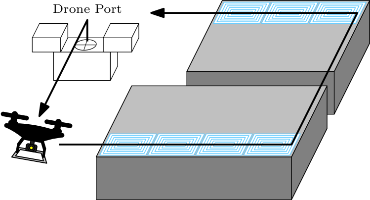
Figure 1: Security mission with in-flight inductive power transfer.

Figure 2: Deterioration of the coupling coefficient $k$ without precise attitude control on in-flight inductive power transfer system.

To maintain the stability and high efficiency of in-flight power transfer, it is essential to precisely estimate and control both the altitude and attitude of the drone body. This would be great challenge due to the existence of the ground effect (GE), which happens as the drones fly closely to the transmitting coils. As a basic study toward in-flight power transfer for drones, the focus of this paper is to develop suitable estimation algorithm. Although the ultrasonic sensor has sufficient ability for altitude measurement near the ground, angle measurement is not precise enough for advanced motion control[5]. For more precise estimation, the sensor fusion mainly combined with the inertial measurement unit (IMU) is utilized[6]. In [7], Svacha et al. focused on the motor speed as the additional information for the proposed model-based sensor fusion to enhance the performance; however, the GE was not addressed by the aforementioned studies.

With respect to the above discussion, this paper shows that by properly addressing the GE, the motor current can be effectively utilized to estimate the drone attitude via a model-based algorithm. Previous researches only mentioned the infinite model between the motor current and the altitude in the GE region, which shows no current is flowing when the altitude is zero. This paper proposes a new finite motor current model which can show a non-zero current in the GE region based on [8, 9, 10], which discusses the finite thrust model in the GE region. The model is identified experimentally. Then, attitude estimation with the proposed model is validated in the simulations and experiments.

The reminder of this paper is organized as follows. In section $\mathrm{II}$, the proposed model for attitude estimation from the motor equation is proposed. In section $\mathrm{III}$, the proposed method is verified in the simulations. In section $\mathrm{IV}$, the proposed method is verified in the experiments. In section $\mathrm{V}$, the conclusion is shown, and future studies are mentioned.

II Modeling and proposed attitude estimation

In this section, the attitude estimation method with the motor current model is proposed. First, previous studies about the in-GE motor power and thrust force model are introduced. Second, a motor current model for the GE region is proposed based on the motor equation and finite thrust model, and the attitude estimation relation for the altitude and the pitch angle is derived from the proposed motor current model. Finally, the test bench dynamics is explained for the simulations and experimental evaluation of the proposed method.

II-A Previous studies about motor power and thrust force model in GE region

In 1937, Betz proposed in [11] that the ratio of in-GE motor power to out-GE motor power is expressed as

$$\left[\frac{P}{P_{\infty}}\right]_{F=\mathrm{const.}}=\frac{2z}{R},$$ (1)

where $P$, $P_{\infty}$, $z$, and $R$ are the power of the drone, out-GE motor power of the drone, altitude of the propeller, and the propeller radius, respectively. This equation is only correct when $z\ll R$. In 1955, Cheeseman and Bennett proposed another expression of the aforementioned ratio in [12] as

$$\left[\frac{P}{P_{\infty}}\right]_{F=\mathrm{const.}}=\frac{1}{1+\left(\frac{R}{4z}\right)^{2}}.$$ (2)

The above equation is derived from aerodynamic theories, such as blade element theory (BET). In 1976, Hayden proposed in [13] that the ratio is expressed as

$$\left[\frac{P}{P_{\infty}}\right]_{F=\mathrm{const.}}=\frac{1}{A+B\left(\frac{2R}{z}\right)^{2}},$$ (3)

where $A$ and $B$ are the function coefficients, respectively, which are determined experimentally. These models assume that the required power is zero on the ground. However, this assumption is not suitable to describe the drone motion at the ground level. Even if the altitude is zero, the drones need the thrust force to fly. Consequently, a certain power is required to rotate the propeller. The in-GE motor current model, which shows a non-zero value on the ground, is needed to estimate attitude from the model precisely. Unfortunately, no model has been proposed to satisfy such purpose.

The same situations occurred in the field for the modeling of in-GE thrust; the estimated thrust value surges with the previous in-GE thrust model, so many researchers tackled the finite thrust model.

In that situation, the finite in-GE thrust model is proposed in [8, 9, 10] by He et al. as

$$\left[\frac{F}{F_{\infty}}\right]_{P=\text{ const. }}=1+C_{a}e^{-C_{b}z/R},$$ (4)

where the maximum ratio of thrust $C_{a}$ is calculated as

$$C_{a}=\frac{\sqrt{192C_{l_{\alpha}}\sigma\theta_{0}+9C_{l_{\alpha}}\sigma^{2}}-3C_{l_{\alpha}}\sigma}{32\theta_{0}+3C_{l_{\alpha}}\sigma-\sqrt{192C_{l_{\alpha}}\sigma\theta_{0}+9C_{l_{\alpha}}\sigma^{2}}},$$ (5)

where $C_{l_{\alpha}}$, $\sigma$, and $\theta_{0}$ are the lift coefficient, solidity of the propeller, and collective pitch angle of the propeller, respectively. $C_{b}$ shows the profile of the in-GE induced velocity. It can be calculated based on aerodynamic theories, such as BET. In the paper, $C_{a}$ is calculated from the propeller geometry, and $C_{b}$ is experimentally determined. In this paper, the model parameters are experimentally validated. Using this finite model, the in-GE motor current model, which shows a non-zero value on the ground, is derived in the next part.

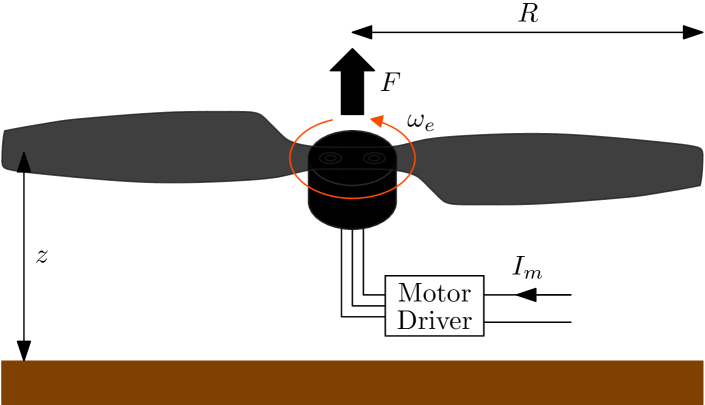
Figure 3: Propeller operational diagram in ground region.

II-B Proposed finite motor current model with respect to ground effect region

In this part, the finite motor current model is derived, assuming the constant battery voltage. The motor equation is written as

$$J_{\omega}\frac{\mathrm{d}\omega}{\mathrm{d}t}+D_{\omega}\omega={K_{\tau}}I_{m}-C_{Q}\omega^{2}-T_{C},$$ (6)

where $J_{\omega}$, $D_{\omega}$, $\omega$, $K_{\tau}$, $I_{m}$, $C_{Q}$, and $T_{C}$ are the motor inertia, motor viscosity, rotational speed, torque coefficient, motor current, counter torque coefficient, and coulomb torque, respectively. When the motor is operating at the constant rotational speed $\omega_{c}$, the below equations are established:

$${K_{\tau}}I_{m} =C_{Q}\omega_{c}^{2}+D_{\omega}\omega_{c}+T_{C}\approx C_{Q}\omega_{c}^{2},$$

$$\therefore\hskip 8.53581ptI_{m} =\frac{C_{Q}}{K_{\tau}}\omega_{c}^{2}.$$ (7)

The approximation is validated because $D_{\omega}\omega_{c},T_{C}\ll C_{Q}\omega_{c}^{2}$.

When the drone is flying out-GE region, the thrust force needed for the flight $F$ is equal to the calculated output of the propeller force $F_{e}$ ($F=F_{e}$). Based on BET when the propeller rotational speed is $\omega_{e}$, the thrust force is expressed as

$$F_{e}=C_{F}\omega_{e}^{2},$$ (8)

where $C_{F}$ is the thrust coefficient. From 7,

$$I_{m_{\infty}}=\frac{C_{Q}}{K_{\tau}}\omega_{e}^{2}$$ (9)

is derived, where $I_{m_{\infty}}$ is the out-GE motor current. From 8 and 9 and $F=F_{e}$,

$$I_{m_{\infty}}=\frac{C_{Q}}{K_{\tau}C_{F}}F$$ (10)

is calculated.

When the drone is flying in the GE region,

$$F=C_{IGE}F_{e}$$ (11)

is derived, where $C_{IGE}$ is the in-GE thrust coefficient, and it is written as below based on 4 in this paper:

$$C_{IGE}=1+C_{a}e^{-C_{b}z/R}.$$ (12)

From 7, 8, and 11,

$$I_{m}=\frac{C_{Q}}{K_{\tau}C_{F}}\cdot\frac{F}{C_{IGE}}$$ (13)

is calculated. Finally, from 10 and 13,

$$\left[\frac{I_{m}}{I_{m_{\infty}}}\right]_{F=\text{ const. }}=\frac{1}{C_{IGE}}=\frac{1}{1+C_{a}e^{-C_{b}z/R}}$$ (14)

is derived. The coefficient of 14 is experimentally identified for each propeller as shown in Fig. 4. The identified values are shown in Table. I. The direct current component of the measured motor current is extracted by Fourier fast transform, and the coefficients are adjusted by least squares method.

From 14, the altitude at the propeller is expressed with the motor current as

$$z=g(I_{m})=-\frac{R}{C_{b}}\log\left\{\frac{1}{C_{a}}\left(\left[\frac{I_{m_{\infty}}}{I_{m}}\right]_{F=\text{ const. }}-1\right)\right\}.$$ (15)

In this paper, the proposed attitude estimation method is implemented for the bench system of two-degree-of-freedom drone as shown in Fig. 5. Based on 15, each propeller altitude $z_{1}$ and $z_{2}$ is calculated, and the altitude of the gravitational point $z$ and the pitch angle $\theta$ as shown in Fig. 5 are estimated as

$$z=\frac{z_{1}+z_{2}}{2},\hskip 14.22636pt\theta=h\left(z_{1},z_{2}\right)=\arcsin{\left(\frac{z_{1}-z_{2}}{2l}\right)}.$$ (16)

In the experiments, nonlinear recursive least squares (RLS) [14] is implemented to prevent the estimation deterioration due to the fluctuation of the measured motor current.

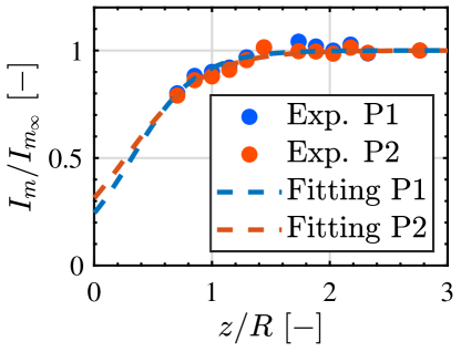
Figure 4: Identification result of the proposed motor current model.

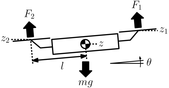
Figure 5: Two-degree-of-freedom drone model.

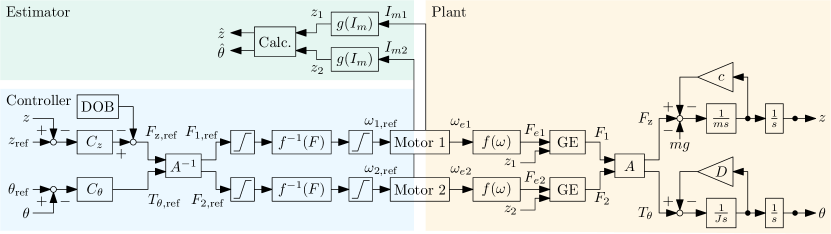
Figure 6: Block diagram of simulation system.

II-C Test bench dynamics

The motion of the bench system in Fig. 5 is described by the following equations:

$$m\frac{\mathrm{d}^{2}z}{\mathrm{d}t^{2}}+c\frac{\mathrm{d}z}{\mathrm{d}t} =F_{1}\cos{\theta}+F_{2}\cos{\theta}-mg=F_{z}-mg,$$ (17a)

$$J\frac{\mathrm{d}^{2}\theta}{\mathrm{d}t^{2}}+D\frac{\mathrm{d}\theta}{\mathrm{d}t} =F_{1}l-F_{2}l=T_{\theta},$$ (17b)

where $F_{1}$, $F_{2}$, $F_{z}$, $T_{\theta}$, $m$, $c$, $J$, $D$, $l$, and $g$ are the thrust force of propeller 1, thrust force of propeller 2, total thrust force affecting the body in parallel to the gravitational force, total torque affecting the body, total mass of the body, motor, and propeller, drag coefficient of the body, inertia of the body, rotational viscosity of the body, pitch moment arm, and gravitational constant, respectively. Besides, the below relations between $F_{1}$, $F_{2}$ and $F_{z}$, $T_{\theta}$ are established:

$$\left[\begin{array}[]{l}F_{z}\\ T_{\theta}\end{array}\right] =\left[\begin{array}[]{cc}\cos\theta&\cos\theta\\ l&-l\end{array}\right]\left[\begin{array}[]{l}F_{1}\\ F_{2}\end{array}\right]=A^{-1}\left[\begin{array}[]{l}F_{1}\\ F_{2}\end{array}\right],$$ (18i)

$$\left[\begin{array}[]{l}F_{1}\\ F_{2}\end{array}\right] =\left[\begin{array}[]{cc}\frac{1}{2\cos{\theta}}&\frac{1}{2l}\\ \frac{1}{2\cos{\theta}}&-\frac{1}{2l}\end{array}\right]\left[\begin{array}[]{l}F_{z}\\ T_{\theta}\end{array}\right]=A\left[\begin{array}[]{l}F_{z}\\ T_{\theta}\end{array}\right].$$ (18r)

Based on 17, the nominal plant of the vertical motion and pitch motion can be defined as

$$G_{z}=\frac{1}{ms^{2}},\hskip 14.22636ptG_{J}=\frac{1}{Js^{2}}.$$ (19)

These nominal plants are utilized to design the controllers in the next section.

III Simulations

Simulations are conducted to verify the proposed method. First, the simulation system is introduced based on the block diagram as shown in Fig. 6. Second, attitude estimation with the proposed model is conducted in simulations.

In Fig. 6, $z_{\mathrm{ref}}$, $\theta_{\mathrm{ref}}$, $T_{z\mathrm{,ref}}$, $T_{\theta\mathrm{,ref}}$, $T_{1\mathrm{,ref}}$, $T_{2\mathrm{,ref}}$, $\omega_{1\mathrm{,ref}}$,and $\omega_{2\mathrm{,ref}}$ show the reference value of the altitude at the center of gravity (COG), pitch angle, thrust at the COG, moment around the COG, thrust at propeller 1, thrust at propeller 2, angular velocity at propeller 1, and angular velocity at propeller 2, respectively. $z$ and $\theta$ show the measured value of the altitude at the COG, and pitch angle, respectively. $\omega_{e1}$, $\omega_{e2}$, $F_{e1}$, and $F_{e2}$ show the rotational speed of propeller 1, rotational speed of propeller 2, thrust without GE at propeller 1, and thrust without GE at propeller 2, respectively. Function $f(\omega)$ is expressed as 8 and $f^{-1}(F)$ is expressed as the inverse of 8. The GE is implemented as 4. $C_{z}$ and $C_{\theta}$ are designed as a PID and PD controller based on 19, respectively. Each controller is designed by multiple root pole placement, and each pole are set at $10\text{\,}\mathrm{r}\mathrm{a}\mathrm{d}\mathrm{/}\mathrm{s}$ and $30\text{\,}\mathrm{r}\mathrm{a}\mathrm{d}\mathrm{/}\mathrm{s}$, respectively. The motor model is implemented based on [15]. The disturbance observer (DOB) is implemented for the altitude controller because the viscosity is large in the experimental bench system[16]. Other parameters in Fig. 6 are shown in Table. I.

TABLE I: Simulation prameters.

Parameter	Value
Torque Coefficient 1 $K_{\tau 1}$	$66.4\text{\,}\mathrm{m}\mathrm{N}\mathrm{m}\mathrm{/}\mathrm{A}$
Torque Coefficient 2 $K_{\tau 2}$	$65.1\text{\,}\mathrm{m}\mathrm{N}\mathrm{m}\mathrm{/}\mathrm{A}$
Inertia of Motor with Propeller 1 $J_{\omega 1}$	$0.4\text{\,}\mathrm{k}\mathrm{g}\mathrm{m}^{2}$
Inertia of Motor with Propeller 2 $J_{\omega 2}$	$0.392\text{\,}\mathrm{k}\mathrm{g}\mathrm{m}^{2}$
Motor Viscosity 1 $D_{\omega 1}$	$4.6\text{\,}\mathrm{\SIUnitSymbolMicro}\mathrm{m}\mathrm{s}\mathrm{/}\mathrm{r}\mathrm{a}\mathrm{d}$
Motor Viscosity 2 $D_{\omega 2}$	$4.51\text{\,}\mathrm{\SIUnitSymbolMicro}\mathrm{m}\mathrm{s}\mathrm{/}\mathrm{r}\mathrm{a}\mathrm{d}$
Counter Torque Coefficient 1 $C_{{Q1}}$	$9.56\text{\,}\mathrm{\SIUnitSymbolMicro}\mathrm{N}\mathrm{m}\mathrm{s}^{2}\mathrm{/}\mathrm{r}\mathrm{a}\mathrm{d}^{2}$
Counter Torque Coefficient 2 $C_{{Q2}}$	$9.88\text{\,}\mathrm{\SIUnitSymbolMicro}\mathrm{N}\mathrm{m}\mathrm{s}^{2}\mathrm{/}\mathrm{r}\mathrm{a}\mathrm{d}^{2}$
Coulomb Torque 1 $T_{{C1}}$	$2.4\text{\,}\mathrm{m}\mathrm{N}\mathrm{m}$
Coulomb Torque 2 $T_{{C2}}$	$2.35\text{\,}\mathrm{m}\mathrm{N}\mathrm{m}$
Total Mass of Body, Motor, and Propeller $m$	$7.0\text{\,}\mathrm{kg}$
Drag Coefficient of Body $c$	$1.0\text{\,}\mathrm{m}\mathrm{N}\mathrm{s}\mathrm{/}\mathrm{m}$
Inertia of Body $J$	$2.34\text{\,}\mathrm{k}\mathrm{g}\mathrm{m}^{2}$
Rotational Viscosity of Body $D$	$0.1\text{\,}\mathrm{\SIUnitSymbolMicro}\mathrm{N}\mathrm{m}\mathrm{s}\mathrm{/}\mathrm{r}\mathrm{a}\mathrm{d}$
Pitch Moment Arm $l$	$0.63\text{\,}\mathrm{m}$
Rotor Radius $R$	$0.34\text{\,}\mathrm{m}$
Thrust Coefficient $C_{F}$	$0.399\text{\,}\mathrm{m}\mathrm{N}\mathrm{s}^{2}\mathrm{/}\mathrm{r}\mathrm{a}\mathrm{d}^{2}$
Ground Effect Coefficient 1 $C_{{a\mathrm{P1}}}$ / $C_{{a\mathrm{P2}}}$	$3.11$ / $2.20$
Ground Effect Coefficient 2 $C_{{b\mathrm{P1}}}$ / $C_{{b\mathrm{P2}}}$	$3.56$ / $2.97$

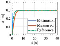
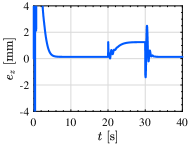
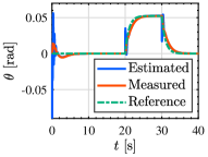
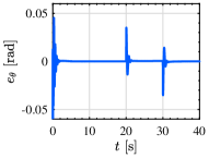
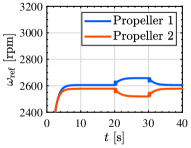
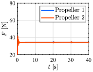
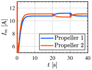
Figure 7: Simulation results of altitude and pitch angle estimation. (a) Altitude $z$ (b) Altitude estimation error $e_{z}$ (c) Pitch angle $\theta$ (d) Pitch Angle estimation error $e_{\theta}$ (e) Angular velocity of motor $\omega$ (f) Thrust $F$ (g) Motor current $I_{m}$

Simulation results to verify the attitude estimation method with the proposed model are shown in Fig. 7. The simulations are conducted assuming in-flight inductive power transfer system. In the simulations, the drone starts to fly at $0\text{\,}\mathrm{s}$ and hovers at $0.3\text{\,}\mathrm{m}$ height which is in the GE region. At $20\text{\,}\mathrm{s}$, the pitch angle rises to $0.05\text{\,}\mathrm{r}\mathrm{a}\mathrm{d}$, which demonstrates the forward flight, and goes down to $0.0\text{\,}\mathrm{r}\mathrm{a}\mathrm{d}$ while maintaining the same height. In this condition, the distance between the transfer coil and receiver coil is assumed to be $0.1\text{\,}\mathrm{m}$, and the coupling coefficient of the system, which means that the coupling strength between the transfer coil and receiver coil is assumed to be 0.10, which is the reasonable value for the efficient inductive power transfer.

Figs. 7 and 7 show the altitude responses. In the state condition, the maximum error of the altitude estimation is below $3\text{\,}\mathrm{m}\mathrm{m}$, which is sufficient for the efficient in-flight inductive power transfer. Figs. 7 and 7 show the pitch angle responses. In the state condition, the maximum error of the pitch angle estimation is below $0.04\text{\,}\mathrm{r}\mathrm{a}\mathrm{d}$, which is also sufficient to the in-flight inductive power transfer. Figs. 7, 7, and 7 show the motor rotational speed response, thrust response, and motor current response, respectively. In these figures, it is observed that the differences are increased when the reference value of the pitch angle is non-zero. It can be seen that the state values in Figs. 7, 7, and 7 do not coincide because the motor parameters are not the same in the simulations. However, the differences are normalized with the out-GE motor current $I_{m_{\infty}}$ shown in Fig. 4 Therefore, the motor parameters deviations do not affect the estimation performance in the simulations.

The simulation results with model parameter errors and the same reference input of the attitude are shown in Table. II. The estimation errors and root mean square deviation (RMSD) are shown in Table. II. $C_{an}$ and $C_{bn}$ are the nominal model parameters. It is assumed that the nominal parameters deviate from the actual coefficients $C_{a}$ and $C_{b}$. From Table. II, it is observed that the maximum errors of the altitude and the pitch angle are $23\text{\,}\mathrm{m}\mathrm{m}$ and $\pm 0.04\text{\,}\mathrm{r}\mathrm{a}\mathrm{d}\mathrm{/}\mathrm{s}$.

TABLE II: Evaluation results of parameter errors.

	Altitude error / RMSD	Pitch angle error / RMSD
Without Model Errors	$2\text{\,}\mathrm{m}\mathrm{m}$ / $10\text{\,}\mathrm{m}\mathrm{m}$	$\pm 0.04\text{\,}\mathrm{r}\mathrm{a}\mathrm{d}$ / $6.79\text{\,}\mathrm{m}\mathrm{r}\mathrm{a}\mathrm{d}$
$C_{an}=1.05C_{a},C_{bn}=1.05C_{b}$	$-10\text{\,}\mathrm{m}\mathrm{m}$ / $12.9\text{\,}\mathrm{m}\mathrm{m}$	$\pm 0.04\text{\,}\mathrm{r}\mathrm{a}\mathrm{d}$ / $6.69\text{\,}\mathrm{m}\mathrm{r}\mathrm{a}\mathrm{d}$
$C_{an}=1.05C_{a},C_{bn}=0.95C_{b}$	$23\text{\,}\mathrm{m}\mathrm{m}$ / $24.1\text{\,}\mathrm{m}\mathrm{m}$	$\pm 0.04\text{\,}\mathrm{r}\mathrm{a}\mathrm{d}$ / $7.30\text{\,}\mathrm{m}\mathrm{r}\mathrm{a}\mathrm{d}$
$C_{an}=0.95C_{a},C_{bn}=1.05C_{b}$	$-20\text{\,}\mathrm{m}\mathrm{m}$ / $20.6\text{\,}\mathrm{m}\mathrm{m}$	$\pm 0.04\text{\,}\mathrm{r}\mathrm{a}\mathrm{d}$ / $6.49\text{\,}\mathrm{m}\mathrm{r}\mathrm{a}\mathrm{d}$
$C_{an}=0.95C_{a},C_{bn}=0.95C_{b}$	$12\text{\,}\mathrm{m}\mathrm{m}$ / $14.2\text{\,}\mathrm{m}\mathrm{m}$	$\pm 0.04\text{\,}\mathrm{r}\mathrm{a}\mathrm{d}$ / $7.39\text{\,}\mathrm{m}\mathrm{r}\mathrm{a}\mathrm{d}$

IV Experiments

In this section, the experimental validation is conducted in the bench system as shown in Fig. 8. The bench system consists of the two propellers, linear encoder, rotational encoder, controller, and power supply. The controller for the bench system is the same for the simulations as shown in Fig. 6.

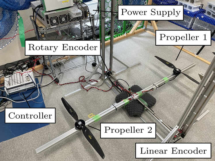
Figure 8: Drone bench system for experimental validation.

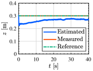
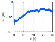
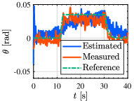
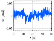
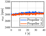
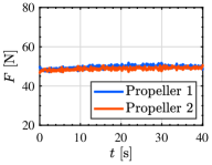
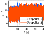
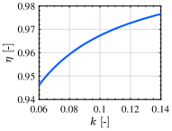
Figure 9: Experimental results for altitude and pitch angle estimation. (a) Altitude $z$ (b) Altitude estimation error $e_{z}$ (c) Pitch angle $\theta$ (d) Pitch Angle estimation error $e_{\theta}$ (e) Angular velocity of motor $\omega$ (f) Thrust $F$ (g) Motor current $I_{m}$ (h) Transmission efficiency of the inductive power transfer system at $\omega=$85\text{\,}\mathrm{k}\mathrm{H}\mathrm{z}$$, $R_{1}=$108\text{\,}\mathrm{m}\Omega$$, $R_{2}=$32.5\text{\,}\mathrm{m}\Omega$$, $L_{1}=$236\text{\,}\mathrm{\SIUnitSymbolMicro}\mathrm{H}$$, $L_{2}=$18.9\text{\,}\mathrm{\SIUnitSymbolMicro}\mathrm{H}$$ on the resonance condition $\eta$

Experimental results are shown in Fig. 9. Figs. 9, 9, and 9 show the reference value of the motor rotational speed, thrust, and motor current, respectively. There exist signal fluctuations due to motor vibration and sensor noises.

Figs. 9 and 9 show the altitude responses. The estimations are conducted based on the fluctuating motor currents shown in Fig. 9, so nonlinear RLS mentioned before is implemented. Its forgetting factor is 0.9985 for each propeller. From Fig. 9, the state maximum error of the altitude estimation from the measured altitude value is $-0.03\text{\,}\mathrm{m}$ and RMSD of the error is $0.0391\text{\,}\mathrm{m}$. When the drone flies at $0.30\text{\,}\mathrm{m}$, the coupling coefficient $k$ and the transmission efficiency of the inductive power transfer system $\eta$ as shown in Fig. 9 is 0.10 and $96.7\text{\,}\mathrm{\char 37\relax}$, respectively. If there is an altitude deviation of $0.03\text{\,}\mathrm{m}$, the coupling coefficient varies between 0.07 and 0.13[17]. This deviation of the coupling coefficient leads to the deviation of the transmission efficiency from $95.3\text{\,}\mathrm{\char 37\relax}$ to $97.5\text{\,}\mathrm{\char 37\relax}$, which is sufficient for the efficient inductive power transfer. As shown above, the estimation has the enough performance for the efficient inductive power transfer. Fig. 9 and Fig. 9 show the pitch angle responses. In the state condition, the maximum error of the pitch angle estimation is below $0.04\text{\,}\mathrm{r}\mathrm{a}\mathrm{d}$ and RMSD of the error is $0.0130\text{\,}\mathrm{r}\mathrm{a}\mathrm{d}$, which is also sufficient for the in-flight inductive power transfer.

V Conclusion

In this paper, we proposed a novel motor current model based on the motor equation at the constant rotational speed and finite thrust model. It is shown that the proposed model can fit the measured results, and estimation performance of the model is validated with the simulations and experiments. The estimation errors are $0.30\text{\,}\mathrm{m}$ maximum with respect to the altitude, and $0.04\text{\,}\mathrm{r}\mathrm{a}\mathrm{d}$ maximum with respect to the pitch angle in the experiments. These estimation errors might lead to the efficiency deviation from $95.3\text{\,}\mathrm{\char 37\relax}$ to $97.5\text{\,}\mathrm{\char 37\relax}$, which is enough for the efficient inductive power transfer.

In the future, the proposed method will be extended by considering the fusion of the current sensor with the other motion sensors, such as the IMU, ultrasonic sensor, and on-board vision system. In parallel, the robustness of the proposed method for the model parameter errors is investigated. The estimated attitude will be applied for the precise flight control scheme on the in-flight inductive power transfer system. The demonstration of the in-flight inductive power transfer with a real vehicle is also conducted as the demonstration of the precise flight control near the ground.

References

- [1] K. Chen and Z. Zhang, “In-Flight Wireless Charging: A Promising Application-Oriented Charging Technique for Drones,” IEEE Industrial Electronics Magazine (Early Access), pp. 2–12, 2023.
- [2] J. M. Arteaga, S. Aldhaher, G. Kkelis, C. Kwan, D. C. Yates, and P. D. Mitcheson, “Dynamic Capabilities of Multi-MHz Inductive Power Transfer Systems Demonstrated With Batteryless Drones,” IEEE Transactions on Power Electronics, vol. 34, no. 6, pp. 5093–5104, 2019.
- [3] Z. Zhang, S. Shen, Z. Liang, S. H. K. Eder, and R. Kennel, “Dynamic-Balancing Robust Current Control for Wireless Drone-in-Flight Charging,” IEEE Transactions on Power Electronics, vol. 37, no. 3, pp. 3626–3635, 2022.
- [4] Y. Gu, J. Wang, Z. Liang, and Z. Zhang, “Mutual-Inductance-Dynamic-Predicted Constant Current Control of LCC-P Compensation Network for Drone Wireless In-Flight Charging,” IEEE Transactions on Industrial Electronics, vol. 69, no. 12, pp. 12 710–12 719, 2022.
- [5] V. Chandrasegar and J. Koh, “Estimation of Azimuth Angle Using an Ultrasonic Sensor for Automobile,” Remote Sensing, vol. 15, no. 7, pp. 1–14, 2023.
- [6] C. Li, S. Wang, Y. Zhuang, and F. Yan, “Deep Sensor Fusion Between 2D Laser Scanner and IMU for Mobile Robot Localization,” IEEE Sensors Journal, vol. 21, no. 6, pp. 8501–8509, 2021.
- [7] J. Svacha, G. Loianno, and V. Kumar, “Inertial Yaw-Independent velocity and attitude estimation for High-Speed quadrotor flight,” IEEE Robotics and Automation Letters, vol. 4, no. 2, pp. 1109–1116, 2019.
- [8] X. He, M. Calaf, and K. K. Leang, “Modeling and Adaptive Nonlinear Disturbance Observer for Closed-Loop Control of In-Ground-Effects on Multi-Rotor UAVs,” in ASME 2017 Dynamic Systems and Control Conference, 2017.
- [9] X. He, G. Kou, M. Calaf, and K. K. Leang, “In-Ground-Effect Modeling and Nonlinear-Disturbance Observer for Multirotor Unmanned Aerial Vehicle Control,” Journal of dynamic systems, measurement, and control, vol. 141, no. 7, pp. 071 013–1–071 013–11, 2019.
- [10] X. He and K. K. Leang, “Quasi-Steady In-Ground-Effect Model for Single and Multirotor Aerial Vehicles,” AIAA Journal, vol. 58, no. 12, pp. 5318–5331, 2020.
- [11] A. Betz, “The Ground Effect on Lifting Propellers,” Tech. Rep. NACA-TM-836, 1937.
- [12] I. C. Cheeseman and W. E. Bennett, “The Effect of the Ground on a Helicopter Rotor in Forward Flight,” Tech. Rep., 1955.
- [13] J. S. Hayden, “The Effect of the Ground on Helicopter Hovering Power Required,” in AHS 32nd annual forum, 1976.
- [14] M. Umayahara, Y. Iiguni, and H. Maeda, “A Nonlinear Recursive Least Squares Algorithm for Crosstalk-Resistant Noise Canceler,” Electronics and Communications in Japan. Part 3, Fundamental Electronic Science, vol. 86, no. 5, pp. 36–44, 2003.
- [15] Y. Naoki, S. Nagai, and H. Fujimoto, “Mode-switching algorithm to improve variable-pitch-propeller thrust generation for drones under motor current limitation,” IEEE/ASME Transactions on Mechatronics, vol. 28, no. 4, pp. 2003–2011, 2023.
- [16] B.-M. Nguyen, T. Kobayashi, K. Sekitani, M. Kawanishi, and T. Narikiyo, “Altitude Control of Quadcopters with Absolute Stability Analysis,” IEEJ Journal of Industry Applications, vol. 11, no. 4, pp. 562–572, 2022.
- [17] K. Fujimoto, K. Yokota, S. Nagai, and H. Fujimoto, “Modeling and Verification of Pitch-Dependent Coupling Coefficient for WPT to Flying Drone,” in 2021 IEE-Japan Industry Applications Society Conference (JIASC), 2021.