Blow-up Sets of Ricci Curvatures of
Complete Conformal Metrics

Abstract.

A version of the singular Yamabe problem in smooth domains in a closed manifold yields complete conformal metrics with negative constant scalar curvatures. In this paper, we study the blow-up phenomena of Ricci curvatures of these metrics on domains whose boundary is close to a certain limit set of a lower dimension. We will characterize the blow-up set according to the Yamabe invariant of the underlying manifold. In particular, we will prove that all points in the lower dimension part of the limit set belong to the blow-up set on manifolds not conformally equivalent to the standard sphere and that all but one point in the lower dimension part of the limit set belong to the blow-up set on manifolds conformally equivalent to the standard sphere. In certain cases, the blow-up set can be the entire manifold. We will demonstrate by examples that these results are optimal.

1. Introduction

A version of the singular Yamabe problem in bounded domains in the compact manifold can be formulated as follows. Given a compact Riemannian manifold $(M,g)$ of dimension $n\geq 3$ without boundary and a smooth submanifold $\Gamma$ in $M$, does there exist a complete conformal metric on $M\setminus\Gamma$ with a negative constant scalar curvature $-n(n-1)$? For $(M,g)=(S^{n},g_{S^{n}})$, Loewner and Nirenberg [22] proved that there exists a complete conformal metric on $S^{n}\setminus\Gamma$ with the constant scalar curvature $-n(n-1)$ if and only if dim$(\Gamma)>(n-2)/2$. Aviles and McOwen [4] proved a similar result for the general compact manifold $(M,g)$. As a consequence, we can take the dimension of the submanifold to be $n-1$ and conclude the following result. In any compact Riemannian manifold with a smooth boundary, there exists a complete conformal metric with a negative constant scalar curvature $-n(n-1)$. Such a metric is referred to as a singular Yamabe metric in this paper.

The singular Yamabe metrics in smooth domains can be viewed as generalizations of the Poincaré metric in the unit ball in Euclidean space, and have sectional curvatures asymptotically equal to $-1$ near the boundary. It is natural to investigate whether they have negative sectional curvatures or negative Ricci curvatures in the entire domain, or whether their Ricci curvatures can be controlled in a uniform way. Conditions on a bound or a lower bound of Ricci curvatures are widely used in geometry and analysis on manifolds. For example, they play an important role in Yau’s gradient estimate for harmonic function [26], Li-Yau’s heat kernel estimates [26], Bishop-Gromov’s volume growth estimates [25], Gromov’s precompactness theorem for a family of manifolds [25], Cheeger-Colding theory[6], and Cheeger-Colding-Tian [7], to name a few.

There are many works concerning the singular Yamabe metrics. Andersson, Chruściel, and Friedrich [1] and Mazzeo [24] established polyhomogeneous expansions for conformal factors of the singular Yamabe metrics. Graham [10] studied volume renormalizations for singular Yamabe metrics and characterized the coefficient of the first logarithmic terms in the expansions for conformal factors of the singular Yamabe metrics by a variation of the coefficients of the first logarithmic terms in the volume expansions. Gursky and the first author [11], and Chen, Lai, and Wang [8] studied Escobar’s Yamabe compactifications for Poincaré-Einstein manifolds by using the polyhomogeneous expansions of the singular Yamabe metrics. In [30], the second and third authors obtained rigidity and gap results for boundary integrals of the global coefficient when $n=2$. Recently, Li [19] recovered the existence of the singular Yamabe metric on compact manifolds with boundary through flow method. Chang, McKeown, and Yang [5] studied the scattering problem for the singular Yamabe metrics and applied the results to the study of the conformal geometry of compact manifolds with boundary.

In [15], the first two authors studied the negativity of Ricci curvatures of the singular Yamabe metrics and investigated whether these metrics have negative sectional curvatures or negative Ricci curvatures. They proved that these metrics indeed have negative Ricci curvatures in bounded convex domains in the Euclidean space. They also provided general constructions of domains in compact manifolds and demonstrated that the negativity of Ricci curvatures does not hold if the boundary is close to certain sets of low dimensions. For singular Yamabe metrics, Ricci curvatures are uniformly bounded from below if and only if they are uniformly bounded since the scalar curvature of these complete conformal metrics is assumed to be a fixed negative constant.

In this paper, we study the blow-up phenomena of Ricci curvatures of the singular Yamabe metrics. In particular, we characterize the blow-up sets and use the blow-up sets to obtain some information of the conformal geometry of underlying manifold. Our setting is similar to that in [15] and will appear repeatedly. It is convenient to formulate the following assumption.

Assumption 1.1.

Let $(M,g)$ be a compact Riemannian manifold of dimension $n\geq 3$ without boundary and $\Gamma\subset M$ be a nonempty compact set. Suppose that $\Omega_{i}$ is a sequence of increasing smooth domains in $M\setminus\Gamma$, which converges to $M\setminus\Gamma$, and that $g_{i}$ is the complete conformal metric in $\Omega_{i}$ with a constant scalar curvature $-n(n-1)$ as in [4].

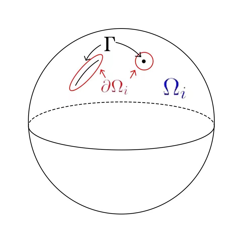
Figure 1. $\Omega_{i}\rightarrow M\setminus\Gamma$

By the convergence of $\Omega_{i}$ to $M\setminus\Gamma$, we mean $\cup_{i=1}^{\infty}\Omega_{i}=M\setminus\Gamma$ and, for any $\varepsilon>0$, $\partial\Omega_{i}$ is in the $\varepsilon$-neighborhood of $\Gamma$ for all large $i$. By smooth domains, we always mean domains with smooth boundaries. In [15], the first two authors proved that the maximal Ricci curvature of $g_{i}$ in $\Omega_{i}$ diverges to $\infty$ as $i\to\infty$, under appropriate assumptions on $(M,g)$ and $\Gamma$. In particular, $\Gamma$ is required to be a disjoint union of finitely many closed smooth embedded submanifolds in $M$ of varying dimensions, between $0$ and $(n-2)/2$.

In the following, we refer to the compact set $\Gamma$ as the limit set. With $\Gamma$, $\{\Omega_{i}\}$, and $\{g_{i}\}$ as in Assumption 1.1, we define the associated blow-up set by

$$\mathcal{B}_{\Gamma,\{\Omega_{i}\}}=\big{\{}x\in M; \,\lim_{m\to\infty}\sup_{i}|Ric_{g_{i}}(x_{m})|=\infty$$

$$\text{ for some sequence }\{x_{m}\}\subset M\setminus\Gamma\text{ with }x_{m}\rightarrow x\big{\}}.$$

In other words, the blow-up set $\mathcal{B}_{\Gamma,\{\Omega_{i}\}}$ consists of the limits of sequences of points where the maximal Ricci components of $g_{i}$ diverges to $\infty$. It is obvious that the blow-up set $\mathcal{B}_{\Gamma,\{\Omega_{i}\}}$ is a closed set of $M$. As we will see, the blow-up set $\mathcal{B}_{\Gamma,\{\Omega_{i}\}}$ depends on the limit set $\Gamma$ as well as the exhausting domains $\{\Omega_{i}\}$. For a fixed compact set $\Gamma$ in $(S^{n},g_{S^{n}})$, different sets of exhausting domains may yield different blow-up sets.

In this paper, we aim to characterize the blow-up set $\mathcal{B}_{\Gamma,\{\Omega_{i}\}}$. First, we assume that the limit $\Gamma$ consists of three components as follows:

(1.1) $$\begin{split}&\text{$\Gamma_{1}$ is a compact subset in $M$ of Hausdorff dimension less than $(n-2)/2$},\\ &\text{$\Gamma_{2}$ is a closed subset in the union of countably many closed $C^{1}$-embedded}\\ &\qquad\text{submanifolds in $M$ of dimension $(n-2)/2$},\end{split}$$

and

(1.2) $$\begin{split}&\text{$\Gamma_{3}$ is a disjoint union of finitely many closed smooth embedded}\\ &\qquad\text{ submanifolds in $M$ of varying dimensions greater than $(n-2)/2$}.\end{split}$$

We point out that the lower dimensional component $\Gamma_{1}$ is allowed to have non-integer dimensions. Even if it has an integer dimension, it is not necessarily a smooth submanifold. We also point out that $\Gamma$ is allowed have a higher dimensional component $\Gamma_{3}$. We emphasize that $\Gamma_{2}$ is assumed to be a closed set itself.

We will prove the following two results. The higher dimensional part $\Gamma_{3}$ of the limit set $\Gamma$ is present in the first result and is absent in the second result.

Theorem 1.2.

Let $(M,g)$, $\Gamma$, and $\{\Omega_{i}\}$ be as in Assumption 1.1, and $\Gamma=\Gamma_{1}\bigcup\Gamma_{2}\bigcup\Gamma_{3}$, for $\Gamma_{1},\Gamma_{2}$, and $\Gamma_{3}$ as in (1.1) and (1.2), with $(\Gamma_{1}\bigcup\Gamma_{2})\bigcap\Gamma_{3}=\emptyset$, $\Gamma_{1}\bigcup\Gamma_{2}\neq\emptyset$, and $\Gamma_{3}\neq\emptyset$. Then, $\Gamma_{1}\bigcup\Gamma_{2}\subseteq\mathcal{B}_{\Gamma,\{\Omega_{i}\}}\subseteq\Gamma$.

Theorem 1.3.

Let $(M,g)$, $\Gamma$, and $\{\Omega_{i}\}$ be as in Assumption 1.1, $\lambda(M,[g])$ be the Yamabe invariant of $(M,g)$, and $\Gamma=\Gamma_{1}\bigcup\Gamma_{2}$, for $\Gamma_{1}$ and $\Gamma_{2}$ as in (1.1).

$\mathrm{(1)}$ If $\lambda(M,[g])<0$, then $\mathcal{B}_{\Gamma,\{\Omega_{i}\}}=\Gamma$.

$\mathrm{(2)}$ If $\lambda(M,[g])=0$, then

$$\mathcal{B}_{\Gamma,\{\Omega_{i}\}}=\Gamma\bigcup\text{clos}\{x\in M:\,Ric_{\bar{g}}(x)\neq 0\text{ for some }\bar{g}\in[g]\text{ with }R_{\bar{g}}=0\},$$

where $R_{\bar{g}}$ is the scalar curvature of $\bar{g}$.

$\mathrm{(3)}$ If $\lambda(M,[g])>0$ and $(M,g)$ is not conformally equivalent to $S^{n}$, then $\Gamma\subseteq\mathcal{B}_{\Gamma,\{\Omega_{i}\}}$. If, in addition, $M$ is locally conformally flat, then $\mathcal{B}_{\Gamma,\{\Omega_{i}\}}=M$.

$\mathrm{(4)}$ If $(M,g)$ is conformally equivalent to $S^{n}$, then either $\Gamma\subseteq\mathcal{B}_{\Gamma,\{\Omega_{i}\}}$ or $\Gamma\setminus\{p\}\subseteq\mathcal{B}_{\Gamma,\{\Omega_{i}\}}$ for some isolated point $p\in\Gamma$.

We point out that the second component in the union in (2) is a well-defined closed set since any two conformal metrics of $g$ on $M$ with zero scalar curvatures differ from each other by a positive constant factor under the assumption $\lambda(M,[g])=0$.

As we see in Theorem 1.3, the Yamabe invariant plays an essential role in characterizing the blow-up sets. We now make several comments. First, (1)-(3) illustrate that the limit set $\Gamma$ is always contained in the blow-up set if $(M,g)$ is not conformally equivalent to $S^{n}$. Second, we will prove that all accumulation points of $\Gamma$ are always in the blow-up set. The difference between (3) and (4) lies on the number of isolated points in the limit set $\Gamma$ where blow-up occurs. On manifolds not conformally equivalent to the standard sphere, all isolated points in the limit set are in the blow-up set. While on manifolds conformally equivalent to the standard sphere, all but possibly one isolated point are in the blow-up set. Third, the blow-up sets may contain points outside the limit sets $\Gamma$, and maybe the entire manifold, as the second part of (3) demonstrates.

We will construct examples to demonstrate that Theorem 1.3(4) is optimal. For example, for the case $(M,g)=(S^{n},g_{S^{n}})$ and $\Gamma=\{p,q\}$ for two distinct points $p,q\in S^{n}$, with different sequences of exhausting domains, the blow-up set can be any one of $p$ and $q$, or $\{p,q\}$, or even the entire $S^{n}$. For the case $(M,g)=(S^{n},g_{S^{n}})$ and $\Gamma=\{p\}$ for a single point $p\in S^{n}$, with different sequences of exhausting domains, the blow-up set can be empty or nonempty. In general, the blow-up set can be quite complex if the Yamabe invariant is positive.

The proofs of Theorems 1.2-1.3 rely on a careful analysis of the Ricci curvatures of the complete conformal metrics near the boundary. The Yamabe invariant of $(M,g)$ and the higher dimensional part $\Gamma_{3}$ play crucial roles and determine behaviors of the convergence of the conformal factors. As in [15], when the underlying manifold has a positive Yamabe invariant, we need the positive mass theorem to study behaviors of conformal factors near isolated points in the limit set.

As consequences of Theorem 1.3, we have the following rigidity results. Under certain conditions, if Ricci curvatures of a sequence of singular Yamabe metrics remain bounded in a fixed small region, then the underlying manifold is conformally equivalent to the standard sphere equipped with the standard spherical metric.

Theorem 1.4.

Let $(M,g)$, $\Gamma$, $\{\Omega_{i}\}$, and $\{g_{i}\}$ be as in Assumption 1.1, and $\Gamma=\Gamma_{1}\bigcup\Gamma_{2}$ for $\Gamma_{1}$ and $\Gamma_{2}$ as in (1.1), with an isolated point $x_{0}$ in $\Gamma$. Suppose that the metric $g_{i}$ has uniformly bounded Ricci curvatures near $x_{0}$. Then, $M$ is conformally equivalent to the standard sphere $S^{n}$.

Theorem 1.5.

Let $(M,g)$, $\Gamma$, $\{\Omega_{i}\}$, and $\{g_{i}\}$ be as in Assumption 1.1, $M$ be locally conformally flat with $\lambda(M,[g])>0$, $\Gamma=\Gamma_{1}\bigcup\Gamma_{2}$ for $\Gamma_{1}$ and $\Gamma_{2}$ as in (1.1), and $x_{0}$ be any point in $M$. Suppose that the metric $g_{i}$ has uniformly bounded Ricci curvatures near $x_{0}$. Then, $M$ is conformally equivalent to the standard sphere $S^{n}$.

The paper is organized as follows. In Section 2, we discuss some preliminary identities and present two important lemmas concerning conformal factors. In Section 3, we prove Theorem 1.2 and Theorem 1.3(1)-(2). We also prove that all accumulation points of the limit set $\Gamma$ are in the blow-up sets. In Section 4, we discuss isolated points of $\Gamma$ and prove the first assertion in Theorem 1.3(3) and Theorem 1.3(4). In Section 5, we study whether blow-up sets contain points outside the limit sets and prove the second assertion in Theorem 1.3(3). In Section 6, we present several examples in $S^{n}$ to demonstrate the complexity of blow-up sets.

We would like to thank Matthew Gursky, Marcus Khuri, and Yuguang Shi for helpful discussions.

2. Preliminaries

In this section, we collect some basic results concerning the singular Yamabe metrics. We also prove two important convergence results concerning the conformal factors of the singular Yamabe metrics.

Let $(M,g)$ be a smooth compact Riemannian manifold of dimension $n\geq 3$ without boundary. The Yamabe invariant of $(M,g)$ is given by

$$\lambda(M,[g])=\inf\Big{\{}\frac{\int_{M}(|\nabla_{g}\phi|^{2}+\frac{n-2}{4(n-1)}S_{g}\phi^{2})dV_{g}}{(\int_{M}\phi^{\frac{2n}{n-2}}dV_{g})^{\frac{n-2}{n}}};\,\phi\in C^{\infty}(M),\phi>0\Big{\}}.$$

We define the conformal Laplacian of $(M,g)$ by

$$L_{g}=-\Delta_{g}+\frac{n-2}{4(n-1)}S_{g}.$$

For any functions $u$ and $\psi$ in $M$ with $\psi>0$, we have

(2.1) $$L_{g}(\psi u)=\psi^{\frac{n+2}{n-2}}L_{\psi^{\frac{4}{n-2}}g}(u).$$

Assume $\Omega\subset M$ is a smooth domain, with an $(n-1)$-dimensional boundary. We consider the following problem:

(2.2) $$\Delta_{g}u-\frac{n-2}{4(n-1)}S_{g}u =\frac{1}{4}n(n-2)u^{\frac{n+2}{n-2}}\quad\text{in }\,\Omega,$$

(2.3) $$u =\infty\quad\text{on }\partial\Omega,$$

where $S_{g}$ is the scalar curvature of $M$. According to Loewner and Nirenberg [22] for $(M,g)=(S^{n},g_{S^{n}})$ and Aviles and McOwen [4] for the general case, (2.2) and (2.3) admit a unique positive solution. The singular Yamabe metric $u^{\frac{4}{n-2}}g$ is a complete metric with a constant scalar curvature $-n(n-1)$ on $\Omega$.

Concerning boundary behaviors of the conformal factors, Andersson, Chruściel, and Friedrich [1] and Mazzeo [24] established the polyhomogeneous expansions. For the first several terms, we have

$$u=d^{-\frac{n-2}{2}}\Big{[}1+\frac{n-2}{4(n-1)}H_{\partial\Omega}d+O(d^{2})\Big{]},$$

where $d$ is the distance to $\partial\Omega$ and $H_{\partial\Omega}$ is the mean curvature of $\partial\Omega$ with respect to the interior unit normal vector of $\partial\Omega$.

Set

$$v=u^{-\frac{2}{n-2}}.$$

Then,

(2.4) $$v\Delta_{g}v+\frac{1}{2(n-1)}S_{g}v^{2} =\frac{n}{2}(|\nabla_{g}v|^{2}-1)\quad\text{in }\Omega,$$

(2.5) $$v =0\quad\text{on }\partial\Omega.$$

Moreover,

(2.6) $$v=d-\frac{1}{2(n-1)}H_{\partial\Omega}d^{2}+O(d^{3}).$$

This implies

(2.7) $$|\nabla_{g}v|=1\quad\text{on }\partial\Omega.$$

Consider the conformal metric

$$g_{\Omega}=u^{\frac{4}{n-2}}g=v^{-2}g.$$

For a unit vector $X$ with respect to $g$, $vX$ is a unit vector with respect to $g_{\Omega}$. Let $R_{ij}$ be the Ricci components of $g$ in a local frame for the metric $g$ and $R^{\Omega}_{ij}$ be the Ricci components of $g_{\Omega}$ in the corresponding frame for the metric $g_{\Omega}$. Then,

(2.8) $${R}^{\Omega}_{kl}=v^{2}R_{kl}+(n-2)\big{[}vv_{,kl}-\frac{1}{2}g_{kl}|\nabla_{g}v|^{2}\big{]}+g_{kl}\big{[}v\Delta_{g}v-\frac{n}{2}|\nabla_{g}v|^{2}\big{]}.$$

By (2.4), we have

(2.9) $${R}^{\Omega}_{kl}=v^{2}R_{kl}-\frac{1}{2(n-1)}v^{2}g_{kl}S_{g}+(n-2)\big{[}vv_{,kl}-\frac{1}{2}g_{kl}|\nabla_{g}v|^{2}\big{]}-\frac{n}{2}g_{kl}.$$

We now present two convergence results which generalize Lemma 4.1 in [15]. They play an important role in this paper.

Lemma 2.1.

Let $(M,g)$, $\Gamma$, and $\{\Omega_{i}\}$ be as in Assumption 1.1, and $\Gamma=\Gamma_{1}\bigcup\Gamma_{2}$ for $\Gamma_{1}$ and $\Gamma_{2}$ as in (1.1). Suppose that the scalar curvature $S_{g}$ is constant and that $u_{i}$ is the solution of (2.2) and (2.3) in $\Omega_{i}$. Then, for any positive integer $m$, if $S_{g}\geq 0$,

(2.10) $$u_{i}\rightarrow 0\quad\text{in }C^{m}_{\mathrm{loc}}(M\setminus\Gamma)\text{ as }i\rightarrow\infty,$$

and, if $S_{g}<0$,

(2.11) $$u_{i}\rightarrow\Big{(}\frac{-S_{g}}{n(n-1)}\Big{)}^{\frac{n-2}{4}}\quad\text{in }C^{m}_{\mathrm{loc}}(M\setminus\Gamma)\text{ as }i\rightarrow\infty.$$

Proof.

Recall that $\Gamma_{1}$ is a compact set in $M$ of Hausdorff dimension less than $(n-2)/2$ and $\Gamma_{2}$ is a closed subset in the union $\bigcup_{l=1}^{\infty}N_{l}$, where each $N_{l}$ is a closed $C^{1}$-embedded submanifold in $M$ of dimension $(n-2)/2.$

As in the proof of Lemma 4.1 in [15], we have $u_{i}\geq u_{i+1}$ in $\Omega_{i}$. It is straightforward to verify, for any $m$,

$$u_{i}\rightarrow u\quad\text{in }C^{m}_{\mathrm{loc}}(M\setminus\Gamma)\text{ as }i\rightarrow\infty,$$

where $u$ is a nonnegative solution of (2.2) in $M\setminus\Gamma$. We consider two cases.

Special Case. We first assume $\Gamma_{2}=\bigcup_{l=1}^{k}N_{l}$, where $k$ is a finite integer. Moreover, $\Gamma_{1}$ and $N_{l}$ are disjoint.

By Theorem 2.1 and Theorem 2.2 in [2], $u$ can be extended to the whole manifold $M$ and (2.2) holds in $M.$ Then,

(2.12) $$-\int_{M}|\nabla_{g}u|^{2}dV_{g}=\int_{M}\Big{(}\frac{n-2}{4(n-1)}S_{g}u^{2}+\frac{1}{4}n(n-2)u^{\frac{2n}{n-2}}\Big{)}dV_{g}.$$

If $S_{g}\geq 0$, then $u=0$ in $M$. If $S_{g}<0$, by the proof of Lemma 4.1 in [15], we have

$$u_{i}\geq\Big{(}\frac{-S_{g}}{n(n-1)}\Big{)}^{\frac{n-2}{4}}\quad\text{in }\Omega_{i}.$$

Hence,

$$u\geq\Big{(}\frac{-S_{g}}{n(n-1)}\Big{)}^{\frac{n-2}{4}}\quad\text{in }M.$$

Combining with (2.12), we have $u=\Big{(}\frac{-S_{g}}{n(n-1)}\Big{)}^{\frac{n-2}{4}}$ in $M$.

General Case. We now consider the general case. For unification, we write $N_{0}=\Gamma_{1}$. For each $l\geq 0$, let $\Omega_{i}^{l}$ be a sequence of increasing smooth domains in $M\setminus N_{l}$, which converges to $M\setminus N_{l}$, and $u_{i}^{l}$ be the solution of (2.2) and (2.3) in $\Omega_{i}^{l}$.

First, we consider $S_{g}\geq 0$. Take a fixed point $p\in M\setminus\overline{\cup_{l=0}^{\infty}N_{l}}$, and we will prove $u(p)=0$. Then, we have $u=0$ in $M\setminus\Gamma$. As in the special case, for any fixed $l\geq 0$, we have $u_{i}^{l}\rightarrow 0$ uniformly in any compact subsets of $M\setminus N_{l}$ as $i\rightarrow\infty$. Then, for any $\epsilon>0$, there exists an integer $i(l,\epsilon)$ such that $u_{i(l,\epsilon)}^{l}(p)<\epsilon/2^{l+1}$. Note that both $\Gamma_{1}$ and $\Gamma_{2}$ are closed and $\bigcup_{l=0}^{\infty}M\setminus\overline{\Omega_{i(l,\epsilon)}^{l}}$ covers $\Gamma_{1}\bigcup\Gamma_{2}$. Then, $\Gamma_{1}\bigcup\Gamma_{2}$ has a finite subcover, given by $M\setminus\overline{\Omega_{i(0,\epsilon)}^{0}}$, $M\setminus\overline{\Omega_{i(l_{1},\epsilon)}^{l_{1}}}$, $\cdots$, $M\setminus\overline{\Omega_{i(l_{k},\epsilon)}^{l_{k}}}$. It is easy to verify $u_{i(0,\epsilon)}^{0}+\sum_{j=1}^{k}u_{i(l_{j},\epsilon)}^{l_{j}}$ is a supersolution of (2.2) in $\Omega_{i(0,\epsilon)}^{0}\bigcap\big{(}\bigcap_{j=1}^{k}\Omega_{i(l_{j},\epsilon)}^{l_{j}}\big{)}$. Then by the maximum principle, we have $u(p)<\epsilon$. Hence, $u(p)=0$.

Next, we consider $S_{g}<0$. Without loss of generality, we assume $S_{g}=-n(n-1)$. Take a fixed point $p\in M\setminus\overline{\cup_{l=0}^{\infty}N_{l}}$, and we will prove $u(p)=1$. Then, we have $u=1$ in $M\setminus\Gamma$. By the special case, for any fixed $l\geq 0$, we have $u_{i}^{l}\geq 1$ and $u_{i}^{l}\rightarrow 1$ uniformly in any compact subsets of $M\setminus N_{l}$, as $i\rightarrow\infty$. Then, for any $\epsilon>0$, there exists an integer $i(l,\epsilon)$ such that $u_{i(l,\epsilon)}^{l}(p)<1+\epsilon/2^{l+1}$. Note that both $\Gamma_{1}$ and $\Gamma_{2}$ are closed and $\bigcup_{l=0}^{\infty}M\setminus\overline{\Omega_{i(l,\epsilon)}^{l}}$ covers $\Gamma_{1}\bigcup\Gamma_{2}$. Then, $\Gamma_{1}\bigcup\Gamma_{2}$ has a finite subcover, given by $M\setminus\overline{\Omega_{i(0,\epsilon)}^{0}}$, $M\setminus\overline{\Omega_{i(l_{1},\epsilon)}^{l_{1}}}$, $\cdots$, $M\setminus\overline{\Omega_{i(l_{k},\epsilon)}^{l_{k}}}$. We can verify that

$$1+(u_{i(0,\epsilon)}^{0}-1)+\sum_{j=1}^{k}(u_{i(l_{j},\epsilon)}^{l_{j}}-1)$$

is a supersolution of (2.2) in $\Omega_{i(0,\epsilon)}^{0}\bigcap\big{(}\bigcap_{j=1}^{k}\Omega_{i(l_{j},\epsilon)}^{l_{j}}\big{)}$. Then by the maximum principle, we have $u(p)<1+\epsilon$. On the other hand, we have $u\geq 1$ as in the special case. Hence, $u(p)=1$. ∎

If $\Gamma_{3}$ is not an empty set, we have the following convergence result.

Lemma 2.2.

Let $(M,g)$, $\Gamma$, and $\{\Omega_{i}\}$ be as in Assumption 1.1, and $\Gamma=\Gamma_{1}\bigcup\Gamma_{2}\bigcup\Gamma_{3}$ for $\Gamma_{1},\Gamma_{2}$, and $\Gamma_{3}$ as in (1.1) and (1.2), with $(\Gamma_{1}\bigcup\Gamma_{2})\bigcap\Gamma_{3}=\emptyset$ and $\Gamma_{3}\neq\emptyset$. Suppose that the scalar curvature $S_{g}$ is constant and that $u_{i}$ is the solution of (2.2) and (2.3) in $\Omega_{i}$. Then, for any positive integer $m$,

(2.13) $$u_{i}\rightarrow u\quad\text{in }C^{m}_{\mathrm{loc}}(M\setminus\Gamma)\text{ as }i\rightarrow\infty,$$

for some $u\in C^{\infty}(M\setminus\Gamma_{3})$ satisfying $u>0$ and

$$\Delta_{g}u-\frac{n-2}{4(n-1)}S_{g}u=\frac{1}{4}n(n-2)u^{\frac{n+2}{n-2}}\quad\text{in }M\setminus\Gamma_{3}.$$

Proof.

By the maximum principle, we have $u_{i}\geq u_{i+1}$ in $\Omega_{i}$. It is straightforward to verify, for any $m$,

$$u_{i}\rightarrow u\quad\text{in }C^{m}_{\mathrm{loc}}(M\setminus\Gamma)\text{ as }i\rightarrow\infty,$$

where $u$ is a nonnegative solution of (2.2) in $M\setminus\Gamma$.

According to [4], there exists a complete conformal metric $\underline{u}^{\frac{4}{n-2}}g$ with a negative constant scalar curvature $-n(n-1)$ on $M\setminus\Gamma_{3}$. Although results in [4] were formulated for $\Gamma_{3}$ as a smooth submanifold, their proof also holds for $\Gamma_{3}$ as in (1.2). Hence, (2.2) and (2.3) have a positive solution $\underline{u}$ for $\Omega=M\setminus\Gamma_{3}$.

Take an open set $\Omega^{\prime}$ in $M$ such that $\Gamma_{1}\bigcup\Gamma_{2}\subset\Omega^{\prime}\subset\subset M\setminus\Gamma_{3}$. Set $\Omega_{i3}=\Omega_{i}\bigcup\Omega^{\prime}$. Then, $\Omega_{i3}\rightarrow M\setminus\Gamma_{3}$, and $\Omega_{i}\subseteq\Omega_{i3}$ for $i$ large. Let $u_{i3}$ be the solution of (2.2) and (2.3) in $\Omega_{i3}$. By the maximum principle, we have $u_{i3}>\underline{u}>0$ in $\Omega_{i3}$. Then, for any $m$,

$$u_{i3}\rightarrow\widetilde{u}\quad\text{in }C^{m}_{\mathrm{loc}}(M\setminus\Gamma_{3})\text{ as }i\rightarrow\infty,$$

where $\widetilde{u}$ is a nonnegative solution of (2.2) in $M\setminus\Gamma_{3}$. Moreover,

(2.14) $$u\geq\widetilde{u}\geq\underline{u}$$

in $M\setminus\Gamma$.

For unification, we write $N_{0}=\Gamma_{1}$. For each $l\geq 0$, let $\Omega_{i}^{l}$ be a sequence of increasing smooth domains in $M\setminus N_{l}$, which converges to $M\setminus N_{l}$, and $u_{i}^{l}$ be the solution of (2.2) and (2.3) in $\Omega_{i}^{l}$.

Take a fixed point $p\in M\setminus\overline{\big{(}\bigcup(\bigcup_{l=0}^{\infty}N_{l})\bigcup\Gamma_{3}\big{)}}$, and we will prove $u(p)=\widetilde{u}(p)$. Then, we have $u=\widetilde{u}$ in $M\setminus\Gamma$.

First, we consider $S_{g}\geq 0$. By Lemma 2.1, for any fixed $l\geq 0$, we have $u_{i}^{l}\rightarrow 0$ uniformly in any compact subsets of $M\setminus N_{l}$ as $i\rightarrow\infty$. Then, for any $\epsilon>0$, there exist an integer $i(l,\epsilon)$ such that $u_{i(l,\epsilon)}^{l}(p)<\epsilon/2^{l+1}$ and an integer $i(\epsilon)$ such that $u_{i(\epsilon)3}(p)<\widetilde{u}(p)+\epsilon$. Note that both $\Gamma_{1}$ and $\Gamma_{2}$ are closed and $\bigcup_{l=0}^{\infty}M\setminus\overline{\Omega_{i(l,\epsilon)}^{l}}$ covers $\Gamma_{1}\bigcup\Gamma_{2}$. Then, $\Gamma_{1}\bigcup\Gamma_{2}$ has a finite subcover, given by $M\setminus\overline{\Omega_{i(0,\epsilon)}^{0}}$, $M\setminus\overline{\Omega_{i(l_{1},\epsilon)}^{l_{1}}}$, $\cdots$, and $M\setminus\overline{\Omega_{i(l_{k},\epsilon)}^{l_{k}}}$. It is easy to verify that

$$u_{i(0,\epsilon)}^{0}+\sum_{j=1}^{k}u_{i(l_{j},\epsilon)}^{l_{j}}+u_{i(\epsilon)3}$$

is a supersolution of (2.2) in $\Omega_{i(0,\epsilon)}^{0}\bigcap\big{(}\bigcap_{j=1}^{k}\Omega_{i(l_{j},\epsilon)}^{l_{j}}\big{)}\bigcap\Omega_{i(\epsilon)3}$. Then by the maximum principle, we have $u(p)<\widetilde{u}(p)+2\epsilon$. Combining with (2.14), we have $u(p)=\widetilde{u}(p)$.

Next, we consider $S_{g}<0$. Without loss of generality, we assume $S_{g}=-n(n-1)$. By Lemma 2.1, for any fixed $l\geq 0$, we have $u_{i}^{l}\geq 1$ and $u_{i}^{l}\rightarrow 1$ uniformly in any compact subsets of $M\setminus N_{l}$ as $i\rightarrow\infty$. We also have $\widetilde{u}\geq 1$. Then, for any $\epsilon>0$, there exist an integer $i(l,\epsilon)$ such that $u_{i(l,\epsilon)}^{l}(p)<1+\epsilon/2^{l+1}$ and an integer $i(\epsilon)$ such that $u_{i(\epsilon)3}(p)<\widetilde{u}(p)+\epsilon$. Note that both $\Gamma_{1}$ and $\Gamma_{2}$ are closed and $\bigcup_{l=0}^{\infty}M\setminus\overline{\Omega_{i(l,\epsilon)}^{l}}$ covers $\Gamma_{1}\bigcup\Gamma_{2}$. Then, $\Gamma_{1}\bigcup\Gamma_{2}$ has a finite subcover, given by $M\setminus\overline{\Omega_{i(0,\epsilon)}^{0}}$, $M\setminus\overline{\Omega_{i(l_{1},\epsilon)}^{l_{1}}}$, $\cdots$, $M\setminus\overline{\Omega_{i(l_{k},\epsilon)}^{l_{k}}}$. We can verify that

$$(u_{i(0,\epsilon)}^{0}-1)+\sum_{j=1}^{k}(u_{i(l_{j},\epsilon)}^{l_{j}}-1)+u_{i(\epsilon)3}$$

is a supersolution of (2.2) in $\Omega_{i(0,\epsilon)}^{0}\bigcap\big{(}\bigcap_{j=1}^{k}\Omega_{i(l_{j},\epsilon)}^{l_{j}}\big{)}\bigcap\Omega_{i(\epsilon)3}$. Then by the maximum principle, we have $u(p)<\widetilde{u}(p)+2\epsilon$. Combining with (2.14), we have $u(p)=\widetilde{u}(p)$. ∎

3. General Blow-up Results

In this section, we study blow-up phenomena if the limit set $\Gamma$ has a compact set of a lower Hausdorff dimension. We will prove Theorem 1.2 and Theorem 1.3(1)-(2). We also prove that all accumulation points of the limit set $\Gamma$ are in the blow-up sets.

We first prove some preliminary results. Let $(M,g)$, $\Gamma$, $\{\Omega_{i}\}$, and $\{g_{i}\}$ be as in Assumption 1.1. For each $i$, consider the solution $u_{i}$ of

(3.1) $$\Delta_{g}u_{i}-\frac{n-2}{4(n-1)}S_{g}u_{i} =\frac{1}{4}n(n-2)u_{i}^{\frac{n+2}{n-2}}\quad\text{in }\,\Omega_{i},$$

(3.2) $$u_{i} =\infty\quad\text{on }\partial\Omega_{i},$$

and set

(3.3) $$v_{i}=u_{i}^{-\frac{2}{n-2}}.$$

Then,

$$g_{i}=u_{i}^{\frac{4}{n-2}}g=v_{i}^{-2}g.$$

By (2.9), the Ricci curvature of $g_{i}$ is given by

(3.4) $${R}^{i}_{kl}=v_{i}^{2}\Big{[}R_{kl}-\frac{1}{2(n-1)}g_{kl}S_{g}\Big{]}+(n-2)v_{i}v_{i,kl}-\frac{n-2}{2}g_{kl}|\nabla_{g}v_{i}|^{2}-\frac{n}{2}g_{kl}.$$

To study whether $R^{i}_{kl}$ blows up or stays bounded, it is important to estimate $\nabla^{2}_{g}v_{i}$, related to $v_{i}$ and $\nabla_{g}v_{i}$.

Lemma 3.1.

Let $(M,g)$, $\Gamma$, $\{\Omega_{i}\}$, and $\{g_{i}\}$ be as in Assumption 1.1, $u_{i}$ and $v_{i}$ as in (3.1)-(3.2) and (3.3), and $x_{0}\in\Gamma$. For some $r>0$, assume, for any $m$,

(3.5) $$v_{i}\rightarrow v\quad\text{in }C^{m}_{\mathrm{loc}}(B_{r}(x_{0})\setminus\Gamma)\text{ as }i\rightarrow\infty,$$

for some positive smooth function $v$ in $B_{r}(x_{0})$. Then, $x_{0}\in\mathcal{B}_{\Gamma,\{\Omega_{i}\}}$.

We point out that the convergence in (3.5) is away from $\Gamma$ but $v$ is a positive smooth function in the entire $B_{r}(x_{0})$.

Proof.

For any sufficiently small $\epsilon>0$, we choose normal coordinates in a small neighborhood of $x_{0}$ such that $x_{0}=0$ and the line segment $\{te_{n};\,t\in[0,\epsilon]\}$ on the $x_{n}$-axis is a geodesic connecting $x_{0}$ and $\epsilon e_{n}\in\Omega_{i}$ for $i$ large. Here, $e_{n}=(0,...,0,1)$. Take $t^{*}_{i}\in(0,\epsilon)$ such that $t^{*}_{i}e_{n}\in\partial\Omega_{i}$ and $te_{n}\in\Omega_{i}$ for any $t\in(t_{i}^{*},\epsilon]$. By the polyhomogeneous expansion of $v_{i}$, we have

$$|\partial_{n}v_{i}(t^{*}_{i}e_{n})|\leq 1.$$

By (3.5),

(3.6) $$|\partial_{n}v_{i}(\epsilon e_{n})|\leq|\partial_{n}v(\epsilon e_{n})|+1\quad\text{for $i$ large}.$$

For $\epsilon$ small and $i$ large, we take ${t}_{i}\in[t^{*}_{i},\epsilon]$ such that, for any $t\in[t^{*}_{i},\epsilon]$,

$$\partial_{n}v_{i}(te_{n})\leq\partial_{n}v_{i}({t}_{i}e_{n}).$$

By $v_{i}(t^{*}_{i}e_{n})=0$ and $v_{i}(\epsilon e_{n})\to v(\epsilon e_{n})$ as $i\to\infty$, we have

$$\partial_{n}v_{i}({t}_{i}e_{n})>\frac{v_{i}(\epsilon e_{n})-0}{\epsilon-t^{*}_{i}}>\frac{1}{2\epsilon}v(\epsilon e_{n}).$$

Note that $v$ is smooth and positive near $x_{0}=0$. In particular, $v(\epsilon e_{n})$ has a positive lower bound independent of $\epsilon$. Thus, ${t}_{i}\in(t^{*}_{i},\epsilon)$, and hence

$$\partial_{nn}v_{i}({t}_{i}e_{n})=0.$$

Denote by $R^{i}_{nn}$ the Ricci curvature of $g_{i}$ acting on the unit vector $v_{i}\partial_{n}$ with respect to the metric $g_{i}$. Substituting into (3.4), at the point ${t}_{i}e_{n}$, we can verify $R_{nn}^{i}\leq-C\epsilon^{-2}$, for all large $i$ and some positive constant $C$ independent of $i$ and $\epsilon$. By choosing a sequence $\epsilon_{k}\to 0$, we have $x_{0}\in\mathcal{B}_{\Gamma,\{\Omega_{i}\}}$. ∎

More generally, we have the following result.

Lemma 3.2.

Let $(M,g)$, $\Gamma$, $\{\Omega_{i}\}$, and $\{g_{i}\}$ be as in Assumption 1.1, $u_{i}$ and $v_{i}$ as in (3.1)-(3.2) and (3.3), and $x_{0}\in\Gamma$. For any sufficiently small $\varepsilon>0$ and any large $i$, assume there exist a point $x_{\varepsilon i}\in B_{\varepsilon}(x_{0})\cap\Omega_{i}$ and a unit vector $\nu_{\varepsilon i}$ (with respect to the metric $g$) such that

(3.7) $$|\nabla_{g}v_{i}(x_{\varepsilon i})|\to\infty\quad\text{as }i\rightarrow\infty,$$

and

(3.8) $$v_{i}(x_{\varepsilon i})+|\partial_{\nu_{\varepsilon i}\nu_{\varepsilon i}}v_{i}(x_{\varepsilon i})|\leq\varepsilon|\nabla_{g}v_{i}(x_{\varepsilon i})|.$$

Then, $x_{0}\in\mathcal{B}_{\Gamma,\{\Omega_{i}\}}$.

Proof.

Denote by $R^{i}_{\nu_{\varepsilon i}\nu_{\varepsilon i}}$ the Ricci curvature of $g_{i}$ acting on the unit vector ${v_{i}\nu_{\varepsilon i}}$ with respect to the metric $g_{i}$. By substituting (3.8) in (3.4) and making use of (3.7), we conclude that the Ricci component $R^{i}_{\nu_{\varepsilon i}\nu_{\varepsilon i}}$ at $x_{\varepsilon i}$ diverges to $-\infty$ as $i\rightarrow\infty$. Hence, some Ricci components of $g_{i}$ at $x_{\varepsilon i}$ diverge to $\infty$ as $i\rightarrow\infty$. By choosing a sequence $\epsilon_{k}\to 0$, we have $x_{0}\in\mathcal{B}_{\Gamma,\{\Omega_{i}\}}$. ∎

We are ready to study the blow-up sets. We first consider the case that $\Gamma$ has a nonempty higher dimensional part.

Theorem 3.3.

Let $(M,g)$, $\Gamma$, and $\{\Omega_{i}\}$ be as in Assumption 1.1, and $\Gamma=\Gamma_{1}\bigcup\Gamma_{2}\bigcup\Gamma_{3}$ for $\Gamma_{1},\Gamma_{2}$, and $\Gamma_{3}$ as in (1.1) and (1.2), with $(\Gamma_{1}\bigcup\Gamma_{2})\bigcap\Gamma_{3}=\emptyset$, $\Gamma_{1}\bigcup\Gamma_{2}\neq\emptyset$, and $\Gamma_{3}\neq\emptyset$. Then, $\Gamma_{1}\bigcup\Gamma_{2}\subseteq\mathcal{B}_{\Gamma,\{\Omega_{i}\}}\subseteq\Gamma$.

Proof.

Let $u_{i}$ be the solution of (3.1) and (3.2) in $\Omega_{i}$ and set $v_{i}$ by (3.3). By Lemma 2.2, for any $m$,

$$u_{i}\rightarrow u\quad\text{in }C^{m}_{\mathrm{loc}}(M\setminus\Gamma)\text{ as }i\rightarrow\infty,$$

where $u$ is a positive smooth function in $M\setminus\Gamma_{3}$. Hence,

(3.9) $$v_{i}\rightarrow v:=u^{-\frac{2}{n-2}}\quad\text{in }C^{m}_{\mathrm{loc}}(M\setminus\Gamma)\text{ as }i\rightarrow\infty.$$

Note that $v$ is a positive smooth function in $M\setminus\Gamma_{3}$, and, in particular, near $\Gamma_{1}\bigcup\Gamma_{2}$. By (3.4) and (3.9), it is straightforward to verify that the Ricci curvature of $g_{i}$ remains bounded uniformly for large $i$ near any point in $M\setminus\Gamma$; namely, $\mathcal{B}_{\Gamma,\{\Omega_{i}\}}\subseteq\Gamma$. By Lemma 3.1, we have $x_{0}\in\mathcal{B}_{\Gamma,\{\Omega_{i}\}}$ for any $x_{0}\in\Gamma_{1}\bigcup\Gamma_{2}$, and hence $\Gamma_{1}\bigcup\Gamma_{2}\subseteq\mathcal{B}_{\Gamma,\{\Omega_{i}\}}$. ∎

We next study the case that the higher dimensional part is absent from $\Gamma$, i.e., $\Gamma_{3}=\emptyset$. We first consider the case that the Yamabe invariant $\lambda(M,[g])$ of $(M,g)$ is nonpositive. For the case $\lambda(M,[g])=0$, set

(3.10) $$\mathcal{S}_{g}=\text{clos}\{x|x\in M,Ric_{\bar{g}}(x)\neq 0\text{ for some }\bar{g}\in[g]\text{ with }R_{\bar{g}}=0\},$$

where $R_{\bar{g}}$ is the scalar curvature of $\bar{g}$. The set $\mathcal{S}_{g}$ is closed and well-defined since any two conformal metrics of $g$ on $M$ with zero scalar curvatures differ from each other by a positive constant factor.

Theorem 3.4.

Let $(M,g)$, $\Gamma$, and $\{\Omega_{i}\}$ be as in Assumption 1.1, $\lambda(M,[g])$ be the Yamabe invariant of $(M,g)$, and $\Gamma=\Gamma_{1}\bigcup\Gamma_{2}$ for $\Gamma_{1}$ and $\Gamma_{2}$ as in (1.1).

$\mathrm{(1)}$ If $\lambda(M,[g])<0$, then $\mathcal{B}_{\Gamma,\{\Omega_{i}\}}=\Gamma$.

$\mathrm{(2)}$ If $\lambda(M,[g])=0$, then $\mathcal{B}_{\Gamma,\{\Omega_{i}\}}=\Gamma\bigcup\mathcal{S}_{g}$.

Proof.

By the solution of the Yamabe problem [17], we can assume the scalar curvature $S_{g}$ of $M$ is the constant $\lambda(M,[g])$. Since $M$ is compact, we take $\Lambda>0$ such that

$$|R_{ij}|\leq\Lambda g_{ij}.$$

Let $u_{i}$ be the solution of (3.1) and (3.2) in $\Omega_{i}$ and set $v_{i}$ by (3.3). We now discuss two cases, $S_{g}<0$ and $S_{g}=0$.

Case 1: $S_{g}<0$. By Lemma 2.1, for any $m$,

$$u_{i}\rightarrow\Big{(}\frac{-S_{g}}{n(n-1)}\Big{)}^{\frac{n-2}{4}}\quad\text{in }C^{m}_{\mathrm{loc}}(M\setminus\Gamma)\text{ as }i\rightarrow\infty,$$

and hence

(3.11) $$v_{i}\rightarrow\Big{(}\frac{-S_{g}}{n(n-1)}\Big{)}^{-\frac{1}{2}}\quad\text{in }C^{m}_{\mathrm{loc}}(M\setminus\Gamma)\text{ as }i\rightarrow\infty.$$

By (3.4) and (3.11), it is straightforward to verify $\mathcal{B}_{\Gamma,\{\Omega_{i}\}}\subseteq\Gamma$. We can proceed as in the proof of Theorem 3.3 to obtain $\Gamma\subseteq\mathcal{B}_{\Gamma,\{\Omega_{i}\}}$. Therefore, $\mathcal{B}_{\Gamma,\{\Omega_{i}\}}=\Gamma.$

Case 2: $S_{g}=0$. In this case, we have for any $m$,

$$u_{i}\rightarrow 0\quad\text{in }C^{m}_{\mathrm{loc}}(M\setminus\Gamma)\text{ as }i\rightarrow\infty,$$

and hence

$$v_{i}\rightarrow\infty\quad\text{uniformly in any compact subsets of $M\setminus\Gamma$ as }i\rightarrow\infty.$$

By (2.4)-(2.5), we have

$$\Delta_{g}v_{i}^{2} =(n+2)|\nabla_{g}v_{i}|^{2}-n\quad\text{in }\Omega_{i},$$

$$v_{i} =0\quad\text{on }\partial\Omega_{i}.$$

Then,

$$\int_{\Omega_{i}}|\nabla_{g}v_{i}|^{2}dV_{g}=\frac{n}{n+2}\int_{\Omega_{i}}dV_{g}<\frac{n}{n+2}\int_{M}dV_{g},$$

and hence

$$\int_{\Omega_{i}}u_{i}^{-\frac{2n}{n-2}}|\nabla_{g}u_{i}|^{2}dV_{g}<\frac{n(n-2)^{2}}{4(n+2)}\int_{M}dV_{g}.$$

Take any $\Omega^{\prime\prime}\subset\subset\Omega^{\prime}\subset\subset M\setminus\Gamma$. For $i$ sufficiently large, $\Omega^{\prime}\subset\subset\Omega_{i}$. By the Hanarck inequality, we have

$$\sup_{\Omega^{\prime}}u_{i}\leq C(\Omega^{\prime})\inf_{\Omega^{\prime}}u_{i},$$

where $C(\Omega^{\prime})$ is a positive constant independent of $i$. Hence, fixing $p\in\Omega^{\prime}$, we have

$$\|\nabla_{g}u_{i}\|_{L^{2}(\Omega^{\prime})}\leq C(\Omega^{\prime})u_{i}^{\frac{n}{n-2}}(p).$$

For any $x\in\Omega^{\prime\prime}$, choosing normal coordinates near $x$, we have

$$\partial_{m}\big{[}\partial_{k}(\sqrt{\det g_{kl}}g^{kl}\partial_{l}u_{i})\big{]}=\partial_{m}\big{[}\frac{n(n-2)}{4}\sqrt{\det g_{kl}}u_{i}^{\frac{n+2}{n-2}}\big{]}.$$

Then,

$$\partial_{k}(\big{[}\sqrt{\det g_{kl}}g^{kl}\partial_{l}\big{(}\partial_{m}u_{i}\big{)}\big{]}= -\partial_{k}(\big{[}\partial_{m}(\sqrt{\det g_{kl}}g^{kl})\partial_{l}u_{i}\big{]}$$

$$\qquad+\partial_{m}\big{[}\frac{n(n-2)}{4}\sqrt{\det g_{kl}}u_{i}^{\frac{n+2}{n-2}}\big{]}.$$

By interior $H^{k}$-estimates and the Sobolev embedding, we have

$$\|\nabla_{g}u_{i}\|_{L^{\infty}(\Omega^{\prime\prime})}\leq C(\Omega^{\prime},\Omega^{\prime\prime})u_{i}^{\frac{n}{n-2}}(p).$$

For each $i$, we choose $p\in\Omega^{\prime\prime}$ such that $u_{i}(p)=\inf_{\Omega^{\prime\prime}}u_{i}$. Hence,

(3.12) $$\|\nabla_{g}v_{i}\|_{L^{\infty}(\Omega^{\prime\prime})}\leq C(\Omega^{\prime},\Omega^{\prime\prime}).$$

In the following, we consider two cases.

Case 2.1. Take an arbitrary $x_{0}\in\Gamma$ and we will prove $x_{0}\in\mathcal{B}_{\Gamma,\{\Omega_{i}\}}$. For any sufficiently small $\epsilon>0$, we choose normal coordinates in a small neighborhood of $x_{0}$ such that $x_{0}=0$ and the line segment $\{te_{n};\,t\in[0,\epsilon]\}$ on the $x_{n}$-axis is a geodesic connecting $x_{0}$ and $\epsilon e_{n}\in\Omega_{i}$ for $i$ large. Take $t^{*}_{i}\in(0,\epsilon)$ such that $t^{*}_{i}e_{n}\in\partial\Omega_{i}$ and $te_{n}\in\Omega_{i}$ for any $t\in(t_{i}^{*},\epsilon]$. By (3.12),

(3.13) $$\partial_{n}v_{i}(\epsilon e_{n})\leq C,$$

for some constant $C$ independent of $i$. This estimate plays the same role as (3.6). Then, we take ${t}_{i}\in[t^{*}_{i},\epsilon]$ such that, for any $t\in[t^{*}_{i},\epsilon]$,

$$\partial_{n}v_{i}(te_{n})\leq\partial_{n}v_{i}({t}_{i}e_{n}).$$

Hence,

(3.14) $$\partial_{n}v_{i}({t}_{i}e_{n})>\frac{v_{i}(\epsilon e_{n})-0}{\epsilon-t^{*}_{i}}>\frac{1}{\epsilon}v_{i}(\epsilon e_{n})\rightarrow\infty\,\,\text{ as }i\rightarrow\infty.$$

Thus, ${t}_{i}\in(t^{*}_{i},\epsilon)$, and hence

(3.15) $$\partial_{nn}v_{i}({t}_{i}e_{n})=0.$$

We also have

(3.16) $$|v_{i}({t}_{i}e_{n})|\leq\epsilon\partial_{n}v_{i}({t}_{i}e_{n}).$$

In view of (3.14), (3.15), and (3.16), we can apply Lemma 3.2 to conclude $x_{0}\in\mathcal{B}_{\Gamma,\{\Omega_{i}\}}$.

Case 2.2. Take an arbitrary $x_{0}\in M\setminus\Gamma$ and we will prove $x_{0}\in\mathcal{B}_{\Gamma,\{\Omega_{i}\}}$ if and only if $x_{0}\in\mathcal{S}_{g}$. Consider $B_{4r}(x_{0})\subset\subset M\setminus\Gamma$ for some $r>0$. Then for $i$ sufficiently large, $B_{4r}(x_{0})\subset\subset\Omega_{i}$. We claim

(3.17) $$|v_{i}\nabla^{2}_{g}v_{i}|\leq C,\quad|\nabla_{g}v_{i}|^{2}\leq Cm_{i}^{\frac{4}{n-2}}\quad\text{in }B_{r}(x_{0}).$$

Assuming the validity of (3.17), by (2.9) and the fact that $\mathcal{B}_{\Gamma,\{\Omega_{i}\}}$ is a closed set, for the chosen $x_{0}\in M\setminus\Gamma$, we conclude that $x_{0}\in\mathcal{B}_{\Gamma,\{\Omega_{i}\}}$ if and only if there exists a sequence $\{x_{m}\}$ in $M$ such that $x_{m}\to x_{0}$ and the Ricci curvature of $g$ does not vanish at each $x_{m}$.

We now prove (3.17). For each $i$, we choose $p_{i}\in\Omega_{i}$ such that $u_{i}(p_{i})=\inf_{\Omega_{i}}u_{i}$ and write $m_{i}=u_{i}(p_{i})$. Then, $m_{i}\rightarrow 0$ as $i\rightarrow\infty$. Set $u_{i}=m_{i}w_{i}$. Hence, $w_{i}(p_{i})=1$, $w_{i}\geq 1$ in $\Omega_{i}$, and

$$\Delta_{g}w_{i}=\frac{1}{4}n(n-2){m}_{i}^{\frac{4}{n-2}}w_{i}^{\frac{n+2}{n-2}}\quad\text{in }{\Omega}_{i}.$$

Set

$$A_{i}=\{x\in\Omega_{i}|\,w_{i}(x)<2\}.$$

We note that $A_{i}\bigcap B_{r}(x_{0})\neq\emptyset$, for $i$ sufficiently large. We prove this by a contradiction argument. If $A_{i}\bigcap B_{r}(x_{0})=\emptyset$, then $w_{i}=2$ on $\partial A_{i}$, and hence, by the maximum principle,

$$w_{i}(x)\geq 2-C_{1}2^{\frac{n+2}{n-2}}m_{i}^{\frac{4}{n-2}}\quad\text{in }A_{i},$$

where $C_{1}$ is a positive constant depending only on $n$, $M$, and $r$, independent of $i$. We point out that a barrier function independent of $i$ can be constructed since a common ball $B_{r}(x_{0})$ is in the complement of $A_{i}$ by the contradiction assumption. Thus,

$$1\geq 2-C_{1}2^{\frac{n+2}{n-2}}m_{i}^{\frac{4}{n-2}}\quad\text{at }p_{i}.$$

This leads to a contradiction, since $m_{i}\rightarrow 0$ as $i\rightarrow\infty$. Therefore, $w_{i}<2$ somewhere in $B_{r}(x_{0})$.

Applying the Harnack inequality to the equation for $u_{i}$, we have $w_{i}\leq C_{2}$ in $B_{3r}(x_{0})$. Set

$$B_{i}=\{x\in\Omega_{i}|\,w_{i}(x)<1+2C_{1}2^{\frac{n+2}{n-2}}m_{i}^{\frac{4}{n-2}}\}.$$

Then, $B_{i}\bigcap B_{r}(x_{0})\neq\emptyset$ for $i$ sufficiently large. If this is not true, by the maximum principle, we have

$$w_{i}(x)\geq 1+2C_{1}2^{\frac{n+2}{n-2}}m_{i}^{\frac{4}{n-2}}-C_{1}2^{\frac{n+2}{n-2}}m_{i}^{\frac{4}{n-2}}\quad\text{in }B_{i}.$$

Thus,

$$1\geq 1+C_{1}2^{\frac{n+2}{n-2}}m_{i}^{\frac{4}{n-2}}\quad\text{at }p_{i},$$

which leads to a contradiction. Note that $w_{i}-1$ is a nonnegative solution of

$$\Delta_{g}\big{(}w_{i}-1\big{)}=\frac{1}{4}n(n-2){m}_{i}^{\frac{4}{n-2}}w_{i}^{\frac{n+2}{n-2}}\quad\text{in }{\Omega}_{i}.$$

By the Harnack inequality, we have

$$\max\big{(}w_{i}-1\big{)}\leq C_{3}\Big{(}2C_{1}2^{\frac{n+2}{n-2}}m_{i}^{\frac{4}{n-2}}+C_{2}^{\frac{n+2}{n-2}}m_{i}^{\frac{4}{n-2}}\Big{)}\quad\text{in }B_{2r}(x_{0}),$$

where $C_{3}$ is a positive constant depending only on $n$, $M$ and $r$. Hence,

$$w_{i}-1\leq Cm_{i}^{\frac{4}{n-2}}\quad\text{in }B_{2r}(x_{0}),$$

where $C$ is a positive constant depending only on $n$, $M$ and $r$. By standard interior estimates, we obtain

$$|\nabla^{2}_{g}w_{i}|+|\nabla_{g}w_{i}|\leq Cm_{i}^{\frac{4}{n-2}}\quad\text{in }B_{r}(x_{0}).$$

This implies (3.17). ∎

In Theorem 3.4, we can characterize blow-up sets precisely when the Yamabe invariant is nonpositive. Next, we turn our attention to manifolds with a positive Yamabe invariant. This is a much more complicated case. We will decompose the manifold $M$ in three classes of points, accumulation points of the limit set $\Gamma$, isolated points of $\Gamma$, and points not in $\Gamma$. We first study accumulation points. In the next result, we prove that any accumulation points of the limit set are in the blow-up set.

Theorem 3.5.

Let $(M,g)$, $\Gamma$, and $\{\Omega_{i}\}$ be as in Assumption 1.1, $\lambda(M,[g])$ be the Yamabe invariant of $(M,g)$, and $\Gamma=\Gamma_{1}\bigcup\Gamma_{2}$ for $\Gamma_{1}$ and $\Gamma_{2}$ as in (1.1). If $\lambda(M,[g])>0$, then any accumulation points of $\Gamma$ belong to $\mathcal{B}_{\Gamma,\{\Omega_{i}\}}$.

Proof.

By the solution of the Yamabe problem [17], we can assume the scalar curvature $S_{g}$ of $M$ is the constant $\lambda(M,[g])$. Since $M$ is compact, we take $\Lambda>0$ such that

$$|R_{ij}|\leq\Lambda g_{ij}.$$

Let $u_{i}$ be the solution of (3.1)-(3.2) in $\Omega_{i}$ and set $v_{i}=u_{i}^{-\frac{2}{n-2}}$. Then, $g_{i}=u_{i}^{\frac{4}{n-2}}g=v_{i}^{-2}g.$ By Lemma 2.1, we have

$$u_{i}\rightarrow 0\quad\text{in }C^{m}_{\mathrm{loc}}(M\setminus\Gamma)\text{ as }i\rightarrow\infty,$$

and hence

$$v_{i}\rightarrow\infty\quad\text{uniformly in any compact subsets of $M\setminus\Gamma$ as }i\rightarrow\infty.$$

Fix an accumulation point $x_{0}\in\Gamma$. We will prove $x_{0}\in\mathcal{B}_{\Gamma,\{\Omega_{i}\}}$.

For a sufficiently small $\epsilon_{0}>0$, take a point $x\in\Gamma$ such that $d_{g}(x,x_{0})=2\epsilon<\epsilon_{0}$. We choose normal coordinates in a small neighborhood of $x_{0}$ such that $x_{0}=0$, $x=2\epsilon e_{n}$, and the line segment $\{te_{n};\,t\in[0,2\epsilon]\}$ is the shortest geodesic connecting $x_{0}$ and $x$. Since the Hausdorff dimension of $\Gamma$ is less than or equal to $(n-2)/2$, up to a rotation in $x_{1},\cdots,x_{n-1}$, we can find a curve $\sigma$ given by

$$\sigma(t)=\big{(}\big{[}R^{2}-(t-\epsilon)^{2}\big{]}^{1/2}-\big{[}R^{2}-\epsilon^{2}\big{]}^{1/2},0,\cdots,0,t\big{)}\quad\text{for }t\in[0,2\epsilon],$$

where $R$ is a sufficiently large constant such that $\sigma\bigcap\Gamma\neq\sigma$. We take $\sigma(\overline{t})\notin\Gamma$, for some $\overline{t}\in(0,2\epsilon)$. Then, $\sigma(\overline{t})\in\Omega_{i}$ for $i$ large, and $(v_{i}\circ\sigma)(\overline{t})\rightarrow\infty$ as $i\rightarrow\infty$. We point out that $R$ and $\overline{t}$ depend on $\epsilon$, but independent of $i$.

For $i$ large, take ${t}_{i}^{*}\in(0,\overline{t})$ and ${t}^{\prime}_{i}\in(\overline{t},2\epsilon)$ such that $\sigma({t}^{*}_{i}),\sigma({t}^{\prime}_{i})\in\partial\Omega_{i}$ and $\sigma(t)\in\Omega_{i}$ for any $t\in({t}^{*}_{i},{t}^{\prime}_{i})$. By the polyhomogeneous expansion of $v_{i}$, we have

$$|\partial_{n}v_{i}(\sigma({t}^{*}_{i}))|\leq C,\quad|\partial_{n}v_{i}(\sigma({t}^{\prime}_{i}))|\leq C,$$

where $C$ is a positive constant independent of $i$ and $\epsilon$.

Consider the single variable function $(v_{i}\circ\sigma)(t)$ on $[{t}^{*}_{i},{t}^{\prime}_{i}]$. For $\epsilon$ small and $i$ large, we take $t_{i}\in[{t}^{*}_{i},{t}^{\prime}_{i}]$ such that, for any $t\in[{t}^{*}_{i},{t}^{\prime}_{i}]$,

$$\partial_{t}(v_{i}\circ\sigma)(t)\leq\partial_{t}(v_{i}\circ\sigma)(t_{i}).$$

Then,

$$\partial_{t}(v_{i}\circ\sigma)(t_{i})>\frac{1}{2\epsilon}(v_{i}\circ\sigma)(\overline{t}).$$

Thus, $t_{i}\in({t}^{*}_{i},{t}^{\prime}_{i})$, and hence

(3.18) $$\partial_{tt}(v_{i}\circ\sigma)(t_{i})=0.$$

We also have

(3.19) $$|(v_{i}\circ\sigma)(t_{i})|\leq 2\epsilon\partial_{t}(v_{i}\circ\sigma)(t_{i}).$$

Note that

$$\partial_{t}(v_{i}\circ\sigma)(t_{i})=(\partial_{n}v_{i})(\sigma(t_{i}))-\frac{t_{i}-\epsilon}{[R^{2}-(t_{i}-\epsilon)^{2}]^{1/2}}(\partial_{1}v_{i})(\sigma(t_{i})).$$

Set

$$\nu_{i}=\partial_{n}-\frac{t_{i}-\epsilon}{[R^{2}-(t_{i}-\epsilon)^{2}]^{1/2}}\partial_{1}.$$

By (3.18), we have

(3.20) $$(\partial_{\nu_{i}\nu_{i}}v_{i})(\sigma_{k}(t_{i}))=-\Big{(}\frac{1}{[R^{2}-(t_{i}-\epsilon)^{2}]^{1/2}}-\frac{(t_{i}-\epsilon)^{2}}{[R^{2}-(t_{i}-\epsilon)^{2}]^{3/2}}\Big{)}\partial_{1}v_{i}(\sigma(t_{i})).$$

Hence, $(\partial_{\nu_{i}\nu_{i}}v_{i})(\sigma(t_{i}))$ is sufficiently small compared with $|\nabla v_{i}|(\sigma(t_{i}))$, for $R$ sufficiently large and $\epsilon$ sufficiently small.

Since $x_{0}\in\Gamma$ is an accumulation point of $\Gamma$, we take a sequence of points $x_{k}\in\Gamma$ with $d_{g}(x_{k},x_{0})=2\epsilon_{k}\to 0$. Correspondingly, we have a sequence of curves $\sigma_{k}(t)$ defined for $t\in[0,2\epsilon_{k}]$, with $\sigma_{k}(0)=x_{0}$ and $\sigma_{k}(2\epsilon_{k})=x_{k}$, and a sequence of $t_{i}^{k}\in(0,2\epsilon_{k})$ for each $i$, as above. Note that $\sigma_{k}(t_{i}^{k})\rightarrow x_{0}$ as $\epsilon_{k}\to 0$. We can apply Lemma 3.2 to conclude $x_{0}\in\mathcal{B}_{\Gamma,\{\Omega_{i}\}}$. ∎

The proof of Theorem 3.3 and Theorem 3.5 are modified from [15].

4. Isolated points

Theorem 3.5 asserts that any accumulation points of the limit set are in the blow-up set. A natural question is whether we can characterize other points in the blow-up set. In this section, we study blow-up phenomena near isolated points if the underlying manifolds have a positive Yamabe invariant. In certain cases, we need the positive mass theorem.

Throughout this section, we denote by $\lambda(M,[g])$ the Yamabe invariant of $(M,g)$, and by $L_{g}$ the conformal Laplacian of $(M,g)$, i.e.,

$$L_{g}=-\Delta_{g}+\frac{n-2}{4(n-1)}S_{g}.$$

For any $x_{0}\in M$, $G_{x_{0}}\in C^{\infty}(M\setminus\ \{x_{0}\})$ is the Green’s function for the conformal Laplacian $L_{g}$ with a pole at $x_{0}$.

We first study manifolds not conformally equivalent to the standard sphere $S^{n}$.

Lemma 4.1.

Let $(M,g)$, $\Gamma$, $\{\Omega_{i}\}$, and $\{g_{i}\}$ be as in Assumption 1.1, with $0<\lambda(M,[g])<\lambda(S^{n},[g_{S^{n}}])$, $u_{i}$ be the solution of (3.1)-(3.2), and $x_{0}\in\Gamma$ be an isolated point of $\Gamma$. For some constant $r>0$, assume

(4.1) $$u_{i}=m_{i}{\overline{u}}_{i}(aG_{x_{0}}+b)\quad\text{in }\Omega_{i}\cap B_{r}(x_{0}),$$

where $\{m_{i}\}$ is a sequence of positive constants with $m_{i}\to 0$, $\{\overline{u}_{i}\}$ is a sequence of functions with $\overline{u}_{i}\to 1$ in $C^{m}_{\mathrm{loc}}(B_{r}(x_{0})\setminus\{x_{0}\})$ as $i\to\infty$ for any $m$, $a$ is a nonnegative constant, and $b$ is a nonnegative smooth function in $B_{r}(x_{0})$. If either $a$ is a positive constant or $b$ is a positive function in $B_{r}(x_{0})$, then $x_{0}\in\mathcal{B}_{\Gamma,\{\Omega_{i}\}}$.

Proof.

We consider two cases.

If $a=0$, then $b$ is a positive function in ${B_{\delta}(x_{0})}$ and $u_{i}/m_{i}\rightarrow b$ in $C^{m}_{\mathrm{loc}}({B_{\delta}(x_{0})}\setminus\{x_{0}\})$ as $i\rightarrow\infty.$ Arguing similarly as in the proof of Lemma 3.1, we have $x_{0}\in\mathcal{B}_{\Gamma,\{\Omega_{i}\}}.$

If $a>0$, we can write $b(x)=A+O(|x-x_{0}|)$ near $x_{0}$ for some constant $A\geq 0$. Proceeding as in Case 3 in the proof of Theorem 4.3 in [15], we conclude $x_{0}\in\mathcal{B}_{\Gamma,\{\Omega_{i}\}}$. ∎

The proof of Case 3 in Theorem 4.3 in [15] needs the positive mass theorem. The sign of $b$ in (4.1) is important and ensures a nonnegative contribution to the mass. The positive mass theorem has been known to be true if $3\leq n\leq 7$, or $M$ is locally conformally flat, or $M$ is spin. (See [17], [27], [28], and [31].) These conditions are technical and can be removed according to the recent papers [23] and [29].

In fact, the first two authors [15] proved that $\mathcal{B}_{\Gamma,\{\Omega_{i}\}}$ contains an entire neighborhood of $x_{0}$ if $3\leq n\leq 5$ or $M$ is conformally flat in a neighborhood of $x_{0}$ and that $\mathcal{B}_{\Gamma,\{\Omega_{i}\}}$ satisfies $|\mathcal{B}_{\Gamma,\{\Omega_{i}\}}\cap B_{r}(x_{0})|/|B_{r}(x_{0})|\to 1$ as $r\to 0$ in the rest of the cases. In all cases, the blow-up set $\mathcal{B}_{\Gamma,\{\Omega_{i}\}}$ contains points not in $\Gamma$. We will prove that the blow-up set $\mathcal{B}_{\Gamma,\{\Omega_{i}\}}$ is the entire manifold if, in addition, $(M,g)$ is assumed to be a locally conformally flat manifold. Refer to Theorem 5.4 for details.

We now prove all isolated points in the limit set belong to the blow-up set if the underlying manifold is not conformally equivalent to the standard sphere $S^{n}$.

Theorem 4.2.

Let $(M,g)$, $\Gamma$, and $\{\Omega_{i}\}$ be as in Assumption 1.1, and $\Gamma=\Gamma_{1}\bigcup\Gamma_{2}$ for $\Gamma_{1}$ and $\Gamma_{2}$ as in (1.1). If $0<\lambda(M,[g])<\lambda(S^{n},[g_{S^{n}}])$, then $\Gamma\subseteq\mathcal{B}_{\Gamma,\{\Omega_{i}\}}$.

Proof.

Let $u_{i}$ be the solution of (3.1)-(3.2) in $\Omega_{i}$ and set $v_{i}=u_{i}^{-\frac{2}{n-2}}$. Then, $g_{i}=u_{i}^{\frac{4}{n-2}}g=v_{i}^{-2}g,$ and

$$-L_{g}u_{i}=\frac{1}{4}n(n-2){u}_{i}^{\frac{n+2}{n-2}}\quad\text{in }{\Omega}_{i}.$$

We assume

$$|R_{ij}|\leq\Lambda g_{ij},$$

for some positive constant $\Lambda$. Since all accumulation points of $\Gamma$ belong to $\mathcal{B}_{\Gamma,\{\Omega_{i}\}}$ by Theorem 3.5, we only need to prove that isolated points in $\Gamma$ belong to $\mathcal{B}_{\Gamma,\{\Omega_{i}\}}$.

Take an isolated point $x_{0}\in\Gamma$. We will prove $x_{0}\in\mathcal{B}_{\Gamma,\{g_{i}\}}$.

Case 1: $\Gamma=\{x_{0}\}$. Take a small positive constant $\delta$ such that $M\setminus\Omega_{i}\subset B_{\delta/2}(x_{0})$ for large $i$. For $i$ large, we denote by $m_{i}$ the minimum of $u_{i}$ in $\overline{B_{\delta}(x_{0})}\setminus B_{\delta/2}(x_{0})$. By Lemma 2.1, $m_{i}\rightarrow 0$ as $i\to\infty$. For any $\Omega^{\prime}\subset\subset M\setminus\{x_{0}\}$ and $i$ large, by the Harnack inequality, we have

$$u_{i}\leq C(\Omega^{\prime})m_{i}\quad\text{in }\Omega^{\prime},$$

where $C(\Omega^{\prime})$ is a positive constant depending only on $n$, $\Omega^{\prime}$, and $M$. We rewrite the equation for $u_{i}$ as

$$-L_{g}\Big{(}\frac{u_{i}}{m_{i}}\Big{)}=\frac{1}{4}n(n-2){m}_{i}^{\frac{4}{n-2}}\Big{(}\frac{u_{i}}{m_{i}}\Big{)}^{\frac{n+2}{n-2}}\quad\text{in }{\Omega}_{i}.$$

By interior Schauder estimates and ${m}_{i}\rightarrow 0$, there exist a subsequence $\{{u}_{i}\}$, still denoted by $\{{u}_{i}\}$, and a positive function ${w}\in M\setminus\{x_{0}\}$ such that, for any positive integer $m$,

$$\frac{u_{i}}{m_{i}}\rightarrow w\quad\text{in }C^{m}_{\mathrm{loc}}(M\setminus\{x_{0}\})\text{ as }i\rightarrow\infty,$$

and

$$L_{g}{w}=0\quad\text{in }M\setminus\{x_{0}\}.$$

According to Proposition 9.1 in [21], we conclude

(4.2) $$w={a}G_{x_{0}}+{b}\quad\text{in }\,M\setminus\{x_{0}\},$$

where $G_{x_{0}}\in C^{\infty}(M\setminus\ \{x_{0}\})$ is the Green’s function for the conformal Laplacian $L_{g}$ with a pole at $x_{0}$, ${a}$ is a nonnegative constant, and ${b}$ is a smooth function in $M$ with

$$L_{g}{b}=0\quad\text{in }M.$$

Since $\lambda(M,[g])>0$, we have ${b}=0$ on $M$. By ${w}\geq 1$ in $\overline{B_{\delta}(x_{0})}\setminus B_{\delta/2}(x_{0})$, ${a}$ must be positive. Therefore,

(4.3) $$w={a}G_{x_{0}}\quad\text{in }\,M\setminus\{x_{0}\}.$$

We write

(4.4) $$u_{i}=m_{i}\cdot\frac{u_{i}}{m_{i}w}\cdot w,$$

where $u_{i}/(m_{i}w)\to 1$ in $C^{m}_{\mathrm{loc}}(M\setminus\{x_{0}\})$ as $i\to\infty$ and $w$ is given by (4.3) for some positive constant $a$. Applying Lemma 4.1 with $b\equiv 0$, we conclude $x_{0}\in\mathcal{B}_{\Gamma,\{\Omega_{i}\}}$.

Case 2: $\Gamma\neq\{x_{0}\}$. Let $\delta$ be a small positive constant such that $\Lambda\delta<{1}/{10}$ and $\overline{B_{\delta}(x_{0})}\bigcap\Gamma=\{x_{0}\}$. Set

$$O_{i}=B_{\delta}(x_{0})\setminus\overline{\Omega}_{i},\quad\widetilde{\Omega}_{i}=M\setminus\overline{O}_{i}.$$

Then, $\Omega_{i}\subseteq\widetilde{\Omega}_{i}$ and $\overline{O}_{i}\subseteq B_{\delta/2}(x_{0})$ for $i$ large, and $\widetilde{\Omega}_{i}\rightarrow M\setminus\{x_{0}\}$ as $i\rightarrow\infty$. For $i$ large, we denote by $m_{i}$ the minimum of $u_{i}$ in $\overline{B_{\delta}(x_{0})}\setminus B_{\delta/2}(x_{0})$. Then by Lemma 2.1, $m_{i}\rightarrow 0$. For any $\Omega^{\prime}\subset\subset M\setminus\Gamma$ and $i$ large, by the Harnack inequality, we have

$$\max u_{i}\leq C(\Omega^{\prime})m_{i}\quad\text{in }\Omega^{\prime},$$

where $C(\Omega^{\prime})$ is a positive constant depending only on $n$, $\Omega^{\prime}$, and $M$.

Let $\widetilde{u}_{i}$ be the solution of (2.2)-(2.3) for $\Omega=\widetilde{\Omega}_{i}$. By the maximum principle, we have $\widetilde{u}_{i}\leq u_{i}$ in ${\Omega}_{i}$ for $i$ large. For $i$ large, we denote by $\widetilde{m}_{i}$ the minimum of $\widetilde{u}_{i}$ in $\overline{B_{\delta}(x_{0})}\setminus B_{\delta/2}(x_{0})$. Then, $\widetilde{m}_{i}\leq m_{i}$. For any $\Omega^{\prime}\subset\subset M\setminus\{x_{0}\}$ and $i$ large, by the Harnack inequality, we have

$$\widetilde{u}_{i}\leq C(\Omega^{\prime}){m}_{i}\quad\text{in }\Omega^{\prime},$$

where $C(\Omega^{\prime})$ is a positive constant depending only on $n$, $\Omega^{\prime}$, and $M$. Arguing as in Case 1, by taking a subsequence if necessary, we have, for any positive integer $m$,

(4.5) $$\frac{\widetilde{u}_{i}}{m_{i}}\rightarrow{a}G_{x_{0}}\quad\text{in }C^{m}_{\mathrm{loc}}(M\setminus\{x_{0}\})\text{ as }i\rightarrow\infty,$$

where $G_{x_{0}}\in C^{\infty}(M\setminus\ \{x_{0}\})$ is the Green’s function for the conformal Laplacian $L_{g}$ with a pole at $x_{0}$, and ${a}$ is a nonnegative constant.

Set $\overline{u}_{i}=u_{i}-\widetilde{u}_{i}$. Then,

(4.6) $$-L_{g}\overline{u}_{i}=f_{i}\quad\text{in }\Omega_{i},$$

where

$$f_{i}=\frac{1}{4}n(n-2)\big{[}{u}_{i}^{\frac{n+2}{n-2}}-\widetilde{u}_{i}^{\frac{n+2}{n-2}}\big{]}.$$

Note that $\overline{u}_{i}\geq 0$ and $f_{i}\geq 0$ in $\Omega_{i}$. By the polyhomogeneous expansions for $u_{i}$ and $\widetilde{u}_{i}$ as in [1] and [24], we have

$$\overline{u}_{i}=d^{-\frac{n-2}{2}}O(d^{n})=O(d^{\frac{n+2}{2}})\quad\text{near }\partial\Omega_{i}\cap B_{\delta}(x_{0}).$$

Since $(n+2)/2\geq 5/2$ for $n\geq 3$, we can extend $\overline{u}_{i}$ to a nonnegative $C^{2}$-function in $\overline{B_{\delta}(x_{0})}$ by defining $\overline{u}_{i}=0$ in $\overline{O}_{i}$. Similarly, we can extend $f_{i}$ to a nonnegative continuous function in $\overline{B_{\delta}(x_{0})}$ by defining $f_{i}=0$ in $\overline{O}_{i}$. Then, $-L_{g}\overline{u}_{i}=f_{i}$ in $\overline{B_{\delta}(x_{0})}$ with $f_{i}\geq 0$. For $i$ large, we denote by $\overline{m}_{i}$ the minimum of $\overline{u}_{i}$ in $\overline{B_{\delta}(x_{0})}\setminus B_{\delta/2}(x_{0})$. Then, $\overline{m}_{i}\leq m_{i}$. For any $r\in(0,\delta)$, by the Harnack inequality, we have

$$\overline{u}_{i}\leq C{m}_{i}\quad\text{in }\overline{B_{\delta}(x_{0})}\setminus B_{r}(x_{0}),$$

where $C$ is a positive constant depending only on $n$, $\delta$, $r$, and $M$. By the maximum principle, we get

(4.7) $$\overline{u}_{i}\leq C{m}_{i}\quad\text{in }{B_{\delta}(x_{0})},$$

for some positive constant $C$ independent of $i$ large. Next, we write (4.6) as

$$-L_{g}\Big{(}\frac{\overline{u}_{i}}{m_{i}}\Big{)}=m_{i}^{\frac{4}{n-2}}\overline{f}_{i}\quad\text{in }\Omega_{i},$$

where

$$\overline{f}_{i}=\frac{1}{4}n(n-2)\Big{[}\Big{(}\frac{{u}_{i}}{m_{i}}\Big{)}^{\frac{n+2}{n-2}}-\Big{(}\frac{\widetilde{u}_{i}}{m_{i}}\Big{)}^{\frac{n+2}{n-2}}\Big{]}.$$

Note that $\overline{f}_{i}$ is uniformly bounded in $B_{\delta}(x_{0})\setminus B_{r}(x_{0})$, for any $r\in(0,\delta)$. By taking a subsequence if necessary, we have, for any positive integer $m$,

(4.8) $$\frac{\overline{u}_{i}}{{m}_{i}}\rightarrow b\quad\text{in }C^{m}_{\mathrm{loc}}(\overline{B_{\delta}(x_{0})}\setminus\{x_{0}\})\quad\text{as }i\rightarrow\infty,$$

where $b$ is a smooth nonnegative function in $\overline{B_{\delta}(x_{0})}\setminus\{x_{0}\}$ with

$$L_{g}b=0\quad\text{in }\overline{B_{\delta}(x_{0})}\setminus\{x_{0}\}.$$

By (4.7), $b$ is a bounded function in $B_{\delta}(x_{0})\setminus\{x_{0}\}$. Hence, $b$ has a removable singularity at $x_{0}$. In other words, $b$ can be extended to a smooth nonnegative function in $\overline{B_{\delta}(x_{0})}$ with

$$L_{g}b=0\quad\text{in }\overline{B_{\delta}(x_{0})}.$$

By the strong maximum principle, $b$ is either identically zero or positive in $B_{\delta}(x_{0})$.

By (4.5) and (4.8), we have

(4.9) $$\frac{u_{i}}{{m}_{i}}\rightarrow w\quad\text{in }C^{m}_{\mathrm{loc}}({B_{\delta}(x_{0})}\setminus\{x_{0}\})\text{ as }i\rightarrow\infty,$$

where

(4.10) $$w=aG_{x_{0}}+b.$$

We point out that $a$ is a nonnegative constant and that $b$ is either identically zero or a positive smooth function in $B_{\delta}(x_{0})$. Note that $w\geq 1$ in $\overline{B_{\delta}(x_{0})}\setminus B_{\delta/2}(x_{0})$. We cannot have $a=0$ and $b\equiv 0$ simultaneously. Similarly as (4.4), we write

$$u_{i}={m}_{i}\cdot\frac{u_{i}}{{m}_{i}w}\cdot w,$$

where $u_{i}/({m}_{i}w)\to 1$ in $C^{m}_{\mathrm{loc}}(B_{\delta}(x_{0})\setminus\{x_{0}\})$ as $i\to\infty$ and $w$ is given by (4.10). Applying Lemma 4.1, we conclude $x_{0}\in\mathcal{B}_{\Gamma,\{\Omega_{i}\}}$. ∎

In Case 2 in the proof above, assume that the ratio $\widetilde{m}_{i}/m_{i}$ converges, up to a subsequence, to some number $\lambda$. Then, $\lambda\in[0,1]$. Moreover, $a>0$ occurs if $\lambda\in(0,1]$, and $a=0$ occurs if $\lambda=0$.

We note that Theorem 1.4 follows easily from Theorem 3.4 and Theorem 4.2.

For manifolds conformally equivalent to the standard sphere, we have the following result.

Lemma 4.3.

Let $(M,g)=(S^{n},g_{S^{n}})$, $\Gamma$, $\{\Omega_{i}\}$, and $\{g_{i}\}$ be as in Assumption 1.1, $u_{i}$ be the solution of (3.1)-(3.2), and $x_{0}\in\Gamma$ be an isolated point of $\Gamma$. For some constant $r>0$, assume

(4.11) $$u_{i}=m_{i}{\overline{u}}_{i}(aG_{x_{0}}+b)\quad\text{in }\Omega_{i}\cap B_{r}(x_{0}),$$

where $\{m_{i}\}$ is a sequence of positive constants with $m_{i}\to 0$, $\{\overline{u}_{i}\}$ is a sequence of functions with $\overline{u}_{i}\to 1$ in $C^{m}_{\mathrm{loc}}(B_{r}(x_{0})\setminus\{x_{0}\})$ as $i\to\infty$ for any $m$, $a$ is a nonnegative constant, and $b$ is a positive smooth function in $B_{r}(x_{0})$. Then, $x_{0}\in\mathcal{B}_{\Gamma,\{\Omega_{i}\}}$.

The proof is similar as that of Lemma 4.1. We emphasize that $b$ is assumed to be a positive function on $B_{r}(x_{0})$.

Theorem 4.4.

Let $(M,g)=(S^{n},g_{S^{n}})$, $\Gamma$, $\{\Omega_{i}\}$, and $\{g_{i}\}$ be as in Assumption 1.1, and $\Gamma=\Gamma_{1}\bigcup\Gamma_{2}$ for $\Gamma_{1}$ and $\Gamma_{2}$ as in (1.1). If $\Gamma$ contains at least two points, then either $\Gamma\subset\mathcal{B}_{\Gamma,\{\Omega_{i}\}}$ or $\Gamma\setminus\{p\}\subset\mathcal{B}_{\Gamma,\{\Omega_{i}\}}$ for some isolated point $p\in\Gamma$.

Proof.

Let $u_{i}$ be the solution of (3.1)-(3.2) in $\Omega_{i}$ and set $v_{i}=u_{i}^{-\frac{2}{n-2}}$. Then, $g_{i}=u_{i}^{\frac{4}{n-2}}g=v_{i}^{-2}g.$ Here and hereafter, we simply denote by $g$ the round metric on $S^{n}$.

Since the accumulation points of $\Gamma$ belong to $\mathcal{B}_{\Gamma,\{\Omega_{i}\}}$ by Theorem 3.5, we only need to study isolated points. Assume $\Gamma$ contains at least two isolated points $x_{1}$ and $x_{2}$. We will prove at least one of them belongs to $\mathcal{B}_{\Gamma,\{\Omega_{i}\}}$.

Take a sufficiently small positive constant $\delta$ such that $n\delta<{1}/{10}$, $\overline{B_{\delta}(x_{j})}\bigcap\Gamma=\{x_{j}\}$ for $j=1,2$, and $\overline{B_{100\delta}(x_{1})}$ and $\overline{B_{100\delta}(x_{2})}$ are disjoint. Furthermore, we take $\delta$ small such that

(4.12) $$G_{x_{j}}(y)>100G_{x_{j}}(z)\,\,\text{for any }y\in\overline{B_{\delta}(x_{j})}\setminus\{x_{j}\}\text{ and any }z\in S^{n}\setminus\overline{B_{100\delta}(x_{j})},$$

where $G_{x_{j}}\in C^{\infty}(S^{n}\setminus\{x_{j}\})$ is the Green’s function for the conformal Laplacian $L_{g}$ with a pole at $x_{j}$, for $j=1,2$.

For each $j=1,2$, since $\Omega_{i}$ is increasing, we have $\overline{B_{\delta}(x_{j})}\setminus B_{\delta/2}(x_{j})\subset\Omega_{i}$ for $i$ large. For such $i$, we denote by $m_{ij}$ the minimum of $u_{i}$ in $\overline{B_{\delta}(x_{j})}\setminus B_{\delta/2}(x_{j})$. By Lemma 2.1, $m_{ij}\rightarrow 0$ as $i\to\infty$, for $j=1,2$. Without loss of generality, we assume, for infinitely many $i$,

(4.13) $$m_{i1}\geq m_{i2}.$$

Taking a subsequence if necessary, we assume (4.13) holds for all $i$ large. We now prove $x_{2}\in\mathcal{B}_{\Gamma,\{\Omega_{i}\}}.$ We consider two cases.

Case 1: $\Gamma=\{x_{1},x_{2}\}$. Arguing as in Case 1 in the proof Theorem 4.2, we have, for any positive integer $m$,

(4.14) $$\frac{u_{i}}{m_{i2}}\rightarrow w\quad\text{in }C^{m}_{\mathrm{loc}}(S^{n}\setminus\{x_{1},x_{2}\})\text{ as }i\rightarrow\infty,$$

where

(4.15) $${w}=a_{1}G_{x_{1}}+a_{2}G_{x_{2}},$$

for some nonnegative constants $a_{1}$ and $a_{2}$, with $a_{1}+a_{2}>0$.

Next, we claim $a_{1}>0$. We consider two cases. If $a_{2}=0$, then $a_{1}>0$. If $a_{2}>0$, we also have $a_{1}>0$. Otherwise, if $a_{1}=0$, then by (4.12), we have $w(x)\leq{1}/{100}$ in $\overline{B_{\delta}(x_{1})}\setminus B_{\delta/2}(x_{1})$, since the minimum of $w$ on $\overline{B_{\delta}(x_{2})}\setminus B_{\delta/2}(x_{2})$ is 1. However, by (4.13), we have $w\geq 1$ in $\overline{B_{\delta}(x_{1})}\setminus B_{\delta/2}(x_{1})$, which is a contradiction. Therefore, we always have $a_{1}>0$.

We write

$$u_{i}={m}_{i2}\cdot\frac{u_{i}}{{m}_{i2}w}\cdot w\quad\text{in }B_{\delta}(x_{2})\cap\Omega_{i},$$

where $u_{i}/({m}_{i2}w)\to 1$ in $C^{m}_{\mathrm{loc}}(B_{\delta}(x_{2})\setminus\{x_{2}\})$ as $i\to\infty$ and $w$ is given by (4.15). Note that $a_{2}\geq 0$ and $a_{1}G_{x_{1}}$ is a positive smooth function in $B_{\delta}(x_{2})$. Applying Lemma 4.3, we conclude $x_{2}\in\mathcal{B}_{\Gamma,\{\Omega_{i}\}}$.

Case 2: $\Gamma\neq\{x_{1},x_{2}\}$. Set, for $j=1,2$,

$$O_{ij}=B_{\delta}(x_{j})\setminus\overline{\Omega}_{i},$$

and

$$\widetilde{\Omega}_{i}=M\setminus\big{(}\overline{O}_{i1}\bigcup\overline{O}_{i2}\big{)}.$$

Then, $\Omega_{i}\subseteq\widetilde{\Omega}_{i}$ and $\overline{O}_{ij}\subseteq B_{\delta/2}(x_{j})$ for $i$ large and $j=1,2$, and $\widetilde{\Omega}_{i}\rightarrow M\setminus\{x_{1},x_{2}\}$ as $i\rightarrow\infty$.

Let $\widetilde{u}_{i}$ be the solution of (2.2)-(2.3) for $\Omega=\widetilde{\Omega}_{i}$. By the maximum principle, we have $\widetilde{u}_{i}\leq u_{i}$ in ${\Omega}_{i}$ for $i$ large. As in Case 1, up to a subsequence, we have, for any positive integer $m$,

(4.16) $$\frac{\widetilde{u}_{i}}{m_{i2}}\rightarrow a_{1}G_{x_{1}}+a_{2}G_{x_{2}}\quad\text{in }C^{m}_{\mathrm{loc}}(S^{n}\setminus\{x_{1},x_{2}\})\text{ as }i\rightarrow\infty,$$

where $a_{1},a_{2}$ are nonnegative constants.

Set $\overline{u}_{i}=u_{i}-\widetilde{u}_{i}$. As in Case 2 in the proof Theorem 4.2, up to a subsequence, we have, for any positive integer $m$,

(4.17) $$\frac{\overline{u}_{i}}{{m}_{i2}}\rightarrow b\quad\text{in }C^{m}_{\mathrm{loc}}(\overline{B_{\delta}(x_{2})}\setminus\{x_{2}\})\text{ as }i\rightarrow\infty,$$

where $b$ is either identically zero or a smooth positive function in $B_{\delta}(x_{2})$.

By (4.16) and (4.17), we have, for any positive integer $m$,

(4.18) $$\frac{{u}_{i}}{{m}_{i2}}\rightarrow{w}\quad\text{in }C^{m}_{\mathrm{loc}}(\overline{B_{\delta}(x_{2})}\setminus\{x_{2}\})\text{ as }i\rightarrow\infty,$$

where

(4.19) $${w}=a_{1}G_{x_{1}}+a_{2}G_{x_{2}}+b,$$

for nonnegative constants $a_{1}$ and $a_{2}$ and a smooth function $b$ in $B_{\delta}(x_{2})$, either identically zero or positive in $B_{\delta}(x_{2})$.

We now claim either $a_{1}>0$ or $b$ is a positive smooth function in $B_{\delta}(x_{2})$. We consider two cases. For the first case, we assume $a_{1}+a_{2}>0$. If $a_{2}=0$, then $a_{1}>0$. Consider $a_{2}>0$. If $a_{1}=0$, by a similar argument as in Case 1, we have $b>0$ in $B_{\delta}(x_{0})$. For the second case, we assume $a_{1}+a_{2}=0$. Then, $a_{1}=a_{2}=0$ and $b>0$ in $B_{\delta}(x_{2})$. Therefore, $a_{1}G_{x_{1}}+b$ is a positive smooth function in $B_{\delta}(x_{2})$.

We write

$$u_{i}={m}_{i2}\cdot\frac{u_{i}}{{m}_{i2}w}\cdot w\quad\text{in }B_{\delta}(x_{2})\cap\Omega_{i},$$

where $u_{i}/({m}_{i2}w)\to 1$ in $C^{m}_{\mathrm{loc}}(B_{\delta}(x_{2})\setminus\{x_{2}\})$ as $i\to\infty$ and $w$ is given by (4.19). Note that $a_{2}\geq 0$ and $a_{1}G_{x_{1}}+b$ is a positive smooth function in $B_{\delta}(x_{2})$. Applying Lemma 4.3, we conclude $x_{2}\in\mathcal{B}_{\Gamma,\{\Omega_{i}\}}$. ∎

Theorem 4.2 asserts that on manifolds not conformally equivalent to the standard sphere, all isolated points in the limit set belong to the blow-up set. While Theorem 4.4 asserts that on manifolds conformally equivalent to the standard sphere, all but possibly one isolated point belong to the blow-up set. Theorem 4.4 is optimal. In fact, if the limit set $\Gamma$ consists of two distinct points $p,q\in S^{n}$, with different sequences of exhausting domains, the blow-up sets can be any one of $p$ and $q$, or $\{p,q\}$, or even the entire $S^{n}$. If the limit set $\Gamma$ consists of one single point $p\in S^{n}$, with different sequences of exhausting domains, the blow-up sets can be empty or nonempty. See Section 6 for details.

5. Points outside the Limit Set

In this section, we continue to study manifolds with a positive Yamabe invariant. As we remarked after Lemma 4.1, for manifolds with a positive Yamabe invariant but not conformally equivalent to the standard sphere, near isolated points of the limit set $\Gamma$, the blow-up sets contain points not in $\Gamma$. In certain cases, the blow-up sets contain an entire neighborhood of $x_{0}$. This is sharply different from manifolds with a negative Yamabe invariant, where the blow-up sets are precisely the limit sets according to Theorem 3.4. In this section, we study whether the blow-up sets can be the entire manifold. Throughout this section, we denote by $\lambda(M,[g])$ the Yamabe invariant of $(M,g)$.

We first associate blow-up sets with positive conformal harmonic functions. For a positive function $w$ on $M\setminus\Gamma$, define

(5.1) $$\mathcal{S}(w)=\text{clos}\{x\in M\setminus\Gamma;Ric_{w^{\frac{4}{n-2}}g}(x)\neq 0\}.$$

Obviously, $\mathcal{S}(w)$ is a closed set in $M$.

Lemma 5.1.

Let $(M,g)$, $\Gamma$, and $\{\Omega_{i}\}$ be as in Assumption 1.1, and $\Gamma=\Gamma_{1}\bigcup\Gamma_{2}$ for $\Gamma_{1}$ and $\Gamma_{2}$ as in (1.1). If $\lambda(M,[g])>0$, then there exists a positive solution $w$ of $L_{g}w=0$ in $M\setminus\Gamma$ such that $\mathcal{S}(w)\subseteq\mathcal{B}_{\Gamma,\{\Omega_{i}\}}$. Moreover, $w$ has at least one nonremovable singular point in $M$.

Proof.

Let $u_{i}$ be the solution of (2.2) and (2.3) in $\Omega_{i}$ and set $v_{i}=u_{i}^{-\frac{2}{n-2}}$. For a fixed point $p\in\Omega_{1}$, set $m_{i}=u_{i}(p)$. We rewrite the equation for $u_{i}$ as

$$-L_{g}\Big{(}\frac{u_{i}}{m_{i}}\Big{)}=\frac{1}{4}n(n-2){m}_{i}^{\frac{4}{n-2}}\Big{(}\frac{u_{i}}{m_{i}}\Big{)}^{\frac{n+2}{n-2}}\quad\text{in }{\Omega}_{i},$$

where $L_{g}$ is the conformal Laplacian of $(M,g)$. By interior Schauder estimates and ${m}_{i}\rightarrow 0$, there exist a subsequence $\{{u}_{i}\}$, still denoted by $\{{u}_{i}\}$, and a positive function ${w}\in M\setminus\Gamma$ such that, for any positive integer $m$,

$$\frac{u_{i}}{m_{i}}\rightarrow w\quad\text{in }C^{m}_{\mathrm{loc}}(M\setminus\Gamma)\text{ as }i\rightarrow\infty,$$

and

(5.2) $$L_{g}{w}=0\quad\text{in }M\setminus\Gamma.$$

We write

$$u_{i}=m_{i}\cdot\frac{u_{i}}{m_{i}w}\cdot h,$$

where $u_{i}/(m_{i}w)\to 1$ in $C^{m}_{\mathrm{loc}}(M\setminus\Gamma)$ as $i\to\infty$. Then,

$$Ric_{u_{i}^{\frac{4}{n-2}}g}=m_{i}^{-\frac{4}{n-2}}\Big{(}Ric_{w^{\frac{4}{n-2}}g}+e_{i}\Big{)},$$

and $e_{i}\rightarrow 0$ as $i\rightarrow\infty$. Therefore, $\mathcal{S}(w)\subseteq\mathcal{B}_{\Gamma,\{\Omega_{i}\}}$. Last, $w$ has at least one nonremovable singular point in $M$ due to $\lambda(M,[g])>0$. ∎

We point out that the set $\mathcal{S}(w)$ is empty if the conformal metric $w^{\frac{4}{n-2}}g$ is Ricci flat. For example, if $\Gamma=\{x_{0}\}$, according to Proposition 9.1 in [21], we conclude $w=aG_{x_{0}}$ for some positive constant $a$, where $G_{x_{0}}\in C^{\infty}(M\setminus\{x_{0}\})$ is the Green’s function for the conformal Laplacian $L_{g}$ with the pole at $x_{0}$. In this case, $\mathcal{S}(w)=\emptyset$ if $(M,[g])=(S^{n},[g_{S^{n}}])$. However, we are more interested in the case that $\mathcal{S}(w)$ is not empty, and, in particular, that $\mathcal{S}(w)$ is the entire manifold $M$. To this end, we need to study when the conformal metric $w^{\frac{4}{n-2}}g$ is not Ricci flat.

We first characterize Ricci flat conformal metrics in the Euclidean space.

Lemma 5.2.

Let $\Omega$ be a connected domain in $\mathbb{R}^{n}$ and $p$ be a point in $\Omega$. Suppose $u$ is a positive harmonic function in $\Omega$. Then, the Ricci curvature of $g=u^{\frac{4}{n-2}}g_{E}$ vanishes in a neighborhood of $p$ if and only if $u=c|x-x_{0}|^{2-n}$ or $u=c$ in $\Omega$, for some positive constant $c$ and some point $x_{0}$ in $\mathbb{R}^{n}\setminus\Omega$.

Proof.

Set $v=u^{-\frac{2}{n-2}}$ and consider the conformal metric $g=v^{-2}g_{E}$. By (2.8) and $\Delta u=0$, the Ricci curvature of $g$ satisfies

(5.3) $$R_{ii}=(n-2)vv_{ii}-\frac{n-2}{2}|\nabla v|^{2}.$$

It is clear that the if part holds. We now prove the only if part.

Assume the Ricci curvature of $g$ vanishes in a neighborhood of $p$. We have $v_{11}=\cdots=v_{nn}$ near $p$. By a rotation, we have $v_{ij}=0$ at $p$ when $i\neq j$. By the analyticity, we have

$$v=a_{0}+\sum_{i=1}^{n}a_{1}^{i}x_{i}+a_{2}r^{2}+a_{3}r^{3}g_{3}(\theta)+...+a_{k}r^{k}g_{k}(\theta)+...\quad\text{near }p,$$

where $r=|x-p|$ and $\theta\in S^{n-1}$. We will prove $g_{k}=0$ for $k\geq 3$.

Assume $g_{k}\neq 0$, for some $k\geq 3$, and $g_{i}=0$ for $3\leq i<k$. If $g_{k}$ has a positive maximum, without loss of generality, assume $e_{1}$ is a maximum point. Then,

$$\partial_{11}v(p+re_{1})=2a_{2}+k(k-1)r^{k-2}g(e_{1})+O(r^{k-1}).$$

However,

$$\partial_{22}v(p+re_{1})\leq 2a_{2}+kr^{k-2}g(e_{1})+O(r^{k-1}),$$

which contradicts $v_{11}=v_{22}$ when $r$ is small. Similarly, we can get a contradiction when $g_{k}$ has a negative minimum. Hence,

$$v=a_{2}|x-x_{0}|^{2}+c_{0}\quad\text{near }p,$$

where $a_{2}$ and $c_{0}$ are two constants and $x_{0}$ is some point in $\mathbb{R}^{n}$. Substituting into (5.3), we have either $c_{0}=0$ or $a_{2}=0$. Therefore, $u=c|x-x_{0}|^{2-n}$ or $u=c$ near $p$, where $c$ is some positive constant and $x_{0}$ is some point in $\mathbb{R}^{n}$. By the unique continuation property of $u$, we have $u=c|x-x_{0}|^{2-n}$ or $u=c$ in $\Omega$. In the first case, we obviously have $x_{0}\notin\Omega$. ∎

By the conformal invariance property (2.1), we have the following result.

Corollary 5.3.

Let $(M,g)=(S^{n},g_{S^{n}})$, $\Omega$ be a connected domain in $S^{n}$, and $p$ be a point in $\Omega$. Suppose $u$ is a positive solution of $L_{g_{S^{n}}}u=0$ in $\Omega.$ Then, the Ricci curvature of $g=u^{\frac{4}{n-2}}g_{S^{n}}$ vanishes in a neighborhood of $p$ if and only if $u=aG_{x_{0}}$ in $\Omega$, for some positive constant $a$ and some point $x_{0}$ in $S^{n}\setminus\Omega$.

If $(M,g)=(S^{n},g_{S^{n}})$, we have $\mathcal{B}_{\Gamma,\{\Omega_{i}\}}=S^{n}$ under appropriate conditions. For example, for the function $w$ as in Lemma 5.1, if $w$ is not in the form $aG_{x_{0}}$ for any positive constant $a$ and any point $x_{0}$ in $\Gamma$, then Corollary 5.3 asserts that the Ricci curvature of $w^{\frac{4}{n-2}}g_{S^{n}}$ does not vanish identically near any point. As a consequence, the set $\mathcal{S}(w)$ defined in (5.1) is the entire manifold $S^{n}$.

We now prove the main result in this section.

Theorem 5.4.

Let $(M,g)$, $\Gamma$, and $\{\Omega_{i}\}$ be as in Assumption 1.1, and $\Gamma=\Gamma_{1}\bigcup\Gamma_{2}$ for $\Gamma_{1}$ and $\Gamma_{2}$ as in (1.1). Assume, in addition, that $(M,g)$ is a locally conformally flat manifold with $0<\lambda(M,[g])<\lambda(S^{n},[g_{S^{n}}])$. Then, $\mathcal{B}_{\Gamma,\{\Omega_{i}\}}=M$.

Proof.

Let $w$ be as in Lemma 5.1. Then, $w$ has at least one nonremovable singular point in $M$ due to the fact $\lambda(M,[g])>0$. We will prove $\mathcal{S}(w)=M$.

Let $\widetilde{M}$ be the universal covering of $M$ and $\pi:\widetilde{M}\rightarrow M$ be a covering map. By the Liouville result as Corollary 4 in [9] and Theorem 1.3 in [18], $\widetilde{M}$ is conformally equivalent to a domain in $S^{n}$ with boundary of zero Newtonian capacity. Since $M$ is compact and $\lambda(M,[g])<\lambda(S^{n},[g_{S^{n}}])$, $\widetilde{M}$ is a nontrivial covering of $M$. Hence, $\pi^{*}w=w\circ\pi$ has more than one nonremovable singular point in $\widetilde{M}$. Let $\Phi:\widetilde{M}\rightarrow\Phi(\widetilde{M})\subseteqq S^{n}$ be a developing map and $\widetilde{g}=\Phi^{*}(\rho^{\frac{4}{n-2}}g_{S^{n}})$ for some positive function $\rho$ on $\Phi(\widetilde{M})$, where $\widetilde{g}=\pi^{*}g$. By Corollary 5.3, the Ricci curvature of $(\pi^{*}w\circ\Phi^{-1})^{\frac{4}{n-2}}\rho^{\frac{4}{n-2}}g_{S^{n}}$ does not vanish near any point on $\Phi(\widetilde{M})$ and hence the Ricci curvature of $(w\circ\pi)^{\frac{4}{n-2}}\widetilde{g}$ does not vanish near any point on $\widetilde{M}$. Therefore, $\mathcal{S}(w)=M$. ∎

We note that Theorem 1.5 follows easily from Theorem 5.4.

6. Examples

In this section, we present several examples of blow-up sets on $S^{n}$. One of our main interests is the case that the limit set contains isolated points and we investigate whether blow-up occurs at these isolated points. When the limit set consists of two distinct points $p_{1},p_{2}\in S^{n}$, we will construct different sequences of increasing smooth domains $\Omega_{i}$ in $S^{n}\setminus\{p_{1},p_{2}\}$, which converges to $S^{n}\setminus\{p_{1},p_{2}\}$, such that the associated blow-up set $\mathcal{B}_{\{p_{1},p_{2}\},\{\Omega_{i}\}}=\{p_{2}\}$, or $\{p_{1},p_{2}\}$, or the entire $S^{n}$. When the limit set consists of one point $p\in S^{n}$, we will construct different sequences of increasing smooth domains $\Omega_{i}$ in $S^{n}\setminus\{p\}$, which converges to $S^{n}\setminus\{p\}$, such that the associated blow-up set $\mathcal{B}_{\{p\},\{\Omega_{i}\}}$ is empty, consists of the single point $p$, or contains at least one point other than $p$. These examples demonstrate the complexity of blow-up sets on $S^{n}$.

For simplicity, we first construct examples in $\mathbb{R}^{n}$. If $(M,g)=(\mathbb{R}^{n},g_{E})$, then (2.2) and (2.3) reduce to

(6.1) $$\Delta u =\frac{1}{4}n(n-2)u^{\frac{n+2}{n-2}}\quad\text{in }\,\Omega,$$

(6.2) $$u =\infty\quad\text{on }\partial\Omega.$$

Example 6.1.

Let $(M,g)=(\mathbb{R}^{n},g_{E})$ and $p_{1},p_{2}\in\mathbb{R}^{n}$. We will construct a sequence of increasing smooth domains $\{\Omega_{i}\}$ in $\mathbb{R}^{n}\setminus\{p_{1},p_{2}\}$, which converges to $\mathbb{R}^{n}\setminus\{p_{1},p_{2}\}$, such that $\mathcal{B}_{\{p_{1},p_{2}\},\{\Omega_{i}\}}=\{p_{2}\}.$

To this end, let $\{r_{i}\}$ be a positive decreasing sequence with $r_{i}\to 0$. Set $\hat{r}_{i}=r_{i}^{k}$ for some $k>0$ sufficiently large, and

$$\Omega_{i}=\mathbb{R}^{n}\setminus(\overline{B_{r_{i}}(p_{1})}\bigcup\overline{B_{\hat{r}_{i}}(p_{2})}).$$

Then, $\Omega_{i}$ is a sequence of increasing smooth domains, which converges to $\mathbb{R}^{n}\setminus\{p_{1},p_{2}\}$. Let $u_{i}$ be the solution of (6.1)-(6.2) for $\Omega=\Omega_{i}$ and set $g_{i}=u_{i}^{\frac{4}{n-2}}|dx|^{2}$. Moreover, set

$$\Omega_{1i}=\mathbb{R}^{n}\setminus\overline{B_{r_{i}}(p_{1}}),\quad\Omega_{2i}=\mathbb{R}^{n}\setminus\overline{B_{\hat{r}_{i}}(p_{2})}.$$

Let $u_{1i}$ and $u_{2i}$ be the solution of (6.1)-(6.2) for $\Omega=\Omega_{1i}$ and $\Omega_{2i}$, respectively. Then,

(6.3) $$u_{1i}(x)=\Big{(}\frac{2r_{i}}{|x-p_{1}|^{2}-r_{i}^{2}}\Big{)}^{\frac{n-2}{2}},$$

and

(6.4) $$u_{2i}(x)=\Big{(}\frac{2\hat{r}_{i}}{|x-p_{2}|^{2}-\hat{r}_{i}^{2}}\Big{)}^{\frac{n-2}{2}}.$$

By the maximum principle and Lemma 2.2 in [14], we have

$$u_{1i}\leq u_{i}\leq u_{1i}+u_{2i}\quad\text{in }\Omega_{i}.$$

Set $w_{i}=u_{i}-u_{1i}$. Then,

$$0\leq w_{i}\leq u_{2i}\quad\text{in }\Omega_{i},$$

and

(6.5) $$\Delta w_{i}=\frac{1}{4}n(n-2)u_{1i}^{\frac{n+2}{n-2}}\big{[}\big{(}1+u_{1i}^{-1}w_{i}\big{)}^{\frac{n+2}{n-2}}-1\big{]}:=f_{i}(w_{i}).$$

Then, for any fixed $r>0$ sufficiently small and for all sufficiently large $i$, we have

(6.6) $$w_{i}\leq u_{2i}\leq C(r)r_{i}^{\frac{n-2}{2}k}\quad\text{in }\,\Omega_{i}\setminus\overline{B_{r}(p_{2})},$$

for some constant $C(r)$ depending only on $r$ and $n$.

By polyhomogeneous expansions of $u_{i}$ near $\partial B_{r_{i}}(p_{1})$, there exists a constant $\delta>0$ independent of $r_{i}$ such that

$$|R_{pq}^{i}|\leq 2\quad\text{in }B_{(1+\delta)r_{i}}(p_{1})\setminus\overline{B_{r_{i}}(p_{1})},$$

where $R_{pq}^{i}$ is a Ricci curvature component corresponding to the metric $g_{i}$. For any fixed $R>0$ sufficiently large, we have

(6.7) $$\Big{(}\frac{2r_{i}}{R^{2}}\Big{)}^{\frac{n-2}{2}}\leq u_{1i}\leq\Big{(}\frac{\delta}{2}r_{i}\Big{)}^{-\frac{n-2}{2}}\quad\text{in }B_{R}(p_{1})\setminus(\overline{B_{(1+{\delta}/{2})r_{i}}(p_{1})}\bigcup\overline{B_{r}(p_{2})}).$$

For any $x\in B_{R}(p_{1})\setminus(\overline{B_{(1+\delta)r_{i}}(p_{1})}\bigcup\overline{B_{r}(p_{2})})$, by interior Schauder estimates, we have

(6.8) $$\delta r_{i}|\nabla w_{i}|_{L^{\infty}(B_{{\delta r_{i}}/{8}}(x))}\leq C\big{(}|w_{i}|_{L^{\infty}(B_{{\delta r_{i}}/{4}}(x))}+(\delta r_{i})^{2}|f_{i}(w_{i})|_{L^{\infty}(B_{{\delta r_{i}}/{4}}(x)}\big{)},$$

and

(6.9) $$\begin{split}(\delta r_{i})^{2}|\nabla^{2}w_{i}|_{L^{\infty}(B_{{\delta r_{i}}/{16}}(x))}&\leq C\big{(}|w_{i}|_{L^{\infty}(B_{{\delta r_{i}}/{8}}(x))}+(\delta r_{i})^{2}|f_{i}(w_{i})|_{L^{\infty}(B_{{\delta r_{i}}/{8}}(x))}\\ &\qquad+(\delta r_{i})^{3}|\nabla f_{i}(w_{i})|_{L^{\infty}(B_{{\delta r_{i}}/{8}}(x))}\big{)}.\end{split}$$

Choose $k$ large such that $(n-2)(k-1)/2>n+3$. Then, for any $x\in B_{R}(p_{1})\setminus(\overline{B_{(1+\delta)r_{i}}(p_{1})}\bigcup\overline{B_{r}(p_{2})})$,

(6.10) $$|\nabla w_{i}(x)|\leq C(r,R,\delta)r_{i}^{\frac{(n-2)k}{2}-1},\,\,\,|\nabla^{2}w_{i}(x)|\leq C(r,R,\delta)r_{i}^{\frac{(n-2)k}{2}-2},$$

where $C(r,R,\delta)$ is a positive constant depending only on $n$, $\delta$, $r$, and $R$. Substituting (6.3), (6.7), and (6.10) in (3.4), we have

$$|R_{pq}^{i}|\leq C(r,R,\delta)\quad\text{in }B_{R}(p_{1})\setminus(\overline{B_{(1+\delta)r_{i}}(p_{1})}\bigcup\overline{B_{r}(p_{2})}).$$

Hence, for any $x\in\mathbb{R}^{n}\setminus\{p_{2}\}$, the Ricci curvature of $g_{i}$ near $x$ does not blow up as $i\rightarrow\infty$.

Example 6.1 can be generalized easily to more than two points.

Example 6.2.

Let $(M,g)=(\mathbb{R}^{n},g_{E})$ and $p_{1},\cdots,p_{m}\in\mathbb{R}^{n}$ be $m$ distinct points, for some $m\geq 2$. Then, we can construct a sequence of increasing smooth domains $\{\Omega_{i}\}$ in $\mathbb{R}^{n}\setminus\{p_{1},\cdots,p_{m}\}$, which converges to $\mathbb{R}^{n}\setminus\{p_{1},\cdots,p_{m}\}$, such that $\mathcal{B}_{\{p_{1},\cdots,p_{m}\},\{\Omega_{i}\}}=\{p_{2},\cdots,p_{m}\}.$

The construction is similar as that in Example 6.1. We only point out that deleted balls around $p_{2},\cdots,p_{m}$ have the same radius, much smaller than the radius of the ball around $p_{1}$.

Example 6.3.

Let $(M,g)=(\mathbb{R}^{n},g_{E})$ and $p_{1},p_{2}\in\mathbb{R}^{n}$. We will construct a sequence of increasing smooth domains $\{\Omega_{i}\}$ in $\mathbb{R}^{n}\setminus\{p_{1},p_{2}\}$, which converges to $\mathbb{R}^{n}\setminus\{p_{1},p_{2}\}$, such that $\mathcal{B}_{\{p_{1},p_{2}\},\{\Omega_{i}\}}=\{p_{1},p_{2}\}.$

To this end, let $r>0$ be a sufficiently small constant and $k>0$ be a sufficiently large constant. Set $r_{2i-1}=r^{k^{2i-2}}$, $r_{2i}=r^{k^{2i}}$, $\hat{r}_{2i-1}=r^{k^{2i-1}}$, $\hat{r}_{2i}=r^{k^{2i-1}}$, and

$$\Omega_{i}=\mathbb{R}^{n}\setminus(\overline{B_{r_{i}}(p_{1})}\bigcup\overline{B_{\hat{r}_{i}}(p_{2})}).$$

Then, $\Omega_{i}$ is a sequence of increasing smooth domains which converges to $\mathbb{R}^{n}\setminus\{p_{1},p_{2}\}$. According to Example 6.1, we have $\mathcal{B}_{\{p_{1},p_{2}\},\{\Omega_{2i-1}\}}=\{p_{2}\}$ and $\mathcal{B}_{\{p_{1},p_{2}\},\{\Omega_{2i}\}}=\{p_{1}\}.$ Therefore, $\mathcal{B}_{\{p_{1},p_{2}\},\{\Omega_{i}\}}=\{p_{1},p_{2}\}.$

Example 6.4.

Let $(M,g)=(\mathbb{R}^{n},g_{E})$, $\Gamma$ be a closed smooth embedded submanifolds in $\mathbb{R}^{n}$ of dimension less or equal than $(n-2)/2$, and $p_{0}\notin\Gamma$. We will construct a sequence of increasing smooth domains $\{\Omega_{i}\}$ in $\mathbb{R}^{n}\setminus(\Gamma\bigcup\{p_{0}\})$, which converges to $\mathbb{R}^{n}\setminus(\Gamma\bigcup\{p_{0}\})$, such that $\mathcal{B}_{\Gamma\bigcup\{p_{0}\},\{\Omega_{i}\}}=\Gamma.$

Let $\{\Gamma_{i}\}$ be a sequence of decreasing smooth domains in $\mathbb{R}^{n}$ containing $\Gamma$, which converges to $\Gamma$, and $w_{i}$ be the solution of (6.1)-(6.2) for $\Omega=\mathbb{R}^{n}\setminus\overline{\Gamma}_{i}$. We require $p_{0}\in\mathbb{R}^{n}\setminus\overline{\Gamma}_{1}$ and set $r_{i}=w_{i}(p_{0})$. Then, $r_{i}\rightarrow 0$. For some large constant $k>0$ and $i$ large, set

$$\Omega_{i}=\mathbb{R}^{n}\setminus(\overline{\Gamma}_{i}\bigcup\overline{B_{r_{i}^{1/k}}(p_{0})}).$$

By arguing as in Example 6.1, we have $\mathcal{B}_{\Gamma\bigcup\{p_{0}\},\{\Omega_{i}\}}=\Gamma.$

Example 6.5.

Let $(M,g)=(\mathbb{R}^{n},g_{E})$ and $p_{1},p_{2}\in\mathbb{R}^{n}$. We will construct a sequence of increasing smooth domains $\{\Omega_{i}\}$ in $\mathbb{R}^{n}\setminus\{p_{1},p_{2}\}$, which converges to $\mathbb{R}^{n}\setminus\{p_{1},p_{2}\}$, such that $\mathcal{B}_{\{p_{1},p_{2}\},\{\Omega_{i}\}}=\mathbb{R}^{n}.$

To this end, let $\{r_{i}\}$ be a positive decreasing sequence with $r_{i}\to 0$. Set

$$\Omega_{i}=\mathbb{R}^{n}\setminus(\overline{B_{r_{i}}(p_{1})}\bigcup\overline{B_{{r}_{i}}(p_{2})}),$$

and

$$\Omega_{1i}=\mathbb{R}^{n}\setminus\overline{B_{r_{i}}(p_{1}}),\quad\Omega_{2i}=\mathbb{R}^{n}\setminus\overline{B_{{r}_{i}}(p_{2})}.$$

Then, $\Omega_{i}$ is a sequence of increasing smooth domains which converges to $\mathbb{R}^{n}\setminus\{p_{1},p_{2}\}$. Denote by $u_{i}$, $u_{1i}$, and $u_{2i}$ the solution of (6.1)-(6.2) for $\Omega=\Omega_{i}$, $\Omega_{1i}$, and $\Omega_{2i}$, respectively. By the maximum principle and Lemma 2.2 in [14], we have

(6.11) $$\max\{u_{1i},u_{2i}\}\leq u_{i}\leq u_{1i}+u_{2i}\quad\text{in }\Omega_{i}.$$

In particular, for a fixed point $p\in\mathbb{R}^{n}\setminus\{p_{1},p_{2}\}$, we have

(6.12) $$C^{-1}r_{i}^{\frac{n-2}{2}}\leq u_{i}(p)\leq Cr_{i}^{\frac{n-2}{2}},$$

when $i$ large, and

(6.13) $$r_{i}^{-\frac{n-2}{2}}u_{i}(x)\rightarrow 0\quad\text{as }x\rightarrow\infty\text{ uniformly for }i,$$

where $C$ is a positive constant depending only on $n$, $|p-p_{1}|$ and $|p-p_{2}|$.

Set $m_{i}=u_{i}(p)$. Then, $m_{i}\to 0$ as $i\to\infty$. Set $w_{i}=u_{i}/m_{i}$. Then,

$$\Delta w_{i}=\frac{1}{4}n(n-2)m_{i}^{\frac{4}{n-2}}w_{i}^{\frac{n+2}{n-2}}\quad\text{in }\,\Omega_{i}.$$

By interior Schauder estimates and the Harnack inequality, there exist a subsequence of $\{w_{i}\}$, still denoted by $\{w_{i}\}$, and a positive function $w\in\mathbb{R}^{n}\setminus\{p_{1},p_{2}\}$ such that, for any $m$,

$$w_{i}\rightarrow w\quad\text{in }C^{m}_{\mathrm{loc}}(\mathbb{R}^{n}\setminus\{p_{1},p_{2}\})\text{ as }i\rightarrow\infty,$$

and

$$\Delta w=0\quad\text{in }\mathbb{R}^{n}\setminus\{p_{1},p_{2}\}.$$

By (6.11) and (6.13), according to Bocher’s Theorem and Liouville’s Theorem,

(6.14) $$w=a_{1}|x-p_{1}|^{2-n}+a_{2}|x-p_{2}|^{2-n}\quad\text{in }\,\mathbb{R}^{n}\setminus\{p_{1},p_{2}\},$$

where $a_{1}$ and $a_{2}$ are some positive constants. Therefore, we can write

$$u_{i}=m_{i}\cdot\frac{w_{i}}{w}\cdot w,$$

where $w_{i}/w\rightarrow 1$ in $C^{m}_{\mathrm{loc}}(\mathbb{R}^{n}\setminus\{p_{1},p_{2}\})$ as $i\rightarrow\infty.$ Then, by (3.4) and a straightforward computation, it is easy to verify $\mathcal{B}_{\{p_{1},p_{2}\},\{\Omega_{i}\}}=\mathbb{R}^{n}$.

Next, we construct an example which shows that the high dimension part of the limit set is not contained in the blow-up set.

Example 6.6.

Let $(M,g)=(\mathbb{R}^{n},g_{E})$, $x^{\prime}=(x_{1},\cdots,x_{k})$, and $x^{\prime\prime}=(x_{k+1},\cdots,x_{n})$, for $(n-2)/2<k\leq n-2$. Set

$$\Gamma=\{x=(x^{\prime},x^{\prime\prime})\in\mathbb{R}^{n};\,x^{\prime}\in\mathbb{R}^{k},x^{\prime\prime}=0\}.$$

A solution of (6.1)-(6.2) for $\Omega=\mathbb{R}^{n}\setminus\Gamma$ is given by

(6.15) $$\underline{u}^{k}=\Big{[}\Big{(}k-\frac{n-2}{2}\Big{)}\frac{2}{n}\Big{]}^{\frac{n-2}{4}}|x^{\prime\prime}|^{-\frac{n-2}{2}}.$$

Let $\{r_{i}\}$ be a positive decreasing sequence with $r_{i}\to 0$. Set

$$\Omega_{i}=\{x\in\mathbb{R}^{n};\,x^{\prime}\in\mathbb{R}^{k},\,|x^{\prime\prime}|>r_{i}\},$$

and

$$\Omega_{o}=\{x\in\mathbb{R}^{n};\,x^{\prime}\in\mathbb{R}^{k},\,|x^{\prime\prime}|>1\}.$$

Then, $\Omega_{i}\rightarrow\mathbb{R}^{n}\setminus\Gamma$ as $i\rightarrow\infty$. Denote by $u_{i}$ and $u_{o}$ the solution of (6.1)-(6.2) for $\Omega=\Omega_{i}$ and $\Omega_{o}$, respectively. Set $s=|x^{\prime\prime}|$. We have

$$u_{o}(x)=u_{o}(0,x^{\prime\prime})=u(s),$$

and

(6.16) $$u_{i}(x)=r_{i}^{-\frac{n-2}{2}}u_{o}({x}/{r_{i}}).$$

By the maximum principle, we have

$$\underline{u}^{k}(x)\leq u_{o}(x)\leq\big{(}\text{dist}(x,\partial\Omega_{0})\big{)}^{-\frac{n-2}{2}}.$$

Hence, for $s>1$,

(6.17) $$\Big{[}\Big{(}k-\frac{n-2}{2}\Big{)}\frac{2}{n}\Big{]}^{\frac{n-2}{4}}s^{-\frac{n-2}{2}}\leq u(s)\leq(s-1)^{-\frac{n-2}{2}},$$

Therefore, we have, for $s>10$,

(6.18) $$C_{1}s^{-\frac{n-2}{2}}\leq u_{o}(x)\leq C_{2}s^{-\frac{n-2}{2}},$$

where $C_{1}$ and $C_{2}$ are two positive constants.

By interior Schauder estimates, we have, for any $x\in\mathbb{R}^{n}$ with $s=|x^{\prime\prime}|>100$,

(6.19) $$s|\nabla u_{o}|_{L^{\infty}(B_{{s}/{8}}(x))}\leq C\big{(}|u_{o}|_{L^{\infty}(B_{{s}/{4}}(x))}+s^{2}|u_{o}^{\frac{n+2}{n-2}}|_{L^{\infty}(B_{{s}/{4}}(x))}\big{)},$$

and

(6.20) $$\begin{split}s^{2}|\nabla^{2}u_{o}|_{L^{\infty}(B_{{s}/{16}}(x))}&\leq C\big{(}|u_{o}|_{L^{\infty}(B_{{s}/{8}}(x))}+s^{2}|u_{o}^{\frac{n+2}{n-2}}|_{L^{\infty}(B_{{s}/{8}}(x))}\\ &\quad\qquad+s^{3}|\nabla\big{(}u_{o}^{\frac{n+2}{n-2}}\big{)}|_{L^{\infty}(B_{{s}/{8}}(x))}\big{)}.\end{split}$$

Then, for any $x\in\mathbb{R}^{n}$ with $|x^{\prime\prime}|>100$,

(6.21) $$|\nabla u_{o}(x)|\leq Cs^{-\frac{n-2}{2}-1},\,\,\,|\nabla^{2}u_{o}(x)|\leq Cs^{-\frac{n-2}{2}-2},$$

where $C$ is a positive constant depending only on $n$ and $k$. By (6.18), (6.21), and (3.4), we conclude that the Ricci curvature of $g_{o}=u_{o}^{\frac{4}{n-2}}g_{E}$ is uniformly bounded in $\{x\in\mathbb{R}^{n};\,|x^{\prime\prime}|>100\}$. We can also verify that the Ricci curvature of $g_{o}$ is uniformly bounded in $\{x\in\mathbb{R}^{n};\,1<|x^{\prime\prime}|\leq 1+\delta\}$, for some $\delta>0$, by the polyhomogeneous expansions of $u_{o}$ near $\partial\Omega_{0}$, and is uniformly bounded in $\{x\in\mathbb{R}^{n};\,1+\delta<|x^{\prime\prime}|\leq 100\}$ by straightforward estimates. Hence, the Ricci curvature of $g_{o}=u_{o}^{\frac{4}{n-2}}g_{E}$ is uniformly bounded in $\Omega_{o}$.

By (6.16), the Ricci curvature of $g_{i}=u_{i}^{\frac{4}{n-2}}g_{E}$ is uniformly bounded for $i$ sufficiently large. Therefore, $\mathcal{B}_{\Gamma,\{\Omega_{i}\}}=\emptyset.$

By the inverse map of stereographic projections, we can construct corresponding examples on $(S^{n},g_{S^{n}})$. In particular, let $p_{1},p_{2}\in S^{n}$ be two distinct points. Then, we can construct different sequences of increasing smooth domains $\Omega_{i}$ in $S^{n}\setminus\{p_{1},p_{2}\}$, which converges to $S^{n}\setminus\{p_{1},p_{2}\}$ such that the associated blow-up set $\mathcal{B}_{\{p_{1},p_{2}\},\{\Omega_{i}\}}=\{p_{2}\}$, or $\{p_{1},p_{2}\}$, or the entire $S^{n}$.

To end this section, we consider the case that the limit set $\Gamma\subset S^{n}$ consists of a single point, say the north pole $p$. We construct two examples of increasing smooth domains $\Omega_{i}$ in $S^{n}\setminus\{p\}$, which converges to $S^{n}\setminus\{p\}$ such that the corresponding blow-up sets $\mathcal{B}_{\{p\},\{\Omega_{i}\}}$ are not empty. In one example, $\mathcal{B}_{\{p\},\{\Omega_{i}\}}=\{p\}$; while in another example, $-p\in\mathcal{B}_{\{p\},\{\Omega_{i}\}}$.

Example 6.7.

Let $\{r_{i}\}$ be a positive decreasing sequence with $r_{i}\to 0$. Set $\hat{r}_{i}=r_{i}^{k}$ for some $k>0$ sufficiently large, and

$$\widetilde{\Omega}_{i}=\mathbb{R}^{n}\setminus(\overline{B_{r_{i}}(0)}\bigcup\overline{B_{\hat{r}_{i}}(e_{1})}).$$

Let $\widetilde{g}_{i}$ be the complete conformal metric in $\widetilde{\Omega}_{i}$ with the constant scalar curvature $-n(n-1)$. By Example 6.1, the Ricci curvature of $\widetilde{g}_{i}$ is bounded in $\mathbb{R}^{n}\setminus B_{2}(0)$ and the maximum Ricci curvature component of $\widetilde{g}_{i}$ diverges to infinity somewhere in $\overline{B_{2}(0)}$ as $i\rightarrow\infty$. Similar to the argument in Example 6.1, we can prove the Ricci curvature of $\widetilde{g}_{i}$ is uniformly bounded in $\mathbb{R}^{n}\setminus B_{2}(0)$, not only independent of $i$ but also independent of the point.

Set

$$\underline{\Omega}_{i}=\{x|k_{i}x\in\widetilde{\Omega}_{i}\}=\mathbb{R}^{n}\setminus(\overline{B_{\frac{r_{i}}{k_{i}}}(0)}\bigcup\overline{B_{\frac{\hat{r}_{i}}{k_{i}}}(\frac{e_{1}}{k_{i}})}),$$

with $k_{i}>0$. Choose a sequence $k_{i}\rightarrow\infty$ sufficiently fast such that $\frac{2}{k_{i+1}}<\frac{r_{i}}{k_{i}}$. Then, $\{\underline{\Omega}_{i}\}$ is a sequence of increasing smooth domains which converges to $\mathbb{R}^{n}\setminus\{0\}$ and $\mathcal{B}_{\{0\},\{\underline{\Omega}_{i}\}}=\{0\}.$ Let $I$ be the inversion transform $\frac{x}{|x|^{2}}$ which maps $\{\underline{\Omega}_{i}\}$ to a bounded domain and maps the infinity to the origin. Set $\widehat{\Omega}_{i}=I(\underline{\Omega}_{i})$. Then, $\widehat{\Omega}_{i}$ is a sequence of increasing smooth domains which converges to $\mathbb{R}^{n}$.

Let $T$ be the stereographic projection which maps the north pole $p$ to infinity and maps the south pole $-p$ to the origin. Set $\Omega_{i}=T^{-1}(\widehat{\Omega}_{i})$. Then, $\Omega_{i}$ converges to $S^{n}\setminus\{p\}$, and the blow-up set $\mathcal{B}_{\Gamma,\{\Omega_{i}\}}$ consists of $p$.

Example 6.8.

For $n\geq 4$, set

$$\gamma=\{(0,\cdots,0,x_{n})|\,|x_{n}|\geq 1\}\subset\mathbb{R}^{n}.$$

Let $\widetilde{\Omega}_{i}$ be a sequence of increasing bounded smooth domains in $\mathbb{R}^{n}$, star-shaped with respect to the origin, which converges to $\mathbb{R}^{n}\setminus\gamma$. Let $\widetilde{g}_{i}$ be the complete conformal metric in $\widetilde{\Omega}_{i}$ with the constant scalar curvature $-n(n-1)$. By Example 5.6 in [15], the maximum Ricci curvature component of $g_{i}$ diverges to infinity somewhere as $i\rightarrow\infty$. Assume the maximum of a component of Ricci curvature of $g_{i}$ is achieved at $x_{i}\in\Omega_{i}$. Set

$$\widehat{\Omega}_{i}=\{x|x_{i}+k_{i}x\in\widetilde{\Omega}_{i}\},$$

with $k_{i}>0$. Since $\{\widetilde{\Omega}_{i}\}$ is a sequence of increasing star-shaped bounded smooth domains, we can choose a sequence $k_{i}\rightarrow 0$ such that $\{\widehat{\Omega}_{i}\}$ is a sequence of increasing bounded smooth domains which converges to $\mathbb{R}^{n}$. Then, the maximum Ricci curvature component of the complete conformal metric in $\widehat{\Omega}_{i}$ with the constant scalar curvature $-n(n-1)$ diverges to infinity at $0$ as $i\rightarrow\infty$.

Let $T$ be the stereographic projection which maps the north pole $p$ to infinity and maps the south pole $-p$ to the origin. Set $\Omega_{i}=T^{-1}(\widehat{\Omega}_{i})$. Then, $\Omega_{i}$ converges to $S^{n}\setminus\{p\}$, and the south pole $-p$ is in the blow-up set $\mathcal{B}_{\Gamma,\{\Omega_{i}\}}$.

References

- [1] L. Andersson, P. Chruściel, H. Friedrich, On the regularity of solutions to the Yamabe equation and the existence of smooth hyperboloidal initial data for Einstein field equations, Comm. Math. Phys., 149(1992), 587-612.
- [2] P. Aviles, A study of the singularities of solutions of a class of nonlinear elliptic partial equations, Comm. P. D. E., 7(1982), 609-643.
- [3] P. Aviles, R. C. McOwen, Conformal deformation to constant negative scalar curvature on noncompact Riemannian manifolds, J. Diff. Geom, 27(1988), 225-239.
- [4] P. Aviles, R. C. McOwen, Complete conformal metrics with negative scalar curvature in compact Riemannian manifolds, Duke Math. J., 56(1988), 395-398.
- [5] S-Y. A. Chang, S. E. Mckeown, P. Yang, Scattering on singular Yamabe metrics, Rev. Mat. Iberoam. 38 (2022), no. 7, 2153-2184.
- [6] J. Cheeger, T. H. Colding, On the structure of spaces with Ricci curvature bounded below. I, J. Differential Geom. 46 (1997), no. 3, 406-480.
- [7] J. Cheeger, T. H. Colding, G. Tian, On the singularities of spaces with bounded Ricci curvature, Geom. Funct. Anal., 12(2002), 873-914.
- [8] X. Chen, M. Lai, F. Wang, Escobar-Yamabe compactifications for Poincaré-Einstein manifolds and rigidity theorems, Adv. Math., 343(2019), 16-35.
- [9] O. Chodosh, C. Li, Generalized soap bubbles and the topology of manifolds with positive scalar curvature, arxiv:2008.11888, Ann. of Math., to appear.
- [10] C. R. Graham, Volume renormalization for singular Yamabe metrics, Proc. Amer. Math. Soc., 145 (2017), 1781-1792.
- [11] M. Gursky, Q. Han, Non-existence of Poincaré-Einstein manifolds with prescribed conformal infinity, Geom. Funct. Anal., 27(2017), 863-879.
- [12] M. Gursky, Q. Han, S. Stolz, An invariant related to the existence of conformally compact Einstein fillings, Trans. Amer. Math. Soc., 374(2021), 4185-4205.
- [13] M. Gursky, J. Streets, M. Warren, Existence of complete conformal metrics of negative Ricci curvature on manifolds with boundary, Cal. Var. & P. D. E., 41(2011), 21-43.
- [14] Q. Han, W. Shen, The Loewner-Nirenberg problem in singular domains, J. Funct. Anal., 279 (2020), 108604.
- [15] Q. Han, W. Shen, On the negativity of Ricci curvatures of complete conformal metrics, Peking Math. J, 4(2021), 83-117.
- [16] M. Khuri, F. Marques, R. Schoen, A compactness theorem for the Yamabe problem, J. Diff. Geom., 81(2009), 143-196.
- [17] J. Lee, T. Parker, The Yamabe problem, Bull. Amer. Math. Soc. (N.S.), 17(1987), 37-91.
- [18] M. Lesourd, R. Unger, S-T. Yau, The positive mass theorem with arbitrary ends, J. Differential Geom., to appear.
- [19] G. Li, Two flow approaches to the Loewner-Nirenberg problem on manifolds, J. Geom. Anal. 32 (2022), no. 1, Paper No. 7, 30 pp.
- [20] Y. Li, L. Nguyen, J. Xiong, Regularity of viscosity solutions of the -Loewner-Nirenberg problem, Proc. Lond. Math. Soc. (3) 127 (2023), no. 1, 1-34.
- [21] Y. Li, M. Zhu, Yamabe type equations on three-dimensional Riemannian manifolds, Comm. Contemp. Math., 1(1999), 1-50.
- [22] C. Loewner, L. Nirenberg, Partial differential equations invariant under conformal or projective transformations, Contributions to Analysis, 245-272, Academic Press, New York, 1974.
- [23] J. Lohkamp, The higher dimensional positive mass theorem II, arXiv:1612.07505.
- [24] R. Mazzeo, Regularity for the singular Yamabe problem, Indiana Univ. Math. Journal, 40(1991), 1277-1299.
- [25] P. Petersen, Riemannian geometry. Second edition. Graduate Texts in Mathematics, 171, Springer, New York, 2006.
- [26] R. Schoen, S.-T. Yau, Lectures on Differential Geometry, International Press, Cambridge, MA, 1994.
- [27] R. Schoen, S.-T. Yau, On the proof of the positive mass conjecture in general relativity, Comm. Math. Phys., 65(1979), 45-76.
- [28] R. Schoen, S.-T. Yau, Conformally flat manifolds, Kleinian groups and scalar curvature, Invent. Math., 92(1988), 47-71.
- [29] R. Schoen, S.-T. Yau, Positive scalar curvature and minimal hypersurface singularities, arXiv:1704.05490.
- [30] W. Shen, Y. Wang, Rigidity and gap theorem for Liouville’s equation, J. Funct. Anal. 281 (2021), no. 10, Paper No. 109228, 29 pp.
- [31] E. Witten, A new proof of the positive energy theorem, Comm. Math. Phys., 80(1981), 381-402.