Towards Unifying Diffusion Models for Probabilistic Spatio-Temporal Graph Learning

Abstract.

Spatio-temporal graph learning is a fundamental problem in the Web of Things era, which enables a plethora of Web applications such as smart cities, human mobility and climate analysis. Existing approaches tackle different learning tasks independently, tailoring their models to unique task characteristics. These methods, however, fall short of modeling intrinsic uncertainties in the spatio-temporal data. Meanwhile, their specialized designs limit their universality as general spatio-temporal learning solutions. In this paper, we propose to model the learning tasks in a unified perspective, viewing them as predictions based on conditional information with shared spatio-temporal patterns. Based on this proposal, we introduce Unified Spatio-Temporal Diffusion Models (USTD) to address the tasks uniformly within the uncertainty-aware diffusion framework. USTD is holistically designed, comprising a shared spatio-temporal encoder and attention-based denoising networks that are task-specific. The shared encoder, optimized by a pre-training strategy, effectively captures conditional spatio-temporal patterns. The denoising networks, utilizing both cross- and self-attention, integrate conditional dependencies and generate predictions. Opting for forecasting and kriging as downstream tasks, we design Gated Attention (SGA) and Temporal Gated Attention (TGA) for each task, with different emphases on the spatial and temporal dimensions, respectively. By combining the advantages of deterministic encoders and probabilistic diffusion models, USTD achieves state-of-the-art performances compared to deterministic and probabilistic baselines in both tasks, while also providing valuable uncertainty estimates.

1. Introduction

The pervasive Web of Things (WoT) fosters an extensive deployment of sensors in cities, with each gathering various graph-based data related to urban environments (Graells-Garrido et al., 2020; Smarzaro et al., 2017). The learning of the graph data, through analyzing its inherent spatial and temporal patterns, enables multiple downstream tasks such as spatio-temporal forecasting and kriging. The forecasting task aims to predict future trends of specific locations based on their historical conditions while kriging demands estimating states of unobserved locations using data from observed ones during the same period. These tasks have a practical impact on inferring future knowledge and compensate for data sparsity, which facilitates a plethora of web-based applications such as smart cities (Bermudez-Edo and Barnaghi, 2018; Trirat and Lee, 2021; Wang et al., 2020), climate analysis (Schweizer et al., 2022; Tempelmeier et al., 2019), and human mobility modeling (Luo et al., 2021; Zhang et al., 2023).

Figure 1. Spatio-temporal graph learning tasks involve modeling conditional distributions based on the same conditional information with complex spatio-temporal patterns.

Existing efforts tackle spatio-temporal graph learning problems separately by introducing dedicated models that account for the characteristics of each task. For instance, Spatio-Temporal Graph Neural Networks (STGNN) have emerged as a favorite for forecasting to model the spatial and temporal interactions in historical data (Li et al., 2018; Zheng et al., 2020). These methods typically rely on sequential models for temporal capturing and graph neural networks for spatial modeling. Kriging methods, also leveraging STGNN to capture dependencies within the observed data, place a greater emphasis on the structural correlations between observed data and unobserved locations, which are captured by various graph aggregators (Wu et al., 2021c; Hu et al., 2023).

Despite the notable achievements of these methods, their deterministic nature falls short of modeling uncertainties in the data, and the specialized designs are tailored for individual tasks only. These drawbacks limit their reliability and universality as general spatio-temporal solutions for trust-worthy web-based applications (Zhou et al., 2021a; Jin et al., 2023). This concern motivates us to explore the possibility of a unified model design for uncertainty-aware spatio-temporal graph learning. In this work, we argue that the learning tasks can be summarized as modeling the conditional distribution $P_{\phi,\theta}(Y|X)$, where different tasks share the same spatio-temporal patterns in the condition $X$ (as shown in Fig. 1). To achieve this, an intuitive idea is to first leverage a shared network, parameterized by $\phi$, to extract deterministic conditional patterns from $X$. Then, task-specific probabilistic models can be utilized to learn the respective distributions and obtain the predictions $Y$. Among the recently introduced probabilistic models, we utilize diffusion probabilistic modeling (DDPM) (Ho et al., 2020) to parameterize $\theta$. Known for effectively capturing complex distributions in a progressive manner, DDPM is an underexplored but promising framework for spatio-temporal graph learning (Lin et al., 2023; Huang et al., 2022).

However, it is still non-trivial to learn conditional distributions by DDPM due to the following challenges. (i) How to learn deterministic spatio-temporal patterns in the conditional information $X$. Conditional patterns are deterministic and should be pre-extracted to serve as input for probabilistic models. Existing methods, however, model them by spatio-temporal encoders trained alongside DDPM’s denoising networks, which leads to increased optimization difficulties (Rasul et al., 2021; Alcaraz and Strodthoff, 2023). The poorly captured dependencies impede DDPMs from outperforming deterministic neural networks (Wen et al., 2023). (ii) How to learn the distribution to generate targets $Y$ based on extracted conditional patterns. The targets of different learning tasks entail various emphases on the temporal and spatial dimensions. Unfortunately, previous diffusion models view all the tasks simply as a reconstruction problem and feed masked targets and conditions into the model equally, which neglects such distinction (Tashiro et al., 2021; Liu et al., 2023a). Thus, unsatisfactory performances are obtained on all the tasks.

To tackle the challenges, we propose a unified diffusion-based framework for spatio-temporal graph learning, termed Unified Spatio-Temporal Diffusion (USTD). To solve the first challenge, we propose a spatio-temporal encoder shared by all downstream tasks. The encoder is pre-trained using an unsupervised autoencoding mechanism, with a graph sampling mechanism and masking strategy (He et al., 2022) to enhance its capability of capturing conditional dependencies. Specifically, the encoder, consisting of standard spatio-temporal layers, maps the conditions into a low-dimensional latent space (Hinton and Zemel, 1993), and then a lightweight decoder is adopted to reconstruct the masked data. In this way, the subsequent probabilistic modules take in the rich extracted dependencies throughout the training stage, which alleviates optimization difficulties. To solve the second challenge, we propose attention-based denoising networks to learn conditional distributions. For forecasting and kriging tasks, we propose Temporal Gate Attention (TGA) and Spatial Gated Attention (SGA) for them respectively. These modules are designed in a holistic way and the only difference lies in the assumptions to integrate learned conditional patterns. The TGA assumes spatial independence whereas SGA is independent on the temporal dimension. Through this approach, the networks exclusively focus on capturing dependencies between predictions and learned patterns on the crucial dimension, leading to improved efficiency without compromising performance in our evaluations. In summary, our contributions lie in three aspects:

• We take the first step towards unifying two spatio-temporal graph learning tasks – forecasting and kriging – into a diffusion framework with a holistic design.

• We introduce a pre-trained encoder to learn shared conditional patterns effectively and propose attention-based denoising networks based on independence assumptions to enhance efficiency.

• Extensive experiments are conducted to evaluate the performance of USTD. The results consistently demonstrate our model’s superiority over baselines on both tasks, with a maximum reduction of 11.4% in Continuous Ranked Probability Score and 5.3% in Mean Average Error.

2. Preliminaries

In this section, we first define the notations of spatio-temporal graph data and the forecasting and kriging problems. Subsequently, we provide a brief introduction to DDPM.

2.1. Problem Formulation and Notations

Definition 1 (Spatio-Temporal Graph). A graph is represented as $\mathcal{G}=(\mathcal{V},\mathcal{E})$, where $\mathcal{V}$ is the node set with $|V|=N$ and $\mathcal{E}$ is the edge set. Based on $\mathcal{E}$, the adjacency matrix $A$ is calculated to measure the non-Euclidean distances between neighboring nodes. For each node $i$, we denote its signals over a time window $T$ as $X_{i}=(x_{i}^{1},..,x_{i}^{t},..,x_{i}^{T})\in\mathbb{R}^{T\times d_{x}}$, where $d_{x}$ is the number of channels. We denote $X=(X_{1},..,X_{N})^{\top}=(X^{1},..,X^{T})\in\mathbb{R}^{N\times T\times d_{x}}$ as the data of all $N$ nodes over the window $T$.

Definition 2 (Forecasting). The forecasting problem aims to learn a function $f(\cdot)$ that predicts future signals of all $N$ nodes over $T^{\prime}$ steps given their historical data from the past $T$ steps.

(1) $$X^{1:T}\stackrel{{\scriptstyle f}}{{\longrightarrow}}Y^{T+1:T+T^{\prime}},$$

where $Y^{T+1:T+T^{\prime}}\in\mathbb{R}^{N\times T^{\prime}\times d_{y}}$ is the future readings.

Definition 3 (Kriging). The goal of kriging is to learn a function $f(\cdot)$ that predicts signals of $M$ unobserved locations based on the $N$ observed nodes over the same time period $T$.

(2) $$X_{1:N}\stackrel{{\scriptstyle f}}{{\longrightarrow}}Y_{N+1:N+M},$$

where $Y_{N+1:N+M}\in\mathbb{R}^{M\times T\times d_{y}}$ is signals of unobserved locations.

2.2. Denoising Diffusion Probabilistic Models

Denoising diffusion probabilistic model (DDPM) (Ho et al., 2020) generates target samples by learning a distribution $p_{\theta}(x_{0})$ that approximates the target distribution $q(x_{0})$. DDPM is a latent model that introduces additional latent variables $(x_{1},..,x_{K})$ in a way the marginal distribution is defined as $p_{\theta}\left(x_{0}\right)=\int p_{\theta}\left(x_{0:K}\right)\mathrm{d}x_{1:K}$. Inside, the joint distribution assumes conditional independence and is decomposed into a Markov chain, resulting in a learning procedure encompassing two processes: forward and reverse process.

The forward process involves no learnable parameters and is a combination of Gaussian distributions following the chain:

(3) $$q\left(x_{1:K}\mid x_{0}\right)=\prod_{k=1}^{K}\underbrace{q\left(x_{k}\mid x_{k-1}\right)}_{\mathcal{N}\left(x_{k};\sqrt{1-\beta_{k}}x_{k-1},\beta_{k}\boldsymbol{I}\right)},$$

where $\beta_{k}\in(0,1)$ is an increasing variance hyperparameter representing the noise level. Instead of sampling $x_{k}$ step by step following the chain, Gaussian distribution entails a one-stop sampling manner written as $q(x_{k}|x_{0})=\mathcal{N}\left(x_{k};\sqrt{\alpha_{k}}x_{0},\left(1-\alpha_{k}\right)\boldsymbol{I}\right)$, where $\hat{\alpha}_{k}=1-\beta_{k}$ and $\alpha_{k}=\prod_{s=1}^{k}\hat{\alpha}_{s}$. Hereby, $x_{k}$ can be sampled through the expression $x_{k}=\sqrt{\alpha_{k}}x_{0}+\sqrt{1-\alpha_{k}}\epsilon$ with $\epsilon\sim\mathcal{N}(0,\boldsymbol{I})$. Then in the reverse process, a network denoises $x_{k}$ to recover $x_{0}$ following the reversed chain. Starting from a sampled Gaussian noise $x_{K}\sim\mathcal{N}\left(0,\boldsymbol{I}\right)$, this process is formally defined as:

(4) $$p_{\theta}\left(x_{0:K}\right)=p(x_{K})\prod_{k=1}^{K}\underbrace{p_{\theta}\left(x_{k-1}\mid x_{k}\right)}_{\mathcal{N}\left(x_{k-1};\mu_{\theta}\left(x_{k},k\right),\sigma_{\theta}\left(x_{k},k\right)\boldsymbol{I}\right)},$$

where $\mu_{\theta}(\cdot)$ and $\sigma_{\theta}(\cdot)$ are denoising networks. The model can be optimized by minimizing the negative evidence lower-bound (ELBO):

(5) $$\mathcal{L}(\theta)=\mathbb{E}_{q\left(x_{0:K}\right)}\left[-\log p\left(x_{K}\right)-\sum_{k=1}^{K}\log\frac{p_{\theta}\left(x_{k-1}\mid x_{k}\right)}{q\left(x_{k}\mid x_{k-1}\right)}\right].$$

DDPM (Ho et al., 2020) suggests it can be trained more effectively by a simplified parameterization schema, which leads to the following objective:

(6) $$\mathcal{L}(\theta)=\mathbb{E}_{x_{0},\epsilon,k}\left\|\epsilon-\epsilon_{\theta}\left(\sqrt{\alpha_{k}}x_{0}+\sqrt{1-\alpha_{k}}\epsilon,k\right)\right\|_{2}^{2},$$

where $\epsilon_{\theta}(\cdot)$ is a network estimating noise added to $x_{k}$. Once trained, target variables are first sampled from Gaussian as the input of $\epsilon_{\theta}(\cdot)$ to progressively learn the distribution $p_{\theta}(x_{k-1}|x_{k})$ and denoise $x_{k}$ until $x_{0}$ is obtained. DDPM decomposes a distribution into a combination of Gaussian, with each step only recovering the simple Gaussian. This capability empowers the model to effectively represent complex distributions, making it suitable for learning the conditional distributions in our tasks.

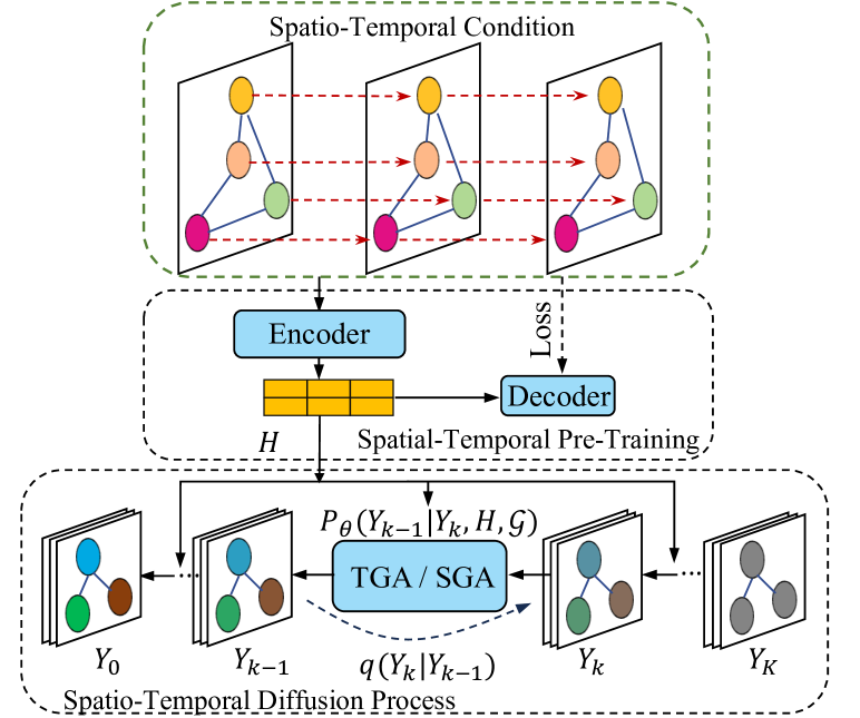
Figure 2. The USTD framework comprises a pre-trained spatio-temporal encoder and attention-based denoising networks TGA and SGA for the diffusion process. $H$ is the conditional representation learned by the encoder.

3. Unified Spatio-Temporal Diffusion Models

Fig. 2 shows the overall pipeline of USTD, which consists of two major components: the pre-trained encoder and the task-specific denoising networks for diffusion processes. The encoder aims to learn high-quality representations of conditional information while the diffusion processes generate predictions using denoising networks under the prop of the representations.

3.1. Pre-Trained Saptio-Temporal Encoder

Conditional information contains abundant spatio-temporal dependencies that play a vital role and can be shared in spatio-temporal tasks. Moreover, it is deterministic and should be pre-extracted effectively for the benefit of subsequent probabilistic models. Based on this insight, we propose to pre-train an encoder based on the unsupervised autoencoding strategy (Hinton and Zemel, 1993). As shown in Fig. 3, it employs the encoder to acquire conditional representations of the data in a latent space, with an auxiliary decoder to reconstruct the data from the space. The learned latent space has demonstrated effectiveness in capturing data correlations, thereby facilitating downstream tasks (Liu et al., 2023b; Kipf and Welling, 2016). Here, we first introduce the network architecture and then discuss the graph sampling and masking strategies to enhance the model’s learning capability.

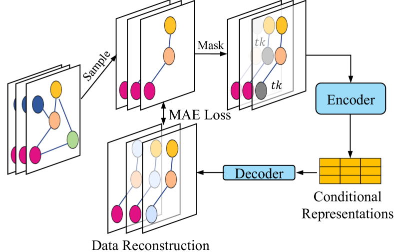
Figure 3. Pipeline of the spatio-temporal encoder, where $tk$ denotes the mask token.

Encoder

The encoder consists of a stack of STGNN blocks, with each capturing spatial and temporal correlations. In each block, we first employ a temporal convolution network (TCN) for temporal dependencies. Specifically, a gated 1D convolution (Wu et al., 2019) takes conditional representations $H_{i}\in\mathbb{R}^{T\times d_{h}}$ from the last layer as input:

(7) $$H_{i}=H_{i}\star\mathcal{K}_{1}\odot\sigma(H_{i}\star\mathcal{K}_{2}),$$

where $\star\mathcal{K}_{1}$ and $\star\mathcal{K}_{2}$ are convolutions with a kernel size of $c\times d_{h}\times d_{out}$ and $\odot$ is the Hadamard product. Then, graph convolution network (GCN) (Kipf and Welling, 2017) is utilized to capture spatial relations, which can be formulated as:

(8) $$H=\sum_{l=0}^{L}A^{l}HW_{l},$$

where $W_{l}\in\mathbb{R}^{d_{h}\times d_{out}}$ is a learnable matrix and $l$ is the depth of graph propagation. Meanwhile, skip and residual connections are added to transfer information at different layers.

To obtain conditional representations in the latent space, the encoder takes in conditional information $X\in\mathbb{R}^{N\times T\times d_{x}}$ and yields the representations $H\in\mathbb{R}^{N\times\tau\times d_{h}}$. Note that we do not use zero padding for TCNs so the temporal dimension is squashed with $\tau<<T$. In this way, the condition is mapped into a low-dimensional latent space containing representative information. Moreover, taking the low-dimensional representations as the input, the denoising network requires less computation, decreasing diffusion’s well-known prolonged sampling time (Tashiro et al., 2021; Liu et al., 2023a).

Decoder

The decoder is a lightweight network to reconstruct the original conditional data from the learned representations. It contains a small stack of spatio-temporal blocks introduced above that takes in the representations $H\in\mathbb{R}^{N\times\tau\times d_{h}}$ and outputs $H\in\mathbb{R}^{N\times 1\times d_{h}}$. Then, a multi-layer perceptron layer is used to obtain the reconstruction $\hat{X}\in\mathbb{R}^{N\times T\times d_{x}}$. The encoder and decoder are optimized by minimizing the mean absolute error loss between the ground truth $X$ and the reconstruction $\hat{X}$.

Graph Sampling

As the number of observed nodes might be dynamic in the kriging task (Wu et al., 2021c), it is crucial for the encoder to generalize to various graph structures. Here, we employ a simple graph sampling mechanism. For each iteration, we sample a subset of nodes $\bar{\mathcal{V}}\in\mathcal{V}$. Then, the new graph $\bar{\mathcal{G}}$ and its adjacency matrix $\bar{A}$ are constructed. The training objective is altered to reconstruct signals of nodes in the sampled graph. In this way, the model is unable to capture spatio-temporal relations by memorizing the graph structure, resulting in an increase in generalizability.

Masking

The dimension $d_{h}$ of the latent space is much larger than the node channel $d_{x}$; thus, the model risks learning a trivial solution that identically maps node data into the space (Grill et al., 2020). To alleviate the problem, we utilize a masking strategy that randomly corrupts the conditional information during training (He et al., 2022). We sample a binary mask $MSK\in\{0,1\}^{N\times T}$, where $1$ indicates data to be corrupted. Then, the data is masked with a learnable token $tk\in\mathbb{R}^{d_{x}}$, which can be defined as:

(9) $$\bar{x}_{i}^{t}=\begin{cases}x_{i}^{t}&MSK_{i}^{t}=0\\ tk&MSK_{i}^{t}=1\end{cases},$$

where $\bar{x}_{i}^{t}$ is the masked data. Accordingly, the loss is changed to measure the masked signals of nodes in the sampled graph, given the partially observed node data $\bar{X}$ and the matrix $\bar{A}$. Following MAE (He et al., 2022), we use a high mask ratio of 75%, forcing the model to extract dependencies from scarce signals and learn meaningful node representations.

3.2. Spatio-Temporal Diffusion Process

Spatio-temporal graph learning tasks can be viewed as modeling conditional distributions given learned representations. To learn such distributions, we leverage denoising diffusion modeling (Ho et al., 2020). We first introduce the formulation, training, and inference procedures for conditional DDPM in our tasks, followed by the descriptions of the task-specific denoising networks TGA and SGA.

Conditional Diffusion Formulation

Given the prediction target $Y\in\mathbb{R}^{N\times T^{\prime}\times d_{y}}$ for forecasting or $Y\in\mathbb{R}^{M\times T\times d_{y}}$ for kriging, the diffusion process first transforms it into a sequence of variables $(Y_{0},..,Y_{k},..,Y_{K})$ with $Y_{0}=Y$. Specifically, Gaussian noises are gradually added to $Y_{k}$ such that $Y_{K}$ is a standard Gaussian, which is the same as DDPM’s forward process in Eq. 3. Then, the reverse process employs a denoising network to reconstruct the target distribution based on conditional representations and the graph structure. The process samples a target from standard Gaussian at the first step and then progressively predicts a less noisy one, which can be expressed as:

(10) $$p_{\theta}\left(Y_{0:K}|H,\mathcal{G}\right)=p\left(Y_{K}\right)\prod_{k=1}^{K}p_{\theta}\left(Y_{k-1}\mid Y_{k},H,\mathcal{G}\right),$$

where $\theta$ is the parameters of the denoising network.

Training

The model can be optimized by variational approximation with the simplified loss in Eq. 6 as follows:

(11) $$\mathcal{L}(\theta)=-\mathbb{E}_{Y_{0},\epsilon,k}\left\|\epsilon-\epsilon_{\theta}\left(\sqrt{\alpha_{k}}Y_{0}+\sqrt{1-\alpha_{k}}\epsilon,H,\mathcal{G},k\right)\right\|_{2}^{2},$$

where $\epsilon\sim\mathcal{N}\left(0,\boldsymbol{I}\right)$ is a random noise and $\epsilon_{\theta}(\cdot)$ is the denoising network described in the following section. The complete training procedure is summarized in Algorithm 1.

Algorithm 1 Training for denoising networks

0:  Distribution of training data $q(Y)$, graph $\mathcal{G}$, pre-trained encoder $\operatorname{Enc}_{\phi}(\cdot)$

0:  Trained denoising function $\epsilon_{\theta}(\cdot)$

1:  repeat

2:     $Y_{0}\sim q(Y)$, $k\sim Uniform(1,..,K)$, $\epsilon\sim\mathcal{N}(0,\boldsymbol{I})$

3:     Get conditional information $X$ from the dataset given $Y_{0}$, learn representations $H$ from the encoder $\operatorname{Enc}_{\phi}(X,\mathcal{G})$

4:     Take gradient descent step  $\nabla_{\theta}\left\|\epsilon-\epsilon_{\theta}\left(\sqrt{\alpha_{k}}Y_{0}+\sqrt{1-\alpha_{k}}\epsilon,H,\mathcal{G},k\right)\right\|_{2}^{2}$

5:  until Converged

Inference

During inference, we first extract the conditional representations $H$ by the pre-trained encoder. Then, conditioned on $H$, a standard Gaussian sample is denoised progressively along the reversed chain to predict the target. The process of each denoising step is formulated as follows:

(12) $$Y_{k-1}=\frac{1}{\sqrt{\hat{\alpha}_{k}}}\left(Y_{k}-\frac{\beta_{k}}{\sqrt{1-\alpha_{k}}}\epsilon_{\theta}\left(Y_{k},H,\mathcal{G},k\right)\right)+\sqrt{\beta_{k}}Z,$$

where $Z$ is a standard Gaussian noise. Algorithm 2 describes the full procedure of the inference process.

Algorithm 2 Sampling target $Y$

0:  Conditional information $X$, graph $\mathcal{G}$, denoising network $\epsilon_{\theta}(\cdot)$, encoder $\operatorname{Enc}_{\phi}(\cdot)$

0:  Inference target $Y$

1:  Get conditional representations $H$ from the pre-trained encoder $\operatorname{Enc}\phi(X,\mathcal{G})$

2:  $Y_{K}\sim\mathcal{N}(0,\boldsymbol{I})$, $Z\sim\mathcal{N}(0,\boldsymbol{I})$ if $k>1$ else $Z=0$

3:  for $k=K$ to $1$ do do

4:     $Y_{k-1}=\frac{1}{\sqrt{\hat{\alpha}_{k}}}\left(Y_{k}-\frac{\beta_{k}}{\sqrt{1-\alpha_{k}}}\epsilon_{\theta}\left(Y_{k},H,\mathcal{G},k\right)\right)+\sqrt{\beta_{k}}Z,$

5:  end for

6:  return  $Y_{0}$

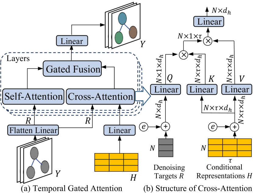
Figure 4. (a) Architecture of the proposed Temporal Gated Attention Network. (b) Pipeline of the cross-attention, where $e$ denotes time and diffusion embeddings.

3.2.1. Temporal Gated Attention Network

The denoising network is crucial in predicting the target by capturing its dependencies with conditional representations. Given that forecasting predicts future signals based on historical data, with a focus on temporal relations, we assume the denoising network is spatially independent. Based on this assumption, we propose a temporal gated attention network (TGA), whose network architecture is shown in Fig. 4(a). Given the predicted target $Y\in\mathbb{R}^{N\times T^{\prime}\times d_{y}}$ at the previous diffusion step, we first obtain its flattened feature embeddings $R\in\mathbb{R}^{N\times d_{h}}$ by a linear layer. Then, as shown in Fig. 4(b), a cross-attention block (Vaswani et al., 2017) is leveraged to measure the dependencies between $R_{i}\in\mathbb{R}^{d_{h}}$ of the node $i$ and its historical representations $H_{i}\in\mathbb{R}^{\tau\times d_{h}}$:

(13) $$\begin{split}&Q_{i}=W_{cq}R_{i},\quad K_{i}=W_{ck}H_{i},\quad V_{i}=W_{cv}H_{i},\\ &R^{ca}_{i}=\operatorname{softmax}\left(\frac{Q_{i}K_{i}^{T}}{\sqrt{d_{h}}}\right)V_{i},\end{split}$$

where $R_{i}^{ca}\in\mathbb{R}^{d_{h}}$ is node $i$’s outputs, $W_{cq}$, $W_{ck}$, $W_{cv}$ are learnable matrices. Note that the attention is performed independently for each node. Next, to capture the correlations among the embeddings $R_{i}$ of nodes, we introduce a self-attention block implementing $R^{sa}=\operatorname{softmax}\left(\frac{QK^{T}}{\sqrt{d_{h}}}\right)V$ with:

(14) $$Q=W_{sq}R,\quad K=W_{sk}R,\quad V=W_{sv}R,$$

where $R^{sa}\in\mathbb{R}^{N\times d_{h}}$ is the self-attention outputs. Then, a gated fusion mechanism is proposed to integrate the outputs:

(15) $$\begin{split}&R=Gate\odot R^{ca}+(1-Gate)\odot R^{sa},\\ &Gate=\sigma\left(R^{ca}W_{g1}+R^{sa}W_{g2}+b_{g}\right),\end{split}$$

where $W_{g1},W_{g1},b_{g}$ are parameters and $\sigma(\cdot)$ is a sigmoid function. The gated attention can be stacked with several layers. In the end, we utilize a linear layer to get the prediction of the current diffusion step. Under the assumption, the module only captures dependencies on the most important dimension, thereby reducing its complexity. Meanwhile, the two attentions independently address two distinct types of relationships, thereby enhancing the learning of conditional distributions.

3.2.2. Spatial Gated Attention Network

For kriging, we similarly assume temporal independence and propose spatial gated attention (SGA) with two differences from TGA. First, we employ an embedding layer to absorb the temporal dimension of the conditional representations such that $H\in\mathbb{R}^{N\times d_{h}}$. Second, the cross-attention captures dependencies between representations and the target nodes on the spatial dimension and obtains the outputs $R^{ca}\in\mathbb{R}^{M\times d_{h}}$. The rest parts remain the same with TGA’s structure. Note that following the previous work (Tashiro et al., 2021), we enhance the attention of TGA and SGA by incorporating diffusion, time, or space embeddings as additional learning contexts.

4. Experiments

4.1. Datasets

We evaluate USTD on four real-world datasets from two spatio-temporal domains and Table 1 provides a summary of the datasets:

• Traffic: PEMS-03 (Song et al., 2020) provides measurements of traffic flow, offering information into the dynamic traffic conditions within the San Francisco Bay Area. PEMS-BAY (Li et al., 2018) contains traffic speed information from the same area.

• Air Quality: AIR-BJ and AIR-GZ compile one-year data on air quality indexes (AQI) from monitoring stations in the cities of Beijing and Guangzhou. In our experiments, we focus on the most critical index PM2.5.

Table 1. Statistics of the datasets. # denotes the number of.

Dataset	#Node	#Time Step	Granularity	Attribute
PEMS-03	358	26,208	5 min	Flow
PEMS-BAY	325	52,116	5 min	Speed
AIR-BJ	36	8,760	1 hour	PM2.5
AIR-GZ	42	8,760	1 hour	PM2.5

Table 2. Performance comparison of USTD and baselines on the forecasting task. The results are averaged over all predicted time steps, where smaller metrics mean better performance. The bold and underline are the best and second-best results.

Method	PEMS-03			PEMS-BAY			AIR-BJ			AIR-GZ
	MAE	RMSE	CRPS	MAE	RMSE	CRPS	MAE	RMSE	CRPS	MAE	RMSE	CRPS
STGCN	17.49	30.12	_	1.88	4.30	_	31.09	49.16	_	12.80	18.26	_
STSGCN	17.48	29.21	_	1.79	3.91	_	31.00	49.46	_	12.02	18.59	_
STGODE	16.50	27.84	_	1.77	3.33	_	30.28	48.26	_	10.89	15.73	_
STGNCDE	15.57	27.09	_	1.68	3.66	_	30.45	49.17	_	10.10	15.90	_
GMSDR	15.78	26.82	_	1.69	3.80	_	32.15	51.08	_	11.78	17.72	_
TimeGrad	21.55	36.57	0.101	2.62	5.30	0.034	33.40	54.93	0.363	15.45	21.93	0.376
MC Dropout	18.87	29.81	0.093	3.50	5.43	0.040	37.92	55.49	0.391	13.10	19.26	0.290
CSDI	23.46	39.60	0.098	2.67	4.10	0.031	38.94	57.81	0.417	14.78	22.24	0.361
PriSTI	22.30	37.58	0.092	2.51	3.99	0.026	36.81	54.34	0.388	14.04	21.03	0.352
USTD	15.32	26.06	0.087	1.63	3.55	0.022	30.09	47.65	0.348	9.70	15.08	0.257
Improvement	1.6%	2.8%	5.4%	3.0%	_	15.4%	1.2%	1.3%	4.1%	4.0%	4.1%	11.4%

Table 3. Performance comparison of USTD and baselines on the kriging task.

Method	PEMS-03			PEMS-BAY			AIR-BJ			AIR-GZ
	MAE	RMSE	CRPS	MAE	RMSE	CRPS	MAE	RMSE	CRPS	MAE	RMSE	CRPS
ADAIN	16.93	38.47	_	3.35	6.32	_	15.04	29.59	_	10.28	15.37	_
KCN	16.01	37.35	_	2.63	5.17	_	14.88	28.98	_	9.81	15.06	_
IGNNK	15.50	36.17	_	2.30	4.58	_	13.86	27.48	_	8.95	13.76	_
INCREASE	15.34	35.95	_	2.19	4.51	_	14.10	28.48	_	8.82	13.58	_
CSDI	15.09	35.73	0.082	2.35	4.62	0.032	14.14	28.97	0.135	9.62	14.65	0.246
PriSTI	14.95	35.42	0.076	2.06	4.29	0.026	13.78	27.86	0.133	8.98	14.13	0.231
USTD	14.73	34.94	0.071	1.96	4.22	0.025	13.30	27.09	0.130	8.61	13.10	0.213
Improvement	1.4%	1.4%	6.6%	4.9%	1.6%	4.0%	3.5%	1.4%	3.7%	2.4%	3.5%	7.8%

4.2. Baselines

We consider the following baselines for the two tasks.

• Forecasting: STGCN (Yu et al., 2018), STSGCN (Song et al., 2020), GMSDR (Liu et al., 2022) are popular STGNN variants that propose various mechanism to enhance the performance. STGNCDE (Choi et al., 2022), STGODE (Fang et al., 2021) are spatio-temporal networks empowered by neural differential equations. MC Dropout (Wu et al., 2021a) utilizes Monte Carlo dropout to estimate uncertainties. CSDI (Tashiro et al., 2021), PriSTI (Liu et al., 2023a) and TimeGrad (Rasul et al., 2021) are recently published diffusion methods.

• Kriging: ADAIN (Cheng et al., 2018) is a sequential method using RNNs for temporal dependencies while KCN (Appleby et al., 2020) is a spatial model based on GNNs. IGNNK (Wu et al., 2021b) leverage GNNs to spatial and temporal correlations simultaneously when predicting signals. INCREASE (Zheng et al., 2023) explicitly capture types of the spatial relations. Diffusion models CSDI and PriSTI are also applicable to the kriging task.

Among the above baselines, MC Dropout, CSDI, PriSTI and TimeGrad are probabilistic models with uncertainty estimates while the rest are deterministic neural networks.

4.3. Experiment Setups and Evaluation Metrics

For the forecasting task, we follow the settings (Song et al., 2020; Yu et al., 2018), where the previous $T=12$ time steps are used to predict the subsequent $T^{\prime}=12$ steps. We partition all datasets into three temporal segments: training, validation, and testing with the split ratios of $6:2:2$ for PEMS-03 and $7:2:1$ for the remaining datasets. Regarding the kriging problem, we spatially partition the data into observed locations and target nodes at a ratio of $N:M=2:1$. The time window $T$ is also set to $12$. For hyperparameters, the encoder consists of 6 layers mapping data into a 64-size latent space, and the decoder has 3 layers. The graph sampling rate is fixed to 80%. TGA and SGA, trained individually, each has 2 layers with a 96-size channel, incorporating temporal (Zhou et al., 2021b) and spatial (Dwivedi and Bresson, 2020) embeddings. Following (Liu et al., 2023b), we finetune the encoder when training the denoising modules. Diffusion settings are consistent with (Tashiro et al., 2021). We conduct each experiment 3 times, reporting average results.

We utilize Mean Absolute Error (MAE) and Root Mean Squared Error (RMSE) as evaluation metrics. Moreover, we report the Continuous Ranked Probability Score (CRPS) by 8 sampling for probabilistic methods (Matheson and Winkler, 1976), which uses target signals to measure the compatibility of an estimated probability distribution of the models.We will release the source code on GitHub for public use after the paper is accepted.

4.4. Performance Comparison

Table 2 and 3 compare the performances of USTD and the baselines on the two tasks. From the tables, we observe that USTD consistently outperforms all probabilistic methods with a notable margin. Compared to the second-best probabilistic methods, our model decreases CRPS by 4.1% – 15.4% on forecasting and 3.7% – 7.8% on kriging, which indicates our model has a better ability to capture uncertainties. When it comes to deterministic baselines, our model still can surpass them clearly only except for the RMSE of STGODE on PEMS-BAY. As previous approaches found probabilistic methods are hard to surpass deterministic counterparts (Wen et al., 2023), the performances of USTD are compelling here. Numerically, compared to the second-best models, our framework reduces the MAE by 1.6% – 4.0% and 1.4% – 4.9% on two tasks, respectively.

From the tables, we also have the following observations and explanations: (i) Probabilistic baselines struggle to outperform deterministic networks, especially for forecasting that has more well-explored methods, which is consistent with the previous findings. As these baselines optimize the encoder together with denoising networks, the increased training difficulties hamper their performance. (ii) They gain improved performance on the spatial prediction task–kriging, particularly for PriSTI. This is likely because the graph information it utilized, defining correlations between conditional and target nodes, serves as an extra prior that facilitates spatial learning. (iii) Our USTD, as a probabilistic method, outperforms the deterministic baselines. This suggests the pre-trained encoder learns representative conditional information, alleviating the learning difficulties for the subsequent denoising module.

4.5. Inference Time

Diffusion-based models bear a notorious long inference time during testing, partially due to the recurrent sampling manner on the chain. As our denoising modules take in low-dimensional conditional representations, they demand less computation and should have a faster inference time. To justify this property, we compare the time of USTD with CSDI and PriSTI, where the time indicates the cost of one target prediction, and conduct the study on two datasets with the largest number of nodes. From Table 4, we find USTD enjoys a faster computation speed, which reduces the time by at most 47.3% compared to the second best. As our model follows the same sampling procedure with the baselines but relies on the compressed conditional information, this finding suggests that a more efficient denoising network can significantly reduce the inference time.

Table 4. Inference time (seconds) of diffusion models.

Method	PEMS-03		PEMS-BAY
	Forecasting	Kriging	Forecasting	Kriging
CSDI	0.877	0.898	0.931	0.852
PriSTI	1.133	1.045	1.047	1.022
USTD	0.501	0.496	0.490	0.487
Improvement	43.5%	44.8%	47.3%	42.8%

4.6. Case Study

To gain insights into the uncertainty estimates and prediction accuracy, we conduct case studies to visualize the results of USTD and the baselines on the forecasting task. Fig. 5(a) and 5(b) present the prediction of $T^{\prime}=12$ future time steps based on $T=12$ historical steps, from which we find USTD numerically outperforms the diffusion model CSDI, as our predictions are closer to the ground truth. In addition, regarding uncertainty estimates, our model demonstrates higher reliability because the shadow straps encompass the true signals with a narrow sampling range. This means that USTD is able to extract high-quality spatio-temporal dependencies from historical data, probably benefiting from the pre-trained encoder. In 5(c) we illustrate the successive prediction values of 1-step ahead forecasting and compare our model with deterministic baselines. As the red block indicates, USTD enjoys superiority over the other models, even when compared to the recent model GMSDR. In addition, in cases where USTD performs similarly to the baselines, as shown in the blue block, its probabilistic nature provides additional information regarding the uncertainty of predictions, which facilitates decision-making in real-world trustworthy applications.

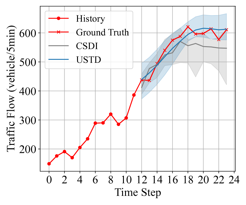
(a) Node 330 in PEMS-03

(b) Node 324 in PEMS-BAY

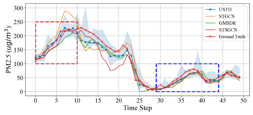
(c) Node 27 in BJ-AIR

Figure 5. Forecasting visualizations on three datasets.

4.7. Abaltion Study

Effects of Pre-Trained Encoder

To study the effects of the influence of the pre-training strategy, graph sampling, and masking on the encoder, we use the following variants: (a) w/o Encoder: we discard the encoder and only use the denoising network. (b) w/o PT: we train the encoder and the denoising network together in an end-to-end way. (c) w/o MK: We pre-train the encoder without the masking mechanism. (d) w/o GS: Graph sampling is not involved in the training. Fig. 6 shows the results on the two tasks. Removing the encoder leads to the worst performance deterioration, verifying the importance of effectively modeling conditional dependencies. Then, pre-training the encoder also plays a crucial role, which pre-extracts dependencies and reduces learning difficulties for the denoising module. Moreover, masking benefits both forecasting and kriging tasks and prevents the model from obtaining trivial solutions. Then, graph sampling boosts the model’s performance in kriging, as the encoder is required to adapt to dynamic graph structures.

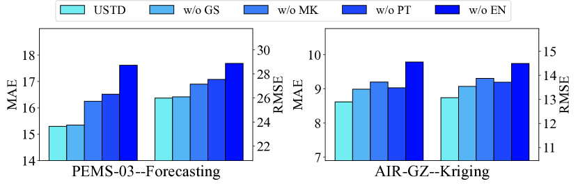
Figure 6. Effects of the pre-trained encoder.

Effects of Gated Attention Networks

We consider four variants to examine the efficacy of gated attention networks. (a) r/p TCN: We replace the cross-attention in TGA with a temporal convolutional network. (b) r/p GNN: SGA’s cross-attention is substituted with a GNN. (c) w/o SA: The self-attention block is detached. (d) r/p TF: This variant replaces the two attentions with a standard transformer layer to assess the independence assumption. The results are shown in Fig. 7, in which we find that r/p TCN and w/o SA lead to the largest performance degradation. This is because TCN’s kernel requires evenly temporal evolution that is not satisfied by concatenating representations and the targets. Moreover, self-attention plays an exclusive role in capturing correlations among the targets. Both r/p TF and r/p GNN cause a slight performance deterioration, demonstrating the effectiveness of the assumption and USTD’s ability to capture spatial relations.

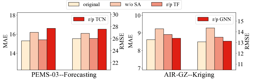
Figure 7. Effects of the gated attention networks.

4.8. Hyperparameter Study

We first study the effects of the number of encoder layers $L_{EN}$, TGA blocks $L_{TGA}$, and the channel size $h$ of the blocks on forecasting. Fig. 8(a) reports the results on PEMS-03 and we have the following observations: 1) Stacking 6 encoder layers achieves the best, while the model is overfitting clearly with $L_{EN}=9$. 2) The performance of USTD is not sensitive when $L_{TGA}>1$ and $h>64$. Hereby, the TGA module has 2 layers with a channel size of 96. Then, we evaluate the effects on the kriging task using AIR-GZ and change the number of SGA layers and the channel size. From Fig. 8(b), we find the model gets the best results when $L_{EN}=6$, $L_{TGA}=2$ and $h=96$, aligning with the settings of forecasting. The sensitivity of the encoder and denoising networks can be explained by its optimization method. As the denoising networks are trained through variational approximation, they have more opportunities to search in the training space to skip local minima.

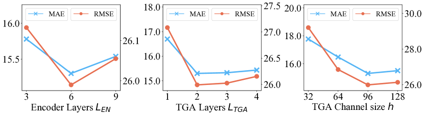
(a) Hyperparameters of forecasting on PEMS-03

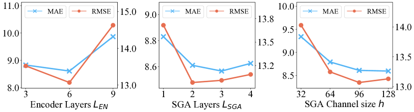
(b) Hyperparameters of kriging on AIR-GZ

Figure 8. Effects of USTD’s hyperparameters.

5. Related Work

5.1. Spatio-Temporal Graph Neural Networks

Spatio-temporal graph neural networks (STGNNs) are a popular paradigm for spatio-temporal data modeling nowadays. They serve as feature extractors to capture complex spatial and temporal dependencies in conditional information. Mainly following two categories, they first resort to graph neural networks to model spatial correlations, then combine with either temporal convolutional networks (Wu et al., 2020, 2019) or recurrent neural networks (Xu et al., 2019; Shu et al., 2020) for temporal relationship capturing. The learned conditional patterns can be used for various downstream learning tasks. For instance, (Li et al., 2018) proposed an encoder-decoder architecture for traffic flow prediction. (Deng and Hooi, 2021) introduced a structure learning approach by GNNs for multivariate time-series anomaly detection. (Shu et al., 2020) employed graph LSTMs to model multi-level dependencies for group activity recognition.

5.2. Spatio-Temporal Graph Learning

Spatio-temporal graph learning problems involve many downstream tasks. In this work, we focus on two crucial problems: forecasting and kriging. The forecasting models rely on STGNNs to capture spatio-temporal dependencies and propose various mechanisms to boost their learning effectiveness. For example, STSGCN (Song et al., 2020) captures spatial and temporal correlations simultaneously by a synchronous modeling mechanism. STGODE (Fang et al., 2021) and STGNCDE (Choi et al., 2022) rely on the neural differential equations to model long-range spatial-temporal dependencies. GMSDR (Liu et al., 2022) introduces an RNN variant that explicitly maintains multiple historical information at each time step. Similar to forecasting, kriging methods still count on STGNNs but emphasize the spatial relations between observed and target nodes, the only information available for target nodes (Appleby et al., 2020; Wu et al., 2021b). These relations are typically modeled by various graph aggregators. KCN (Appleby et al., 2020) utilizes a mask to indicate the target node in the aggregator. SATCN (Wu et al., 2021c) extracts statistical properties of the target nodes while INCREASE (Zheng et al., 2023) utilizes external features like POIs to capture spatial relations. Although these methods achieve promising performances, they still solve the problems separately with dedicated designs and fail to estimate the uncertainties.

5.3. Spatio-Temporal Diffusion Models

DDPMs are initially proposed for computer vision as a generative model, given their strong capabilities in modeling complex data distributions (Ho et al., 2020). Recently, the community has started to explore its potential for spatio-temporal learning tasks (Lin et al., 2023). TimeGrad (Rasul et al., 2021) is a pioneer diffusion work for time-series forecasting, which suffers from a huge inference time due to its autoregressive nature. DiffSTG (Wen et al., 2023) utilizes a U-net architecture with a non-autoregressive design to speed up sampling. CSDI (Tashiro et al., 2021) is proposed for data imputation based on spatio-temporal transformers and PriSTI (Liu et al., 2023a) further adds a GNN layer to capture graph dependencies. As an early-stage exploration, these methods fail to pre-extract conditional patterns effectively to benefit probabilistic denoising networks.

6. Conclusion

We present USTD as the first step towards unifying spatio-temporal graph learning. Our model leverages a pre-trained encoder to effectively extract conditional spatio-temporal dependencies for the subsequent denoising networks. Then, attention-based denoising modules TGA and SGA are introduced to generate predictions for forecasting and kriging, respectively. Compared to both deterministic and probabilistic methods, our USTD achieves state-of-the-art performances while providing valuable uncertainty estimates. Meanwhile, its holistic design also holds practical potential as a universal solution for many Web applications. One promising direction for future research would be to explore the feasibility of training a single model that can be universally applied to various spatio-temporal learning tasks.

References

- (1)
- Alcaraz and Strodthoff (2023) Juan Lopez Alcaraz and Nils Strodthoff. 2023. Diffusion-based Time Series Imputation and Forecasting with Structured State Space Models. Transactions on Machine Learning Research (2023).
- Appleby et al. (2020) Gabriel Appleby, Linfeng Liu, and Li-Ping Liu. 2020. Kriging convolutional networks. In Proceedings of the AAAI Conference on Artificial Intelligence, Vol. 34. 3187–3194.
- Bermudez-Edo and Barnaghi (2018) Maria Bermudez-Edo and Payam Barnaghi. 2018. Spatio-temporal analysis for smart city data. In Companion Proceedings of the The Web Conference 2018. 1841–1845.
- Cheng et al. (2018) Weiyu Cheng, Yanyan Shen, Yanmin Zhu, and Linpeng Huang. 2018. A neural attention model for urban air quality inference: Learning the weights of monitoring stations. In AAAI. 2151–2158.
- Choi et al. (2022) Jeongwhan Choi, Hwangyong Choi, Jeehyun Hwang, and Noseong Park. 2022. Graph neural controlled differential equations for traffic forecasting. In Proceedings of the AAAI Conference on Artificial Intelligence, Vol. 36. 6367–6374.
- Deng and Hooi (2021) Ailin Deng and Bryan Hooi. 2021. Graph neural network-based anomaly detection in multivariate time series. In Proceedings of the AAAI conference on artificial intelligence, Vol. 35. 4027–4035.
- Dwivedi and Bresson (2020) Vijay Prakash Dwivedi and Xavier Bresson. 2020. A generalization of transformer networks to graphs. arXiv preprint arXiv:2012.09699 (2020).
- Fang et al. (2021) Zheng Fang, Qingqing Long, Guojie Song, and Kunqing Xie. 2021. Spatial-temporal graph ode networks for traffic flow forecasting. In Proceedings of the 27th ACM SIGKDD conference on knowledge discovery & data mining. 364–373.
- Graells-Garrido et al. (2020) Eduardo Graells-Garrido, Irene Meta, Feliu Serra-Buriel, Patricio Reyes, and Fernando M Cucchietti. 2020. Measuring spatial subdivisions in urban mobility with mobile phone data. In Companion Proceedings of the Web Conference 2020. 485–494.
- Grill et al. (2020) Jean-Bastien Grill, Florian Strub, Florent Altché, Corentin Tallec, Pierre Richemond, Elena Buchatskaya, Carl Doersch, Bernardo Avila Pires, Zhaohan Guo, Mohammad Gheshlaghi Azar, et al. 2020. Bootstrap your own latent-a new approach to self-supervised learning. Advances in neural information processing systems (2020), 21271–21284.
- He et al. (2022) Kaiming He, Xinlei Chen, Saining Xie, Yanghao Li, Piotr Dollár, and Ross Girshick. 2022. Masked autoencoders are scalable vision learners. In Proceedings of the IEEE/CVF Conference on Computer Vision and Pattern Recognition. 16000–16009.
- Hinton and Zemel (1993) Geoffrey E Hinton and Richard Zemel. 1993. Autoencoders, minimum description length and Helmholtz free energy. Advances in neural information processing systems 6 (1993).
- Ho et al. (2020) Jonathan Ho, Ajay Jain, and Pieter Abbeel. 2020. Denoising diffusion probabilistic models. Advances in Neural Information Processing Systems 33 (2020), 6840–6851.
- Hu et al. (2023) Junfeng Hu, Yuxuan Liang, Zhencheng Fan, Hongyang Chen, Yu Zheng, and Roger Zimmermann. 2023. Graph Neural Processes for Spatio-Temporal Extrapolation. In Proceedings of the 29th ACM SIGKDD Conference on Knowledge Discovery and Data Mining.
- Huang et al. (2022) H. Huang, L. Sun, B. Du, Y. Fu, and W. Lv. 2022. GraphGDP: Generative Diffusion Processes for Permutation Invariant Graph Generation. In 2022 IEEE International Conference on Data Mining (ICDM). 201–210.
- Jin et al. (2023) Guangyin Jin, Yuxuan Liang, Yuchen Fang, Jincai Huang, Junbo Zhang, and Yu Zheng. 2023. Spatio-temporal graph neural networks for predictive learning in urban computing: A survey. arXiv preprint arXiv:2303.14483 (2023).
- Kipf and Welling (2016) Thomas N Kipf and Max Welling. 2016. Variational graph auto-encoders. arXiv preprint arXiv:1611.07308 (2016).
- Kipf and Welling (2017) Thomas N. Kipf and Max Welling. 2017. Semi-Supervised Classification with Graph Convolutional Networks. In 5th International Conference on Learning Representations, ICLR.
- Li et al. (2018) Yaguang Li, Rose Yu, Cyrus Shahabi, and Yan Liu. 2018. Diffusion Convolutional Recurrent Neural Network: Data-Driven Traffic Forecasting. In International Conference on Learning Representations (ICLR ’18).
- Lin et al. (2023) Lequan Lin, Zhengkun Li, Ruikun Li, Xuliang Li, and Junbin Gao. 2023. Diffusion Models for Time Series Applications: A Survey. arXiv preprint arXiv:2305.00624 (2023).
- Liu et al. (2022) Dachuan Liu, Jin Wang, Shuo Shang, and Peng Han. 2022. Msdr: Multi-step dependency relation networks for spatial temporal forecasting. In Proceedings of the 28th ACM SIGKDD Conference on Knowledge Discovery and Data Mining. 1042–1050.
- Liu et al. (2023a) Mingzhe Liu, Han Huang, Hao Feng, Leilei Sun, Bowen Du, and Yanjie Fu. 2023a. PriSTI: A Conditional Diffusion Framework for Spatiotemporal Imputation. arXiv preprint arXiv:2302.09746 (2023).
- Liu et al. (2023b) Mingzhe Liu, Tongyu Zhu, Junchen Ye, Qingxin Meng, Leilei Sun, and Bowen Du. 2023b. Spatio-Temporal AutoEncoder for Traffic Flow Prediction. IEEE Transactions on Intelligent Transportation Systems (2023).
- Luo et al. (2021) Yingtao Luo, Qiang Liu, and Zhaocheng Liu. 2021. Stan: Spatio-temporal attention network for next location recommendation. In Proceedings of the web conference 2021. 2177–2185.
- Matheson and Winkler (1976) James E Matheson and Robert L Winkler. 1976. Scoring rules for continuous probability distributions. Management science (1976), 1087–1096.
- Rasul et al. (2021) Kashif Rasul, Calvin Seward, Ingmar Schuster, and Roland Vollgraf. 2021. Autoregressive denoising diffusion models for multivariate probabilistic time series forecasting. In International Conference on Machine Learning. 8857–8868.
- Schweizer et al. (2022) Vanessa Jine Schweizer, Jude Herijadi Kurniawan, and Aidan Power. 2022. Semi-automated Literature Review for Scientific Assessment of Socioeconomic Climate Change Scenarios. In Companion Proceedings of the Web Conference 2022. 789–799.
- Shu et al. (2020) Xiangbo Shu, Liyan Zhang, Yunlian Sun, and Jinhui Tang. 2020. Host–parasite: Graph LSTM-in-LSTM for group activity recognition. IEEE transactions on neural networks and learning systems 32, 2 (2020), 663–674.
- Smarzaro et al. (2017) Rodrigo Smarzaro, Tiago França de Melo Lima, and Clodoveu A Davis Jr. 2017. Could Data from Location-Based Social Networks Be Used to Support Urban Planning?. In Proceedings of the 26th International Conference on World Wide Web Companion. 1463–1468.
- Song et al. (2020) Chao Song, Youfang Lin, Shengnan Guo, and Huaiyu Wan. 2020. Spatial-temporal synchronous graph convolutional networks: A new framework for spatial-temporal network data forecasting. In Proceedings of the AAAI conference on artificial intelligence. 914–921.
- Tashiro et al. (2021) Yusuke Tashiro, Jiaming Song, Yang Song, and Stefano Ermon. 2021. CSDI: Conditional score-based diffusion models for probabilistic time series imputation. Advances in Neural Information Processing Systems 34 (2021), 24804–24816.
- Tempelmeier et al. (2019) Nicolas Tempelmeier, Yannick Rietz, Iryna Lishchuk, Tina Kruegel, Olaf Mumm, Vanessa Miriam Carlow, Stefan Dietze, and Elena Demidova. 2019. Data4urbanmobility: Towards holistic data analytics for mobility applications in urban regions. In Companion Proceedings of The 2019 World Wide Web Conference. 137–145.
- Trirat and Lee (2021) Patara Trirat and Jae-Gil Lee. 2021. Df-tar: a deep fusion network for citywide traffic accident risk prediction with dangerous driving behavior. In Proceedings of the Web Conference 2021. 1146–1156.
- Vaswani et al. (2017) Ashish Vaswani, Noam Shazeer, Niki Parmar, Jakob Uszkoreit, Llion Jones, Aidan N Gomez, Łukasz Kaiser, and Illia Polosukhin. 2017. Attention is all you need. Advances in neural information processing systems (2017).
- Wang et al. (2020) Xiaoyang Wang, Yao Ma, Yiqi Wang, Wei Jin, Xin Wang, Jiliang Tang, Caiyan Jia, and Jian Yu. 2020. Traffic flow prediction via spatial temporal graph neural network. In Proceedings of the web conference 2020. 1082–1092.
- Wen et al. (2023) Haomin Wen, Youfang Lin, Yutong Xia, Huaiyu Wan, Roger Zimmermann, and Yuxuan Liang. 2023. Diffstg: Probabilistic spatio-temporal graph forecasting with denoising diffusion models. arXiv preprint arXiv:2301.13629 (2023).
- Wu et al. (2021a) Dongxia Wu, Liyao Gao, Matteo Chinazzi, Xinyue Xiong, Alessandro Vespignani, Yi-An Ma, and Rose Yu. 2021a. Quantifying uncertainty in deep spatiotemporal forecasting. In Proceedings of the 27th ACM SIGKDD Conference on Knowledge Discovery & Data Mining. 1841–1851.
- Wu et al. (2021b) Yuankai Wu, Dingyi Zhuang, Aurelie Labbe, and Lijun Sun. 2021b. Inductive graph neural networks for spatiotemporal kriging. In Proceedings of the AAAI Conference on Artificial Intelligence. 4478–4485.
- Wu et al. (2021c) Yuankai Wu, Dingyi Zhuang, Mengying Lei, Aurelie Labbe, and Lijun Sun. 2021c. Spatial Aggregation and Temporal Convolution Networks for Real-time Kriging. arXiv preprint arXiv:2109.12144 (2021).
- Wu et al. (2020) Zonghan Wu, Shirui Pan, Guodong Long, Jing Jiang, Xiaojun Chang, and Chengqi Zhang. 2020. Connecting the dots: Multivariate time series forecasting with graph neural networks. In Proceedings of the 26th ACM SIGKDD international conference on knowledge discovery & data mining. 753–763.
- Wu et al. (2019) Zonghan Wu, Shirui Pan, Guodong Long, Jing Jiang, and Chengqi Zhang. 2019. Graph wavenet for deep spatial-temporal graph modeling. In Proceedings of the 28th International Joint Conference on Artificial Intelligence. 1907–1913.
- Xu et al. (2019) Dongkuan Xu, Wei Cheng, Dongsheng Luo, Xiao Liu, and Xiang Zhang. 2019. Spatio-Temporal Attentive RNN for Node Classification in Temporal Attributed Graphs.. In IJCAI. 3947–3953.
- Yu et al. (2018) Bing Yu, Haoteng Yin, and Zhanxing Zhu. 2018. Spatio-Temporal Graph Convolutional Networks: A Deep Learning Framework for Traffic Forecasting. In Proceedings of the Twenty-Seventh International Joint Conference on Artificial Intelligence, IJCAI. 3634–3640.
- Zhang et al. (2023) Qianru Zhang, Chao Huang, Lianghao Xia, Zheng Wang, Zhonghang Li, and Siuming Yiu. 2023. Automated Spatio-Temporal Graph Contrastive Learning. In Proceedings of the ACM Web Conference 2023. 295–305.
- Zheng et al. (2020) Chuanpan Zheng, Xiaoliang Fan, Cheng Wang, and Jianzhong Qi. 2020. Gman: A graph multi-attention network for traffic prediction. In Proceedings of the AAAI conference on artificial intelligence. 1234–1241.
- Zheng et al. (2023) Chuanpan Zheng, Xiaoliang Fan, Cheng Wang, Jianzhong Qi, Chaochao Chen, and Longbiao Chen. 2023. INCREASE: Inductive Graph Representation Learning for Spatio-Temporal Kriging. In Proceedings of the ACM Web Conference 2023, WWW. 673–683.
- Zhou et al. (2021b) Haoyi Zhou, Shanghang Zhang, Jieqi Peng, Shuai Zhang, Jianxin Li, Hui Xiong, and Wancai Zhang. 2021b. Informer: Beyond efficient transformer for long sequence time-series forecasting. In Proceedings of the AAAI conference on artificial intelligence. 11106–11115.
- Zhou et al. (2021a) Zhengyang Zhou, Yang Wang, Xike Xie, Lei Qiao, and Yuantao Li. 2021a. STUaNet: Understanding uncertainty in spatiotemporal collective human mobility. In Proceedings of the Web Conference 2021. 1868–1879.