Abstract

Normalizing Flows are generative models that directly maximize the likelihood. Previously, the design of normalizing flows was largely constrained by the need for analytical invertibility. We overcome this constraint by a training procedure that uses an efficient estimator for the gradient of the change of variables formula. This enables any dimension-preserving neural network to serve as a generative model through maximum likelihood training. Our approach allows placing the emphasis on tailoring inductive biases precisely to the task at hand. Specifically, we achieve excellent results in molecule generation benchmarks utilizing $E(n)$-equivariant networks. Moreover, our method is competitive in an inverse problem benchmark, while employing off-the-shelf ResNet architectures.

1 INTRODUCTION

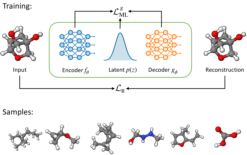
Figure 1: Free-form flows (FFF) train a pair of encoder and decoder neural networks with a fast maximum likelihood estimator $\mathcal{L}_{\operatorname{ML}}^{g}$ and reconstruction loss $\mathcal{L}_{\operatorname{R}}$. This enables training any dimension-preserving architecture as a one-step generative model. For example, an equivariant graph neural network can be trained on the QM9 dataset to generate molecules by predicting atom positions and properties in a single decoder evaluation. (Bottom) Stable molecules sampled from our $E(3)$-FFF trained on the QM9 dataset for several molecule sizes.

Generative models have actively demonstrated their utility across diverse applications, successfully scaling to high-dimensional data distributions in scenarios ranging from image synthesis to molecule generation (Rombach et al.,, 2022; Hoogeboom et al.,, 2022). Normalizing flows (Dinh et al.,, 2014; Rezende and Mohamed,, 2015) have helped propel this advancement, particularly in scientific domains, enabling practitioners to optimize data likelihood directly and thereby facilitating a statistically rigorous approach to learning complex data distributions. A major factor that has held normalizing flows back as other generative models (notably diffusion models) increase in power and popularity has been that their expressivity is greatly limited by architectural constraints, namely those necessary to ensure bijectivity and compute Jacobian determinants.

In this work, we contribute an approach that frees normalizing flows from their conventional architectural confines, thereby introducing a flexible new class of maximum likelihood models. For model builders, this shifts the focus away from meeting invertibility requirements towards incorporating the best inductive biases to solve the problem at hand. Our aim is that the methods introduced in this paper will allow practitioners to spend more time incorporating domain knowledge into their models, and allow more problems to be solved via maximum likelihood estimation.

The key methodological innovation is the adaptation of a recently proposed method for training autoencoders (Sorrenson et al.,, 2023) to dimension-preserving models. The trick is to estimate the gradient of the encoder’s Jacobian log-determinant by a cheap function of the encoder and decoder Jacobians. We show that in the full-dimensional context many of the theoretical difficulties that plagued the interpretation of the bottlenecked autoencoder model disappear, and the optimization can be interpreted as a relaxation of normalizing flow training, which is tight at the original solutions.

In molecule generation, where rotational equivariance has proven to be a crucial inductive bias, our approach outperforms traditional normalizing flows and generates valid samples more than an order of magnitude faster than previous approaches. Further, experiments in simulation-based inference (SBI) underscore the model’s versatility. We find that our training method achieves competitive performance with minimal fine-tuning requirements.

In summary our contributions are as follows:

• We remove all architectural constraints from normalizing flows by introducing maximum-likelihood training for free-form architectures. We call our model the free-form flow (FFF), see figs. 1 and 3.

• We prove that the training has the same minima as traditional normalizing flow optimization, provided that the reconstruction loss is minimal, see section 4.

• We demonstrate competitive performance with minimal fine-tuning on inverse problems and molecule generation benchmarks, outperforming ODE-based models in the latter. Compared to a diffusion model, our model produces stable molecules more than two orders of magnitude faster. See section 5.

2 RELATED WORK

Normalizing flows traditionally rely on specialized architectures that are invertible and have a manageable Jacobian determinant (see section 3.1). See Papamakarios et al., (2021); Kobyzev et al., (2020) for an overview.

One body of work builds invertible architectures by concatenating simple layers (coupling blocks) which are easy to invert and have a triangular Jacobian, which makes computing determinants easy (Dinh et al.,, 2014). Expressive power is obtained by stacking many layers and their universality has been confirmed theoretically (Huang et al.,, 2020; Teshima et al.,, 2020; Koehler et al.,, 2021; Draxler et al.,, 2022, 2023). Many choices for coupling blocks have been proposed such as MAF Papamakarios et al., (2017), RealNVP (Dinh et al.,, 2016), Glow (Kingma and Dhariwal,, 2018), Neural Spline Flows (Durkan et al.,, 2019), see Kobyzev et al., (2020) for an overview. Instead of analytical invertibility, our model relies on the reconstruction loss to enforce approximate invertibility.

Another line of work ensures invertibility by using a ResNet structure and limiting the Lipschitz constant of each residual layer (Behrmann et al.,, 2019; Chen et al.,, 2019). Somewhat similarly, neural ODEs (Chen et al.,, 2018; Grathwohl et al.,, 2018) take the continuous limit of ResNets, guaranteeing invertibility under mild conditions. Each of these models requires evaluating multiple steps during training and thus become quite expensive. In addition, the Jacobian determinant must be estimated, adding overhead. Like these methods, we must estimate the gradient of the Jacobian determinant, but can do so more efficiently. Flow Matching Lipman et al., (2022); Liu et al., (2022) improves training of these continuous normalizing flows in speed and quality, but still involves an expensive multi-step sampling process. By construction, our approach consists of a single model evaluation, and we put no constraints on the architecture apart from inductive biases indicated by the task at hand.

Two interesting methods (Gresele et al.,, 2020; Keller et al.,, 2021) compute or estimate gradients of the Jacobian determinant but are severely limited to architectures with exclusively square weight matrices and no residual blocks. We have no architectural limitations besides preserving dimension. Intermediate activations and weight matrices may have any dimension and any network topology is permitted.

3 METHOD

3.1 Normalizing Flows

Normalizing flows (Rezende and Mohamed,, 2015) are generative models that learn an invertible function $f_{\theta}(x):\mathbb{R}^{D}\to\mathbb{R}^{D}$ mapping samples $x$ from a given data distribution $q(x)$ to latent codes $z$. The aim is that $z$ follows a simple target distribution, typically the multivariate standard normal.

Samples from the resulting generative model $p_{\theta}(x)$ are obtained by mapping samples of the simple target distribution $p(z)$ through the inverse of the learned function:

$$x=f_{\theta}^{-1}(z)\sim p_{\theta}(x)\text{ for }z\sim p(z).$$ (1)

This requires a tractable inverse. Traditionally, this was achieved via invertible layers such as coupling blocks (Dinh et al.,, 2014) or by otherwise restricting the function class. We replace this constraint via a simple reconstruction loss, and learn a second function $g_{\phi}\approx f_{\theta}^{-1}$ as an approximation to the exact inverse.

A tractable determinant of the Jacobian of the learned function is required to account for the change in density. As a result, the value of the model likelihood is given by the change of variables formula for invertible functions:

$$p_{\theta}(x)=p(Z=f_{\theta}(x))|J_{\theta}(x)|.$$ (2)

Here, $J_{\theta}(x)$ denotes the Jacobian of $f_{\theta}$ at $x$, and $|\cdot|$ the absolute value of its determinant.

Normalizing Flows are trained by minimizing the Kullback-Leibler (KL) divergence between the true and learned distribution. This is equivalent to maximizing the likelihood of the training data:

$$\mathcal{D}_{\text{KL}}(q(x)\|p_{\theta}(x))=\mathbb{E}_{x\sim q(x)}[\log q(x)-\log p_{\theta}(x)]$$ (3)

$$=\mathbb{E}_{x\sim q(x)}[-\log p(f_{\theta}(x))-\log|J_{\theta}(x)|]+\operatorname{const}.$$ (4)

By eq. 2, this requires evaluating the determinant of the Jacobian $|J_{\theta}(x)|$ of $f_{\theta}$ at $x$. If we want to compute this exactly, we need to compute the full Jacobian matrix, requiring $D$ backpropagations through $f_{\theta}$. This linear scaling with dimension is prohibitive for most modern applications. The bulk of the normalizing flow literature is therefore concerned with building invertible architectures that are expressive and allow computing the determinant of the Jacobian more efficiently. We circumvent this via a trick that allows efficient estimation of the gradient $\nabla_{\theta}\log|J_{\theta}(x)|$, noting that this quantity is sufficient to perform gradient descent.

3.2 Gradient trick

The results of this section are an adaptation of results in Caterini et al., (2021) and Sorrenson et al., (2023).

Here, we derive how to efficiently estimate the gradient of the maximum-likelihood loss in eq. 4, even if the architecture does not yield an efficient way to compute the change of variables term $\log|J_{\theta}(x)|$. We avoid this computation by estimating the gradient of $\log|J_{\theta}(x)|$ via a pair of vector-Jacobian and Jacobian-vector products, which are readily available in standard automatic differentiation software libraries. In the remainder of this section, we give an overview over the derivation and point to the appendix for all details.

Gradient via trace estimator

Theorem 3.1.

Let $f_{\theta}:\mathbb{R}^{D}\to\mathbb{R}^{D}$ be a $C^{1}$ invertible function parameterized by $\theta$. Then, for all $x\in\mathbb{R}^{D}$:

$$\nabla_{\theta_{i}}\log|J_{\theta}(x)|=\operatorname{tr}\!\left((J_{\theta}(x))^{-1}\nabla_{\theta_{i}}J_{\theta}(x)\right).$$ (5)

The proof is by direct application of Jacobi’s formula. This is not a simplification per se, given that the RHS of eq. 5 now involves the computation of both the Jacobian as well as its inverse. However, we can estimate it via the Hutchinson trace estimator (where we omit dependence on $x$ for simplicity):

$$\operatorname{tr}\!\left(J_{\theta}^{-1}\nabla_{\theta_{i}}J_{\theta}\right) =\mathbb{E}_{v}[v^{T}J_{\theta}^{-1}(\nabla_{\theta_{i}}J_{\theta})v]$$ (6)

$$\approx\sum_{k=1}^{K}v_{k}^{T}J_{\theta}^{-1}(\nabla_{\theta_{i}}J_{\theta})v_{k}.$$ (7)

Now all we require is computing the dot products $v^{T}J_{\theta}^{-1}$ and $(\nabla_{\theta_{i}}J_{\theta})v$, where the random vector $v\in\mathbb{R}^{D}$ must have unit covariance.

Matrix inverse via function inverse

To compute $v^{T}J_{\theta}^{-1}$ we note that, when $f_{\theta}$ is invertible, the matrix inverse of the Jacobian of $f_{\theta}$ is the Jacobian of the inverse function $f_{\theta}^{-1}$:

$$J_{\theta}^{-1}(x)=(\nabla_{x}f_{\theta}(x))^{-1}=\nabla_{z}f_{\theta}^{-1}\big{(}z=f_{\theta}(x)\big{)}.$$ (8)

This means that the product $v^{T}J_{\theta}^{-1}$ is simply the dot product of the row vector $v^{T}$ with the Jacobian of $f_{\theta}^{-1}$. This vector-Jacobian product is readily available via backward automatic differentiation.

Use of stop-gradient

We are left with computing the dot product $(\nabla_{\theta_{i}}J_{\theta})v$. Since $v$ is independent of $\theta$, we can draw it into the gradient $(\nabla_{\theta_{i}}J_{\theta})v=\nabla_{\theta_{i}}(J_{\theta}v)$. This Jacobian-vector product can be again readily computed, this time with forward automatic differentiation.

In order to implement the final gradient with respect to the flow parameters $\theta$, we draw the derivative with respect to parameters out of the trace, making sure to prevent gradient from flowing to $J_{\theta}^{-1}$ by wrapping it in a stop-gradient operation SG:

$$\operatorname{tr}\!\left(J_{\theta}^{-1}\nabla_{\theta_{i}}J_{\theta}\right) =\nabla_{\theta_{i}}\operatorname{tr}(\mathtt{SG}(J_{\theta}^{-1})J_{\theta})$$ (9)

$$\approx\nabla_{\theta_{i}}\sum_{k=1}^{K}\mathtt{SG}(v_{k}^{T}J_{\theta}^{-1})J_{\theta}v_{k}.$$ (10)

Summary

The above argument shows that

$$\nabla_{\theta}\log|J_{\theta}(x)|\approx\nabla_{\theta}\sum_{k=1}^{K}\mathtt{SG}(v_{k}^{T}J_{\theta}^{-1})J_{\theta}v_{k}.$$ (11)

Instead of computing the full Jacobian $J_{\theta}(x)$, which involved as many backpropagation steps as dimensions, we are left with computing just one vector-Jacobian product and one Jacobian-vector product for each $k$. In practice, we find that setting $K=1$ is sufficient and we drop the summation over $k$ for the remainder of this paper.

This yields the following maximum likelihood training objective, whose gradients are an unbiased estimator for the true gradients from exact maximum likelihood as in eq. 4:

$$\mathcal{L}_{\text{ML}}^{f^{-1}}=\mathbb{E}_{x}[-\log p(f_{\theta}(x))-\mathtt{SG}(v^{T}J_{\theta}^{-1})J_{\theta}v].$$ (12)

We now move on to show how this gradient estimator can be adapted for free-form dimension-preserving neural networks.

3.3 Free-form Flows (FFF)

Algorithm 1 FFF loss function. Vector-Jacobian product = vjp; Jacobian-vector product = jvp. Time and space complexity are $\mathcal{O}(D)$.

function Loss($x,f_{\theta},g_{\phi},\beta$)

     $v\sim p(v)$$\triangleright$ $\mathbb{E}[vv^{T}]=I$

     $z,v_{1}\leftarrow\texttt{vjp}(f_{\theta},x,v)$$\triangleright$ $z=f_{\theta}(x),v_{1}^{T}=v^{T}\frac{\partial z}{\partial x}$

     $\hat{x},v_{2}\leftarrow\texttt{jvp}(g_{\phi},z,v)$$\triangleright$ $\hat{x}=g_{\phi}(z),v_{2}=\frac{\partial\hat{x}}{\partial z}v$

     $\mathcal{L}_{\text{ML}}^{g}\leftarrow\frac{1}{2}\lVert z\rVert^{2}-\texttt{SG}(v_{2}^{T})v_{1}$$\triangleright$ stop gradient to $v_{2}$

     $\mathcal{L}_{\text{R}}\leftarrow\lVert\hat{x}-x\rVert^{2}$

     $\mathcal{L}^{g}\leftarrow\mathcal{L}_{\text{ML}}^{g}+\beta\mathcal{L}_{\text{R}}$

     return $\mathcal{L}^{g}$

end function

The previous section assumed that we have access to both $f_{\theta}$ and its analytic inverse $f_{\theta}^{-1}$. We now drop the assumption of an analytic inverse and replace $f_{\theta}^{-1}$ with a learned inverse $g_{\phi}\approx f_{\theta}^{-1}$. Instead, we ensure that (i) $f_{\theta}$ is invertible and that (ii) $g_{\phi}\approx f_{\theta}^{-1}$ through a reconstruction loss:

$$\mathcal{L}_{\text{R}}=\tfrac{1}{2}\mathbb{E}_{x\sim p(x)}[\|x-g_{\phi}(f_{\theta}(x))\|^{2}].$$ (13)

This removes all architectural constraints from $f_{\theta}$ and $g_{\phi}$ except from preserving the dimension.

Similarly to Sorrenson et al., (2023), the replacement $g_{\phi}\approx f_{\theta}^{-1}$ leads to a modification of $\mathcal{L}_{\text{ML}}^{f^{-1}}$, where we replace $J_{\theta}^{-1}$ by $J_{\phi}$, where $J_{\phi}$ is shorthand for the Jacobian of $g_{\phi}$ evaluated at $f_{\theta}(x)$:

$$\mathcal{L}_{\text{ML}}^{g}=\mathbb{E}_{x}[-\log p(f_{\theta}(x))-\mathtt{SG}(v^{T}J_{\phi})J_{\theta}v]$$ (14)

Combining the maximum likelihood (eqs. 12 and 14) and reconstruction (eq. 13) components of the loss leads to the following losses:

$$\mathcal{L}^{f^{-1}}=\mathcal{L}_{\text{ML}}^{f^{-1}}+\beta\mathcal{L}_{\text{R}}\quad\text{and}\quad\mathcal{L}^{g}=\mathcal{L}_{\text{ML}}^{g}+\beta\mathcal{L}_{\text{R}}$$ (15)

where the two terms are traded off by a hyperparameter $\beta$. We optimize $\mathcal{L}^{g}$ with the justification that it has the same critical points as $\mathcal{L}^{f^{-1}}$ (plus additional ones which aren’t a problem in practice, see section 4.3).

3.3.1 Likelihood Calculation

Once training is completed, our generative model involves sampling from the latent distribution and passing the samples through the decoder $g_{\phi}$.

In order to calculate the likelihoods induced by $g_{\phi}$, we can use the change of variables formula:

$$p_{\phi}(X=x) =p(Z=g_{\phi}^{-1}(x))|J_{\phi}(g_{\phi}^{-1}(x))|$$ (16)

$$\approx p(Z=f_{\theta}(x))|J_{\phi}(f_{\theta}(x))|$$ (17)

where the approximation is due to $g_{\phi}^{-1}\approx f_{\theta}$. In the appendix, we provide evidence that this approximation is accurate.

Algorithm 2 FFF likelihood calculation: returns an approximation of $\log p_{\phi}(x)$. Time complexity is $\mathcal{O}(D^{3})$ and space complexity is $\mathcal{O}(D^{2})$.

function LogLikelihood($x,f_{\theta},g_{\phi}$)

     $z\leftarrow f_{\theta}(x)$

     $J_{\phi}\leftarrow\texttt{jacobian}(g_{\phi},z)$$\triangleright$ $J_{\phi}=\frac{\partial g_{\phi}(z)}{\partial z}$

     $\ell\leftarrow-\frac{1}{2}\lVert z\rVert^{2}-\frac{D}{2}\log(2\pi)+\log|J_{\phi}|$

     return $\ell$

end function

In the next section, we theoretically justify the use of free-form architectures and the combination of maximum likelihood with a reconstruction loss.

4 THEORY

Please refer to the appendix for detailed derivations and proofs of the results in this section.

4.1 Loss Derivation

In addition to the intuitive development given in the previous sections, $\mathcal{L}^{f^{-1}}$ (eq. 15) can be rigorously derived as a bound on the KL divergence between a noisy version of the data and a noisy version of the model. The bound is a type of evidence lower bound (ELBO) as employed in VAEs (Kingma and Welling,, 2013).

Theorem 4.1.

Let $f_{\theta}$ and $g_{\phi}$ be $C^{1}$ and let $f_{\theta}$ be globally invertible. Add isotropic Gaussian noise of variance $\sigma^{2}$ to both the data distribution and generated distribution to obtain $q(\tilde{x})$ and $p_{\phi}(\tilde{x})$ respectively. Let $\beta=1/2\sigma^{2}$. Then there exists a function $D$ of $\theta$ and $\phi$ such that

$$\nabla_{\theta}\mathbb{E}_{v}[\mathcal{L}^{f^{-1}}]=\nabla_{\theta}D\quad\text{and}\quad\nabla_{\phi}\mathbb{E}_{v}[\mathcal{L}^{f^{-1}}]=\nabla_{\phi}D$$ (18)

and

$$D\geq\mathcal{D}_{\text{KL}}(q(\tilde{x})\parallel p_{\phi}(\tilde{x}))$$ (19)

As a result, minimizing $\mathcal{L}^{f^{-1}}$ is equivalent to minimizing an upper bound on $\mathcal{D}_{\text{KL}}(q(\tilde{x})\parallel p_{\phi}(\tilde{x}))$. If $g_{\phi}=f_{\theta}^{-1}$, the bound is tight.

The fact that we optimize a bound on a KL divergence involving $q(\tilde{x})$ rather than $q(x)$ is beneficial in cases where $q(x)$ is degenerate, for example when $q(x)$ is an empirical data distribution (essentially a mixture of Dirac delta distributions). KL divergences with $q(x)$ in this case will be almost always infinite. In addition, by taking $\sigma$ very small (and hence using large $\beta$), the difference between $q(\tilde{x})$ and $q(x)$ is so small as to be negligible in practice.

Since the above derivation resembles an ELBO, we can ask whether the FFF can be interpreted as a VAE. In the appendix we provide an argument that it can, but one with a very flexible posterior distribution, in contrast to the simple distributions (such as Gaussian) typically used in VAEs posteriors. As such it does not suffer from typical VAE failure models, such as poor reconstructions and over-regularization.

4.2 Error Bound

The accuracy of the estimator for the gradient of the log-determinant depends on how close $g_{\phi}$ is to being an inverse of $f_{\theta}$. In particular, we can bound the estimator’s error by a measure of how close the product of the Jacobians is to the identity matrix. This is captured in the following result.

Theorem 4.2.

Let $f_{\theta}$ and $g_{\phi}$ be $C^{1}$, let $J_{\theta}$ be the Jacobian of $f_{\theta}$ at $x$ and let $J_{\phi}$ be the Jacobian of $g_{\phi}$ at $f_{\theta}(x)$. Suppose that $f_{\theta}$ is locally invertible at $x$, meaning $J_{\theta}(x)$ is an invertible matrix. Let $\lVert\cdot\rVert_{F}$ be the Frobenius norm of a matrix. Then the absolute difference between $\nabla_{\theta_{i}}\log|J_{\theta}(x)|$ and the trace-based approximation is bounded:

$$\left|\operatorname{tr}(J_{\phi}\nabla_{\theta_{i}}J_{\theta})-\nabla_{\theta_{i}}\log|J_{\theta}|\right|\leq\lVert\nabla_{\theta_{i}}\log J_{\theta}\rVert_{F}\lVert J_{\phi}J_{\theta}-I\rVert_{F}$$ (20)

The Jacobian deviation, namely $\lVert J_{\phi}J_{\theta}-I\rVert_{F}$, could be minimized by adding such a term to the loss as a regularizer. We find in practice that the reconstruction loss alone is sufficient to minimize this quantity and that the two are correlated in practice (see the appendix for plots showing this). While it could be possible in principle for a dimension-preserving pair of encoder and decoder to have a low reconstruction loss while the Jacobians of encoder and decoder are not well matched, we don’t observe this in practice. Such a function would have to have a very large second derivative, which is implicitly discouraged in typical neural network optimization Rahaman et al., (2019).

4.3 Critical Points

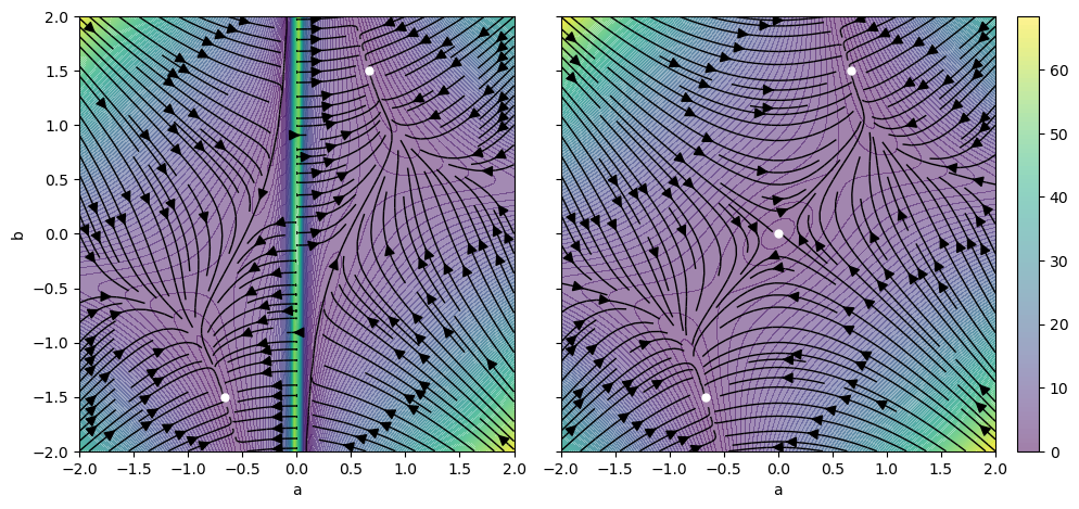
Figure 2: Gradient landscape of $\mathcal{L}^{f^{-1}}$ (left) and $\mathcal{L}^{g}$ (right) for a linear 1D model with $f(x)=ax$, $g(z)=bz$, $q(x)=\mathcal{N}(0,1.5^{2})$ and $\beta=1$. The flow lines show the direction and the contours show the magnitude of the gradient. White dots are critical points. $\mathcal{L}^{g}$ has the same minima $(\pm 2/3,\pm 1.5)$ as $\mathcal{L}^{f^{-1}}$, with an additional critical point at $a=b=0$. This is a saddle, so we will not converge to it in practice. Therefore optimizing $\mathcal{L}^{g}$ results in the same solutions as $\mathcal{L}^{f^{-1}}$.

The following theorem states our main result: that optimizing $\mathcal{L}^{g}$ (eq. 15) is almost equivalent to optimizing $\mathcal{L}^{f^{-1}}$, and that the solutions to $\mathcal{L}^{f^{-1}}$ are maximum likelihood solutions where $p_{\theta}(x)=q(x)$.

Theorem 4.3.

Let $f_{\theta}$ and $g_{\phi}$ be $C^{1}$ and let $f_{\theta}$ be globally invertible. Suppose $q(x)$ is finite and has support everywhere. Then the critical points of $\mathcal{L}^{f^{-1}}$ (for any $\beta>0$) are such that

1. $g_{\phi}(z)=f_{\theta}^{-1}(z)$ for all $z$, and

2. $p_{\theta}(x)=q(x)$ for all $x$, and

3. All critical points are global minima

Furthermore, every minimum of $\mathcal{L}^{f^{-1}}$ is a minimum of $\mathcal{L}^{g}$. If the reconstruction loss is minimal, $\mathcal{L}^{g}$ has no additional critical points.

Note that $\mathcal{L}^{g}$ may have additional critical points if the reconstruction loss is not minimal, meaning that $f_{\theta}$ and $g_{\phi}$ are not globally invertible. An example is when both $f_{\theta}$ and $g_{\phi}$ are the zero function and $q(x)$ has zero mean. We can avoid such solutions by ensuring that $\beta$ is large enough to not tolerate a high reconstruction loss. In the appendix we give guidelines on how to choose $\beta$ is practice.

Figure 2 provides an illuminating example. Here the data and latent space are 1-dimensional and $f$ and $g$ are simple linear functions of a single parameter each. As such we can visualize the gradient landscape in a 2D plot. We see that the additional critical point at the origin is a saddle: there are both converging and diverging gradients. In stochastic gradient descent, it is not plausible that we converge to a saddle since the set of points which converge to it deterministically have measure zero in the parameter space. Hence in this example $\mathcal{L}^{g}$ will converge to the same solutions as $\mathcal{L}^{f^{-1}}$. In addition, it has a smoother gradient landscape (no diverging gradient at $a=0$). While this might not be important in this simple example, in higher dimensions where the Jacobians of adjacent regions could be inconsistent (if the eigenvalues have different signs), it is useful to be able to cross regions where the Jacobian is singular without having to overcome an excessive gradient barrier.

5 EXPERIMENTS

In this section, we demonstrate the practical capabilities of free-form flows (FFF). We mainly compare the performance against normalizing flows based on architectures which are invertible by construction. First, on an inverse problem benchmark, we show that using free-form architectures offers competitive performance to recent spline-based and ODE-based normalizing flows. This is achieved despite minimal tuning of hyperparameters, demonstrating that FFFs are easy to adapt to a new task. Second, on two molecule generation benchmarks, we demonstrate that specialized networks can now be used in a normalizing flow. In particular, we employ the equivariant graph neural networks $E(n)$-GNN (Satorras et al., 2021b, ). This $E(n)$-FFF outperforms ODE-based equivariant normalizing flows in terms of likelihood, and generates stable molecules significantly faster than a diffusion model.

5.1 Simulation-Based Inference

One popular application of generative models is in solving inverse problems. Here, the goal is to estimate hidden parameters from an observation. As inverse problems are typically ambiguous, a probability distribution represented by a generative model is a suitable solution. From a Bayesian perspective, this probability distribution is the posterior of the parameters given the observation. We learn this posterior via a conditional generative model.

In particular, we focus on simulation based inference (SBI, Radev et al., (2020, 2021); Bieringer et al., (2021)), where we want to predict the parameters of a simulation. The training data is parameter, output pairs generated from the simulation.

We train FFF models on the benchmark proposed in (Lueckmann et al.,, 2021), which is comprised of ten inverse problems of varying difficulty at three different simulation budgets (i.e. training-set sizes) each. The models are evaluated via a classifier 2-sample test (C2ST) (Lopez-Paz and Oquab,, 2016; Friedman,, 2003), where a classifier is trained to discern samples from the trained generative model and the true parameter posterior. The model performance is then reported as the classifier accuracy, where 0.5 demonstrates a distribution indistinguishable from the true posterior. We average this accuracy over ten different observations. In fig. 3, we report the C2ST of our model and compare it against the baseline based on neural spline flows (Durkan et al.,, 2019) and flow matching for SBI (Dax et al.,, 2023). Our method performs competitively, especially providing an improvement over existing methods in the regime of low simulation budgets. Regarding tuning of hyperparameters, we find that a simple fully-connected architecture with skip connections works across datasets with minor modifications to increase capacity for the larger datasets. We identify the reconstruction weight $\beta$ large enough such that training becomes stable. We give all dataset and more training details in the appendix.

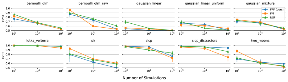
Figure 3: C2ST accuracy on the SBI benchmark datasets. We compare our method (FFF) against flow matching (FM) Dax et al., (2023) and the neural spline flow (NSF) baseline in the benchmark dataset Lueckmann et al., (2021). The accuracy is averaged over ten different observations, with error bars indicating the standard deviation. Our performance is comparable to the competitors across all datasets, with no model being universally better or worse.

5.2 Molecule Generation

Free-form normalizing flows (FFF) do not make any assumptions about the underlying networks $f_{\theta}$ and $g_{\phi}$, except that they preserve dimension. We can leverage this flexibility for tasks where explicit constraints should be built into the architecture, as opposed to constraints that originate from the need for tractable optimization (such as coupling blocks).

As a showcase, we apply FFF to molecule generation. Here, the task is to learn the joint distribution of a number of atoms $x_{1\dots N}\in\mathbb{R}^{n}$. Each prediction of the generative model should yield a physically valid position for each atom: $x=(x_{1},\dots,x_{N})\in\mathbb{R}^{N\times n}$.

The physical system of atoms in space have an important symmetry: if a molecule is shifted or rotated in space, its properties do not change. This means that a generative model for molecules should yield the same probability regardless of orientation and translation:

$$p_{\phi}(Qx+t)\overset{!}{=}p_{\phi}(x).$$ (21)

Here, the rotation $Q\in\mathbb{R}^{3}$ acts on $x$ by rotating or reflecting each atom $x_{i}\in\mathbb{R}^{3}$ about the origin, and $t\in\mathbb{R}^{n}$ applies the same translation to each atom. Formally, $(Q,t)$ are realizations of the Euclidean group $E(n)$. The above eq. 21 means that the distribution $p_{\phi}(x)$ is invariant under the Euclidean group $E(n)$.

Köhler et al., (2020); Toth et al., (2020) showed that if the latent distribution $p(z)$ is invariant under a group $G$, and a generative model $g_{\phi}(z)$ is equivariant to $G$, then the resulting distribution is also invariant to $G$. Equivariance means that applying any group action to the input (e.g. rotation and translation) and then applying $g_{\phi}$ should give the same result as first applying $g_{\phi}$ and then applying the group. For example, for the Euclidean group:

$$Qg_{\phi}(z)+t=g_{\phi}(Qz+t).$$ (22)

This implies that we can learn a distribution invariant to the Euclidean group by construction by making normalizing flows equivariant to the Euclidean group as in eq. 22. Previous work has demonstrated that this inductive bias is more effective than data augmentation, where random rotations and translations are applied to each data point at train time Köhler et al., (2020); Hoogeboom et al., (2022).

We therefore choose an $E(n)$ equivariant network as the networks $f_{\theta}(x)$ and $g_{\phi}(z)$ in our FFF. We employ the $E(n)$-GNN proposed by Satorras et al., 2021b . We call this model the $E(n)$-free-form flow ($E(n)$-FFF).

The $E(n)$-GNN has also been the backbone for previous normalizing flows on molecules. However, to the best of our knowledge, all realizations of such architectures have been based on neural ODEs, where the flow is parameterized as a differential equation $\frac{\mathrm{d}x}{\mathrm{d}t}=f_{\theta}(x(t),t)$. While training, one can avoid solving the ODE by using the rectified flow or flow matching objective (Liu et al.,, 2022; Lipman et al.,, 2022). However, they still have the disadvantage that they require integrating the ODE for sampling.

Boltzmann Generator

We test our $E(n)$-FFFs in learning the Boltzmann distribution:

$$q(x)\propto e^{-\beta u(x)},$$ (23)

where $u(x)\in\mathbb{R}$ is an energy function that takes the positions of atoms $x=(x_{1},\dots,x_{N})$ as an input. A generative model $p_{\phi}(x)$ that approximates $q(x)$ can be used as a Boltzmann generator (Noé et al.,, 2019). The idea of the Boltzmann generator is that having access to $u(x)$ allows re-weighting samples from the generator after training even if $p_{\phi}(x)$ is different from $q(x)$. This is necessary in order to evaluate samples from $q(x)$ in a downstream task: Re-weighting samples allows computing expectation values $\mathbb{E}_{x\sim q(x)}[O(x)]=\mathbb{E}_{x\sim p_{\phi}(x)}[\frac{q(x)}{p_{\phi}(x)}O(x)]$ from samples of the generative model $p_{\phi}(x)$ if $p_{\phi}(x)$ and $q(x)$ have the same support.

We evaluate the performance of free-form flows (FFF) as a Boltzmann generator on the benchmark tasks DW4, LJ13, and LJ55 as presented by Köhler et al., (2020); Klein et al., (2023). Here, pairwise potentials $v(x_{i},x_{j})$ are summed as the total energy $u(x)$:

$$u(x)=\sum_{i,j}v(x_{i},x_{j}).$$ (24)

DW4 uses a double-well potential $v_{\mathtt{DW}}$ and considers four particles in 2D. LJ13 and LJ55 both employ a Lennard-Jones potential $v_{\mathtt{LJ}}$ between 13 respectively 55 particles in 3D space (see appendix for details). We make use of the datasets presented by Klein et al., (2023), which obtained samples from $p(x)$ via MCMC.

In table 1, we compare our model against (i) the equivariant ODE normalizing flow trained with maximum likelihood $E(n)$-NF (Satorras et al., 2021a, ), and (ii) two equivariant ODEs trained via optimal transport (equivariant) flow matching Klein et al., (2023). We find our model to have equal (DW4) or better (LJ13 and LJ55) negative log-likelihood than competitors. In addition, $E(n)$-FFFs sample faster than competitors, even when computing the exact change of variables to evaluate the re-weighting factor of the Boltzmann generator. This is because our model uses $E(n)$-GNNs of similar size to the competitors, but only needs to evaluate them once for sampling, as opposed to the multiple evaluations required to integrate an ODE.

	DW4	LJ13	LJ55
$E(n)$-NF	1.72 $\pm$ 0.01	-16.28 $\pm$ 0.04	n/a
OT-FM	1.70 $\pm$ 0.02	-16.54 $\pm$ 0.03	-94.43 $\pm$ 0.22
E-OT-FM	1.68 $\pm$ 0.01	-16.70 $\pm$ 0.12	-97.93 $\pm$ 0.52
$E(n)$-FFF	1.68 $\pm$ 0.01	-17.09 $\pm$ 0.16	-144.86 $\pm$ 1.42

Table 1: Negative log-likelihood of flow models trained as Boltzmann generators on benchmark datasets. Equivariant free-form flows ($E(n)$-FFF) outperform previous models in terms of negative log-likelihood (NLL, lower is better) on LJ13 and LJ55. The other models are based on an ODE trained via maximum likelihood ($E(n)$-NF, Satorras et al., 2021a ), or trained via Optimal Transport Flow Matching with (OT-FM) or without (E-OT-FM) equivariance-aware matching (Klein et al.,, 2023), and we report the results from Klein et al., (2023). Errors are the standard deviations over runs. $E(n)$-NF is too memory intensive to train on LJ55 efficiently.

QM9 Molecules

As a second molecule generation benchmark, we test the performance of $E(3)$-FFF in generating novel molecules. We therefore train on the QM9 dataset (Ruddigkeit et al.,, 2012; Ramakrishnan et al.,, 2014), which contains molecules of varying atom count, with the largest molecules counting $29$ atoms. The goal of the generative model is not only to predict the positions of the atoms in each molecule $x=(x_{1},\dots,x_{N})\in\mathbb{R}^{3}$, but also each atom’s properties $h_{i}$ (atom type (categorical), and atom charge (ordinal)).

We again employ the $E(3)$-GNN (Satorras et al., 2021b, ). The part of the network that acts on coordinates $x_{i}\in\mathbb{R}^{3}$ is equivariant to rotations, reflections and translations (Euclidean group $E(3)$). The network leaves the atom properties $h$ invariant under these operations. We give the architecture details in the appendix.

We show samples from our model in fig. 1. Because free-form flows only need one network evaluation to sample, they generate two orders of magnitude more stable molecules than the $E(3)$-diffusion model (Hoogeboom et al.,, 2022) and one order of magnitude more than the $E(3)$-normalizing flow (Satorras et al., 2021a, ) in a fixed time window, see table 2. This includes the time to generate unstable samples, which are discarded. A molecule is called stable if each atom has the correct number of bonds, where bonds are determined from inter-atomic distances. $E(3)$-FFF also outperforms $E(3)$-NF trained with maximum likelihood both in terms of likelihood and in how many of the sampled molecules are stable. See appendix for implementation details.

	NLL ($\downarrow$)	Stable ($\uparrow$)	Sampling time ($\downarrow$)
			Raw	Stable
$E(3)$-NF	-59.7	4.9 %	13.9 ms	309.5 ms
$E(3)$-DM	-110.7	82.0 %	1580.8 ms	1970.6 ms
$E(3)$-FFF	-76.2	8.7 %	0.6 ms	8.1 ms
Data	-	95.2 %	-	-

Table 2: $E(3)$-FFF (ours) trained on QM9 generates a stable molecule faster than previous models because a sample is obtained via a single function evaluation. $E(3)$-DM is the $E(3)$-diffusion model (Hoogeboom et al.,, 2022), $E(3)$-NF the $E(3)$-normalizing flow (Satorras et al., 2021a, ). The latter is also trained explicitly using maximum likelihood, yet outperformed by $E(3)$-FFF in terms of negative log-likelihood (NLL) and what ratio of generated molecules is stable.

6 CONCLUSION

In this work, we present free-form flows (FFF), a new paradigm for normalizing flows that enables training arbitrary dimension-preserving neural networks with maximum likelihood. Invertibility is achieved by a reconstruction loss and the likelihood is maximized by an efficient surrogate. Previously, designing normalizing flows was constrained by the need for analytical invertibility. Free-form flows allow practitioners to focus on the data and suitable inductive biases instead.

We show that free-form flows are an exact relaxation of maximum likelihood training, converging to the same solutions provided that the reconstruction loss is minimal. We provide an interpretation of FFF training as the minimization of a lower bound on the KL divergence between noisy versions of the data and the generative distribution. Furthermore this bound is tight if $f_{\theta}$ and $g_{\phi}$ are true inverses.

In practice, free-form flows perform on par or better than previous normalizing flows, exhibit fast sampling and are easy to tune.

Acknowledgments

This work is supported by Deutsche Forschungsgemeinschaft (DFG, German Research Foundation) under Germany’s Excellence Strategy EXC-2181/1 - 390900948 (the Heidelberg STRUCTURES Cluster of Excellence). It is also supported by the Vector Stiftung in the project TRINN (P2019-0092). AR acknowledges funding from the Carl-Zeiss-Stiftung. LZ ackknowledges support by the German Federal Ministery of Education and Research (BMBF) (project EMUNE/031L0293A). The authors acknowledge support by the state of Baden-Württemberg through bwHPC and the German Research Foundation (DFG) through grant INST 35/1597-1 FUGG.

 

Supplementary Materials

 

OVERVIEW

The appendix is structured into three parts:

• Section 7: A restatement and proof of all theoretical claims in the main text, along with some additional results.

  • Section 7.1: The gradient of the log-determiant can be written as a trace.

  • Section 7.2: A derivation of the loss as a lower bound on a KL divergence.

  • Section 7.3: A bound on the difference between the true gradient of the log-determinant and the estimator used in this work.

  • Section 7.4: Properties of the critical points of the loss.

  • Section 7.5: Exploration of behavior of the loss in the low $\beta$ regime, where the solution may not be globally invertible.

• Section 8: Practical tips on how to train free-form flows and adapt them to new problems.

  • Section 8.1: Tips on how to set up and initialize the model.

  • Section 8.2: Code for computing the loss function.

  • Section 8.3: Details on how to estimate likelihoods.

  • Section 8.4: Tips on how to tune $\beta$.

• Section 9: Details necessary to reproduce all experimental results in the main text.

  • Section 9.1: Simulation-based inference.

  • Section 9.2: Molecule generation.

7 THEORETICAL CLAIMS

This section contains restatements and proofs of all theoretical claims in the main text.

7.1 Gradient via Trace

Theorem 7.1.

Let $f_{\theta}:\mathbb{R}^{D}\to\mathbb{R}^{D}$ be a $C^{1}$ invertible function parameterized by $\theta$. Then, for all $x\in\mathbb{R}^{D}$:

$$\nabla_{\theta_{i}}\log|J_{\theta}(x)|=\operatorname{tr}\!\left((J_{\theta}(x))^{-1}\nabla_{\theta_{i}}J_{\theta}(x)\right).$$ (25)

Proof.

Jacobi’s formula states that, for a matrix $A(t)$ parameterized by $t$, the derivative of the determinant is

$$\frac{\mathrm{d}}{\mathrm{d}t}|A(t)|=|A(t)|\operatorname{tr}\left(A(t)^{-1}\frac{\mathrm{d}A(t)}{\mathrm{d}t}\right)$$ (26)

and hence

$$\frac{\mathrm{d}}{\mathrm{d}t}\log|A(t)| =|A(t)|^{-1}\frac{\mathrm{d}}{\mathrm{d}t}|A(t)|$$ (27)

$$=\operatorname{tr}\left(A(t)^{-1}\frac{\mathrm{d}A(t)}{\mathrm{d}t}\right)$$ (28)

Applying this formula, with $A=J_{\theta}(x)$ and $t=\theta_{i}$ gives the result. ∎

7.2 Loss Derivation

Here we derive the loss function via an upper bound on a Kullback-Leibler (KL) divergence. Before doing so, let us establish some notation and motivation.

Our generative model is as follows:

$$p(z) =\mathcal{N}(z;0,I)$$ (29)

$$p_{\phi}(x\mid z) =\delta(x-g_{\phi}(z))$$ (30)

meaning that to generate data we sample from a standard normal latent distribution and pass the sample through the generator network $g_{\phi}$. The corresponding inference model is:

$$q(x) =\text{data distribution}$$ (31)

$$q_{\theta}(z\mid x) =\delta(z-f_{\theta}(x))$$ (32)

Our goal is to minimize the KL divergence

$$\mathcal{D}_{\text{KL}}(q(x)\parallel p_{\phi}(x)) =\mathbb{E}_{q(x)}\left[\log\frac{q(x)}{p_{\phi}(x)}\right]$$ (33)

$$=\mathbb{E}_{q(x)}\left[-\log\int p_{\phi}(x,z)\mathrm{d}z\right]-h(q(x))$$ (34)

where $h$ denotes the differential entropy. Unfortunately this divergence is intractable, due to the integral over $z$ (though it would be tractable if $g_{\phi}^{-1}$ and $\log|J_{g_{\phi}}(z)|$ are tractable due to the change of variables formula – in this case the model would be a typical normalizing flow). The variational autoencoder (VAE) is a latent variable model which solves this problem by minimizing

$$\mathcal{D}_{\text{KL}}(q_{\theta}(x,z)\parallel p_{\phi}(x,z)) =E_{q_{\theta}(x,z)}\left[\log\frac{q_{\theta}(x,z)}{p_{\phi}(x,z)}\right]$$ (35)

$$=E_{q_{\theta}(x,z)}\left[\log\frac{q(x)}{p_{\phi}(x)}+\log\frac{q_{\theta}(z\mid x)}{p_{\phi}(z\mid x)}\right]$$ (36)

$$=\mathcal{D}_{\text{KL}}(q(x)\parallel p_{\phi}(x))+E_{q(x)}\left[\mathcal{D}_{\text{KL}}(q_{\theta}(z\mid x)\parallel p_{\phi}(z\mid x))\right]$$ (37)

$$\geq\mathcal{D}_{\text{KL}}(q(x)\parallel p_{\phi}(x))$$ (38)

The inequality comes from the fact that KL divergences are always non-negative. Unfortunately this KL divergence is not well-defined due to the delta distributions, which make the joint distributions over $x$ and $z$ degenerate. Unless the support of $q_{\theta}(x,z)$ and $p_{\phi}(x,z)$ exactly overlap, which is very unlikely for arbitrary $f_{\theta}$ and $g_{\phi}$, the divergence will be infinite. The solution is to introduce an auxiliary variable $\tilde{x}$ which is the data with some added Gaussian noise:

$$p(\tilde{x}\mid x)=q(\tilde{x}\mid x)=\mathcal{N}(\tilde{x};x,\sigma^{2}I)$$ (39)

The generative model over $z$ and $\tilde{x}$ is therefore

$$p(z) =\mathcal{N}(z;0,I)$$ (40)

$$p_{\phi}(\tilde{x}\mid z) =\mathcal{N}(\tilde{x};g_{\phi}(z),\sigma^{2}I)$$ (41)

and the inference model is

$$q(\tilde{x}) =\int q(x)q(\tilde{x}\mid x)\mathrm{d}x$$ (42)

$$q(\tilde{x}\mid x) =\mathcal{N}(\tilde{x};x,\sigma^{2}I)$$ (43)

$$q_{\theta}(z\mid\tilde{x}) =\frac{\int q(x)q(\tilde{x}\mid x)q_{\theta}(z\mid x)\mathrm{d}x}{\int q(x)q(\tilde{x}\mid x)\mathrm{d}x}$$ (44)

Now the relationship between $\tilde{x}$ and $z$ is stochastic and we can safely minimize the KL divergence which will always take on finite values:

$$\mathcal{D}_{\text{KL}}(q_{\theta}(\tilde{x},z)\parallel p_{\phi}(\tilde{x},z))\geq\mathcal{D}_{\text{KL}}(q(\tilde{x})\parallel p_{\phi}(\tilde{x}))$$ (45)

For convenience, here is the definition of $\mathcal{L}^{f^{-1}}$:

$$\mathcal{L}^{f^{-1}}=\mathbb{E}_{q(x)}\left[-\log p(Z=f_{\theta}(x))-\operatorname{tr}(\texttt{SG}(v^{T}J_{\theta}^{-1})J_{\theta}v)+\beta\lVert x-g_{\phi}(f_{\theta}(x))\rVert^{2}\right]$$ (46)

with the property (see main text)

$$\mathbb{E}_{v}[\mathcal{L}^{f^{-1}}]=\mathbb{E}_{q(x)}\left[-\log p(Z=f_{\theta}(x))-\log|J_{\theta}|+\beta\lVert x-g(f(x))\rVert^{2}\right]$$ (47)

Now we restate the theorem from the main text:

Theorem 7.2.

Let $f_{\theta}$ and $g_{\phi}$ be $C^{1}$ and let $f_{\theta}$ be globally invertible. Add isotropic Gaussian noise of variance $\sigma^{2}$ to both the data distribution and generated distribution to obtain $q(\tilde{x})$ and $p_{\phi}(\tilde{x})$ respectively. Let $\beta=1/2\sigma^{2}$. Then there exists a function $D$ of $\theta$ and $\phi$ such that

$$\nabla_{\theta}\mathbb{E}_{v}[\mathcal{L}^{f^{-1}}]=\nabla_{\theta}D\quad\text{and}\quad\nabla_{\phi}\mathbb{E}_{v}[\mathcal{L}^{f^{-1}}]=\nabla_{\phi}D$$ (48)

and

$$D\geq\mathcal{D}_{\text{KL}}(q(\tilde{x})\parallel p_{\phi}(\tilde{x}))$$ (49)

As a result, minimizing $\mathcal{L}^{f^{-1}}$ is equivalent to minimizing an upper bound on $\mathcal{D}_{\text{KL}}(q(\tilde{x})\parallel p_{\phi}(\tilde{x}))$.

Proof.

Let

$$D=\mathcal{D}_{\text{KL}}(q_{\theta}(\tilde{x},z)\parallel p_{\phi}(\tilde{x},z))$$ (50)

We will use the identity (Papoulis and Pillai,, 2002)

$$h(Z)=h(X)+\mathbb{E}[\log|J_{f}(X)|]$$ (51)

where $h$ is the differential entropy, and the random variables are related by $Z=f(X)$ where $f$ is invertible. As a result,

$$h(q(z\mid\tilde{x}))=h(q(x\mid\tilde{x}))+\mathbb{E}_{q(x\mid\tilde{x})}[\log|J_{f}(x)|]=\mathbb{E}_{q(x)}[\log|J_{f}(x)|]+\text{const.}$$ (52)

In the following, drop $\theta$ and $\phi$ subscripts for convenience. The unspecified extra terms are constant with respect to network parameters. Let $\epsilon$ be a standard normal variable. Then:

$$D =\mathbb{E}_{q(\tilde{x},z)}\left[\log q(\tilde{x})+\log q(z\mid\tilde{x})-\log p(z)-\log p(\tilde{x}\mid z)\right]$$ (53)

$$=\mathbb{E}_{q(\tilde{x})}\left[-h(q(z\mid\tilde{x}))\right]+\mathbb{E}_{q(\tilde{x},z)}\left[-\log p(z)-\log p(\tilde{x}\mid z)\right]+\text{const.}$$ (54)

$$=\mathbb{E}_{q(x)}\left[-\log|J_{f}(x)|\right]+\mathbb{E}_{q(\tilde{x},z)}\left[-\log p(z)-\log p(\tilde{x}\mid z)\right]+\text{const.}$$ (55)

$$=\mathbb{E}_{q(x)q(\epsilon)}\left[-\log|J_{f}(x)|-\log p(Z=f(x))-\log p(\tilde{X}=x+\sigma\epsilon\mid Z=f(x))\right]+\text{const.}$$ (56)

$$=\mathbb{E}_{q(x)q(\epsilon)}\left[-\log|J_{f}(x)|-\log p(Z=f(x))+\frac{1}{2\sigma^{2}}\lVert x+\sigma\epsilon-g(f(x))\rVert^{2}\right]+\text{const.}$$ (57)

$$=\mathbb{E}_{q(x)q(\epsilon)}\left[-\log|J_{f}(x)|-\log p(Z=f(x))+\frac{1}{2\sigma^{2}}\lVert x-g(f(x))\rVert^{2}+\frac{1}{\sigma}\epsilon^{\top}(x-g(f(x)))\right]+\text{const.}$$ (58)

$$=\mathbb{E}_{q(x)}\left[-\log|J_{f}(x)|-\log p(Z=f(x))+\beta\lVert x-g(f(x))\rVert^{2}\right]+\text{const.}$$ (59)

$$=\mathbb{E}_{v}[\mathcal{L}^{f^{-1}}]+\text{const.}$$ (60)

Where the following steps were taken:

• Regard $\mathbb{E}_{q(\tilde{x})}[\log q(\tilde{x})]=-h(q(\tilde{x}))$ as a constant (eq. 54)

• Substitute in eq. 52 and regard $h(q(x\mid\tilde{x}))$ as constant (eq. 55)

• Make a change of variables from $\tilde{x},z$ to $x,\epsilon$ with $\tilde{x}=x+\sigma\epsilon$ and $z=f(x)$ (eq. 56)

• Substitute the log-likelihood of the Gaussian $p(\tilde{x}\mid z)$, discard constant terms (eq. 57)

• Expand the final quadratic term, discard the constant term in $\lVert\epsilon\rVert^{2}$ (eq. 58)

• Evaluate the expectation over $\epsilon$, noting that $\epsilon$ is independent of $x$ and $\mathbb{E}[\epsilon]=0$. Substitute $\beta=1/2\sigma^{2}$ (eq. 59)

• Recognize $\mathcal{L}^{f^{-1}}$ from eq. 46 (eq. 60)

Since the extra terms are constant with respect to $\theta$ and $\phi$ we have

$$\nabla_{\theta}\mathbb{E}_{v}[\mathcal{L}^{f^{-1}}]=\nabla_{\theta}D\quad\text{and}\quad\nabla_{\phi}\mathbb{E}_{v}[\mathcal{L}^{f^{-1}}]=\nabla_{\phi}D$$ (61)

and

$$D\geq\mathcal{D}_{\text{KL}}(q(\tilde{x})\parallel p_{\phi}(\tilde{x}))$$ (62)

was already established. As a result the gradients of $\mathcal{L}^{f^{-1}}$ are an unbiased estimate of the gradients of $D$ and minimizing $\mathcal{L}^{f^{-1}}$ under stochastic gradient descent will converge to the same solutions as when minimizing $D$.

∎

7.3 Error Bound

Theorem 7.3.

Let $f_{\theta}$ and $g_{\phi}$ be $C^{1}$, let $J_{\theta}$ be the Jacobian of $f_{\theta}$ at $x$ and let $J_{\phi}$ be the Jacobian of $g_{\phi}$ at $f_{\theta}(x)$. Suppose that $f_{\theta}$ is locally invertible at $x$, meaning $J_{\theta}(x)$ is an invertible matrix. Let $\lVert\cdot\rVert_{F}$ be the Frobenius norm of a matrix. Then the absolute difference between $\nabla_{\theta_{i}}\log|J_{\theta}(x)|$ and the trace-based approximation is bounded:

$$\left|\operatorname{tr}(J_{\phi}\nabla_{\theta_{i}}J_{\theta})-\nabla_{\theta_{i}}\log|J_{\theta}|\right|\leq\lVert J_{\theta}^{-1}\nabla_{\theta_{i}}J_{\theta}\rVert_{F}\lVert J_{\phi}J_{\theta}-I\rVert_{F}$$ (63)

Proof.

The Cauchy-Schwarz inequality states that, for an inner product $\langle\cdot,\cdot\rangle$

$$|\langle u,v\rangle|^{2}\leq\langle u,u\rangle\langle v,v\rangle$$ (64)

The trace forms the so-called Frobenius inner product over matrices with $\langle A,B\rangle_{F}=\operatorname{tr}(A^{T}B)$. Applying the inequality gives

$$|\operatorname{tr}(A^{T}B)|^{2} \leq\operatorname{tr}(A^{T}A)\operatorname{tr}(B^{T}B)$$ (65)

$$=\lVert A\rVert_{F}^{2}\lVert B\rVert_{F}^{2}$$ (66)

with $\lVert A\rVert_{F}=\sqrt{\operatorname{tr}(A^{T}A)}$ the Frobenius norm of $A$.

Recall from theorem 7.1 that

$$\nabla_{\theta_{i}}\log|J_{\theta}|=\operatorname{tr}(J_{\theta}^{-1}\nabla_{\theta_{i}}J_{\theta})$$ (67)

Therefore

$$\left|\operatorname{tr}(J_{\phi}\nabla_{\theta_{i}}J_{\theta})-\nabla_{\theta_{i}}\log|J_{\theta}|\right| =\left|\operatorname{tr}(J_{\phi}\nabla_{\theta_{i}}J_{\theta})-\operatorname{tr}(J_{\theta}^{-1}\nabla_{\theta_{i}}J_{\theta})\right|$$ (68)

$$=\left|\operatorname{tr}((J_{\phi}-J_{\theta}^{-1})\nabla_{\theta_{i}}J_{\theta})\right|$$ (69)

$$=\left|\operatorname{tr}((J_{\phi}J_{\theta}-I)J_{\theta}^{-1}\nabla_{\theta_{i}}J_{\theta})\right|$$ (70)

$$\leq\lVert J_{\theta}^{-1}\nabla_{\theta_{i}}J_{\theta}\rVert_{F}\lVert J_{\phi}J_{\theta}-I\rVert_{F}$$ (71)

where the last line is application of the Cauchy-Schwarz inequality. ∎

Theorem 7.4.

Suppose the conditions of theorem 7.3 hold but extend local invertibility of $f_{\theta}$ to invertibility wherever $q(x)$ has support. Then the difference in gradients between $\mathcal{L}^{g}$ and $\mathcal{L}^{f^{-1}}$ is bounded:

$$\left|\nabla_{\theta_{i}}\mathbb{E}_{v}[\mathcal{L}^{g}]-\nabla_{\theta_{i}}\mathbb{E}_{v}[\mathcal{L}^{f^{-1}}]\right|\leq\mathbb{E}_{q(x)}\left[\lVert J_{\theta}^{-1}\nabla_{\theta_{i}}J_{\theta}\rVert_{F}^{2}\right]^{\frac{1}{2}}\mathbb{E}_{q(x)}\left[\lVert J_{\phi}J_{\theta}-I\rVert_{F}^{2}\right]^{\frac{1}{2}}$$ (72)

Proof.

In addition to the Cauchy-Schwarz inequality used in the proof to theorem 7.3, we will also require Jensen’s inequality for a convex function $\alpha:\mathbb{R}\rightarrow\mathbb{R}$

$$\alpha(\mathbb{E}_{q(x)}[x])\leq\mathbb{E}_{q(x)}[\alpha(x)]$$ (73)

and Hölder’s inequality (with $p=q=2$) for random variables $X$ and $Y$

$$\mathbb{E}[|XY|]\leq\mathbb{E}[|X|^{2}]^{\frac{1}{2}}\mathbb{E}[|Y|^{2}]^{\frac{1}{2}}$$ (74)

The only difference between $\mathcal{L}^{g}$ and $\mathcal{L}^{f^{-1}}$ is in the estimation of the gradient of the log-determinant. We use this fact, along with the inequalities, which we apply in the Jensen, Cauchy-Schwarz, Hölder order:

$$\left|\nabla_{\theta_{i}}\mathbb{E}_{v}[\mathcal{L}^{g}]-\nabla_{\theta_{i}}\mathbb{E}_{v}[\mathcal{L}^{f^{-1}}]\right| =\left|\mathbb{E}_{q(x)}\left[\operatorname{tr}(J_{\phi}\nabla_{\theta_{i}}J_{\theta})\right]-\mathbb{E}_{q(x)}\left[\nabla_{\theta_{i}}\log|J_{\theta}|\right]\right|$$ (75)

$$=\left|\mathbb{E}_{q(x)}\left[\operatorname{tr}((J_{\phi}J_{\theta}-I)J_{\theta}^{-1}\nabla_{\theta_{i}}J_{\theta})\right]\right|$$ (76)

$$\leq\mathbb{E}_{q(x)}\left[\left|\operatorname{tr}((J_{\phi}J_{\theta}-I)J_{\theta}^{-1}\nabla_{\theta_{i}}J_{\theta})\right|\right]$$ (77)

$$\leq\mathbb{E}_{q(x)}\left[\lVert J_{\theta}^{-1}\nabla_{\theta_{i}}J_{\theta}\rVert_{F}\lVert J_{\phi}J_{\theta}-I\rVert_{F}\right]$$ (78)

$$\leq\mathbb{E}_{q(x)}\left[\lVert J_{\theta}^{-1}\nabla_{\theta_{i}}J_{\theta}\rVert_{F}^{2}\right]^{\frac{1}{2}}\mathbb{E}_{q(x)}\left[\lVert J_{\phi}J_{\theta}-I\rVert_{F}^{2}\right]^{\frac{1}{2}}$$ (79)

∎

7.4 Critical Points

Theorem 7.5.

Let $f_{\theta}$ and $g_{\phi}$ be $C^{1}$ and let $f_{\theta}$ be globally invertible. Suppose $q(x)$ is finite and has support everywhere. Then the critical points of $\mathcal{L}^{f^{-1}}$ (for any $\beta>0$) are such that

1. $g_{\phi}(z)=f_{\theta}^{-1}(z)$ for all $z$, and

2. $p_{\theta}(x)=q(x)$ for all $x$, and

3. All critical points are global minima

Furthermore, every minimum of $\mathcal{L}^{f^{-1}}$ is a minimum of $\mathcal{L}^{g}$. If the reconstruction loss is minimal, $\mathcal{L}^{g}$ has no additional critical points.

Proof.

In the following we will use Einstein notation, meaning that repeated indices are summed over. For example, $a_{i}b_{i}$ is shorthand for $\sum_{i}a_{i}b_{i}$. We will drop $\theta$ and $\phi$ subscripts to avoid clutter. We will also use primes to denote derivatives, for example: $f^{\prime}(x)=J_{f}(x)$. In addition, gradients with respect to parameters should be understood as representing the gradient of a single parameter at a time, so $\nabla_{\theta}\mathcal{L}$ is shorthand for $(\nabla_{\theta_{1}}\mathcal{L},\dots)$.

Let $\mathcal{L}=\mathbb{E}_{v}[\mathcal{L}^{f^{-1}}]$.

We will use the calculus of variations to find the critical points on a functional level. For a primer on calculus of variations, please see Weinstock, (1974). Our loss is of the form

$$\mathcal{L}=\int\lambda(x,f,f^{\prime},g)\mathrm{d}x$$ (80)

with

$$\lambda(x,f,f^{\prime},g)=q(x)\left(\frac{1}{2}\lVert f(x)\rVert^{2}-\log|f^{\prime}(x)|+\beta\lVert g(f(x))-x\rVert^{2}\right)$$ (81)

By the Euler-Lagrange equations, critical points satisfy

$$\frac{\partial\lambda}{\partial g_{i}}=0$$ (82)

for all $i$ and

$$\frac{\partial\lambda}{\partial f_{i}}-\frac{\partial}{\partial x_{j}}\left(\frac{\partial\lambda}{\partial f^{\prime}_{ij}}\right)=0$$ (83)

for all $i$.

Taking the derivative with respect to $g$:

$$\frac{\partial\lambda}{\partial g_{i}}=q(x)\cdot 2\beta(g(f(x))-x)_{i}=0$$ (84)

and hence $g(f(x))-x=0$ for all $x$ (since $q(x)>0$). By a change of variables with $z=f(x)$, this means $g=f^{-1}$. Therefore we have proven statement 1.

Now differentiating with respect to $f$ and substituting $g=f^{-1}$:

$$\frac{\partial\lambda}{\partial f_{i}} =q(x)\left(f_{i}(x)+2\beta(g(f(x))-x)_{j}g^{\prime}_{ji}(f(x))\right)$$ (85)

$$=q(x)f_{i}(x)$$ (86)

and with respect to $f^{\prime}$:

$$\frac{\partial\lambda}{\partial f^{\prime}_{ij}} =-q(x)(f^{\prime}(x)^{-1})_{lk}\frac{\partial f^{\prime}_{kl}}{\partial f^{\prime}_{ij}}$$ (87)

$$=-q(x)(f^{\prime}(x)^{-1})_{ji}$$ (88)

meaning

$$\frac{\partial}{\partial x_{j}}\left(\frac{\partial\lambda}{\partial f^{\prime}_{ij}}\right) =-\frac{\partial}{\partial x_{j}}q(x)(f^{\prime}(x)^{-1})_{ji}-q(x)\frac{\partial}{\partial x_{j}}(f^{\prime}(x)^{-1})_{ji}$$ (89)

$$=-q(x)\left(\frac{\partial}{\partial x_{j}}\log q(x)(f^{\prime}(x)^{-1})_{ji}+\frac{\partial}{\partial x_{j}}(f^{\prime}(x)^{-1})_{ji}\right)$$ (90)

Putting it together means

$$q(x)\left(f_{i}(x)+\frac{\partial}{\partial x_{j}}\log q(x)(f^{\prime}(x)^{-1})_{ji}+\frac{\partial}{\partial x_{j}}(f^{\prime}(x)^{-1})_{ji}\right)=0$$ (91)

By dividing by $q(x)$ and multiplying by $f^{\prime}_{ik}(x)$, we have

$$\frac{\partial}{\partial x_{k}}\log q(x)=-f_{i}(x)f^{\prime}_{ik}(x)-\frac{\partial}{\partial x_{j}}(f^{\prime}(x)^{-1})_{ji}f^{\prime}_{ik}(x)$$ (92)

Furthermore, since $f(x)$ is invertible:

$$\frac{\partial}{\partial x_{j}}\left(f^{\prime}(x)^{-1}f^{\prime}(x)\right)_{jk}=\frac{\partial}{\partial x_{j}}\delta_{jk}=0$$ (93)

Then using the product rule:

$$\frac{\partial}{\partial x_{j}}(f^{\prime}(x)^{-1})_{ji}f^{\prime}_{ik}(x)+(f^{\prime}(x)^{-1})_{ji}f^{\prime\prime}_{ikj}(x)=0$$ (94)

In addition,

$$\frac{\partial}{\partial x_{k}}\log|f^{\prime}(x)|=(f^{\prime}(x)^{-1})_{ji}f^{\prime\prime}_{ijk}(x)$$ (95)

from Jacobi’s formula, and since Hessians are symmetric in their derivatives, we can put together eq. 94 and eq. 95 to form

$$\frac{\partial}{\partial x_{j}}(f^{\prime}(x)^{-1})_{ji}f^{\prime}_{ik}(x)=-\frac{\partial}{\partial x_{k}}\log|f^{\prime}(x)|$$ (96)

Substituting into eq. 92 and integrating, we find

$$\log q(x)=-\frac{1}{2}\lVert f(x)\rVert^{2}+\log|f^{\prime}(x)|+\text{const.}$$ (97)

The RHS is $\log p_{\theta}(x)$ by the change of variables formula, and hence $p_{\theta}(x)=q(x)$ for all $x$. This proves statement 2.

Now we will show that all critical points are global minima.

The negative log-likelihood part of $\mathcal{L}$ is bounded below by $h(q(x))$ and the reconstruction part is bounded below by zero. Hence if all critical points achieve a loss of $h(q(x))$ they are all global minima.

Since $g=f^{-1}$ for all critical points, the reconstruction loss is zero.

Since $p_{\theta}(x)=q(x)$ for all critical points, the negative log-likelihood loss is $h(q(x))$:

$$\mathbb{E}_{q(x)}[-\log p_{\theta}(x)]=\mathbb{E}_{q(x)}[-\log q(x)]=h(q(x))$$ (98)

This proves statement 3.

It now remains to show that every minimum of $\mathcal{L}^{f^{-1}}$ is a minimum of $\mathcal{L}^{g}$.

Let $\tilde{\mathcal{L}}=\mathbb{E}_{v}[\mathcal{L}^{g}]$. This means that

$$\tilde{\mathcal{L}}=\int\tilde{\lambda}(x,f,f^{\prime},g)\mathrm{d}x$$ (99)

with

$$\tilde{\lambda}(x,f,f^{\prime},g)=q(x)\left(\frac{1}{2}\lVert f(x)\rVert^{2}-\operatorname{tr}(\texttt{SG}(g^{\prime}(f(x)))f^{\prime}(x))+\beta\lVert g(f(x))-x\rVert^{2}\right)$$ (100)

$$\frac{\partial\tilde{\lambda}}{\partial g_{i}}=q(x)\cdot 2\beta(g(f(x))-x)_{i}$$ (101)

as before, and is zero with the substitution $g=f^{-1}$.

$$\frac{\partial\tilde{\lambda}}{\partial f_{i}}=q(x)f_{i}(x)$$ (102)

as before and

$$\frac{\partial\tilde{\lambda}}{\partial f^{\prime}_{ij}} =-q(x)g^{\prime}_{lk}(f(x))\frac{\partial f^{\prime}_{kl}}{\partial f^{\prime}_{ij}}$$ (103)

$$=-q(x)g^{\prime}_{ji}(f(x))$$ (104)

$$=-q(x)(f^{\prime}(x)^{-1})_{ji}$$ (105)

with the substitution $g^{\prime}(f(x))=f^{\prime}(x)^{-1}$. Since this is the same expression as before we must have

$$\frac{\partial\tilde{\lambda}}{\partial f_{i}}-\frac{\partial}{\partial x_{j}}\left(\frac{\partial\tilde{\lambda}}{\partial f^{\prime}_{ij}}\right)=0$$ (106)

meaning that $f$ and $g$ are critical with respect to $\tilde{\mathcal{L}}$. This shows that the critical points of $\mathcal{L}^{f^{-1}}$ are critical points of $\mathcal{L}^{g}$.

In the case where $f$ is not required to be globally invertible, $\mathcal{L}^{g}$ may have additional critical points when $f$ is in fact not invertible. However, if the reconstruction loss is minimal, therefore zero, $f$ will be invertible and the above arguments hold. If this is the case, there are no additional critical points of $\mathcal{L}^{g}$.

∎

7.5 Ensuring Global Invertibility

Free-form flows use arbitrary neural networks $f_{\theta}$ and $g_{\phi}$. Since we rely on the approximation $g_{\phi}\approx f_{\theta}^{-1}$, it is crucial that the reconstruction loss is as small as possible. We achieve this in practice by setting $\beta$ large enough. In this section, we give the reasoning for this choice.

In particular, we show that when $\beta$ is too small and the data is made up of multiple disconnected components, there are solutions to $\mathcal{L}^{f^{-1}}$ that are not globally invertible, even if $f_{\theta}$ is restricted to be locally invertible. We illustrate some of these solutions for a two-component Gaussian mixture in fig. 4. We approximate the density as zero more than 5 standard deviations away from each mean. When $\beta$ is extremely low the model gives up on reconstruction and just tries to transform each component to the latent distribution individually.

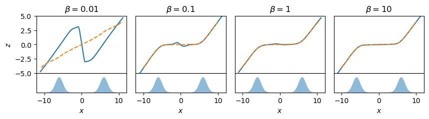
Figure 4: Solutions to $\mathcal{L}^{f^{-1}}$ for various $\beta$. The data is the two-component Gaussian mixture shown in the lower panels. Solid blue lines show $f_{\theta}$ and dashed orange lines show $g_{\phi}$. Note that $f_{\theta}$ is not invertible between the mixtures when $\beta$ is small.

Let us now analyse the behavior of this system mathematically. Our argument goes as follows: First, we assume that the data can be split into disconnected regions. Then it might be favorable that the encoder computes latent codes such that each region covers the full latent space. This means that each latent code $z$ is assigned once in each region. This is a valid encoder function $f_{\theta}$ and we compute its loss $\mathcal{L}^{f^{-1}}$ in theorem 7.6. In corollary 7.6.1, we show that when $\beta<\beta_{\text{crit}}$ solutions which are not globally invertible have the lowest loss. It is thus vital that $\beta>\beta_{\text{crit}}$ or larger to ensure the solution is globally invertible.

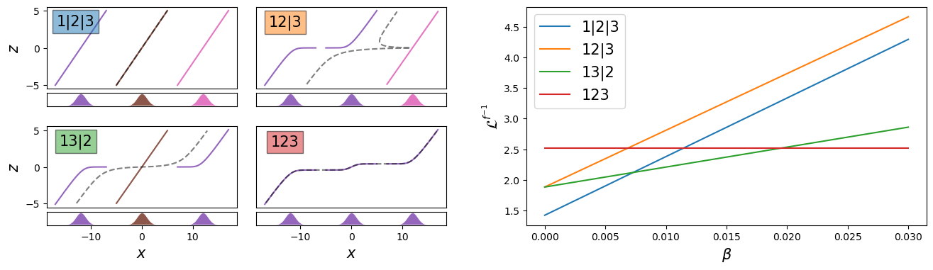
Figure 5: Intuition behind theorem 7.6: Comparison of invalid solutions to learning a Gaussian mixture of three modes with non-invertible encoders (blue, orange, green), compared to an invertible encoder (red). (Left) As the encoder is not invertible by construction, it may learn to reuse each latent code $z$ once for each disconnected component. This reduces the negative-likelihood at each point, as the derivative $f_{\theta}^{\prime}(x)$ is larger at each data point. The decoder (dotted gray line) then cannot reconstruct the data. (Right) Increasing $\beta$ increases the importance of reconstruction over maximum likelihood and thus selects the best solution (red).

Theorem 7.6.

Let $f_{\theta}$ and $g_{\phi}$ be $C^{1}$. Suppose that $q(x)$ may not have support everywhere and allow $f_{\theta}$ to be non-invertible in the regions where $q(x)=0$. Suppose the set $\mathcal{S}=\{x:q(x)>0\}$ is made up of $k$ disjoint, connected components: $\mathcal{S}=\bigcup_{i=1}^{k}\mathcal{S}_{i}$.

For each partition $\mathcal{P}$ of $\{\mathcal{S}_{i}\}_{i=1}^{k}$ consider solutions of $\mathcal{L}^{f^{-1}}$ where

1. $f_{\theta}$ transforms each element of the partition to $p(z)$ individually, and

2. $g_{\phi}$ is chosen (given $f_{\theta}$) such that $R_{\min}=\mathbb{E}_{x}\left[\lVert g_{\phi}(f_{\theta}(x))-x\rVert^{2}\right]$ is minimal

The loss achieved is

$$\mathcal{L}^{f^{-1}}=h(q(x))-H(\mathcal{P})+\beta R_{\min}(\mathcal{P})$$ (107)

where $h(q(x))$ is the differential entropy of the data distribution and $H(\mathcal{P})$ is the entropy of $\alpha$ where $\alpha_{i}=\int_{\mathcal{P}_{i}}q(x)\mathrm{d}x$.

Note that the solutions in theorem 7.6 are not necessarily minima of $\mathcal{L}^{f^{-1}}$, they just demonstrate what values it can take.

Proof.

Let $\mathcal{L}=\mathbb{E}_{v}[\mathcal{L}^{f^{-1}}]$. The loss can be split into negative log-likelihood and reconstruction parts: $\mathcal{L}=\mathcal{L}_{\text{NLL}}+\beta\mathcal{L}_{\text{R}}$.

Consider a partition $\mathcal{P}$ of $\{\mathcal{S}_{i}\}_{i=1}^{k}$. Let $q_{i}(x)$ be the distribution which is proportional to $q(x)$ when $x\in\mathcal{P}_{i}$ but zero otherwise (weighted to integrate to 1):

$$q_{i}(x)=\frac{1}{\alpha_{i}}q(x)1\!\!1_{x\in\mathcal{P}_{i}}$$ (108)

with

$$\alpha_{i}=\int_{\mathcal{P}_{i}}q(x)\mathrm{d}x$$ (109)

The type of solution described in the theorem statement will be such that $p_{\theta}(x)=q_{i}(x)$ for $x\in\mathcal{P}_{i}$. This means that

$$\mathcal{L}_{\text{NLL}} =-\int q(x)\log p_{\theta}(x)\mathrm{d}x$$ (110)

$$=-\sum_{i}\int_{\mathcal{P}_{i}}q(x)\log p_{\theta}(x)\mathrm{d}x$$ (111)

$$=-\sum_{i}\alpha_{i}\int_{\mathcal{P}_{i}}q_{i}(x)\log q_{i}(x)\mathrm{d}x$$ (112)

$$=\sum_{i}\alpha_{i}h(q_{i}(x))$$ (113)

We also have

$$h(q(x)) =-\sum_{i}\int_{\mathcal{P}_{i}}q(x)\log q(x)\mathrm{d}x$$ (114)

$$=-\sum_{i}\alpha_{i}\int_{\mathcal{P}_{i}}q_{i}(x)\log(\alpha_{i}q_{i}(x))\mathrm{d}x$$ (115)

$$=\sum_{i}\alpha_{i}\left(h(q_{i}(x))-\log\alpha_{i}\right)$$ (116)

$$=\mathcal{L}_{\text{NLL}}+H(\alpha)$$ (117)

and therefore

$$\mathcal{L}_{\text{NLL}}=h(q(x))-H(\mathcal{P})$$ (118)

Clearly $\mathcal{L}_{\text{R}}=R_{\min}(\mathcal{P})$. As a result

$$\mathcal{L}=h(q(x))-H(\mathcal{P})+\beta R_{\min}(\mathcal{P})$$ (119)

∎

Corollary 7.6.1.

Call the solution where $\mathcal{P}=\mathcal{S}$ the globally invertible solution. For this solution, $\mathcal{L}^{f^{-1}}=h(q(x))$.

For a given partition $\mathcal{P}$, the corresponding solution described in theorem 7.6 has lower loss than the globally invertible solution when $\beta<\beta_{\text{crit}}$ where

$$\beta_{\text{crit}}=\frac{H(\mathcal{P})}{R_{\min}(\mathcal{P})}$$ (120)

Proof.

If $\mathcal{P}=\mathcal{S}$ then $\alpha=(1)$. Therefore $H(\mathcal{P})=0$. Since $f$ is invertible in this case, $R_{\min}(\mathcal{P})=0$. Therefore $\mathcal{L}=h(q(x))$.

Now consider a partition $\mathcal{P}\neq\mathcal{S}$. This has loss

$$\mathcal{L}=h(q(x))-H(\mathcal{P})+\beta R_{\min}(\mathcal{P})$$ (121)

By solving:

$$h(q(x))-H(\mathcal{P})+\beta R_{\min}(\mathcal{P})\leq h(q(x))$$ (122)

we find

$$\beta\leq\beta_{\text{crit}}=\frac{H(\mathcal{P})}{R_{\min}(\mathcal{P})}$$ (123)

∎

Corollary 7.6.1 tells us that $\beta$ must be large enough or the minima of $\mathcal{L}^{f^{-1}}$ will favor solutions which are not globally invertible. In practice, it is difficult to compute the value of $\beta_{\text{crit}}$ for a given partition, as well as finding the partitions in the first place, so $\beta$ must be tuned as a hyperparameter until a suitable value is found (see section 8.4). Note that $\beta>\beta_{\text{crit}}$ does not guarantee that the solution will be globally invertible and globally-invertible solutions may only be the minima of $\mathcal{L}^{f^{-1}}$ in the limit $\beta\rightarrow\infty$. However, for practical purposes a large value of $\beta$ will be sufficient to get close to the globally invertible solution.

Various solutions for a three-component Gaussian mixture distribution are illustrated in fig. 5, along with the loss values as a function of $\beta$. Here we approximate regions five or more standard deviations away from the mean as having zero density, in order to partition the space into three parts as per theorem 7.6. We see that each solution has a region of lower loss than the globally-invertible solution when $\beta<\beta_{\text{crit}}$ and that $\beta$ must at least be greater than the largest $\beta_{\text{crit}}$ (and potentially larger) in order to avoid non-globally-invertible solutions.

While this analysis is for $\mathcal{L}^{f^{-1}}$, the main conclusion carries over to $\mathcal{L}^{g}$, namely that $\beta$ must be sufficiently large to ensure global invertibility. When optimizing $\mathcal{L}^{g}$, large $\beta$ is especially important since the loss relies on the approximation $g_{\phi}\approx f_{\theta}^{-1}$ which is only achievable if $f_{\theta}$ is globally invertible.

8 PRACTICAL GUIDE TO FREE-FORM FLOWS

This section gives a brief overview over how to get started with adapting free-form flows to a new problem.

8.1 Model setup

The pair of encoder $f_{\theta}:\mathbb{R}^{D}\to\mathbb{R}^{D}$, which represents $z=f_{\theta}(x)$, and decoder $g_{\phi}:\mathbb{R}^{D}\to\mathbb{R}^{D}$, which represents $x=g_{\phi}(z)$, can be any pair of dimension-preserving neural networks. Any architecture is allowed. While in principle batch-norm violates the assumptions for our theorems (because the Jacobians of each item in the batch should be independent), this works well in practice. In our experiments, we found best performance when encoder and decoder each have a global skip connection:

$$z =f_{\theta}(x)=x+\tilde{f}_{\theta}(x)$$ (124)

$$x =g_{\phi}(z)=z+\tilde{f}_{\theta}(z).$$ (125)

This has the advantage that the network is initialized close to the identity, so that training starts close to the parameters where $x\approx g_{\phi}(f_{\theta}(x))$ and the reconstruction loss is already low.

Conditional distributions

If the distribution to be learned should be conditioned on some context $c\in\mathbb{R}^{C}$, i.e. $p(x|c)$, feed the context as an additional input to both encoder $f_{\theta}:\mathbb{R}^{D}\times\mathbb{R}^{C}\to\mathbb{R}^{D}$ and decoder $g_{\phi}:\mathbb{R}^{D}\times\mathbb{R}^{C}\to\mathbb{R}^{D}$. For networks with a skip connection:

$$z =f_{\theta}(x;c)=x+\tilde{f}_{\theta}(x;c)$$ (126)

$$x =g_{\phi}(z;c)=z+\tilde{g}_{\phi}(z;c).$$ (127)

If they are multi-layer networks, we observe training to be accelerated when not only the first layer, but also subsequent layers get the input.

8.2 Training

The PyTorch code in LABEL:lst:fff-pytorch computes the gradient of free-form flows using backward autodiff. The inputs encode and decode can be arbitrary PyTorch functions.

⬇

import torch

from math import sqrt, prod

def change_of_variables_surrogate(x: torch.Tensor, encode, decode):

"""

Compute the per-sample surrogate for the change of variables gradient.

Args: see below

Returns:

z: Latent code. Shape: (batch_size, *z_shape)

x1: Reconstruction. Shape: (batch_size, *x_shape)

Per-sample surrogate. Shape: (batch_size,)

"""

x.requires_grad_()

z = encode(x)

# Sample v from sphere with radius sqrt(total_dim)

batch_size, total_dim = x.shape[0], prod(x.shape[1:])

v = torch.randn(batch_size, total_dim, device=x.device, dtype=x.dtype)

v *= sqrt(total_dim) / torch.sum(v ** 2, -1, keepdim=True).sqrt()

v = v.reshape(x.shape)

# $ g’(z) v $ via forward-mode AD

with torch.autograd.forward_ad.dual_level():

dual_z = torch.autograd.forward_ad.make_dual(z, v)

dual_x1 = decode(dual_z)

x1, v1 = torch.autograd.forward_ad.unpack_dual(dual_x1)

# $ v^T f’(x) $ via backward-mode AD

v2, = torch.autograd.grad(z, x, v, create_graph=True)

# $ v^T f’(x) stop_grad(g’(z)) v $

surrogate = torch.sum((v2 * v1.detach()).reshape(batch_size, total_dim), -1)

return z, x1, surrogate

def fff_loss(x: torch.Tensor, encode, decode, beta: float):

"""

Compute the per-sample MLAE loss for a latent normal distribution

Args:

x: Input data. Shape: (batch_size, *x_shape)

encode: Encoder function. Takes an input ‘x‘ and returns a latent code ‘z‘ of shape (batch_size, *z_shape).

decode: Decoder function. Takes a latent code ‘z‘ and returns a reconstruction ‘x1‘ of shape (batch_size, *x_shape).

beta: Weight of the reconstruction error.

Returns:

Per-sample loss. Shape: (batch_size,)

"""

z, x1, surrogate = change_of_variables_surrogate(x, encode, decode)

nll = torch.sum((z ** 2).reshape(x.shape[0], -1) ** 2).sum(-1) - surrogate

return nll + beta * ((x - x1).reshape(x.shape[0], -1) ** 2).sum(-1)

Listing 1: PyTorch implementation of FFF gradient computation

8.3 Likelihood estimation

For a trained free-form flow, we are interested in how well the learnt model captures the original distribution. We would like to ask “How likely is our model to generate this set of data?” We can answer this question via the negative log-likelihood NLL, which is smaller the more likely the model is to generate these data points:

$$\text{NLL}=-\sum_{i=1}^{N_{\text{unseen}}}\log p_{\phi}(X=x_{i}).$$ (128)

For normalizing flows with analytically invertible encoder $f_{\theta}$ and decoder $g_{\theta}$, evaluating the NLL can be achieved via the change of variables of the encoder, as the encoder Jacobian determinant is exactly the inverse of the decoder Jacobian determinant:

$$-\log p_{\theta}(X=x_{i}) =-\log p(Z=g_{\theta}^{-1}(x))+\log\det g_{\theta}^{\prime}(g_{\theta}^{-1}(x))$$ (129)

$$=-\log p(Z=f_{\theta}(x))-\log\det f_{\theta}^{\prime}(x).$$ (130)

The FFF encoder and decoder are only coupled via the reconstruction loss, and the distribution of the decoder (the actual generative model) might be slightly different from the encoder. We therefore compute the change of variables with the decoder Jacobian. In order to get the right latent code that generated a data point, we use the encoder $f_{\theta}(x)$:

$$-\log p_{\phi}(X=x_{i}) =-\log p(Z=g_{\phi}^{-1}(x))+\log\det g_{\phi}^{\prime}(g_{\phi}^{-1}(x))$$ (131)

$$\approx-\log p(Z=f_{\theta}(x))+\log\det g_{\phi}^{\prime}(f_{\theta}(x)).$$ (132)

This approximation $f_{\theta}(x)\approx g_{\phi}^{-1}(x)$ is sufficiently valid in practice. For example, for the Boltzmann generator on DW4, we find that the average distance between an input $x$ and its reconstruction $x^{\prime}=g_{\phi}(f_{\theta}(x))$ is $0.0253$. Comparing the energy $u(x)$ to the energy $u(x^{\prime})$ of the reconstruction, the mean absolute difference is $0.11$, which is less than 1% of the energy range $\max_{x\in\mathcal{X}_{\text{test}}}u(x)-\min_{x\in\mathcal{X}_{\text{test}}}u(x)=13.7$.

8.4 Determining the optimal reconstruction weight

Apart from the usual hyperparameters of neural network training such as the network architecture and training procedure, free-form flows have one additional hyperparameter, the reconstruction weight $\beta$. We cannot provide a rigorous argument for how $\beta$ should be chosen at this stage.

However, we find that it is easy to tune in practice by monitoring the training negative log-likelihood over the first epoch (see eq. 132). This involves computing the Jacobian $f_{\theta}^{\prime}(x)$ explicitly. We can then do an exponential search on $\beta$:

1. If the negative log-likelihood is unstable (i.e. jumping values; reconstruction loss typically also jumps), increase $\beta$ by a factor.

2. If the negative log-likelihood is stable, we are in the regime where training is stable but might be slow. Try decreasing $\beta$ to see if that leads to training that is still stable yet faster.

For a rough search, it is useful to change $\beta$ by factors of 10. We observe that there usually is a range of more than one order of magnitude for $\beta$ where the optimization converges to the same quality. We find that training with larger $\beta$ usually catches up with low $\beta$ in late training. Higher $\beta$ also ensures that the reconstruction loss is lower, so that likelihoods are more faithful, see section 8.3.

9 EXPERIMENTS

9.1 Simulation-Based Inference

Our models for the SBI benchmark use the same ResNet architecture as the neural spline flows Durkan et al., (2019) used as the baseline. It consists of 10 residual blocks of hidden width 50 and ReLU activations. Conditioning is concatenated to the input and additionally implemented via GLUs at the end of each residual block. We also define a simpler, larger architecture which consists of 2x256 linear layers followed by 4x256 residual blocks without GLU conditioning. We denote the architectures in the following as ResNet S and ResNet L. To find values for architecture size, learning rate, batch size and $\beta$ we follow Dax et al., (2023) and perform a grid search to pick the best value for each dataset and simulation budget. Compared to Dax et al., (2023) we choose a greatly reduced grid, which is provided in Table 3. The best hyperparameters for each setting are shown in Table 4. Notably, this table shows that our method oftentimes works well on the same datasets for a wide range different $\beta$ values. The entire grid search was performed exclusively on compute nodes with ”AMD Milan EPYC 7513 CPU” resources and took $\sim 14.500\text{h}\times 8\text{ cores}$ total CPU time for a total of 4480 runs.

hyperparameter	range
batch size	$2^{2},...,2^{8}$
learning rate	$\{1,2,5,10\}\times 10^{-4}$
$\beta$	$10,25,100,500$
architecture size	S, L∗

Table 3: Hyperparameter ranges for the grid search on the SBI benchmark. ^∗We only perform the search over architecture size for the 100k simulation budget scenarios.

dataset	batch size	learning rate	$\beta$	ResNet size
bernouli glm	8/32/128	$5\times 10^{-4}$	25/25/500	S/S/L
bernouli glm raw	16/64/32	$5/10/10\times 10^{-4}$	25/25/50	S/S/L
gaussian linear	8/128/128	$5/10/1\times 10^{-4}$	25/500/500	S
gaussian linear uniform	8/8/32	$5/2/5\times 10^{-4}$	500/10/100	S/S/L
gaussian mixture	4/16/32	$5/2/10\times 10^{-4}$	10/500/25	S/S/L
lotka volterra	4/32/64	$10/10/5\times 10^{-4}$	500/500/25	S
SIR	8/32/64	$10/10/5\times 10^{-4}$	500/25/25	S
SLCP	8/32/32	$5\times 10^{-4}$	10/25/25	S/S/L
SLCP distractors	4/32/256	$5/10/5\times 10^{-4}$	25/10/10	S
two moons	4/16/32	$5/5/1\times 10^{-4}$	500	S/S/L

Table 4: Hyperparamters found by the grid search for the SBI benchmark. Cells are split into the hyperparameters for all three simulation budgets, unless we use the same setting across all of them.

9.2 Molecule Generation

9.2.1 $E(n)$-GNN

For all experiments, we make use of the $E(n)$ equivariant graph neural network proposed by Satorras et al., 2021b in the stabilized variant in Satorras et al., 2021a . It is a graph neural network that takes a graph $(V,E)$ as input. Each node $v_{i}\in V$ is the concatenation of a vector in space $x_{i}\in\mathbb{R}^{n}$ and some additional node features $h_{i}\in\mathbb{R}^{h}$. The neural network consists of $L$ layers, each of which performs an operation on $v^{l}=[x_{i}^{l};h_{i}^{l}\to x_{i}^{l+1};h_{i}^{l+1}]$. Spatial components are transformed equivariant under the Euclidean group $E(n)$ and feature dimensions are transformed invariant under $E(n)$.

$$\mathbf{m}_{ij} =\phi_{e}\left(\boldsymbol{h}_{i}^{l},\boldsymbol{h}_{j}^{l},d_{ij}^{2},a_{ij}\right),$$ (133)

$$\tilde{e}_{ij} =\phi_{inf}(m_{ij}),$$ (134)

$$\boldsymbol{h}_{i}^{l+1} =\phi_{h}\left(\boldsymbol{h}_{i}^{l},\sum_{j\neq i}\tilde{e}_{ij}\mathbf{m}_{ij}\right),$$ (135)

$$\boldsymbol{x}_{i}^{l+1} =\boldsymbol{x}_{i}^{l}+\sum_{j\neq i}\frac{\boldsymbol{x}_{i}^{l}-\boldsymbol{x}_{j}^{l}}{d_{ij}+1}\phi_{x}\left(\boldsymbol{h}_{i}^{l},\boldsymbol{h}_{j}^{l},d_{ij}^{2},a_{ij}\right)$$ (136)

Here, $d_{ij}=\|x_{i}^{l}-x_{j}^{l}\|$ is the Euclidean distance between the spatial components, $a_{ij}$ are optional edge features that we do not use. The $\tilde{e}_{ij}$ are normalized for the input to $\phi_{h}$. The networks $\phi_{e},\phi_{inf},\phi_{h},\phi_{x}$ are learnt fully-connected neural networks applied to each edge or node respectively.

9.2.2 Latent distribution

As mentioned in the main text, the latent distribution must be invariant under the Euclidean group. While rotational invariance is easy to fulfill, a normalized translation invariant distribution does not exist. Instead, we adopt the approach in Köhler et al., (2020) to consider the subspace where the mean position of all atoms is at the origin: $\sum_{i=1}^{N}x_{i}=0$. We then place a normal distribution over this space. By enforcing the output of the $E(n)$-GNN to be zero-centered as well, this yields a consistent system. See Köhler et al., (2020) for more details.

9.2.3 Boltzmann Generators on DW4, LJ13 and LJ55

We consider the two potentials

$$\text{Double well (DW):}\qquad v_{\mathtt{DW}}(x_{1},x_{2}) =\frac{1}{2\tau}\left(a(d-d_{0})+b(d-d_{0})^{2}+c(d-d_{0})^{4}\right),$$ (137)

$$\text{Lennard-Jones (LJ):}\qquad v_{\mathtt{LJ}}(x_{1},x_{2}) =\frac{\epsilon}{2\tau}\left(\left(\frac{r_{m}}{d}\right)^{12}-2\left(\frac{r_{m}}{d}\right)^{6}\right).$$ (138)

Here, $d=\|x_{1}-x_{2}\|$ is the Euclidean distance between two particles. The DW parameters are chosen as $a=0,b=-4,c=0.9,d_{0}=4$ and $\tau=1$. For LJ, we choose $r_{m}=1,\epsilon=1$ and $\tau=1$. This is consistent with (Klein et al.,, 2023).

We give hyperparameters for training the models in table 5. We consistently use the Adam optimizer. While we use the $E(n)$-GNN as our architecture, we do not make use of the features $h$ because the Boltzmann distributions in question only concern positional information. Apart from the varying layer count, we choose the following $E(n)$-GNN model parameters as follows: Fully connected node and edge networks (which are invariant) have one hidden layers of hidden width 64 and SiLU activations. Two such invariant blocks are executed sequentially to parameterize the equivariant update. We compute the edge weights $\tilde{e}_{ij}$ via attention. Detailed choices for building the network can be determined from the code in Hoogeboom et al., (2022).

	DW4	LJ13	LJ55
Layer count	20	8	8
Reconstruction weight $\beta$	10	200	500
Learning rate	0.001	0.001	0.001
Learning rate scheduler	One cycle	-	-
Gradient clip	1	1	0.1
Batch size	256	256	56
Epochs	50	400	200

Table 5: Hyperparameters used for the Boltzmann generator tasks

	NLL ($\downarrow$)	Sampling time ($\downarrow$)
		Raw	incl. $\log q_{\theta}(x)$
	DW4
Likelihood ODE	1.72 $\pm$ 0.01	0.024 ms	0.10 ms
OT-FM	1.70 $\pm$ 0.02	0.034 ms	0.76 ms
Equiv. OT-FM	1.68 $\pm$ 0.01	0.033 ms	0.75 ms
FFF	1.68 $\pm$ 0.01	0.026 ms	0.74 ms
	LJ13
Likelihood ODE	-16.28 $\pm$ 0.04	0.27 ms	1.2 ms
OT-FM	-16.54 $\pm$ 0.03	0.77 ms	38 ms
Equiv. OT-FM	-16.70 $\pm$ 0.12	0.72 ms	38 ms
FFF	-17.09 $\pm$ 0.16	0.11 ms	3.5 ms
	LJ55
OT-FM	-94.43 $\pm$ 0.22	40 ms	6543 ms
Equiv. OT-FM	-97.93 $\pm$ 0.52	40 ms	6543 ms
FFF	-144.86 $\pm$ 1.42	1.7 ms	249 ms

Table 6: Boltzmann generator negative log-likelihood and sampling times. Note that in all cases, the log prob can be distilled in principle by a separate $E(3)$-invariant network with scalar output for faster density estimation.

9.2.4 QM9 Molecule Generation

For the QM9 (Ruddigkeit et al.,, 2012; Ramakrishnan et al.,, 2014) experiment, we again employ a $E(3)$-GNN. This time, the dimension of node features $h$ is composed of a one-hot encoding for the atom type and an ordinal value for the atom charge. Like Satorras et al., 2021a , we use variational dequantization for the ordinal features (Ho et al.,, 2019), and argmax flows for the categorical features (Hoogeboom et al.,, 2021). For QM9, the number of atoms may differ depending on the input. We represent the distribution of molecule sizes as a categorical distribution.

We again employ the $E(3)$-GNN with the same settings as for the Boltzmann generators. We use 16 equivariant blocks, train with Adam with a learning rate of $10^{-4}$ for 700 epochs. We then decay the learning rate by a factor of $\gamma=0.99$ per epoch for another 100 epochs. We set reconstruction weight to $\beta=2000$. We use a batch size of 64.

For both molecule generation tasks together, we used approximately 6,000 GPU hours on an internal cluster of NVIDIA A40 and A100 GPUs. A full training run on QM9 took approximately ten days on a single such GPU.

9.2.5 Software libraries

We build our code upon the following python libraries: PyTorch (Paszke et al.,, 2019), PyTorch Lightning (Falcon and The PyTorch Lightning team,, 2019), Tensorflow (Abadi et al.,, 2015) for FID score evaluation, Numpy (Harris et al.,, 2020), Matplotlib (Hunter,, 2007) for plotting and Pandas (Wes McKinney,, 2010; pandas development team,, 2020) for data evaluation.

References

- Abadi et al., (2015) Abadi, M., Agarwal, A., Barham, P., Brevdo, E., Chen, Z., Citro, C., Corrado, G. S., Davis, A., Dean, J., Devin, M., Ghemawat, S., Goodfellow, I., Harp, A., Irving, G., Isard, M., Jia, Y., Jozefowicz, R., Kaiser, L., Kudlur, M., Levenberg, J., Mané, D., Monga, R., Moore, S., Murray, D., Olah, C., Schuster, M., Shlens, J., Steiner, B., Sutskever, I., Talwar, K., Tucker, P., Vanhoucke, V., Vasudevan, V., Viégas, F., Vinyals, O., Warden, P., Wattenberg, M., Wicke, M., Yu, Y., and Zheng, X. (2015). TensorFlow: Large-scale machine learning on heterogeneous systems. Software available from tensorflow.org.
- Behrmann et al., (2019) Behrmann, J., Grathwohl, W., Chen, R. T., Duvenaud, D., and Jacobsen, J.-H. (2019). Invertible residual networks. In International Conference on Machine Learning, pages 573–582. PMLR.
- Bieringer et al., (2021) Bieringer, S., Butter, A., Heimel, T., Höche, S., Köthe, U., Plehn, T., and Radev, S. T. (2021). Measuring qcd splittings with invertible networks. SciPost Physics, 10(6):126.
- Caterini et al., (2021) Caterini, A. L., Loaiza-Ganem, G., Pleiss, G., and Cunningham, J. P. (2021). Rectangular flows for manifold learning. Advances in Neural Information Processing Systems, 34:30228–30241.
- Chen et al., (2019) Chen, R. T., Behrmann, J., Duvenaud, D. K., and Jacobsen, J.-H. (2019). Residual flows for invertible generative modeling. Advances in Neural Information Processing Systems, 32.
- Chen et al., (2018) Chen, R. T., Rubanova, Y., Bettencourt, J., and Duvenaud, D. K. (2018). Neural ordinary differential equations. Advances in neural information processing systems, 31.
- Dax et al., (2023) Dax, M., Wildberger, J., Buchholz, S., Green, S. R., Macke, J. H., and Schölkopf, B. (2023). Flow matching for scalable simulation-based inference. arXiv preprint arXiv:2305.17161.
- Dinh et al., (2014) Dinh, L., Krueger, D., and Bengio, Y. (2014). Nice: Non-linear independent components estimation. arXiv preprint arXiv:1410.8516.
- Dinh et al., (2016) Dinh, L., Sohl-Dickstein, J., and Bengio, S. (2016). Density estimation using real nvp. arXiv preprint arXiv:1605.08803.
- Draxler et al., (2023) Draxler, F., Kühmichel, L., Rousselot, A., Müller, J., Schnoerr, C., and Koethe, U. (2023). On the convergence rate of gaussianization with random rotations. In International Conference on Machine Learning.
- Draxler et al., (2022) Draxler, F., Schnoerr, C., and Koethe, U. (2022). Whitening convergence rate of coupling-based normalizing flows. In Advances in Neural Information Processing Systems.
- Durkan et al., (2019) Durkan, C., Bekasov, A., Murray, I., and Papamakarios, G. (2019). Neural spline flows. Advances in neural information processing systems, 32.
- Falcon and The PyTorch Lightning team, (2019) Falcon, W. and The PyTorch Lightning team (2019). PyTorch Lightning.
- Friedman, (2003) Friedman, J. H. (2003). On multivariate goodness–of–fit and two–sample testing. Statistical Problems in Particle Physics, Astrophysics, and Cosmology, 1:311.
- Grathwohl et al., (2018) Grathwohl, W., Chen, R. T., Bettencourt, J., Sutskever, I., and Duvenaud, D. (2018). Ffjord: Free-form continuous dynamics for scalable reversible generative models. arXiv:1810.01367.
- Gresele et al., (2020) Gresele, L., Fissore, G., Javaloy, A., Schölkopf, B., and Hyvarinen, A. (2020). Relative gradient optimization of the jacobian term in unsupervised deep learning. Advances in neural information processing systems, 33:16567–16578.
- Harris et al., (2020) Harris, C. R., Millman, K. J., van der Walt, S. J., Gommers, R., Virtanen, P., Cournapeau, D., Wieser, E., Taylor, J., Berg, S., Smith, N. J., Kern, R., Picus, M., Hoyer, S., van Kerkwijk, M. H., Brett, M., Haldane, A., del Río, J. F., Wiebe, M., Peterson, P., Gérard-Marchant, P., Sheppard, K., Reddy, T., Weckesser, W., Abbasi, H., Gohlke, C., and Oliphant, T. E. (2020). Array programming with NumPy. Nature, 585(7825):357–362.
- Ho et al., (2019) Ho, J., Chen, X., Srinivas, A., Duan, Y., and Abbeel, P. (2019). Flow++: Improving flow-based generative models with variational dequantization and architecture design. In International Conference on Machine Learning, pages 2722–2730. PMLR.
- Hoogeboom et al., (2021) Hoogeboom, E., Nielsen, D., Jaini, P., Forré, P., and Welling, M. (2021). Argmax flows and multinomial diffusion: Learning categorical distributions. Advances in Neural Information Processing Systems, 34:12454–12465.
- Hoogeboom et al., (2022) Hoogeboom, E., Satorras, V. G., Vignac, C., and Welling, M. (2022). Equivariant diffusion for molecule generation in 3d. In International conference on machine learning, pages 8867–8887. PMLR.
- Huang et al., (2020) Huang, C.-W., Dinh, L., and Courville, A. (2020). Augmented normalizing flows: Bridging the gap between generative flows and latent variable models. arXiv preprint arXiv:2002.07101.
- Hunter, (2007) Hunter, J. D. (2007). Matplotlib: A 2d graphics environment. Computing in Science & Engineering, 9(3):90–95.
- Keller et al., (2021) Keller, T. A., Peters, J. W., Jaini, P., Hoogeboom, E., Forré, P., and Welling, M. (2021). Self normalizing flows. In International Conference on Machine Learning, pages 5378–5387. PMLR.
- Kingma and Dhariwal, (2018) Kingma, D. P. and Dhariwal, P. (2018). Glow: Generative flow with invertible 1x1 convolutions. Advances in neural information processing systems, 31.
- Kingma and Welling, (2013) Kingma, D. P. and Welling, M. (2013). Auto-encoding variational bayes. arXiv:1312.6114.
- Klein et al., (2023) Klein, L., Krämer, A., and Noé, F. (2023). Equivariant flow matching. arXiv preprint arXiv:2306.15030.
- Kobyzev et al., (2020) Kobyzev, I., Prince, S. J., and Brubaker, M. A. (2020). Normalizing flows: An introduction and review of current methods. IEEE transactions on pattern analysis and machine intelligence, 43(11):3964–3979.
- Koehler et al., (2021) Koehler, F., Mehta, V., and Risteski, A. (2021). Representational aspects of depth and conditioning in normalizing flows. In International Conference on Machine Learning, pages 5628–5636. PMLR.
- Köhler et al., (2020) Köhler, J., Klein, L., and Noé, F. (2020). Equivariant flows: exact likelihood generative learning for symmetric densities. In International conference on machine learning, pages 5361–5370. PMLR.
- Lipman et al., (2022) Lipman, Y., Chen, R. T., Ben-Hamu, H., Nickel, M., and Le, M. (2022). Flow matching for generative modeling. arXiv preprint arXiv:2210.02747.
- Liu et al., (2022) Liu, X., Gong, C., and Liu, Q. (2022). Flow straight and fast: Learning to generate and transfer data with rectified flow. arXiv preprint arXiv:2209.03003.
- Lopez-Paz and Oquab, (2016) Lopez-Paz, D. and Oquab, M. (2016). Revisiting classifier two-sample tests. arXiv preprint arXiv:1610.06545.
- Lueckmann et al., (2021) Lueckmann, J.-M., Boelts, J., Greenberg, D., Goncalves, P., and Macke, J. (2021). Benchmarking simulation-based inference. In International conference on artificial intelligence and statistics, pages 343–351. PMLR.
- Noé et al., (2019) Noé, F., Olsson, S., Köhler, J., and Wu, H. (2019). Boltzmann generators: Sampling equilibrium states of many-body systems with deep learning. Science, 365(6457):eaaw1147.
- pandas development team, (2020) pandas development team, T. (2020). pandas-dev/pandas: Pandas.
- Papamakarios et al., (2021) Papamakarios, G., Nalisnick, E., Rezende, D. J., Mohamed, S., and Lakshminarayanan, B. (2021). Normalizing flows for probabilistic modeling and inference. The Journal of Machine Learning Research, 22(1):2617–2680.
- Papamakarios et al., (2017) Papamakarios, G., Pavlakou, T., and Murray, I. (2017). Masked autoregressive flow for density estimation. Advances in neural information processing systems, 30.
- Papoulis and Pillai, (2002) Papoulis, A. and Pillai, S. U. (2002). Probability, random variables and stochastic processes.
- Paszke et al., (2019) Paszke, A., Gross, S., Massa, F., Lerer, A., Bradbury, J., Chanan, G., Killeen, T., Lin, Z., Gimelshein, N., Antiga, L., et al. (2019). Pytorch: An imperative style, high-performance deep learning library. Advances in neural information processing systems, 32.
- Radev et al., (2021) Radev, S. T., Graw, F., Chen, S., Mutters, N. T., Eichel, V. M., Bärnighausen, T., and Köthe, U. (2021). Outbreakflow: Model-based bayesian inference of disease outbreak dynamics with invertible neural networks and its application to the covid-19 pandemics in germany. PLoS computational biology, 17(10):e1009472.
- Radev et al., (2020) Radev, S. T., Mertens, U. K., Voss, A., Ardizzone, L., and Köthe, U. (2020). Bayesflow: Learning complex stochastic models with invertible neural networks. IEEE transactions on neural networks and learning systems, 33(4):1452–1466.
- Rahaman et al., (2019) Rahaman, N., Baratin, A., Arpit, D., Draxler, F., Lin, M., Hamprecht, F., Bengio, Y., and Courville, A. (2019). On the spectral bias of neural networks. In International Conference on Machine Learning, pages 5301–5310. PMLR.
- Ramakrishnan et al., (2014) Ramakrishnan, R., Dral, P. O., Rupp, M., and von Lilienfeld, O. A. (2014). Quantum chemistry structures and properties of 134 kilo molecules. Scientific Data, 1:140022.
- Rezende and Mohamed, (2015) Rezende, D. and Mohamed, S. (2015). Variational inference with normalizing flows. In International conference on machine learning, pages 1530–1538. PMLR.
- Rombach et al., (2022) Rombach, R., Blattmann, A., Lorenz, D., Esser, P., and Ommer, B. (2022). High-resolution image synthesis with latent diffusion models. In 2022 IEEE/CVF Conference on Computer Vision and Pattern Recognition (CVPR), pages 10674–10685. IEEE.
- Ruddigkeit et al., (2012) Ruddigkeit, L., van Deursen, R., Blum, L. C., and Reymond, J.-L. (2012). Enumeration of 166 billion organic small molecules in the chemical universe database gdb-17. J. Chem. Inf. Model., 52:2864–2875.
- (47) Satorras, V. G., Hoogeboom, E., Fuchs, F., Posner, I., and Welling, M. (2021a). E (n) equivariant normalizing flows. Advances in Neural Information Processing Systems, 34:4181–4192.
- (48) Satorras, V. G., Hoogeboom, E., and Welling, M. (2021b). E(n) equivariant graph neural networks. In International conference on machine learning, pages 9323–9332. PMLR.
- Sorrenson et al., (2023) Sorrenson, P., Draxler, F., Rousselot, A., Hummerich, S., Zimmermann, L., and Köthe, U. (2023). Lifting architectural constraints of injective flows. arXiv:2306.01843.
- Teshima et al., (2020) Teshima, T., Ishikawa, I., Tojo, K., Oono, K., Ikeda, M., and Sugiyama, M. (2020). Coupling-based invertible neural networks are universal diffeomorphism approximators. Advances in Neural Information Processing Systems, 33:3362–3373.
- Toth et al., (2020) Toth, P., Rezende, D. J., Jaegle, A., Racanière, S., Botev, A., and Higgins, I. (2020). Hamiltonian generative networks. In 8th International Conference on Learning Representations, ICLR 2020, Addis Ababa, Ethiopia, April 26-30, 2020. OpenReview.net.
- Weinstock, (1974) Weinstock, R. (1974). Calculus of variations: with applications to physics and engineering. Courier Corporation.
- Wes McKinney, (2010) Wes McKinney (2010). Data Structures for Statistical Computing in Python. In Stéfan van der Walt and Jarrod Millman, editors, Proceedings of the 9th Python in Science Conference, pages 56 – 61.