Particle-based Variational Inference with Generalized Wasserstein Gradient Flow

Abstract

Particle-based variational inference methods (ParVIs) such as Stein variational gradient descent (SVGD) update the particles based on the kernelized Wasserstein gradient flow for the Kullback-Leibler (KL) divergence. However, the design of kernels is often non-trivial and can be restrictive for the flexibility of the method. Recent works show that functional gradient flow approximations with quadratic form regularization terms can improve performance. In this paper, we propose a ParVI framework, called generalized Wasserstein gradient descent (GWG), based on a generalized Wasserstein gradient flow of the KL divergence, which can be viewed as a functional gradient method with a broader class of regularizers induced by convex functions. We show that GWG exhibits strong convergence guarantees. We also provide an adaptive version that automatically chooses Wasserstein metric to accelerate convergence. In experiments, we demonstrate the effectiveness and efficiency of the proposed framework on both simulated and real data problems.

1 Introduction

Bayesian inference is an important method in modern machine learning that provides powerful tools for modeling complex data and reasoning under uncertainty. The core of Bayesian inference is to estimate the posterior distribution given the data. As the posterior distribution is intractable in general, various approximation approaches have been developed, of which variational inference and Markov Chain Monte Carlo are two typical examples. By reformulating the inference problem into an optimization problem, variational inference (VI) seeks an approximation within a certain family of distributions that minimizes the Kullback-Leibler (KL) divergence to the posterior [25, 41, 7]. Equipped with efficient optimization algorithms, VI allows fast training and easy scaling to large datasets. However, the construction of approximating distributions can be restrictive which may lead to poor approximation. Markov chain Monte Carlo (MCMC) methods simulate a Markov chain to directly draw samples from the posterior [18, 34, 45, 10]. While being asymptotically unbiased, MCMC often takes a long time to converge, and it is also difficult to access the convergence.

Recently, particle based variational inference methods (ParVIs) have been proposed that tend to combine the best of both worlds [31, 9, 29, 16, 19, 2]. In ParVIs, the approximating distribution is represented as a set of particles, which are iteratively updated by minimizing the KL divergence to the posterior. This non-parametric nature significantly improves the flexibility of ParVIs upon classical VIs, and the interaction between particles also makes ParVIs more particle-efficient than MCMCs. The most well-known particle based VI method is Stein Variational Gradient Descent (SVGD) [31]. It updates the particles by simulating the gradient flows of the KL divergence on a certain kernel related distribution space, where the gradient flows have a tractable form [30, 11]. However, SVGD relies on the choice of an appropriate kernel function whose design is highly non-trivial and hence could limit the flexibility of the method. Moreover, the required computation of the kernel matrix scales quadratically with the number of particles, which makes it costly to use a large number of particles.

Instead of using kernel induced functional gradients, many attempts have been made to expand the function class for gradient flow approximation [23, 22, 16, 17]. By leveraging the more general neural networks as the function class together with more general regularizers, these approaches have shown improved performance over vanilla SVGD while not requiring expensive kernel computation. However, these methods only use quadratic form regularizers where either the Wasserstein gradient flow or its preconditioned variant is recovered.

In this work, we propose a ParVI method based on a general formulation of minimizing movement scheme in Wasserstein space, which corresponds to a generalized Wasserstein gradient flow of KL divergence. Using Legendre-Fenchel transformation, our method can also be viewed as a functional gradient method with a more general class of regularizers which include the previously used quadratic forms as special cases. We provide a theoretical convergence guarantee of ParVIs with neural-net-estimated vector field for generalized Wasserstein gradient flow, which to the best of our knowledge, has not been established yet. Perhaps surprisingly, our results show that assuming reasonably accurate vector field estimates, the iteration complexity of ParVIs matches the traditional Langevin Monte Carlo under weaker assumptions on the target distribution. As an extension, we also propose an algorithm that can adaptively adjust the Wasserstein metric to accelerate convergence. Extensive numerical experiments on both simulated and real data sets are conducted to demonstrate the efficiency of our method over existing ones.

2 Background

Notations.

Throughout this paper, we use $\displaystyle x$ to denote particle samples in $\displaystyle\mathbb{R}^{d}$. Let $\displaystyle\mathcal{P}(\mathbb{R}^{d})$ denote all the probability distributions on $\displaystyle\mathbb{R}^{d}$ that are absolute continuous with respect to the Lebesgue measure. We do not distinguish a probabilistic measure with its density function. For $\displaystyle x\in\mathbb{R}^{d}$ and $\displaystyle p>1$, $\displaystyle\|x\|_{p}:=(|x_{1}|^{p}+\cdots+|x_{d}|^{p})^{1/p}$ stands for the $\displaystyle\ell_{p}$-norm. The Hölder conjugate of $\displaystyle p$ is denoted by $\displaystyle q:=p/(p-1)$. Notation $\displaystyle g^{*}(\cdot)$ denotes the Legendre transform of a convex function $\displaystyle g(\cdot)$ on $\displaystyle\mathbb{R}^{d}$.

2.1 Particle-based Variational Inference

Let $\displaystyle\pi\in\mathcal{P}(\mathbb{R}^{d})$ be the target distribution we wish to sample from. We can cast the problem of sampling as an optimization problem: to construct a distribution $\displaystyle\mu^{*}$ that minimizes the KL divergence

$$\mu^{*}:=\arg\min_{\mu\in\mathcal{P}^{\prime}}D_{\mathrm{KL}}(\mu\|\pi),$$ (1)

where $\displaystyle\mathcal{P}^{\prime}\subseteq\mathcal{P}(\mathbb{R}^{d})$ is the variational family. Particle-based variational inference methods (ParVIs) is a class of VI methods where $\displaystyle\mathcal{P}^{\prime}$ is represented as a set of particles. Assume the current particle distribution is $\displaystyle\mu$, then it holds that

$$\frac{d}{d\epsilon}\bigg{|}_{\epsilon=0}D_{\mathrm{KL}}((id+\epsilon v)_{\#}\mu\|\pi)=-\mathbb{E}_{\mu}\langle\nabla\log\frac{\pi}{\mu},v\rangle.$$ (2)

ParVIs aim to find the optimal vector field $\displaystyle v$ that minimizes (2) in certain function class. For example, SVGD [31] restricts $\displaystyle v$ in the unit ball of an reproducing kernel Hilbert space (RKHS) which has a closed-form solution by kernel trick. Meanwhile, Hu et al. [23], Grathwohl et al. [22], di Langosco et al. [16], Dong et al. [17] consider a more general class of functions for $\displaystyle v$, i.e., neural networks, and minimize (2) with some quadratic form regularizers.

2.2 Minimizing Movement Scheme in Wasserstein Space

Assume the cost function $\displaystyle c(\cdot,\cdot):\mathbb{R}^{d}\times\mathbb{R}^{d}\rightarrow\mathbb{R}$ is continuous and bounded from below. Define the optimal transportation cost between two probabilistic measure $\displaystyle\mu,\nu$ as:

$$W_{c}(\mu,\nu):=\inf_{\rho\in\Pi(\mu,\nu)}\int c(x,y)d\rho.$$ (3)

Specifically, if $\displaystyle c(x,y)=\|x-y\|_{p}^{p}$ for some $\displaystyle p>1$, then we get the $\displaystyle p$-th power of Wasserstein-p distance $\displaystyle W_{p}(\mu,\nu)$. Jordan et al. [26] consider a minimizing movement scheme (MMS) under $\displaystyle W_{2}$ metric. Given the current distribution $\displaystyle\mu_{kh}$, the distribution for next step is determined by

$$\mu_{(k+1)h}:=\operatorname*{arg\,min}_{\mu\in\mathcal{P}_{2}(\mathbb{R}^{d})}D_{\mathrm{KL}}(\mu\|\pi)+\frac{1}{2h}W_{2}^{2}(\mu,\mu_{kh}).$$ (4)

When the step size $\displaystyle h\to 0$, $\displaystyle\{\mu_{kh}\}_{k\geq 0}$ converges to the solution of the Fokker-Planck equation

$$\partial_{t}\mu_{t}+\text{div}(\mu_{t}\nabla\log\pi)=\Delta\mu_{t}.$$ (5)

Therefore, MMS corresponds to the deterministic dynamics

$$dx_{t}=v_{t}dt,\ v_{t}=\nabla\log\pi-\nabla\log\mu_{t},$$ (6)

where $\displaystyle\mu_{t}$ is the law of $\displaystyle x_{t}$. (6) is also known as the gradient flow of KL divergence under $\displaystyle W_{2}$ metric, which we refer to as $\displaystyle L_{2}$-GF [3]. Note that the Langevin dynamics $\displaystyle dx_{t}=\nabla\log\pi(x_{t})dt+\sqrt{2}dB_{t}$ ($\displaystyle B_{t}$ is the Brownian motion) reproduces the same distribution curve $\displaystyle\{\mu_{t}\}_{t\geq 0}$ and thus also corresponds to the Wasserstein gradient flow [26].

3 Proposed Methods

3.1 Minimizing Movement Scheme with A General Metric

We start with generalizing the scope of the aforementioned MMS in Section 2.2 which is under $\displaystyle W_{2}$ metric.

Definition 3.1 (Young function).

A strictly convex function $\displaystyle g$ on $\displaystyle\mathbb{R}^{d}$ is called Young function if $\displaystyle g(x)=g(-x),g(0)=0$, and for any fixed $\displaystyle z\in\mathbb{R}^{d}\backslash\{0\}$, $\displaystyle hg(\frac{z}{h})\to\infty$, as $\displaystyle h\to 0$.

Theorem 1.

Given a continuously differentiable Young function $\displaystyle g$ and step size $\displaystyle h>0$, define cost function $\displaystyle c_{h}(x,y)=g(\frac{x-y}{h})h$. Suppose that $\displaystyle\pi,\mu_{kh}\in\mathcal{P}_{c_{h}}(\mathbb{R}^{d}):=\{\mu\in\mathcal{P}(\mathbb{R}^{d}):\mathbb{E}_{\mu}[g(\frac{2x}{h})]<\infty\}$. Under some mild conditions of $\displaystyle g$ (see details in Proposition 1), $\displaystyle\mathcal{P}_{c_{h}}(\mathbb{R}^{d})$ is a Wasserstein space equipped with Wasserstein distance. Consider MMS under transportation cost $\displaystyle W_{c_{h}}$:

$$\mu_{(k+1)h}:=\operatorname*{arg\,min}_{\mu\in\mathcal{P}_{c_{h}}(\mathbb{R}^{d})}D_{\mathrm{KL}}(\mu\|\pi)+W_{c_{h}}(\mu,\mu_{kh}).$$ (7)

Denote the optimal transportation map under $\displaystyle W_{c_{h}}$ from $\displaystyle\mu_{(k+1)h}$ to $\displaystyle\mu_{kh}$ by $\displaystyle T_{k}(\cdot)$. Then we have

$$\frac{T_{k}(x)-x}{h}=-\nabla g^{*}\left(\nabla\log\pi(x)-\nabla\log\mu_{(k+1)h}(x)\right).$$ (8)

Please refer to Appendix A for full statements and proofs. Informally, $\displaystyle\mu_{(k+1)h}\approx\mu_{kh}$ for small step size $\displaystyle h$ [36]. Further note that $\displaystyle\frac{T_{k}(x)-x}{h}$ is the optimal velocity field associated with the transport from $\displaystyle\mu_{(k+1)h}$ to $\displaystyle\mu_{kh}$ (and not vice versa). If step size $\displaystyle h\to 0$, then following [26], we can recover the dynamics in continuous time:

$$dx_{t}=v_{t}dt,\ v_{t}=\nabla g^{*}(\nabla\log\pi-\nabla\log\mu_{t}).$$ (9)

We call (9) the generalized Wasserstein gradient (GWG) flow. If we set $\displaystyle g(\cdot)=\frac{1}{2}\|\cdot\|_{2}^{2}$ or any positive definite quadratic form $\displaystyle g(\cdot)=\frac{1}{2}\|\cdot\|_{H}^{2}$, then (9) reduces to $\displaystyle L_{2}$-GF (6) or its preconditioned version [17] respectively.

3.2 Faster Descent of KL Divergence

It turns out that we can leverage the general formulation (9) to explore the underlying structure of different probability spaces and further utilize this geometric structure to accelerate sampling. More specifically, we consider $\displaystyle g(\cdot)=\frac{1}{p}\|\cdot\|_{p}^{p}$ for some $\displaystyle p>1$ and then $\displaystyle g^{*}(\cdot)=\frac{1}{q}\|\cdot\|_{q}^{q}$. Note that if the particles move along the vector field $\displaystyle v_{t}=\nabla g^{*}(\nabla\log\frac{\pi}{\mu_{t}})$, then the descent rate of $\displaystyle D_{\mathrm{KL}}(\mu_{t}\|\pi)$ is

$$\partial_{t}D_{\mathrm{KL}}(\mu_{t}\|\pi)=-\mathbb{E}_{\mu_{t}}\bigg{|}\bigg{|}\nabla\log\frac{\pi}{\mu_{t}}\bigg{|}\bigg{|}_{q}^{q}.$$ (10)

If we choose $\displaystyle q$ such that $\displaystyle\mathbb{E}_{\mu_{t}}\bigg{|}\bigg{|}\nabla\log\frac{\pi}{\mu_{t}}\bigg{|}\bigg{|}_{q}^{q}$ is large, then $\displaystyle D_{\mathrm{KL}}(\mu_{t}\|\pi)$ decreases faster and the sampling process can be accelerated. We use the following example to further illustrate our idea. Please refer to Appendix B for detailed analysis.

Example 1.

Let $\displaystyle\pi=\frac{1}{2}\mathcal{N}(-m,1)+\frac{1}{2}\mathcal{N}(m,1)$ and $\displaystyle\mu=\frac{3}{4}\mathcal{N}(-m,1)+\frac{1}{4}\mathcal{N}(m,1)$. Then for any $\displaystyle m\geq\frac{1}{80},q\geq 1$, the following holds:

$$\frac{0.08}{qm}(\frac{m}{3})^{q}\exp(-\frac{m^{2}}{2})\leq\mathbb{E}_{\mu}\bigg{|}\bigg{|}\nabla\log\frac{\pi}{\mu}\bigg{|}\bigg{|}_{q}^{q}\leq\frac{0.2}{qm}(4m)^{q}\exp(-\frac{m^{2}}{2}).$$ (11)

However, the KL divergence between $\displaystyle\pi$ and $\displaystyle\mu$ is large: $\displaystyle D_{\mathrm{KL}}(\mu\|\pi)\geq\frac{1}{10\sqrt{2}}$.

Suppose the target distribution is $\displaystyle\pi$ and we run ParVI with current particle distribution $\displaystyle\mu$. We can expect that, if simply using $\displaystyle L_{2}$ regularization, i.e., $\displaystyle q=2$, then for very large $\displaystyle m$, the score divergence is small and thus the decay of KL divergence is extremely slow. However, $\displaystyle D_{\mathrm{KL}}(\mu\|\pi)$ is still large, indicating that it would take a long time for the dynamics to converge to the target. But if we set $\displaystyle q$ much larger, then the derivative of KL divergence would get larger and the convergence can be accelerated.

3.3 Algorithm

The forward-Euler discretization of the dynamics (9) is

$$x_{(k+1)h}=x_{kh}+\nabla g^{*}\left(\nabla\log\frac{\pi}{\mu_{kh}}(x_{kh})\right)h.$$ (12)

However, since the score of current particle distribution $\displaystyle\mu_{kh}$ is generally unknown, we need a method to efficiently estimate the GWG direction $\displaystyle\nabla g^{*}(\nabla\log\frac{\pi}{\mu_{kh}})$. Given the distribution of current particles $\displaystyle\mu$, by the definition of convex conjugate, we have

$$\nabla g^{*}(\nabla\log\frac{\pi}{\mu})=\arg\max_{v}\mathbb{E}_{\mu}[\langle\nabla\log\frac{\pi}{\mu},v\rangle-g(v)].$$

If we parameterize $\displaystyle v$ as a neural network $\displaystyle f_{w}$ with $\displaystyle w\in\mathcal{W}$, then we can maximize the following objective with respect to $\displaystyle w$:

$$\mathcal{L}(w): =\mathbb{E}_{\mu}[\langle\nabla\log\frac{\pi}{\mu},f_{w}\rangle-g(f_{w})]$$ (13)

$$=\mathbb{E}_{\mu}[(\nabla\log\pi)^{T}f_{w}+\nabla\cdot f_{w}-g(f_{w})]$$

Here the second equation is by Stein’s identity (we assume $\displaystyle\mu$ vanishes at infinity). This way, the gradient of $\displaystyle\mathcal{L}(w)$ can be estimated via Monte Carlo methods given the current particles. We summarize the procedures in Algorithm 1.

Algorithm 1 GWG: Generalized Wasserstein Gradient Flow

0:  Unnormalized target distribution $\displaystyle\pi$, initial particles $\displaystyle\{x_{0}^{i}\}_{i=1}^{n}$, initial parameter $\displaystyle w_{0}$, iteration number $\displaystyle N,N^{\prime}$, particle step size $\displaystyle h$, parameter step size $\displaystyle\eta$

  for $\displaystyle k=0,\cdots,N-1$ do

     Assign $\displaystyle w_{k}^{0}=w_{k}$

     for $\displaystyle t=0,\cdots,N^{\prime}-1$ do

        Compute

$$\widehat{\mathcal{L}}(w)=\frac{1}{n}\sum_{i=1}^{n}\nabla\log{\pi(x_{k}^{i})}^{T}f_{w}(x_{k}^{i})+\nabla\cdot f_{w}(x_{k}^{i})-g(f_{w}(x_{k}^{i}))$$ (14)

        Update $\displaystyle w_{k}^{t+1}=w_{k}^{t}+\eta\nabla_{w}\widehat{\mathcal{L}}(w_{k}^{t})$

     end for

     Update $\displaystyle w_{k+1}=w_{k}^{N^{\prime}}$

     Update particles $\displaystyle x_{k+1}^{i}=x_{k}^{i}+hf_{w_{k+1}}(x_{k}^{i})$ for $\displaystyle i=1,\cdots,n$

  end for

  return  Particles $\displaystyle\{x_{N}^{i}\}_{i=1}^{n}$

The exact computation of the divergence term $\displaystyle\nabla_{x}\cdot f_{w}(x)$ needs $\displaystyle\mathcal{O}(d)$ times back-propagation, where $\displaystyle d$ is the dimension of $\displaystyle x$. In order to reduce computation cost, we refer to Hutchinson’s estimator [24], i.e.,

$$\frac{1}{n}\sum_{i=1}^{n}\nabla\cdot f_{w}(x_{k}^{i})\approx\frac{1}{n}\sum_{i=1}^{n}\xi_{i}^{T}\nabla(f_{w}(x_{k}^{i})\cdot\xi_{i}),$$ (15)

where $\displaystyle\xi_{i}\in\mathbb{R}^{d}$ are independent random vectors satisfying $\displaystyle\mathbb{E}\xi_{i}\xi_{i}^{T}=I_{d}$. This is still an unbiased estimator but only needs $\displaystyle\mathcal{O}(1)$ times back-propagation.

4 Convergence Analysis without Isoperimetry

In this section, we state our main theoretical results of Algorithm 1. Consider the discrete dynamics:

$$X_{(k+1)h}=X_{kh}+v_{k}(X_{kh})h,$$ (16)

where $\displaystyle v_{k}$ is the neural-net-estimated GWG at time $\displaystyle kh$. Define the interpolation process

$$X_{t}=X_{kh}+(t-kh)v_{k}(X_{kh}),\ \text{for}\ t\in[kh,(k+1)h],$$ (17)

and let $\displaystyle\mu_{t}$ denote the law of $\displaystyle X_{t}$. Note that here we do not assume isoperimetry of target distribution $\displaystyle\pi$ (e.g., log-Sobolev inequality) and hence establish the convergence of dynamics in terms of score divergence, following the framework of non-log-concave sampling [4].

We first make some basic assumptions. For simplicity, only two types of Young function $\displaystyle g^{*}$ are considered here, which are also the most common choices.

Assumption 1.

$\displaystyle g^{*}(\cdot)=\frac{1}{q}\|\cdot\|_{q}^{q}$ for some $\displaystyle q>1$. And for any $\displaystyle k$, $\displaystyle\mathbb{E}_{\mu_{kh}}\bigg{|}\bigg{|}v_{k}-\nabla g^{*}(\nabla\log{\frac{\pi}{\mu_{kh}}})\bigg{|}\bigg{|}_{p}^{p}\leq\varepsilon_{k}$.

Assumption 2.

$\displaystyle g^{*}(\cdot)$ is $\displaystyle\alpha$-strongly convex and $\displaystyle\beta$-smooth. Define $\displaystyle\kappa:=\frac{\beta}{\alpha}$. And for any $\displaystyle k$, $\displaystyle\mathbb{E}_{\mu_{kh}}\bigg{|}\bigg{|}v_{k}-\nabla g^{*}(\nabla\log{\frac{\pi}{\mu_{kh}}})\bigg{|}\bigg{|}_{2}^{2}\leq\varepsilon_{k}$.

The two assumptions above ensure the estimation accuracy of neural nets. Note that the preconditioned quadratic form in [17] is included in Assumption 2. Although the estimation error is not exactly the training objective used in Algorithm 1,the following proposition shows the equivalence between them in some sense.

Proposition 1.

Suppose $\displaystyle g(\cdot)=\frac{1}{p}\|\cdot\|_{p}^{p}$ for some $\displaystyle p>1$. Given current particle distribution $\displaystyle\mu$, we can define the training loss $\displaystyle\mathcal{L}_{\text{train}}(v):=\mathbb{E}_{\mu}[\langle\nabla\log\frac{\pi}{\mu},v\rangle-g(v)]$. The maximizer is $\displaystyle v^{*}=\nabla g^{*}(\nabla\log\frac{\pi}{\mu})$ and the maximum value is $\displaystyle\mathcal{L}_{\text{train}}^{*}:=\mathcal{L}_{\text{train}}(v^{*})<\infty$. For any arbitrarily small $\displaystyle\varepsilon_{1}>0$, there exists $\displaystyle\varepsilon_{2}:=\varepsilon_{2}(\varepsilon_{1},p)<\infty$, such that

$$\mathbb{E}_{\mu}\bigg{|}\bigg{|}v-\nabla g^{*}(\nabla\log\frac{\pi}{\mu})\bigg{|}\bigg{|}_{p}^{p}\leq\varepsilon_{1}\mathcal{L}_{\text{train}}^{*}+\varepsilon_{2}[\mathcal{L}_{\text{train}}^{*}-\mathcal{L}_{\text{train}}(v)].$$

Besides, if $\displaystyle p\geq 2$, $\displaystyle\varepsilon_{1}$ can be $\displaystyle 0$ while $\displaystyle\varepsilon_{2}$ is still finite.

Similar results also hold if $\displaystyle g$ satisfies Assumption 2 since it is equivalent to the case when $\displaystyle p=2$. Additionally, we expect some properties of the estimated vector fields.

Assumption 3 (Smoothness of neural nets).

For any $\displaystyle k$, $\displaystyle v_{k}(\cdot)$ is twice differentiable. For any $\displaystyle p>1$, $\displaystyle G_{p}:=\sup_{x,y}\frac{\|v_{k}(x)-v_{k}(y)\|_{p}}{\|x-y\|_{p}}<\infty$, $\displaystyle M_{p}:=\sup_{x,z}\lim_{\delta\to 0^{+}}\frac{\|\nabla v_{k}(x+\delta z)-\nabla v_{k}(x)\|_{op}}{\delta\|z\|_{p}}<\infty$.

Note that here we do not assume the smoothness of potential $\displaystyle\log\pi$ explicitly. But informally, $\displaystyle G_{p}$ and $\displaystyle M_{p}$ correspond to the Lipschitz constant of the gradient and the Hessian of $\displaystyle\log\pi$, respectively.

Let $\displaystyle\bar{\mu}_{Nh}:=\frac{1}{Nh}\int_{0}^{Nh}\mu_{t}dt$ and $\displaystyle K_{0}:=D_{\mathrm{KL}}(\mu_{0}\|\pi)$. Now we present our main results.

Theorem 2 (Full version see Theorem 9).

Under Assumption 1, 3, the following bound holds with proper step size $\displaystyle h$:

$$\mathbb{E}_{\bar{\mu}_{Nh}}\bigg{|}\bigg{|}\nabla\log\frac{\pi}{\bar{\mu}_{Nh}}\bigg{|}\bigg{|}_{q}^{q}=\tilde{\mathcal{O}}\left((\frac{M_{p}K_{0}d}{N})^{\frac{q}{q+1}}+\frac{G_{2}K_{0}d}{N}+\frac{\sum_{k=0}^{N-1}\varepsilon_{k}}{N}\right).$$ (18)

Here $\displaystyle\tilde{\mathcal{O}}(\cdot)$ hides all the constant factors that only depend on $\displaystyle q$.

Theorem 3 (Full version see Theorem 10).

Under Assumption 2, 3 with $\displaystyle\alpha=1$, the following bound holds with proper step size $\displaystyle h$:

$$\mathbb{E}_{\bar{\mu}_{Nh}}\bigg{|}\bigg{|}\nabla\log\frac{\pi}{\bar{\mu}_{Nh}}\bigg{|}\bigg{|}_{2}^{2}=\mathcal{O}\left((\frac{\kappa M_{2}K_{0}d}{N})^{\frac{2}{3}}+\frac{G_{2}K_{0}(d+\kappa)}{N}+\frac{\sum_{k=0}^{N-1}\varepsilon_{k}}{N}\right).$$ (19)

The proofs in this section are deferred to Appendix D. To interpret our results, suppose $\displaystyle g^{*}(\cdot)=\frac{1}{q}\|\cdot\|_{q}^{q}$ and $\displaystyle\epsilon\lesssim(\frac{M_{p}}{G_{2}})^{q}$. If the neural net $\displaystyle v_{k}(\cdot)$ can approximate $\displaystyle\nabla g^{*}(\nabla\log{\frac{\pi}{\mu_{kh}}})$ accurately (i.e., $\displaystyle\varepsilon_{k}\lesssim\epsilon$), then to obtain a probabilistic measure $\displaystyle\mu$ such that $\displaystyle\mathbb{E}_{\mu}\bigg{|}\bigg{|}\nabla\log\frac{\pi}{\mu}\bigg{|}\bigg{|}_{q}^{q}\lesssim\epsilon$, the iteration complexity is $\displaystyle\tilde{\mathcal{O}}(M_{p}K_{0}d\epsilon^{-(1+\frac{1}{q})})$. If we further let $\displaystyle q=p=2$, the complexity is $\displaystyle\mathcal{O}(K_{0}d\epsilon^{-\frac{3}{2}})$, which matches the complexity of Langevin Monte Carlo (LMC) under the Hessian smoothness and the growth order assumption [4]. However, noticing that Assumption 3 is similar to Hessian smoothness informally, we can obtain this rate without additional assumption on target distribution. This suggests the potential benefits of particle-based methods.

In addition, our formulation allows a wider range of choices of Young function, including $\displaystyle\|\cdot\|_{p}^{p}$ and the preconditioned quadratic form [17]. This provides wider options of convergence metrics. We refer the readers to Appendix D.4 for more discussions.

5 Extensions: Adaptive Generalized Wasserstein Gradient Flow

The GWG framework also allows adaption of the Young function $\displaystyle g$, instead of a fixed one. Similar ideas are also presented in Wang et al. [42]. In this section, we consider a special Young function class $\displaystyle\left\{\frac{1}{p}\|\cdot\|_{p}^{p}:p>1\right\}$ and propose a procedure that adaptively chooses $\displaystyle p$ to accelerate convergence. Consider the continuous time dynamics $\displaystyle dx_{t}=f_{t}(x_{t})dt$ and denote the distribution of particles at time $\displaystyle t$ as $\displaystyle\mu_{t}$, we have the following proposition.

Proposition 1.

For $\displaystyle g(\cdot)=\frac{1}{p}\|\cdot\|_{p}^{p}$, the derivative of KL divergence has an upper bound:

$$\partial_{t}D_{\mathrm{KL}}(\mu_{t}\|\pi)\leq-\frac{1}{p}\mathbb{E}_{\mu_{t}}\bigg{|}\bigg{|}\nabla\log\frac{\pi}{\mu_{t}}\bigg{|}\bigg{|}_{q}^{q}+\frac{1}{p}\mathbb{E}_{\mu_{t}}\bigg{|}\bigg{|}\nabla g^{*}(\nabla\log\frac{\pi}{\mu_{t}})-f_{t}\bigg{|}\bigg{|}_{p}^{p}.$$ (20)

The proof is in Appendix E. If the neural network $\displaystyle f_{t}$ can approximate the objective well, i.e., $\displaystyle f_{t}\approx\nabla g^{*}(\nabla\log\frac{\pi}{\mu_{t}})$, then informally we can omit the second term and thus

$$\partial_{t}D_{\mathrm{KL}}(\mu_{t}\|\pi)\lesssim-\frac{1}{p}\mathbb{E}_{\mu_{t}}\bigg{|}\bigg{|}\nabla\log\frac{\pi}{\mu_{t}}\bigg{|}\bigg{|}_{q}^{q}\approx-\frac{1}{p}\mathbb{E}_{\mu_{t}}\|f_{t}\|_{p}^{p}=:-A(p).$$ (21)

In order to let KL divergence decrease faster, we can choose $\displaystyle p$ such that $\displaystyle A(p)$ is larger. This leads to a simple adaptive procedure that updates $\displaystyle p$ by gradient ascent w.r.t. $\displaystyle A(p)$. In practice, the adjustment of $\displaystyle p$ is delicate and would cause numerical instability if $\displaystyle p$ becomes excessively small or large. Therefore it is necessary to clip $\displaystyle p$ within a reasonable range. We call this adaptive version of GWG, Ada-GWG. The whole training procedure of Ada-GWG is shown in Algorithm 2. Note that (22) can be replaced with Hutchinson’s estimator (15) to improve computational efficiency as before.

Algorithm 2 Ada-GWG: Adaptive Generalized Wasserstein Gradient Flow

0:  unnormalized target distribution $\displaystyle\pi$, initial particles $\displaystyle\{x_{0}^{i}\}_{i=1}^{n}$, initial parameter $\displaystyle w_{0}$, iteration number $\displaystyle N,N^{\prime}$, step size $\displaystyle h,\eta,\tilde{\eta}$, lower and upper bounds on $\displaystyle p$: $\displaystyle lb,ub$

  for $\displaystyle k=0,\cdots,N-1$ do

     Assign $\displaystyle w_{k}^{0}=w_{k}$

     for $\displaystyle t=0,\cdots,N^{\prime}-1$ do

        Compute

$$\widehat{\mathcal{L}}(w)=\frac{1}{n}\sum_{i=1}^{n}\nabla\log{\pi(x_{k}^{i})}^{T}f_{w}(x_{k}^{i})+\nabla\cdot f_{w}(x_{k}^{i})-\frac{1}{p_{k}}\|f_{w}(x_{k}^{i})\|_{p_{k}}^{p_{k}}$$ (22)

        Update $\displaystyle w_{k}^{t+1}=w_{k}^{t}+\eta\nabla_{w}\widehat{\mathcal{L}}(w_{k}^{t})$

     end for

     Update $\displaystyle w_{k+1}=w_{k}^{N^{\prime}}$

     Compute $\displaystyle\widehat{A}(p_{k})=\frac{1}{n}\sum_{i=1}^{n}\frac{1}{p_{k}}\|f_{w_{k+1}}(x_{k}^{i})\|_{p_{k}}^{p_{k}}$

     Update $\displaystyle p_{k+1}=\textbf{clip}(p_{k}+\tilde{\eta}\nabla\widehat{A}(p_{k}),lb,ub)$

     Update particles $\displaystyle x_{k+1}^{i}=x_{k}^{i}+hf_{w_{k+1}}(x_{k}^{i})$ for $\displaystyle i=1,\cdots,n$

  end for

  return  Particles $\displaystyle\{x_{N}^{i}\}_{i=1}^{n}$

6 Numerical Experiments

In this section, we compare GWG and Ada-GWG with other ParVI methods including SVGD [31], $\displaystyle L_{2}$-GF [16] and PFG [17] on both synthetic and real data problems. In BNN experiments, we also test stochastic gradient Langevin dynamics (SGLD). For Ada-GWG, the exponent $\displaystyle p$ is clipped between $\displaystyle 1.1$ and $\displaystyle 4.0$ unless otherwise specified. Throughout this section, we choose $\displaystyle f_{w}$ to be a neural network with $\displaystyle 2$ hidden layers and the initial particle distribution is $\displaystyle\mathcal{N}(0,I_{d})$. We refer the readers to Appendix F for more detailed setups of our experiments. The code is available at https://github.com/Alexczh1/GWG.

6.1 Gaussian Mixture

Our first example is on a multi-mode Gaussian mixture distribution. Following [17], we consider the 10-cluster Gaussian mixture where the variances of the mixture components are all 0.1. The number of particles is 1000. Figure 1 shows the scatter plots of the sampled particles at different numbers of iterations. We see that on this simple toy example, PFG performs similarly to the standard $\displaystyle L_{2}$-GF which does not involve the preconditioner, while Ada-GWG with the initial $\displaystyle p_{0}=2$ significantly accelerates the convergence compared to these two baseline methods. Please refer to appendix for further quantitative comparisons.

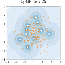
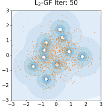
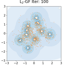
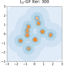
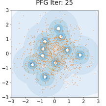
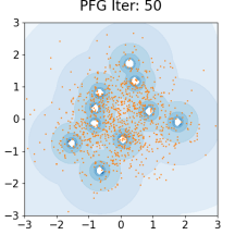
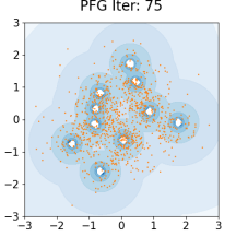
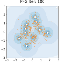
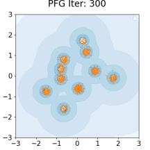
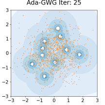
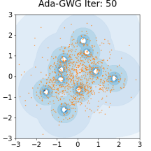
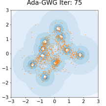
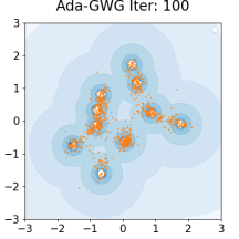
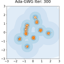
Figure 1: Comparison of sampled particles at different numbers of iterations. Upper: $\displaystyle L_{2}$-GF. Middle: PFG. Lower: Ada-GWG with $\displaystyle p_{0}=2$.

6.2 Monomial Gamma

To illustrate the effectiveness and efficiency of the adaptive method compared to the non-adaptive counterparts, we consider the heavy tailed Monomial Gamma distribution where the target $\displaystyle\pi\propto\exp(-0.3(|x_{1}|^{0.9}+|x_{2}|^{0.9}))$.

We test GWG and Ada-GWG with different choices of the initial values of $\displaystyle p$. The number of particles is $\displaystyle 1000$. Figure 3 demonstrates the KL divergence of different methods against the number of iterations. The dotted line represents GWG with fixed $\displaystyle p$, while the solid line represents the corresponding Ada-GWG that starts from the same $\displaystyle p$ at initialization.

We see that the adaptive method outperforms the non-adaptive counterpart consistently. Moreover, Ada-GWG can automatically learn the appropriate value of $\displaystyle p$ especially when the initial values of $\displaystyle p$ is set inappropriately. For example, in our case, a relatively small value of $\displaystyle p=1.5$ would be inappropriate (the dotted green line) for GWG, while Ada-GWG with the same initial value of $\displaystyle p=1.5$ is able to provide much better approximation by automatically adjusting $\displaystyle p$ during runtime. Consequently, Ada-GWG can exhibit greater robustness when determining the initial value of $\displaystyle p$.

6.3 Conditioned Diffusion

The conditioned diffusion example is a high-dimensional model arising from a Langevin SDE, with state $\displaystyle u:[0,1]\longrightarrow\mathbb{R}$ and dynamics given by

$$du_{t}=\frac{10u(1-u^{2})}{1+u^{2}}dt+dx_{t},\quad u_{0}=0,$$ (23)

where $\displaystyle x=(x_{t})_{t\geq 0}$ is a standard Brownian motion.

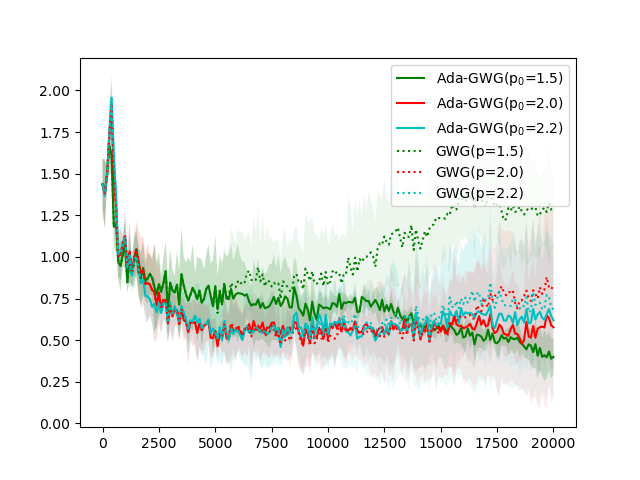
Figure 2: KL divergence of different methods. Solid line: Ada-GWG. Dotted line: GWG counterpart.

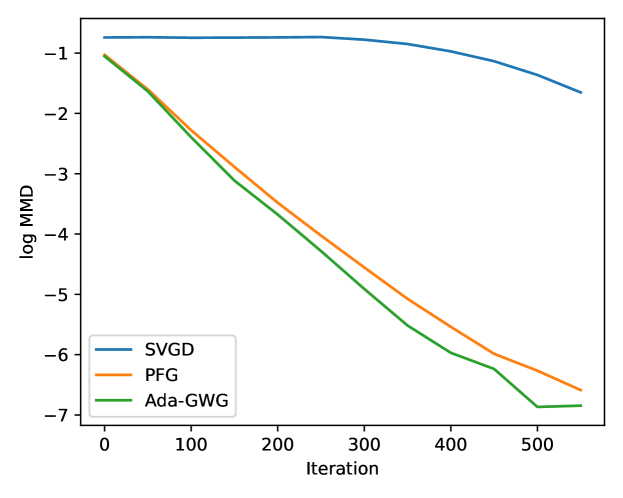
Figure 3: Comparison among PFG, Ada-GWG, SVGD in conditioned diffusion example.

This system is commonly used in molecular dynamics to represent the motion of a particle with negligible mass trapped in an energy potential with thermal fluctuations represented by the Brownian forcing [14, 12]. Given the perturbed observations $\displaystyle y$, the goal is to infer the posterior of the driving process $\displaystyle p(x|y)$. The forward operator is defined by $\displaystyle\mathcal{F}(x)=(u_{t_{1}},\cdots,u_{t_{20}})\in\mathbb{R}^{20}$, where $\displaystyle t_{i}=0.05i$. This is achieved by discretizing the above SDE (23) using an Euler-Maruyama scheme with step size $\displaystyle\Delta t=0.01$; therefore the dimensionality of the problem is $\displaystyle 100$. The noisy observations are obtained as $\displaystyle y=\mathcal{F}(x_{\text{true}})+\xi\in\mathbb{R}^{20}$, where $\displaystyle x_{\text{true}}$ is a Brownian motion path and $\displaystyle\xi\sim\mathcal{N}(0,\sigma^{2}I)$ with $\displaystyle\sigma=0.1$. The prior is given by the Brownian motion $\displaystyle x=(x_{t})_{t\geq 0}$.

We test three algorithms: PFG, Ada-GWG, and SVGD, with $\displaystyle n=1000$ particles. To obtain the ground truth posterior, we run LMC with $\displaystyle 1000$ particles in parallel, using a small step size $\displaystyle h=10^{-4}$ for $\displaystyle 10000$ iterations. Figure 3 reports the logarithmic Maximum Mean Discrepancy (MMD) curves against iterations. We observe that Ada-GWG provides best performance compared to the other methods.

6.4 Bayesian Neural Networks

We compare our algorithm with SGLD and SVGD variants on Bayesian neural networks (BNN). Following Liu & Wang [31], we conduct the two-layer network with 50 hidden units and ReLU activation function, and we use a $\displaystyle\mathrm{Gamma}(1,0.1)$ prior for the inverse covariances. The datasets are all randomly partitioned into 90% for training and 10% for testing. The mini-batch size is 100 except for Concrete on which we use 400. The particle size is 100 and the results are averaged over 10 random trials. Table 1 shows the average test RMSE and NLL and their standard deviation. We see that Ada-GWG can achieve comparable or better results than the other methods. And the adaptive method consistently improves over $\displaystyle L_{2}$-GF. Figure 4 shows the test RMSE against iterations of different methods on the Boston dataset. We can see that for this specific task, setting $\displaystyle p=3$ produces better results than when $\displaystyle p=2$. Although $\displaystyle L_{2}$-GF (i.e., GWG with $\displaystyle p=2$) is sub-optimal, our adaptive method (i.e., Ada-GWG with $\displaystyle p_{0}=2$) makes significant improvements and demonstrates comparable performance to the optimal choice of $\displaystyle p=3$. This suggests that our adaptive method is robust even if the initial exponent choice is not ideal. More comparisons of convergence results and hyperparameter tuning details can be found in the appendix.

Table 1: Averaged test RMSE and test negative log-likelihood of Bayesian Neural Networks on several UCI datasets. The results are averaged from 10 independent runs.

	Avg. Test RMSE				Avg. Test NLL
Dataset	SGLD	SVGD	$\displaystyle L_{2}$-GF	Ada-GWG	SGLD	SVGD	$\displaystyle L_{2}$-GF	Ada-GWG
Boston	$\displaystyle 3.011_{\pm 0.15}$	$\displaystyle 2.774_{\pm 0.08}$	$\displaystyle 3.072_{\pm 0.10}$	$\displaystyle\bm{2.721}_{\pm 0.08}$	$\displaystyle 2.496_{\pm 0.03}$	$\displaystyle 2.444_{\pm 0.02}$	$\displaystyle 2.547_{\pm 0.14}$	$\displaystyle\bm{2.434}_{\pm 0.02}$
Concrete	$\displaystyle 5.583_{\pm 0.25}$	$\displaystyle 4.436_{\pm 0.08}$	$\displaystyle 4.343_{\pm 0.11}$	$\displaystyle\bm{3.871}_{\pm 0.10}$	$\displaystyle 3.184_{\pm 0.04}$	$\displaystyle 3.035_{\pm 0.02}$	$\displaystyle 3.053_{\pm 0.03}$	$\displaystyle\bm{2.826}_{\pm 0.02}$
Power	$\displaystyle 4.089_{\pm 0.11}$	$\displaystyle 3.972_{\pm 0.02}$	$\displaystyle 4.014_{\pm 0.02}$	$\displaystyle\bm{3.944}_{\pm 0.01}$	$\displaystyle 2.840_{\pm 0.02}$	$\displaystyle 2.809_{\pm 0.01}$	$\displaystyle 2.824_{\pm 0.01}$	$\displaystyle\bm{2.802}_{\pm 0.01}$
Winewhite	$\displaystyle 0.677_{\pm 0.01}$	$\displaystyle 0.664_{\pm 0.01}$	$\displaystyle 0.666_{\pm 0.01}$	$\displaystyle\bm{0.660}_{\pm 0.01}$	$\displaystyle 1.033_{\pm 0.01}$	$\displaystyle 1.014_{\pm 0.01}$	$\displaystyle 1.015_{\pm 0.01}$	$\displaystyle\bm{1.006}_{\pm 0.01}$
Winered	$\displaystyle 0.600_{\pm 0.01}$	$\displaystyle 0.579_{\pm 0.01}$	$\displaystyle 0.581_{\pm 0.01}$	$\displaystyle\bm{0.575}_{\pm 0.01}$	$\displaystyle 0.910_{\pm 0.01}$	$\displaystyle 0.887_{\pm 0.02}$	$\displaystyle 0.860_{\pm 0.02}$	$\displaystyle\bm{0.839}_{\pm 0.02}$
protein	$\displaystyle\bm{4.560}_{\pm 0.04}$	$\displaystyle 4.779_{\pm 0.03}$	$\displaystyle 4.867_{\pm 0.01}$	$\displaystyle 4.686_{\pm 0.02}$	$\displaystyle\bm{2.934}_{\pm 0.01}$	$\displaystyle 2.984_{\pm 0.01}$	$\displaystyle 3.003_{\pm 0.00}$	$\displaystyle 2.964_{\pm 0.00}$

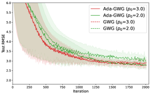
Figure 4: Test RMSE for the Bayesian Neural Networks on Boston dataset. The number in parentheses specifies the initial exponent $\displaystyle p_{0}$. The results are averaged from 10 independent runs.

7 Conclusion

We introduced a new ParVI method, called GWG, which corresponds to a generalized Wasserstein gradient flow of KL divergence. We show that our method has strong convergence guarantees in discrete time setting. We also propose an adaptive version, called Ada-GWG, that can automatically adjust the Wassertein metric to accelerate convergence. Extensive numerical results showed that Ada-GWG outperforms conventional ParVI methods.

Appendix A Minimizing Movement Scheme

A.1 Geometric Interpretation

In fact, under some mild conditions of $\displaystyle g$, the transportation cost $\displaystyle W_{c_{h}}(\cdot,\cdot)$ can induce a Wasserstein metric and thus $\displaystyle\mathcal{P}_{c_{h}}(\mathbb{R}^{d}):=\{\mu\in\mathcal{P}(\mathbb{R}^{d}):\mathbb{E}_{\mu}[g(\frac{2x}{h})]<\infty\}$ is indeed a Wasserstein space.

Proposition 1.

Let $\displaystyle g(\cdot)=g_{0}(\|\cdot\|)$ where $\displaystyle g_{0}:\mathbb{R}^{+}\cup{\{0\}}\rightarrow\mathbb{R}^{+}\cup{\{0\}}$ satisfies $\displaystyle g_{0}(0)=0$ and $\displaystyle\|\cdot\|$ can be any norm in $\displaystyle\mathbb{R}^{d}$. Then $\displaystyle g_{0}^{-1}(W_{c_{h}}(\cdot,\cdot))$ is a metric on $\displaystyle\mathcal{P}_{c_{h}}(\mathbb{R}^{d})$ if $\displaystyle g_{0}$ satisfies: (1) $\displaystyle g_{0}$ is continuous and strictly increasing; (2) $\displaystyle g_{0}$ is convex; (3) $\displaystyle\log g_{0}(x)$ is a convex function of $\displaystyle\log x$.

Proof.

Suppose $\displaystyle\pi,\mu,\nu\in\mathcal{P}_{c_{h}}$. It is obvious that $\displaystyle g_{0}^{-1}(W_{c_{h}}(\mu,\nu))=0$ if and only if $\displaystyle\mu=\nu$. Besides, $\displaystyle g_{0}^{-1}(W_{c_{h}}(\cdot,\cdot))$ is symmetric. In the rest part of proof we aim to show that $\displaystyle g_{0}^{-1}(W_{c_{h}}(\mu,\pi))+g_{0}^{-1}(W_{c_{h}}(\nu,\pi))\geq g_{0}^{-1}(W_{c_{h}}(\mu,\nu))$. By Gluing lemma [40], we can construct random variables $\displaystyle X\sim\pi,Y\sim\mu,Z\sim\nu$ such that $\displaystyle(X,Y)$, $\displaystyle(X,Z)$ are the optimal coupling of $\displaystyle(\pi,\mu)$ and $\displaystyle(\pi,\nu)$ for transportation cost $\displaystyle W_{c_{h}}$, respectively. Then we have

$$g_{0}^{-1}(W_{c_{h}}(\mu,\nu)) \leq g_{0}^{-1}\left(\mathbb{E}g_{0}\left(\frac{\|Y-Z\|}{h}\right)\right)$$

$$\leq g_{0}^{-1}\left(\mathbb{E}g_{0}\left(\frac{\|X-Y\|+\|X-Z\|}{h}\right)\right)$$

$$\leq g_{0}^{-1}\left(\mathbb{E}g_{0}\left(\frac{\|X-Y\|}{h}\right)\right)+g_{0}^{-1}\left(\mathbb{E}g_{0}\left(\frac{\|X-Z\|}{h}\right)\right)$$

$$=g_{0}^{-1}(W_{c_{h}}(\mu,\pi))+g_{0}^{-1}(W_{c_{h}}(\pi,\nu)).$$

Here the last inequality is due to generalized Minkowski’s inequality [33]. ∎

The conditions in Proposition 1 are mild and the most common choices of Young function $\displaystyle g$ satisfy them, and hence can induce a Wasserstein space the generalized Wasserstein gradient flow. Some typical examples of $\displaystyle g_{0}$ include $\displaystyle|x|^{p},\exp(ax^{2})-1,x\exp(ax^{b})$, while the norm $\displaystyle\|\cdot\|$ in $\displaystyle\mathbb{R}^{d}$ can be $\displaystyle\|\cdot\|_{p},\|\cdot\|_{H}$ and so on.

A.2 Derivation of Generalized Wasserstein Gradient Flow

Theorem 2 (Restatement of Theorem 1).

Given a continuously differentiable Young function $\displaystyle g$ and step size $\displaystyle h>0$, define cost function $\displaystyle c_{h}(x,y)=g(\frac{x-y}{h})h$. Suppose that $\displaystyle\pi,\mu_{kh}\in\mathcal{P}_{c_{h}}(\mathbb{R}^{d}):=\{\mu\in\mathcal{P}(\mathbb{R}^{d}):\mathbb{E}_{\mu}[g(\frac{2x}{h})]<\infty\}$. If $\displaystyle g$ satisfies assumptions in Proposition 1, $\displaystyle\mathcal{P}_{c_{h}}(\mathbb{R}^{d})$ is a Wasserstein space equipped with Wasserstein metric. Consider MMS under transportation cost $\displaystyle W_{c_{h}}$:

$$\mu_{(k+1)h}:=\operatorname*{arg\,min}_{\mu\in\mathcal{P}_{c_{h}}(\mathbb{R}^{d})}D_{\mathrm{KL}}(\mu\|\pi)+W_{c_{h}}(\mu,\mu_{kh}).$$ (24)

Denote the optimal transportation map under $\displaystyle W_{c_{h}}$ from $\displaystyle\mu_{(k+1)h}$ to $\displaystyle\mu_{kh}$ by $\displaystyle T_{k}(\cdot)$. Then we have

$$\frac{T_{k}(x)-x}{h}=-\nabla g^{*}\left(\nabla\log\pi(x)-\nabla\log\mu_{(k+1)h}(x)\right).$$ (25)

Proof.

By Kantorovich duality [39], the optimal transportation cost (3) has an equivalent definition:

$$W_{c}(\mu,\nu)=\sup_{\varphi}\int\varphi d\mu+\int\varphi^{c}d\nu,\ \text{where}\ \varphi^{c}(y):=\inf_{x\in\mathbb{R}^{d}}c(x,y)-\varphi(x).$$ (26)

Take the functional derivative of the optimization problem (24) and define the optimal $\displaystyle\varphi$ in (26) as $\displaystyle\psi$. The following holds:

$$\frac{\delta}{\delta\mu}D_{\mathrm{KL}}(\mu_{(k+1)h}\|\pi)+\psi_{kh}=\text{const}.$$ (27)

Here the reason for have a constant instead of zero is that we constrain $\displaystyle\mu_{(k+1)h}$ in the space of smooth probability density. Note that $\displaystyle c_{h}(x,y)\leq\frac{1}{2}\left(g(\frac{2x}{h})+g(\frac{2y}{h})\right)$ and $\displaystyle\mu_{kh},\mu_{(k+1)h}\in\mathcal{P}_{c_{h}}(\mathbb{R}^{d})$, then by the fundamental theorem of optimal transportation [39],

$$\psi_{kh}(x)+\psi_{kh}^{c_{h}}(y)=c_{h}(x,y),\ \text{for}\ y=T_{k}(x),$$ (28)

which implies $\displaystyle\nabla\psi_{kh}(x)=\nabla_{x}c_{h}(x,y)=\nabla g(\frac{x-y}{h})$, i.e.,

$$x-y=\nabla g^{*}(\nabla\psi_{kh}(x))h.$$ (29)

Combine this equation with (27) and thus the optimal map is given by

$$\frac{T_{k}(x)-x}{h} =-\nabla g^{*}(-\nabla\frac{\delta}{\delta\mu}D_{\mathrm{KL}}(\mu_{(k+1)h}\|\pi))$$

$$=-\nabla g^{*}(\nabla\log\frac{\pi}{\mu_{(k+1)h}}).$$

∎

Appendix B Details of Motivating Example

We use Example 1 to illustrate the benefits of choosing general Young function $\displaystyle g^{*}$, which is also discussed in [4, 46].

We follow the procedures of [46]. For convenience, let $\displaystyle\pi_{0}=\mathcal{N}(-m,1),\pi_{1}=\mathcal{N}(m,1)$ and rewrite $\displaystyle\pi=\frac{1}{2}\pi_{0}+\frac{1}{2}\pi_{1},\mu=\frac{3}{4}\pi_{0}+\frac{1}{4}\pi_{1}$. The lower bound of KL divergence follows from [15] and Pinsker inequality. In addition, [4] shows

$$\nabla\log\pi-\nabla\log\mu=-m\frac{\pi_{0}\pi_{1}}{2\pi\mu}.$$ (30)

Also note that $\displaystyle\frac{\pi_{0}}{\pi_{1}}=\exp(-2mx)$. Therefore for any $\displaystyle q\geq 1$, the following bound holds:

$$\mathbb{E}_{\mu}\bigg{|}\bigg{|}\nabla\log\frac{\pi}{\mu}\bigg{|}\bigg{|}_{q}^{q} =\frac{m^{q}}{2^{q}}\int\frac{\pi_{0}^{q}\pi_{1}^{q}}{\mu^{q-1}\pi^{q}}dx$$ (31)

$$=4^{q-1}m^{q}\int\frac{\pi_{0}^{q}\pi_{1}^{q}}{(3\pi_{0}+\pi_{1})^{q-1}(\pi_{0}+\pi_{1})^{q}}dx$$

$$\geq 4^{q-1}m^{q}\left(\int_{x\geq\frac{1}{m}}\frac{\pi_{0}^{q}}{(1+e^{-2})^{q}\pi_{1}^{q-1}(1+3e^{-2})^{q-1}}dx+\int_{x\leq-\frac{1}{m}}\frac{\pi_{1}^{q}}{(1+e^{-2})^{q}\pi_{0}^{q-1}(3+e^{-2})^{q-1}}dx\right).$$

$$\int_{x\geq\frac{1}{m}}\frac{\pi_{0}^{q}}{\pi_{1}^{q-1}}dx =\int_{x\geq\frac{1}{m}}\frac{1}{\sqrt{2\pi}}\exp(-\frac{1}{2}(x+m)^{2}-2m(q-1)x)dx$$ (32)

$$=\mathbf{Prob}_{\mathcal{N}(0,1)}\{Z\geq(2q-1)m+\frac{1}{m}\}\exp(2q(q-1)m^{2})$$

$$\geq\frac{3}{4}\frac{1}{(2q-1)m+\frac{1}{m}}\frac{1}{\sqrt{2\pi}}\exp\left(-\frac{1}{2}((2q-1)m+\frac{1}{m})^{2}+2q(q-1)m^{2}\right)$$

$$\geq\frac{3}{4}\frac{1}{2qm}\frac{1}{\sqrt{2\pi}}\exp(-\frac{1}{2}m^{2}-2q+\frac{1}{2}).$$

Here the first inequality is by $\displaystyle\mathbf{Prob}_{\mathcal{N}(0,1)}\{Z\geq t\}\geq(\frac{1}{t}-\frac{1}{t^{3}})\frac{1}{\sqrt{2\pi}}\exp(-\frac{t^{2}}{2})$ for any $\displaystyle t>0$ and $\displaystyle(2q-1)m+\frac{1}{m}\geq 2$. Similarly, we can prove that

$$\int_{x\leq-\frac{1}{m}}\frac{\pi_{1}^{q}}{\pi_{0}^{q-1}}dx\geq\frac{3}{4}\frac{1}{2qm}\frac{1}{\sqrt{2\pi}}\exp(-\frac{1}{2}m^{2}-2q+\frac{1}{2}).$$ (33)

Plug (32) and (33) in (31),

$$\mathbb{E}_{\mu}\bigg{|}\bigg{|}\nabla\log\frac{\pi}{\mu}\bigg{|}\bigg{|}_{q}^{q} \geq\frac{1}{q}m^{q-1}\exp(-\frac{m^{2}}{2})\cdot\frac{3}{4^{3}}\sqrt{\frac{2e}{\pi}}4^{q}(e^{2}+1)^{-q}\left[(\frac{1}{1+3e^{-2}})^{q-1}+(\frac{1}{3+e^{-2}})^{q-1}\right]$$

$$\geq\frac{1}{q}m^{q-1}\exp(-\frac{m^{2}}{2})\cdot\frac{3}{4^{3}}\sqrt{\frac{2e}{\pi}}(1+3e^{-2})\left[\frac{4}{(1+e^{2})(1+3e^{-2})}\right]^{q}$$

$$\geq\frac{0.08}{qm}(\frac{m}{3})^{q}\exp(-\frac{m^{2}}{2}).$$

As for the upper bound,

$$\mathbb{E}_{\mu}\bigg{|}\bigg{|}\nabla\log\frac{\pi}{\mu}\bigg{|}\bigg{|}_{q}^{q} =\frac{m^{q}}{2^{q}}\int\frac{\pi_{0}^{q}\pi_{1}^{q}}{\mu^{q-1}\pi^{q}}dx$$ (34)

$$=4^{q-1}m^{q}\int\frac{\pi_{0}^{q}\pi_{1}^{q}}{(3\pi_{0}+\pi_{1})^{q-1}(\pi_{0}+\pi_{1})^{q}}dx$$

$$\leq 4^{q-1}m^{q}\left(\int_{x\geq 0}\frac{\pi_{0}^{q}}{\pi_{1}^{q-1}}dx+\int_{x\leq 0}\frac{\pi_{1}^{q}}{\pi_{0}^{q-1}}dx\right).$$

$$\int_{x\geq 0}\frac{\pi_{0}^{q}}{\pi_{1}^{q-1}}dx =\int_{x\geq 0}\frac{1}{\sqrt{2\pi}}\exp(-\frac{1}{2}(x+m)^{2}-2m(q-1)x)dx$$ (35)

$$=\mathbf{Prob}_{\mathcal{N}(0,1)}\{Z\geq(2q-1)m\}\exp(2q(q-1)m^{2})$$

$$\leq\frac{1}{(2q-1)m}\frac{1}{\sqrt{2\pi}}\exp\left(-\frac{1}{2}((2q-1)m)^{2}+2q(q-1)m^{2}\right)$$

$$\leq\frac{1}{qm}\frac{1}{\sqrt{2\pi}}\exp(-\frac{1}{2}m^{2}).$$

Here the first inequality is by $\displaystyle\mathbf{Prob}_{\mathcal{N}(0,1)}\{Z\geq t\}\leq\frac{1}{t}\frac{1}{\sqrt{2\pi}}\exp(-\frac{t^{2}}{2})$ for any $\displaystyle t>0$. Similarly, we can prove that

$$\int_{x\leq 0}\frac{\pi_{1}^{q}}{\pi_{0}^{q-1}}dx\leq\frac{1}{qm}\frac{1}{\sqrt{2\pi}}\exp(-\frac{1}{2}m^{2}).$$ (36)

Therefore

$$\mathbb{E}_{\mu}\bigg{|}\bigg{|}\nabla\log\frac{\pi}{\mu}\bigg{|}\bigg{|}_{q}^{q} \leq 4^{q-1}m^{q}\cdot\frac{2}{qm}\frac{1}{\sqrt{2\pi}}\exp(-\frac{1}{2}m^{2})$$

$$\leq\frac{0.2}{qm}(4m)^{q}\exp(-\frac{m^{2}}{2}).$$

Appendix C Asymptotic Normality of Estimator

In practice, there are finite particles and we can only get a Monte Carlo estimation of (13). But our theoretical analysis is based on the population loss. With this concern, we show that the maximum point of estimation (14) have good statistical properties. To be specific, the estimator converges to true maximum point with asymptotic normality under mild conditions. Similar properties are also studied in [5, 37, 27].

Define objective function $\displaystyle\ell(w,x):=\nabla\log{\pi(x)}^{T}f_{w}(x)+\nabla_{x}\cdot f_{w}(x)-g(f_{w}(x))$.

Assumption 4.

$\displaystyle\mathcal{W}$ is compact and $\displaystyle\mathcal{L}(\cdot)$ defined in (13) has a unique maximum point $\displaystyle w^{*}\in\text{int}(\mathcal{W})$.

Assumption 5.

$\displaystyle f_{w}(x),\nabla_{x}f_{w}(x)$ are continuous with $\displaystyle w$. $\displaystyle\max\left\{\|f_{w}(x)\|,|\nabla_{x}\cdot f_{w}(x)|,g(f_{w}(x))\right\}\leq M_{0}(x)$ for some $\displaystyle M_{0}\in\mathcal{L}^{1}(\mu)$.

Assumption 6.

There exists a neighborhood $\displaystyle\mathcal{N}$ of $\displaystyle w^{*}$ such that $\displaystyle\ell(\cdot,x)$ is twice differentiable in $\displaystyle\mathcal{N}$ and $\displaystyle\|\nabla^{2}\ell(w,x)\|\leq M_{1}(x)$ for all $\displaystyle w\in\mathcal{N}$. Additionally, assume $\displaystyle M_{1}\in\mathcal{L}^{1}(\mu)$ and $\displaystyle H:=\nabla^{2}\mathcal{L}(w^{*})$ is non-singular.

Theorem 1.

Given $\displaystyle x_{1},\cdots,x_{n}\overset{{\it i.i.d.}}{\sim}\mu$, let $\displaystyle\widehat{w}_{n}:=\operatorname*{arg\,min}_{w}\widehat{\mathcal{L}}_{n}(w):=\frac{1}{n}\sum_{i=1}^{n}\ell(w,x_{i})$. Under Assumption 4-6, we have

$$\sqrt{n}(\widehat{w}_{n}-w^{*})\overset{p}{\to}\mathcal{N}\left(0,H^{-1}\Sigma H^{-1}\right),$$ (37)

where $\displaystyle\Sigma=\mathbb{E}_{\mu}\nabla_{w}\ell(w^{*},\cdot)\otimes\nabla_{w}\ell(w^{*},\cdot)$.

Proof.

Note that under Assumption 5, $\displaystyle|\ell(w,x)|\leq M(x)$ for some $\displaystyle M\in\mathcal{L}^{1}(\mu)$. By Newey & McFadden [35, Lemma 2.4, Theorem 2.1], $\displaystyle\widehat{w}_{n}$ is weakly consistent for $\displaystyle w^{*}$. Additionally, since $\displaystyle w^{*}$ is the maximum point of $\displaystyle\mathcal{L}$ and by Central Limit Theorem,

$$\sqrt{n}\nabla\widehat{\mathcal{L}}_{n}(w^{*})=\frac{1}{\sqrt{n}}\sum_{i=1}^{n}\nabla_{w}\ell(w^{*},x_{i})\overset{p}{\to}\mathcal{N}(0,\Sigma).$$

By Assumption 6 and Newey & McFadden [35, Lemma 2.4], the second order derivative converges uniformly, i.e.

$$\sup_{w\in\mathcal{N}}\|\nabla^{2}\widehat{\mathcal{L}}_{n}(w)-\nabla^{2}\mathcal{L}(w)\|\overset{p}{\to}0.$$

Finally, the result follows Newey & McFadden [35, Theorem 3.1].

∎

Appendix D Proof in Section 4

We first justify our Assumption 1 and 2, then present some crucial lemmas and finish the proof of convergence results. Our proof procedure uses interpolation process of discrete dynamics, following [38, 4]. Informally, the difference between discrete dynamics and continuous dynamics consists of two parts: discretization error and estimation error (by neural nets). We bound the discretization error in Lemma 3, 4 and the estimation error in Lemma 5, 6.

D.1 Justification for Assumption 1 and 2

Proof of Proposition 1.

It suffices to show that there exists $\displaystyle\varepsilon_{2}<\infty$ such that for any $\displaystyle a,b\in\mathbb{R}$, the following inequality holds:

$$|b-\text{sgn}(a)|a|^{q-1}|^{p}\leq\varepsilon_{1}\frac{|a|^{q}}{q}+\varepsilon_{2}\left(\frac{|a|^{q}}{q}-ab+\frac{|b|^{p}}{p}\right).$$ (38)

If $\displaystyle a=0$, then $\displaystyle\varepsilon_{2}\geq p$ is sufficient. Without loss of generality, suppose $\displaystyle a=1$ (by replacing $\displaystyle b$ with $\displaystyle\text{sgn}(a)b/|a|^{q-1}$). We only need to show that

$$|b-1|^{p}\leq\varepsilon_{1}+\varepsilon_{2}\left(\frac{1}{q}-b+\frac{|b|^{p}}{p}\right).$$ (39)

(1) Case $\displaystyle p\geq 2$.

Let $\displaystyle\varepsilon_{1}=0$. Since $\displaystyle\lim_{b\to 1}\frac{|b-1|^{p}}{\frac{1}{q}-b+\frac{|b|^{p}}{p}}=\lim_{b\to 1}\frac{2|b-1|^{p-2}}{p-1}\leq 2$, so there exists $\displaystyle\delta>0$ such that when $\displaystyle b\in[1-\delta,1+\delta]$, (39) holds if $\displaystyle\varepsilon_{2}\geq p+1>2$. Also note that $\displaystyle f(b)=\frac{|b-1|^{p}}{\frac{1}{q}-b+\frac{|b|^{p}}{p}}$ is a continuous function on $\displaystyle\mathbb{R}\backslash(1-\delta,1+\delta)$ and $\displaystyle\lim_{b\to\infty}f(b)=p<+\infty$. Therefore, $\displaystyle f(b)$ is bounded on $\displaystyle\mathbb{R}\backslash[1-\delta,1+\delta]$ and thus (39) holds for finite $\displaystyle\varepsilon_{2}$. It’s obvious that $\displaystyle\varepsilon_{2}$ only depends on $\displaystyle p$ in this case.

(2) Case $\displaystyle p<2$.

Similarly, let $\displaystyle\delta=\varepsilon_{1}^{1/p}$. When $\displaystyle b\in[1-\delta,1+\delta]$, (39) will trivially hold for any $\displaystyle\varepsilon_{2}>0$. Also, $\displaystyle f(b)$ is bounded on $\displaystyle\mathbb{R}\backslash[1-\delta,1+\delta]$ and thus there exists finite $\displaystyle\varepsilon_{2}$ determined by $\displaystyle p,\delta$ such that (39) holds. ∎

D.2 Main Lemmas

Lemma 1.

For any $\displaystyle t\in(kh,(k+1)h)$, $\displaystyle\partial_{t}D_{\mathrm{KL}}(\mu_{t}\|\pi)=-\mathbb{E}_{\mu_{t}}\left\langle\nabla\log{\frac{\pi}{\mu_{t}}},\mathbb{E}[v_{k}(X_{kh})|X_{t}=\cdot]\right\rangle$

Proof.

Let $\displaystyle\mu_{t|\mathcal{F}_{kh}}$ denote the law of $\displaystyle X_{t}$ conditioned on the filtration $\displaystyle\mathcal{F}_{kh}$ at time $\displaystyle kh$. Then by Fokker-Planck equation, we have

$$\partial_{t}\mu_{t|\mathcal{F}_{kh}}=-\text{div}\left(\mu_{t|\mathcal{F}_{kh}}v_{k}(X_{kh})\right).$$

Then we take expectation of the above equation; by Bayesian formula [38],

$$\partial_{t}\mu_{t} =-\text{div}\ \mathbb{E}[\mu_{t|\mathcal{F}_{kh}}v_{k}(X_{kh})]$$

$$=-\text{div}\left(\mu_{t}\mathbb{E}[v_{k}(X_{kh})|X_{t}=\cdot]\right)$$

Hence

$$\partial_{t}D_{\mathrm{KL}}(\mu_{t}\|\pi)=-\mathbb{E}_{\mu_{t}}\left\langle\nabla\log{\frac{\pi}{\mu_{t}}},\mathbb{E}[v_{k}(X_{kh})|X_{t}=\cdot]\right\rangle.$$

∎

Lemma 2.

Suppose that $\displaystyle h<\frac{1}{G_{2}}$. Under Assumption 3, for any $\displaystyle t\in[kh,(k+1)h],\ q>1,\frac{1}{p}+\frac{1}{q}=1$,

$$\mathbb{E}_{\mu_{t}}\bigg{|}\bigg{|}\nabla\log{\frac{\mu_{t}}{\mu_{kh}}}\bigg{|}\bigg{|}_{q}^{q}\leq\left(M_{p}(1-hG_{2})^{-1}dh\right)^{q}$$

Proof.

Note that $\displaystyle\log\frac{\mu_{t}}{\mu_{kh}}=-\log\det\left(I_{d}+(t-kh)\nabla v_{k}\right)$ since $\displaystyle x\mapsto x+(t-kh)v_{k}(x)$ is an orientation-preserving diffeomorphism under $\displaystyle h<\frac{1}{G_{2}}$. Then the following holds:

$$\bigg{|}\bigg{|}\nabla\log\frac{\mu_{t}}{\mu_{kh}}(x)\bigg{|}\bigg{|}_{q} =\sup_{\|z\|_{p}=1}\left\langle\nabla\log\frac{\mu_{t}}{\mu_{kh}}(x),z\right\rangle$$

$$=\sup_{\|z\|_{p}=1}\lim_{\delta\to 0}\bigg{|}\log\det\left(I_{d}+(t-kh)\nabla v_{k}(x+\delta z)\right)-\log\det\left(I_{d}+(t-kh)\nabla v_{k}(x)\right)\bigg{|}$$

$$\leq\sup_{\|z\|_{p}=1}\lim_{\delta\to 0}(t-kh)\|\nabla v_{k}(x+\delta z)-\nabla v_{k}(x)\|_{2}(1-hG_{2})^{-1}d$$

$$\leq M_{p}(1-hG_{2})^{-1}dh.$$

Here the first equation is due to Young’s inequality and the second equation follows the definition of gradient. The inequality in the third line is due to Lemma 13 and the last one is by Assumption 3. With this uniform bound we finish the proof. ∎

Lemma 3.

Under Assumption 1, 3, and the same conditions in Lemma 2,

$$\mathbb{E}_{\mu_{t}}\bigg{|}\bigg{|}\nabla g^{*}(\nabla\log\frac{\pi}{\mu_{t}})-\nabla g^{*}(\nabla\log\frac{\pi}{\mu_{kh}})\bigg{|}\bigg{|}_{p}^{p}\leq c_{1}\mathbb{E}_{\mu_{t}}\bigg{|}\bigg{|}\nabla\log\frac{\pi}{\mu_{t}}\bigg{|}\bigg{|}_{q}^{q}+c_{2}\left(M_{p}(1-hG_{2})^{-1}dh\right)^{q}$$

where $\displaystyle c_{1},c_{2}$ are defined as:

$$(c_{1},c_{2})=\left\{\begin{array}[]{ll}(0,\ 2^{p-q})&\text{if}\ q\leq 2,\\ \left(3^{-p},\ \min\left\{3^{q-p}(\frac{p}{q})^{\frac{q-p}{q-1}}(1-\frac{p}{q})^{\frac{q-p}{p}},(q-1)^{p}\left(\frac{(\frac{4}{3})^{\frac{1}{q-1}}}{(\frac{4}{3})^{\frac{1}{q-1}}-1}\right)^{q-p}\right\}\right)&\text{otherwise}.\end{array}\right.$$ (40)

Proof.

Since $\displaystyle g^{*}(x)=\frac{1}{q}\|x\|_{q}^{q}$, we have $\displaystyle\nabla g^{*}(x)=\text{sgn}(x)\odot|x|^{q-1}$. Here $\displaystyle\odot$ means entry-wise product. Apply Lemma 14 entry-wise and thus

$$\mathbb{E}_{\mu_{t}}\bigg{|}\bigg{|}\nabla g^{*}(\nabla\log\frac{\pi}{\mu_{t}})-\nabla g^{*}(\nabla\log\frac{\pi}{\mu_{kh}})\bigg{|}\bigg{|}_{p}^{p} \leq c_{1}\mathbb{E}_{\mu_{t}}\bigg{|}\bigg{|}\nabla\log\frac{\pi}{\mu_{t}}\bigg{|}\bigg{|}_{q}^{q}+c_{2}\mathbb{E}_{\mu_{t}}\bigg{|}\bigg{|}\nabla\log\frac{\mu_{t}}{\mu_{kh}}\bigg{|}\bigg{|}_{q}^{q}$$

$$\leq c_{1}\mathbb{E}_{\mu_{t}}\bigg{|}\bigg{|}\nabla\log\frac{\pi}{\mu_{t}}\bigg{|}\bigg{|}_{q}^{q}+c_{2}\left(M_{p}(1-hG_{2})^{-1}dh\right)^{q}.$$

The second inequality is due to Lemma 2. ∎

Lemma 4.

Under Assumption 2, 3 and the same conditions in Lemma 2,

$$\mathbb{E}_{\mu_{t}}\bigg{|}\bigg{|}\nabla g^{*}(\nabla\log\frac{\pi}{\mu_{t}})-\nabla g^{*}(\nabla\log\frac{\pi}{\mu_{kh}})\bigg{|}\bigg{|}_{2}^{2}\leq\beta^{2}\left(M_{2}(1-hG_{2})^{-1}dh\right)^{2}$$

Proof.

Note that $\displaystyle g^{*}$ is $\displaystyle\beta$-smooth and by Lemma 2,

$$\mathbb{E}_{\mu_{t}}\bigg{|}\bigg{|}\nabla g^{*}(\nabla\log\frac{\pi}{\mu_{t}})-\nabla g^{*}(\nabla\log\frac{\pi}{\mu_{kh}})\bigg{|}\bigg{|}_{2}^{2} \leq\beta^{2}\mathbb{E}_{\mu_{t}}\bigg{|}\bigg{|}\nabla\log\frac{\mu_{t}}{\mu_{kh}}\bigg{|}\bigg{|}_{2}^{2}$$

$$\leq\beta^{2}\left(M_{2}(1-hG_{2})^{-1}dh\right)^{2}.$$

∎

Lemma 5.

Suppose that $\displaystyle h<\min\left\{\frac{1}{4G_{p}},\frac{1}{G_{2}}\right\}$. Under Assumption 1, 3, for any $\displaystyle t\in[kh,(k+1)h]$,

$$\qquad\mathbb{E}_{\mu_{t}}\bigg{|}\bigg{|}\nabla g^{*}(\nabla\log\frac{\pi}{\mu_{kh}})-\mathbb{E}[v_{k}(X_{kh})|X_{t}=\cdot]\bigg{|}\bigg{|}_{p}^{p}$$

$$\qquad\qquad\leq\frac{2^{p-1}(1-hG_{2})^{-d}}{1-(4G_{p}h)^{p}}\varepsilon_{k}+\frac{2^{p-1}(4G_{p}h)^{p}}{1-(4G_{p}h)^{p}}\left((1+c_{1})\mathbb{E}_{\mu_{t}}\bigg{|}\bigg{|}\nabla\log\frac{\pi}{\mu_{t}}\bigg{|}\bigg{|}_{q}^{q}+c_{2}\left(M_{p}(1-hG_{2})^{-1}dh\right)^{q}\right),$$

where $\displaystyle c_{1},c_{2}$ are defined in (40).

Proof.

By Jensen’s inequality,

$$\mathbb{E}_{\mu_{t}}\bigg{|}\bigg{|}\nabla g^{*}(\nabla\log\frac{\pi}{\mu_{kh}})-\mathbb{E}[v_{k}(X_{kh})|X_{t}=\cdot]\bigg{|}\bigg{|}_{p}^{p}$$ (41)

$$\qquad\qquad\leq 2^{p-1}\left\{\mathbb{E}_{\mu_{t}}\bigg{|}\bigg{|}\nabla g^{*}(\nabla\log\frac{\pi}{\mu_{kh}})-v_{k}\bigg{|}\bigg{|}_{p}^{p}+\mathbb{E}_{\mu_{t}}\bigg{|}\bigg{|}v_{k}-\mathbb{E}[v_{k}(X_{kh})|X_{t}=\cdot]\bigg{|}\bigg{|}_{p}^{p}\right\}$$

$$\qquad\qquad\leq 2^{p-1}\left\{\mathbb{E}_{\mu_{t}}\bigg{|}\bigg{|}\nabla g^{*}(\nabla\log\frac{\pi}{\mu_{kh}})-v_{k}\bigg{|}\bigg{|}_{p}^{p}+\mathbb{E}\bigg{|}\bigg{|}v_{k}(X_{t})-v_{k}(X_{kh})\bigg{|}\bigg{|}_{p}^{p}\right\}.$$

Under Assumption 3 and Jensen’s inequality,

$$\mathbb{E}\bigg{|}\bigg{|}v_{k}(X_{t})-v_{k}(X_{kh})\bigg{|}\bigg{|}_{p}^{p}$$

$$\qquad\qquad\leq(G_{p})^{p}\ \mathbb{E}\|X_{t}-X_{kh}\|_{p}^{p}$$

$$\qquad\qquad\leq(G_{p}h)^{p}\ \mathbb{E}\bigg{|}\bigg{|}v_{k}(X_{kh})\bigg{|}\bigg{|}_{p}^{p}$$

$$\qquad\qquad\leq(G_{p}h)^{p}4^{p-1}\left\{\mathbb{E}\bigg{|}\bigg{|}v_{k}(X_{kh})-v_{k}(X_{t})\bigg{|}\bigg{|}_{p}^{p}+\mathbb{E}\bigg{|}\bigg{|}v_{k}(X_{t})-\nabla g^{*}\left(\nabla\log\frac{\pi}{\mu_{kh}}(X_{t})\right)\bigg{|}\bigg{|}_{p}^{p}\right.$$

$$\qquad\qquad\qquad\left.+\ \mathbb{E}\bigg{|}\bigg{|}\nabla g^{*}\left(\nabla\log\frac{\pi}{\mu_{kh}}(X_{t})\right)-\nabla g^{*}\left(\nabla\log\frac{\pi}{\mu_{t}}(X_{t})\right)\bigg{|}\bigg{|}_{p}^{p}+\mathbb{E}\bigg{|}\bigg{|}\nabla g^{*}\left(\nabla\log\frac{\pi}{\mu_{t}}(X_{t})\right)\bigg{|}\bigg{|}_{p}^{p}\right\}.$$

Rearrange the above inequality and thus

$$\mathbb{E}\bigg{|}\bigg{|}v_{k}(X_{t})-v_{k}(X_{kh})\bigg{|}\bigg{|}_{p}^{p}$$ (42)

$$\qquad\qquad\leq\left(1-(4G_{p}h)^{p}\right)^{-1}(4G_{p}h)^{p}\left\{\mathbb{E}_{\mu_{t}}\bigg{|}\bigg{|}v_{k}-\nabla g^{*}(\nabla\log\frac{\pi}{\mu_{kh}})\bigg{|}\bigg{|}_{p}^{p}\right.$$

$$\qquad\qquad\qquad\left.+\ \mathbb{E}_{\mu_{t}}\bigg{|}\bigg{|}\nabla g^{*}\nabla\log\frac{\pi}{\mu_{kh}})-\nabla g^{*}(\nabla\log\frac{\pi}{\mu_{t}})\bigg{|}\bigg{|}_{p}^{p}+\mathbb{E}_{\mu_{t}}\bigg{|}\bigg{|}\nabla g^{*}(\nabla\log\frac{\pi}{\mu_{t}})\bigg{|}\bigg{|}_{p}^{p}\right\}.$$

Again note that $\displaystyle\frac{\mu_{t}}{\mu_{kh}}=\det\left(I_{d}+(t-kh)\nabla v_{k}\right)^{-1}$, so

$$\sup_{x}\frac{\mu_{t}}{\mu_{kh}}(x)\leq\left(\|(I_{d}+(t-kh)\nabla v_{k}(x))^{-1}\|_{2}\right)^{d}\leq(1-hG_{2})^{-d}.$$

Then by Assumption 1,

$$\mathbb{E}_{\mu_{t}}\bigg{|}\bigg{|}v_{k}-\nabla g^{*}(\nabla\log\frac{\pi}{\mu_{kh}})\bigg{|}\bigg{|}_{p}^{p}\leq(1-hG_{2})^{-d}\mathbb{E}_{\mu_{kh}}\bigg{|}\bigg{|}v_{k}-\nabla g^{*}(\nabla\log\frac{\pi}{\mu_{kh}})\bigg{|}\bigg{|}_{p}^{p}\leq(1-hG_{2})^{-d}\varepsilon_{k}.$$ (43)

Combining Lemma 3 with (42),(43) and plugging them into (41), we finish the proof. ∎

Lemma 6.

Suppose that $\displaystyle h<\frac{1}{4G_{2}}$. Under Assumption 2, 3, for any $\displaystyle t\in[kh,(k+1)h]$,

$$\qquad\mathbb{E}_{\mu_{t}}\bigg{|}\bigg{|}\nabla g^{*}(\nabla\log\frac{\pi}{\mu_{kh}})-\mathbb{E}[v_{k}(X_{kh})|X_{t}=\cdot]\bigg{|}\bigg{|}_{2}^{2}$$

$$\qquad\qquad\leq\frac{2(1-hG_{2})^{-d}}{1-(4G_{2}h)^{2}}\varepsilon_{k}+\frac{2(4G_{2}h)^{2}\beta^{2}}{1-(4G_{2}h)^{2}}\left(\mathbb{E}_{\mu_{t}}\bigg{|}\bigg{|}\nabla\log\frac{\pi}{\mu_{t}}\bigg{|}\bigg{|}_{2}^{2}+\left(M_{2}(1-hG_{2})^{-1}dh\right)^{2}\right).$$

Proof.

The procedure is exactly the same with Lemma 5. The only difference appears when applying Lemma 4 instead of Lemma 3 in the last step. ∎

Lemma 7.

Suppose that $\displaystyle h\leq\min\left\{\frac{1}{36G_{p}},\frac{1-2^{-\frac{1}{q}}}{G_{2}}\right\}$. Under Assumption 1, 3, for any $\displaystyle t\in(kh,(k+1)h)$,

$$\partial_{t}D_{\mathrm{KL}}(\mu_{t}\|\pi)\leq-\frac{1}{12}\mathbb{E}_{\mu_{t}}\bigg{|}\bigg{|}\nabla\log\frac{\pi}{\mu_{t}}\bigg{|}\bigg{|}_{q}^{q}+A_{1}(M_{p}dh)^{q}+A_{2}(1-hG_{2})^{-d}\varepsilon_{k},$$

where $\displaystyle A_{1},A_{2}$ are constants only depending on $\displaystyle q$:

$$(A_{1},A_{2})=\left\{\begin{array}[]{ll}(\frac{2^{p+2}}{p},\ 2^{p})&\text{if}\ q\leq 2,\\ (\frac{7c_{2}}{p},\ \frac{3}{p})&\text{otherwise}.\end{array}\right.$$ (44)

Here $\displaystyle c_{2}$ is defined in (40).

Proof.

By Lemma 1 and Young’s inequality, for any $\displaystyle\lambda_{1},\lambda_{2}>0$,

$$\partial_{t}D_{\mathrm{KL}}(\mu_{t}\|\pi) =-\mathbb{E}_{\mu_{t}}\left\langle\nabla\log\frac{\pi}{\mu_{t}},\nabla g^{*}(\nabla\log\frac{\pi}{\mu_{t}})\right\rangle$$

$$\quad+\mathbb{E}_{\mu_{t}}\left\langle\nabla\log\frac{\pi}{\mu_{t}},\nabla g^{*}(\nabla\log\frac{\pi}{\mu_{t}})-\nabla g^{*}(\nabla\log\frac{\pi}{\mu_{kh}})\right\rangle$$

$$\quad+\mathbb{E}_{\mu_{t}}\left\langle\nabla\log\frac{\pi}{\mu_{t}},\nabla g^{*}(\nabla\log\frac{\pi}{\mu_{kh}})-\mathbb{E}[v_{k}(X_{kh})|X_{t}=\cdot]\right\rangle$$

$$\leq-(1-\frac{1}{q}\lambda_{1}^{q}-\frac{1}{q}\lambda_{2}^{q})\mathbb{E}_{\mu_{t}}\bigg{|}\bigg{|}\nabla\log\frac{\pi}{\mu_{t}}\bigg{|}\bigg{|}_{q}^{q}$$

$$\quad+\frac{1}{p}\lambda_{1}^{-p}\mathbb{E}_{\mu_{t}}\bigg{|}\bigg{|}\nabla g^{*}(\nabla\log\frac{\pi}{\mu_{t}})-\nabla g^{*}(\nabla\log\frac{\pi}{\mu_{kh}})\bigg{|}\bigg{|}_{p}^{p}$$

$$\quad+\frac{1}{p}\lambda_{2}^{-p}\mathbb{E}_{\mu_{t}}\bigg{|}\bigg{|}\nabla g^{*}(\nabla\log\frac{\pi}{\mu_{kh}})-\mathbb{E}[v_{k}(X_{kh})|X_{t}=\cdot]\bigg{|}\bigg{|}_{p}^{p}.$$

Then we apply Lemma 3 and Lemma 5,

$$\partial_{t}D_{\mathrm{KL}}(\mu_{t}\|\pi) \leq-\left(1-\frac{1}{q}\lambda_{1}^{q}-\frac{1}{p}c_{1}\lambda_{1}^{-p}-\frac{1}{q}\lambda_{2}^{q}-\frac{1}{p}\lambda_{2}^{-p}\frac{2^{p-1}(4G_{p}h)^{p}}{1-(4G_{p}h)^{p}}(1+c_{1})\right)\mathbb{E}_{\mu_{t}}\bigg{|}\bigg{|}\nabla\log\frac{\pi}{\mu_{t}}\bigg{|}\bigg{|}_{q}^{q}$$

$$\quad+\frac{c_{2}}{p}\left(\lambda_{1}^{-p}+\lambda_{2}^{-p}\frac{2^{p-1}(4G_{p}h)^{p}}{1-(4G_{p}h)^{p}}\right)\left(M_{p}(1-hG_{2})^{-1}dh\right)^{q}+\frac{\lambda_{2}^{-p}}{p}\frac{2^{p-1}(1-hG_{2})^{-d}}{1-(4G_{p}h)^{p}}\varepsilon_{k}.$$

If $\displaystyle q>2$ so that $\displaystyle c_{1}=3^{-p}<1$, take $\displaystyle\lambda_{1}=c_{1}^{\frac{1}{p+q}},\lambda_{2}=1$. Note that for $\displaystyle h\leq\frac{1}{36G_{p}}$, $\displaystyle\frac{2^{p-1}(4G_{p}h)^{p}}{1-(4G_{p}h)^{p}}(1+c_{1})\leq\frac{4G_{p}h}{1-4G_{p}h}\cdot\frac{4}{3}\leq\frac{1}{6}$. And thus,

$$\partial_{t}D_{\mathrm{KL}}(\mu_{t}\|\pi) \leq-\left(\frac{2}{3}-\frac{1}{q}-\frac{1}{p}\cdot\frac{1}{6}\right)\mathbb{E}_{\mu_{t}}\bigg{|}\bigg{|}\nabla\log\frac{\pi}{\mu_{t}}\bigg{|}\bigg{|}_{q}^{q}+\frac{7c_{2}}{p}(M_{p}dh)^{q}+\frac{3}{p}(1-hG_{2})^{-d}\varepsilon_{k}$$

$$\leq-(\frac{5}{6p}-\frac{1}{3})\mathbb{E}_{\mu_{t}}\bigg{|}\bigg{|}\nabla\log\frac{\pi}{\mu_{t}}\bigg{|}\bigg{|}_{q}^{q}+\frac{7c_{2}}{p}(M_{p}dh)^{q}+\frac{3}{p}(1-hG_{2})^{-d}\varepsilon_{k}$$

$$\leq-\frac{1}{12}\mathbb{E}_{\mu_{t}}\bigg{|}\bigg{|}\nabla\log\frac{\pi}{\mu_{t}}\bigg{|}\bigg{|}_{q}^{q}+\frac{7c_{2}}{p}(M_{p}dh)^{q}+\frac{3}{p}(1-hG_{2})^{-d}\varepsilon_{k}.$$

If $\displaystyle q\leq 2$ so that $\displaystyle c_{1}=0$, take $\displaystyle\lambda_{1}=\lambda_{2}=(\frac{q}{3})^{\frac{1}{q}}$. Note that for $\displaystyle h\leq\frac{1}{36G_{p}}$, $\displaystyle\frac{2^{p-1}(4G_{p}h)^{p}}{1-(4G_{p}h)^{p}}(1+c_{1})\leq\frac{(8G_{p}h)^{2}}{2(1-4G_{p}h)}\leq\frac{12}{5}G_{p}h\leq\frac{1}{15}$. And thus,

$$\partial_{t}D_{\mathrm{KL}}(\mu_{t}\|\pi) \leq-\left(\frac{1}{3}-\frac{4}{3p}(\frac{3}{q})^{\frac{q}{p}}G_{p}h\right)\mathbb{E}_{\mu_{t}}\bigg{|}\bigg{|}\nabla\log\frac{\pi}{\mu_{t}}\bigg{|}\bigg{|}_{q}^{q}+\frac{c_{2}q}{p}(\frac{3}{q})^{q}(M_{p}dh)^{q}+\frac{2^{p}}{p}(\frac{3}{p})^{\frac{q}{p}}(1-hG_{2})^{-d}\varepsilon_{k}$$

$$\leq-\left(\frac{1}{3}-\frac{4}{p}G_{p}h\right)\mathbb{E}_{\mu_{t}}\bigg{|}\bigg{|}\nabla\log\frac{\pi}{\mu_{t}}\bigg{|}\bigg{|}_{q}^{q}+\frac{2^{p+2}}{p}(M_{p}dh)^{q}+2^{p}(1-hG_{2})^{-d}\varepsilon_{k}$$

$$\leq-\frac{1}{6}\mathbb{E}_{\mu_{t}}\bigg{|}\bigg{|}\nabla\log\frac{\pi}{\mu_{t}}\bigg{|}\bigg{|}_{q}^{q}+\frac{2^{p+2}}{p}(M_{p}dh)^{q}+2^{p}(1-hG_{2})^{-d}\varepsilon_{k}.$$

Therefore, define $\displaystyle A_{1},A_{2}$ as in (44) and we finish the proof. ∎

Lemma 8.

Suppose that $\displaystyle h\leq\frac{1}{4G_{2}\sqrt{12\kappa^{2}+1}}$, where $\displaystyle\kappa:=\frac{\beta}{\alpha}\geq 1$. Under Assumption 2, 3, for any $\displaystyle t\in(kh,(k+1)h)$,

$$\partial_{t}D_{\mathrm{KL}}(\mu_{t}\|\pi)\leq-\frac{\alpha}{6}\mathbb{E}_{\mu_{t}}\bigg{|}\bigg{|}\nabla\log\frac{\pi}{\mu_{t}}\bigg{|}\bigg{|}_{2}^{2}+\frac{3}{\alpha}(\beta M_{2}dh)^{2}+\frac{4}{\alpha}(1-hG_{2})^{-d}\varepsilon_{k}.$$

Proof.

Similar to Lemma 7, under $\displaystyle g^{*}$ is $\displaystyle\alpha$-strongly convex,

$$\partial_{t}D_{\mathrm{KL}}(\mu_{t}\|\pi) =-\mathbb{E}_{\mu_{t}}\left\langle\nabla\log\frac{\pi}{\mu_{t}},\nabla g^{*}(\nabla\log\frac{\pi}{\mu_{t}})\right\rangle$$

$$\quad+\mathbb{E}_{\mu_{t}}\left\langle\nabla\log\frac{\pi}{\mu_{t}},\nabla g^{*}(\nabla\log\frac{\pi}{\mu_{t}})-\nabla g^{*}(\nabla\log\frac{\pi}{\mu_{kh}})\right\rangle$$

$$\quad+\mathbb{E}_{\mu_{t}}\left\langle\nabla\log\frac{\pi}{\mu_{t}},\nabla g^{*}(\nabla\log\frac{\pi}{\mu_{kh}})-\mathbb{E}[v_{k}(X_{kh})|X_{t}=\cdot]\right\rangle$$

$$\leq-(\alpha-\frac{1}{2}\lambda_{1}^{2}-\frac{1}{2}\lambda_{2}^{2})\mathbb{E}_{\mu_{t}}\bigg{|}\bigg{|}\nabla\log\frac{\pi}{\mu_{t}}\bigg{|}\bigg{|}_{2}^{2}$$

$$\quad+\frac{1}{2}\lambda_{1}^{-2}\mathbb{E}_{\mu_{t}}\bigg{|}\bigg{|}\nabla g^{*}(\nabla\log\frac{\pi}{\mu_{t}})-\nabla g^{*}(\nabla\log\frac{\pi}{\mu_{kh}})\bigg{|}\bigg{|}_{2}^{2}$$

$$\quad+\frac{1}{2}\lambda_{2}^{-2}\mathbb{E}_{\mu_{t}}\bigg{|}\bigg{|}\nabla g^{*}(\nabla\log\frac{\pi}{\mu_{kh}})-\mathbb{E}[v_{k}(X_{kh})|X_{t}=\cdot]\bigg{|}\bigg{|}_{2}^{2}.$$

Then we apply Lemma 4 and Lemma 6,

$$\partial_{t}D_{\mathrm{KL}}(\mu_{t}\|\pi) \leq-\left(\alpha-\frac{1}{2}\lambda_{1}^{2}-\frac{1}{2}\lambda_{2}^{2}-\lambda_{2}^{-2}\frac{(4G_{2}h)^{2}\beta^{2}}{1-(4G_{2}h)^{2}}\right)\mathbb{E}_{\mu_{t}}\bigg{|}\bigg{|}\nabla\log\frac{\pi}{\mu_{t}}\bigg{|}\bigg{|}_{2}^{2}$$

$$\quad+\frac{1}{2}\left(\lambda_{1}^{-2}+\lambda_{2}^{-2}\frac{2(4G_{2}h)^{2}}{1-(4G_{2}h)^{2}}\right)\left(\beta M_{2}(1-hG_{2})^{-1}dh\right)^{2}+\frac{\lambda_{2}^{-2}}{2}\frac{2(1-hG_{2})^{-d}}{1-(4G_{2}h)^{2}}\varepsilon_{k}.$$

Take $\displaystyle\lambda_{1}=\lambda_{2}=\sqrt{\frac{\alpha}{2}}$. Note that for $\displaystyle 4G_{2}h\leq\frac{1}{\sqrt{12\kappa^{2}+1}}$, we have $\displaystyle\frac{(4G_{2}h)^{2}}{1-(4G_{2}h)^{2}}\leq\frac{1}{12\kappa^{2}}$. And thus,

$$\partial_{t}D_{\mathrm{KL}}(\mu_{t}\|\pi)\leq-\frac{\alpha}{6}\mathbb{E}_{\mu_{t}}\bigg{|}\bigg{|}\nabla\log\frac{\pi}{\mu_{t}}\bigg{|}\bigg{|}_{2}^{2}+\frac{3}{\alpha}(\beta M_{2}dh)^{2}+\frac{4}{\alpha}(1-hG_{2})^{-d}\varepsilon_{k}.$$

∎

D.3 Proof of Main Results

Theorem 9.

Under Assumption 1, 3, for any step size $\displaystyle h\leq\min\left\{\frac{1}{36G_{p}},\frac{1-2^{-\frac{1}{q}}}{G_{2}}\right\}$, it holds that

$$\frac{1}{Nh}\int_{0}^{Nh}\mathbb{E}_{\mu_{t}}\bigg{|}\bigg{|}\nabla\log\frac{\pi}{\mu_{t}}\bigg{|}\bigg{|}_{q}^{q}dt\leq 12\left(\frac{D_{\mathrm{KL}}(\mu_{0}\|\pi)}{Nh}+A_{1}(M_{p}dh)^{q}+A_{2}(1-hG_{2})^{-d}\frac{\sum_{k=0}^{N-1}\varepsilon_{k}}{N}\right),$$

where $\displaystyle A_{1},A_{2}$ defined in (44) are constants that only depend on $\displaystyle q$.

Additionally, if $\displaystyle D_{\mathrm{KL}}(\mu_{0}\|\pi)\leq K_{0}$, then for $\displaystyle N\gtrsim\frac{K_{0}\left(G_{p}\vee(qG_{2})\right)^{q+1}}{qA_{1}(M_{p}d)^{q}}$, we can choose $\displaystyle h\asymp(\frac{K_{0}}{qA_{1}(M_{p}d)^{q}N})^{\frac{1}{q+1}}\wedge\frac{1}{dG_{2}}$. The following bound holds:

$$\mathbb{E}_{\bar{\mu}_{Nh}}\bigg{|}\bigg{|}\nabla\log\frac{\pi}{\bar{\mu}_{Nh}}\bigg{|}\bigg{|}_{q}^{q}=\tilde{\mathcal{O}}\left((\frac{M_{p}K_{0}d}{N})^{\frac{q}{q+1}}+\frac{G_{2}K_{0}d}{N}+\frac{\sum_{k=0}^{N-1}\varepsilon_{k}}{N}\right).$$

Here $\displaystyle\tilde{\mathcal{O}}(\cdot)$ hides all the constant factors that only depend on $\displaystyle q$.

Proof.

Under Lemma 7, take integral of both sides from $\displaystyle kh$ to $\displaystyle(k+1)h$ and we obtain

$$D_{\mathrm{KL}}(\mu_{(k+1)h}\|\pi)-D_{\mathrm{KL}}(\mu_{kh}\|\pi)\leq-\frac{1}{12}\int_{kh}^{(k+1)h}\mathbb{E}_{\mu_{t}}\bigg{|}\bigg{|}\nabla\log\frac{\pi}{\mu_{t}}\bigg{|}\bigg{|}_{q}^{q}dt+A_{1}(M_{p}dh)^{q}h+A_{2}(1-hG_{2})^{-d}\varepsilon_{k}h.$$

Rearranging it and summing from $\displaystyle 0$ to $\displaystyle N-1$,

$$\frac{1}{Nh}\int_{0}^{Nh}\mathbb{E}_{\mu_{t}}\bigg{|}\bigg{|}\nabla\log\frac{\pi}{\mu_{t}}\bigg{|}\bigg{|}_{q}^{q}dt\leq 12\left(\frac{D_{\mathrm{KL}}(\mu_{0}\|\pi)}{Nh}+A_{1}(M_{p}dh)^{q}+A_{2}(1-hG_{2})^{-d}\frac{\sum_{k=0}^{N-1}\varepsilon_{k}}{N}\right).$$ (45)

Note that for any convex function $\displaystyle g^{*}$ on $\displaystyle\mathbb{R}^{d}$, $\displaystyle(a,b)\mapsto g^{*}(a/b)b$ is also convex on $\displaystyle\mathbb{R}^{d}\times\mathbb{R}_{+}$. Therefore, $\displaystyle\mu\mapsto\mathbb{E}_{\mu}g^{*}(\nabla\log\frac{\pi}{\mu})$ is convex in the classical sense on the space of probability measures. And thus

$$\mathbb{E}_{\bar{\mu}_{Nh}}\bigg{|}\bigg{|}\nabla\log\frac{\pi}{\bar{\mu}_{Nh}}\bigg{|}\bigg{|}_{q}^{q}\leq\frac{1}{Nh}\int_{0}^{Nh}\mathbb{E}_{\mu_{t}}\bigg{|}\bigg{|}\nabla\log\frac{\pi}{\mu_{t}}\bigg{|}\bigg{|}_{q}^{q}dt.$$ (46)

We finish the proof by plugging the step size $\displaystyle h$ in (45) and hiding all the constants that only depend on $\displaystyle q$. ∎

Theorem 10.

Under Assumption 2, 3, for any step size $\displaystyle h\leq\frac{1}{4G_{2}\sqrt{12\kappa^{2}+1}}$, where $\displaystyle\kappa:=\frac{\beta}{\alpha}\geq 1$, it holds that

$$\frac{1}{Nh}\int_{0}^{Nh}\mathbb{E}_{\mu_{t}}\bigg{|}\bigg{|}\nabla\log\frac{\pi}{\mu_{t}}\bigg{|}\bigg{|}_{2}^{2}dt\leq\frac{6}{\alpha}\left(\frac{D_{\mathrm{KL}}(\mu_{0}\|\pi)}{Nh}+\frac{3}{\alpha}\beta^{2}M_{2}^{2}d^{2}h^{2}+\frac{4}{\alpha}(1-hG_{2})^{-d}\frac{\sum_{k=0}^{N-1}\varepsilon_{k}}{N}\right).$$

For simplicity, assume $\displaystyle\alpha=1$. If and $\displaystyle D_{\mathrm{KL}}(\mu_{0}\|\pi)\leq K_{0}$, then we can choose $\displaystyle h\asymp(\frac{K_{0}}{(\kappa M_{2}d)^{2}N})^{\frac{1}{3}}\wedge\frac{1}{dG_{2}}\wedge\frac{1}{\kappa G_{2}}$. The following bound holds:

$$\mathbb{E}_{\bar{\mu}_{Nh}}\bigg{|}\bigg{|}\nabla\log\frac{\pi}{\bar{\mu}_{Nh}}\bigg{|}\bigg{|}_{2}^{2}=\mathcal{O}\left((\frac{\kappa M_{2}K_{0}d}{N})^{\frac{2}{3}}+\frac{G_{2}K_{0}(d+\kappa)}{N}+\frac{\sum_{k=0}^{N-1}\varepsilon_{k}}{N}\right).$$

Proof.

Under Lemma 8, take integral of both sides from $\displaystyle kh$ to $\displaystyle(k+1)h$ and we obtain

$$D_{\mathrm{KL}}(\mu_{(k+1)h}\|\pi)-D_{\mathrm{KL}}(\mu_{kh}\|\pi)\leq-\frac{\alpha}{6}\int_{kh}^{(k+1)h}\mathbb{E}_{\mu_{t}}\bigg{|}\bigg{|}\nabla\log\frac{\pi}{\mu_{t}}\bigg{|}\bigg{|}_{2}^{2}dt+\frac{3}{\alpha}\beta^{2}M_{2}^{2}d^{2}h^{3}+\frac{4}{\alpha}(1-hG_{2})^{-d}\varepsilon_{k}h.$$

Rearranging it and summing from $\displaystyle 0$ to $\displaystyle N-1$,

$$\frac{1}{Nh}\int_{0}^{Nh}\mathbb{E}_{\mu_{t}}\bigg{|}\bigg{|}\nabla\log\frac{\pi}{\mu_{t}}\bigg{|}\bigg{|}_{2}^{2}dt\leq\frac{6}{\alpha}\left(\frac{D_{\mathrm{KL}}(\mu_{0}\|\pi)}{Nh}+\frac{3}{\alpha}\beta^{2}M_{2}^{2}d^{2}h^{2}+\frac{4}{\alpha}(1-hG_{2})^{-d}\frac{\sum_{k=0}^{N-1}\varepsilon_{k}}{N}\right).$$

The remaining part is similar to the proof of Theorem 9. ∎

D.4 Discussions

The convergence of score divergence only guarantees that the particle distribution gets the local structure of $\displaystyle\pi$ correct [4]. To obtain a stronger convergence guarantee, we still need isoperimetry condition of target distribution. We start with $\displaystyle L_{2}$-GF.

Theorem 11.

If we additionally assume that $\displaystyle\pi$ satisfies log-Sobolev inequality with constant $\displaystyle\lambda$, i.e.

$$\text{Ent}_{\pi}(f^{2})\leq\frac{2}{\lambda}\mathbb{E}_{\pi}[\|\nabla f\|_{2}^{2}],\ \text{for all smooth}\ f:\mathbb{R}^{d}\rightarrow\mathbb{R}.$$

then under the same conditions of Theorem 10 with $\displaystyle\alpha=\beta=1,\varepsilon_{k}\leq\epsilon$, it holds that

$$D_{\mathrm{KL}}(\mu_{Nh}\|\pi)\leq\exp(-\frac{\lambda Nh}{3})D_{\mathrm{KL}}(\mu_{0}\|\pi)+3\left(3(M_{2}dh)^{2}+4(1-hG_{2})^{-d}\epsilon\right)\lambda^{-1}.$$

In particular, if $\displaystyle\epsilon\lesssim(\frac{M_{2}}{G_{2}})^{2}$, we take $\displaystyle h\asymp\frac{\sqrt{\epsilon}}{M_{2}d}$ and then we obtain the guarantee $\displaystyle D_{\mathrm{KL}}(\mu_{Nh}\|\pi)\lesssim\lambda^{-1}\epsilon$ after

$$N=\mathcal{O}\left(\frac{M_{2}d}{\lambda\sqrt{\epsilon}}\log\frac{\lambda D_{\mathrm{KL}}(\mu_{0}\|\pi)}{\epsilon}\right)\quad\quad\text{iterations}.$$

Remark 1.

We match the SOTA rate of LMC under log-Sobolev inequality, Hessian smoothness and dissipativity assumption [32]. The assumption on smoothness of target Hessian is known to accelerate convergence rate [13]. But here we do not assume the smoothness of $\displaystyle\log\pi$ explicitly and thus our method can tackle more complex distributions.

Proof.

For $\displaystyle t\in(kh,(k+1)h)$, we apply Lemma 8 and log-Sobolev inequality and thus

$$\partial_{t}D_{\mathrm{KL}}(\mu_{t}\|\pi)\leq-\frac{\lambda}{3}D_{\mathrm{KL}}(\mu_{t}\|\pi)+3(M_{2}dh)^{2}+4(1-hG_{2})^{-d}\epsilon.$$ (47)

By Gronwall’s inequality,

$$D_{\mathrm{KL}}(\mu_{(k+1)h}\|\pi)\leq e^{-\lambda h/3}D_{\mathrm{KL}}(\mu_{kh}\|\pi)+3\lambda^{-1}\left(3(M_{2}dh)^{2}+4(1-hG_{2})^{-d}\epsilon\right)(1-e^{-\lambda h/3}).$$ (48)

Iterating the recursive bound,

$$D_{\mathrm{KL}}(\mu_{Nh}\|\pi)\leq\exp(-\frac{\lambda Nh}{3})D_{\mathrm{KL}}(\mu_{0}\|\pi)+3\left(3(M_{2}dh)^{2}+4(1-hG_{2})^{-d}\epsilon\right)\lambda^{-1}.$$ (49)

∎

To further interpret our results with GWG under $\displaystyle W_{p}$ metric, we assume that the target distribution satisfies modified log-Sobolev inequality, which has been considered in many classical works [1, 8, 6].

Definition D.1 ( modified log-Sobolev inequality).

For $\displaystyle q>1$, we say $\displaystyle\pi$ satisfies the modified log-Sobolev inequality mLSI($\displaystyle q,\lambda_{q}$) if the following holds:

$$\text{Ent}_{\pi}(|f|^{q})\leq\frac{q^{q-1}}{\lambda_{q}}\mathbb{E}_{\pi}[\|\nabla f\|_{q}^{q}],\ \text{for all smooth}\ f:\mathbb{R}^{d}\rightarrow\mathbb{R}.$$

Note that mLSI($\displaystyle 2,\lambda_{2}$) reduces to the conventional log-Sobolev inequality with constant $\displaystyle\lambda_{2}$. As a direct corollary of this inequality, for any distribution $\displaystyle\mu$, we take $\displaystyle f=(\frac{\mu}{\pi})^{1/q}$ and thus

$$D_{\mathrm{KL}}(\mu\|\pi)\leq\frac{1}{q\lambda_{q}}\mathbb{E}_{\mu}\bigg{|}\bigg{|}\nabla\log\frac{\pi}{\mu}\bigg{|}\bigg{|}_{q}^{q}.$$ (50)

Theorem 12.

If we additionally assume that $\displaystyle\pi$ satisfies (50), then under the same conditions of Theorem 9 with $\displaystyle\varepsilon_{k}\leq\epsilon$, it holds that

$$D_{\mathrm{KL}}(\mu_{Nh}\|\pi)\leq\exp(-\frac{q\lambda_{q}Nh}{12})D_{\mathrm{KL}}(\mu_{0}\|\pi)+12\left(A_{1}(M_{p}dh)^{q}+A_{2}(1-hG_{2})^{-d}\epsilon\right)(q\lambda_{q})^{-1}.$$

In particular, if $\displaystyle\epsilon\lesssim\min\left\{(\frac{M_{p}}{G_{2}})^{q},(\frac{dM_{p}}{qG_{2}})^{q}\right\}$, we take $\displaystyle h\asymp\frac{\epsilon^{1/q}}{M_{p}d}$ and then we obtain the guarantee $\displaystyle D_{\mathrm{KL}}(\mu_{Nh}\|\pi)\lesssim\lambda_{q}^{-1}\epsilon$ after

$$N=\tilde{\mathcal{O}}\left(\frac{M_{p}d}{\lambda_{q}\epsilon^{1/q}}\log\frac{\lambda_{q}D_{\mathrm{KL}}(\mu_{0}\|\pi)}{\epsilon}\right)\quad\quad\text{iterations}.$$

Here $\displaystyle\tilde{\mathcal{O}}(\cdot)$ hides all the constant factors that only depend on $\displaystyle q$.

Proof.

For $\displaystyle t\in(kh,(k+1)h)$, we apply Lemma 7 and (50) and thus

$$\partial_{t}D_{\mathrm{KL}}(\mu_{t}\|\pi)\leq-\frac{q\lambda_{q}}{12}D_{\mathrm{KL}}(\mu_{t}\|\pi)+A_{1}(M_{p}dh)^{q}+A_{2}(1-hG_{2})^{-d}\epsilon.$$ (51)

By Gronwall’s inequality,

$$D_{\mathrm{KL}}(\mu_{(k+1)h}\|\pi)\leq e^{-q\lambda_{q}h/12}D_{\mathrm{KL}}(\mu_{kh}\|\pi)+12(q\lambda_{q})^{-1}\left(A_{1}(M_{p}dh)^{q}+A_{2}(1-hG_{2})^{-d}\epsilon\right)(1-e^{-q\lambda_{q}h/12}).$$ (52)

Iterating the recursive bound,

$$D_{\mathrm{KL}}(\mu_{Nh}\|\pi)\leq\exp(-\frac{q\lambda_{q}Nh}{12})D_{\mathrm{KL}}(\mu_{0}\|\pi)+12\left(A_{1}(M_{p}dh)^{q}+A_{2}(1-hG_{2})^{-d}\epsilon\right)(q\lambda_{q})^{-1}.$$ (53)

∎

Remark 2.

mLSI($\displaystyle q,\lambda_{q}$) cannot hold for $\displaystyle q>2$ as mentioned in Barthe & Roberto [6]. However, we only need (50) to hold for all $\displaystyle\mu=\mu_{t}$ to prove Theorem 12. Plus, [20, 21] replace $\displaystyle\|\cdot\|_{q}^{q}$ with $\displaystyle\max\{\|\cdot\|_{2}^{2},\|\cdot\|_{q}^{q}\}$ and show that mLSI can hold for a class of distributions in this way. We leave this for future work.

Remark 3.

Theorem 12 illustrates how the choice of $\displaystyle q$ will influence the convergence rate of ParVI. On one hand, larger $\displaystyle q$ would reduce the complexity dependence on $\displaystyle\epsilon$. On the other hand, it is generally difficult to predict how $\displaystyle\lambda_{q}$ will change with $\displaystyle q$ . Besides, large $\displaystyle q$ would also increase the difficulty to train the neural net and obtain a well-estimated direction. Overall, it is challenging to determine the optimal $\displaystyle q$ and thus our adaptive method can present significant advantages.

D.5 Technical Lemmas

Lemma 13.

For any two matrices $\displaystyle A,B\in\mathbb{R}^{d\times d}$ with positive eigenvalues, the following holds:

$$|\log\det A-\log\det B|\leq d\|A-B\|_{2}\max\{\|A^{-1}\|_{2},\|B^{-1}\|_{2}\}$$

Proof.

Suppose that the eigenvalues of real matrix $\displaystyle(A-B)B^{-1}$ are $\displaystyle\lambda_{1},\overline{\lambda}_{1},\cdots,\lambda_{k},\overline{\lambda}_{k}\in\mathbb{C},\lambda_{2k+1},\cdots\lambda_{d}\in\mathbb{R}$. Here $\displaystyle\overline{\lambda_{j}}$ is the complex conjugate of $\displaystyle\lambda_{j}$. Then it holds that:

$$\log\det A-\log\det B =\log\det(I+(A-B)B^{-1})$$

$$=\log\prod_{j=1}^{d}(1+\lambda_{j})$$

$$\leq\sum_{j=1}^{k}\log(1+\lambda_{j})(1+\overline{\lambda_{j}})+\sum_{j=2k+1}^{d}\log(1+|\lambda_{j}|)$$

$$\leq\sum_{j=1}^{d}\log(1+|\lambda_{j}|)$$

$$\leq d\|(A-B)B^{-1}\|_{2}$$

Similarly, we have $\displaystyle\log\det B-\log\det A\leq d\|(B-A)A^{-1}\|_{2}$ and thus we finish the proof. ∎

Lemma 14.

Define non-negative constants $\displaystyle c_{1},c_{2}$ as:

$$(c_{1},c_{2})=\left\{\begin{array}[]{ll}(0,\ 2^{p-q})&\text{if}\ q\leq 2,\\ \left(3^{-p},\ \min\left\{3^{q-p}(\frac{p}{q})^{\frac{q-p}{q-1}}(1-\frac{p}{q})^{\frac{q-p}{p}},(q-1)^{p}\left(\frac{(\frac{4}{3})^{\frac{1}{q-1}}}{(\frac{4}{3})^{\frac{1}{q-1}}-1}\right)^{q-p}\right\}\right)&\text{otherwise}.\end{array}\right.$$

Then for any $\displaystyle a,b\in\mathbb{R}$, the following inequality holds:

$$\bigg{|}\text{sgn}(a)|a|^{q-1}-\text{sgn}(b)|b|^{q-1}\bigg{|}^{p}\leq c_{1}|a|^{q}+c_{2}|a-b|^{q}$$

Proof.

We shall prove each of the two cases separately.

(1) Case $\displaystyle q\leq 2$.

If $\displaystyle a,b$ have the same sign, we assume they are positive without loss of generality. Then $\displaystyle|a^{q-1}-b^{q-1}|\leq|a-b|^{q-1}$, which implies $\displaystyle|a^{q-1}-b^{q-1}|^{p}\leq|a-b|^{q}$.

If $\displaystyle a,b$ have different signs, we assume $\displaystyle a\geq 0,b<0$ without loss of generality. Then by Hölder inequality $\displaystyle a^{q-1}+(-b)^{q-1}\leq 2^{2-q}|a-b|^{q-1}$, i.e., $\displaystyle|a^{q-1}-(-b)^{q-1}|^{p}\leq 2^{p-q}|a-b|^{q}$.

(2) Case $\displaystyle q>2$.

If $\displaystyle a,b$ have different signs, we assume $\displaystyle a\geq 0,b<0$ without loss of generality. Then $\displaystyle|a^{q-1}+(-b)^{q-1}|\leq|a-b|^{q-1}$, which implies $\displaystyle|a^{q-1}-b^{q-1}|^{p}\leq|a-b|^{q}$.

If $\displaystyle a,b$ have the same sign, we assume they are positive without loss of generality. Note that this inequality is homogeneous, we can let $\displaystyle a=1$ so that we only need to show for any $\displaystyle b>0$,

$$\bigg{|}1-b^{q-1}\bigg{|}^{p}\leq c_{1}+c_{2}|1-b|^{q}.$$ (54)

If $\displaystyle b\leq 1$, then by simple calculus,

$$(1-b^{q-1})^{p}-c_{2}(1-b)^{q} \leq\left[(q-1)(1-b)\right]^{p}-c_{2}(1-b)^{q}$$

$$\leq c_{2}^{-\frac{p}{q-p}}(q-1)^{\frac{q+p}{q-p}}(\frac{p}{q})^{\frac{p}{q-p}}(1-\frac{p}{q})$$

$$\leq c_{1}.$$

If $\displaystyle 1<b\leq\left(1+c_{1}^{1/p}\right)^{\frac{1}{q-1}}=(\frac{4}{3})^{\frac{1}{q-1}}$, then (54) is trivial.

If $\displaystyle b>(\frac{4}{3})^{\frac{1}{q-1}}$,

$$(b^{q-1}-1)^{p}-c_{2}(b-1)^{q} =(b-1)^{p}[(\frac{b^{q-1}-1}{b-1})^{p}-c_{2}(b-1)^{q-p}]$$

$$\leq(b-1)^{p}\left([(q-1)b^{q-2}]^{p}-c_{2}(b-1)^{q-p}\right)$$

$$\leq 0.$$

The last inequality is due to $\displaystyle c_{2}\geq(q-1)^{p}\left(\frac{(\frac{4}{3})^{\frac{1}{q-1}}}{(\frac{4}{3})^{\frac{1}{q-1}}-1}\right)^{q-p}\geq(q-1)^{p}\left(\frac{b}{b-1}\right)^{q-p}$. ∎

Appendix E Proof of Proposition 1

Proof.

Note that $\displaystyle g(\cdot)=\frac{1}{p}\|\cdot\|_{p}^{p}$ and thus $\displaystyle\nabla g^{*}(\cdot)=|\cdot|^{q-1}\odot sgn(\cdot)$. By Young’s inequality,

$$\partial_{t}D_{\mathrm{KL}}(\mu_{t}\|\pi) =-\mathbb{E}_{\mu_{t}}\left\langle\nabla\log\frac{\pi}{\mu_{t}},\nabla g^{*}(\nabla\log\frac{\pi}{\mu_{t}})\right\rangle$$ (55)

$$\quad+\mathbb{E}_{\mu_{t}}\left\langle\nabla\log\frac{\pi}{\mu_{t}},\nabla g^{*}(\nabla\log\frac{\pi}{\mu_{t}})-f_{t}\right\rangle$$

$$\leq-(1-\frac{1}{q}\lambda_{1}^{q})\mathbb{E}_{\mu_{t}}\bigg{|}\bigg{|}\nabla\log\frac{\pi}{\mu_{t}}\bigg{|}\bigg{|}_{q}^{q}$$

$$\quad+\frac{1}{p}\lambda_{1}^{-p}\mathbb{E}_{\mu_{t}}\bigg{|}\bigg{|}\nabla g^{*}(\nabla\log\frac{\pi}{\mu_{t}})-f_{t}\bigg{|}\bigg{|}_{p}^{p}.$$

where $\displaystyle\lambda_{1}$ could by any positive scalar. Here we set $\displaystyle\lambda_{1}=1$ and finish the proof. ∎

Remark 4.

(21) is not the only way to adaptively choose optimal $\displaystyle p$. In fact, (55) provides a wide range of methods based on different choices of $\displaystyle\lambda_{1}$ and thus we can obtain different objectives for $\displaystyle p$. We leave it for future work.

Appendix F Additional Details of Experiments

F.1 Gaussian Mixture

We follow the same setting as Dong et al. [17]. The marginal probability of each cluster is 1/10. The number of particles is 1000. For $\displaystyle L_{2}$-GF, PFG and Ada-GWG, we parameterize $\displaystyle f_{w}$ as 3-layer neural networks with tanh activation function. Each hidden layer has $\displaystyle 32$ neurons. The inner loop iteration is 5 and we use SGD optimizer with Nesterov momentum (momentum 0.9) to train $\displaystyle f_{w}$ with learning rate $\displaystyle\eta$=1e-3. The particle step size is $\displaystyle 0.1$.

For PFG, following Dong et al. [17], we set the preconditioning matrix $\displaystyle H={\hat{H}}^{\alpha}$, where $\displaystyle\hat{H}$ is the inverse of diagonal variance of particles and $\displaystyle\alpha$ is $\displaystyle 1.0$.

For Ada-GWG, we set the initial exponent $\displaystyle p_{0}=2$ and learning rate $\displaystyle\tilde{\eta}=2.5$e-7.

Figure 5 shows some quantitative comparisons between different algorithms. Here Exp-GF represents GWG with $\displaystyle g(\cdot)=\exp(\|\cdot\|_{2}^{2}/(2\sigma^{2}))-1$. The results are the averaged after 10 random trials. We can observe that Ada-GWG can obtain highly-accurated samples within fewer iterations.

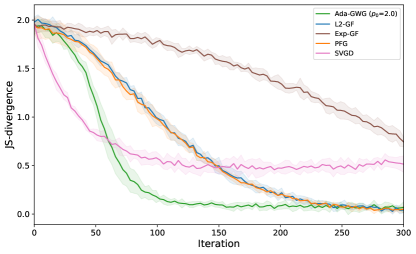
(a) JS divergence

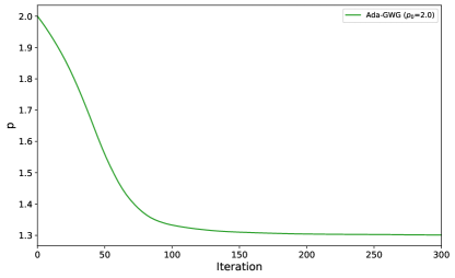
(b) Evolution of $\displaystyle p$

Figure 5: Quantitative results in Gaussian Mixture experiment

F.2 Monomial Gamma

On heavy tailed distributions, the number of particles is 1000. For GWG and Ada-GWG, the neural network structure is the same as which in the Gaussian mixture experiment. The inner loop iteration is also 5, but we use Adam optimizer with learning rate $\displaystyle\eta$=1e-3 to train $\displaystyle f_{w}$ for better stability. The particle step size is 1e-3.

For Ada-GWG, we set the initial exponent $\displaystyle p_{0}\in\{1.5,2.0,2.2\}$ and learning rate $\displaystyle\tilde{\eta}=1$.

We run the experiment on 4 random seeds. The average results and the variances are represented in the figure using lines and shades.

F.3 Conditioned Diffusion

The procedure to generate the true path is exactly the same as in Detommaso et al. [14]. For PFG and Ada-GWG, we parameterize $\displaystyle f_{w}$ as 3-layer neural networks with tanh nonlinearities. Each hidden layer has $\displaystyle 200$ neurons. The inner loop $\displaystyle N^{\prime}$ is selected from $\displaystyle\{1,5,10,15\}$ to get the best performance. $\displaystyle f_{w}$ is pre-trained for $\displaystyle 100$ iterations before particle updates and we use Adam optimizer with learning rate $\displaystyle\eta$=1e-3 to train $\displaystyle f_{w}$. The particle step size is $\displaystyle 3e-3$ for Ada-GWG and PFG.

For Ada-GWG, we set the initial exponent $\displaystyle p_{0}=2.2$ and learning rate $\displaystyle\tilde{\eta}=0.001$. The gradient of $\displaystyle A(p)$ is also clipped within $\displaystyle[-0.1,0.1]$.

For PFG, we set the preconditioning matrix $\displaystyle H={\hat{H}}^{\alpha}$, where $\displaystyle\hat{H}$ is the inverse of diagonal variance of particles and $\displaystyle\alpha$ is chosen from $\displaystyle\{0.1,0.5,1.0\}$ to obtain the best performance.

For SVGD, we use RBF kernel $\displaystyle\exp(-\frac{\|x-y\|^{2}}{h})$ where $\displaystyle h$ is the heuristic bandwidth [31]. The initial step size is 1e-3 and is adjusted by AdaGrad.

Additionally, we run LMC with step size 1e-4 for $\displaystyle 10000$ iterations as the ground truth for posterior distribution.

F.4 Bayesian Neural Networks

Our experiment settings are almost similar to SVGD [31]. For the UCI datasets, the datasets are randomly partitioned into 90% for training and 10% for testing. Then, we further split the training dataset by 10% to create a validation set for hyperparameter selection as done in [31]. For $\displaystyle L_{2}$-GF and Ada-GWG, we parameterize $\displaystyle f_{w}$ as 3-layer neural networks. Each hidden layer has $\displaystyle 300$ neurons, and we use LeakyReLU as the activation function with a negative slope of 0.1. The inner loop $\displaystyle N^{\prime}$ is selected from $\displaystyle\{1,5,10\}$. We use the Adam optimizer and choose the learning rate from $\displaystyle\{0.001,0.0001\}$ to train $\displaystyle f_{w}$.

For Ada-GWG, we choose the initial exponent $\displaystyle p_{0}$ from $\displaystyle\{3,4\}$ and set the learning rate $\displaystyle\tilde{\eta}=0.0001$. The gradient of $\displaystyle A(p)$ is clipped within [-0.2, 0.2]. We select the step size of particle updates from $\displaystyle\{0.0001,0.0002,0.0005,0.001\}$. For SVGD, we use the RBF kernel as done in [31]. For SVGD, $\displaystyle L_{2}$-GF, and Ada-GWG, the iteration number is chosen from $\displaystyle\{2000,4000\}$ to converge. For SGLD, the iteration number is set to 10000 to converge.

Appendix G Limitations and Future Work

Estimating Wasserstein gradient by neural networks.

Our formulation leverages the capability of neural networks to estimate the generalized Wasserstein gradient. This approach successfully resolves the problem of kernel design for conventional ParVI methods. However, in high dimensional regime, the design of neural network structure is still important but subtle. Besides, the computation cost is also expensive. We expect more efficient algorithms on training neural works to approximate Wasserstein gradient, e.g.Wang et al. [44].

Better adaptive method.

Our Ada-GWG method is based on the idea of maximizing the decent rate of KL divergence and heavily relies on an accurate estimation of generalized Wasserstein gradient. We update exponent $\displaystyle p$ by simply gradient ascent which may cause severe numerical instability. Although this can be alleviated by clipping, it is still delicate when the target distribution is complex.

General Young function class.

In this paper, we only consider the function class $\displaystyle\left\{\frac{1}{p}\|\cdot\|_{p}^{p}:p>1\right\}$, which is still limited. We expect a more general function class that both have numerical stability and can perfectly capture the information from score function. The characteristics of Young function class may be instructive. How to design an adaptive algorithm on a more general class is also challenging and important. We leave this to future research.

Shortness of theoretical analysis.

Although we provide convergence guarantee under weak assumptions, our analysis is still preliminary and we believe these results can be strengthened. There are also other important extensions to consider. For example, our analysis is based on the population loss, which is an asymptotic result based on infinite particles limit. We believe this framework can be also generalized to finite-particle system like SVGD [28]. Moreover, we only consider Young functions that have the form of $\displaystyle\|\cdot\|_{p}^{p}$ or are strongly convex and strongly smooth. We believe that better-designed Young functions may have more advantageous theoretical properties, e.g., Wasserstein Newton flow [43].

References

- Adamczak et al. [2017] Radosław Adamczak, Witold Bednorz, and Paweł Wolff. Moment estimates implied by modified log-sobolev inequalities. ESAIM: Probability and Statistics, 21:467–494, 2017.
- Alvarez-Melis et al. [2022] David Alvarez-Melis, Yair Schiff, and Youssef Mroueh. Optimizing functionals on the space of probabilities with input convex neural networks. Transactions on Machine Learning Research, 2022. ISSN 2835-8856. URL https://openreview.net/forum?id=dpOYN7o8Jm.
- Ambrosio et al. [2005] Luigi Ambrosio, Nicola Gigli, and Giuseppe Savaré. Gradient flows: in metric spaces and in the space of probability measures. Springer Science & Business Media, 2005.
- Balasubramanian et al. [2022] Krishnakumar Balasubramanian, Sinho Chewi, Murat A. Erdogdu, Adil Salim, and Matthew Shunshi Zhang. Towards a theory of non-log-concave sampling: First-order stationarity guarantees for langevin monte carlo. In Annual Conference Computational Learning Theory, 2022.
- Barp et al. [2019] Alessandro Barp, Francois-Xavier Briol, Andrew Duncan, Mark Girolami, and Lester Mackey. Minimum stein discrepancy estimators. Advances in Neural Information Processing Systems, 32, 2019.
- Barthe & Roberto [2008] Franck Barthe and Cyril Roberto. Modified logarithmic sobolev inequalities on. Potential Analysis, 29(2):167, 2008.
- Blei et al. [2016] David M. Blei, Alp Kucukelbir, and Jon D. McAuliffe. Variational inference: A review for statisticians. Journal of the American Statistical Association, 112:859 – 877, 2016.
- Bobkov & Ledoux [2000] Sergey G Bobkov and Michel Ledoux. From brunn-minkowski to brascamp-lieb and to logarithmic sobolev inequalities. Geometric and Functional Analysis, 10:1028–1052, 2000.
- Chen et al. [2018] Changyou Chen, Ruiyi Zhang, Wenlin Wang, Bai Li, and Liqun Chen. A unified particle-optimization framework for scalable bayesian sampling. ArXiv, abs/1805.11659, 2018.
- Chen et al. [2014] Tianqi Chen, Emily Fox, and Carlos Guestrin. Stochastic gradient hamiltonian monte carlo. In International Conference on Machine Learning, pp. 1683–1691, 2014.
- Chewi et al. [2020] Sinho Chewi, Thibaut Le Gouic, Chen Lu, Tyler Maunu, and Philippe Rigollet. Svgd as a kernelized wasserstein gradient flow of the chi-squared divergence. Advances in Neural Information Processing Systems, 33, 2020.
- Cui et al. [2016] Tiangang Cui, Kody JH Law, and Youssef M Marzouk. Dimension-independent likelihood-informed mcmc. Journal of Computational Physics, 304:109–137, 2016.
- Dalalyan & Karagulyan [2019] Arnak S Dalalyan and Avetik Karagulyan. User-friendly guarantees for the langevin monte carlo with inaccurate gradient. Stochastic Processes and their Applications, 129(12):5278–5311, 2019.
- Detommaso et al. [2018] Gianluca Detommaso, Tiangang Cui, Youssef Marzouk, Alessio Spantini, and Robert Scheichl. A stein variational newton method. Advances in Neural Information Processing Systems, 31, 2018.
- Devroye et al. [2018] Luc Devroye, Abbas Mehrabian, and Tommy Reddad. The total variation distance between high-dimensional gaussians. arXiv preprint arXiv:1810.08693, 6, 2018.
- di Langosco et al. [2021] Lauro Langosco di Langosco, Vincent Fortuin, and Heiko Strathmann. Neural variational gradient descent. ArXiv, abs/2107.10731, 2021.
- Dong et al. [2023] Hanze Dong, Xi Wang, LIN Yong, and Tong Zhang. Particle-based variational inference with preconditioned functional gradient flow. In The Eleventh International Conference on Learning Representations, 2023. URL https://openreview.net/forum?id=6OphWWAE3cS.
- Duane et al. [1987] S. Duane, A. D. Kennedy, B J. Pendleton, and D. Roweth. Hybrid Monte Carlo. Physics Letters B, 195(2):216 – 222, 1987.
- Fan et al. [2022] Jiaojiao Fan, Qinsheng Zhang, Amirhossein Taghvaei, and Yongxin Chen. Variational wasserstein gradient flow. In International Conference on Machine Learning, pp. 6185–6215. PMLR, 2022.
- Gentil et al. [2005] Ivan Gentil, Arnaud Guillin, and Laurent Miclo. Modified logarithmic sobolev inequalities and transportation inequalities. Probability theory and related fields, 133:409–436, 2005.
- Gentil et al. [2007] Ivan Gentil, Arnaud Guillin, and Laurent Miclo. Modified logarithmic sobolev inequalities in null curvature. Revista Matematica Iberoamericana, 23(1):235–258, 2007.
- Grathwohl et al. [2020] Will Grathwohl, Kuan-Chieh Wang, Jörn-Henrik Jacobsen, David Duvenaud, and Richard Zemel. Learning the stein discrepancy for training and evaluating energy-based models without sampling. In International Conference on Machine Learning, pp. 3732–3747. PMLR, 2020.
- Hu et al. [2018] Tianyang Hu, Zixiang Chen, Hanxi Sun, Jincheng Bai, Mao Ye, and Guang Cheng. Stein neural sampler. arXiv preprint arXiv:1810.03545, 2018.
- Hutchinson [1989] Michael F Hutchinson. A stochastic estimator of the trace of the influence matrix for laplacian smoothing splines. Communications in Statistics-Simulation and Computation, 18(3):1059–1076, 1989.
- Jordan et al. [1999] Michael I. Jordan, Zoubin Ghahramani, T. Jaakkola, and Lawrence K. Saul. An introduction to variational methods for graphical models. Machine Learning, 37:183–233, 1999.
- Jordan et al. [1998] Richard Jordan, David Kinderlehrer, and Felix Otto. The variational formulation of the fokker–planck equation. SIAM journal on mathematical analysis, 29(1):1–17, 1998.
- Koehler et al. [2023] Frederic Koehler, Alexander Heckett, and Andrej Risteski. Statistical efficiency of score matching: The view from isoperimetry. In The Eleventh International Conference on Learning Representations, 2023. URL https://openreview.net/forum?id=TD7AnQjNzR6.
- Korba et al. [2020] Anna Korba, Adil Salim, Michael Arbel, Giulia Luise, and Arthur Gretton. A non-asymptotic analysis for stein variational gradient descent. Advances in Neural Information Processing Systems, 33:4672–4682, 2020.
- Liu et al. [2019] Chang Liu, Jingwei Zhuo, Pengyu Cheng, Ruiyi Zhang, Jun Zhu, and Lawrence Carin. Understanding and accelerating particle-based variational inference. International Conference on Machine Learning. PMLR, pp. 4082-4092, 2019.
- Liu [2017] Qiang Liu. Stein variational gradient descent as gradient flow. Advances in neural information processing systems, 30, 2017.
- Liu & Wang [2016] Qiang Liu and Dilin Wang. Stein variational gradient descent: A general purpose bayesian inference algorithm. Advances in neural information processing systems, 29, 2016.
- Mou et al. [2022] Wenlong Mou, Nicolas Flammarion, Martin J Wainwright, and Peter L Bartlett. Improved bounds for discretization of langevin diffusions: Near-optimal rates without convexity. Bernoulli, 28(3):1577–1601, 2022.
- Mulholland [1949] HP Mulholland. On generalizations of minkowski’s inequality in the form of a triangle inequality. Proceedings of the London mathematical society, 2(1):294–307, 1949.
- Neal [2011] Radford Neal. MCMC using hamiltonian dynamics. In S Brooks, A Gelman, G Jones, and XL Meng (eds.), Handbook of Markov Chain Monte Carlo, Chapman & Hall/CRC Handbooks of Modern Statistical Methods. Taylor & Francis, 2011. ISBN 9781420079425. URL http://books.google.com/books?id=qfRsAIKZ4rIC.
- Newey & McFadden [1986] Whitney Newey and Daniel McFadden. Large sample estimation and hypothesis testing. Handbook of Econometrics, 4:2111–2245, 1986.
- Santambrogio [2017] Filippo Santambrogio. Euclidean, metric, and Wasserstein gradient flows: an overview. Bulletin of Mathematical Sciences, 7:87–154, 2017.
- Song et al. [2020] Yang Song, Sahaj Garg, Jiaxin Shi, and Stefano Ermon. Sliced score matching: A scalable approach to density and score estimation. In Uncertainty in Artificial Intelligence, pp. 574–584. PMLR, 2020.
- Vempala & Wibisono [2019] Santosh Vempala and Andre Wibisono. Rapid convergence of the unadjusted langevin algorithm: Isoperimetry suffices. In H. Wallach, H. Larochelle, A. Beygelzimer, F. d'Alché-Buc, E. Fox, and R. Garnett (eds.), Advances in Neural Information Processing Systems, volume 32. Curran Associates, Inc., 2019. URL https://proceedings.neurips.cc/paper_files/paper/2019/file/65a99bb7a3115fdede20da98b08a370f-Paper.pdf.
- Villani [2021] Cédric Villani. Topics in optimal transportation, volume 58. American Mathematical Soc., 2021.
- Villani et al. [2009] Cédric Villani et al. Optimal transport: old and new, volume 338. Springer, 2009.
- Wainwright & Jordan [2008] M. J. Wainwright and M. I. Jordan. Graphical models, exponential families, and variational inference. Foundations and Trends in Maching Learning, 1(1-2):1–305, 2008.
- Wang et al. [2018] Dilin Wang, Hao Liu, and Qiang Liu. Variational inference with tail-adaptive f-divergence. Advances in Neural Information Processing Systems, 31, 2018.
- Wang & Li [2020] Yifei Wang and Wuchen Li. Information newton’s flow: second-order optimization method in probability space. ArXiv, abs/2001.04341, 2020.
- Wang et al. [2022] Yifei Wang, Peng Chen, Mert Pilanci, and Wuchen Li. Optimal neural network approximation of wasserstein gradient direction via convex optimization. arXiv preprint arXiv:2205.13098, 2022.
- Welling & Teh [2011] Max Welling and Yee W Teh. Bayesian learning via stochastic gradient langevin dynamics. In International Conference on Machine Learning, pp. 681–688, 2011.
- Wibisono & Yang [2022] Andre Wibisono and Kay Yang. Convergence in kl divergence of the inexact langevin algorithm with application to score-based generative models. ArXiv, abs/2211.01512, 2022.