Solving and Applying Fractal Differential Equations: Exploring Fractal Calculus in Theory and Practice

Abstract

In this paper, we delve into the fascinating realm of fractal calculus applied to fractal sets and fractal curves. Our study includes an exploration of the method analogues of the separable method and the integrating factor technique for solving $\alpha$-order differential equations. Notably, we extend our analysis to solve Fractal Bernoulli differential equations. The applications of our findings are then showcased through the solutions of problems such as fractal compound interest, the escape velocity of the earth in fractal space and time, and the estimation of time of death incorporating fractal time. Visual representations of our results are also provided to enhance understanding.

Keywords: FFractal calculus, Fractal curves, Fractal differential equations
MSC: 28A80, 28A78, 28A35, 28A75, 34A30

1 Introduction

Benoit Mandelbrot is credited with pioneering the field of fractal geometry [1], which revolves around shapes possessing fractal dimensions that surpass their topological dimensions [2, 3]. These intricate fractals exhibit self-similarity and frequently demonstrate non-integer and complex dimensions [4, 5]. However, the analysis of fractals presents challenges, given that traditional geometric measures such as Hausdorff measure [6], length, surface area, and volume are typically applied to standard shapes [7]. Consequently, the direct application of these measures to fractal analysis becomes intricate [8, 9, 10, 11, 12, 13]. Researchers have tackled the problem of fractal analysis using approaches. These include analysis [14, 15], measure theory [16, 17, 18, 19, 20, 21, 22], probabilistic methods [23], fractional space and nonstandard methods [24], fractional calculus [25, 26, 27] and non standard methods [28]. Essential topological characteristics such as connectivity, ramification, and loopiness were exhibited by fractals and can be quantified using six independent dimension values. However, some fractal types may reduce the count of these dimensions due to their unique traits [29]. Fracture network modeling was proposed, with a specific focus on accentuating fractal attributes within geological formations. Two innovative models were introduced: one centered around Bernoulli percolation within regular lattices, and the other delving into site percolation within scale-free networks integrated into 2D and 3D lattices. The revelation emerged that the effective spatial degrees of freedom in scale-free networks are dictated by the embedding dimension, in contrast to the degree distribution [30]. The fractal characteristics impact percolation within self-similar networks [31]. The effects of geometric confinement on point statistics in a quasi-low-dimensional system were studied. Specifically, attention was centered on nearest-neighbor statistics. Comprehensive numerical simulations were carried out using binomial point processes on quasi-one-dimensional rectangle strips, considering various confinement ratio values. The findings revealed that the distributions of nearest-neighbor distances followed an extreme value Weibull distribution, where the shape parameter was contingent on the confinement ratio [32]. The fractal characteristics impact formation factors in pore-fracture networks for different transport processes. A focus on deterministic infinitely ramified networks related to pre-fractal Sierpinski carpets was adopted. The network attributes effects on streamline constriction and transmission path tortuosity, emphasizing formation factor differences for diffusibility, electrical conductivity, and hydraulic permeability [33]. Fractal calculus is a way to extend calculus and deal with equations that have solutions, in the form of functions with fractal properties like fractal sets and curves [34, 35]. The beauty of fractal calculus lies in its simplicity and algorithmic approaches when compared to methods [36]. The generalization of $F^{\alpha}$-calculus (FC) has been achieved through the utilization of the gauge integral method. The focus lies on the integration of functions within a subset of the real line containing singularities present in fractal sets [37]. The utilization of FC is exemplified with respect to fractal interpolation functions and Weierstrass functions, which can exhibit non-differentiability and non-integrability in the context of ordinary calculus [38]. The utilization of non-local fractal derivatives to characterize fractional Brownian motion on thin Cantor-like sets was demonstrated. The proposal of the fractal Hurst exponent establishes its connection to the order of non-local fractal derivatives [39]. Various methods have been employed to solve fractal differential equations, and their stability conditions have been determined [40, 41]. The fractal Tsallis entropy on fractal sets and defines q-fractal calculus for deriving distributions were introduced. Nonlinear coupling conditions for statistical states were presented, and a relationship between fractal dimension and Tsallis entropy’s q-parameter in the Hadron system was proposed [42]. Fractal functional differential equations were introduced as a mathematical framework for phenomena that encompass both fractal time and structure. The paper showcases the solution of fractal retarded, neutral, and renewal delay differential equations with constant coefficients, employing the method of steps and Laplace transforms [43]. The introduction of a novel generalized local fractal derivative operator and its exploration in classical systems via Lagrangian and Hamiltonian formalisms were undertaken. The practical applicability of the variational method in describing dissipative dynamical systems was showcased, and the Hamiltonian approach produced auxiliary constraints without reliance on Dirac auxiliary functions [44]. Furthermore, fractal stochastic differential equations have been defined, with categorizations for processes like fractional Brownian motion and diffusion occurring within mediums with fractal structures [45, 46, 47, 48, 49]. Local vector calculus within fractional-dimensional spaces, on fractals, and in fractal continua was developed. The proposition was put forth that within spaces characterized by non-integer dimensions, it was feasible to define two distinct del-operators-each operating on scalar and vector fields. Employing these del-operators, the foundational vector differential operators and Laplacian in fractional-dimensional space were formulated in a conventional manner. Additionally, Laplacian and vector differential operators linked with $F^{\alpha}$-derivatives on fractals were established [50]. Fractal calculus has been extended to include Cantor cubes and Cantor tartan [51], and the Laplace equation has been defined within this framework [52].
The paper is structured as follows:
In Section 2, a comparative and review analysis of fractal calculus is presented, focusing on its application to both fractal sets and curves. Section 3 introduces the utilization of an integrating factor to solve fractal $\alpha$-order differential equations. Section 4 outlines the application of the method of separation to fractal differential equations. Furthermore, in Section 5, various applications are discussed, involving the extension of standard models to account for fractal time. Lastly, Section 6 is dedicated to concluding the paper.

2 Overview of Fractal Calculus

In this section, we present a comprehensive survey of the application of fractal calculus to the domains of fractal curves and fractal sets [34, 35, 36].

2.1 Fractal Calculus on Fractal Sets

In this section, we present a concise overview of fractal calculus applied to fractal sets as summarized in [34].

Definition 2.1

The flag function of a set $F$ and a closed interval $I$ is defined as:

$$\rho(F,I)=\begin{cases}1,&\text{if }F\cap I\neq\emptyset;\\ 0,&\text{otherwise}.\end{cases}$$ (1)

Definition 2.2

For a fractal set $F\subset[a,b]$, a subdivision $P_{[a,b]}$ of $[a,b]$, and a given $\delta>0$, the coarse-grained mass of $F\cap[a,b]$ is defined by

$$\gamma_{\delta}^{\alpha}(F,a,b)=\inf_{|P|\leq\delta}\sum_{i=0}^{n-1}\Gamma(\alpha+1)(t_{i+1}-t_{i})^{\alpha}\rho(F,[t_{i},t_{i+1}]),$$ (2)

where $|P|=\max_{0\leq i\leq n-1}(t_{i+1}-t_{i})$, and $0<\alpha\leq 1$.

Definition 2.3

The mass function of a fractal set $F\subset[a,b]$ is defined as the limit of the coarse-grained mass as $\delta$ approaches zero:

$$\gamma^{\alpha}(F,a,b)=\lim_{\delta\rightarrow 0}\gamma_{\delta}^{\alpha}(F,a,b).$$ (3)

Definition 2.4

For a fractal set $F\subset[a,b]$, the $\gamma$-dimension of $F\cap[a,b]$ is defined as:

$$\dim_{\gamma}(F\cap[a,b]) =\inf\{\alpha:\gamma^{\alpha}(F,a,b)=0\}$$

$$=\sup\{\alpha:\gamma^{\alpha}(F,a,b)=\infty\}$$ (4)

Definition 2.5

The integral staircase function of order $\alpha$ for a fractal set $F$ is given by:

$$S_{F}^{\alpha}(x)=\begin{cases}\gamma^{\alpha}(F,a_{0},x),&\text{if }x\geq a_{0};\\ -\gamma^{\alpha}(F,x,a_{0}),&\text{otherwise}.\end{cases}$$ (5)

where $a_{0}$ is an arbitrary fixed real number.

Definition 2.6

Let $F$ be an $\alpha$-perfect fractal set, let $f$ be a function defined on F and let $x\in F.$ The $F^{\alpha}$-derivative of $f$ at the point $x$ is defined as follows:

$$D_{F}^{\alpha}f(x)=\begin{cases}\underset{y\rightarrow x}{F_{-}\text{lim}}~{}\frac{f(y)-f(x)}{S_{F}^{\alpha}(y)-S_{F}^{\alpha}(x)},&\text{if }x\in F;\\ 0,&\text{otherwise}.\end{cases}$$ (6)

if the fractal limit $F_{-}\text{lim}$ exists [34].

Definition 2.7

Let $I=[a,b]$. Let $F$ be an $\alpha$-perfect fractal set such that $S^{\alpha}_{F}$ is finite on $I$. Let $f$ be a bounded function defined on F and let $x\in F.$ The $F^{\alpha}$-integral of $f$ on $I$ is defined as:

$$\int_{a}^{b}f(x)d_{F}^{\alpha}x =\sup_{P_{[a,b]}}\sum_{i=0}^{n-1}\inf_{x\in F\cap I}f(x)(S_{F}^{\alpha}(x_{i+1})-S_{F}^{\alpha}(x_{i}))$$

$$=\inf_{P_{[a,b]}}\sum_{i=0}^{n-1}\sup_{x\in F\cap I}f(x)(S_{F}^{\alpha}(x_{i+1})-S_{F}^{\alpha}(x_{i})).$$ (7)

2.2 Fractal Calculus on Fractal Curves

We begin with defining the key concepts in fractal calculus on fractal curves [35]. By the way, we recall that a fractal curve $F\subset\mathbb{R}^{n}$ is parametrizable if there exists a bijective and continuous function $\mathbf{w}:[a_{0},b_{0}]\rightarrow\mathbb{R}$. Moreover we recall also that by $C(a,b)$ we denote the segment of the curve lying between the points $\mathbf{w}(a)$ and $\mathbf{w}(b)$ on the fractal curve $F$ [35].

Definition 2.8

For a fractal curve denoted as $F$ and a subdivision denoted as $P_{[a,b]}$ where $[a,b]\subset\mathbb{R}$, the mass function is given by

$$\gamma^{\alpha}(F,a,b)=\lim_{\delta\rightarrow 0}\inf_{|P|\leq\delta}\sum_{i=0}^{n-1}\frac{|\mathbf{w}(t_{i+1})-\mathbf{w}(t_{i})|^{\alpha}}{\Gamma(\alpha+1)},$$ (8)

where $|\cdot|$ represents the Euclidean norm in $\mathbb{R}^{n}$, $1\leq\alpha\leq n$, $P_{[a,b]}=\{a=t_{0},...,t_{n}=b\}$, and $|P|=\max_{0\leq i\leq n-1}(t_{i+1}-t_{i})$ for a subdivision $P_{[a,b]}$.

Definition 2.9

The $\gamma$-dimension of the fractal curve $F$ is defined as

$$\dim_{\gamma}(F) =\inf\{\alpha:\gamma^{\alpha}(F,a,b)=0\}$$

$$=\sup\{\alpha:\gamma^{\alpha}(F,a,b)=\infty\}$$ (9)

Definition 2.10

Let $p_{0}\in[a_{0},b_{0}]$ be arbitrary but fixed. The mass of the fractal of a fractal curve $F$ is defined as:

$$S_{F}^{\alpha}(u)=\begin{cases}\gamma^{\alpha}(F,p_{0},u),&u\geq p_{0};\\ -\gamma^{\alpha}(F,u,p_{0}),&u<p_{0}.\end{cases}$$ (10)

The mass of the fractal curve $F$ up to point $u$ is provided by $S_{F}^{\alpha}(u)$, where $u\in[a_{0},b_{0}].$

Definition 2.11

Let $S^{\alpha}_{F}(u)=J(\theta).$ The fractal $F^{\alpha}$-derivative of a function $f$ at a point $\theta\in F$ is defined as:

$$D_{F}^{\alpha}f(\theta)=\underset{\theta^{\prime}\rightarrow\theta}{F_{-}lim}~{}\frac{f(\theta^{\prime})-f(\theta)}{J(\theta^{\prime})-J(\theta)},$$ (11)

if $F_{-}lim$ exists (here the $F_{-}lim$ represents the fractal limit as it shows in [35]).

Remark 1

It is worth noting that the Euclidean distance from the origin to a point $\theta=\mathbf{w}(u)$ is given by $L(\theta)=L(\mathbf{w}(u))=|\mathbf{w}(u)|.$

Definition 2.12

The fractal integral or $F^{\alpha}$-integral is defined as

$$\int_{C(a,b)}f(\theta)d_{F}^{\alpha}\theta =\sup_{P[a,b]}\sum_{i=0}^{n-1}\inf_{\theta\in C(t_{i},t_{i+1})}f(\theta)(J(\theta_{i+1})-J(\theta_{i}))$$

$$=\inf_{P[a,b]}\sum_{i=0}^{n-1}\sup_{\theta\in C(t_{i},t_{i+1})}f(\theta)(J(\theta_{i+1})-J(\theta_{i})),$$ (12)

where $t_{i}=\mathbf{w}^{-1}(\theta_{i})$ and $f$ is a bounded function on a fractal curve $F$.

3 Solving Fractal Differential Equations by Method of Integrating Factor

In this section, we delve into the concept of differential equations on fractal curves and fractal sets. We start by considering an $\alpha$-order linear differential equation on a fractal curve $F\subset\mathbb{R}^{n}$:

$$D_{F}^{\alpha}y(\theta)+p(\theta)y(\theta)=g(\theta),~{}~{}~{}\theta\in F,$$ (13)

where $p$ and $g$ are $F$-continuous functions defined on the fractal curve $F$, with $\varphi_{1}<\theta<\varphi_{2}$, and $\varphi_{1},\varphi_{2}\in F$.

Definition 1

Let $\psi:F\subset\mathbb{R}^{n}\rightarrow\mathbb{R}$ be a function. If $\psi$ has fractal $F^{\alpha}$-derivative at each point $\theta\in F,$ therefore $\psi$ is called the solution of the $\alpha$-order differential equation if substituted in the Eq.(13) satisfies it.

Theorem 1

(Method of the integration factor)

Let $F\subset\mathbb{R}^{n}$ be a fractal curve, therefore there exists a fractal $F^{\alpha}$-differentiable function defined on a fractal curve $F,$ called integration factor, such that all the solutions of the Eq. Eq.(13) are expressed by:

$$y(\theta)=\frac{\int\mu(\theta)g(\theta)d^{\alpha}_{F}(\theta)\,+\,J(c)}{\mu(\theta)}.$$ (14)

Here $\mu(\theta)$ is the integration factor and $J(c)$ is an arbitrary constant.

Proof 1

To solve Eq. (13), we introduce an integrating factor $\mu(\theta)$ and multiply both sides of the equation by it:

$$\mu(\theta)D_{F}^{\alpha}y(\theta)+\mu(\theta)p(\theta)y(\theta)=\mu(\theta)g(\theta).$$ (15)

For this modified equation to hold, we require the following relationship:

$$D_{F}^{\alpha}\mu(\theta)=p(\theta)\mu(\theta).$$ (16)

Assuming $\mu(\theta)>0$, we can express Eq. (16) as:

$$\frac{D_{F}^{\alpha}\mu(\theta)}{\mu(\theta)}=p(\theta).$$ (17)

By applying fractal integration, we arrive at the integral equation:

$$\ln(\mu(\theta))=\int p(\theta)d_{F}^{\alpha}\theta+J(k),$$ (18)

where $J(k)$ is an arbitrary constant of integration. Setting $J(k)=0$, we obtain the expression for the integrating factor:

$$\mu(\theta)=\exp\left(\int p(\theta)d_{F}^{\alpha}\theta\right).$$ (19)

After determining $\mu(\theta)$, we substitute it back into Eq. (15), yielding:

$$D_{F}^{\alpha}(\mu(\theta)y(\theta))=\mu(\theta)g(\theta).$$ (20)

Integrating both sides of the equation using fractal integration, we arrive at the solution for the original differential equation (13):

$$y(\theta)=\frac{\int\mu(\theta)g(\theta)d_{F}^{\alpha}\theta+J(c)}{\mu(\theta)},$$ (21)

which completes the proof.

Remark 2

By the previous theorem it follows that there are infinitely many functions $y(\theta)$ that satisfy the given $\alpha$-order fractal differential equation on the fractal curve $F$.

Example 1

Consider an $\alpha$-order fractal differential equation on fractal curve $F$ of the form:

$$D_{F}^{\alpha}y(\theta)=ry(\theta)+k,$$ (22)

where $r$ and $k$ are constants. By Equation (21), we can determine the infinite solutions for the given equations (22) as follows:

$$y(\theta)=-\frac{k}{r}+c\exp(rJ(\theta)),$$ (23)

where $c$ is an integration constant, and $J(\theta)$ arises from the fractal integration process.

Theorem 2

Let $p(\theta)$ and $g(\theta)$ two $F$-continuous functions defined on a fractal curve $F$ with $\varphi_{1}<\theta<\varphi_{2}$ and $\varphi_{1},\varphi_{2}\in F.$ Let $\theta_{0}\in(\varphi_{1},\varphi_{2})$. Therefore for each $y_{0}\in\mathbb{R}$ there exists an unique solution $y=\psi(\theta)$, defined at least in a neighborhood of $\theta_{0}$, of the following $\alpha$-order fractal differential equation:

$$D^{\alpha}_{F}y(\theta)+p(\theta)y(\theta)=g(\theta),$$ (24)

with the initial condition $y(\theta_{0})=y_{0}.$

Proof 2

Let us denote by $\Lambda(\theta)$ a primite of $p(\theta)$. The existence of a solution of the given $\alpha$-order fractal differential equation it was already shown by the method of the integration factor already discussed. Therefore, denoted by $\mu(\theta)=e^{\Lambda(\theta)}$ we arrive at:

$$y(\theta)=\,e^{-\Lambda(\theta)}\left(\int\ g(\theta)\,\mu(\theta)\,d^{\alpha}_{F}(\theta)\,+\,c\right),$$ (25)

where $c$ is a constant of integration. Now, replacing the initial condition $y(\theta_{0})=y_{0}$ in the previous equation and choosing the primitive $\Lambda(\theta)$ such that $\Lambda(\theta_{0})=0,\ (i.e.\ \Lambda(\theta)=\int_{C(\theta_{0},\theta)}\,p(\tau)d^{\alpha}_{F}\tau)$ we get the following solution:

$$y(\theta)=\ \,e^{-\Lambda(\theta)}\left(\int_{C(\theta_{0},\theta)}\mu(\tau)g(\tau)d^{\alpha}_{F}\tau\ +\,y_{0}\right).$$ (26)

To prove the uniqueness of the solution, let us suppose by contradiction that there are two different solutions $y_{1}(\theta)$ and $y_{2}(\theta)$ of the Eq.(24) with the same initial condition $y_{1}(\theta_{0})=y_{2}(\theta_{0})=y_{0}$.
Let $z(\theta)=y_{1}(\theta)-y_{2}(\theta)$. Therefore, by the linearity of the $\alpha$-order differential equation, substituting $z(\theta)$ into Eq. (24), we obtain:

$$D^{\alpha}_{F}z(\theta)\,+\,p(\theta)z(\theta)=0.$$ (27)

Now, it is trivial to observe that the function $z(\theta)=0,$ identically null, is a solution of $D^{\alpha}_{F}z(\theta)\,+\,p(\theta)z(\theta)=0$ with the initial condition $z(\theta_{0})=0.$ So, by the conjugacy of $F^{\alpha}$-calculus and the ordinary calculus [35], we can conclude that $z(\theta)=0$ is the unique solution of

$$D^{\alpha}_{F}z(\theta)\,+\,p(\theta)z(\theta)=0,$$ (28)

with the initial condition $z(\theta_{0})=0.$ Therefore, by the definition of $z(\theta)$ we have that $y_{1}(\theta)=y_{2}(\theta)$ and this is a contradiction having assumed that Eq.(24), with the initial condition $y(\theta_{0})=0,$ could admit two different solutions.

Example 2

Consider the fractal differential equation on a fractal set, expressed as

$$D_{t}^{\alpha}y(t)+\frac{1}{2}y(t)=10+5\sin(2S_{F}^{\alpha}(t))$$ (29)

where the initial condition is given as $y(0)=0$. To solve Eq.(29), we introduce the integrating factor $\mu(t)=\exp(S_{F}^{\alpha}(t)/2)$. By multiplying Eq.(29) with this factor, performing fractal integration, and applying the initial condition, the resulting solution is:

$$y(t) =20-\frac{40}{17}\cos(2S_{F}^{\alpha}(t))+\frac{10}{17}\sin(2S_{F}^{\alpha}(t))-\frac{300}{17}\exp\left(-\frac{S_{F}^{\alpha}(t)}{2}\right)$$

$$\propto 20-\frac{40}{17}\cos(2t^{\alpha})+\frac{10}{17}\sin(2t^{\alpha})-\frac{300}{17}\exp\left(-\frac{t^{\alpha}}{2}\right).$$ (30)

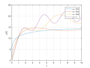
Figure 1: Plot of Eq.(2) for different values of $\alpha$

In Figure 1, we have plotted Eq. (2) for various values of $\alpha$. This plot illustrates that as the dimension of the fractal set supporting the function increases, the solution exhibits greater oscillations.

3.1 Fractal Bernoulli Differential Equation

The fractal version of the Bernoulli differential equation, using the fractal derivative, is expressed as:

$$D_{F}^{\alpha}y(\theta)+q(\theta)y(\theta)=r(\theta)y(\theta)^{\beta},~{}~{}~{}\theta\in F,~{}\beta\in\mathbb{R},$$ (31)

where $q(\theta)$ and $r(\theta)$ are $F$-continuous functions defined on a fractal curve. This equation employs the fractal derivative to describe the behavior of the function $y$ on a fractal curve, allowing for the analysis and solution of differential equations on fractal geometries. In order to give a technique to solve the assigned Fractal Bernoulli differential equation, let us observe, first of all, that if $\beta=0$ then $y^{\beta}(\theta)=y^{0}(\theta)=1$ and the Eq.(31) becomes equal to the Eq.(13) with $r(\theta)=g(\theta).$ Instead, if $\beta=1$, then $y^{\beta}(\theta)=y(\theta)$ and the Eq.(31) becomes similar to the Eq.(13), here $q(\theta)-r(\theta)=p(\theta).$ In all other cases, to solve the fractal version of the Bernoulli differential equation, using fractal derivatives, we apply the integrating factor method already discussed. Before showing this technique we note that if $\beta>0,$ then $y(\theta)=0$ is a solution of the Eq.(31). Now, the solution method is the following: preliminarily divide both sides of the equation by $y^{\beta}(\theta)$, thus obtaining

$$y^{-\beta}(\theta)\left(D^{\alpha}_{F}y(\theta)\,+\,q(\theta)\,y(\theta)\right)\,=\,r(\theta),$$ (32)

subsequently set $z(\theta)=y^{1-\beta}(\theta)$ and applying the fractal differentiation rule of composite functions: $D^{\alpha}_{F}z(\theta)=(1-\beta)\,y^{-\beta}(\theta)\,D^{\alpha}_{F}y(\theta),$ so the new Fractal Bernoulli differential equation is

$$D^{\alpha}_{F}z(\theta)\,+\,(1-\beta)\,q(\theta)\,z(\theta)\,=\,(1-\beta)\,r(\theta).$$ (33)

Therefore apply the integrating factor method and set $y(\theta)=\left(z(\theta)\right)^{\frac{1}{1-\beta}},$ so the solution of the assigned Fractal Bernoulli differential equation is:

$$y(\theta)=\left(\frac{\int r(\theta)\,\mu(\theta)\,d^{\alpha}_{F}(\theta)\,+\,c}{\mu(\theta)}\right)^{\frac{1}{1-\beta}},$$ (34)

where $\Lambda(\theta)$ is a primite of $q(\theta)$ and $\mu(\theta)=e^{\Lambda(\theta)}.$

Example 3

Let us consider the following Fractal Bernoulli differential equation on a given fractal curve $F$:

$$D^{\alpha}_{F}y(\theta)\,=\,2\,\frac{y(\theta)}{S^{\alpha}_{F}(\theta)}\,+\,2\,S^{\alpha}_{F}(\theta)\,\sqrt{y(\theta)}$$

here $\beta=1/2,$ so $y(\theta)=0$ is a solution of the given Fractal Bernoulli differential equation. Let us suppose, now, that $y(\theta)\neq 0.$ Let us divide both sides of the equation by $\sqrt{y(\theta)}$ and let us set $z(\theta)=\sqrt{y(\theta)}.$ Thus we obtain the following $\alpha$-order linear differential equation on a given fractal curve $F$:

$$D^{\alpha}_{F}z(\theta)=S^{\alpha}_{F}(\theta)+\frac{z(\theta)}{S^{\alpha}_{F}(\theta)}$$ (35)

According to the formula of the integrating factor method we have:

$$z(\theta)=S^{\alpha}_{F}(\theta)(S^{\alpha}_{F}(\theta)\,+\,c).$$ (36)

Therefore the solutions of the assigned Fractal Bernoulli differential equation are: $y(\theta)=\left((S^{\alpha}_{F}(\theta))^{2}+c\,S^{\alpha}_{F}(\theta)\right)^{2}$ and $y(\theta)=0.$

4 Solving Fractal Differential Equations by Method of Separation

The equation representing a separable $\alpha$-order fractal differential equation is given as [53]:

$$D_{F}^{\alpha}y(\theta)=\frac{d_{F}^{\alpha}y}{d_{F}^{\alpha}\theta}=f(\theta,y),~{}~{}~{}\theta\in F,$$ (37)

with the initial condition

$$y(\theta_{0})=y_{0}.$$ (38)

Here, $f(\theta,y)$ takes a linear form with respect to $y$. The equation (37) can be rearranged as:

$$M(\theta,y)+N(\theta,y)\frac{d_{F}^{\alpha}y}{d_{F}^{\alpha}\theta}=0,$$ (39)

where $M(\theta,y)=-f(\theta,y)$ and $N(\theta,y)=1$. By considering $M(\theta,y)=M(\theta)$ and $N(\theta,y)=N(y)$, we arrive at:

$$M(\theta)d_{F}^{\alpha}\theta+N(y)d_{F}^{\alpha}y=0.$$ (40)

This equation is referred to as a separable fractal differentiable equation. To solve (40), we introduce functions $D_{F}^{\alpha}H_{1}(\theta)=M(\theta)$ and $D_{F}^{\alpha}H_{2}(y)=N(y)$. Therefore Eq. (40) has the following expression:

$$D_{F}^{\alpha}H_{1}(\theta)+D_{F}^{\alpha}H_{2}(y)\frac{d_{F}^{\alpha}y}{d_{F}^{\alpha}\theta}=0.$$ (41)

Now by fractal chain rule, we have:

$$D_{F}^{\alpha}H_{2}(y)\frac{d_{F}^{\alpha}y}{d_{F}^{\alpha}\theta}=\frac{d_{F}^{\alpha}}{d_{F}^{\alpha}\theta}H_{2}(y).$$ (42)

Consequently, by Eq. (41) and Eq. (42) we have:

$$\frac{d_{F}^{\alpha}}{d_{F}^{\alpha}\theta}[H_{1}(\theta)+H_{2}(y)]=0,$$ (43)

and applying fractal integration, we obtain:

$$H_{1}(\theta)+H_{2}(y)=c$$ (44)

The Eq.(44) is the implicit solution of the Eq.(40). Now by substituting the initial condition into Eq.(44) we get:

$$c=H_{1}(\theta_{0})+H_{2}(y_{0}).$$ (45)

Finally by replacing (45) into (44), we arrive at:

$$H_{2}(y)-H_{2}(y_{0})=\int_{y_{0}}^{y}N(s)d_{F}^{\alpha}s,~{}~{}~{}H_{1}(\theta)-H_{1}(\theta_{0})=\int_{C(\theta_{0},\theta)}M(s)d_{F}^{\alpha}s$$ (46)

This leads to:

$$\int_{y_{0}}^{y}N(s)d_{F}^{\alpha}s+\int_{C(\theta_{0},\theta)}M(s)d_{F}^{\alpha}s=0$$ (47)

which is the implicit solution of (40), satisfying the initial condition.

Example 4

Let’s consider the fractal differential equation on a fractal curve given by

$$D_{F}^{\alpha}y(\theta)=\frac{3J(\theta)^{2}+4J(\theta)+2}{2(y-1)},~{}~{}~{}y(0)=-1.$$ (48)

We can rewrite Eq.(48) as follows:

$$2(y-1)d_{F}^{\alpha}y=(3J(\theta)^{2}+4J(\theta)+2)d_{F}^{\alpha}\theta.$$ (49)

Moreover, by fractal integration with respect to $y$ on the left side and with respect to $\theta$ on the right side, we obtain:

$$y^{2}-2y=J(\theta)^{3}+2J(\theta)^{2}+2J(\theta)+c.$$ (50)

Finally, by using the initial condition $y(0)=-1$ in Eq. (50) we get:

$$y^{2}-2y=J(\theta)^{3}+2J(\theta)^{2}+2J(\theta)+3.$$ (51)

It can be further simplified to:

$$y(\theta)=1-\sqrt{J(\theta)^{3}+2J(\theta)^{2}+2J(\theta)+4}.$$ (52)

Figure 2: Graph of Eq.(52).

In Figure 2, we have depicted the graphical representation of the solution to equation (48).

5 Applications

In this section, we explore practical applications of fractal differential equations.

5.1 Fractal Compound Interest

Consider a scenario where a sum of money is deposited in a bank, and both deposits and withdrawals occur at a constant rate $k$ [54]. The value $p(t)$ of the investment over time represents this situation. The rate of change of $p(t)$ in a fractal time context is given by the equation:

$$D_{F}^{\alpha}p(t)=rp(t)+k,~{}~{}~{}~{}~{}~{}~{}t\in F,~{}~{}~{}r,k\in\mathbb{R}.$$ (53)

Here, $r$ represents the annual interest rate and $k$ the constant rate of deposits or withdrawals. The initial condition is $p(0)=p_{0}$. The solution to Eq.(53) is derived as:

$$p(t) =p_{0}\exp(rS_{F}^{\alpha}(t))+\frac{k}{r}(\exp(rS_{F}^{\alpha}(t)-1))$$ (54)

$$\propto p_{0}\exp(rt^{\alpha})+\frac{k}{r}(\exp(rt^{\alpha}-1)).$$ (55)

This solution showcases how the investment’s value changes over fractal time, with implications for compound interest calculations.

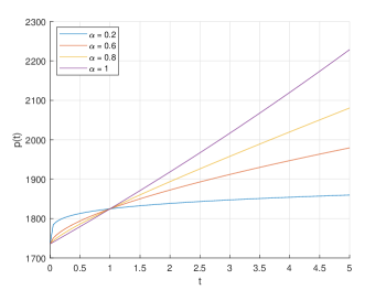
Figure 3: Investment growth for different values of $\alpha$

In Figure 3, we illustrate the impact of the fractal time dimension on the growth of investment.

5.2 Escape Velocity in Fractal Space and Time

The concept of escape velocity, a fundamental aspect of physics, pertains to the minimum initial velocity required for an object to overcome a celestial body’s gravitational pull [54]. By introducing the concept of fractal space and time, we extend the exploration of escape velocity to an innovative framework.
Assuming the absence of other forces and incorporating Newton’s law, the equation of motion in fractal space and time can be expressed as:

$$mD_{t}^{\alpha}v=-\frac{mgR^{2}}{(R+x)^{2}},~{}~{}~{}v(0)=0.$$ (56)

Here, $m$ represents the mass of the object, $R$ is the radius of the celestial body (such as Earth), $x$ is the distance between the object and the celestial body, and $g$ signifies the acceleration due to gravity. The equation (56) is then transformed using the fractal chain rule to obtain:

$$vD_{x}^{\alpha}v=-\frac{gR^{2}}{(R+x)^{2}}.$$ (57)

Solving this equation involves separating variables and performing fractal integration, resulting in the equation:

$$\frac{S_{F}^{\alpha}(v)^{2}}{2}=\frac{gR^{2}}{R+S_{F}^{\alpha}(x)}+c.$$ (58)

Utilizing the initial conditions $x=0$ and $v=v_{0}$, the maximum altitude reached by the object can be determined as:

$$x_{\text{max}}=\frac{S_{F}^{\alpha}(v_{0})^{2}R}{2Rg-S_{F}^{\alpha}(v_{0})^{2}}.$$ (59)

To find the initial velocity $S_{F}^{\alpha}(v_{0})$ required to elevate the object to the altitude $x_{\text{max}}$, the equation $S_{F}^{\alpha}(v)=0$ is employed, yielding:

$$S_{F}^{\alpha}(v_{0})=\sqrt{2gR\frac{x_{\text{max}}}{R+x_{\text{max}}}}.$$ (60)

As the concept of escape velocity extends to fractal space, the fractal escape velocity $S_{F}^{\alpha}(v_{e})$ is determined by allowing $x_{\text{max}}$ to approach infinity:

$$S_{F}^{\alpha}(v_{e})=\sqrt{2gR},$$ (61)

or equivalently,

$$v_{e}\propto(2gR)^{1/2\alpha}.$$ (62)

This study delves into the idea of escape velocity within the context of fractal space and time, offering fresh perspectives on the dynamics of entities in dimensions marked by intricacy and self-replication.

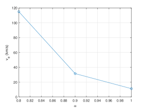
Figure 4: Escape Velocity vs. $\alpha$

As illustrated in Figure 4, we observe a pattern where reducing the spatial dimension necessitates an increase in escape velocity.

5.3 Fractal Newton’s Law of Cooling

Newton’s Law of Cooling is a fundamental principle in thermodynamics and heat transfer that describes how the rate of heat transfer between an object and its surroundings changes over time. It’s commonly used to model the cooling or heating of an object through conduction, convection, or radiation [55, 56].
The concept of the fractal Newton’s Law of Cooling can be presented in the following manner:

$$D_{t}^{\alpha}T=-k(T-T_{s}).$$ (63)

Where:

$$D_{t}^{\alpha}T~{}\text{signifies the fractal time derivative of temperature,}$$

$$T\text{ is the temperature of the object at any given time,}$$

$$T_{s}\text{ is the temperature of the surrounding environment,}$$

$$k>0\text{ is the cooling or heating rate coefficient.}$$

In this context, the rate of temperature change with respect to time is described through a fractal time derivative. This approach provides a unique lens through which to comprehend how objects interact with their surroundings, considering the intricacies of fractal time.

Estimation of Time of Death

As an example, let’s estimate the time of death for a body. We assume that the temperature of the body is discovered at time $t=0$ as $T_{0}$, and when it died at $t_{d}$, the temperature was $T_{d}$. By utilizing the cooling law, we can determine $t_{d}$ by solving Eq. (63), which can be represented as:

$$T(t)=T_{s}+(T_{0}-T)\exp(-kS_{F}^{\alpha}(t)).$$ (64)

Here, $T(0)=T_{0}$. If we measure the temperature of the deceased body at time $t=t_{1}$ and find $T=T_{1}$, we can use Eq. (63) to derive the equation:

$$T_{1}-T_{s}=(T_{0}-T)\exp(-kS_{F}^{\alpha}(t_{1})).$$ (65)

From this equation, we can deduce:

$$k=-\frac{1}{S_{F}^{\alpha}(t_{1})}\ln\frac{T_{1}-T_{s}}{T_{0}-T_{s}}\propto-\frac{1}{t_{1}^{\alpha}}\ln\frac{T_{1}-T_{s}}{T_{0}-T_{s}}.$$ (66)

By substituting $t=t_{d}$ and $T=T_{d}$ in the Eq. (64), we have:

$$S_{F}^{\alpha}(t_{d})=-\frac{1}{k}\ln\frac{T_{d}-T_{s}}{T_{0}-T_{s}}.$$ (67)

This equation can also be written as:

$$t_{d}=\bigg{|}-\frac{1}{k}\ln\frac{T_{d}-T_{s}}{T_{0}-T_{s}}\bigg{|}^{1/\alpha}.$$ (68)

This methodology provides a means for estimating the time of death based on temperature measurements and the principles of the fractal Newton’s Law of Cooling.

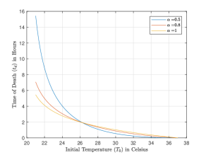
Figure 5: Estimation of Time of Death for Different $\alpha$ Values

Figure 5 illustrates that during the initial 2 hours, the cooling rate of the deceased body is faster in the fractal time model compared to the standard time case. However, this trend reverses beyond the 2-hour mark.

6 Conclusion

In conclusion, the study delved into a comprehensive exploration of various methods in the realm of fractal calculus. By investigating the method analogues of the separable method and integrating factor technique, we addressed $\alpha$-order differential equations. An intriguing extension of our analysis led to the resolution of Fractal Bernoulli differential equations, further broadening the scope of our inquiry. The practical implications of our findings were exemplified through their applications in solving real-world problems. From fractal compound interest to the escape velocity of earth in fractal space and time, and even the estimation of time of death with the incorporation of fractal time, our research showcased the versatility of fractal calculus in tackling complex scenarios. To enhance the accessibility of our work, we provided visual representations of our results. These aids not only conveyed our findings more effectively but also aided in the deeper understanding of the intricate concepts discussed. A holistic perspective on the applications of fractal calculus has been offered, demonstrating its adaptability and utility in solving diverse problems across various fields.
Declaration of Competing Interest:
The authors declare that they have no known competing financial interests or personal relationships that could have appeared to influence the work reported in this paper.
CRediT author statement:
Alireza.K.Golmankhnaeh : Investigation, Methodology, Software, Writing- Original draft preparation. Donatella Bongiorno : Investigation, Writing- Reviewing and Editing.
Declaration of generative AI and AI-assisted technologies in the writing process. During the preparation of this work the authors used GPT in order to correct grammar and writing. After using this GPT, the authors reviewed and edited the content as needed and takes full responsibility for the content of the publication.

7 References

References

- [1] B. B. Mandelbrot, The Fractal Geometry of Nature, WH freeman New York, 1982.
- [2] K. Falconer, Fractal Geometry: Mathematical Foundations and Applications, John Wiley & Sons, 2004.
- [3] P. E. Jorgensen, Analysis and probability: wavelets, signals, fractals, Vol. 234, Springer Science & Business Media, 2006.
- [4] P. R. Massopust, Fractal Functions, Fractal Surfaces, and Wavelets, Academic Press, 2017.
- [5] M. L. Lapidus, G. Radunović, D. Žubrinić, Fractal Zeta Functions and Fractal Drums, Springer International Publishing, 2017.
- [6] C. A. Rogers, Hausdorff Measures, Cambridge University Press, 1998.
- [7] N. Lesmoir-Gordon, B. Rood, Introducing Fractal Geometry, Icon Books, 2000.
- [8] M. F. Barnsley, Fractals Everywhere, Academic Press, 2014.
- [9] T. G. Dewey, Fractals in Molecular Biophysics, Oxford University Press, 1998.
- [10] E. Rosenberg, Fractal dimensions of networks, Vol. 1, Springer, 2020.
- [11] L. Pietronero, E. Tosatti (Eds.), Fractals in Physics, Elsevier, 1986.
- [12] C. J. Bishop, Y. Peres, Fractals in probability and analysis, Vol. 162, Cambridge University Press, 2017.
- [13] A. Bunde, S. Havlin, Fractals in Science, Springer, 2013.
- [14] J. Kigami, Analysis on fractals, no. 143, Cambridge University Press, 2001.
- [15] R. S. Strichartz, Differential Equations on Fractals, Princeton University Press, 2018.
- [16] M. Giona, Fractal calculus on [0, 1], Chaos Solit. Fractals 5 (6) (1995) 987–1000.
- [17] U. Freiberg, M. Zähle, Harmonic calculus on fractals-a measure geometric approach I, Potential Anal. 16 (3) (2002) 265–277.
- [18] H. Jiang, W. Su, Some fundamental results of calculus on fractal sets, Commun. Nonlinear Sci. Numer. Simul. 3 (1) (1998) 22–26.
- [19] D. Bongiorno, Derivation and Integration on a Fractal Subset of the Real Line, IntechOpen, 2023, Ch. 7. doi:10.5772/intechopen.1001895.
- [20] D. Bongiorno, Derivatives not first return integrable on a fractal set, Ric. di Mat. 67 (2) (2018) 597–604.
- [21] D. Bongiorno, G. Corrao, On the fundamental theorem of calculus for fractal sets, Fractals 23 (02) (2015) 1550008.
- [22] D. Bongiorno, G. Corrao, An integral on a complete metric measure space, Real Anal. Exch. 40 (1) (2015) 157–178.
- [23] M. T. Barlow, E. A. Perkins, Brownian motion on the sierpinski gasket, Probab. Theory Rel. 79 (4) (1988) 543–623.
- [24] F. H. Stillinger, Axiomatic basis for spaces with noninteger dimension, J. Math. Phys. 18 (6) (1977) 1224–1234.
- [25] A. Deppman, E. Megías, R. Pasechnik, Fractal derivatives, fractional derivatives and q-deformed calculus, Entropy 25 (7) (2023).
- [26] V. V. Uchaikin, Fractional Derivatives for Physicists and Engineers, Vol. 2, Springer, 2013.
- [27] T. Sandev, Ž. Tomovski, Fractional Equations and Models, Springer International Publishing, 2019.
- [28] L. Nottale, Scale relativity and fractal space-time: a new approach to unifying relativity and quantum mechanics, World Scientific, 2011.
- [29] J. Patiño Ortiz, M. Patiño Ortiz, M.-Á. Martínez-Cruz, A. S. Balankin, A brief survey of paradigmatic fractals from a topological perspective, Fractal Fract. 7 (8) (2023) 597.
- [30] H. Mondragón-Nava, D. Samayoa, B. Mena, A. S. Balankin, Fractal features of fracture networks and key attributes of their models, Fractal Fract. 7 (7) (2023) 509.
- [31] M.-Á. M. Cruz, J. P. Ortiz, M. P. Ortiz, A. Balankin, Percolation on fractal networks: A survey, Fractal Fract. 7 (3) (2023) 231.
- [32] A. S. Balankin, M. Martinez-Cruz, O. Susarrey-Huerta, Dimensional crossover in the nearest-neighbor statistics of random points in a quasi-low-dimensional system, Mod. Phys. Lett. B 37 (06) (2023) 2250220.
- [33] A. S. Balankin, J. Ramírez-Joachin, G. González-López, S. Gutíerrez-Hernández, Formation factors for a class of deterministic models of pre-fractal pore-fracture networks, Chaos Solit. Fractals 162 (2022) 112452.
- [34] A. Parvate, A. D. Gangal, Calculus on fractal subsets of real line-I: Formulation, Fractals 17 (01) (2009) 53–81.
- [35] A. Parvate, S. Satin, A. Gangal, Calculus on fractal curves in , Fractals 19 (01) (2011) 15–27.
- [36] A. K. Golmankhaneh, Fractal Calculus and its Applications, World Scientific, 2022.
- [37] A. K. Golmankhaneh, D. Baleanu, Fractal calculus involving gauge function, Commun. Nonlinear Sci. Numer. Simul. 37 (2016) 125–130.
- [38] A. Gowrisankar, A. Khalili Golmankhaneh, C. Serpa, Fractal calculus on fractal interpolation functions, Fractal Fract. 5 (4) (2021) 157.
- [39] A. K. Golmankhaneh, R. T. Sibatov, Fractal stochastic processes on thin Cantor-like sets, Mathematics 9 (6) (2021) 613.
- [40] A. K. Golmankhaneh, C. Tunç, Sumudu transform in fractal calculus, Appl. Math. Comput. 350 (2019) 386–401.
- [41] A. K. Golmankhaneh, K. Ali, R. Yilmazer, M. Kaabar, Local fractal Fourier transform and applications, Comput. Methods Differ. Equ. 10 (3) (2021) 595–607.
- [42] A. K. Golmankhaneh, Tsallis entropy on fractal sets, J. Taibah Univ. Sci. 15 (1) (2021) 543–549.
- [43] A. K. Golmankhaneh, I. Tejado, H. Sevli, J. E. N. Valdés, On initial value problems of fractal delay equations, Applied Mathematics and Computation 449 (2023) 127980.
- [44] R. A. El-Nabulsi, A. K. Golmankhaneh, P. Agarwal, On a new generalized local fractal derivative operator, Chaos Solit. Fractals 161 (2022) 112329.
- [45] A. K. Golmankhaneh, K. Welch, Equilibrium and non-equilibrium statistical mechanics with generalized fractal derivatives: A review, Mod. Phys. Lett. A 36 (14) (2021) 2140002.
- [46] A. K. Golmankhaneh, C. Cattani, Fractal logistic equation, Fractal Fract. 3 (3) (2019) 41.
- [47] A. K. Golmankhaneh, A. Fernandez, Random variables and stable distributions on fractal Cantor sets, Fractal Fract. 3 (2) (2019) 31.
- [48] R. Banchuin, Noise analysis of electrical circuits on fractal set, COMPEL - Int. J. Comput. Math. Electr. Electron. Eng. 41 (5) (2022) 1464–1490.
- [49] A. K. Golmankhaneh, A. S. Balankin, Sub-and super-diffusion on Cantor sets: Beyond the paradox, Phys. Lett. A. 382 (14) (2018) 960–967.
- [50] A. S. Balankin, B. Mena, Vector differential operators in a fractional dimensional space, on fractals, and in fractal continua, Chaos Solit. Fractals 168 (2023) 113203.
- [51] A. K. Golmankhaneh, A. Fernandez, Fractal calculus of functions on cantor tartan spaces, Fractal Fract. 2 (4) (2018) 30.
- [52] A. K. Golmankhaneh, S. M. Nia, Laplace equations on the fractal cubes and casimir effect, Eur. Phys. J. Special Topics 230 (21) (2021) 3895–3900.
- [53] A. K. Golmankhaneh, K. Welch, C. Serpa, P. E. Jørgensen, Non-standard analysis for fractal calculus, J. Anal. 31 (2023) 1895–1916.
- [54] W. E. Boyce, R. C. DiPrima, D. B. Meade, Elementary differential equations and boundary value problems, John Wiley & Sons, 2021.
- [55] G. Molnar, H. Hurley, R. Ford, Application of Newton’s law to body cooling, Pflügers Archiv 311 (1969) 16–24.
- [56] J. F. Hurley, An application of Newton’s law of cooling, Math. Teach. 67 (2) (1974) 141–142.