Primordial Black Hole formation from overlapping cosmological fluctuations

Abstract

We consider the formation of primordial black holes (PBHs), during the radiation-dominated Universe, generated from the collapse of super-horizon curvature fluctuations that are overlapped with others on larger scales. Using a set of different curvature profiles, we show that the threshold for PBH formation (defined as the critical peak of the compaction function) can be decreased by several percentages, thanks to the overlapping between the fluctuations. In the opposite case, when the fluctuations are sufficiently decoupled the threshold values behave as having the fluctuations isolated (isolated peaks). We find that the analytical estimates of [1] can be used accurately when applied to the corresponding peak that is leading to the gravitational collapse. We also study in detail the dynamics and estimate the final PBH mass for different initial configurations, showing that the profile dependence has a significant effect on that.

1 Introduction

A primordial black hole (PBH) is, supposed to be, a type of black hole that was not formed by the collapse of a sufficiently massive star, but created during the early Universe [2, 3] (see [4, 5] for recent reviews on the topic). PBHs, which are not made of baryonic matter [6], are good candidates for being the constituents of dark matter or a significant fraction of it [Khlopov:2008qy, 7, 8, 9, 10, 11]. Moreover, they can be the source of gravitational waves emitted by binary black hole mergers [12].

There are several mechanisms that could have led to the production of PBHs (see [4] for a detailed list), but the most considered one is from highly peaked density fluctuations in the post-inflationary early Universe [2]. If these fluctuations are sufficiently strong, the gravitational pull cannot be counteracted by the pressure force of the collapsing fluid and the expansion of the Universe, leading to the formation of black holes. This situation happens when the amplitude of the fluctuation is higher than a given threshold value.

If the in-homogeneities are generated by inflation and collapse during the radiation epoch, the statistics of PBHs are exponentially sensitive to their threshold of formation [3]. Clearly, this necessitates precision because of the exponential dependence involved. Numerical simulations are then needed since the threshold for PBH formation is indeed not a universal value, it depends on the equation of state but also the specific details of the shape of the curvature fluctuations and the scenario of formation considered [13, 14, 15, 16, 17, 18, 19, 20, 1, 21, 22, 23, 24, 25, 26, 27, 28, 29, 30] (see [31] for a review). Although numerical simulations are needed to obtain the threshold with precision, some analytical estimates have been proposed [3, 32, 1, 22] , in particular some of them take into account the profile dependence and the equation of state [1, 22], which have been accurately tested using the results from numerical simulations, in comparison with previous existing estimates. These analytical estimations were based on the use of the averaged critical compaction function, which was found to be a Universal value [1] within a few percentages of deviation (being $2/5$ for the case of a radiation dominated Universe) for a perfect fluid with an equation of state given by $1/3\leq w\leq 1$. In these estimations, the characteristic radius at which the compaction function $\mathcal{C}$ takes the maximal value plays a crucial role. The compaction function $\mathcal{C}$ is a function of the radial coordinate $r$ defined as the mass excess inside the sphere divided by the areal radius (see also [35] for more details), and its usefulness was already noticed some time ago by Shibata & Sasaki [13] (confirmed later on with subsequent numerical studies [18, 24, 1, 22, 25]).

In the literature, simulations have been mainly focused on studying initial conditions characterised by a single scale curvature fluctuations, that is, fluctuations that have been associated with a given amplitude and a specific length scale. In this case, the smallest radius $r$ at which the compaction function $\mathcal{C}(r)$ takes the maximal value is considered to be relevant for the PBH formation. However, the first peak of the compaction function $\mathcal{C}(r)$ as a function of the radial coordinate $r$ could be surrounded by other secondary peaks, and we may have to independently check the PBH formation criterion for each peak of $\mathcal{C}(r)$. Actually, the typical spherically symmetric profile of the curvature perturbation for the monochromatic power spectrum is known to be the sinc function, and the profile of the compaction function has infinitely repeated peaks in this case as is explicitly shown in [36]. Although the amplitudes for the secondary surrounding peaks are similar to that of the first peak, they will never lead PBH formation as is shown in [36]. This fact shows that the naive criterion by using the value of the compaction function at the peak may not be appropriate for the case of multi-scale profiles. Then it would be necessary to carefully check the validity of existing PBH formation criteria for the multi-scale profiles.

In this paper, we explore the scenario where the initial conditions for PBH formation are built by two curvature fluctuations, one superimposed to another one with a shorter length scale (in other words, overlapping fluctuations). In Fig. 1, we show a schematic figure of overlapping curvature fluctuations . Therefore, the fluctuations can have associated two peaks in the compaction function as a function of the radial coordinate $r$ which can be modulated with different heights and distances between them.

The problem we are considering is indeed, the “cloud-in-cloud” problem. The “cloud-in-cloud” [37] problem arises when we consider extreme values within specific regions of some field that themselves exhibit high values. Specifically, it is about studying extreme events within regions that are already extreme. These regions can be thought of as “clouds” within larger “clouds”. Moreover, the details of it may be crucial in determining the nature of the final object that forms. This problem is well known, for instance in astrophysics [38], where it is studied how smaller substructures or “cloudlets” embedded within larger molecular clouds can successfully collapse and give birth to new stars, despite the external pressures and turbulence exerted by the larger surrounding cloud. A similar consideration applies to halo formation studies [37].

We aim to consider the “cloud-in-cloud” problem in the context of PBH formation. Having a large peak is already an extraordinary event, and therefore the probability of having two fluctuations overlapped may be even more extraordinary. Nevertheless, the relation between the curvature perturbation and the compaction function is non-linear and we find repeated peaks of the compaction function for the typical profile with the monochromatic curvature power spectrum. Therefore the probability of having such a profile of the compaction function is rather non-trivial. In this paper, we only focus on the applicability of existing PBH formation criteria rather than discussing the reality of the overlapping fluctuations.

As already mentioned before, the profile dependence is crucial for determining the threshold and PBH mass, and it is not known how the threshold (defined as the peak value of the critical compaction function) is modified when a secondary peak in the compaction function approaches to the first one and/or higher than the first peak. We also want to test wherever the analytical approach based on the compaction function shape and its volume average $\bar{\mathcal{C}}_{c}$ can hold (and in what conditions) in the presence of overlapping fluctuations. In addition, the final PBH mass can be affected by the environment of the fluctuation [26] far away from the central region of the collapse, we would like to test how the PBH mass is affected by the overlapped fluctuation in terms of different modulations of the two peaks, and in particular when the second peak can become dominant leading the gravitational collapse. Our work therefore goes further in the direction of studying the profile dependence of the curvature profiles and its effect on the formation of PBHs.

Our paper is organised as follows: In section 2 we give the basic set-up about how to characterise the initial curvature profiles. In section 3 we present the numerical results regarding the threshold values for PBH formation. In section 4 we study in detail the dynamics of PBH formation and the resulting PBH mass for different configurations of the initial conditions. Finally in section 5 we give the conclusions of our work and in the appendixes A and B, details of the numerical set-up and some numerical tests to show the convergence of our numerical simulations.

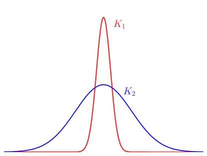
Figure 1: Schematic picture of overlapping fluctuations. Both curvatures $K_{1}$ and $K_{2}$ are centrally peaked at the same location, but can have different strength and length-scale (in the figure, $K_{2}$ represents a curvature with a larger scale compared with the one of $K_{1}$).

2 Basic set-up

We consider the approximation in which the Universe is filled by a perfect fluid with the equation of state $p=w\rho$, with constant $w$ (from now we will consider radiation fluid $w=1/3$), yielding the energy-momentum tensor

$$T^{\mu\nu}=(p+\rho)u^{\mu}u^{\nu}+pg^{\mu\nu}.$$ (2.1)

Here, $p$ is the pressure, $\rho$ is the energy density, $g^{\mu\nu}$ and $u^{\mu}$ are the components of the spacetime metric and of the four-velocity, respectively. Under the assumption of spherical symmetry, the spacetime metric can be written as

$$ds^{2}=-A(r,t)^{2}dt^{2}+B(r,t)^{2}dr^{2}+R(r,t)^{2}d\Omega^{2},$$ (2.2)

with $R(r,t)$ being the areal radius, $A(r,t)$ the lapse function, and $d\Omega^{2}\equiv d\theta^{2}+\sin^{2}(\theta)d\phi^{2}$ the line element of a two-sphere. The definition of the components of the four-velocity $u^{\mu}$ depends on the gauge chosen. In the comoving gauge, we have $u^{t}=1/A$ and $u^{i}=0$ for $i=r$, $\theta$, $\phi$. We use units in which $G_{N}=c=1$ (geometrised units).

Under this approach, we solve numerically Misner-Sharp equations following [20, 22] (see the references for details and the appendix A). The initial conditions are implemented following the gradient expansion approach [39, 40] when the cosmological fluctuations lie at much larger scales than the cosmological horizon. Then, the spacetime metric at super-horizon scales is defined as

$$ds^{2}=-dt^{2}+a^{2}(t)\mspace{-1.5mu}\left[\frac{dr^{2}}{1-K(r)r^{2}}+r^{2}d\Omega^{2}\right].$$ (2.3)

The initial conditions to solve numerically Misner-Sharp equations are given following [41, 42, 18] at the first order in gradient expansion, considering that the curvature fluctuations are initially frozen at super-horizon scales (see the appendix A for details). A well known useful strength estimator to characterise the formation of a PBH is the compaction function $\mathcal{C}$, introduced in [13]. It is defined as twice the mass excess inside a given areal radius $R$,

$$\mathcal{C}\coloneqq 2\frac{M_{\rm MS}-M_{b}}{R},$$ (2.4)

where $M_{\mathrm{MS}}\equiv 4\pi\int_{0}^{R}\rho\tilde{R}^{2}\differential{\tilde{R}}$ is the Misner–Sharp mass (which takes into account the kinetic and potential energy) and $M_{b}$ is the mass expected in the FLRW background, defined as $M_{b}=4\pi\rho_{b}R^{3}/3$. $\rho$ is the energy density of the fluid, while $\rho_{b}$ is that of the FLRW background, which evolves as $\rho_{b}=\rho_{b,0}(t/t_{0})^{-2}$. As already noticed from time ago by Shibata $\&$ Sasaki [13] and explored further in [18, 24, 1, 22, 25, 35], the compaction function’s peak is a useful estimator to characterise fluctuations that will lead to black hole formation. The criteria we follow is that if the initial compaction function contains a peak $\mathcal{C}(r_{m})$ (being $r_{m}$ the location of that peak) bigger than a given threshold, then the gravity pull will be stronger than the pressure gradients, and lead to collapsing and forming a black hole. On the opposite side, the fluctuations will be dispersed on the FLRW background. Hereafter the critical values and profiles of the compaction function will be indicated by the subscript $c$, so that the compaction function with the amplitude of the threshold value is expressed as $\mathcal{C}_{c}(r)$.

Therefore, we will characterise the amplitude of the fluctuations as the peak value of the compaction function. Specifically, at super-horizon scales, the compaction function is a time-independent quantity, whose expression in the comoving gauge was found in [18] (see their Eqs. (6.34) and (6.35)):

$$\mathcal{C}=\frac{2}{3}K(r)r^{2},$$ (2.5)

where the factor $2/3$ comes from the fact that $w=1/3$.

It was found in [1] that the averaged critical compaction function defined as

$$\bar{\mathcal{C}}_{c}\equiv\frac{3}{r_{m}^{3}}\int_{0}^{r_{m}}\mathcal{C}_{c}(\tilde{r})\tilde{r}^{2}d\tilde{r}\ ,$$ (2.6)

is approximately equal to $\bar{\mathcal{C}_{c}}=2/5$ in radiation dominated-Universe (for a generalisation with other equations of state see [22]) and mostly universal, independent of the curvature profile considered within a deviation $\mathcal{O}(2\%)$.

Another way to characterise the critical compaction function is to use the $p$ parameter (introduced in [1] ) computed as:

$$p=-\frac{\mathcal{C}^{\prime\prime}(r_{m})r^{2}_{m}}{4\mathcal{C}(r_{m})}.$$ (2.7)

Larger values of $p$ correspond to sharp profiles around the compaction function peak, and give the larger thresholds (being $2/3$ the maximum). On the other hand, small $p$ corresponds to a broad shape of $\mathcal{C}$, which gives the smaller threshold (being $0.4$ the minimum). As found in [1] different profiles/initial conditions characterised by the same $p$ lead to the same threshold value up to a deviation of $\mathcal{O}(2\%)$, which means that the threshold of the gravitational collapse mainly depends on the shape around the compaction function peaks.

Let us introduce the following specific profile of the compaction function $\mathcal{C}_{0}$ characterised by the parameter $p_{0}$ and $r_{0}$:

$$\mathcal{C}_{0}(r,\delta,p_{0},r_{0})=\delta\left(\frac{r}{r_{0}}\right)^{2}e^{\frac{1}{p_{0}}\left[1-\left(\frac{r}{r_{0}}\right)^{2p_{0}}\right]},$$ (2.8)

where the parameters $p_{0}$ and $r_{0}$ are equal to $p$ and $r_{m}$ in this profile, respectively.. The use of this profile and the value $\bar{\mathcal{C}_{c}}=2/5$ allow us to build an analytical formula given by:

$$\delta_{c}(p)=\frac{4}{15}e^{-\frac{1}{p}}\frac{p^{1-\frac{5}{2p}}}{\Gamma\left(\frac{5}{2p}\right)-\Gamma\left(\frac{5}{2p},\frac{1}{p}\right)}.$$ (2.9)

Although this formula is derived through the specific profile of the compaction function, since the same $p$ leads to the approximately same threshold value independent of the specific profile, this formula is expected to apply to any profile of the inhomogeneity.

Let’s now consider the situation where we have two overlapped compaction functions. We introduce fluctuations that are overlapped to another one on much larger scales. We therefore define two fluctuations $K_{1}$ and $K_{2}$. The “total” compaction function $\mathcal{C}$ is defined as,

$$\mathcal{C}(r)=\mathcal{C}_{1}(r,\delta_{1},p_{1},r_{1})+\mathcal{C}_{2}(r,\delta_{2},p_{2},r_{2}),$$ (2.10)

where $\mathcal{C}_{i}(r,\delta_{i},p_{i},r_{i})=\mathcal{C}_{0}(r,\delta_{i},p_{i},r_{i})$ for $i=1$ and $2$.

We define $r_{m,j}$ as the location of the peaks ($j=1,2$) of the total compaction $\mathcal{C}(r)$ and $\beta\equiv r_{m,2}/r_{m,1}$ its ratio. Notice that $r_{m,j}\approx r_{j}$, but not equal since there will be an overlap between the two curvature profiles $K_{j}$. Indeed, if we only consider one single curvature fluctuation given by $K=K_{j}:=3\mathcal{C}_{j}/(2r^{2})$ then $r_{m,j}=r_{j}$. Eqs.(2.9) is then generalised by using the effective $q_{j}$ that takes into account the $r_{m,j}$ and the total shape of the compaction function,

$$q_{j}=-\frac{\mathcal{C}^{\prime\prime}(r_{m,j})r^{2}_{m,j}}{4\mathcal{C}(r_{m,j})}.$$ (2.11)

Then the amplitude of each peak will be given by $\mathcal{C}(r_{m,1})$ and $\mathcal{C}(r_{m,2})$. Some examples of the profiles considered for different parameters can be found in Fig. 2.

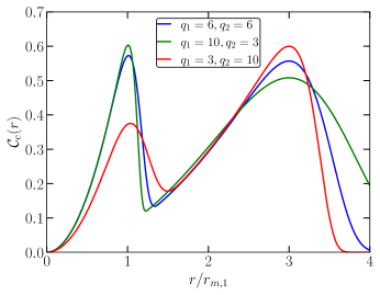
Figure 2: Examples of critical compaction function (top-left), critical curvature (top-right) and critical density contrast (bottom) for three different configurations of $q_{j}$ with $\beta=3$. The values for the density contrast and the curvature have been normalised to the peak value ($r=0$).

To quantify the degree of overlapping between the compaction functions $\mathcal{C}_{1}$ and $\mathcal{C}_{2}$, we define the following parameter

$$\xi=\frac{r_{2}-\sigma_{2}}{r_{1}+\sigma_{1}},$$ (2.12)

where we define $\sigma_{j}$ associated to each curvature $K_{j}$ as:

$$\sigma_{j}=\frac{\sqrt{\int_{0}^{\infty}\mathcal{C}_{j}(r)(r_{j}-r)^{2}dr}}{\sqrt{\int_{0}^{\infty}\mathcal{C}_{j}(r)dr}}.$$ (2.13)

The integrals can be done analytically introducing Eq.(2.8), and we obtain:

$$\sigma^{2}_{j}=\frac{3}{2}r^{2}_{j}\frac{\Gamma(3/2p_{j})-2p^{1/2p_{j}}_{j}\Gamma(2/p_{j})+p^{1/p_{j}}_{j}\Gamma(5/2p_{j})}{p_{j}\Gamma(1+3/2p_{j})}.$$ (2.14)

In Fig. 3 we show the variation of the parameter $\xi$ for different configurations of $p_{1}=p_{2}=p$ and $\beta$. When $\xi>1$ the two compaction functions $\mathcal{C}_{1}$, $\mathcal{C}_{2}$ are decoupled, in the opposite case when $\xi\rightarrow 0$ are completely coupled. $\xi$ saturates for sufficiently large values of $p_{j}$ and $\beta$. Notice that this is consistent with having completely overlapped profiles when $p_{j}\rightarrow 0$ since the compaction function becomes constant and homogeneous. It already indicates to us that for $\beta\approx 3$ with $p_{j}>3$ the initial configuration of overlapped fluctuations can be approximately considered as isolated. That is, for sufficiently small $q_{j}$ and/or $\beta$, the fluctuations are completely overlapped, and two peaks in the compaction function can not be differentiated (only a single peak). Since we are interested in the distinct overlapping fluctuations of two different scales, we restrict ourselves to the situation in which two scales are isolated with the parameters $q_{i}\geq 3$ and $\beta\geq 2$ hereafter.

Figure 3: Values of $\xi$ from Eq.(2.12) for the different configurations $p_{1}=p_{2}=p$.

We may define now the time $t_{H,j}$ that the length-scale $r_{m,j}$ takes to reenter the cosmological horizon given by

$$t_{H,j}=t_{0}\left(a_{0}\frac{r_{m,j}}{R_{H}(t_{0})}\right)^{2},$$ (2.15)

where $a_{0}$, and $t_{0}$ are gauge quantities that we set to one. Moreover, we define the mass of the cosmological horizon $M_{H}=1/(2H)$, which at the time $t_{H,j}$ is given by $M_{H}(t_{H,j})=t_{H,j}$ and $R_{H}(t_{0})=1/H_{0}$.

3 Threshold values

To explore the effect of the overlapped fluctuation on the necessary initial condition for PBH formation, we run a numerical bisection over different trial values $\delta_{1}$, $\delta_{2}$ fixing $q_{1}$, $q_{2}$ and the ratio between the length-scales $\beta\equiv r_{m,2}/r_{m,1}$ to find the critical value of the two peaks, i.e, $\mathcal{C}_{c}(r_{m,1})$ and $\mathcal{C}_{c}(r_{m,2})$ . Notice that due to the overlapping between the fluctuations, we have to tune the parameter $p_{i}$ so that a fixed value of $q_{j}$ will be realised for each numerical iteration.

With such values, we can compare the numerical thresholds from the simulations with the case of having an isolated curvature fluctuation with $p_{j}=q_{j}$ and $\mathcal{C}_{\rm c,j}(r_{j})\equiv\delta_{c,j}$. This corresponds to the peak value for the critical compaction function when we only consider a single curvature fluctuation $K_{j}$ (isolated fluctuation) and is computed following Eq.(2.9) with the effective $q_{j}$ associated to $\mathcal{C}_{c}(r_{m,j})$. We make this comparison by computing the following relative deviation,

$$\Delta\mathcal{C}_{c,j}(\%)=10^{2}\cdot\frac{\mathcal{C}_{c}(r_{m,j})-\delta_{c,j}}{\mathcal{C}_{c}(r_{m,j})}.$$ (3.1)

We have also computed the averaged critical compaction function $\bar{\mathcal{C}}_{c,j}$ integrated up to the first ($j=1$) and second peak ($j=2$), which is shown in Fig. 4. To compare with the value found in the case of having isolated fluctuations $\bar{\mathcal{C}_{c}}=2/5$ we define

$$\Delta\bar{\mathcal{C}}_{c,j}(\%)=10^{2}\cdot\frac{\bar{\mathcal{C}}_{c,j}-2/5}{2/5}.$$ (3.2)

First, let us check the relative deviation of the averaged compaction function $\bar{\mathcal{C}}$. When the gravitational collapse is lead by the first peak of the compaction function (having $\mathcal{C}_{c}(r_{m,2})$ well under threshold), the value of $\bar{\mathcal{C}}$ up to the first peak is well approximated by the value $2/5$. This starts to differ when the second peak is near the threshold value, which makes the gravitational collapse overlapped between the two fluctuations being $\bar{\mathcal{C}}_{c}$ larger than expected. The same behaviour is shown in the right panel of Fig. 4 but now considering the second peak. Although the differences between the profiles considered are not substantial, we can identify in the right panel that the deviation $\Delta\bar{\mathcal{C}}_{c,2}$ becomes larger when $q_{1}=3$ in comparison with other cases of $q_{1}$, since the compaction function profile is broader. We also note that the right and left panels in Fig. 4 are qualitatively different. More specifically, we find $\Delta\bar{\mathcal{C}}_{c,1}>0$ and $\Delta\bar{\mathcal{C}}_{c,2}<0$ in those relevant regions. Moreover, in the right panel, we can find a qualitative difference in the behaviour of $\Delta\bar{\mathcal{C}}_{c,2}$ depending on the parameter $q_{1}$. These facts indicate that the averaged critical compaction function $\bar{\mathcal{C}}_{c}$ could become sensitive to the structure inside the radius $r_{m}$ for some specific curvature profiles. Although the values of $\Delta\bar{\mathcal{C}}_{c,i}$ are not significantly large in our settings, this sensitivity may spoil the criterion with $\bar{\mathcal{C}}$ as was already observed in [43].

Figure 4: Relative deviation of the averaged critical compaction function Eq.(3.2), computed for the first peak (left-panel), and up to the second peak (right-panel). The dashed magenta lines corresponds to a deviation of $\pm 5\%$.

Next, let us check the value of $\Delta\mathcal{C}_{c,j}$. In Fig. 5, we show the numerical results for the thresholds values $\mathcal{C}_{c}(r_{m,j})$ and its relative deviation following Eq.(3.1), choosing different configurations of $q_{j}$ fixing the ratio $\beta=2$. In the top panel, the thresholds $\mathcal{C}_{c}(r_{m,j})$ are shown compared with $\Delta\mathcal{C}_{c,j}$. When $\Delta\mathcal{C}_{c,1}\ll 0$ the first peak is well under the threshold $\delta_{c,1}$ and therefore, the critical threshold value of the secondary peak is mainly given by $\mathcal{C}_{c}(r_{m,2})\rightarrow\delta_{c,2}$ (see the vertical lines in the top panels). In this case, the second peak will lead the gravitational collapse. The analogous behaviour is found when $\Delta\mathcal{C}_{c,2}\ll 0$, the second peak is well under the threshold $\delta_{c,2}$ and therefore, the critical value of the first peak is given by $\mathcal{C}_{c}(r_{m,1})\rightarrow\delta_{c,1}$, which will lead the gravitational collapse.

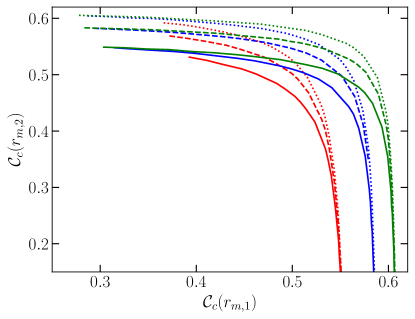
Figure 5: Top panels: Eq.(3.1) computed for the first peak and compared with the second peak (left panel) and for the vice versa (right panel) . Bottom-left panel: Phase diagram of the two thresholds ($\mathcal{C}_{c}(r_{m,1})$ , $\mathcal{C}_{c}(r_{m,2})$). Bottom-right panel: Relative deviation of Eq.(3.1) compared between both peaks.

Possibly, the most interesting case is when the two peaks are under the thresholds $\delta_{c,j}$, in other words, $\mathcal{C}_{c}(r_{m,1})<\delta_{c,1}$ and $\mathcal{C}_{c}(r_{m,2})<\delta_{c,2}$. In this case, the overlapped fluctuation will contribute to the gravitational collapse of the shorter fluctuation $K_{1}$, lowering the threshold values by a few percentages compared with the ideal case of isolated fluctuations (see bottom panels). Notice that it depends on the profile considered. For large $q_{j}$, the shape around the compaction function peak will be sharper with a small mass excess, and therefore, the overlapping between the two peaks will be smaller (compare the green lines with the red ones). Finally, the phase diagram of $\mathcal{C}_{c}(r_{m,1})$ and $\mathcal{C}_{c}(r_{m,2})$ is shown in the bottom-left panel. We find $\mathcal{C}_{c}(r_{m,2})\ll\delta_{c,2}\Rightarrow\mathcal{C}_{c}(r_{m,1})\rightarrow\delta_{c,1}$ and $\mathcal{C}_{c}(r_{m,1})\ll\delta_{c,1}\Rightarrow\mathcal{C}_{c}(r_{m,2})\rightarrow\delta_{c,2}$.

Notice that the approach of using the analytical formula $\delta_{c}(q)$ seems to be more robust in comparison with the averaged $\mathcal{C}_{c}$ when comparing the numerical results with the analytical approaches. More specifically, we do not find any qualitative difference between the behaviours of $\Delta\mathcal{C}_{c,1}$ and $\Delta\mathcal{C}_{c,2}$ unlike those in the case of the averaged compaction function.

In Fig. 6, we show the dependence of the previous quantities in terms of the distance $\beta$. For simplicity, we now consider the cases where $q_{1}=q_{2}$. Both fluctuations become more decoupled when increasing $\beta$, making the gravitational collapse dominated by one of the two peaks. This makes the relative deviations smaller when increasing $\beta$, in comparison with Figs. 4 and 5.

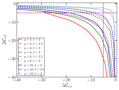
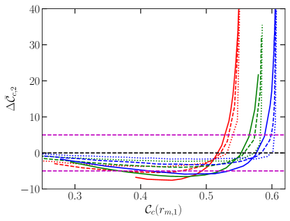
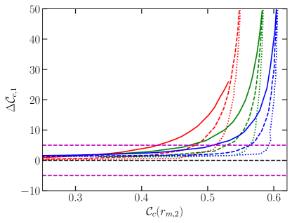
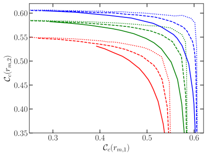
Figure 6: Top-left panel: Relative deviation of Eq.(3.1) compared between both peaks. Top-right panel: Relative deviation of the averaged critical compaction function Eq.(3.2) for the second peak. Bottom-left panel: the same as in the previous case but for the first peak. Bottom-right panel: Threshold values of the two peaks.

To quantify the extent of the effect of the overlap between the two fluctuations, we use the maximum distance between the origin and the curves of $\Delta\mathcal{C}_{c,j}$ (see the top-left panel of Fig. 6). Then, as shown in Fig. 7, the maximum deviation is around $10\%$ at worst in our settings. The deviation almost linearly depends on the parameter $\beta$ and reduces to smaller values than $5\%$ for $\beta\gtrsim 3$ depending on the parameter $q$. As expected, when the fluctuations are sufficiently separated, the threshold is well approximated by the analytic formula for each isolated peak. Our results show that even in the presence of secondary peaks, if those peaks are sufficiently separated and decoupled, the threshold of the gravitational collapse basically depends on the shape around the critical compaction function as found in [1], irrespectively of the new scale introduced.

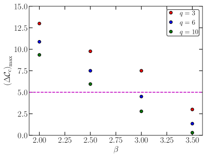
Figure 7: Maximum relative deviation Eq.(3.1) in terms of $\beta$ for different profiles.

4 Dynamical evolution and PBH mass

4.1 Dynamics of fluctuations

In this section, we study the dynamical evolution of the fluctuations in terms of the different parameters of Eq.(2.10). In Fig. 8, we show the evolution of the compaction function at some specific times, for which we can differentiate three situations. In the top-left panel we show a case where the first peak of $\mathcal{C}$ triggers the gravitational collapse when the first peak is over-threshold $\mathcal{C}(r_{m,1})>\delta_{c,1}$ being the second one $\mathcal{C}(r_{m,2})<\delta_{c,2}$. In the top-right panel instead, we show a case where the second peak triggers the gravitational collapse with $\mathcal{C}(r_{m,2})>\delta_{c,2}$ being the first one under threshold $\mathcal{C}(r_{m,1})<\delta_{c,1}$. Notice that the time needed for the growth of the fluctuation is much larger than the case $\mathcal{C}(r_{m,2})<\delta_{c,2}$ since the size of the overlapped fluctuation is much larger. In the previous cases, the peak under the threshold $\delta_{c,j}$ becomes smoothed and the mass excess disperses on the FLRW background. A different situation is found in the bottom panel, where both peaks are lower than $\mathcal{C}(r_{m,j})<\delta_{c,j}$. In this case, the two peaks will merge and collapse even when $\mathcal{C}(r_{m,j})<\delta_{c,j}$ surpassing the pressure gradients. Notice that the time scale is similar to the previous case since the contribution from the larger scale fluctuation is necessary for the collapse and the time scale is dictated by the larger scale.

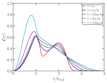
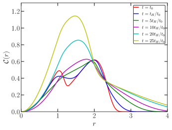
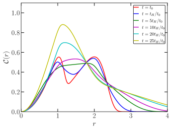
Figure 8: Snapshots of the evolution of the compaction function. Top-left panel: Case with $\delta_{1}=0.475$ and $\delta_{2}=0.5$, yielding to $\mathcal{C}(r_{m,1})=0.626$, $\mathcal{C}(r_{m,2})=0.501$. Top-right panel: $\delta_{1}=0.3$ and $\delta_{2}=0.62$, yielding to $\mathcal{C}(r_{m,1})=0.491$, $\mathcal{C}(r_{m,2})=0.620$. Bottom panel: $\delta_{1}=0.385$ and $\delta_{2}=0.555$, yielding to $\mathcal{C}(r_{m,1})=0.554$, $\mathcal{C}(r_{m,2})=0.555$. In all cases, $q_{j}=6$ with $\delta_{c,j}=0.592$ for $j=1,2$, $t_{H}$ is the time of horizon crossing when the length-scale $r_{m,1}$ reenters the cosmological horizon and $\beta=2$.

4.2 Apparent horizon formation

If an initial perturbation at super-horizon scales has a peak value of $\mathcal{C}$ bigger than its threshold, the perturbation will continue growing, and, at some point, a trapped surface will be formed. To identify when trapped surfaces are formed, we have to consider the expansion $\Theta^{\pm}$ of null geodesic congruences generated by the null vector fields $k^{\pm}$, orthogonal to a spherical surface $\Sigma$. The expansion $\Theta^{\pm}$ is defined as $\Theta^{\pm}\equiv h^{\mu\nu}\nabla_{\mu}k_{\nu}^{\pm}$, where $h^{\mu\nu}$ is the spacetime metric induced on $\Sigma$. There are two congruences: we call them inwards $k_{\mu}^{+}$ and outwards $k_{\mu}^{-}$, whose components are $k_{\mu}^{\pm}=(A,\pm B,0,0)$ with $k^{+}\cdot k^{-}=-2$.

If $\Theta^{\pm}<0$, the surface is called trapped, while if both are positive $\Theta^{\pm}>0$, the surface is anti-trapped. On the other hand, in the case of flat spacetime, $\Theta^{-}<0$ and $\Theta^{+}>0$, and these surfaces $\Sigma$ are called normal surfaces.

In our case, we have that,

$$\Theta^{\pm}=\frac{2}{R}(U\pm\Gamma),$$ (4.1)

where $U$ is the Eulerian velocity defined as $U=\dot{R}/A$ (the dot represents time derivative $\partial/\partial t$) and $\Gamma$ is given by $\Gamma=\sqrt{1+U^{2}-2M/R}$. In spherical symmetry, we can consider that any point $(r,t)$ is a closed surface $\Sigma$ with an areal radius $R$. These points can be classified as trapped, anti-trapped and normal. Specifically, the transition from a normal to a trapped surface should satisfy $\Theta^{+}=0$ and $\Theta^{-}<0$, which corresponds to a marginally trapped surface, commonly called the “apparent horizon” (AH). Taking into account that $\Theta^{+}\Theta^{-}=\frac{4}{R^{2}}(U^{2}-\Gamma^{2})$, the condition for the apparent horizon is given by $U^{2}=\Gamma^{2}\Rightarrow 2M=R$.

To have a better understanding of how the overlapped fluctuation affects the dynamical evolution of the fluctuation until the formation of the apparent horizon, we have computed the time $t_{AH}$, the location of the apparent horizon at $t_{AH}$ namely $r_{AH}$, and the PBH mass at that time $M_{\rm PBH}(t_{AH})$. Our results, done for the different three profiles: i) $q_{1}=q_{2}=6$ and $\beta=2$, ii) $q_{1}=q_{2}=6$ and $\beta=3$ and iii) $q_{1}=q_{2}=10$ and $\beta=2$, are shown in Figs. 9, 10 and 11 in log-scale and with a colour mapping.

As shown in [26], in the case of an isolated fluctuation, for strong perturbations (whose amplitude is much higher than the threshold), the time of collapse is shorter, and the PBH mass is larger compared with the case of weak fluctuations (whose amplitude is close to the threshold). This behaviour is also observed in the case of having an overlapped fluctuation. In addition to these common tendencies, they also depend on what peak is leading the gravitational collapse since the length scale of the fluctuation plays a crucial role in the PBH mass and the time to collapse. Then we can split the phase space $(\mathcal{C}(r_{m,1}),\mathcal{C}(r_{m,2}))$ for the horizon formation in the following four regions:

• Quadrant I, $\mathcal{C}(r_{m,j})>\delta_{c,j}$ for $j=1,2$: Both peaks in $\mathcal{C}(r_{m,j})$ are over-threshold, but the one with a shorter length-scale ($r_{m,1}$) will dominate the gravitational collapse before the horizon formation, independently on the value of the second peak. We also observe that increasing the amplitude of the first peak will shorten the formation time and increase the PBH mass at the time $t_{AH}$. Notice that in this case, the first apparent horizon is formed in a shorter distance than $r_{m,1}$. As we will see later on, the secondary fluctuation will play a crucial role during the accretion process from the FLRW background into the AH.

• Quadrant II, $\mathcal{C}(r_{m,1})>\delta_{c,1}$ and $\mathcal{C}(r_{m,2})<\delta_{c,2}$: Similar to the previous case, the first peak will lead the gravitational collapse whereas the second peak (under threshold) will not have a significant role for the quantities under study at $t_{AH}$.

• Quadrant III, $\mathcal{C}(r_{m,1})<\delta_{c,1}$ and $\mathcal{C}(r_{m,2})>\delta_{c,2}$: In contrast with the previous cases, now the first peak is under-threshold, and the second one will lead the gravitational collapse. Looking at the colour map, the transition from quadrant III to quadrant I is clear. But can be noticed an effect from the first peak in the boundaries of the quadrant (this is especially clear looking $M_{\rm PBH}(t_{AH})$). The time it takes the fluctuations to undergo the gravitational collapse $t_{AH}$ is larger than when the first peak leads the collapse since the length-scale is larger, implying that the PBH mass will be larger than in quadrant II. In this case, increasing the peak amplitude of the second peak will also shorten the formation time and increase the PBH mass.

• Quadrant IV, $\mathcal{C}(r_{m,1})<\delta_{c,1}$ and $\mathcal{C}(r_{m,2})<\delta_{c,2}$: Only a small region will lead to the production of PBHs. Both peaks are under the threshold $\delta_{c,j}$, and there is competition between the two peaks; indeed, the presence of a secondary peak will help the first (or vice versa) to collapse and form the apparent horizon. Interestingly, one can find the longest formation time $t_{AH}/t_{H}$ for this region. Both peaks by themselves can not lead to black hole formation and it is needed that some mass excess from the second peak merges with the first peak to be able to collapse.

The qualitative behaviour in the three cases i) – iii) is similar, but from a quantitative point of view, it depends on the specific profile considered and the ratio $\beta$. Notice that for $\beta\gg 1$, the quadrant IV will be indeed non-existent, as can be already appreciated in Fig. 10, since the peaks will behave as isolated as already noticed in Fig. 7.

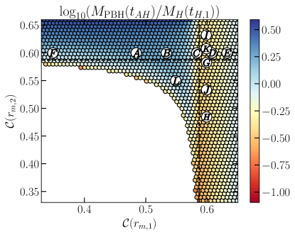
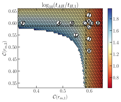
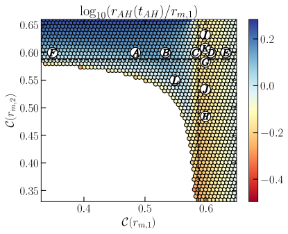
Figure 9: Top-left panel: Values of the PBH mass at $t_{AH}$ in terms of the $M_{H}(t_{H,1})$ in log scale. Top-right panel: Time that takes the fluctuation to form the apparent horizon $t_{AH}$ in terms of $t_{H,1}$ and in log scale. Bottom panel: Location of the apparent horizon at its formation $t_{AH}$ in log scale. Case for $q_{1}=q_{2}=6$ and $\beta=2$.

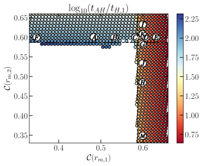
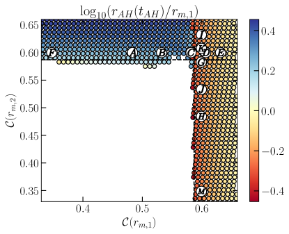
Figure 10: The same caption applies from Fig. 9, but for the case $q_{1}=q_{2}=6$ and $\beta=3$.

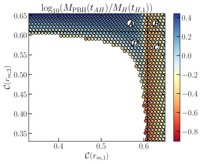
Figure 11: The same caption applies from Fig. 9, but for the case $q_{1}=q_{2}=10$ and $\beta=2$.

4.3 PBH mass after accretion

The letters in the panels of Figs. 9, 10 and 11 are the points for what we have computed the final PBH mass, that is, the mass of the PBH at the final stage after taking into account the accretion process from the surrounding FLRW background, starting from the time $t_{AH}$. To obtain the temporal evolution of the PBH mass $M_{\rm PBH}(t)$, we need to use an excision technique to remove numerically the formation of the singularity that appears soon after the formation of the apparent horizon, see [20] for details. Then, to compute $M_{\rm PBH}$ we follow the approach already used in [44, 20, 45], which consists of applying the Novikov-Zeldovich accretion formula [46] (which considers Bondi accretion [47]) once the accretion from the surrounding of the apparent horizon reaches a quasi-stationary regime, that is, the energy density just outside the apparent horizon decreases as in an FLRW universe. In practice, this is not satisfied at the time $t_{AH}$ when the assumption of a quasi-stationary flow is invalid. It is needed to wait for a sufficiently long time to obtain a quasi-stationary flow, and for that, we follow the criteria adopted in [20] such that $\dot{M}/(HM)\ll 1$.

The Novikov–Zeldovich mass accretion is given by,

$$\frac{dM_{\rm PBH}}{dt}=16\pi FM_{\rm PBH}^{2}\rho_{b},$$ (4.2)

where $F$ is a constant that corresponds to the efficiency of accretion which is commonly numerically found to be of order $\mathcal{O}(1)$ [44, 20, 45].

The integrated solution is,

$$M_{\rm PBH}(t)=\frac{1}{\frac{1}{M_{0}}+\frac{3}{2}F\quantity(\frac{1}{t}-\frac{1}{t_{0}})},$$ (4.3)

where $M_{0}$ is the PBH mass at the time $t_{0}$ when we consider the asymptotic approximation. Using the numerical evolution of the PBH mass $M_{\rm PBH}(t)$, we can make a fitting to obtain the parameters $M_{0}$ ,$t_{0}$ and $F$, and obtain the final PBH mass in the limit $M_{\rm PBH}=M_{\rm PBH}(t\longrightarrow\infty)$, when the increase in time of the mass will be very small. We find the values of $F$ to be $F\approx 3.5$, consistent with what was found in [20]. A plot of the evolution of the PBH mass for some of the points located in Figs. 9, 10 and 11 is shown in Fig. 12.

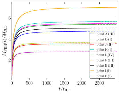
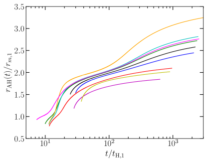
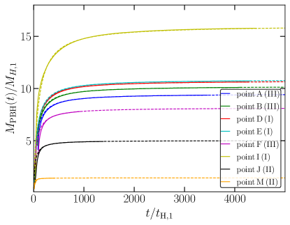
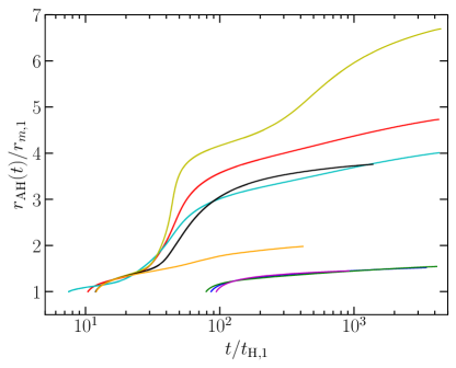
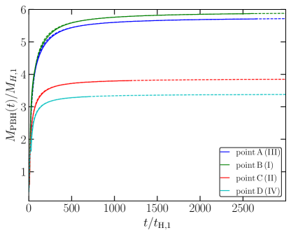
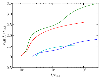
Figure 12: Left-column: Time-evolution of the PBH mass for different initial conditions (solid-line) compared with the analytical fit of Eq.(4.3) (dashed-line). Right-column: Evolution of the location of the apparent horizon in time for different configuration. Top-panels: Cases from Fig. 9. Middle-panels: Cases from Fig. 10. Bottom panel: Cases from Fig. 11. The symbols I,II,III,IV in parentheses indicates the quadrant where the points are located.

Let’s focus on the first row of Fig. 12. The initial PBH mass at the time $t_{AH}$ increases substantially thanks to the accretion of the FLRW background. The dashed line corresponds to the analytical formula of Eq.(4.3), which fits very well the numerical $M_{\rm PBH}(t)$ for late times. The location of the apparent horizon in time is shown in the right panel. For the points A,B,F,L, the second peak leads the gravitational collapse, whereas for the points D,E,J,K, the first peak dominates the collapse before the horizon formation. When the first peak of $\mathcal{C}$ leads the gravitational collapse, the apparent horizon will soon interact and absorb the mass excess of the second peak, which leads to a step-like increase of the radial coordinate $r_{\rm AH}$ as can be appreciated. This differs from the points A,B,F,L since at the formation of the AH already the mass excess from the first peak lies within $r_{AH}$, and the accretion process that follows accounts only for the tail of the secondary peak and the FLRW background. To understand the quantitative effects of the overlapping fluctuations on the PBH mass, we should refer to the data shown in Table 1.

The final mass of the PBH depends on the amplitude of each peak and what peak will lead to the collapse. For instance, if we compare the points I and E, both have very similar peak values when exchanged, but the mass is larger in the case of I since the secondary peak, which has a larger length scale, has a higher amplitude and dominates the gravitational collapse.

Even when the second peak triggers the gravitational collapse, the mass excess from the first peak also contributes to the PBH mass since the AH encloses that. For instance, for the point C, the final PBH mass $\approx 5.34M_{H}(t_{H,1})$ is larger than the respective sums of having isolated fluctuations (the last two rows in 1) which would be $\approx 4.13M_{H}(t_{H,1})$. In this case, the mass excess of the first peak doesn’t lose its mass because of pressure gradients, compared to having the first peak isolated. Notice that for the case I (I quadrant), we have the case with the largest PBH mass since it has the largest $\mathcal{C}(r_{m,2})$ in comparison with other cases.

In the table, we also show the ratio $M_{\rm PBH}/M_{\rm PBH}(t_{AH})$, which gives an idea of the increase of the PBH from the time $t_{AH}$. When the second peak leads the gravitational collapse, the accretion increases the PBH mass by a factor $\sim 2$ (as in the case of an isolated fluctuation), since the dynamical behaviour will be similar to having an isolated fluctuation: only capturing the tail of the mass excess of the fluctuation that produces the apparent horizon. The situation is different when the first peak leads to collapse since it can capture all the mass excess from the secondary fluctuation, as discussed before, making this ratio much larger.

In the second row in Fig. 12, we have the case with the same $q_{1}=q_{2}=6$ but with a larger separation between the peaks $\beta=3$ instead of $\beta=2$ (see Table 2). The qualitative behaviour is similar, but notice that since the second peak lies on much larger scales, the accretion from the FLRW background is larger when the first peaks first form the AH, whereas the ratio $M_{\rm PBH}/M_{\rm PBH}(t_{AH})$ remains as a factor $\sim 2$ when the second peak leads the collapse.

In the last row in Fig. 12, we have shown the case $q_{1}=q_{2}=10$ with $\beta=2$ (see Table 3). The qualitative behaviour is similar to the case of the first row. However, we find differences in the PBH mass (in particular smaller in some cases) with smaller mass excess for large $q$ (comparing with equal peak amplitude $\mathcal{C}$) as noticed in [26]. It is due to large pressure gradients that reduce the effect of accretion.

$\mathcal{C}(r_{m,1})$	$\mathcal{C}(r_{m,2})$	$M_{\rm PBH}/M_{H}(t_{H,1})$	$M_{\rm PBH}/M_{\rm PBH}(t_{AH})$	Point
0.608	0.600	5.45	8.36	D (I)
0.632	0.600	5.53	6.27	E (I)
0.599	0.632	7.09	10.92	I (I)
0.599	0.608	5.72	9.25	K (I)
0.599	0.583	4.80	8.09	G (II)
0.599	0.484	2.82	5.50	H (II)
0.599	0.533	3.59	6.53	J (II)
0.484	0.600	4.79	2.14	A (III)
0.534	0.600	5.10	2.34	B (III)
0.583	0.600	5.34	6.09	C (III)
0.349	0.600	3.70	2.28	F (III)
0.549	0.550	2.81	1.98	L (IV)
0.599	0.0	0.78	2.17	/
0.0	0.600	3.35	2.21	/

Table 1: Table of data for the final PBH mass estimated following Eq.(4.3) and corresponding to the case of Fig. 9 for $\beta=2$ and $q_{1}=q_{2}=6$. The last two arrows correspond to the case of having isolated peaks, i.e, without having overlapped fluctuations. The symbols inside the parenthesis specify the quadrant. Notice that the numerical results are given up to some significant digits.

$\mathcal{C}(r_{m,1})$	$\mathcal{C}(r_{m,2})$	$M_{\rm PBH}/M_{H}(t_{H,1})$	$M_{\rm PBH}/M_{\rm PBH}(t_{AH})$	Point
0.607	0.600	10.77	21.36	D (I)
0.632	0.600	10.88	13.54	E (I)
0.599	0.632	16.07	14.40	I (I)
0.599	0.608	11.77	27.56	K (I)
0.599	0.583	8.76	20.83	G (II)
0.599	0.484	3.11	7.56	H (II)
0.599	0.533	5.02	12.02	J (II)
0.599	0.349	1.44	3.67	M (II)
0.484	0.600	9.50	2.29	A (III)
0.532	0.600	10.24	2.25	B (III)
0.582	0.600	10.63	2.81	C (III)
0.348	0.600	8.17	2.25	F (III)

Table 2: Table of data for the final PBH mass estimated following Eq.(4.3) and corresponding to the case of Fig. 10 for $\beta=3$ and $q_{1}=q_{2}=6$. The symbols inside the parenthesis specify the quadrant.

$\mathcal{C}(r_{m,1})$	$\mathcal{C}(r_{m,2})$	$M_{\rm PBH}/M_{H}(t_{H,1})$	$M_{\rm PBH}/M_{\rm PBH}(t_{AH})$	Point
0.629	0.630	5.94	9.36	B (I)
0.629	0.570	3.87	6.32	C (II)
0.569	0.630	5.77	2.45	A (III)
0.579	0.580	3.40	2.08	D (IV)

Table 3: Table of data for the final PBH mass estimated following Eq.(4.3) and corresponding to the case of Fig. 11 for $\beta=2$ and $q_{1}=q_{2}=10$. The symbols inside the parenthesis specify the quadrant.

4.4 Double trapped surface

In the previous section, we have focused on the case when the fluctuations are not so separated, with $\beta$ being $\mathcal{O}(1)$. We now consider the case when the fluctuations are highly isolated ($\beta\gg 1$) and both peaks of $\mathcal{C}$ are over-threshold. Suppose the amplitude of both peaks is over-threshold, and both fluctuations are sufficiently separated. In that case, we will form for sufficiently late time two-trapped surfaces, in contrast with a single AH as shown in the previous cases of Fig. 12 (see also [48]).

Specifically, first the apparent horizon corresponding to the shorter fluctuation $\mathcal{C}_{1}$ is formed. Then, if the second peak of $\mathcal{C}$ is sufficiently separated from the first one, the AH will not be able to swallow that mass excess, allowing it to form another AH without a substantial interaction with the first one. In this case, a new trapped surface is formed, which is separated from the previous one by a normal region $\Theta^{+}>0$ and $\Theta^{-}<0$. An example can be found in Fig. 13.

First, let’s focus on a case similar to the previous ones in Fig. 12 with $q_{1}=q_{2}=6$ and $\beta=7$. The green lines correspond to a case with $\beta=7$, where it is clear that the AH (solid line) from the beginning captures the mass excess from the overlapped fluctuation $\mathcal{C}_{2}$, largely increasing its coordinate radius (see left-panels of Fig. 14). In this case, there is only one connected trapped region surrounded by the marginally trapped surface (apparent horizon) separating the trapped region from the outer normal region. The normal region is also bounded by the marginally anti-trapped surface (cosmological horizon) separating the normal region from the anti-trapped region (see right-panels of Fig. 14).

The situation differs for the case $\beta=15$, for what at $t/t_{H,1}\approx 10^{3}$, a new trapped region emerges (between the magenta and cyan lines in Fig. 13) that surrounds the already existing one (red line). Specifically, checking the expansion of the congruences $\Theta^{\pm}$ from Fig. 14, it is noticed that the magenta line in Fig. 13 corresponds to the new apparent horizon, whereas the cyan line to an inner horizon. Indeed, we have the same situation of the pair creation of the outer and inner horizons when the first apparent horizon is formed at $t_{AH}$ although it is hard to see due to the excision procedure. To proceed with the simulation, removing the computational domain that lies inside the new apparent horizon would be necessary. For this situation, when $\beta\gg 1$, the PBH mass is clearly dominated by the secondary fluctuation $\mathcal{C}_{2}$. This result is consistent with what was found in [48] for a specific curvature profile, where the phenomena called “double PBH formation” was noticed.

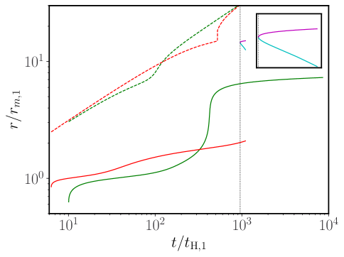
Figure 13: The solid line corresponds to the location of the AH $r_{AH}$, whereas the dashed line corresponds to the cosmological horizon. The green line corresponds to the case $\beta=7$, and red for the case with $\beta=15$ (the case which corresponds to the formation of a double trapped surface). The subplot make a zoom at the time when the second AH is formed at $t/t_{H,1}\approx 10^{3}$. The magenta line corresponds to the new AH, and the cyan line to the horizon surrounded by the normal region, which moves inwards the computational domain.

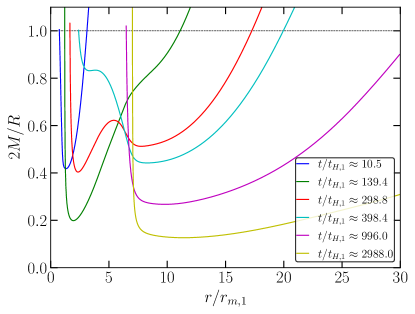
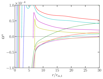
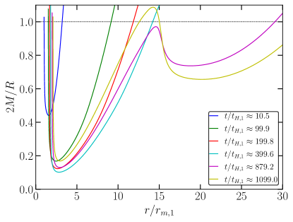
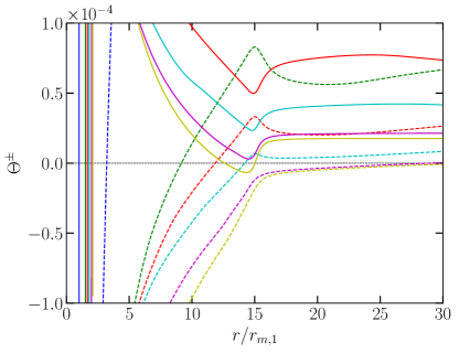
Figure 14: Top-left panel: Snapshots of the compactness $2M/R$ (solid line) at different times. Top-right panel: Snapshots of the congruences $\Theta^{+}$ (solid line) and $\Theta^{-}$ (dashed line) at different times. Bottom panels: The same as in the top panels but with the case $\beta=15$ instead of $\beta=7$, where the double trapped surface formation is shown.

The phenomena of formation of a double trapped surface formation instead of a single AH depends mainly on the separation of scales between the peaks of $\mathcal{C}$ controlled by the parameter $\beta$, but also on the specific profile and the amplitudes for both peaks. Specifically, the second peak needs to have sufficient mass excess, so that it collapses to form an apparent horizon once it reenters the cosmological horizon with the first AH not accreting a substantial amount of mass excess from the second peak before the collapse of the second peak. It should be also noted that, in general, the realisation of the double AH formation depends on the condition of time slicing. That is, we may choose a different gauge for the time slicing in which only one connected trapped region continues to exist after the horizon formation.

5 Summary and Conclusions

In this work, we have studied the PBH formation process from the collapse of overlapping curvature fluctuations. To do that, we have used numerical simulations of the gravitational collapse of the super-horizon curvature fluctuations considering the formalism of the compaction function $\mathcal{C}$ to set up the initial conditions.

Using a set of curvature profiles with different parameters, we have shown that when the length scales of two overlapped fluctuations are well separated and fluctuations are sufficiently decoupled, the threshold of PBH formation can be characterized by the shape around the compaction function’s peak that is leading to the gravitational collapse, where analytical formulas $\delta_{c}(q)$ can be accurately applied. Meanwhile, depending on the degree of overlapping between the fluctuations, the threshold can be reduced by a few percentages compared to having isolated peaks in $\mathcal{C}$. Therefore, our results confirm that the threshold for PBH formation is mainly characterized by the shape around the compaction function peak that is leading the gravitational collapse, even in the case of considering a multi-scale problem as done in this work.

Moreover, we have studied in detail the dynamics of PBH formation for different initial conditions and the effect on the PBH mass. When both peaks are sufficiently closer to each other, a single AH surrounded by the cosmological horizon is formed. When the first peak is over the threshold, the AH swallows the mass excess from the fluctuations with a larger length scale once the AH grows to such scales, and the accretion from the larger length scale fluctuation mainly gives the final PBH mass. On the other hand, when the second peak is over the threshold (having the first one under the threshold), it will lead to the gravitational collapse, capturing already all the mass excess inside the AH. The situation differs when both fluctuations are over the threshold but sufficiently decoupled. For that case, the second peak of $\mathcal{C}$ can have enough time to form a new AH without the interaction of the previous one forming a double trapped surface. In the context of the effects of profile dependence on PBH formation, we have shown that profile dependence can substantially affect the process of forming PBHs, regarding the threshold values, and importantly for the final PBH mass.

Future extensions of our work could be to generalize our calculations in the context of a general equation of state $w$ as in [22]. Another direction can be to explore the corresponding critical regime [49] and find its dependence in terms of the different initial conditions of the double peaks in $\mathcal{C}$. Finally, using peak theory, it could be interesting to make an accurate statistical prediction of the probability of having such overlapping fluctuations cases. Although the expectation is that the probability will be very small, the reduction in the threshold values could compensate for the large reduction of the PBH production formed in this scenario. All these features are interesting future research directions.

Appendix A Details of the numerical set-up

In this work, we have used the publicly available numerical code offered by [20, 50] to simulate numerically the formation of PBHs from the collapse of the curvature fluctuations on the FLRW universe filled by radiation fluid ($w=1/3$). The code uses Pseudospectral methods, and we refer the reader to [20] for more details. Specifically, we numerically solve Misner–Sharp equations [51], which describes the gravitational collapse of a perfect fluid with spherical symmetry. Solving Einstein equations taking into account Eqs.(2.1),(2.2) and assuming a constant equation of state like $p=w\rho$ we obtain,

$$\dot{U} =-A\left[\frac{w}{1+w}\frac{\Gamma^{2}}{\rho}\frac{\rho^{\prime}}{R^{\prime}}+\frac{M}{R^{2}}+4\pi Rw\rho\right],$$ (A.1)

$$\dot{R} =AU,$$

$$\dot{\rho} =-A\rho(1+w)\left(2\frac{U}{R}+\frac{U^{\prime}}{R^{\prime}}\right),$$

$$\dot{M} =-4\pi Aw\rho UR^{2},$$

where we have used $\Gamma=R^{\prime}/B$ and the lapse $A$ can be solved analytically as $A(r,t)=[\rho_{b}(t)/\rho(r,t)]^{1/4}$, which is smoothly connected to the FLRW background in $r\to\infty$. The initial condition on the set of Eqs. (A.1) is imposed on a super-Hubble scale so that it is connected to the perturbed metric (2.2), as in [41, 42, 17]. There, the gradient expansion method is applied to this end. That is, the radial dependence of the Misner–Sharp equations is expanded in the gradient parameter $\epsilon(t)$ defined by

$$\epsilon(t)\equiv\frac{1}{H(t)L(t)},$$ (A.2)

where $H(t)$ is the Hubble factor and $L(t)\coloneqq a(t)r_{m,1}$ is the length scale of the fluctuation $K_{1}$ at super-horizon scales. It results in the following initial conditions [41, 42, 17]:

$$A(r,t) =1+\epsilon^{2}(t)\tilde{A},$$

$$R(r,t) =a(t)r(1+\epsilon^{2}(t)\tilde{R}),$$

$$U(r,t) =H(t)R(r,t)(1+\epsilon^{2}(t)\tilde{U}),$$ (A.3)

$$\rho(r,t) =\rho_{b}(t)(1+\epsilon^{2}(t)\tilde{\rho}),$$

$$M(r,t) =\frac{4\pi}{3}\rho_{b}(t)R(r,t)^{3}(1+\epsilon^{2}(t)\tilde{M}),$$

where for $\epsilon\rightarrow 0$, we recover the (FLRW) solution. The perturbations for the tilde variables at $\mathcal{O}(\epsilon^{2})$ order in gradient expansion are shown in [41, 42, 17], which we summarise here:

$$\tilde{\rho} =\frac{3(1+w)}{5+3\omega}\left[K(r)+\frac{r}{3}K^{\prime}(r)\right]r^{2}_{m,1},$$

$$\tilde{U} =-\frac{1}{5+3\omega}K(r)r^{2}_{m,1},$$

$$\tilde{A} =-\frac{w}{1+w}\tilde{\rho},$$ (A.4)

$$\tilde{M} =-3(1+w)\tilde{U},$$

$$\tilde{R} =-\frac{w}{(1+3\omega)(1+w)}\tilde{\rho}+\frac{1}{1+3\omega}\tilde{U}.$$

Introducing the parameters $\delta_{1},\delta_{2},r_{1},r_{2}$ we build the initial curvature profile following Eqs.(2.5),(2.8) and for what we can find numerically $r_{m,1}$ (defined as the first peak in $\mathcal{C}$). Then, the initial condition can be set up.

We have ensured that for each initial configuration, the epsilon parameter is less than $\epsilon(t_{0})\lesssim 10^{-1}$ (this ensures that the first order in gradient expansion is enough accurate [42]), specifically we consider $\epsilon(t_{0})\sim 0.1$. Note that the choice of different gauges should give equivalent numerical results up to $\mathcal{O}(\epsilon^{2})$ as shown in [18].

The initial time of our simulations is normalised as $t_{0}=1$ and the background conditions are given at that time by $a(t_{0})=1$, $R_{H}(t_{0})\coloneqq 1/H(t_{0})=2t_{0}$, and $\rho_{b}(t_{0})=3H^{2}(t_{0})/8\pi$. We use two-three Chebyshev grids with size $N\approx 400$ (although for some cases the number of points is increased) to cover the different regions where higher resolution is needed. The boundary conditions are specified in [20]. The time step is chosen as $\differential{t}=\differential{t_{0}}(t/t_{0})^{1/2}$ with $\differential{t_{0}}\sim 10^{-3}$.

Once the apparent horizon is formed, we remove part of the computational domain (excision technique) when $\mathcal{C}_{\rm max}\approx 1.1$ (the maximum value of $\mathcal{C}$) to avoid the formation of a singularity that will appear soon after $t_{AH}$. See [20] for details of the implementation, which are very similar to our case.

Appendix B Numerical convergence

To check the reliability of our simulations, we have performed some tests of convergence for our simulations to ensure the accuracy of the results. To do that we use the Hamiltonian constrain equation $M^{\prime}\equiv 4\pi R^{\prime}R^{2}\rho$ to define the quantity,

$$\mathcal{H}\equiv\frac{M^{\prime}_{\rm num}-M^{\prime}_{\rm def}}{M^{\prime}_{\rm def}}=\frac{M^{\prime}_{\rm num}/R^{\prime}_{\rm num}}{4\pi\rho_{\rm num}R^{2}_{\rm num}}-1,$$ (B.1)

where the numerical square norm is given by,

$$\mid\mathcal{H}\mid\equiv\frac{1}{N_{\rm cheb}}\sqrt{\sum_{i=1}^{N}\left(\frac{M^{\prime}_{i}/R^{\prime}_{i}}{4\pi\rho_{i}R^{2}_{i}}-1\right)^{2}}.$$ (B.2)

The $N_{\rm cheb}$ is the total number of grid points, and the sub-index $i$ refers to each grid point. For self-consistent of the numerical simulation $\mid\mathcal{H}\mid$ should be much smaller than one. An example of the convergence of our simulations is shown in Fig. 15 for the estimation of the PBH mass in section 4 (similar behaviour is found in the accuracy on determining the thresholds values in section 3).

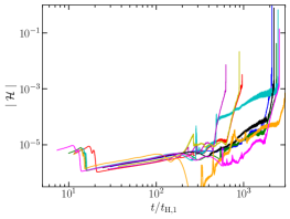
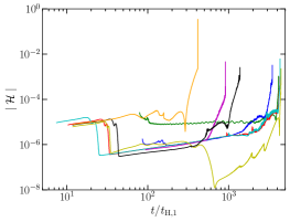
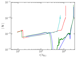
Figure 15: Numerical evolution of Eq.(B.2) for the cases $q_{1}=q_{2}=6,\beta=2$ (left-panel), $q_{1}=q_{2}=6,\beta=3$ (middle-panel) and $q_{1}=q_{2}=10,\beta=2$ (right-panel). The evolution shown in the plot starts from the time when the apparent horizon is formed. The legend for each case is the same as in Fig. 12.

The numerical fitting to the evolution of the PBH mass shown in Fig. 12 is taken in the region where the constraints are fulfilled but at sufficiently late times where the regime of applicability of Eq.(4.3) is accurate. In other words, the last part of the numerical evolution where is found a substantial increment of the Hamiltonian constraints (due to an insufficient resolution of the grid ) is not taken into account. Although that, the evolution of the PBH mass seems not to be substantially affected by that.

References

- [1] A. Escrivà, C. Germani and R.K. Sheth, Universal threshold for primordial black hole formation, Phys. Rev. D 101 (2020) 044022.
- [2] B.J. Carr and S.W. Hawking, Black holes in the early Universe, Mon. Not. Roy. Astron. Soc. 168 (1974) 399.
- [3] B.J. Carr, The Primordial black hole mass spectrum, Astrophys. J. 201 (1975) 1.
- [4] A. Escrivà, F. Kuhnel and Y. Tada, Primordial Black Holes, 2211.05767.
- [5] C.-M. Yoo, The Basics of Primordial Black Hole Formation and Abundance Estimation, Galaxies 10 (2022) 112 [2211.13512].
- [6] J.M. Overduin and P.S. Wesson, Dark matter and background light, Phys. Rept. 402 (2004) 267 [astro-ph/0407207].
- [7] P.H. Frampton, M. Kawasaki, F. Takahashi and T.T. Yanagida, Primordial Black Holes as All Dark Matter, JCAP 04 (2010) 023 [1001.2308].
- [8] S. Bird, I. Cholis, J.B. Muñoz, Y. Ali-Haïmoud, M. Kamionkowski, E.D. Kovetz et al., Did LIGO detect dark matter?, Phys. Rev. Lett. 116 (2016) 201301 [1603.00464].
- [9] B.J. Carr, K. Kohri, Y. Sendouda and J. Yokoyama, New cosmological constraints on primordial black holes, Phys. Rev. D 81 (2010) 104019 [0912.5297].
- [10] B. Carr, F. Kuhnel and M. Sandstad, Primordial Black Holes as Dark Matter, Phys. Rev. D 94 (2016) 083504 [1607.06077].
- [11] B. Carr, K. Kohri, Y. Sendouda and J. Yokoyama, Constraints on primordial black holes, Rept. Prog. Phys. 84 (2021) 116902 [2002.12778].
- [12] LIGO Scientific, Virgo collaboration, Observation of Gravitational Waves from a Binary Black Hole Merger, Phys. Rev. Lett. 116 (2016) 061102 [1602.03837].
- [13] M. Shibata and M. Sasaki, Black hole formation in the Friedmann universe: Formulation and computation in numerical relativity, Phys. Rev. D 60 (1999) 084002 [gr-qc/9905064].
- [14] J.C. Niemeyer and K. Jedamzik, Dynamics of primordial black hole formation, Phys. Rev. D 59 (1999) 124013.
- [15] I. Hawke and J.M. Stewart, The dynamics of primordial black-hole formation, Classical and Quantum Gravity 19 (2002) 3687.
- [16] I. Musco, J.C. Miller and L. Rezzolla, Computations of primordial black hole formation, Class. Quant. Grav. 22 (2005) 1405 [gr-qc/0412063].
- [17] T. Nakama, T. Harada, A.G. Polnarev and J. Yokoyama, Identifying the most crucial parameters of the initial curvature profile for primordial black hole formation, J. Cosmology Astropart. Phys 2014 (2014) 037 [1310.3007].
- [18] T. Harada, C.-M. Yoo, T. Nakama and Y. Koga, Cosmological long-wavelength solutions and primordial black hole formation, Phys. Rev. D 91 (2015) 084057.
- [19] C.T. Byrnes, M. Hindmarsh, S. Young and M.R.S. Hawkins, Primordial black holes with an accurate QCD equation of state, J. Cosmology Astropart. Phys 2018 (2018) 041 [1801.06138].
- [20] A. Escrivà, Simulation of primordial black hole formation using pseudo-spectral methods, Physics of the Dark Universe 27 (2020) 100466.
- [21] C.-M. Yoo, T. Harada and H. Okawa, Threshold of Primordial Black Hole Formation in Nonspherical Collapse, Phys. Rev. D 102 (2020) 043526 [2004.01042].
- [22] A. Escrivà, C. Germani and R.K. Sheth, Analytical thresholds for black hole formation in general cosmological backgrounds, JCAP 01 (2021) 030 [2007.05564].
- [23] T. Kokubu, K. Kyutoku, K. Kohri and T. Harada, Effect of Inhomogeneity on Primordial Black Hole Formation in the Matter Dominated Era, Phys. Rev. D 98 (2018) 123024 [1810.03490].
- [24] I. Musco, Threshold for primordial black holes: Dependence on the shape of the cosmological perturbations, Phys. Rev. D 100 (2019) 123524 [1809.02127].
- [25] I. Musco, V. De Luca, G. Franciolini and A. Riotto, Threshold for primordial black holes. II. A simple analytic prescription, Phys. Rev. D 103 (2021) 063538 [2011.03014].
- [26] A. Escrivà and A.E. Romano, Effects of the shape of curvature peaks on the size of primordial black holes, JCAP 05 (2021) 066 [2103.03867].
- [27] A. Escrivà, E. Bagui and S. Clesse, Simulations of PBH formation at the QCD epoch and comparison with the GWTC-3 catalog, JCAP 05 (2023) 004 [2209.06196].
- [28] G. Franciolini, I. Musco, P. Pani and A. Urbano, From inflation to black hole mergers and back again: Gravitational-wave data-driven constraints on inflationary scenarios with a first-principle model of primordial black holes across the QCD epoch, Phys. Rev. D 106 (2022) 123526 [2209.05959].
- [29] T. Harada, K. Kohri, M. Sasaki, T. Terada and C.-M. Yoo, Threshold of primordial black hole formation against velocity dispersion in matter-dominated era, JCAP 02 (2023) 038 [2211.13950].
- [30] A. Escrivà and J.G. Subils, Primordial Black Hole Formation during a Strongly Coupled Crossover, arXiv e-prints (2022) arXiv:2211.15674 [2211.15674].
- [31] A. Escrivà, PBH Formation from Spherically Symmetric Hydrodynamical Perturbations: A Review, Universe 8 (2022) 66 [2111.12693].
- [32] T. Harada, C.-M. Yoo and K. Kohri, Threshold of primordial black hole formation, Phys. Rev. D 88 (2013) 084051 [1309.4201].
- [33] T. Papanikolaou, Toward the primordial black hole formation threshold in a time-dependent equation-of-state background, Phys. Rev. D 105 (2022) 124055 [2205.07748].
- [34] T. Papanikolaou, Primordial black holes in loop quantum cosmology: the effect on the threshold, Class. Quant. Grav. 40 (2023) 134001 [2301.11439].
- [35] T. Harada, C.-M. Yoo and Y. Koga, Revisiting compaction functions for primordial black hole formation, Phys. Rev. D 108 (2023) 043515 [2304.13284].
- [36] V. Atal, J. Cid, A. Escrivà and J. Garriga, PBH in single field inflation: the effect of shape dispersion and non-Gaussianities, J. Cosmology Astropart. Phys 2020 (2020) 022 [1908.11357].
- [37] J.M. Bardeen, J.R. Bond, N. Kaiser and A.S. Szalay, The Statistics of Peaks of Gaussian Random Fields, ApJ 304 (1986) 15.
- [38] Y. Fukui, A. Habe, T. Inoue, R. Enokiya and K. Tachihara, Cloud–cloud collisions and triggered star formation, Publications of the Astronomical Society of Japan 73 (2020) S1 [https://academic.oup.com/pasj/article-pdf/73/Supplement_1/S1/36134093/psaa103.pdf].
- [39] Y. Nambu and A. Taruya, Application of gradient expansion to an inflationary universe, Classical and Quantum Gravity 13 (1996) 705 [astro-ph/9411013].
- [40] A. Taruya and Y. Nambu, Application of Gradient Expansion to Non-Linear Gravitational Wave in Plane-Symmetric Universe, Progress of Theoretical Physics 95 (1996) 295 [gr-qc/9510010].
- [41] A.G. Polnarev and I. Musco, Curvature profiles as initial conditions for primordial black hole formation, Class. Quant. Grav. 24 (2007) 1405 [gr-qc/0605122].
- [42] A.G. Polnarev, T. Nakama and J. Yokoyama, Self-consistent initial conditions for primordial black hole formation, J. Cosmology Astropart. Phys 2012 (2012) 027 [1204.6601].
- [43] A. Escrivà, Y. Tada, S. Yokoyama and C.-M. Yoo, Simulation of primordial black holes with large negative non-Gaussianity, J. Cosmology Astropart. Phys 2022 (2022) 012 [2202.01028].
- [44] H. Deng, J. Garriga and A. Vilenkin, Primordial black hole and wormhole formation by domain walls, JCAP 04 (2017) 050 [1612.03753].
- [45] C.-M. Yoo, T. Harada, S. Hirano, H. Okawa and M. Sasaki, Primordial black hole formation from massless scalar isocurvature, 2112.12335.
- [46] Y.B. Zel’dovich and I.D. Novikov, The Hypothesis of Cores Retarded during Expansion and the Hot Cosmological Model, Soviet Astron. AJ (Engl. Transl. ), 10 (1967) 602.
- [47] H. Bondi, On spherically symmetrical accretion, MNRAS 112 (1952) 195.
- [48] T. Nakama, The double formation of primordial black holes, JCAP 10 (2014) 040 [1408.0955].
- [49] C. Gundlach and J.M. Martin-Garcia, Critical phenomena in gravitational collapse, Living Rev. Rel. 10 (2007) 5 [0711.4620].
- [50] A. Escrivà. https://www.albertescriva.com/.
- [51] C.W. Misner and D.H. Sharp, Relativistic Equations for Adiabatic, Spherically Symmetric Gravitational Collapse, Physical Review 136 (1964) 571.