Exploring the Formation of Resistive Pseudodisks with the GPU Code Astaroth

Abstract

Pseudodisks are dense structures formed perpendicular to the direction of the magnetic field during the gravitational collapse of a molecular cloud core. Numerical simulations of the formation of pseudodisks are usually computationally expensive with conventional CPU codes. To demonstrate the proof-of-concept of a fast computing method for this numerically costly problem, we explore the GPU-powered MHD code Astaroth, a 6th-order finite difference method with low adjustable finite resistivity implemented with sink particles. The formation of pseudodisks is physically and numerically robust and can be achieved with a simple and clean setup for this newly adopted numerical approach for science verification. The method’s potential is illustrated by evidencing the dependence on the initial magnetic field strength of specific physical features accompanying the formation of pseudodisks, e.g. the occurrence of infall shocks and the variable behavior of the mass and magnetic flux accreted on the central object. As a performance test, we measure both weak and strong scaling of our implementation to find most efficient way to use the code on a multi-GPU system. Once suitable physics and problem-specific implementations are realized, the GPU-accelerated code is an efficient option for 3-D magnetized collapse problems.

1 Introduction

Pseudodisks are disklike density structures produced during the gravitational collapse of magnetized cloud cores Galli & Shu (1993a, b, hereafter GS93I,II). Observationally, they can be identified as flattened structures perpendicular to the magnetic field orientation, with infall signatures on their radial velocity profile. In the direction perpendicular to the field, the motion is hindered relative to that along the field. The Lorentz force deflects the infall motion from going radially to the protostar, producing a density enhancement perpendicular to the direction of the magnetic field lines. They are transitional, nonequilibrium structures where the gas continues its collapse to the center. Infall motions essentially dominate pseudodisks and are not rotationally supported as Keplerian disks are.

The predicted sizes of pseudodisks around young stars are on the order of several thousand au. One of the first of such observed objects was the large flattened gas envelope of HL Tau, which was observed to have infalling motions at a scale of $2000{\mathrm{\,au}}$ by Hayashi et al. (1993). This source has also recently been revealed by ALMA Partnership et al. (2015) in the inner $100{\mathrm{\,au}}$ radius, a thin dust disk with concentric rings and gaps. The inner gas disk must be rotationally supported, rather than being a pseudodisk like its large-scale gas envelope. The Atacama Large Millimeter/submillimeter Array has shown several other Class 0 sources with the characteristics of pseudodisks such as HH 211, HH 1448 IRS 2, L1157, B335, and NGC 1333 IRAS 4A (see Section 5.1).

The theoretical concept of pseudodisks is rooted in an extension of the self-similar singular isothermal sphere (SIS) collapse solution of Shu (1977) into a more realistic physical situation that includes the effect of the magnetic field. Following Terebey et al. (1984), who introduced rotation into the SIS solution using a perturbative approach, GS93I used a similar kind of perturbation analysis to account for the effects of magnetic fields. The perturbation solution of GS93I includes the impact of magnetic feedback on the gas dynamics. GS93II tested this perturbation solution numerically. GS93I and II assumed an SIS threaded by a uniform magnetic field as the initial state for simplicity. Later, Li & Shu (1996) proposed quasi-static magnetized toroids in force balance as initial states for the gravitational collapse of magnetized clouds.

Direct numerical MHD collapse simulations are computationally expensive, as they in general require high-performance computing resources to be properly executed for scientifically significant purposes. Magnetized collapse is inherently a multiscale phenomenon, needing a large scale to start the collapse and a small scale for the structures produced by the collapse (e.g., pseudodisk thickness). That requires a large computational volume to be solved during the time necessary for the collapse to occur; while that time is fortunately usually not too long, in comparison to e.g. the lifetime of protoplanetary disks, the computational time step (controlled by the Courant condition) is often dominated in MHD problems by those computational cells naturally having a locally large Alfvén speed (with a large field intensity but low $\rho$), and usually leading to a time step much smaller than the collapse time scales. The time step size may also be restricted by the need to simulate nonideal MHD and other diffusive processes.

We experiment with a new fast method with GPU technology to identify a computationally cost effecient strategy for this problem. We explore the characteristics of the pseudodisk structures formed during the collapse of a nonrotating and uniformly magnetized centrally condensed cloud core using a straightforward setup that includes a central gravity field. We vary the magnetic field strength and resistivity and exploit the performance of GPUs within numerically stable limits. Our simple approach serves as a proof of concept, which is meant for further in-depth explorations when more physics is implemented into the new higher-order code, Astaroth. This is the first example of a magnetized collapse problem explored with such a high-order fast code, where the artificial numerical code diffusivity can be significantly reduced. The adopted parameters are exploratory for demonstrating such an application with the Astaroth GPU code. Further explorations using more realistic parameters and microphysics will be implemented in future work.

This paper is structured as follows. In Section 2, we describe the computational methods, the relevant physical equations and parameters. In Section 3, we describe the results of physical modeling. In Section 4, we show code result comparisons and GPU performance measurements. In Section 5 we discuss their implications on the pseudodisk formation using this method, and summarize in Section 6.

2 Methodology

2.1 Numerical Methods

Astaroth (Aalto University 2023; Pekkilä 2019) is a library made for accelerating high-order stencil computations, such as finite differences, using GPUs. Astaroth began as an experimental, numerical code (Pekkilä et al. 2017; Väisälä 2017), designed to accelerate the 6th-order finite difference method (FDM) as in the Pencil Code (Pencil Code Collaboration et al. 2021). The currently available version of the Astaroth code is more mature and flexible, which has been used for an MHD dynamo problem (Väisälä et al. 2021). It supports a domain-specific language (DSL), which describes the needed computational operations. Astaroth is structured to work as an application programming interface (API), making it a relatively easy add-on as an acceleration tool for an existing code, customizable to any potential stencil computation. It supports node-level and multi-node parallelization and has been tested to scale with 64 GPUs so far (Lappi 2021; Väisälä et al. 2021; Pekkilä et al. 2022). Astaroth is optimized for running Nvidia CUDA-supported GPUs and AMD GPUs with AMD HIP interface, and the CUDA devices were utilized in performing the current runs presented in this work.

The high-order FDM solver of Astaroth (a 6th-order FDM and a 3rd-order 2N-Runge-Kutta integration scheme) uses MHD equation in Pencil Code style (Pencil Code Collaboration et al. 2021), with the novel addition of sink particles implemented in this work. Equations are solved in a nonconservative form, and density is expressed in a logarithmic manner. An isothermal equation of state is assumed. Therefore, we need to solve for $\ln\rho$, the velocity field $\mathbf{u}$, and the vector potential $\mathbf{A}$. We express the continuity equation as

$$\frac{D\ln\rho}{Dt}=\nabla\cdot\mathbf{u}+\nabla_{6}(\ln\rho,\mathbf{u})-\frac{S_{M}(\ln\rho,\Delta t)}{\rho},$$ (1)

where $D/Dt=\partial/\partial t+\mathbf{u}\cdot\nabla$ is the advective derivative. The $\nabla_{6}$ term represents the upwinding scheme of Dobler et al. (2006), which prevents Gibbs phenomena like fluctuations, or wiggles, from emerging in the density field. The $S_{M}$ term represents the density sink as explained in Appendix B. The momentum equation is expressed as

$$\frac{D\mathbf{u}}{Dt}=-c_{\mathrm{s}}^{2}\nabla\ln\rho+\frac{\mathbf{j}\times\mathbf{B}}{\rho}+\mathbf{g}$$ (2)

$$+\nu[\nabla^{2}\mathbf{u}+\frac{1}{3}\nabla(\nabla\cdot\mathbf{u})+2\mathcal{S}\cdot\nabla\ln\rho]$$

$$+\zeta_{\mathrm{shock}}[(\nabla\cdot\mathbf{u})\nabla\ln\rho+\nabla(\nabla\cdot\mathbf{u})]+(\nabla\cdot\mathbf{u})\nabla\zeta_{\mathrm{shock}}$$

$$-\frac{S_{M}(\ln\rho,\Delta t)}{\rho}\mathbf{u}.$$

In the magnetic force term, $\mathbf{j}=\nabla\times\mathbf{B}=\nabla(\nabla\cdot\mathbf{A})-\nabla^{2}\mathbf{A}$ is the electrical current density, and $\mathbf{B}=\nabla\times\mathbf{A}$ is the magnetic field. The quantity $\nu$ represents the physical kinematic viscosity of the fluid, set as constant, and $\mathcal{S}$ is the traceless rate of strain tensor. The shock viscosity term containing $\zeta_{\mathrm{shock}}$ is an artificial viscosity term and it is further discussed in Appendix A. The gravitational acceleration is $\mathbf{g}$ as explained in Appendix B. The division by $\rho$ is in the sink term because we compute the velocity field instead of momentum, as in Lee et al. (2014).

The induction equation is expressed in terms of the vector potential $\mathbf{A}$,

$$\frac{\partial\mathbf{A}}{\partial t}=\mathbf{u}\times\mathbf{B}+\eta\nabla^{2}\mathbf{A},$$ (3)

using a diffusive gauge with a resistivity $\eta$. Here, while generally $\eta$ has the form of Ohmic resistivity, resistivity term should be seen as representing the general diffusivity of the magnetic field. In the numerical solver, all operations connected to the magnetic field use $\mathbf{A}$. Any expression of $\mathbf{j}$ and $\mathbf{B}$ expressed above, is computed in terms of $\mathbf{A}$.

2.2 Initial and boundary conditions

For all simulations in this study, we used an evenly spaced 3-D Cartesian grid with $N=256^{3}$ active grid points. This was the best compromise between the available computing power, efficiency, and memory storage, with a first exploratory experimental attempt using a full 3-D grid. This serves as a direct benchmark for more complicated models to be explored in future works.

As an initial condition, we start with the density distribution of a SIS,

$$\rho(r)=\frac{c_{\mathrm{s}}^{2}}{2\pi Gr^{2}},$$ (4)

for $r>R_{\mathrm{sink}}$, where $R_{\mathrm{sink}}=2\Delta x=162{\mathrm{\,au}}$. The density is kept constant inside $R_{\mathrm{sink}}$ to avoid the singularity at the center. Sound speed is set as constant $c_{\mathrm{s}}=0.35{{\mathrm{\,km}}{\mathrm{\,s}}^{-1}}$. The size of the whole domain is $20600{\mathrm{\,au}}\times 20600{\mathrm{\,au}}\times 20600{\mathrm{\,au}}$ (or $0.1{\mathrm{\,pc}}\times 0.1{\mathrm{\,pc}}\times 0.1{\mathrm{\,pc}}$), with spatial resolution of $\Delta x=81{\mathrm{\,au}}$. The latter is determined by both the chosen domain size and the grid resolution. It is enough to sufficiently resolve the pseudodisk at the scale that we are aiming in this study, making it the practical choice. The initial mass at the center of the sink particle is set to $1.8{M_{\sun}}$, so that it is sufficiently large to provide enough gravitational force to induce the collapse of the density distribution. The high initial mass of the sink particle is a consequence of the neglect of self-gravity in this model, as the sink particle needs to be sufficiently massive to drive the collapse. The total mass of the computational domain is $5.3~{}{M_{\sun}}$, including the sink particle mass. The initial magnetic field is uniform in the vertical $z$-axis direction with values as listed in Table 1.

The field $\ln\rho$ is set to have continuous second derivative at all boundaries, and the velocity boundary condition is set such that inflow from the boundaries is prevented, but flow out of the boundaries is possible. The magnetic field is kept fixed at the boundary. There is no initial rotation in our models, as the focus of this work is on magnetic effects.

2.3 Parameter space

The parameter space of the simulations is determined by three physical quantities: the initial magnetic field $B_{0}$, the kinematic viscosity $\nu$ and the resistivity $\eta$. Of these parameters, $B_{0}$ has values changing from $30$ to $300\,{\mathrm{\,\mu G}}$, which covers all field strengths that can be expected in star forming regions (see, e.g., Tsukamoto et al. 2022). Setting values for $\nu$ and $\eta$ required a degree of testing and exploration.

A characteristic feature of a very high-order method, like the one we use, is that numerical viscosity and resistivity are low (Brandenburg 2003). Therefore, all diffusive quantities have to be expressed explicitly, because the resolution puts practical limits on how low the diffusive properties can be in practice. This however has multiple advantages, an obvious one being that getting a realistic estimate of the Reynolds numbers is straightforward. Viscous and resistive Reynolds numbers are dimensionless quantities which combine the characteristic velocities ($U$) and scales ($L$) of the system with viscosity ($\eta$) and resistivity ($\eta$), namely $\mathrm{Re}=U\,L/\nu$ and $\mathrm{Re}_{\mathrm{M}}=U\,L/\eta$. Realistic values of Reynolds numbers are orders of magnitude larger than any feasible numerical simulation (See e.g. Rincon 2019). Therefore, ideally one both aims to minimize $\nu$ and $\eta$ within numerically stable limits and examine how their change affects the simulation.

Another benefit is to have viscous and resistive quantities to be explicitly known and controlled. Conversely, the negative side of it is that their effects have to be investigated. It is important to note that no numerical simulation is totally free from these issues. In fact, lower order codes have numerical diffusivities that are not explicit but are present due to the numerical method use. McKee et al. (2020), for example, estimated a numerical viscosity of the order of $10^{23}\,\mathrm{cm}^{2}~{}\mathrm{s}^{-1}$ for their grid-based codes. This is much larger than the values that our high-order code requires to be stable. To estimate the effective Reynolds number of the simulation, such effects have to be accounted for by performing e.g., dissipation tests, where numerical results are compared to analytical/expected results, such as the diffusion decay test in Pekkilä et al. (2017) or the current sheet test in Gardiner & Stone (2005).

To resolve a system with best accuracy, one aims to find the value of $\nu$ which is the smallest possible for the given resolution and additional physical properties. We first identify the minimum values of $\nu$ and $\eta$ for which the simulations worked without catastrophic numerical effects. In this first application of Astaroth, we assume a constant value of viscosity while for $\eta$ we adopt a simple scaling with density as

$$\eta=\eta_{\mathrm{c}}\sqrt{\frac{\rho}{\rho_{0}}},$$ (5)

where $\eta_{\mathrm{c}}=10^{18}~{}\mbox{cm${}^{2}$~{}s${}^{-1}$}$ and $\rho_{0}=4.1\times 10^{-20}\,{{\mathrm{\,g}}}\,{\mathrm{\,cm}}^{-3}$ is the minimum initial density in the box. This dependence is physically justified in the limit of low ionization fraction $x_{e}$, where $\eta\propto x_{e}^{-1}$ (see e.g. Pinto et al. 2008) and $x_{e}\propto 1/\sqrt{\rho}$ for a simple balance of cosmic-ray ionization and dissociative recombination. The initial tests converged with the smallest stable value of the viscosity $\nu_{c}=10^{19}\,\mathrm{cm}^{2}~{}\mathrm{s}^{-1}$ and the smallest value of the resistivity $\eta_{\mathrm{c}}=10^{18}\,\mathrm{cm}^{2}~{}\mathrm{s}^{-1}$. Thus, we set $\nu_{c}$ and $\eta_{c}$ for all models and vary the magnetic field’s magnitude as shown in Table 1. We note that no direct microphysics are adopted for the chosen $\nu_{c}$ and $\eta_{c}$, apart from density dependence of the resistivity because these values are set by numerical limitations in this work. However, in a real physical system, one possible source for their enhancement can be diffusion caused by small-scale turbulence. Nevertheless, estimating turbulent diffusion is nontrivial (e.g., see Käpylä et al. 2018, concerning the difficulties for estimating turbulence diffusion from direct numerical simulation of turbulence).

Table 1: List of models and their parameters.

Model name	$B_{0}$
	(${\mathrm{\,\mu G}}$)
B000	$0$
B030	$30$
B060	$60$
B090	$90$
B120	$120$
B150	$150$
B180	$180$
B210	$210$
B240	$240$
B270	$270$
B300	$300$

2.4 Performance benchmark

We measured the performance and scaling of the Astaroth with the type of setup intended in this work, using available local hardware. Väisälä et al. (2021) and Pekkilä et al. (2022) have reported benchmarks for the small-scale dynamo problem and the general performance. We use 4 Nvidia Tesla P100 GPUs per node, with 16 GB per GPU, on the local ASIAA/TIARA servers. We also use up to 32 Nvidia Tesla V100 GPUs available in an 8 GPUs per node configuration, with 32GB per GPU in the Taiwan Computing Cloud (TWCC) of the National Center for High-performance Computing (NCHC). Astaroth was compiled without GPUDirect remote direct memory access (RDMA) when using these two clusters. GPUDirect RDMA allows for direct device-to-device communication without need to pass data explicitly through the host. Based on the benchmarks of Pekkilä et al. (2022), it provides a small improvement on the performance. However, GPUDirect RDMA was not, based on our testing, supported on the systems that we used for our benchmarks.

We measured strong and weak scaling on multiple resolutions, and GPU counts by measuring the time taken by a computational loop without extra diagnostics, by running the simulation several hundred steps and taking the average of the single step measurements. As the shock viscosity was judged to take a particularly high cost on the performance, we measured the benchmarks both with and without shock viscosity. The benchmark times are illustrated and analyzed in Section 4.2.

This is not the only performance scaling benchmark. More general benchmarks of Astaroth have been published before in Väisälä et al. (2021) and Pekkilä et al. (2022), who made a robust comparison against the CPU performance. In the benchmark in this study, we are primarily interested in the effects of added features, such as the shock viscosity, in comparison with the more basic version of Astaroth explored in the earlier work.

3 Results

Our numerical results are one of the first experimental benchmarks for a 6th-order FDM applied to the magnetized collapse problem with a central source of gravity. We follow the dynamical evolution of the systems, and observe the flattening of the density structure in pseudodisks, as depicted by isodensity contours. The Lorentz forces slow the advection of the flow across magnetic field lines. The resistive properties of the gas affect how close the field follows the flow, and lead to the variation of the mass-to-flux ratio.

3.1 Time Evolution

The panels in Figure 1 show the effect of increased magnetic field on the shape of the pseudodisk formed at the stable end of the simulations. Eventually interchange instabilities arise close to the sink particles at the center. While these effects can be expected to occur in such environment (Krasnopolsky et al. 2012) we focus on the system behavior before the instabilities happen. In general, the field around the centre becomes unstable earlier, the stronger the initial magnetic field is. Figure 1 shows the state of the system before this happens. Figures 2, 3 and 4 show the corresponding systems evolving in time. During the collapse, the isodensity contours appear first as spheroids, then develop a flattened structure near the center of the system while the larger-scale density evolve through toroid-like distributions (i.e., the center is thinner than edges of the pseudodisk). Apart from the general toroidal shape, specific features of this density distribution are that the central hole of the toroid is at the edge of the sink particle and that the density increases toward the center (see e.g. Li & Shu 1996). The $30\,{\mathrm{\,\mu G}}$ magnetic field case displays the flattened structure throughout the simulation time. For larger field strengths, the density distribution evolves through an increasingly flattened central region. In the $30\,{\mathrm{\,\mu G}}$ case with very flattened isodensity contours, the center appears thicker than the outer edges due to the size of the sink particle. The late-time evolution of the $B_{0}=150$ $\mu$G and $B_{0}=270$ $\mu$G cases (Figures 3 and 4) shows some concentration of field lines at intermediate radii. This can be explained by the diffusive coupling of the magnetic field and the inflowing matter, as near the inner regions matter is more prone to decoupling from the field as it falls into the sink particle. Therefore, it is possible for the outer portions of the field to fall in faster than some of the inner regions, creating at the boundary an effect of diffusion-enabled pile-up of the magnetic field lines (Li & McKee 1996; Ciolek & Königl 1998; Krasnopolsky & Königl 2002; Mellon & Li 2009).

The system is under constant inflow toward the central gravitational attractor. The density distribution is therefore constantly changing, far from an equilibrium. The flow is subsonic at large distances from the center. Eventually, the infall toward the central regions becomes highly supersonic, reaching Mach numbers higher than 4, until it passes through an accretion shock at the pseudodisk surface, where it becomes again subsonic (see discussion in section 3.5).

Figure 1: Typical pseudodisk structures: (a) Weak field, (b) Medium field, and (c) Strong field. The color contours show column densities and the cyan lines trace the magnetic field lines on the XZ plane. The white contours follow the column density contours from the threshold of $0.0422\,{{\mathrm{\,g}}}{\mathrm{\,cm}}^{-2}$ and above.

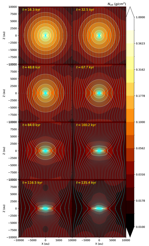
Figure 2: Formation of a pseudodisk in time, $B_{0}=30{\mathrm{\,\mu G}}$. The color and white contours show column densities and the cyan lines trace the magnetic field lines at the XZ plane.

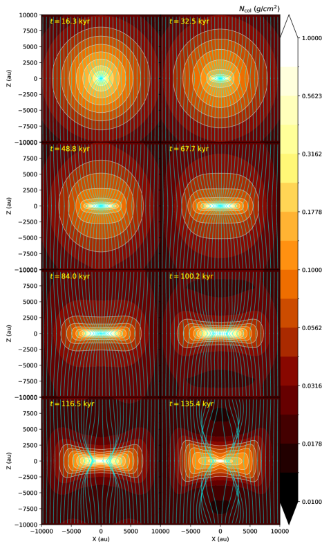
Figure 3: Same as Figure 2 but with $B_{0}=150{\mathrm{\,\mu G}}$.

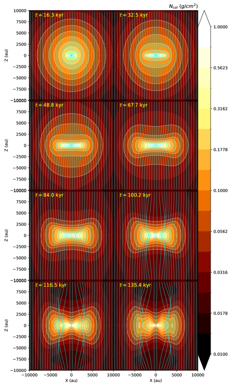
Figure 4: Same as Figure 2 but with $B_{0}=270{\mathrm{\,\mu G}}$.

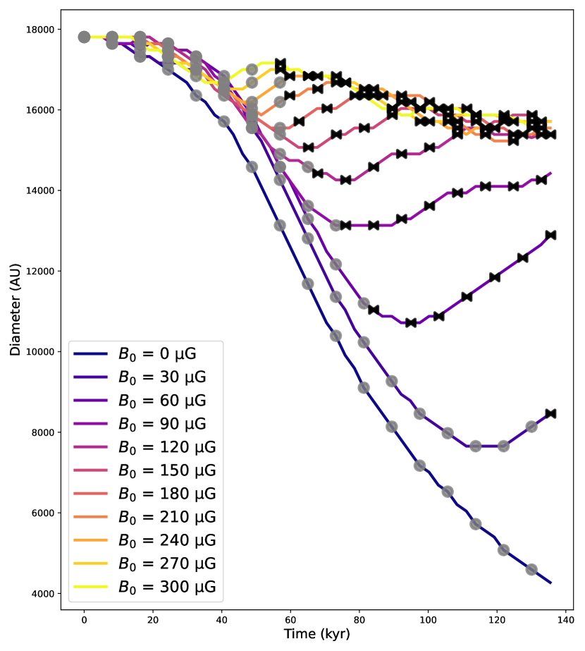
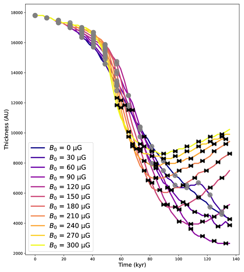
Figure 5: The diameter (left) and thickness (right) of the collapsing core at the threshold density $\rho_{t}=1.6\times 10^{-19}$ g cm^-3. Filled gray circles denote a spheroid shape, black crosses a toroid shape.

In order to quantify the flattening of the isodensity contours in time, we measured the major and the minor axes of the contours at a selected threshold density $\rho_{t}=1.6\times 10^{-19}{{\mathrm{\,g}}}~{}\mathrm{cm}^{-3}$. This threshold density is arbitrarily chosen to highlight the shape of the flattened pseudodisk Figure 5 displays the evolution of the pseudodisk thickness and diameter in time, which are affected by the magnetic field strength. Determining the pseudodisk diameter with a threshold density is justified by observational criteria. In GS93II, the radius of the pseudodisk was determined from the convergence of trajectories of fluid elements in the ballistic approximation. In our simulations, however, the existence of the isothermal pressure force term in equation (2), $-c_{\mathrm{s}}^{2}\nabla\ln\rho$, removes the sharp convergence of streamlines found by GS93II.

Seen clearly in Figure 5, the appearance of toroid features corresponds to the stage where the diameter of the pseudodisk stops shrinking and starts to increase. We note that the diameter of the pseudodisk starts to increase earlier for stronger $B_{0}$. The minimum diameter corresponds to the minimum of mass-to-flux ratio as shown in Figure 8. After this increase, and during the remaining evolution, the diameter has an oscillatory behavior, reflected also in the mass, the flux, and mass-to-flux ratio (see Figure 8).

3.2 Magnetic field lines

The behavior of magnetic fields during the collapse process is strongly dependent on their initial strength, as coupling of the magnetic forces with the flow governs the stiffness of the field. Strong magnetic force acts against the collapse, and as it happens, the field is dragged to a lesser extent along the flow. As expected, the magnetic field rapidly acquires an hourglass morphology during collapse. The increase of the resistivity with density at the center, softens the magnetic field kinks in this region.

Figure 6: As in Figure 1, with cyan lines still tracing magnetic field lines, but displaying electrical current density $j_{\mathrm{tot}}=|\mathbf{j}|$ distributions, and the view is zoomed closer to the center.

Given the presence of sharply pinched angles in the midplane, we inspect the presence of current sheets. Calculating the electrical current density $\mathbf{j}$, we find that $\mathbf{j}$ is generally distributed like a current sheet as shown in Figure 6 for the models shown in Figure 1. The current sheet becomes thicker and stronger with increasing magnetic field, acquiring a bowtie shape ${\blacktriangleright\mspace{-10.0mu}\blacktriangleleft}$.

The maximum magnetic field strength in the system reaches up to $\sim 12$–$14\,\mathrm{mG}$, with $B_{0}=30\mathrm{{\mathrm{\,\mu G}}}$. The systems with initially weakest fields gather strongest fields over time as the field is dragged toward the center. On the other hand, initially strong fields decrease from their maximum value by several $\mathrm{mG}$ during their continued development.

3.3 Mass Accretion Rates

Figure 7 shows the mass accretion rate into the sink particle as a function of time. In general, the accretion rate peaks soon after the collapsing material starts falling toward the centre; then, it gradually decreases. The strong initial accretion is an effect of the initial high mass of the central point that drives the collapse. The decrease of the mass accretion rate is also expected given the initial density profile that decreases with radius, and that there is no mass inflow from the boundaries, so the material runs out. Because our simulations do not start from equilibrium condition, we can reasonably expect higher accretion rates than in Shu (1977). The Shu (1977) model predicts a constant accretion rate $\dot{M}=m_{0}\mathrm{c}_{\mathrm{s}}^{3}/G=0.975\mathrm{c}_{\mathrm{s}}^{3}/G$ (See Shu 1977, Equation (8) and Table 1) where in the case of our sound speed, $\dot{M}=9.9\times 10^{-6}\,{M_{\sun}}\,{\mathrm{\,yr}}^{-1}$. This is withing the range of values of Figure 7, but smaller than the most rapid measured accretion rates. The accretion behavior is clearly affected by magnetic field strength. Stronger fields decrease the accretion rate faster after the initial peak because the stronger fields restrict the mass accretion across the field lines. Toward the end, the accretion rate increases as the magnetic systems reach unstable states, generally weakening the strength of the field toward the central sink. However, in the case without magnetic field, the gradual decrease of the accretion rate continues until the very end.

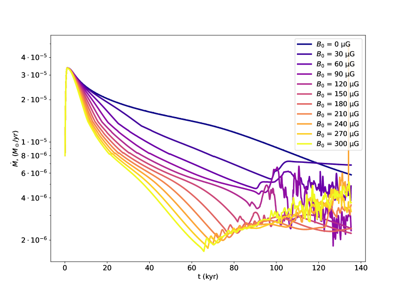
Figure 7: Mass accretion rates of all the systems as a function of time.

3.4 Spherical Mass-to-flux ratio

We calculate the nondimensional spherical mass-to-flux ratio $\lambda$ defined as

$$\lambda=2\pi G^{1/2}\frac{M(R_{\Phi})}{\Phi(R_{\Phi},0)},$$ (6)

following Li & Shu (1996). The flux $\Phi(R_{\Phi},0)$ was measured through a circular surface at the equator ($z=0$) with a constant radius of $R_{\Phi}$. The corresponding mass $M(R_{\Phi})$ is the mass enclosed within a sphere of radius $R_{\Phi}$, where $M(R_{\Phi})$ includes both mass of the gas and of the central object.

Figure 8 shows the evolution of $\lambda$ for all systems over time. We chose $R_{\Phi}=5000\,{\mathrm{\,au}}$. Generally we see a linear decrease of $\lambda$ from the initial state. This is followed by small amplitude oscillations toward a more constant value. The decrease in $\lambda$ is due to the assumed initial condition, where the magnetic field is uniform and the density is centrally concentrated, therefore $\lambda$ decreases with radius. As accretion to the central source proceeds, it brings in material from the outside with smaller values of $\lambda$. This is shown by the change in the magnetic flux as a function of time (see Figure 8b). The growth of magnetic flux is inversely influenced by the strength of the initial magnetic field: the weaker the magnetic field, the stronger the flux can grow relatively to its initial state. This is directly related to the fact that the weakest magnetic field is the easiest to drag, with less magnetic forces opposing the flow. In the case of $B_{0}=30\,{\mathrm{\,\mu G}}$ a maximum flux is not yet reached within the simulation runtime. The oscillation of the flux and of $\lambda$, particularly visible for the strong $B_{0}$, are caused by the back reaction of the magnetic field on the gas, as the magnetic field resists to be dragged to the center and the magnetic pressure builds up, causing the temporary expansion of both the field lines and the gas. Thus, the dragging of field and gas to the center happens in this oscillatory fashion (see Figure 8d).

Figure 8: Time evolution of the mass-to-flux ratio $\lambda$. The flux is calculated at the midplane within a radius $R_{\Phi}=5000{\mathrm{\,au}}$, for different values of the initial magnetic field. Panel (a) a has the total mass within the $R_{\Phi}=5000{\mathrm{\,au}}$ radius from the center including the sink particle. Panel (b) shows the evolution of the magnetic flux with time. Panel (c) displays $\lambda$ for all $B_{0}$. Panel (d) shows $\lambda$ for $B_{0}=180-300\,{\mathrm{\,\mu G}}$ to highlight the oscillation effect.

3.5 Shock detection

As pseudodisks result from anisotropic supersonic inflow, it is relevant to ask whether there are shocks present in the system. When examining our simulations, we find a supersonic inflow that bends and collides close to the disk midplane near the inner surfaces of the flattened density profiles. These regions would be the places to look for shocks. Toward this goal, one can find the locations of compression, or where there is a quick transition in velocity.

Figures 9 and 10 show a representative case of a shock detection. While details can be different, the general case applies to all simulations where toroidal pseudodisks form. There is a general supersonic inflow, which transitions from subsonic to supersonic at the edges of expanding inside-out collapse wave. The flow converges toward the midplane and the pseudodisk with a supersonic infall. Near the pseudodisk, shown in Figure 9 at 78.56 kyr, there appears a sharp transition from supersonic to subsonic flow. This transition layer is a natural location for shocks, and it appear as the toroidal pseudodisk forms. As shown in Figure 10 these transition layers correlate with regions with a high degree of compression as traced by both negative divergence of velocities and density gradients.

Because these tracers – deceleration of flow velocity from subsonic to supersonic, density gradients and compression – correlate on pseudodisk surfaces, we judge that there are shocks present in our simulation. However, the scale of these features is smaller than the grid scale, and cannot be resolved.

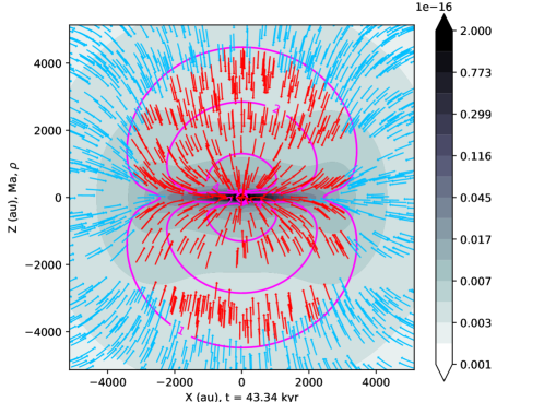
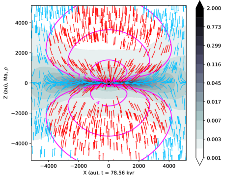
Figure 9: Examining potential shock location in pseudodisk surfaces in B150 with $B_{0}=150{\mathrm{\,\mu G}}$ at early and late stages. The purple line contours show the regions where the velocity at Mach numbers 1, 2, 4 and 8. The red arrows trace supersonic flows, the blue arrows indicate subsonic speeds, and the grey contours trace density.

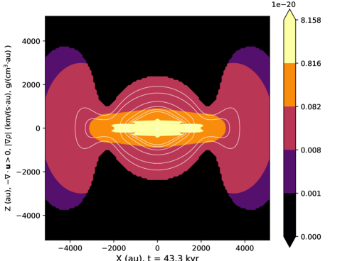
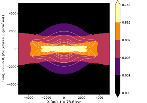
Figure 10: Same frames as Figure 9, but displaying areas with great velocity convergence (white contours) and density gradients (color contours) as contributing tracer for inflow shocks. The white contours trace the velocity convergence levels $\big{[}0.02,0.04,0.09,0.13,0.17,0.22\big{]}\,{\mathrm{\,km}}/({\mathrm{\,s}}\,{\mathrm{\,au}})$.

4 Code test and performance

4.1 Comparison to ZeusTW model

To compare our results against a more established numerical scheme, we constructed a 2-D axisymmetric model using ZeusTW (Krasnopolsky et al. 2010, 2012), with properties comparable to those of our Astaroth model except in following respects. First, the featured ZeusTW model is only two-dimensional and it uses spherical coordinate system instead of Cartesian one. Therefore, it can be expected to keep general symmetry better then the 3-D Cartesian simulation. Second, it is a low order code, being more numerically diffusive. Third, the central sink method is different as it is based on an inner boundary condition for inflowing fluid. Therefore, the sink mechanism of Astaroth is within the grid, whereas in ZeusTW the sink is external to the grid itself.

Figure 11 shows Astaroth and ZeusTW frames at a comparable time. Column densities from the ZeusTW model have been calculated with Perspective (Väisälä et al. 2019). There is a difference in the column density levels, due to different domain size and shape, but local density levels are comparable. The results are in qualitative agreement, and the time evolution shows essentially the same progress, with pinching of the field and formation of a thin flat pseudodisk. One difference is caused by the sink method, which in Astaroth case creates a small bulge surrounding the sink particle. Another difference is in favour of Astaroth as the higher order code can handle a much sharper pinch in the magnetic field, whereas the ZeusTW starts losing its initial pinch.

Figure 11: Left side shows Astaroth and right side ZeusTW+Perspective results at corresponding times. Contours and curves represent column density and magnetic field lines as in Figure 1. There is difference in column density contour levels because of different domain shape and size.

4.2 GPU Performance

Astaroth code performance has been benchmarked in Väisälä et al. (2021) and Pekkilä et al. (2022). They conclusively demonstrate the performance benefit of the GPU implementation. For example, according to Väisälä et al. (2021), a single GPU device could perform about $10\times$ faster than a 40-core CPU node. Clear performance benefit from the use of GPUs in comparison to more traditional CPU parallel computing is to be expected, as it is has been demonstrated by most GPU codes (see e.g. Benítez-Llambay & Masset 2016; Grete et al. 2021; Schive et al. 2018). With Astaroth in particular, the high order of this computation adds to the stencil size and, therefore, to the cost of each step due to memory access latencies; which was challenging in the initial development (Pekkilä et al. 2017) but has been later solved (Pekkilä 2019).

Pekkilä et al. (2022) benchmarked scaling of the typical multi-GPU and multinode Astaroth. When examining performance of Astaroth on a GPU node they measured that the speedup was 18–53$\times$ the performance of the Pencil Code on a CPU node. When running the code on 16 nodes the gained speed up was 20–60$\times$ at best, using the largest grid size, with $N=1024^{3}$. Other than speedup, they also compared energy efficiency with performance per watt. In that case, as single node Astaroth was 8–11$\times$ more energy efficient then the Pencil Code CPU comparison. On 16 nodes, 9–12$\times$ improved energy efficiency was measured at the largest grid size. There reason why the largest problem size performs the best is because it reduces the relative proportion of communication latency between multiple GPUs, with system being closer to compute-bound than communication-bound conditions when relatively large number of grip points are allocated per GPU.

However, those are not based on a completely identical setup to the one used here, as our addition of shock viscosity and sink particle do add further performance demands, due to shock viscosity in particular requiring multiple stencil operation steps. Therefore, in this work we focus on examining the code scaling with the properties we utilize.

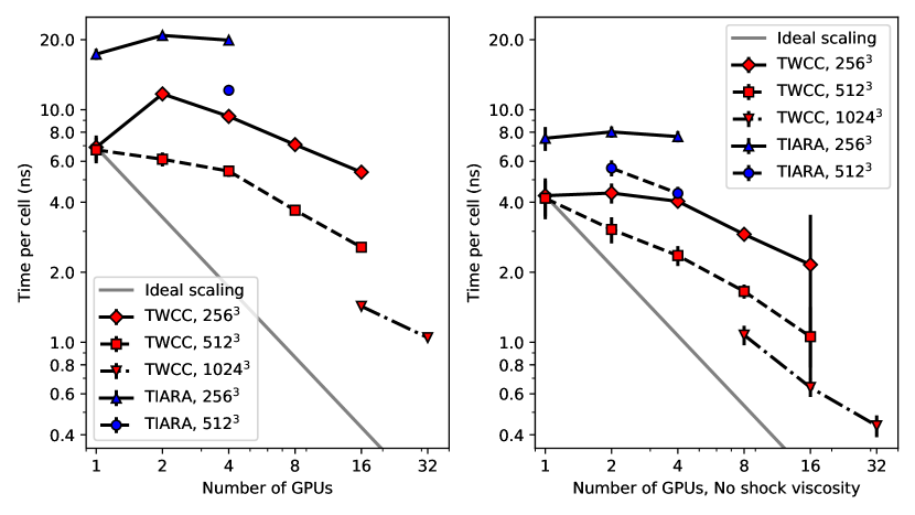
Figure 12: Strong scaling. Performance is measured with fixed grid size while the number of GPUs is changed, both with (left) and without (right) shock viscosity. Error bars show the standard deviations of the measurement. Time per cell refers to the time taken to calculate a single time step normalized by the number of cells in the simulation. TWCC refers to Taiwan Computing Cloud, and TIARA is the TIARA GP cluster of ASIAA.

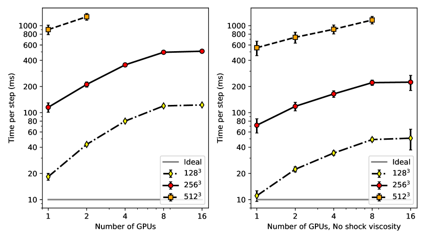
Figure 13: Weak scaling, on TWCC. Problem size per GPU is kept fixed ($128^{3}$, $258^{3}$ or $512^{3}$ per GPU), both with (left) and without (right) shock viscosity. The estimated wall-clock time per step is shown without normalization by the number of cells.

Figure 12 shows strong scaling with the computational loop under a set of resolutions and available GPUs. First thing we can notice is that with the primary resolution of the modeling work presented in this study, $256^{3}$, a single GPU simulation run can be seen to be very economical. This is due to the small grid and lack of device-to-device communication. While it is true that at 16 GPUs the system is faster performance-wise, the gain is not enough to justify the device count. However, many GPUs can be justified at higher resolutions due to performance and memory requirements. At $512^{3}$ 8–16 GPUs could be considered a reasonable choice, and with $1024^{3}$ resolution, at least 16 GPUs is essentially mandatory. The strong scaling follows comparable slopes in all cases past 4 GPUs where doubling the GPU number provides about 1.4–1.6$\times$ increase in performance. In the most compute bound $1024^{3}$ case, without shock viscosity, scaling approaches about 1.7$\times$ speedup, with the theoretical limit being 2$\times$ with the same increase of GPUs.

Benchmarks were performed with and without shock viscosity included in the operations. Roughly speaking, the inclusion of shock viscosity would double the needed computing time. This is likely because shock viscosity requires a series of operations with several passes with device to device communication and very large smoothing stencil. Regardless, the cost of the performance loss is worth it due to much increased model stability.

TWCC performs substantially better than the TIARA GP nodes. Reason for this difference is in hardware, as TIARA GP has earlier generation P100 GPUs in use while TWCC features more recent V100 GPUs with larger availability of parallel GPUs overall.

Figure 13 shows the behavior of weak scaling. Weak scaling follows the expected behavior where at first the added communication overhead increases the required computing time, but this behavior starts to plateau at higher number of GPUs. Weak scaling improves with larger problem size per GPU in the range from $128^{3}$ through $\gtrsim 512^{3}$, which fit within device memory.

Our numbers, however, are not exactly the same as the ones featured in Pekkilä et al. (2022). This is understandable, because we do not measure exactly the same things. Our aim has been to process a full computational loop as it is in the problem solved in this study. In addition to shock viscosity this includes global reduction operations required for calculating the Courant time step, and calculating the accreted mass to the sink particle.

Regardless, performance benefits can be experienced in a practical way. In our case, one $256^{3}$ simulation took about ten hours on a single GPU to be completed. With multiple available GPUs one could compute all our production runs practically overnight. However, if we assume that $10\times$ speedup estimate of Väisälä et al. (2021), then similar operation would have taken more than roughly 4 days on a series of CPU-nodes.

5 Implications

5.1 Observational considerations

All of our models show a pinched magnetic field. To get a simple estimate of how the field would be visible in a sub-millimeter polarization map, we calculate the polarization of an edge-on core following the method of Fiege & Pudritz (2000). With this method we calculate the column density $\Sigma$ and the corresponding Stokes parameters $Q$ and $U$, assuming an optically thin system. $Q$ and $U$ are subsequently used to get a polarization angle $\chi$, which is tilted 90 degrees to trace the projection of the plane of the sky magnetic field. This type of calculation is only dependent on the integrated column density and the magnetic field orientation. As such, the method of Fiege & Pudritz (2000) is a very simplified and should not be confused with more sophisticated radiative transfer model. However, it can provide a quick representation of a magnetically aligned dust polarization pattern.

Figure 14 features a typical example of a pinched hourglass magnetic field seen in the polarization map calculated from our model. Figure 15 shows similar image for strong magnetic fields. The pinch of the field become less visible for a larger value of the initial magnetic field and the pinch is stronger toward the edge. Similar polarization patterns are seen from various observations.

Our model is focused on the pseudodisk and therefore its limits have to be acknowledged. Our comparison can only apply to the protostellar envelope since our model does not include rotation and, thus, it cannot produce a protostellar disk or an outflow.

Apart from HL Tau described in Introduction there are many other objects with pseudodisk candidates, and are discussed below. Even though these observed sources have protostellar disks and outflows, we are interested in discussing their large scale pseudodisk structures.

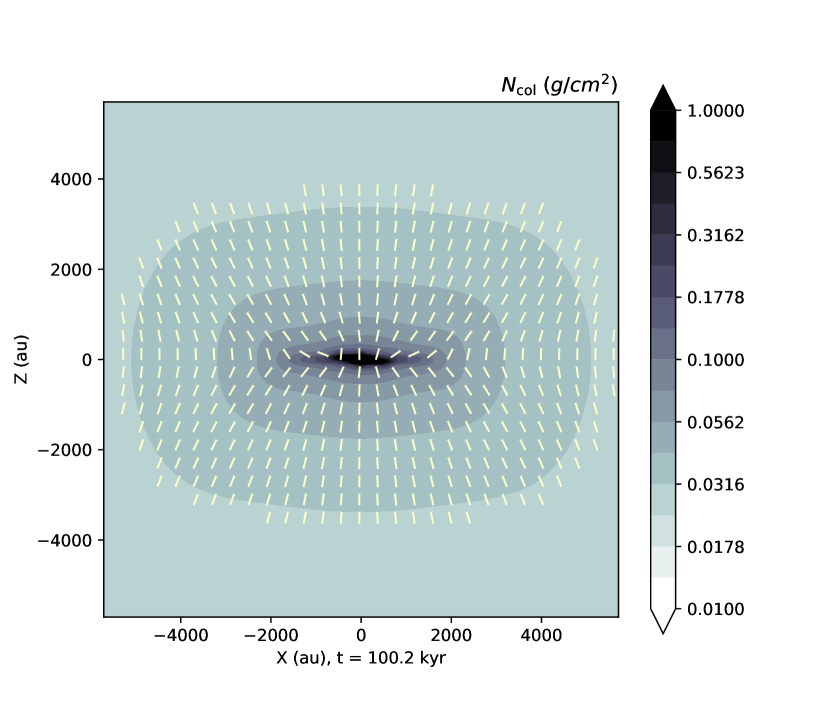
Figure 14: Polarization map following Fiege & Pudritz (2000) method, depicting the case B030, with vectors matching the direction of the plane of sky magnetic field. Polarization vectors are only shown over a column density threshold for readability.

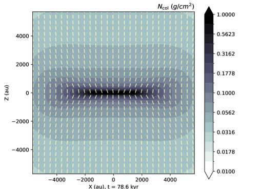
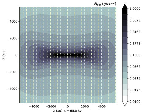
Figure 15: Same as Figure 14 but with the cases B150 (top) and B270 (bottom).

NGC1333 IRAS 4A: a pseudodisk model has also been applied to the polarization map of NGC1333 IRAS 4A (Gonçalves et al. 2008). They concluded that the envelope of NGC1333 IRAS 4A can be well fitted with a GS93I-type pseudodisk model from which a magnetic field strength can be estimated. Recently, Ko et al. (2020) has obtained further polarization maps at sub-millimeter frequencies. At large scales, all the maps show the pinched magnetic field geometry, except for the 6.9 mm map where the polarization angle differs by 90 degrees. This difference is explained as an effect of foreground extinction.

L1448 IRS2: The magnetic field geometry derived from Kwon et al. (2019) has an hourglass morphology and a substantially flattened density structure with size scales matching pseudodisks, i.e., $\sim 1000-2000$ au. Such large-scale effects match well with a pseudodisk scenario, and being a Class 0 object, L1448 IRS2 is at a stage where a pseudodisk would be expected to be present. However, there have to be other contributions to explain the observed depolarization close to the system’s central plane. Kwon et al. (2019) state that the depolarization can be caused e.g. by disturbances of the inner environment by an outflow. However, both pseudodisk and outflow can exist in the same system.

L1157: This source has also the characteristics of a pseudodisk with an outflow pushing out from the center. Looney et al. (2007) discovered a flattened envelope structure seen in infrared absorption surrounding the bright central outflow. This structure is large and relatively diffuse in approximately 15000 to 30000 au in size. While this is larger than a pseudodisk of our model, pseudodisk formation on larger scale is not uncalled for, as long as the magnetic fields maintain a relative coherence with respect to the collapse. Molecular line explorations of this object by Chiang et al. (2010) discovered a strong in-flowing velocity profile at the scale of the elongated envelope, as is expected in pseudodisks. In addition, the inner envelope mapped at $8\,\mu\mathrm{m}$ and in $\mathrm{N}_{\mathrm{2}}\mathrm{H}^{\mathrm{+}}$, being close to size of $\sim 2000\,{\mathrm{\,au}}$, approaches the pseudodisk scales of our models. This system potentially demonstrate the multiscale nature of the pseudodisk phenomenon from more diffuse to dense gas. There is still accretion toward the central protostar. The polarization observations by (Stephens et al. 2013) show an hourglass morphology of the magnetic field.

B335: This source has polarization vectors that indicate a strongly pinched nad organized hourglass magnetic field from from $1000\,{\mathrm{\,au}}$ to from $50\,{\mathrm{\,au}}$ scales (Maury et al. 2018), which matches a typical pseudodisk scale. The radial velocity observations imply that rotation is weak at all scales, with the majority of observed kinematics behaving as inflow (Saito et al. 1999; Yen et al. 2010, 2015). Cabedo et al. (2023) found that the ionization fraction is sufficiently high to ensure a good coupling between the field and the gas. Therefore, B335 appears as an almost textbook case where the magnetic field dominates the gas dynamics. This does not mean that there is no rotation, but at large scales rotation is not the most dynamically relevant feature.

HH211: this source displays the typical behavior of a magnetized collapse (Lee et al. 2019): it has a collapsing inflow and a pinched hourglass magnetic field. Yen et al. (2023) have performed further estimates and analysis on its structure, kinematics, and magnetic field both at the envelope scale and at the disk scale. The HH211 system displays a pinched magnetic field configuration with a flattened toroid-like envelope, with a significant inflow. Based on their estimates, the magnetic field properties of HH211 are such that they indicate a presence of a diffusive process such as ambipolar diffusion. The larger envelope still maintains a $r^{-2}$ density distribution, indicating its relatively young age since the collapse has not produced sufficient flattening on the largest scale.

As can be seen from this list of candidate objects, it is possible to study several pseudodisk-like protostellar envelopes. With further improvement, our models will be able include both more complicated physics and a range of physical scales, so that e.g. both a pseudodisk and a protostellar disk can exist in the same model. This will allow us to address the details seen in the observed systems more comprehensively.

5.2 Implications to Early Models

GS93I and II found the basic mechanism for the formation of a pseudodisk, where the magnetic field that opposes the collapse and bends during the process, deviates the gas flow toward the equator creating a disklike density concentration. The GS93II simulation allowed for longer period of time, compared to GS93I, where the pseudodisk flattened until artificial reconnection effects near the center became too strong. However, it is noteworthy that while GS93I assumes an isothermal equation of state, as does our model, the numerical model of GS93II leaves the pressure force out of the calculations. Our inclusion of isothermal pressure appears to lead to changes in the convergence of inflow within the pseudodisk, as pressure maintains a finite scale height of the density distribution. The effect is present even without any kind of nonisothermal equation of state. Our low magnetic field cases are closest to the GS93II results. In that case we get a relatively flat pseudodisk with sharply bent magnetic field. With increasing magnetic field strength, the pseudodisk is larger and thicker and the effects of pressure and compression start to appear. Therefore, the density distribution has a more stratified structure. During the dynamical evolution of our models, there are stages in which the isodensity contours are similar to the isothermal toroids of Li & Shu (1996) and to those found in the simulations of Allen et al. (2003) who studied the magnetized collapse of a cloud core without rotation, which also lead to the formation of pseudodisks. Even though the mass-to-flux ratio is different in these two latter works and in our simulation, it seems that the toroid stage is a robust structure that appears during the evolution magnetized cloud cores.

5.3 Infall Shocks

The existence for large-scale infall and accretion shocks during the star-forming process has been a long-standing question. Yorke et al. (1993, 1995), and Yorke & Bodenheimer (1999) presented the earliest cases in their hydrodynamic simulations. These shocks are expected to produce sharp density and velocity contrasts. Recent observations have found shock signatures of infalling material through the emission of SO and SO₂ (Garufi et al. 2022).

In Section 3.5 we show the likely presence of infall shocks in our systems with $B_{0}=150\,{\mathrm{\,\mu G}}$. The inflowing gas is strongly oriented along the magnetic field lines: the low-density inflowing medium accelerates along the field direction and becomes supersonic until it is slowed down and deflected at the shock surface, where there are signs of both velocity deviation and density compression. Detecting shocks within a supersonic system where flows collide is not surprising. What is uncertain is the real strength of the shocks, and how much thermal emission would be generated due to viscous heating in those shock interactions. For example, Yorke & Bodenheimer (1999) calculated the thermal emission of shocks formed by material inflowing onto a disk surface. Such a calculation is beyond the scope of this paper.

6 Summary

We have performed simulations of the collapse of a nonrotating, uniformly magnetized cloud core, using the high-order GPU code Astaroth. A pseudodisk naturally forms for different strengths of the poloidal magnetic field. The collapse was examined with ten different levels of initial magnetic field strength $B_{0}$, keeping the same initial density profile and central mass. Our conclusions are summarized below.

(1) We find that density distribution evolves from spheroidal to toroidal through the time evolution. The degree of central flattening of the final configurations decreases with the value of the initial magnetic field. Toroids are favored in the case of stronger magnetic field, while spheroids/flattened pseudodisks result in the case of weaker fields.

(2) The mass accretion rate on the central object increases rapidly at first, and then decreases over time following a power-law type behavior, as the surrounding cloud is depleted. At late times, mass accretion occurs in an oscillatory fashion due to the back reaction of the compressed magnetic field on the flow. The stronger the field, the faster is the decrease of the accretion rate, and the earlier the oscillatory behavior sets in.

(3) The spherical mass-to-flux ratio $\lambda$ does not stay constant during the evolution. Because of the initial nonuniform mass-to-flux ratio, the buildup of the flux is much more rapid than that of the mass, leading to a decrease in $\lambda$ with time. Furthermore, after the initial decrease, $\lambda$ approaches a constant value with small oscillations, due to the back reaction of the field on the gas.

(4) Infall shocks are produced where the low density medium inflowing along magnetic field lines accelerates to supersonic speed until it is slowed down and deflected at a shock located at the surface of the pseudodisk.

We find that the code Astaroth can now produce pseudodisk from a basic principles, and this can function as a foundation for more sophisticated models in the future, where additional physical processes can be added. For example, a further implementation of a Poisson solver can allow for inclusion of self-gravity. Additionally, more complicated nonideal MHD mechanisms like ambipolar diffusion can be introduced. Rotation can also be included to follow the formation of a centrifugally supported disk at a a scale much smaller than the pseudodisk. To investigate these inner protostellar disks, the resolution has to be increased and the grid made nonequidistant.

Appendix A Shock viscosity

In addition to resistivity and kinematic viscosity, an artificial shock capturing viscosity is needed. Shock viscosity is a required property near the center of the collapse where velocities can get highly supersonic. However, it has little effect on the general behavior of the collapse process, with the effects of shock viscosity being local and not global. In Equation (2), $\zeta_{\mathrm{shock}}$ is an artificial viscosity parameter computed as follows. It is based on the method used by the Pencil Code and presented by Gent et al. (2020). First, we get a scalar field $u_{-D}$ by calculating negative divergences while setting every nonnegative diverge value to zero.

$$u_{-D}=(-\nabla\cdot\mathbf{u})_{+}$$ (A1)

Second, we get a scalar field $u_{5}$ by picking maximum within the points in

$$u_{5}(i,j,k)=\mathrm{max}[u_{-D}(i-2\ldots i+2,j-2\ldots j+2,k-2\ldots k+2)],$$ (A2)

where $i$, $j$ and $k$ are the local grid indices. As the last step we perform smoothing on $u_{5}$ with a normalized $7\times 7\times 7$ window with Gaussian weights $w(i)=[1,9,45,70,45,9,1]$ in each direction to get scalar field $f_{\mathrm{shock}}$, and from there we finally get

$$\zeta_{\mathrm{shock}}=f_{\mathrm{shock}}\mathrm{min}(\Delta x,\Delta y,\Delta z)^{2},$$ (A3)

which is then used as an equation term.

Appendix B Sink particle method

The sink particle method was inspired by Lee et al. (2014). However, the method we implemented is not identical to theirs, for two main reasons. First, some aspects of Lee et al. (2014) implementation are not GPU/Astaroth DSL friendly. Secondly, we found that if implemented as described in the paper, the method would not result in numerically stable results.

The sink particle effects appear in three terms within the system of equations, with $S_{M}$ in Equations (1) and (2), and $\mathbf{g}$ in Equation (2). The mass accretion is performed by

$$S_{M}(\ln\rho,\Delta t)=\frac{\rho-\rho_{\mathrm{sink}}}{\Delta t}$$ (B1)

within the sink radius $R_{\mathrm{sink}}=2\Delta x$, if $\rho-\rho_{\mathrm{sink}}>0$. $\Delta t$ is the length of the time step and $\rho_{\mathrm{sink}}$ is the value of Equation (4) at $r=2R_{\mathrm{sink}}$. Due to the numerical method, $\rho=\exp(\ln\rho)$. During the code testing we found that a fixed density roof inside the sink particle radius, respective of the initial condition as above, would be most beneficial in terms of the system stability. If, e.g., $\rho_{\mathrm{sink}}=0$, this would cause a huge density discontinuity at the sink particle boundary resulting in strong numerical instabilities. The $S_{M}$ term in Equation (1) takes care of the loss of momentum by the mass accretion.

The mass accumulation requires a GPU specific implementation. CUDA kernel operations are performed in multiple threads, and those threads cannot communicate with each other during the kernel runtime. We include an accretion buffer, which collects mass accumulation via each thread. At the end of a time step, accumulated masses per grid element are computed together by Astaroth collective diagnostic operations, and that mass is added to the sink particle, $M_{*}$.

The mass of the sink particle functions as a central attractor, which contributes to the gravitational term in Equation (2),

$$\mathbf{g}(r)=-\frac{GM_{*}}{r^{2}}\mathbf{\hat{r}},$$ (B2)

active in the domain where $R_{\mathrm{sink}}<r<R_{\mathrm{max}}=9300{\mathrm{\,au}}$. Setting a maximum gravity radius, reduces significantly all problematic effects caused by the corners of a Cartesian domain. In particular, these effects include pronounced disturbances on the symmetry of the collapsing cloud and numerical instability in the domain corners which are greatly reduced when applying the $R_{\mathrm{max}}$ limit. In addition, without the $R_{\mathrm{max}}$ limit the system corners have a tendency to become numerically unstable. $R_{\mathrm{max}}$ is slightly smaller than the maximum possible radius, because that was deemed beneficial during the testing stage.

It should be noted that we use the central mass as the only source of gravitational force, i.e., we ignore the self-gravity of the infalling gas. The initial Bondi radius is $GM_{\rm sink}/c_{s}^{2}=12700{\mathrm{\,au}}$, which is larger than $R_{\mathrm{max}}$. Therefore the computational box is enclosed in the gravitational “sphere of influence” of the sink particle and the calculation is self-consistent. We have built this model as being dominated by a central mass, because for this proof of concept study, a Poisson equation/self-gravity solver has been out of the scope. However, in future work, as a self-gravity solver for Astaroth will develop to a functional stage, self-gravity will be included into the models.

References

- Aalto University (2023) Aalto University. 2023, The Astaroth Repository, Espoo, Finland
- Allen et al. (2003) Allen, A., Shu, F. H., & Li, Z.-Y. 2003, ApJ, 599, 351
- ALMA Partnership et al. (2015) ALMA Partnership, Brogan, C. L., Pérez, L. M., et al. 2015, ApJ, 808, L3
- Benítez-Llambay & Masset (2016) Benítez-Llambay, P., & Masset, F. S. 2016, ApJS, 223, 11
- Brandenburg (2003) Brandenburg, A. 2003, Computational Aspects of Astrophysical MHD and Turbulence, Advances in Nonlinear Dynamos, ed. A. Ferriz-Mas & M. Núñez, 269
- Cabedo et al. (2023) Cabedo, V., Maury, A., Girart, J. M., et al. 2023, A&A, 669, A90
- Chiang et al. (2010) Chiang, H.-F., Looney, L. W., Tobin, J. J., & Hartmann, L. 2010, ApJ, 709, 470
- Ciolek & Königl (1998) Ciolek, G. E., & Königl, A. 1998, ApJ, 504, 257
- Dobler et al. (2006) Dobler, W., Stix, M., & Brandenburg, A. 2006, ApJ, 638, 336
- Fiege & Pudritz (2000) Fiege, J. D., & Pudritz, R. E. 2000, ApJ, 544, 830
- Galli & Shu (1993a) Galli, D., & Shu, F. H. 1993a, ApJ, 417, 220
- Galli & Shu (1993b) —. 1993b, ApJ, 417, 243
- Gardiner & Stone (2005) Gardiner, T. A., & Stone, J. M. 2005, Journal of Computational Physics, 205, 509
- Garufi et al. (2022) Garufi, A., Podio, L., Codella, C., et al. 2022, A&A, 658, A104
- Gent et al. (2020) Gent, F. A., Mac Low, M. M., Käpylä, M. J., Sarson, G. R., & Hollins, J. F. 2020, Geophysical and Astrophysical Fluid Dynamics, 114, 77
- Gonçalves et al. (2008) Gonçalves, J., Galli, D., & Girart, J. M. 2008, A&A, 490, L39
- Grete et al. (2021) Grete, P., Glines, F. W., & O’Shea, B. W. 2021, IEEE Transactions on Parallel and Distributed Systems, 32, 85
- Harris et al. (2020) Harris, C. R., Millman, K. J., van der Walt, S. J., et al. 2020, Nature, 585, 357
- Hayashi et al. (1993) Hayashi, M., Ohashi, N., & Miyama, S. M. 1993, ApJ, 418, L71
- Hunter (2007) Hunter, J. D. 2007, Computing in Science & Engineering, 9, 90
- Käpylä et al. (2018) Käpylä, M. J., Gent, F. A., Väisälä, M. S., & Sarson, G. R. 2018, A&A, 611, A15
- Ko et al. (2020) Ko, C.-L., Liu, H. B., Lai, S.-P., et al. 2020, ApJ, 889, 172
- Krasnopolsky & Königl (2002) Krasnopolsky, R., & Königl, A. 2002, ApJ, 580, 987
- Krasnopolsky et al. (2010) Krasnopolsky, R., Li, Z.-Y., & Shang, H. 2010, ApJ, 716, 1541
- Krasnopolsky et al. (2012) Krasnopolsky, R., Li, Z.-Y., Shang, H., & Zhao, B. 2012, ApJ, 757, 77
- Kwon et al. (2019) Kwon, W., Stephens, I. W., Tobin, J. J., et al. 2019, ApJ, 879, 25
- Lappi (2021) Lappi, O. 2021, Master’s thesis, Faculty of Science and Engineering, Åbo Akademi University, Turku, Finland
- Lee et al. (2014) Lee, A. T., Cunningham, A. J., McKee, C. F., & Klein, R. I. 2014, ApJ, 783, 50
- Lee et al. (2019) Lee, C.-F., Kwon, W., Jhan, K.-S., et al. 2019, ApJ, 879, 101
- Li & McKee (1996) Li, Z.-Y., & McKee, C. F. 1996, ApJ, 464, 373
- Li & Shu (1996) Li, Z.-Y., & Shu, F. H. 1996, ApJ, 472, 211
- Looney et al. (2007) Looney, L. W., Tobin, J. J., & Kwon, W. 2007, ApJ, 670, L131
- Maury et al. (2018) Maury, A. J., Girart, J. M., Zhang, Q., et al. 2018, MNRAS, 477, 2760
- McKee et al. (2020) McKee, C. F., Stacy, A., & Li, P. S. 2020, MNRAS, 496, 5528
- McKinney (2010) McKinney, W. 2010, in Proceedings of the 9th Python in Science Conference, ed. Stéfan van der Walt & Jarrod Millman, 56 – 61
- Mellon & Li (2009) Mellon, R. R., & Li, Z.-Y. 2009, ApJ, 698, 922
- Pekkilä (2019) Pekkilä, J. 2019, Master’s thesis, Aalto University School of Science, Espoo, Finland
- Pekkilä et al. (2017) Pekkilä, J., Väisälä, M. S., Käpylä, M. J., Käpylä, P. J., & Anjum, O. 2017, Computer Physics Communications, 217, 11
- Pekkilä et al. (2022) Pekkilä, J., Väisälä, M. S., Käpylä, M. J., Rheinhardt, M., & Lappi, O. 2022, Parallel Computing, 111, 102904
- Pencil Code Collaboration et al. (2021) Pencil Code Collaboration, Brandenburg, A., Johansen, A., et al. 2021, The Journal of Open Source Software, 6, 2807
- Pinto et al. (2008) Pinto, C., Galli, D., & Bacciotti, F. 2008, A&A, 484, 1
- Reback et al. (2021) Reback, J., McKinney, W., jbrockmendel, et al. 2021, pandas-dev/pandas: Pandas 1.2.4, v.v1.2.4, Zenodo, doi:10.5281/zenodo.4681666
- Rincon (2019) Rincon, F. 2019, Journal of Plasma Physics, 85, 205850401
- Saito et al. (1999) Saito, M., Sunada, K., Kawabe, R., Kitamura, Y., & Hirano, N. 1999, ApJ, 518, 334
- Schive et al. (2018) Schive, H.-Y., ZuHone, J. A., Goldbaum, N. J., et al. 2018, MNRAS, 481, 4815
- Shu (1977) Shu, F. H. 1977, ApJ, 214, 488
- Stephens et al. (2013) Stephens, I. W., Looney, L. W., Kwon, W., et al. 2013, ApJ, 769, L15
- Terebey et al. (1984) Terebey, S., Shu, F. H., & Cassen, P. 1984, ApJ, 286, 529
- Tsukamoto et al. (2022) Tsukamoto, Y., Maury, A., Commerçon, B., et al. 2022, arXiv e-prints, arXiv:2209.13765
- Väisälä (2017) Väisälä, M. 2017, PhD thesis, University of Helsinki, Finland
- Väisälä et al. (2021) Väisälä, M. S., Pekkilä, J., Käpylä, M. J., et al. 2021, ApJ, 907, 83
- Väisälä et al. (2019) Väisälä, M. S., Shang, H., Krasnopolsky, R., et al. 2019, ApJ, 873, 114
- Virtanen et al. (2020) Virtanen, P., Gommers, R., Oliphant, T. E., et al. 2020, Nature Methods, 17, 261
- Yen et al. (2015) Yen, H.-W., Takakuwa, S., Koch, P. M., et al. 2015, ApJ, 812, 129
- Yen et al. (2010) Yen, H.-W., Takakuwa, S., & Ohashi, N. 2010, ApJ, 710, 1786
- Yen et al. (2023) Yen, H.-W., Koch, P. M., Lee, C.-F., et al. 2023, ApJ, 942, 32
- Yorke & Bodenheimer (1999) Yorke, H. W., & Bodenheimer, P. 1999, ApJ, 525, 330
- Yorke et al. (1993) Yorke, H. W., Bodenheimer, P., & Laughlin, G. 1993, ApJ, 411, 274
- Yorke et al. (1995) —. 1995, ApJ, 443, 199