Finite Time Analysis of Constrained Actor Critic and Constrained Natural Actor Critic Algorithms

Abstract

Actor Critic methods have found immense applications on a wide range of Reinforcement Learning tasks especially when the state-action space is large. In this paper, we consider actor critic and natural actor critic algorithms with function approximation for constrained Markov decision processes (C-MDP) involving inequality constraints and carry out a non-asymptotic analysis for both of these algorithms in a non-i.i.d (Markovian) setting. We consider the long-run average cost criterion where both the objective and the constraint functions are suitable policy-dependent long-run averages of certain prescribed cost functions. We handle the inequality constraints using the Lagrange multiplier method. We prove that these algorithms are guaranteed to find a first-order stationary point (i.e., $\|\nabla L(\theta,\gamma)\|_{2}^{2}\leq\epsilon$) of the performance (Lagrange) function $L(\theta,\gamma)$, with a sample complexity of $\mathcal{\tilde{O}}(\epsilon^{-2.5})$ in the case of both Constrained Actor Critic (C-AC) and Constrained Natural Actor Critic (C-NAC) algorithms. We also show the results of experiments on three different Safety-Gym environments.

1 Introduction

In recent times, there has been significant research activity on constrained reinforcement learning algorithms, motivated largely from applications in safe reinforcement learning (Safe-RL). The idea here is that each state transition not just receives a single-stage cost indicating the desirability of the action and the resulting next state but also receives additional constraint (single-stage) costs that may account for safety of the chosen action and the resulting next state. The goal then is to minimize a ‘long-term cost’ criterion while ensuring at the same time that the ‘long-term constraint costs’ stay within certain prescribed thresholds. The problem setting could generally involve more than one constraint cost. Problems of Safe-RL can in general be formulated in the setting of constrained Markov decision processes (C-MDP), see HasanzadeZonuzy et al. [2021], Jayant and Bhatnagar [2022], Wachi and Sui [2020]. Altman [2021] provides a textbook treatment on C-MDP. As an example, one may consider the problem of navigation of an autonomous vehicle such as a drone or a self-driving car where the goal is to reach the destination in as short a time as possible while ensuring there are no collisions with obstacles or accidents on the way. Such problems can be well formulated in the setting of C-MDPs. Constrained MDPs find several applications in various diverse domains. Some of these applications include finding optimal bandwidth allocation in resource constrained communication networks, determining strategic building and maintenance policies, safe navigation for self-driving cars, drones and robots, optimal energy sharing strategies in energy harvesting networks etc.

In situations where the system model is unavailable, but one has access to data in the form of tuples of states, actions, rewards, penalties, as well as next states, one may formulate and present constrained reinforcement learning (C-RL) algorithms for finding the optimal policies. An important algorithm in this category is the constrained actor critic (C-AC) algorithm originally presented in Borkar [2005] for the long-run average cost setting but for look-up table representations. In Bhatnagar [2010], Bhatnagar and Lakshmanan [2012], C-AC algorithms with function approximation have been presented and analysed for the infinite horizon discounted cost and the long-run average cost objectives respectively. In Bhatnagar and Lakshmanan [2012], an application of the presented algorithm is also studied empirically on a constrained multi-stage routing problem.

The key idea in the aforementioned algorithms has been to relax the constraints into the objective by forming a Lagrangian and then perform a gradient ascent step in the policy parameter while simultaneously performing a descent in the Lagrange parameter. Note that usual actor critic Konda and Tsitsiklis [2003] or natural actor critic algorithms Bhatnagar et al., [2009] ordinarily require two timescale recursions. This is because these algorithms try and mimic the policy iteration procedure whereby the actor or policy parameter update proceeds on the slower timescale while the critic or value function parameter is updated on the faster timescale. In constrained actor critic and constrained natural actor critic algorithms, one needs to introduce an additional (the slowest) timescale over which the Lagrange multiplier is updated.

In this paper, we carry out a finite time (non-asymptotic) convergence analysis of constrained actor critic and constrained natural actor critic algorithms to find the sample complexity of these algorithms (in the constrained setting). We assume that the system model via the transition probabilities is not known and linear function approximation is used for the critic recursion. A non-asymptotic analysis helps provide an estimate of the number of samples needed for the algorithm to converge as well as helps provide appropriate learning rates for the algorithm. In the case of the C-NAC algorithm, the natural gradient is estimated by linearly transforming the regular gradient by making use of the inverse Fisher information matrix of the policy which is clearly positive definite (Kakade [2001]). It is generally observed that using natural gradients speeds up the performance of these algorithms. To the best of our knowledge, a non-asymptotic convergence analysis of three timescale constrained actor critic and constrained natural actor critic algorithms using linear function approximation has not been carried out in the past.

We summarise our principal contributions below:
(a) We carry out the first finite-time analyses for the Constrained Actor Critic and the Constrained Natural Actor Critic algorithms with linear function approximation in the long-run average cost setting.
(b) We conduct the aforementioned analyses under the general assumption of Markovian sampling using TD(0) for the critic recursion and obtain a sample complexity of $\widetilde{\mathcal{O}}(\epsilon^{-2.5})$ for both algorithms to find an $\epsilon$-optimal stationary point of the performance function.
(c) It is important to note here that the sample complexity of both our constrained algorithms matches exactly the one obtained by Wu et al., [2020] which is also $\mathcal{\tilde{O}}(\epsilon^{-2.5})$ even though the latter has been obtained in the case of two-timescale (unconstrained) regular actor critic algorithms. Further, our setting is more general as we consider random single-stage costs and also constraint costs having distributions that are dependent on the current state, action and next state. This is unlike Wu et al., [2020] where the single-stage reward is assumed fixed for the given current state and action. Our result thus shows that under a random cost structure, with inequality constraints in the formulation, and having three timescale algorithms as a result (instead of two timescale algorithms) has no impact on the sample complexity which we believe is a significant outcome of our study.
(d) We show the results of experiments on three different Safety-Gym environments, namely SafetyPointGoal1-v0, SafetyCarGoal1-v0 and SafetyPointPush1-v0, respectively, where we compare the performance of C-AC and C-NAC with Constrained DQN (C-DQN). For the latter, we incorporate the Lagrange based procedure and update the Lagrange multipliers in the same way as C-AC and C-NAC procedures for a fair comparison. We observe that C-NAC shows the best results on all three settings while C-AC is the second-best performer on two of the three settings. Further, all algorithms satisfy the specified average cost constraint.

Notation: For two sequences $\{c_{n}\}$ and $\{d_{n}\}$, we can write $c_{n}=\mathcal{O}(d_{n})$ if there exists a constant $P>0$ such that ${\displaystyle\frac{|c_{n}|}{|d_{n}|}\leq P}$. To further hide logarithm factors,we use the notation $\tilde{\mathcal{O}}(\cdot)$ . Without any other specification, $\|\cdot\|$ denotes the $\ell_{2}$ norm of euclidean vectors. $d_{TV}(M,N)$ is the total variation norm between two probability measures $M$ and $N$, and is defined as $d_{TV}(M,N)=1/2\int_{\mathcal{X}}|M(dx)-N(dx)|$.

2 Related Work

The Actor Critic Algorithm was first analyzed theoretically for its asymptotic convergence by Konda and Borkar [1999]. This was however for the case of lookup table representations. In the case when function approximation is used, Konda and Tsitsiklis [2003] analyzed the actor critic algorithm for its asymptotic convergence. Kakade [2001] proposed the natural gradient based algorithm. Under various settings, the asymptotic convergence of actor critic algorithms has also been studied in (Kakade [2001], Castro and Meir [2010], Zhang et al., [2020]). In Bhatnagar et al., [2009], natural actor critic algorithms that bootstrap in both the actor and the critic have been proposed and analyzed for their asymptotic convergence.

In recent times, there have been many works focusing primarily on performing finite time analyses of reinforcement learning algorithms. Such analyses are important as they provide sample complexity estimates and non-asymptotic convergence bounds for these algorithms. More recently, such analyses for actor critic algorithms have also been carried out though in the unconstrained (regular MDP) setting. Ding et al. [2020] obtain finite time bounds for a natural policy gradient algorithm for discounted cost MDP with constraints. Wu et al., [2020] show a non-asymptotic analysis of a two time-scale actor critic algorithm assuming non-i.i.d samples and obtain a sample complexity of $\tilde{\mathcal{O}}(\epsilon^{-2.5})$ for convergence to an $\epsilon$-approximate stationary point of the performance function. Hairi et al., [2021] consider a fully decentralized multi-agent reinforcement learning (MARL) setting and show a finite-time convergence analysis for the actor-critic algorithm in the average reward MDP scenario. There have also been other recent works that have analysed Natural Actor Critic Algorithms for their non-asymptotic convergence, see for instance, Cayci et al., [2022], Xu et al., [2020], Khodadadian et al., [2023], Khodadadian et al., [2021], Chen et al., [2022].

Borkar [2005] proposed the first actor-critic reinforcement learning algorithm for constrained Markov decision processes in the long-run average cost setting and proved their asymptotic convergence in the lookup table setting. Bhatnagar [2010] developed and examined the first actor-critic reinforcement learning algorithm incorporating function approximation within the context of an infinite horizon discounted cost scenario, addressing control problems subject to multiple inequality constraints. Bhatnagar and Lakshmanan [2012] presents an actor-critic algorithm in the constrained long-run average cost MDP setting with function approximation that incorporates a policy gradient actor and a temporal difference critic. An asymptotic analysis of convergence is then shown for the proposed scheme.

Zeng et al., [2022] recently showed a finite-time analysis for the non-asymptotic convergence of the natural actor critic algorithm to the global optimum of a CMDP problem in the case of lookup table representations and the infinite horizon discounted cost setting. In this paper, we consider the long-run average cost problem with function approximation, originally presented by Bhatnagar and Lakshmanan [2012]. Here, we consider TD(0) for the critic recursion and use projection for the critic. Further, we present the C-NAC algorithm, where we use natural gradients in the actor recursion along with a TD(0) critic. As mentioned earlier, there are no prior finite time analyses for average cost/reward constrained actor critic algorithms with function approximation , so our work plugs in an important gap that previously existed in this direction.

3 Preliminaries

In this section, we present the C-MDP framework and algorithms that we analyze.

3.1 Constrained Markov Decision Processes

We consider a discrete-time Markov Decision Process with finite state and action spaces. We first explain below the notations used.

$\bullet$ $S$ represents the state space and $A$ the action space. Further, let $A(j)\subset A$ denote the set of feasible actions in state $j\in S$.

$\bullet$ Let $p(s,s^{\prime},a)$ denote the probability of transition from state $s$ to $s^{\prime}$ under action $a$.

$\bullet$ We shall consider only randomized policies $\pi$ in this work. Further, policies are assumed parameterized via a parameter $\theta\in{\cal R}^{d}$. Thus, given $\theta$, $\pi_{\theta}(a|s)$ is the probability of selecting an action $a\in A(s)$ in state $s$.

$\bullet$ The stationary distribution (over states) induced by the policy $\pi_{\theta}$ is denoted $\mu_{\pi_{\theta}}$ or simply $\mu_{\theta}$ (by an abuse of notation) and is assumed unique for any $\theta$.

Let $q(n),h_{1}(n),...,h_{N}(n),n\geq 0$, denote a set of costs that is obtained upon transitioning from state $s_{n}$ to state $s_{n+1}$ under action $a_{n}\in A(s_{n})$. At any time instant $n$, the single-stage costs $q(n),h_{k}(n),k=1,...,N$, do not depend on prior states and actions $s_{m},a_{m},m<n$ given the current state-action pair ($s_{n},a_{n}$). For any $i\in S$, $a\in A(i)$, let $d(i,a),h_{k}(i,a)$ be defined as $d(i,a)=E[q(n)|s_{n}=i,a_{n}=a],h_{k}(i,a)=E[h_{k}(n)|s_{n}=i,a_{n}=a],k=1,...,N$, respectively. We assume that the single stage costs are real-valued, non-negative, uniformly bounded and mutually independent. We assume that all the single stage costs $q(n),h_{1}(n),\ldots,h_{N}(n)$ are absolutely bounded by a constant $U_{c}>0$.

3.2 The Objective and Lagrange Relaxation

Our aim is to minimize $J(\pi)$ where

$$J(\pi) =\lim_{n\rightarrow\infty}\frac{1}{n}\mathbb{E}\big{[}\sum\limits_{m=0}^{n-1}q(m)|\pi\big{]}$$

$$=\sum\limits_{s\in S}\mu_{\pi}(s)\sum\limits_{a\in A(s)}\pi(s,a)d(s,a),$$ (1)

subject to the constraints

$$G_{k}(\pi) =\lim_{n\rightarrow\infty}\frac{1}{n}\mathbb{E}\big{[}\sum\limits_{m=0}^{n-1}h_{k}(m)|\pi\big{]}$$

$$=\sum\limits_{s\in S}\mu_{\pi}(s)\sum\limits_{a\in A(s)}\pi(s,a)h_{k}(s,a)\leq\alpha_{k},$$ (2)

$k=1,...,N$, where $\alpha_{1},...,\alpha_{N}$ are certain prescribed (positive) constant thresholds. We conside here that the Markov process $\{s_{n}\}$ under any given policy is ergodic. Hence, the limits in (1)-(2) are well-defined.

Consider a vector $\gamma=(\gamma_{1},...,\gamma_{N})^{T}$ representing a set of Lagrange multipliers with $\gamma_{1},...,\gamma_{N}\in R^{+}\cup\{0\}$. Now we have a Lagrangian $L(\pi,\gamma)$ that we define as

$$L(\pi,\gamma)$$

$$=J(\pi)+\sum\limits_{k=1}^{N}\gamma_{k}(G_{k}(\pi)-\alpha_{k})$$

$$=\sum\limits_{s\in S}\mu_{\pi}(s)\sum\limits_{a\in A(s)}\pi(s,a)(d(s,a)+\sum\limits_{k=1}^{N}\gamma_{k}(h_{k}(s,a)-\alpha_{k})).$$

We now have the unconstrained MDP problem with single stage cost being $q(t)+\sum\limits_{k=1}^{N}\gamma_{k}(h_{k}(t)-\alpha_{k})$ at instant $t$.

The differential action value function in the relaxed control setting is defined as follows:

$$M^{\pi,\gamma}(s,a)$$

$$=\sum\limits_{t=1}^{\infty}\mathbb{E}\bigg{[}q(t)+\sum\limits_{i=1}^{N}\gamma_{i}(h_{i}(t)-\alpha_{i})$$

$$-\bigg{(}J(\bm{\theta})+\sum\limits_{i=1}^{N}\gamma_{i}(G_{i}(\bm{\theta})-\alpha_{i})\bigg{)}|s_{0}=s,a_{0}=a,\pi\bigg{]}$$

$$=\sum\limits_{t=1}^{\infty}\mathbb{E}\bigg{[}q(t)+\sum\limits_{i=1}^{N}\gamma_{i}h_{i}(t)$$

$$-\bigg{(}J(\bm{\theta})+\sum\limits_{i=1}^{N}\gamma_{i}G_{i}(\bm{\theta})\bigg{)}|s_{0}=s,a_{0}=a,\pi\bigg{]}.$$

As mentioned by Bhatnagar and Lakshmanan [2012], in the constraint scenario, the policy gradient of the Lagrangian would correspond to

$$\nabla_{\bm{\theta}}L(\bm{\theta},\gamma)=\sum\limits_{s\in S}\mu_{\pi}(s)\sum\limits_{a\in A(s)}\nabla\pi(a|s)\textit{A}^{\pi,\gamma}(s,a),$$ (3)

where $\textit{A}^{\pi,\gamma}(s,a)=M^{\pi,\gamma}(s,a)-V^{\pi,\gamma}(s)$ is the advantage function for the relaxed setting.$V^{\pi,\gamma}(s)$ is the differential cost for a given policy $\pi$ and a set of lagrange parameters $\gamma$. We use linear function approximation for $M^{\pi,\gamma}(s,a)$. Thus, the same is approximated as follows:

$$\hat{M}_{w}^{\pi,\gamma}(s,a)\approx w^{\pi,\gamma^{T}}\Psi_{sa},$$

where $w^{\pi,\gamma}\in\mathbb{R}^{d}$ and $\Psi_{sa}\in\mathbb{R}^{d}$ is a compatible feature for the tuple $(s,a)$. Thus, $\Psi_{sa}=\nabla\log\pi(a|s)$.

We also use linear function approximation for the differential value function $V^{\pi,\gamma}(s)$ as

$$\hat{V}_{v}^{\pi,\gamma}(s)\approx v^{\pi,\gamma^{T}}f_{s},$$

where $f_{s}$ is a $d_{1}$-dimensional feature vector $f_{s}=(f_{s}(1),f_{s}(2),.....,f_{s}(d_{1}))^{T}$ associated with state $s$ and $v^{\pi,\gamma}=(v^{\pi,\gamma}(1),v^{\pi,\gamma}(2),....,v^{\pi,\gamma}(d_{1}))^{T}$ is the corresponding weight vector.

3.3 The Constrained Actor Critic and Natural Actor Critic Algorithms

Algorithm 1 The three time-scale actor critic algorithm for constrained MDP

1:  Input $\theta_{0}$, $v_{0}$, $L_{0}$, $U_{k}(0)$ for $1\leq k\leq N$, $\gamma_{k}(0)$ for $1\leq k\leq N$, step-size $a(n)$ for critic and average cost estimate, $b(n)$ for actor and $c(n)$ for Lagrange parameter.

2:  Draw $s_{0}$ from some initial distribution

3:  for $n>0$ and $k=1,2,....,N$ do

4:     Sample $a_{n}\sim\pi_{\theta_{n}}(\cdot|s_{n})$, $s_{n+1}\sim p(s_{n},\cdot,a_{n})$

5:     Observe the costs $q(n),h_{1}(n),h_{2}(n),.....,h_{N}(n)$

6:     $L_{n+1}=L_{n}+a(n)(q(n)+\sum_{k=1}^{N}\gamma_{k}(n)(h_{k}(n)-\alpha_{k})-L_{n})$

7:     $\delta_{n}=q(n)+\sum_{k=1}^{N}\gamma_{k}(n)(h_{k}(n)-\alpha_{k})-L_{n}+v_{n}^{T}(f_{s_{n+1}}-f_{s_{n}})$

8:     $v_{n+1}=\Gamma(v_{n}+a(n)\delta_{n}f_{s_{n}})$

9:     $\theta_{n+1}=\theta_{n}+b(n)\delta_{n}\Psi_{s_{n}a_{n}}$

10:     $U_{k}(n+1)=U_{k}(n)+a(n)(h_{k}(n)-U_{k}(n))$

11:     $\gamma_{k}(n+1)=\hat{\Gamma}(\gamma_{k}(n)+c(n)(U_{k}(n)-\alpha_{k}))$

12:  end for

We present here the two algorithms that we analyze in our work for their non-asymptotic convergence – the constrained actor critic algorithm (Algorithm 1) and the constrained natural actor critic algorithm (Algorithm 2), respectively. At time instant $t$, we have $\theta_{t}$ as the actor parameter, $v_{t}$ as the critic parameter, $L_{t}$ as the average cost estimate, $U_{k}(t)$ as the average constraint cost estimate for $k=1,2,\ldots,N$, $\gamma(t)=(\gamma_{1}(t),\gamma_{2}(t),\ldots,\gamma_{N}(t))^{T}$ as set of Lagrange multiplier estimates and $G(t)$ as the Fisher information matrix estimate respectively.

Let $\Gamma:\mathbb{R}^{d_{1}}\rightarrow C$ project any point in $\mathbb{R}^{d_{1}}$ to the closest point within the set $C$ which is compact and convex. For any point $h$ contained in set $C$, $\|h\|\leq U_{v}$ where $U_{v}>0$ is a constant. Further, $\hat{\Gamma}:\mathbb{R}\rightarrow[0,M]$ indicates the operation $\hat{\Gamma}(y)=\max(0,\min(y,M))$ for any $y\in\mathbb{R}$ where $M<\infty$ represents a large positive constant. This projection operator guarantees the Lagrange multiplier to stay both positive and bounded.

For the natural actor critic algorithm, we take $G(0)=pI$ where $I$ is a $d\times d$-identity matrix and $p>0$ is a constant. It can be concluded that $G(n),n\geq 1$ are positive definite and symmetric matrices as from the update rule, we can see that these result from addition of $(1-a(n))G(n-1)$ and $a(n)\Psi_{s_{n}a_{n}}\Psi_{s_{n}a_{n}}^{T}$. Hence, $G(n)^{-1},n\geq 1$ are positive definite and symmetric matrices as well. Let the smallest eigenvalue of $G(i)^{-1}$ be $\lambda_{i}>0$ where $i\geq 1$. Let $\lambda$ be the minimum of all such eigenvalues, i.e., $\lambda=\min\limits_{i}{\lambda_{i}}>0$.

Algorithm 2 The three time-scale Natural Actor Critic algorithm for constrained MDP

1:  Input $\theta_{0}$, $v_{0}$, $L_{0}$, $U_{k}(0)$ for $1\leq k\leq N$, $\gamma_{k}(0)$ for $1\leq k\leq N$, $G(0)$, step-size $a(n)$ for critic and average cost estimate, $b(n)$ for actor and $c(n)$ for Lagrange parameter.

2:  Draw $s_{0}$ from some initial distribution

3:  for $n>0$ and $k=1,2,....,N$ do

4:     Sample $a_{n}\sim\pi_{\theta_{n}}(\cdot|s_{n})$, $s_{n+1}\sim p(s_{n},\cdot,a_{n})$

5:     Observe the costs $q(n),h_{1}(n),h_{2}(n),.....,h_{N}(n)$

6:     $L_{n+1}=L_{n}+a(n)(q(n)+\sum_{k=1}^{N}\gamma_{k}(n)(h_{k}(n)-\alpha_{k})-L_{n})$

7:     $\delta_{n}=q(n)+\sum_{k=1}^{N}\gamma_{k}(n)(h_{k}(n)-\alpha_{k})-L_{n}+v_{n}^{T}(f_{s_{n+1}}-f_{s_{n}})$

8:     $v_{n+1}=\Gamma(v_{n}+a(n)\delta_{n}f_{s_{n}})$

9:     $\theta_{n+1}=\theta_{n}+b(n)\delta_{n}G(n)^{-1}\Psi_{s_{n}a_{n}}$

10:     $U_{k}(n+1)=U_{k}(n)+a(n)(h_{k}(n)-U_{k}(n))$

11:     $\gamma_{k}(n+1)=\hat{\Gamma}(\gamma_{k}(n)+c(n)(U_{k}(n)-\alpha_{k}))$

12:     $G(n+1)=(1-a(n))G(n)+a(n)\Psi_{s_{n}a_{n}}\Psi_{s_{n}a_{n}}^{T}$

13:  end for

4 Theoretical Results

.

We provide in this section the main theoretical results for non-asymptotic convergence as well as provide the convergence rate and sample complexity for the two algorithms. Due to lack of space, we provide all the proofs of these results in the appendix.

4.1 Assumptions and Basic Results

We consider TD(0) with function approximation for the critic recursion that estimates the state-value function. Let $v^{*}(\theta,\gamma)$ be the convergence point of the critic under the behavior policy $\pi_{\bm{\theta}}$ (for given actor and Lagrange parameters $\theta$ and $\gamma$ respectively), and define $\mathbf{A}$ and $\mathbf{b}$ as follows:

$$\mathbf{A} :=\mathbb{E}_{s_{n},a_{n},s_{n+1}}\big{[}f_{s_{n}}\big{(}f_{s_{n+1}}-f_{s_{n}}\big{)}^{\top}\big{]},$$

$$\mathbf{b} :=\mathbb{E}_{s_{n},a_{n},s_{n+1}}[(C(s_{n},a_{n},\gamma)-L(\bm{\theta},\gamma))f_{s_{n}}],$$

where $s_{n}\sim\mu_{\bm{\theta}}(\cdot),a_{n}\sim\pi_{\bm{\theta}}(\cdot|s),s_{n+1}\sim p(s_{n},\cdot,a_{n})$ and $C(s_{n},a_{n},\gamma)=d(s_{n},a_{n})+\sum\limits_{k=1}^{N}\gamma_{k}(h_{k}(s_{n},a_{n})-\alpha_{k})$ corresponds to the single-stage cost for the relaxed problem. Analogous to the unconstrained setting, it can be seen that(see Bhatnagar and Lakshmanan [2012])

$$\mathbf{A}v^{*}(\theta,\gamma)+\mathbf{b} =\mathbf{0}.$$

Assumption 1

The norm of each state feature is bounded by 1, i.e., $\|f_{i}\|\leq 1$.

The following assumption is required for the existence and uniqueness of $v^{*}(\theta,\gamma)$ .

Assumption 2

The matrix $\mathbf{A}$ (defined above) is negative definite with maximum eigenvalue as $-\lambda_{e}<0$ for all values of $\bm{\theta}$.

Assumption 3 (Uniform ergodicity)

For a given $\bm{\theta}$, we consider the policy $\pi_{\bm{\theta}}(\cdot|s)$ and the transition probability measure $p(s,\cdot,a)$ that induce a stationary distribution $\mu_{\bm{\theta}}(\cdot)$. There exists $b>0$ and $k\in(0,1)$ for the Markov chain where $a_{t}\sim\pi_{\bm{\theta}}(\cdot|s_{t}),s_{t+1}\sim p(s_{t},\cdot,a_{t})$ such that

$$d_{TV}\big{(}p^{\tau}(x,y,\cdot),\mu_{\bm{\theta}}(y)\big{)}\leq bk^{\tau},\forall\tau\geq 0,\forall x,y\in{\mathcal{S}}.$$

Assumption 3 addresses the issue of Markovian noise in TD learning. It has been used in analyses of TD learning, for instance, in Tsitsiklis and Van Roy [1997]-Bhandari et al., [2018]. See also Meyn and Tweedie [2009] for results on uniform ergodicity as well as other notions of ergodicity of Markov chains.

Assumption 4

There exist constants $L,D$, $M_{m}$ such that $\forall\bm{\theta}_{1},\bm{\theta}_{2},\bm{\theta}\in\mathbb{R}^{d}$, we have

1. $\big{\|}\nabla\log\pi_{\bm{\theta}}(a|i)\big{\|}\leq D$, $\forall i,\forall a$,

2. $\big{|}\pi_{\bm{\theta}_{1}}(a|i)-\pi_{\bm{\theta}_{2}}(a|i)\big{|}\leq L\|\bm{\theta}_{1}-\bm{\theta}_{2}\|$, $\forall i,\forall a$,

3. $\big{\|}\nabla\log\pi_{\bm{\theta}_{1}}(a|i)-\nabla\log\pi_{\bm{\theta}_{2}}(a|i)\big{\|}\leq M_{m}\|\bm{\theta}_{1}-\bm{\theta}_{2}\|$, $\forall i,\forall a$,

Assumption 5

The updates $G(t)$ satisfy $\sup\limits_{t}\|G(t)\|<\infty$ and $\sup\limits_{t}\|G(t)^{-1}\|$ $<\infty$, respectively.

Assumptions 4 and 5 are useful for finding upper bounds for some of the error terms while proving the convergence of actor and critic recursions. While Assumption 4 is on the smoothness of the parameterized policies and can be seen to be verified by many policies, Assumption 5 can be seen to hold since $\|\Psi_{s_{n}a_{n}}\|=\|\nabla\log\pi_{\theta}(a|i)\|\leq D$ from Assumption 4(a). Moreover, since $a(n)\rightarrow 0$ as $n\rightarrow\infty$, $\exists N_{0}\geq 1$ such that for all $n\geq N_{0}$, $G(n+1)$ is a convex combination of $G(n)$ and $\Psi_{s_{n}a_{n}}\Psi^{T}_{s_{n}a_{n}}$, with $G_{0}=pI$, $p>0$, see step 12 of Algorithm 2. Thus, $G(n)$, $n\geq 0$ satisfy a uniform bound, viz., $\sup\limits_{n}\|G(n)\|\leq M<\infty$ for some $M>0$. In the absence of Assumption 4(a), a sufficient condition to verify both the requirements in Assumption 5 is that there exist scalars $\check{K},\hat{K}>0$ such that for any $x\not=0$ and all $s_{n},a_{n}$,

$$\check{K}\|x\|^{2}\leq x^{T}\Psi_{s_{n}a_{n}}\Psi_{s_{n}a_{n}}^{T}x\leq\hat{K}\|x\|^{2},$$

see, for instance, page 35 of Bertsekas [1999]. The above will then imply that

$$\check{K}\|x\|^{2}\leq x^{T}G(n)x\leq\hat{K}\|x\|^{2},$$

implying Assumption 5.

Proposition 1

There exists a constant $L_{1}>0$ such that $\forall\bm{\gamma}\in\mathbb{R}^{N}$ with $\bm{\gamma}=(\bm{\gamma}_{1},...,\bm{\gamma}_{N})^{T}$ and $0\leq\bm{\gamma}_{j}\leq M$ for $j=1,2,..,N$,

$$\big{\|}v^{*}(\bm{\theta}_{1},\bm{\gamma})-v^{*}(\bm{\theta}_{2},\bm{\gamma})\big{\|}\leq L_{1}\|\bm{\theta}_{1}-\bm{\theta}_{2}\|,\forall\bm{\theta}_{1},\bm{\theta}_{2}\in\mathbb{R}^{d}.$$

Proposition 2

Let $\bm{\gamma}^{1}=(\bm{\gamma}^{1}_{1},...,\bm{\gamma}^{1}_{N})^{T}$ and $\bm{\gamma}^{2}=(\bm{\gamma}^{2}_{1},...,\bm{\gamma}^{2}_{N})^{T}$ be any two vectors in $\mathbb{R}^{N}$ with $0\leq\bm{\gamma}^{i}_{j}\leq M$ for $i=1,2$ and $j=1,2,..,N$. There exists a constant $L_{2}>0$ such that

$$\big{\|}v^{*}(\bm{\theta},\bm{\gamma}^{1})-v^{*}(\bm{\theta},\bm{\gamma}^{2})\big{\|}\leq L_{2}|\bm{\gamma}_{p}^{1}-\bm{\gamma}_{p}^{2}|,\forall\bm{\theta}\in\mathbb{R}^{d}$$

where $|\bm{\gamma}_{p}^{1}-\bm{\gamma}_{p}^{2}|=\max\limits_{i=1,2,...,N}|\bm{\gamma}_{i}^{1}-\bm{\gamma}_{i}^{2}|$.

Let $\tau_{t}$ denote the mixing time of our ergodic Markov chain. So we have

$$\tau_{t} :=\min\big{\{}m\geq 0|bk^{m-1}\leq\min\{a(t),b(t),c(t)\}\big{\}},$$ (4)

where $b,k$ are defined as in Assumption 3.

The approximation error for the feature mapping can vary depending on its complexity. We define the approximation error that arises due to linear function approximation as follows.

$$\epsilon_{\text{app}}(\bm{\theta},\bm{\gamma}):=\sqrt{\mathbb{E}_{s\sim\mu_{\bm{\theta}}}\big{(}f_{s}^{\top}v^{*}(\theta,\bm{\gamma})-V^{\pi_{\bm{\theta}},\bm{\gamma}}(s)\big{)}^{2}}.$$

We assume that

$$\forall\bm{\theta},\forall\bm{\gamma},\mbox{ }\epsilon_{\text{app}}(\bm{\theta},\bm{\gamma})\leq\epsilon_{\text{app}},$$

where $\epsilon_{\text{app}}\geq 0$ is some constant.

We now present the result of non-asymptotic analysis of constrained actor-critic methods. We consider $a(t)=c_{a}(1+t)^{-\omega}$, $b(t)=c_{b}(1+t)^{-\sigma}$ and $c(t)=c_{c}(1+t)^{-\beta}$, where $0<\omega<\sigma<\beta\leq 1$, where $c_{a}$, $c_{b}$ and $c_{c}$ are positive constants.

4.2 Theoretical Results for Algorithm 1

We provide here the non-asymptotic convergence results for both the actor and the critic recursions in Algorithm 1. We also present the convergence rate and sample complexity of the algorithm.

4.2.1 Convergence of the actor recursion for Algorithm 1

We have the following result after carrying out the non-asymptotic analysis of the actor.

Theorem 1

At the $t$-th iteration we have,

$$\min_{0\leq m\leq t}\mathbb{E}\big{\|}\nabla_{\bm{\theta}}L(\bm{\theta}_{m},\bm{\gamma}(m))\big{\|}^{2}=\mathcal{O}(\epsilon_{\text{app}})+\mathcal{O}\big{(}t^{\sigma-\beta}\big{)}$$

$$+\mathcal{O}\bigg{(}\frac{\log^{2}t}{t^{\sigma}}\bigg{)}+\mathcal{O}\bigg{(}\frac{\sum_{k=\tau_{t}}^{t}E\|A_{k}\|^{2}}{1+t-\tau_{t}}\bigg{)}$$

$$+\mathcal{O}\bigg{(}\frac{\sum_{k=\tau_{t}}^{t}E\|B_{k}\|^{2}}{1+t-\tau_{t}}\bigg{)},$$

where

$$A_{k} =L_{k}-L(\bm{\theta}_{k},\bm{\gamma}(k)),$$ (5)

$$B_{k} =v_{k}-v^{*}(\theta_{k},\gamma(k)).$$ (6)

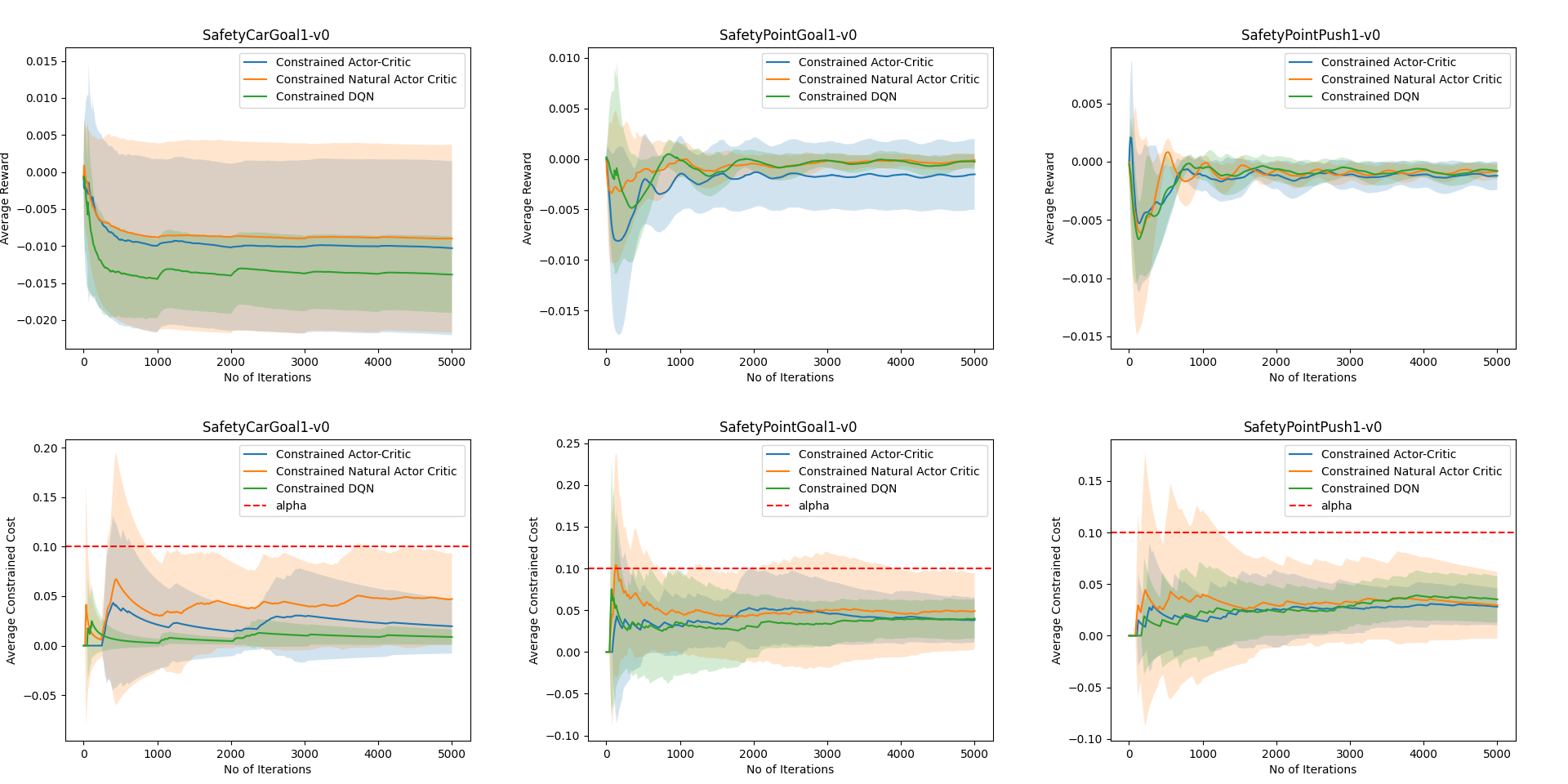
Figure 1: Comparison of C-AC , C-NAC and C-DQN: Plots in the top row are for the average reward performance while those in the bottom row are for the constraint costs for the three environments. These are plotted as functions of the number of iterations.

4.2.2 Convergence of the critic recursion for Algorithm 1

For the critic recursion, we obtain the following result for the average estimation error.

Theorem 2

We have

$$\frac{1}{1+t-\tau_{t}}\sum_{k=\tau_{t}}^{t}\mathbb{E}\|v_{k}-v^{*}(\theta_{k},\gamma(k))\|^{2}$$

$$=\mathcal{O}\bigg{(}\frac{1}{t^{1-\omega}}\bigg{)}+\mathcal{O}\bigg{(}\frac{\log t}{t^{\omega}}\bigg{)}+\mathcal{O}\bigg{(}\frac{1}{t^{2(\sigma-\omega)}}\bigg{)},$$ (7)

$$\frac{1}{1+t-\tau_{t}}\sum_{k=\tau_{t}}^{t}\mathbb{E}\big{(}L_{k}-L(\bm{\theta}_{k},\bm{\gamma}(k))\big{)}^{2}$$

$$=\mathcal{O}\bigg{(}\frac{1}{t^{1-\omega}}\bigg{)}+\mathcal{O}\bigg{(}\frac{\log t}{t^{\omega}}\bigg{)}+\mathcal{O}\bigg{(}\frac{1}{t^{2(\sigma-\omega)}}\bigg{)}.$$ (8)

4.2.3 Convergence rate and sample complexity for Algorithm 1

We finally provide the convergence rate of the algorithm and characterize the sample complexity of the same in Corollary 1.

Corollary 1

We have,

$$\min_{0\leq k\leq t}\mathbb{E}\|\nabla_{\bm{\theta}}L(\bm{\theta}_{k},\bm{\gamma}(k))\|^{2}=\mathcal{O}(\epsilon_{\text{app}})+\mathcal{O}\bigg{(}\frac{1}{t^{\beta-\sigma}}\bigg{)}$$

$$+\mathcal{O}\bigg{(}\frac{\log^{2}t}{t^{\omega}}\bigg{)}+\mathcal{O}\bigg{(}\frac{1}{t^{2(\sigma-\omega)}}\bigg{)}.$$

If we set $\omega=0.4,\sigma=0.6,\beta=1$, Algorithm 1 needs $T=\tilde{\mathcal{O}}(\epsilon^{-2.5})$ steps to obtain the following:

$$\min_{0\leq k\leq T}\mathbb{E}\big{\|}\nabla_{\bm{\theta}}L(\bm{\theta}_{k},\gamma(k))\big{\|}^{2} \leq\mathcal{O}(\epsilon_{\text{app}})+\epsilon.$$

Remark 1

In Corollary 1, the results of Theorems 1 and 2 are combined which results in the convergence rate of Algorithm 1 as $\tilde{\mathcal{O}}(t^{-0.4})$. The sample complexity of the constrained actor-critic algorithm is $\tilde{\mathcal{O}}(\epsilon^{-2.5})$ as we have exactly one sample per iteration.

4.3 Theoretical Results for Algorithm 2

As with Algorithm 1, we provide here the non-asymptotic convergence results for both the actor and the critic recursions in Algorithm 2. Further, we present the convergence rate and sample complexity of the algorithm.

4.3.1 Convergence of the Actor for Algorithm 2

We have the following result after carrying out non-asymptotic analysis of the actor.

Theorem 3

At the $t$-th iteration we have,

$$\min_{0\leq m\leq t}\mathbb{E}\big{\|}\nabla_{\bm{\theta}}L(\bm{\theta}_{m},\bm{\gamma}(m))\big{\|}^{2}$$

$$\qquad=\mathcal{O}(\epsilon_{\text{app}})+\mathcal{O}\big{(}t^{\sigma-\beta}\big{)}$$

$$\qquad+\mathcal{O}\bigg{(}\frac{\log^{2}t}{t^{\omega}}\bigg{)}+\mathcal{O}\bigg{(}\frac{\sum_{k=\tau_{t}}^{t}E\|A_{k}\|^{2}}{1+t-\tau_{t}}\bigg{)}$$

$$\qquad+\mathcal{O}\bigg{(}\frac{\sum_{k=\tau_{t}}^{t}E\|B_{k}\|^{2}}{1+t-\tau_{t}}\bigg{)},$$

where

$$A_{k} =L_{k}-L(\bm{\theta}_{k},\bm{\gamma}(k)),$$ (9)

$$B_{k} =v_{k}-v^{*}(\bm{\theta}_{k},\bm{\gamma}(k)).$$ (10)

Table 1: Comparision of C-AC , C-NAC and C-DQN in terms of average reward $\pm$ standard error upon convergence.

Algorithm	SafetyPointGoal1-v0	SafetyCarGoal1-v0	SafetyPointPush1-v0
C-AC	$-0.0015\pm 0.0035$	$-0.01\pm 0.0117$	$-0.0012\pm 0.0011$
C-NAC	$-0.00012\pm 0.0006$	$-0.009\pm 0.0127$	$-0.0008\pm 0.0005$
C-DQN	$-0.0003\pm 0.0007$	$-0.014\pm 0.005$	$-0.0008\pm 0.0007$

4.3.2 Convergence of the Critic for Algorithm 2

We now provide a result analysing the average estimation error for the critic.

Theorem 4

We have the following:

$$\frac{1}{1+t-\tau_{t}}\sum_{k=\tau_{t}}^{t}\mathbb{E}\|v_{k}-v^{*}(\bm{\theta}_{k},\bm{\gamma}(k))\|^{2}$$

$$=\mathcal{O}\bigg{(}\frac{1}{t^{1-\omega}}\bigg{)}+\mathcal{O}\bigg{(}\frac{\log t}{t^{\omega}}\bigg{)}+\mathcal{O}\bigg{(}\frac{1}{t^{2(\sigma-\omega)}}\bigg{)},$$ (11)

$$\frac{1}{1+t-\tau_{t}}\sum_{k=\tau_{t}}^{t}\mathbb{E}\big{(}L_{k}-L(\bm{\theta}_{k},\bm{\gamma}(k))\big{)}^{2}$$

$$=\mathcal{O}\bigg{(}\frac{1}{t^{1-\omega}}\bigg{)}+\mathcal{O}\bigg{(}\frac{\log t}{t^{\omega}}\bigg{)}+\mathcal{O}\bigg{(}\frac{1}{t^{2(\sigma-\omega)}}\bigg{)}.$$ (12)

4.3.3 Convergence rate and sample complexity for Algorithm 2

We finally provide the convergence rate of the algorithm and characterize the sample complexity of the same in Corollary 2.

Corollary 2

We have

$$\min_{0\leq k\leq t}\mathbb{E}\|\nabla_{\bm{\theta}}L(\bm{\theta}_{k},\bm{\gamma}(k))\|^{2}=\mathcal{O}(\epsilon_{\text{app}})+\mathcal{O}\bigg{(}\frac{1}{t^{\beta-\sigma}}\bigg{)}$$

$$+\mathcal{O}\bigg{(}\frac{\log^{2}t}{t^{\omega}}\bigg{)}+\mathcal{O}\bigg{(}\frac{1}{t^{2(\sigma-\omega)}}\bigg{)}.$$

If we set $\omega=0.4,\sigma=0.6,\beta=1$, Algorithm 2 needs $T=\tilde{\mathcal{O}}(\epsilon^{-2.5})$ steps to obtain the following,

$$\min_{0\leq k\leq T}\mathbb{E}\big{\|}\nabla_{\bm{\theta}}L(\bm{\theta}_{k},\gamma(k))\big{\|}^{2} \leq\mathcal{O}(\epsilon_{\text{app}})+\epsilon,$$

4.4 Proof Sketch for Theorems 1 and 3

We provide here an overview of the manner in which the proofs of Theorems 1 and 3 proceed. This also helps us to describe the connection between the various results mentioned above. The proofs of Theorems 1 and 3 rely crucially on Lemma D.6 below.

Lemma 1

For all $\bm{\gamma}\in R^{N}$ with $0\leq\bm{\gamma}_{i}\leq M$ where $i\in\{1,2,...,N\}$, there exists a constant $M_{L}$ greater than 0 such that for all $\theta_{1},\theta_{2}\in{R^{d}}$,

$$\|\nabla_{\theta}L(\theta_{1},\bm{\gamma})-\nabla_{\theta}L(\theta_{2},\bm{\gamma})\|\leq M_{L}\|\theta_{1}-\theta_{2}\|.$$

As a result of this lemma, we have the following inequality (see Wu et al., [2020], Lemma C.1) $\forall t>0$ that we use in the proof of Theorem 1.

$$L(\theta_{t+1},\bm{\gamma}(t))\geq L(\theta_{t},\bm{\gamma}(t))$$

$$+b(t)\langle\nabla_{\theta}L(\theta_{t},\bm{\gamma}(t)),\delta_{t}\nabla\log\pi_{\theta_{t}}(a_{t}|s_{t})\rangle$$

$$-\frac{M_{L}}{2}b(t)^{2}\|\delta_{t}\nabla\log\pi_{\theta_{t}}(a_{t}|s_{t})\|^{2}.$$ (13)

The key idea in the proof (see Appendix for details) is to split the middle term in the RHS of (13) into a few terms, of which one is $b(t)\|\nabla L(\bm{\theta}_{t},\bm{\gamma}(t))\|^{2}$. We obtain an upper bound for $\|\nabla L(\bm{\theta}_{t},\bm{\gamma}(t))\|^{2}$. After summing the expectation of terms on both sides, we analyse each term in the bound to get the desired result for Theorem 1. Note also that the result for Theorem 1 depends on the convergence of the critic parameter and the average cost estimator. So we find a bound on the averaged estimation errors by the critic and average cost estimator in Theorem 2. We then get an inequality similar to (13) for Theorem 3 (see Appendix) and carry out an analysis along similar lines for Theorems 3 and 4.

Remark 2

Analogous to Remark 1, in Corollary 2, the results of Theorems 3 and 4 are combined which gives the convergence rate of (natural actor critic) Algorithm 2 as $\tilde{\mathcal{O}}(t^{-0.4})$ and a sample complexity of $\tilde{\mathcal{O}}(\epsilon^{-2.5})$ as we have one per-iteration sample in this algorithm as well. It is important to also mention that for the results of both algorithms, $\mathcal{O}(\cdot)$ hides the terms that do not depend on the iteration number.

5 Experimental Results

In this section we present the results of our experiments on three different settings: (a) the OpenAI Safety-Gym environment - SafetyPointGoal1-v0, (b) the OpenAI Safety-Gym environment SafetyCarGoal1-v0 and (c) the OpenAI Safety-Gym environment SafetyPointPush1-v0. The performance comparisons on these environments can be seen in Figure 1 and Tables 1 and 2, respectively. The two tables summarize the performance obtained upon convergence of the algorithms. Note that Table 2 has been placed in the appendix for lack of space. We also explain the Constrained DQN algorithm that we implemented in the appendix.

All the plots of our experiments are obtained after averaging over 10 different initial seeds. The performance of the algorithms is compared by plotting the average reward along with standard errors. The dotted flat red-line in each of the plots in the lower row of plots in Figure 1 corresponds to the constraint cost threshold. All algorithms are seen to asymptotically satisfy the constraint threshold while optimizing on the average reward performance.

It can be observed that our C-NAC algorithm performs better than the other two algorithms on all three settings and C-AC shows the second best results on two of the three environments. Moreover, the cost threshold is met by all the three algorithms.

6 Conclusions

We presented the first (non-asymptotic) finite time convergence analysis of constrained actor critic and constrained natural actor critic algorithms using linear function approximation and obtained a sample complexity of $\mathcal{\tilde{O}}(\epsilon^{-2.5})$ for both (three timescale) algorithms. Our sample complexity result is significant as for both our algorithms it matches the sample complexity of regular (unconstrained) actor critic (two timescale) algorithms (cf. Wu et al., [2020]). We also showed the results of experiments on three different Safety-Gym environments, where we observed that the C-NAC algorithm is better than both the C-AC and the C-DQN algorithms in the average reward performance and the C-AC algorithm is the second best performer on two of these three settings. Further, the average cost constraint is met by all the three algorithms on each of the settings.

Appendix

Appendix A Preliminaries

For our problem, we have considered random single-stage costs and also constraint costs having distributions that are dependent on the current state, action and next state. For a given tuple $O_{t}=(s_{t},a_{t},s_{t+1})$, we consider

$$q(t)\sim\bar{p}(.|s_{t},a_{t},s_{t+1}),\mbox{ }h_{i}(t)\sim p_{i}(.|s_{t},a_{t},s_{t+1}),$$

for $i=1,2,3,..,N$. For a given $\gamma=(\gamma_{1},\gamma_{2},...,\gamma_{N})^{T}$ with $0\leq\gamma_{i}\leq M$ and for $i=1,2,..,N$, we define $c(t)=q(t)+\sum\limits_{k=1}^{N}\gamma_{k}(h_{k}(t)-\alpha_{k})$ such that

$$c(t)\sim\hat{p}(.|s_{t},a_{t},s_{t+1}).$$

Since the single stage costs are mutually independent for any state-action-next state tuple, we have

$$\hat{p}(c(t)|s_{t},a_{t},s_{t+1})=\bar{p}(q(t)|s_{t},a_{t},s_{t+1})\prod\limits_{i=1}^{N}p_{i}(h_{i}(t)|s_{t},a_{t},s_{t+1}).$$

Let $\|\nabla L(\theta,\gamma)\|<U_{L},\forall\theta,\gamma$ where $U_{L}>0$ is a positive constant. Also, $\sup\limits_{t}\|G(t)^{-1}\|\leq U_{G}$ where $U_{G}$ is a positive constant.Recall that the single stage costs $q(n),h_{1}(n),\ldots,h_{N}(n)$ are non-negative and absolutely bounded by a constant $U_{c}>0$.We define $U_{r}=U_{c}+NM(U_{c}+U_{\alpha})$ where $U_{\alpha}=\max\limits_{k}|\alpha_{k}|$. We assume $0\leq L_{0}\leq U_{r}$. This implies $|L_{t}|\leq U_{r},\forall t>0$. We also assume $0\leq U_{k}(0)\leq U_{c},\forall k\in{1,2,..,N}$, which implies $|U_{k}(t)|\leq U_{c},\forall t>0$. Moreover, we assume that the projection set $C$ to which the recursion $v_{t}$ is projected is a compact and convex set.

Given time indices $t$ and $\tau$ such that $t\geq\tau>0$, we consider the following auxiliary Markov chain starting from $s_{t-\tau}$ to deal with Markov noise in the iterates.

$$s_{t-\tau}\xrightarrow{\theta_{t-\tau}}a_{t-\tau}\xrightarrow{\mathcal{P}}s_{t-\tau+1}\xrightarrow{\theta_{t-\tau}}\widetilde{a}_{t-\tau+1}\xrightarrow{\mathcal{P}}\widetilde{s}_{t-\tau+2}\xrightarrow{\theta_{t-\tau}}\widetilde{a}_{t-\tau+2}\cdots\xrightarrow{\mathcal{P}}\widetilde{s}_{t}\xrightarrow{\theta_{t-\tau}}\widetilde{a}_{t}\xrightarrow{\mathcal{P}}\widetilde{s}_{t+1}.$$ (14)

The original Markov chain has the following transitions:

$$s_{t-\tau}\xrightarrow{\theta_{t-\tau}}a_{t-\tau}\xrightarrow{\mathcal{P}}s_{t-\tau+1}\xrightarrow{\theta_{t-\tau+1}}a_{t-\tau+1}\xrightarrow{\mathcal{P}}s_{t-\tau+2}\xrightarrow{\theta_{t-\tau+2}}a_{t-\tau+2}\cdots\xrightarrow{\mathcal{P}}s_{t}\xrightarrow{\theta_{t}}a_{t}\xrightarrow{\mathcal{P}}s_{t+1}.$$ (15)

In (14), for any time instant $k>t-\tau$, $\widetilde{a}_{k}$ denotes the action taken in the auxiliary Markov chain. Similarly, for any time instant $l>t-\tau+1$, $\widetilde{s}_{l}$ denotes the state in the auxiliary Markov chain. In the following, without any other specification, $E[.]$ will denote the expectation w.r.t the joint distribution of all the random variables involved. Finally, we mention that for our analysis we interchangeably use $\pi(a|s)$ and $\pi(s,a)$ to mean the action chosen in state $s$ according to the policy $\pi$. Thus, both these notations are one and the same.

Appendix B Proof of Proposition 1

Proof B.5.

Let

$$\mathbf{A}_{\bm{\theta}} :=\mathbb{E}_{s_{n},a_{n},s_{n+1}}\big{[}f_{s_{n}}\big{(}f_{s_{n+1}}-f_{s_{n}}\big{)}^{\top}\big{]},$$

$$\mathbf{b}_{\bm{\theta},\bm{\gamma}} :=\mathbb{E}_{s_{n},a_{n},s_{n+1}}[(C(s_{n},a_{n},\gamma)-L(\bm{\theta},\gamma))f_{s_{n}}],$$

where $s_{n}\sim\mu_{\bm{\theta}}(\cdot),a_{n}\sim\pi_{\bm{\theta}}(\cdot|s),s_{n+1}\sim p(s_{n},\cdot,a_{n})$ .

From section 4.1 of the main paper ,we have,

$$\mathbf{A}_{\theta}v^{*}(\theta,\gamma)+\mathbf{b}_{\theta,\gamma} =\mathbf{0}.$$

Thus,

$$\big{\|}v^{*}(\theta_{1},\bm{\gamma})-v^{*}(\theta_{2},\bm{\gamma})\big{\|} =\|\mathbf{A}_{\theta_{1}}^{-1}\mathbf{b}_{\theta_{1},\gamma}-\mathbf{A}_{\theta_{2}}^{-1}\mathbf{b}_{\theta_{2},\gamma}\|$$

$$\leq\|\mathbf{A}_{\theta_{1}}^{-1}\mathbf{b}_{\theta_{1},\gamma}-\mathbf{A}_{\theta_{2}}^{-1}\mathbf{b}_{\theta_{1},\gamma}\|+\|\mathbf{A}_{\theta_{2}}^{-1}\mathbf{b}_{\theta_{1},\gamma}-\mathbf{A}_{\theta_{2}}^{-1}\mathbf{b}_{\theta_{2},\gamma}\|$$

$$\leq\|\mathbf{A}_{\theta_{1}}^{-1}-\mathbf{A}_{\theta_{2}}^{-1}\|\|\mathbf{b}_{\theta_{1},\gamma}\|+\|\mathbf{A}_{\theta_{2}}^{-1}\|\|\mathbf{b}_{\theta_{1},\gamma}-\mathbf{b}_{\theta_{2},\gamma}\|.$$

It can be shown that

$$\|\mathbf{b}_{\theta_{1},\gamma}\| \leq 2U_{r},$$

$$\|\mathbf{A}_{\theta_{2}}^{-1}\| \leq\lambda_{e}^{-1},$$

$$\mathbf{A}_{\theta_{1}}^{-1}-\mathbf{A}_{\theta_{2}}^{-1} =\mathbf{A}_{\theta_{1}}^{-1}(\mathbf{A}_{\theta_{2}}-\mathbf{A}_{\theta_{1}})\mathbf{A}_{\theta_{2}}^{-1},$$

We have from section B.2 of Wu et al., [2020] the following:

$$\|\mathbf{A}_{\theta_{1}}-\mathbf{A}_{\theta_{2}}\| \leq 4|A|L\bigg{(}1+\lceil\log_{k}b^{-1}\rceil+\frac{1}{1-k}\bigg{)}\|\bm{\theta}_{1}-\bm{\theta}_{2}\|,$$

$$\|\mathbf{b}_{\theta_{1},\gamma}-\mathbf{b}_{\theta_{2},\gamma}\| \leq 6|A|U_{r}L\bigg{(}1+\lceil\log_{k}b^{-1}\rceil+\frac{1}{1-k}\bigg{)}\|\bm{\theta}_{1}-\bm{\theta}_{2}\|.$$

After combining all the terms, we have

$$\big{\|}v^{*}(\bm{\theta}_{1},\bm{\gamma})-v^{*}(\bm{\theta}_{2},\bm{\gamma})\big{\|}\leq L_{1}\|\bm{\theta}_{1}-\bm{\theta}_{2}\|,\forall\bm{\theta}_{1},\bm{\theta}_{2}\in\mathbb{R}^{d},$$

where $L_{1}=(8\lambda_{e}^{-2}+6\lambda_{e}^{-1})U_{r}|A|L\bigg{(}1+\lceil\log_{k}b^{-1}\rceil+\frac{1}{1-k}\bigg{)}$.

Appendix C Proof of Proposition 2

We have,

$$\big{\|}v^{*}(\theta,\bm{\gamma}^{1})-v^{*}(\theta,\bm{\gamma}^{2})\big{\|} =\|\mathbf{A}_{\theta}^{-1}\mathbf{b}_{\theta,\bm{\gamma}^{1}}-\mathbf{A}_{\theta}^{-1}\mathbf{b}_{\theta,\bm{\gamma}^{2}}\|$$

$$\leq\|\mathbf{A}_{\theta}^{-1}\|\underbrace{\|\mathbf{b}_{\theta,\bm{\gamma}^{1}}-\mathbf{b}_{\theta,\bm{\gamma}^{2}}\|}_{I_{1}}.$$

Now for the term $I_{1}$, note that

$$\|\mathbf{b}_{\theta,\bm{\gamma}^{1}}-\mathbf{b}_{\theta,\bm{\gamma}^{2}}\| =\|E_{\{s_{n}\sim\mu_{\bm{\theta}}(\cdot),a_{n}\sim\pi_{\bm{\theta}}(\cdot|s),s_{n+1}\sim p(s_{n},\cdot,a_{n})\}}[(C(s_{n},a_{n},\bm{\gamma}^{1})-C(s_{n},a_{n},\bm{\gamma}^{2})+L(\bm{\theta},\bm{\gamma}^{2})-L(\bm{\theta},\bm{\gamma}^{1}))f_{s_{n}}]\|$$

$$\leq 2N(U_{c}+U_{\alpha})|\bm{\gamma}_{p}^{1}-\bm{\gamma}_{p}^{2}|,$$

where, $|\bm{\gamma}_{p}^{1}-\bm{\gamma}_{p}^{2}|=\max\limits_{i=1,2,...,N}|\bm{\gamma}_{i}^{1}-\bm{\gamma}_{i}^{2}|$. Hence,

$$\big{\|}v^{*}(\bm{\theta},\bm{\gamma}^{1})-v^{*}(\bm{\theta},\bm{\gamma}^{2})\big{\|}\leq L_{2}|\bm{\gamma}_{p}^{1}-\bm{\gamma}_{p}^{2}|,\forall\bm{\gamma}_{1},\bm{\gamma}_{2}\in\mathbb{R}^{N},$$

where, $L_{2}=(2N(U_{c}+U_{\alpha}))/\lambda_{e}$.

Appendix D Proof of Theorems

D.1 Proof of Theorem 1

We first define several notations to clarify the dependence in the various quantities involved. Let

$$\begin{split}O_{t}:&=(s_{t},a_{t},s_{t+1}),\\ L^{*}:&=L(\theta,\gamma)=E_{s\sim\mu_{\theta},a\sim\pi_{\theta}}[d(s,a)+\sum_{k=1}^{N}\gamma(k)(h_{k}(s,a)-\alpha_{k})],\\ v(k)^{*}:&=v^{*}(\theta_{k},\gamma(k)),\\ \Delta H(O,L,v,\theta,\gamma):&=(L(\theta,\gamma)-L+({f_{s^{{}^{\prime}}}}^{T}-f_{s}^{T})(v-v^{*}(\theta,\gamma)))\nabla\log\pi_{\theta}(a|s),\\ H(O,\theta,\gamma,q,h):&=(q-L(\theta,\gamma)+\sum_{k=1}^{N}\gamma(k)(h_{k}-\alpha_{k})+({f_{s^{{}^{\prime}}}}^{T}-f_{s}^{T})v^{*}(\theta,\gamma))\nabla\log\pi_{\theta}(a|s),\\ \Delta H^{{}^{\prime}}(O,\theta,\gamma):&=({f_{s^{{}^{\prime}}}}^{T}v^{*}(\theta,\gamma)-V^{\theta,\gamma}(s^{{}^{\prime}})-({f_{s}}^{T}v^{*}(\theta,\gamma)-V^{\theta,\gamma}(s)))\nabla\log\pi_{\theta}(a|s),\\ \check{\Gamma}(O,\theta,\gamma,q,h):&=\langle\nabla L(\theta,\gamma),H(O,\theta,\gamma,q,h)-E_{O^{{}^{\prime}},q,h}[H(O^{{}^{\prime}},\theta,\gamma,q,h)]\rangle.\\ \end{split}$$ (16)

In the above, $O=(s,a,s^{{}^{\prime}})$, $h=(h_{1},h_{2},h_{3},...,h_{N})$.$O^{{}^{\prime}}=(s,a,s^{{}^{\prime}})$ denotes the independent sample $s\sim\mu_{\theta},$ $a\sim\pi_{\theta}$, $s^{{}^{\prime}}\sim p(s,.,a)$ .Hence $E_{O^{{}^{\prime}},q,h}[\cdot]$ denotes expectation w.r.t. the joint distribution of $s\sim\mu_{\theta},$ $a\sim\pi_{\theta}$, $s^{{}^{\prime}}\sim p(s,.,a)$, $q\sim\bar{p}(.|s,a,s^{{}^{\prime}})$, $h_{i}\sim p_{i}(.|s,a,s^{{}^{\prime}})$, $i=1,\ldots,N$. We now have,

$$E_{O^{{}^{\prime}},q,h}[(H(O^{{}^{\prime}},\theta,\gamma,q,h)-\Delta H^{{}^{\prime}}(O^{{}^{\prime}},\theta,\gamma)]$$

$$=E_{O^{{}^{\prime}},q,h}[q+\sum_{k=1}^{N}\gamma(k)(h_{k}-\alpha_{k})-L(\theta,\gamma)+V^{\theta,\gamma}(s^{{}^{\prime}})-V^{\theta,\gamma}(s))\nabla\log\pi_{\theta}(a|s)]$$

$$=\nabla L(\theta,\gamma),$$

Next, observe that

$$E_{O^{{}^{\prime}}}\|\Delta H^{{}^{\prime}}(O,\theta,\gamma)\|^{2} =E_{O^{{}^{\prime}}}\|({f_{s^{{}^{\prime}}}}^{T}v^{*}(\theta,\gamma)-V^{\theta,\gamma}(s^{{}^{\prime}})-({f_{s}}^{T}v^{*}(\theta,\gamma)-V^{\theta,\gamma}(s)))\nabla\log\pi_{\theta}(a|s)\|^{2}$$

$$\leq E_{O^{{}^{\prime}}}[D^{2}({f_{s^{{}^{\prime}}}}^{T}v^{*}(\theta,\gamma)-V^{\theta,\gamma}(s^{{}^{\prime}})-({f_{s}}^{T}v^{*}(\theta,\gamma)-V^{\theta,\gamma}(s)))^{2}]$$

$$\leq E_{O^{{}^{\prime}}}[2D^{2}(({f_{s^{{}^{\prime}}}}^{T}v^{*}(\theta,\gamma)-V^{\theta,\gamma}(s^{{}^{\prime}}))^{2}+({f_{s}}^{T}v^{*}(\theta,\gamma)-V^{\theta,\gamma}(s))^{2})]$$

$$\leq 4D^{2}\epsilon_{app}^{2}.$$

Before we proceed further, we first state and prove Lemmas 1–4 below that will be used in the proof of Theorem 1. Moreover, the proof of Lemma 4 shall rely on Lemmas D.13.1 – D.13.4 that we also state and prove in the following. Finally, collecting all these results together, we shall obtain the claim for Theorem 1.

Lemma D.6.

For all $\bm{\gamma}\in R^{N}$, with $0\leq\bm{\gamma}_{i}\leq M$, where $i\in\{1,2,...,N\}$, there exists a constant $M_{L}$ greater than 0 such that for all $\theta_{1},\theta_{2}\in{R^{d}}$,

$$\|\nabla L(\theta_{1},\bm{\gamma})-\nabla L(\theta_{2},\bm{\gamma})\|\leq M_{L}\|\theta_{1}-\theta_{2}\|,$$

which implies

$$L(\theta_{2},\gamma)>L(\theta_{1},\gamma)+\langle\nabla L(\theta_{1},\gamma),\theta_{2}-\theta_{1}\rangle-\frac{M_{L}}{2}\|\theta_{1}-\theta_{2}\|^{2}.$$

Proof D.7.

Note that

$$L(\theta,\gamma)=J(\theta)+\sum\limits_{k=1}^{N}\gamma(k)(G_{k}(\theta)-\alpha_{k}).$$

$$\Rightarrow\nabla_{\theta}L(\theta,\gamma)=\nabla_{\theta}J(\theta)+\sum\limits_{k=1}^{N}\gamma(k)\nabla_{\theta}G_{k}(\theta).$$

From Lemma C.1 of Wu et al., [2020], we have $\forall\theta_{1},\theta_{2}\in R^{d}$, there exist positive constants $L_{J},L_{G_{1}},L_{G_{2}},...,L_{G_{N}}$ such that

$$\|\nabla_{\theta}J(\theta_{1})-\nabla_{\theta}J(\theta_{2})\| \leq L_{J}\|\theta_{1}-\theta_{2}\|,$$

$$\|\nabla_{\theta}G_{i}(\theta_{1})-\nabla_{\theta}G_{i}(\theta_{2})\| \leq L_{G_{i}}\|\theta_{1}-\theta_{2}\|,\forall i\in{1,2,..,N}.$$

Hence,

$$\|\nabla_{\theta}L(\theta_{1},\gamma)-\nabla_{\theta}L(\theta_{2},\gamma)\| =\|\nabla_{\theta}J(\theta_{1})-\nabla_{\theta}J(\theta_{2})+\sum\limits_{k=1}^{N}\gamma_{k}(\nabla_{\theta}G_{k}(\theta_{1})-\nabla_{\theta}G_{k}(\theta_{2}))\|$$

$$\leq\|\nabla_{\theta}J(\theta_{1})-\nabla_{\theta}J(\theta_{2})\|+\sum\limits_{k=1}^{N}\gamma_{k}\|\nabla_{\theta}G_{k}(\theta_{1})-\nabla_{\theta}G_{k}(\theta_{2})\|$$

$$\leq L_{J}\|\theta_{1}-\theta_{2}\|+\sum\limits_{k=1}^{N}\gamma_{k}L_{G_{k}}\|\theta_{1}-\theta_{2}\|$$

$$=(L_{J}+\sum\limits_{k=1}^{N}\gamma_{k}L_{G_{k}})\|\theta_{1}-\theta_{2}\|$$

$$\leq M_{L}\|\theta_{1}-\theta_{2}\|.$$

So we have,

$$\|\nabla_{\theta}L(\theta_{1},\gamma)-\nabla_{\theta}L(\theta_{2},\gamma)\|\leq M_{L}\|\theta_{1}-\theta_{2}\|,\forall\theta_{1},\theta_{2}\in R^{d},$$

where $M_{L}=L_{J}+M\sum\limits_{k=1}^{N}L_{G_{k}}$. The claim follows.

Lemma D.8.

For all $\bm{\gamma}^{1},\bm{\gamma}^{2}\in R^{N}$ with $0\leq\bm{\gamma}_{i}^{j}\leq M$, where $i\in\{1,2,...,N\}$, $j=1,2$, there exists a constant $C$ greater than 0 such that for all $\bm{\theta}\in{R^{d}}$,

$$\|\nabla L(\bm{\theta},\bm{\gamma}^{1})-\nabla L(\bm{\theta},\bm{\gamma}^{2})\|\leq C|\bm{\gamma}^{1}_{m}-\bm{\gamma}^{2}_{m}|,\$$

where $|\bm{\gamma}^{1}_{m}-\bm{\gamma}^{2}_{m}|=\max\limits_{i=1,2,..,N}|\bm{\gamma}^{1}_{i}-\bm{\gamma}^{2}_{i}|$.

Proof D.9.

We have,

$$\|\nabla L(\bm{\theta},\bm{\gamma}^{1})-\nabla L(\bm{\theta},\bm{\gamma}^{2})\| =\bigg{\|}\sum\limits_{s\in S}\mu_{\bm{\theta}}(s)\sum\limits_{a\in A(s)}\pi_{\bm{\theta}}(a|s)(M^{\pi_{\bm{\theta}},\bm{\gamma}^{1}}(s,a)-M^{\pi_{\bm{\theta}},\bm{\gamma}^{2}}(s,a))\nabla\log\pi_{\bm{\theta}}(a|s)\bigg{\|}$$

$$\leq\sum\limits_{s\in S}\mu_{\bm{\theta}}(s)\sum\limits_{a\in A(s)}\pi_{\bm{\theta}}(a|s)\big{\|}(M^{\pi_{\bm{\theta}},\bm{\gamma}^{1}}(s,a)-M^{\pi_{\bm{\theta}},\bm{\gamma}^{2}}(s,a))\nabla\log\pi_{\bm{\theta}}(a|s)\big{\|}$$

$$\leq D\sum\limits_{s\in S}\mu_{\bm{\theta}}(s)\sum\limits_{a\in A(s)}\pi_{\bm{\theta}}(a|s)\big{|}M^{\pi_{\bm{\theta}},\bm{\gamma}^{1}}(s,a)-M^{\pi_{\bm{\theta}},\bm{\gamma}^{2}}(s,a)\big{|},$$

where the last inequality follows from Assumption 4. Now,

$$\big{|}M^{\pi_{\bm{\theta}},\bm{\gamma}^{1}}(s,a)-M^{\pi_{\bm{\theta}},\bm{\gamma}^{2}}(s,a))\big{|} =\big{|}\sum\limits_{t=1}^{\infty}E\bigg{[}\sum\limits_{i=1}^{N}(\bm{\gamma}^{1}_{i}-\bm{\gamma}^{2}_{i})(h_{i}(t)-G_{i}(\bm{\theta}))|s_{0}=s,a_{0}=a,\pi_{\bm{\theta}}\bigg{]}\big{|}$$

$$=\bigg{|}\sum\limits_{i=1}^{N}(\bm{\gamma}^{1}_{i}-\bm{\gamma}^{2}_{i})\sum\limits_{t=1}^{\infty}E\bigg{[}(h_{i}(t)-G_{i}(\bm{\theta}))|s_{0}=s,a_{0}=a,\pi_{\theta}\bigg{]}\bigg{|}$$

$$\leq\sum\limits_{i=1}^{N}|(\bm{\gamma}^{1}_{i}-\bm{\gamma}^{2}_{i})|\bigg{|}\sum\limits_{t=1}^{\infty}E\bigg{[}(h_{i}(t)-G_{i}(\bm{\theta}))|s_{0}=s,a_{0}=a,\pi_{\theta}\bigg{]}\bigg{|}$$

$$\leq N\bar{Q}|\bm{\gamma}^{1}_{m}-\bm{\gamma}^{2}_{m}|,$$

where,

$$\bar{Q} =\sup\limits_{i,\bm{\theta},s,a}|Q^{\bm{\theta}}_{i}(s,a)|,$$

$$|\bm{\gamma}^{1}_{m}-\bm{\gamma}^{2}_{m}| =\max_{i=1,2,..,N}|\bm{\gamma}^{1}_{i}-\bm{\gamma}^{2}_{i}|,$$

and where $Q^{\bm{\theta}}_{i}(s,a)$ is the expected differential cost for the state action pair $(s,a)$ with single-stage cost as $h_{i}(t)$ at time instant $t$ when actions are picked according to policy $\pi_{\bm{\theta}}$. Hence,

$$\|\nabla L(\bm{\theta},\bm{\gamma}^{1})-\nabla L(\bm{\theta},\bm{\gamma}^{2})\|\leq ND\bar{Q}|\bm{\gamma}^{1}_{m}-\bm{\gamma}^{2}_{m}|.$$

The claim follows by letting $C=ND\bar{Q}$.

Lemma D.10.

For any $t>0$,

$$\|\Delta H(O_{t},L_{t},v_{t},\theta_{t},\gamma(t))\|^{2}\leq D^{2}(2(L_{t}-L(\theta_{t},\gamma(t)))^{2}+8\|v_{t}-v(t)^{*}\|^{2}).$$

Proof D.11.

Applying the definition of $\Delta H(\cdot)$ immediately yields the result.

Lemma D.12.

For any $t\geq 0$,

$$E[\check{\Gamma}(O_{t},\theta_{t},\gamma(t),q(t),h(t))]\geq-(D_{1}(\tau+1)\sum_{k=t-\tau+1}^{t}E\|\theta_{k}-\theta_{k-1}\|+D_{2}bk^{\tau-1}+T_{1}\sum_{i=t-\tau+1}^{t}E|\gamma_{m}(i)-\gamma_{m}(i-1)|),$$

where $D_{1},D_{2}$ and $T_{1}$ are positive constants and $t\geq\tau\geq 0$.

Proof D.13.

We have

$$E[\check{\Gamma}(O_{t},\theta_{t},\gamma(t),q(t),h(t))]$$

$$=E_{s_{t}\sim p,a_{t}\sim\pi_{\theta_{t}},s_{t+1}\sim p}[E[\langle\nabla L(\theta_{t},\gamma(t)),H(O_{t},\theta_{t},\gamma(t),q(t),h(t))-E_{O^{{}^{\prime}},q,h}[H(O^{{}^{\prime}},\theta_{t},\gamma(t),q,h)]\rangle|s_{t},a_{t},s_{t+1}]]$$

$$=E[\langle\nabla L(\theta_{t},\gamma(t)),\bar{H}(O_{t},\theta_{t},\gamma(t))-E_{O^{{}^{\prime}},q,h}[H(O^{{}^{\prime}},\theta_{t},\gamma(t),q,h)]\rangle]$$

$$=E[\langle\nabla L(\theta_{t},\gamma(t)),\bar{H}(O_{t},\theta_{t},\gamma(t))-E_{O^{{}^{\prime}}}[E_{q,h}[H(O^{{}^{\prime}},\theta_{t},\gamma(t),q,h)|s,a,s^{{}^{\prime}}]]\rangle]$$

$$=E[\langle\nabla L(\theta_{t},\gamma(t)),\bar{H}(O_{t},\theta_{t},\gamma(t))-E_{O^{{}^{\prime}}}[\bar{H}(O^{{}^{\prime}},\theta_{t},\gamma(t))]\rangle]$$

$$=E[Q(O_{t},\theta_{t},\gamma(t))],$$

where,

$$\bar{H}(O,\theta,\gamma) =(c(s,a,s^{{}^{\prime}},\gamma)-L(\theta,\gamma)+({f_{s^{{}^{\prime}}}}^{T}-{f_{s}}^{T})v^{*}(\theta,\gamma))\nabla\log\pi_{\theta}(a|s)$$

$$c(s,a,s^{{}^{\prime}},\gamma) =\sum\limits_{q}(q\cdot\bar{p}(q|s,a,s^{{}^{\prime}}))+\sum\limits_{k=1}^{k=N}\gamma_{k}(\sum\limits_{h}(h\cdot p_{k}(h|s,a,s^{{}^{\prime}}))-\alpha_{k}).$$

The second equality is satisfied because $\theta_{t}$ and $\gamma(t)$ do not depend on $q(t)$ and $h(t)$. The remaining proof of Lemma D.12 in turn requires Lemmas D.13.1 – D.13.4 below that we now state and prove.

lemma D.13.1

For any $t\geq 0$,

$$|Q(O_{t},\theta_{t},\gamma(t))-Q(O_{t},\theta_{t},\gamma(t-\tau))|\leq T_{1}|\gamma_{m}(t)-\gamma_{m}(t-\tau)|,$$

where $T_{1}>0$ is a constant.

Proof Denoting $O=(s,a,s^{{}^{\prime}})$, we have for any $\theta,\gamma_{1},\gamma_{2}$, that

$$Q(O,\theta,\gamma^{1})-Q(O,\theta,\gamma^{2})$$

$$=\langle\nabla L(\theta,\gamma^{1}),\bar{H}(O,\theta,\gamma^{1})-E_{O^{{}^{\prime}}}[\bar{H}(O^{{}^{\prime}},\theta,\gamma^{1})]\rangle-\langle\nabla L(\theta,\gamma^{2}),\bar{H}(O,\theta,\gamma^{2})-E_{O^{{}^{\prime}}}[\bar{H}(O^{{}^{\prime}},\theta,\gamma^{2})]\rangle$$

$$=\langle\nabla L(\theta,\gamma^{1}),\bar{H}(O,\theta,\gamma^{1})-E_{O^{{}^{\prime}}}[\bar{H}(O^{{}^{\prime}},\theta,\gamma^{1})]\rangle-\langle\nabla L(\theta,\gamma^{1}),\bar{H}(O,\theta,\gamma^{2})-E_{O^{{}^{\prime}}}[\bar{H}(O^{{}^{\prime}},\theta,\gamma^{2})]\rangle$$

$$\qquad+\langle\nabla L(\theta,\gamma^{1}),\bar{H}(O,\theta,\gamma^{2})-E_{O^{{}^{\prime}}}[\bar{H}(O^{{}^{\prime}},\theta,\gamma^{2})]\rangle-\langle\nabla L(\theta,\gamma^{2}),\bar{H}(O,\theta,\gamma^{2})-E_{O^{{}^{\prime}}}[\bar{H}(O^{{}^{\prime}},\theta,\gamma^{2})]\rangle$$

$$=\underbrace{\langle\nabla L(\theta,\gamma^{1}),\bar{H}(O,\theta,\gamma^{1})-\bar{H}(O,\theta,\gamma^{2})-E_{O^{{}^{\prime}}}[\bar{H}(O^{{}^{\prime}},\theta,\gamma^{1})]+E_{O^{{}^{\prime}}}[\bar{H}(O^{{}^{\prime}},\theta,\gamma^{2})]\rangle}_{I_{1}}$$

$$\qquad+\underbrace{\langle\nabla L(\theta,\gamma^{1})-\nabla L(\theta,\gamma^{2}),\bar{H}(O,\theta,\gamma^{2})-E_{O^{{}^{\prime}}}[\bar{H}(O^{{}^{\prime}},\theta,\gamma^{2})]\rangle}_{I_{2}}.$$

Now,

$$\|\bar{H}(O,\theta,\gamma^{1})-\bar{H}(O,\theta,\gamma^{2})\|$$

$$=\|(c(s,a,s^{{}^{\prime}},\gamma^{1})-c(s,a,s^{{}^{\prime}},\gamma^{2})-L(\theta,\gamma^{1})+L(\theta,\gamma^{2})+({f_{s^{{}^{\prime}}}}^{T}-{f_{s}}^{T})(v^{*}(\theta,\gamma^{1})-v^{*}(\theta,\gamma^{2})))\nabla\log\pi_{\theta}(a|s)\|$$

$$\leq D(|c(s,a,s^{{}^{\prime}},\gamma^{1})-c(s,a,s^{{}^{\prime}},\gamma^{2})|+|L(\theta,\gamma^{1})-L(\theta,\gamma^{2})|+2\|v^{*}(\theta,\gamma^{1})-v^{*}(\theta,\gamma^{2})\|)$$

$$\leq D(2N(U_{c}+U_{\alpha})|\gamma^{1}_{m}-\gamma^{2}_{m}|+2L_{2}|\gamma^{1}_{m}-\gamma^{2}_{m}|),$$

where $|\gamma_{m}^{1}-\gamma_{m}^{2}|=\max\limits_{i=1,2,3....,N}|\gamma_{i}^{1}-\gamma_{i}^{2}|$. In the above, $U_{c}$ and $U_{\alpha}$ are as before, see Section A. Further, from Assumption 1, $|f_{s}|\leq 1$ and hence $|f_{s^{\prime}}-f_{s}|\leq 2$. Thus, for term $I_{1}$, note that

$$I_{1} \leq 4D(N(U_{c}+U_{\alpha})+L_{2})\|\nabla L(\theta,\gamma^{1})\||\gamma^{1}_{m}-\gamma^{2}_{m}|.$$

Further, for term $I_{2}$, we have

$$I_{2} \leq\|\nabla L(\theta,\gamma^{1})-\nabla L(\theta,\gamma^{2})\|\|\bar{H}(O,\theta,\gamma^{2})-E_{O^{{}^{\prime}}}[\bar{H}(O^{{}^{\prime}},\theta,\gamma^{2})]\|$$

$$\leq 4D(U_{r}+U_{v})\|\nabla L(\theta,\gamma^{1})-\nabla L(\theta,\gamma^{2})\|$$

$$\leq 4DC(U_{r}+U_{v})|\gamma^{1}_{m}-\gamma^{2}_{m}|.$$

The last inequality above is because of Lemma D.8. After collecting the two parts, we now have,

$$|Q(O,\theta,\gamma^{1})-Q(O,\theta,\gamma^{2})| \leq T_{1}|\gamma^{1}_{m}-\gamma^{2}_{m}|,$$

where $T_{1}=4D(N(U_{c}+U_{\alpha})+L_{2})U_{L}+4DC(U_{r}+U_{v})$.

lemma D.13.2

For any $t\geq 0$,$\theta_{1},\theta_{2}\in R^{d}$,$\gamma=(\gamma_{1},\gamma_{2},...,\gamma_{N})^{T}$ with $0\leq\gamma_{i}\leq M$ where $i\in\{1,2,..,N\}$

$$|Q(O,\theta_{1},\gamma)-Q(O,\theta_{2},\gamma)| \leq T_{2}\|\theta_{1}-\theta_{2}\|,$$

for some $T_{2}>0$.

Proof Recall that $O_{t}=(s_{t},a_{t},s_{t+1})$, hence for any $\theta_{1},\theta_{2},\gamma$,

$$Q(O,\theta_{1},\gamma)-Q(O,\theta_{2},\gamma)$$

$$=\langle\nabla L(\theta_{1},\gamma),\bar{H}(O,\theta_{1},\gamma)-E_{O^{{}^{\prime}}}[\bar{H}(O^{{}^{\prime}},\theta_{1},\gamma)]\rangle-\langle\nabla L(\theta_{2},\gamma),\bar{H}(O,\theta_{2},\gamma)-E_{O^{{}^{\prime}}}[\bar{H}(O^{{}^{\prime}},\theta_{2},\gamma)]\rangle$$

$$=\langle\nabla L(\theta_{1},\gamma),\bar{H}(O,\theta_{1},\gamma)-E_{O^{{}^{\prime}}}[\bar{H}(O^{{}^{\prime}},\theta_{1},\gamma)]\rangle-\langle\nabla L(\theta_{1},\gamma),\bar{H}(O,\theta_{2},\gamma)-E_{O^{{}^{\prime}}}[\bar{H}(O^{{}^{\prime}},\theta_{2},\gamma)]\rangle$$

$$\qquad+\langle\nabla L(\theta_{1},\gamma),\bar{H}(O,\theta_{2},\gamma)-E_{O^{{}^{\prime}}}[\bar{H}(O^{{}^{\prime}},\theta_{2},\gamma)]\rangle-\langle\nabla L(\theta_{2},\gamma),\bar{H}(O,\theta_{2},\gamma)-E_{O^{{}^{\prime}}}[\bar{H}(O^{{}^{\prime}},\theta_{2},\gamma)]\rangle$$

$$=\underbrace{\langle\nabla L(\theta_{1},\gamma),\bar{H}(O,\theta_{1},\gamma)-\bar{H}(O,\theta_{2},\gamma)-E_{O^{{}^{\prime}}}[\bar{H}(O^{{}^{\prime}},\theta_{1},\gamma)]+E_{O^{{}^{\prime}}}[\bar{H}(O^{{}^{\prime}},\theta_{2},\gamma)]\rangle}_{I_{1}}$$

$$\qquad+\underbrace{\langle\nabla L(\theta_{1},\gamma)-\nabla L(\theta_{2},\gamma),\bar{H}(O,\theta_{2},\gamma)-E_{O^{{}^{\prime}}}[\bar{H}(O^{{}^{\prime}},\theta_{2},\gamma)]\rangle}_{I_{2}}.$$

Now,

$$\|\bar{H}(O,\theta_{1},\gamma)-\bar{H}(O,\theta_{2},\gamma)\|$$

$$=\|(c(s,a,s^{{}^{\prime}},\gamma)-L(\theta_{1},\gamma)+({f_{s^{{}^{\prime}}}}^{T}-{f_{s}}^{T})v^{*}(\theta_{1},\gamma))\nabla\log\pi_{\theta_{1}}(a|s)$$

$$\qquad-(c(s,a,s^{{}^{\prime}},\gamma)-L(\theta_{2},\gamma)+({f_{s^{{}^{\prime}}}}^{T}-{f_{s}}^{T})v^{*}(\theta_{2},\gamma))\nabla\log\pi_{\theta_{2}}(a|s)\|$$

$$\leq\|(c(s,a,s^{{}^{\prime}},\gamma)-L(\theta_{1},\gamma)+({f_{s^{{}^{\prime}}}}^{T}-{f_{s}}^{T})v^{*}(\theta_{1},\gamma))(\nabla\log\pi_{\theta_{1}}(a|s)-\nabla\log\pi_{\theta_{2}}(a|s))\|$$

$$\qquad+\|(L(\theta_{2},\gamma)-L(\theta_{1},\gamma)+({f_{s^{{}^{\prime}}}}^{T}-{f_{s}}^{T})(v^{*}(\theta_{1},\gamma)-v^{*}(\theta_{1},\gamma)))\nabla\log\pi_{\theta_{2}}(a|s)\|$$

$$\leq 2(U_{r}+U_{v})M_{m}\|\theta_{1}-\theta_{2}\|+D(|L(\theta_{2},\gamma)-L(\theta_{1},\gamma)|+2L_{1}\|\theta_{1}-\theta_{2}\|)$$

Clearly,

$$|L(\theta_{1},\gamma)-L(\theta_{2},\gamma)|$$

$$=|\sum\limits_{s\in S}\mu_{\theta_{1}}(s)\sum\limits_{a\in A(s)}\pi_{\theta_{1}}(s,a)(d(s,a)+\sum\limits_{k=1}^{N}\gamma(k)(h_{k}(s,a)-\alpha_{k}))-\sum\limits_{s\in S}\mu_{\theta_{2}}(s)\sum\limits_{a\in A(s)}\pi_{\theta_{2}}(s,a)(d(s,a)+\sum\limits_{k=1}^{N}\gamma(k)(h_{k}(s,a)-\alpha_{k}))|$$

$$\leq 2U_{r}d_{TV}(\mu_{\theta_{1}}\otimes\pi_{\theta_{1}},\mu_{\theta_{2}}\otimes\pi_{\theta_{2}})$$

$$\leq 2U_{r}|A|L\bigg{(}1+\lceil\log_{k}b^{-1}\rceil+1/(1-k)\bigg{)}\|\theta_{1}-\theta_{2}\|$$

$$=C_{L}\|\theta_{1}-\theta_{2}\|.$$

The second inequality is from lemma B.1 of Wu et al., [2020]. Hence,

$$\|\bar{H}(O,\theta_{1},\gamma)-\bar{H}(O,\theta_{2},\gamma)\| \leq 2(U_{r}+U_{v})M_{m}\|\theta_{1}-\theta_{2}\|+DC_{L}\|\theta_{1}-\theta_{2}\|+2L_{1}D\|\theta_{1}-\theta_{2}\|$$

$$=A_{1}\|\theta_{1}-\theta_{2}\|$$

Now,

$$\|E_{O^{{}^{\prime}}}[\bar{H}(O^{{}^{\prime}},\theta_{1},\gamma)]-E_{O^{{}^{\prime}}}[\bar{H}(O^{{}^{\prime}},\theta_{2},\gamma)]\|$$

$$=\|E_{\theta_{1}}[\bar{H}(O^{{}^{\prime}},\theta_{1},\gamma)]-E_{\theta_{2}}[\bar{H}(O^{{}^{\prime}},\theta_{2},\gamma)]\|$$

$$\leq\|E_{\theta_{1}}[\bar{H}(O^{{}^{\prime}},\theta_{1},\gamma)]-E_{\theta_{1}}[\bar{H}(O^{{}^{\prime}},\theta_{2},\gamma)]\|+\|E_{\theta_{1}}[\bar{H}(O^{{}^{\prime}},\theta_{2},\gamma)]-E_{\theta_{2}}[\bar{H}(O^{{}^{\prime}},\theta_{2},\gamma)]\|$$

$$\leq E_{\theta_{1}}\|\bar{H}(O^{{}^{\prime}},\theta_{1},\gamma)-\bar{H}(O^{{}^{\prime}},\theta_{2},\gamma)\|+4D(U_{r}+U_{v})d_{TV}(\mu_{\theta_{1}}\otimes\pi_{\theta_{1}},\mu_{\theta_{2}}\otimes\pi_{\theta_{2}})$$

$$\leq\bigg{[}2(U_{r}+U_{v})M_{m}+DC_{L}+2L_{1}D+4D(U_{r}+U_{v})|A|U_{r}L\bigg{(}1+\lceil\log_{k}b^{-1}\rceil+\frac{1}{1-k}\bigg{)}\bigg{]}\|\theta_{1}-\theta_{2}\|$$

$$=A_{2}\|\theta_{1}-\theta_{2}\|$$

Thus, we have,

$$I_{1}\leq U_{L}(A_{1}+A_{2})\|\theta_{1}-\theta_{2}\|$$

For term $I_{2}$, we have,

$$I_{2} \leq\|\nabla L(\theta_{1},\gamma)-\nabla L(\theta_{2},\gamma)\|\|\bar{H}(O,\theta_{2},\gamma)-E_{O^{{}^{\prime}}}[\bar{H}(O^{{}^{\prime}},\theta_{2},\gamma)]\|$$

$$\leq 4D(U_{r}+U_{v})M_{L}\|\theta_{1}-\theta_{2}\|.$$

The last inequality follows from Lemma D.6. Thus,

$$Q(O,\theta_{1},\gamma)-Q(O,\theta_{2},\gamma) \leq T_{2}\|\theta_{1}-\theta_{2}\|,$$

where

$$T_{2} =(A_{1}+A_{2})U_{L}+4D(U_{r}+U_{v})M_{L}$$

$$A_{1} =2(U_{r}+U_{v})M_{m}+DC_{L}+2L_{1}D$$

$$A_{2} =2(U_{r}+U_{v})M_{m}+DC_{L}+2L_{1}D+4D(U_{r}+U_{v})|A|U_{r}L\bigg{(}1+\lceil\log_{k}b^{-1}\rceil+\frac{1}{1-k}\bigg{)}$$

Here $E_{\theta}$ denotes that $O^{{}^{\prime}}=(s,a,s^{{}^{\prime}})$ has been sampled as $s\sim\mu_{\theta},a\sim\pi_{\theta},s^{{}^{\prime}}\sim p(s,.,a)$.

lemma D.13.3

For any $t\geq 0$,we have

$$|E[(Q(O_{t},\theta_{t-\tau},\gamma(t-\tau))-Q(\tilde{O_{t}},\theta_{t-\tau},\gamma(t-\tau)))|\theta_{t-\tau},\gamma(t-\tau),s_{t-\tau+1}]|\leq 2D(U_{r}+U_{v})U_{L}|A|L\sum_{i=t-\tau}^{t}E\|\theta_{i}-\theta_{t-\tau}\|.$$

Proof From the definition of $Q(O,\theta,\gamma)$, we have that

$$E[(Q(O_{t},\theta_{t-\tau},\gamma(t-\tau))-Q(\tilde{O_{t}},\theta_{t-\tau},\gamma(t-\tau))|\theta_{t-\tau},\gamma(t-\tau),s_{t-\tau+1}]$$

$$=E[\langle\nabla L(\theta_{t-\tau},\gamma(t-\tau)),\bar{H}(O_{t},\theta_{t-\tau},\gamma(t-\tau)-\bar{H}(\tilde{O_{t}},\theta_{t-\tau},\gamma(t-\tau)\rangle|\theta_{t-\tau},\gamma(t-\tau),s_{t-\tau+1}]$$

$$=E[(\langle\nabla L(\theta_{t-\tau},\gamma(t-\tau)),\bar{H}(O_{t},\theta_{t-\tau},\gamma(t-\tau)\rangle-\langle\nabla L(\theta_{t-\tau},\gamma(t-\tau)),\bar{H}(\tilde{O_{t}},\theta_{t-\tau},\gamma(t-\tau))\rangle)|\theta_{t-\tau},\gamma(t-\tau),s_{t-\tau+1}]$$

$$\leq 4D(U_{r}+U_{v})U_{L}d_{TV}(P(O_{t}=.|s_{t-\tau+1},\theta_{t-\tau}),(P(\tilde{O_{t}}=.|s_{t-\tau+1},\theta_{t-\tau})).$$

Now,

$$d_{TV}(P(O_{t}=.|s_{t-\tau+1},\theta_{t-\tau}),P(\tilde{O_{t}}=.|s_{t-\tau+1},\theta_{t-\tau}))\leq\frac{1}{2}|A|L\sum_{i=t-\tau}^{t}E\|\theta_{i}-\theta_{t-\tau}\|.$$

The inequality above is similar to the one shown in the proof of Lemma D.2 of Wu et al., [2020]. Hence,

$$E[Q(O_{t},\theta_{t-\tau},\gamma(t-\tau))-Q(\tilde{O_{t}},\theta_{t-\tau},\gamma(t-\tau))]\leq 2D(U_{r}+U_{v})U_{L}|A|L\sum_{i=t-\tau}^{t}E\|\theta_{i}-\theta_{t-\tau}\|.$$

lemma D.13.4

For any $t\geq 0$, we have

$$|E[Q(\tilde{O_{t}},\theta_{t-\tau},\gamma(t-\tau))-Q(O_{t}^{{}^{\prime}},\theta_{t-\tau},\gamma(t-\tau))|\theta_{t-\tau},\gamma(t-\tau),s_{t-\tau+1}]|\leq 4D(U_{r}+U_{v})U_{L}bk^{\tau-1}.$$

Proof Note that

$$E[Q(\tilde{O_{t}},\theta_{t-\tau},\gamma(t-\tau))-Q(O_{t}^{{}^{\prime}},\theta_{t-\tau},\gamma(t-\tau))|\theta_{t-\tau},\gamma(t-\tau),s_{t-\tau+1}]$$

$$=E[\langle\nabla L(\theta_{t-\tau},\gamma(t-\tau)),\bar{H}(\tilde{O_{t}},\theta_{t-\tau},\gamma(t-\tau))-\bar{H}(O_{t}^{{}^{\prime}},\theta_{t-\tau},\gamma(t-\tau))\rangle|\theta_{t-\tau},\gamma(t-\tau),s_{t-\tau+1}]$$

$$=E[(\langle\nabla L(\theta_{t-\tau},\gamma(t-\tau)),\bar{H}(\tilde{O_{t}},\theta_{t-\tau},\gamma(t-\tau))\rangle-\langle\nabla L(\theta_{t-\tau},\gamma(t-\tau)),\bar{H}(O_{t}^{{}^{\prime}},\theta_{t-\tau},\gamma(t-\tau))\rangle)|\theta_{t-\tau},\gamma(t-\tau),s_{t-\tau+1}]$$

$$\leq 4D(U_{r}+U_{v})U_{L}d_{TV}(P(\tilde{O_{t}}=.|s_{t-\tau+1},\theta_{t-\tau}),\mu_{\theta_{t-\tau}}\otimes\pi_{\theta_{t-\tau}}\otimes P)$$

$$\leq 4D(U_{r}+U_{v})U_{L}bk^{\tau-1}$$

The last inequality comes from the proof of Lemma D.3 of Wu et al., [2020].

We now continue with the remaining proof of Lemma D.12.

Proof of Lemma D.12 (Contd.)

We decompose $E[Q(O_{t},\theta_{t},\gamma(t))]$ as follows:

$$E[Q(O_{t},\theta_{t},\gamma(t))] =E[Q(O_{t},\theta_{t},\gamma(t))-Q(O_{t},\theta_{t},\gamma(t-\tau))]+E[Q(O_{t},\theta_{t},\gamma(t-\tau))-Q(O_{t},\theta_{t-\tau},\gamma(t-\tau))]$$

$$\qquad+E[Q(O_{t},\theta_{t-\tau},\gamma(t-\tau))-Q(\tilde{O_{t}},\theta_{t-\tau},\gamma(t-\tau))]+E[Q(\tilde{O_{t}},\theta_{t-\tau},\gamma(t-\tau))-Q(O_{t}^{{}^{\prime}},\theta_{t-\tau},\gamma(t-\tau))]$$

$$\qquad+E[Q(O_{t}^{{}^{\prime}},\theta_{t-\tau},\gamma(t-\tau))]$$

where $\tilde{O_{t}}=(\tilde{s}_{t},\tilde{a}_{t},\tilde{s}_{t+1})$ is from the auxiliary Markov chain and $O_{t}^{{}^{\prime}}=(s_{t},a_{t},s_{t+1})$ is from the stationary distribution with $s_{t}\sim\mu_{\theta_{t-\tau}},a_{t}\sim\pi_{\theta_{t-\tau}},s_{t+1}\sim p(s_{t},.,a_{t})$ which actually satisfies $E[Q(O_{t}^{{}^{\prime}},\theta_{t-\tau},\gamma(t-\tau))]=0$. By collecting the corresponding bounds from Lemmas D.13.1–D.13.4, we have

$$E[Q(O_{t},\theta_{t},\gamma(t))] \geq-T_{1}E|\gamma_{m}(t)-\gamma_{m}(t-\tau)|-T_{2}E\|\theta_{t}-\theta_{t-\tau}\|-2D(U_{r}+U_{v})U_{L}|A|L\sum_{i=t-\tau}^{t}E\|\theta_{i}-\theta_{t-\tau}\|$$

$$\qquad-4D(U_{r}+U_{v})U_{L}bk^{\tau-1}$$

$$\geq-T_{1}\sum_{i=t-\tau+1}^{t}E|\gamma_{m}(i)-\gamma_{m}(i-1)|-T_{2}\sum_{i=t-\tau+1}^{t}E\|\theta_{i}-\theta_{i-1}\|$$

$$\qquad-2D(U_{r}+U_{v})U_{L}|A|L\sum_{i=t-\tau+1}^{t}\sum_{j=t-\tau+1}^{i}E\|\theta_{j}-\theta_{j-1}\|-4D(U_{r}+U_{v})U_{L}bk^{\tau-1}$$

$$\geq-T_{1}\sum_{i=t-\tau+1}^{t}E|\gamma_{m}(i)-\gamma_{m}(i-1)|-T_{2}\sum_{i=t-\tau+1}^{t}E\|\theta_{i}-\theta_{i-1}\|$$

$$\qquad-2D(U_{r}+U_{v})U_{L}|A|L\tau\sum_{j=t-\tau+1}^{t}E\|\theta_{j}-\theta_{j-1}\|-4D(U_{r}+U_{v})U_{L}bk^{\tau-1}$$

$$\geq-(D_{1}(\tau+1)\sum_{k=t-\tau+1}^{t}E\|\theta_{k}-\theta_{k-1}\|+D_{2}bk^{\tau-1}+T_{1}\sum_{i=t-\tau+1}^{t}E|\gamma_{m}(i)-\gamma_{m}(i-1)|),$$

where $D_{1}:=\max\{T_{2},2D(U_{r}+U_{v})U_{L}|A|L\}$ and $D_{2}:=4D(U_{r}+U_{v})U_{L}$. This completes the proof.

Proof of Theorem 1

Under the update rule of Algorithm 1 for the actor recursion, we have:

$$\theta_{t+1}=\theta_{t}+b(t)\delta_{t}\Psi_{s_{t}a_{t}}.$$

So, using lemma D.6, we have

$$L(\theta_{t+1},\gamma(t))\geq L(\theta_{t},\gamma(t))+b(t)\langle\nabla L(\theta_{t},\gamma(t)),\delta_{t}\nabla\log\pi_{\theta_{t}}(a_{t}|s_{t})\rangle-M_{L}b(t)^{2}\|\delta_{t}\nabla\log\pi_{\theta_{t}}(a_{t}|s_{t})\|^{2}.$$

Now

$$\delta_{t}\nabla\log\pi_{\theta_{t}}(a_{t}|s_{t})$$

$$=(q(t)+\sum_{k=1}^{N}\gamma_{k}(t)(h_{k}(t)-\alpha_{k})-L_{t}+v_{t}^{T}(f(s_{t+1})-f(s_{t}))\nabla\log\pi_{\theta_{t}}(a_{t}|s_{t})$$

$$=(q(t)+\sum_{k=1}^{k=N}\gamma_{k}(t)(h_{k}(t)-\alpha_{k})-L(\theta_{t},\gamma(t))+L(\theta_{t},\gamma(t))-L_{t}+(f(s_{t+1})^{T}-f(s_{t})^{T})(v_{t}-v_{t}^{*})$$

$$\qquad+(f(s_{t+1})^{T}-f(s_{t})^{T})v_{t}^{*})\nabla\log\pi_{\theta_{t}}(a_{t}|s_{t})$$

$$=\Delta H(O_{t},L_{t},v_{t},\theta_{t},\gamma(t))+H(O_{t},\theta_{t},\gamma(t),q(t),h(t)),$$

where $h(t)=(h_{1}(t),h_{2}(t),h_{3}(t),.....,h_{N}(t))$. Hence,

$$L(\theta_{t+1},\gamma(t)) \geq L(\theta_{t},\gamma(t))+b(t)\langle\nabla L(\theta_{t},\gamma(t)),\Delta H(O_{t},L_{t},v_{t},\theta_{t},\gamma(t))+H(O_{t},\theta_{t},\gamma(t),q(t),h(t))\rangle$$

$$\qquad-M_{L}b(t)^{2}\|\delta_{t}\nabla\log\pi_{\theta_{t}}(a_{t}|s_{t})\|^{2}$$

$$\geq L(\theta_{t},\gamma(t))+b(t)\langle\nabla L(\theta_{t},\gamma(t)),\Delta H(O_{t},L_{t},v_{t},\theta_{t},\gamma(t))\rangle$$

$$\qquad+b(t)\langle\nabla L(\theta_{t},\gamma(t)),H(O_{t},\theta_{t},\gamma(t),q(t),h(t))-E_{O^{{}^{\prime}},q(t),h(t)}[H(O^{{}^{\prime}},\theta_{t},\gamma(t),q(t),h(t))]\rangle$$

$$\qquad+b(t)\langle\nabla L(\theta_{t},\gamma(t)),E_{O^{{}^{\prime}},q(t),h(t)}[H(O^{{}^{\prime}},\theta_{t},\gamma(t),q(t),h(t))]\rangle-M_{L}b(t)^{2}\|\delta_{t}\nabla\log\pi_{\theta_{t}}(a_{t}|s_{t})\|^{2}$$

$$\geq L(\theta_{t},\gamma(t))+b(t)\langle\nabla L(\theta_{t},\gamma(t)),\Delta H(O_{t},L_{t},v_{t},\theta_{t},\gamma(t))\rangle$$

$$\qquad+b(t)\check{\Gamma}(O_{t},\theta_{t},\gamma(t),q(t),h(t))+b(t)\|\nabla L(\theta_{t},\gamma(t))\|^{2}+b(t)\langle\nabla L(\theta_{t},\gamma(t)),E_{O^{{}^{\prime}}}[\Delta H^{{}^{\prime}}(O^{{}^{\prime}},\theta_{t},\gamma(t))]\rangle$$

$$\qquad-M_{L}b(t)^{2}\|\delta_{t}\nabla\log\pi_{\theta_{t}}(a_{t}|s_{t})\|^{2}.$$

In the first inequality, we discard the $1/2$ in front of the square norm term. After rearranging the terms, we obtain

$$\|\nabla L(\theta_{t},\gamma(t))\|^{2} \leq\frac{1}{b(t)}(L(\theta_{t+1},\gamma(t))-L(\theta_{t},\gamma(t)))-\langle\nabla L(\theta_{t},\gamma(t)),\Delta H(O_{t},L_{t},v_{t},\theta_{t},\gamma(t))\rangle$$

$$\qquad-\check{\Gamma}(O_{t},\theta_{t},\gamma(t),q(t),h(t))-\langle\nabla L(\theta_{t},\gamma(t)),E_{O^{{}^{\prime}}}[\Delta H^{{}^{\prime}}(O^{{}^{\prime}},\theta_{t},\gamma(t)]\rangle$$

$$\qquad+M_{L}b(t)\|\delta_{t}\nabla\log\pi_{\theta_{t}}(a_{t}|s_{t})\|^{2}.$$

After taking expectations we have,

$$E[\|\nabla L(\theta_{t},\gamma(t))\|^{2}] \leq\frac{1}{b(t)}E[(L(\theta_{t+1},\gamma(t))-L(\theta_{t},\gamma(t)))]-E[\langle\nabla L(\theta_{t},\gamma(t)),\Delta H(O_{t},L_{t},v_{t},\theta_{t},\gamma(t))\rangle]$$

$$\qquad-E[\check{\Gamma}(O_{t},\theta_{t},\gamma(t),q(t),h(t))]-E[\langle\nabla L(\theta_{t},\gamma(t)),E_{O^{{}^{\prime}}}[\Delta H^{{}^{\prime}}(O^{{}^{\prime}},\theta_{t},\gamma(t))]\rangle]$$

$$\qquad+M_{L}b(t)E[||\delta_{t}\nabla\log\pi_{\theta_{t}}(a_{t}|s_{t})||^{2}].\hskip 113.81102pt$$

Now, observe that

$$E[\langle\nabla L(\theta_{t},\gamma(t)),\Delta H(O_{t},L_{t},v_{t},\theta_{t},\gamma(t))\rangle]\geq-D\sqrt{E\|\nabla L(\theta_{t},\gamma(t))\|^{2}}\sqrt{2E\|A_{t}\|^{2}+8E\|B_{t}\|^{2}},$$

where

$$A_{t} =L_{t}-L(\theta_{t},\gamma(t)),$$

$$B_{t} =v_{t}-v^{*}(\theta_{t},\gamma(t)),$$

and the inequality follows from the Cauchy inequality and Lemma D.10.

Next, we have that

$$E[\check{\Gamma}(O_{t},\theta_{t},\gamma(t),q(t),h(t))]\geq -(D_{1}(\tau+1)\sum_{k=t-\tau+1}^{t}E\|\theta_{k}-\theta_{k-1}\|+D_{2}bk^{\tau-1}+T_{1}\sum_{i=t-\tau+1}^{t}E|\gamma_{m}(i)-\gamma_{m}(i-1)|)$$

$$\geq-(2D_{1}D(\tau+1)(U_{r}+U_{v})\sum_{k=t-\tau+1}^{t-1}b(k)+D_{2}bk^{\tau-1}$$

$$\qquad+T_{1}(U_{\alpha}+U_{c})\sum_{k=t-\tau+1}^{t-1}c(k))$$

Also, note that

$$\langle\nabla L(\theta_{t},\gamma(t)),E_{O^{{}^{\prime}}}[\Delta H^{{}^{\prime}}(O^{{}^{\prime}},\theta_{t},\gamma(t))]\rangle \geq-U_{L}\sqrt{\|E_{O^{{}^{\prime}}}[\Delta H^{{}^{\prime}}(O^{{}^{\prime}},\theta_{t},\gamma(t))]\|^{2}}$$

$$\geq-U_{L}\sqrt{E_{O^{{}^{\prime}}}\|\Delta H^{{}^{\prime}}(O^{{}^{\prime}},\theta_{t},\gamma(t))\|^{2}}$$

$$\geq-2DU_{L}\epsilon_{app}$$

Now we return to the inequality in (D.1) and plug the above terms back in it to obtain

$$E[\|\nabla L(\theta_{t},\gamma(t))\|^{2}] \leq\frac{1}{b(t)}E[(L(\theta_{t+1},\gamma(t))-L(\theta_{t},\gamma(t)))]+D\sqrt{E\|\nabla L(\theta_{t},\gamma(t))\|^{2}}\sqrt{2E\|A_{t}\|^{2}+8E\|B_{t}\|^{2}}$$

$$\qquad+2D_{1}D(\tau+1)(U_{r}+U_{v})\sum_{k=t-\tau}^{t-1}b(k)+D_{2}bk^{\tau-1}$$

$$\qquad+T_{1}(U_{\alpha}+U_{c})\sum_{k=t-\tau}^{t-1}c(k)+2DU_{L}\epsilon_{app}$$

$$\qquad+M_{L}b(t)E[\|\delta_{t}\nabla\log\pi_{\theta_{t}}(a_{t}|s_{t})\|^{2}].$$

By setting $\tau=\tau_{t}$, we have,

$$E[\|\nabla L(\theta_{t},\gamma(t))\|^{2}] \leq\frac{1}{b(t)}E[(L(\theta_{t+1},\gamma(t))-L(\theta_{t},\gamma(t)))]+D\sqrt{E\|\nabla L(\theta_{t},\gamma(t))\|^{2}}\sqrt{2E\|A_{t}\|^{2}+8E\|B_{t}\|^{2}}$$

$$\qquad+2D_{1}D(\tau_{t}+1)^{2}(U_{r}+U_{v})b(t-\tau_{t})+D_{2}b(t)+4M_{L}D^{2}(U_{r}+U_{v})^{2}b(t)$$

$$\qquad+T_{1}(U_{\alpha}+U_{c})(\tau_{t}+1)c(t-\tau_{t})+2DU_{L}\epsilon_{app}$$

$$\leq\frac{1}{b(t)}E[(L(\theta_{t+1},\gamma(t))-L(\theta_{t},\gamma(t)))]+D\sqrt{E\|\nabla L(\theta_{t},\gamma(t))\|^{2}}\sqrt{2E\|A_{t}\|^{2}+8E\|B_{t}\|^{2}}$$

$$\qquad+M_{1}(\tau_{t}+1)^{2}b(t-\tau_{t})+M_{2}b(t)+M_{3}(\tau_{t}+1)c(t-\tau_{t})+2DU_{L}\epsilon_{\text{app}}.$$

Summing the expectation from $\tau_{t}$ to $t$ we have,

$$\sum_{k=\tau_{t}}^{t}E[\|\nabla L(\theta_{k},\gamma(k))\|^{2}] \leq\underbrace{\sum_{k=\tau_{t}}^{t}\frac{1}{b(k)}E[(L(\theta_{k+1},\gamma(k))-L(\theta_{k},\gamma(k)))]}_{I_{1}}$$

$$\qquad+\sum_{k=\tau_{t}}^{t}D\sqrt{E\|\nabla L(\theta_{k},\gamma(k))\|^{2}}\sqrt{2E\|A_{k}\|^{2}+8E\|B_{k}\|^{2}}$$

$$\qquad+\underbrace{\sum_{k=\tau_{t}}^{t}(M_{1}(\tau_{t}+1)^{2}b(k-\tau_{t})+M_{2}b(k)+M_{3}(\tau_{t}+1)c(k-\tau_{t}))}_{I_{2}}$$

$$\qquad+2DU_{L}\epsilon_{\text{app}}(t-\tau_{t}+1)$$

For the term $I_{1}$ above,

$$\sum_{k=\tau_{t}}^{t}\frac{1}{b(k)}E[(L(\theta_{k+1},\gamma(k))-L(\theta_{k},\gamma(k)))]$$

$$=\sum_{k=\tau_{t}}^{t}\frac{1}{b(k)}E[(L(\theta_{k+1},\gamma(k))-L(\theta_{k+1},\gamma(k+1)))+(L(\theta_{k+1},\gamma(k+1))-L(\theta_{k},\gamma(k)))]$$

$$\leq\sum_{k=\tau_{t}}^{t}\frac{1}{b(k)}(U_{c}+U_{\alpha})E[\sum_{m=1}^{N}|\gamma_{m}(k)-\gamma_{m}(k+1)|]$$

$$\qquad+\sum_{k=\tau_{t}}^{t}\big{(}\frac{1}{b(k-1)}-\frac{1}{b(k)}\big{)}E[L(\theta_{k},\gamma(k))]-\frac{1}{b(\tau_{t}-1)}E[L(\theta_{\tau_{t}},\gamma(\tau_{t}))]+\frac{1}{b(t)}E[L(\theta_{t+1}.\gamma(t+1))]$$

$$\leq N(U_{c}+U_{\alpha})^{2}\sum_{k=\tau_{t}}^{t}\frac{c(k)}{b(k)}+\sum_{k=\tau_{t}}^{t}\big{(}\frac{1}{b(k-1)}-\frac{1}{b(k)}\big{)}U_{r}+\frac{1}{b(\tau_{t}-1)}U_{r}+\frac{1}{b(t)}U_{r}$$

$$=N(U_{c}+U_{\alpha})^{2}\sum_{k=\tau_{t}}^{t}\frac{c(k)}{b(k)}+U_{r}\big{[}\sum_{k=\tau_{t}}^{t}\big{(}\frac{1}{b(k-1)}-\frac{1}{b(k)}\big{)}+\frac{1}{b(\tau_{t}-1)}+\frac{1}{b(t)}\big{]}$$

$$=N(U_{c}+U_{\alpha})^{2}\frac{c_{c}}{c_{b}}\sum_{k=\tau_{t}}^{t}(1+k)^{\sigma-\beta}+2U_{r}b(t)^{-1}$$

$$\leq\frac{N(U_{c}+U_{\alpha})^{2}c_{c}}{c_{b}(1+\beta-\sigma)}(t-\tau_{t}+1)^{1-\beta+\sigma}+2\frac{U_{r}}{c_{b}}(1+t)^{\sigma}$$

$$=B_{1}(t-\tau_{t}+1)^{1-\beta+\sigma}+B_{2}(1+t)^{\sigma}.$$

The first inequality above holds because

$$L(\theta_{k+1},\gamma(k))-L(\theta_{k+1},\gamma(k+1)) =\sum\limits_{s\in S}\mu_{\theta_{k+1}}(s)\sum\limits_{a\in A(s)}\pi_{\theta_{k+1}}(a|s)(\sum\limits_{m=1}^{N}(\gamma_{m}(k)-\gamma_{m}(k+1))(h_{k}(s,a)-\alpha_{k}))$$

$$\leq(U_{c}+U_{\alpha})\sum\limits_{m=1}^{N}|\gamma_{m}(k)-\gamma_{m}(k+1)|.$$

Now, for the term $I_{2}$,

$$\sum_{k=\tau_{t}}^{t}(M_{1}(\tau_{t}+1)^{2}b(k-\tau_{t})+M_{2}b(k)+M_{3}(\tau_{t}+1)c(k-\tau_{t}))$$

$$\leq(M_{1}(\tau_{t}+1)^{2}+M_{2})\sum_{k=0}^{t-\tau_{t}}b(k)+M_{3}(\tau_{t}+1)\sum_{k=0}^{t-\tau_{t}}c(k)$$

$$=(M_{1}(\tau_{t}+1)^{2}+M_{2})c_{b}\sum_{k=0}^{t-\tau_{t}}(1+k)^{-\sigma}+M_{3}(\tau_{t}+1)c_{c}\sum_{k=0}^{t-\tau_{t}}(1+k)^{-\beta}$$

$$\leq\frac{(M_{1}(\tau_{t}+1)^{2}+M_{2})c_{b}}{1-\sigma}(t-\tau_{t}+1)^{1-\sigma}+\frac{M_{3}(\tau_{t}+1)c_{c}}{1-\beta}(t-\tau_{t}+1)^{1-\beta}$$

$$\leq\big{(}\frac{(M_{1}(\tau_{t}+1)^{2}+M_{2})c_{b}}{1-\sigma}+\frac{M_{3}(\tau_{t}+1)^{2}c_{c}}{1-\beta}\big{)}(t-\tau_{t}+1)^{1-\sigma}$$

$$=B_{3}(\tau_{t}+1)^{2}(t-\tau_{t}+1)^{1-\sigma}.$$

The second inequality holds because

$$\sum_{k=0}^{t-\tau_{t}}(1+k)^{-\sigma}\leq\int_{0}^{t-\tau_{t}+1}x^{-\sigma}dx=\frac{(t-\tau_{t}+1)^{1-\sigma}}{(1-\sigma)}.$$

After combining all the terms, we have

$$\sum_{k=\tau_{t}}^{t}E[\|\nabla L(\theta_{k},\gamma(k))\|^{2}] \leq B_{1}(t-\tau_{t}+1)^{1-\beta+\sigma}+B_{2}(1+t)^{\sigma}+B_{3}(\tau_{t}+1)^{2}(t-\tau_{t}+1)^{1-\sigma}$$

$$\qquad+D\sqrt{\sum_{k=\tau_{t}}^{t}E\|\nabla L(\theta_{k},\gamma(k))\|^{2}}\sqrt{2\sum_{k=\tau_{t}}^{t}E\|A_{k}\|^{2}+8\sum_{k=\tau_{t}}^{t}E\|B_{k}\|^{2}}$$

$$\qquad+2DU_{L}\epsilon_{\text{app}}(t-\tau_{t}+1).$$

Dividing $(1+t-\tau_{t})$ on both sides and assuming $t\geq 2\tau_{t}-1$, we can express the result as

$$1/(1+t-\tau_{t})\sum_{k=\tau_{t}}^{t}E[\|\nabla L(\theta_{k},\gamma(k))\|^{2}] \leq B_{1}(t-\tau_{t}+1)^{\sigma-\beta}+2B_{2}(1+t)^{\sigma-1}+B_{3}(\tau_{t}+1)^{2}(t-\tau_{t}+1)^{-\sigma}$$

$$+D\sqrt{\frac{1}{1+t-\tau_{t}}\sum_{k=\tau_{t}}^{t}E\|\nabla L(\theta_{k},\gamma(k))\|^{2}}\sqrt{Z(t)}+2DU_{L}\epsilon_{app},$$

where,

$$Z(t)=(2\sum_{k=\tau_{t}}^{t}E\|A_{k}\|^{2}+8\sum_{k=\tau_{t}}^{t}E\|B_{k}\|^{2})/(1+t-\tau_{t}).$$

Let

$$F(t)=1/(1+t-\tau_{t})\sum_{k=\tau_{t}}^{t}E[\|\nabla L(\theta_{k},\gamma(k))\|^{2}].$$

So, we have

$$F(t)\leq\mathcal{O}(t^{\sigma-\beta})+\mathcal{O}((\log t)^{2}t^{-\sigma})+\mathcal{O}(\epsilon_{app})+2D\sqrt{F(t)}\sqrt{Z(t)},$$

because $\tau_{t}=\mathcal{O}(\log t)$, which gives

$$(\sqrt{F(t)}-D\sqrt{Z(t)})^{2}\leq\mathcal{O}(t^{\sigma-\beta})+\mathcal{O}((\log t)^{2}t^{-\sigma})+\mathcal{O}(\epsilon_{app})+D^{2}Z(t).$$

Let

$$A(t)=\mathcal{O}(t^{\sigma-\beta})+\mathcal{O}((\log t)^{2}t^{-\sigma})+\mathcal{O}(\epsilon_{app}).$$

Thus, we have

$$(\sqrt{F(t)}-D\sqrt{Z(t)})^{2}\leq A(t)+D^{2}Z(t)$$

$$\Rightarrow\sqrt{F(t)}-D\sqrt{Z(t)}\leq\sqrt{A(t)}+D\sqrt{Z(t)}$$

$$\Rightarrow\sqrt{F(t)}\leq\sqrt{A(t)}+2D\sqrt{Z(t)}$$

$$\Rightarrow F(t)\leq 2A(t)+8D^{2}Z(t).$$

The first and third implications hold because for a function $M(t)\leq Q(t)+R(t)$(with each positive), we have,

$$\sqrt{M(t)} \leq\sqrt{Q(t)}+\sqrt{R(t)}$$

$$M(t)^{2} \leq 2Q(t)^{2}+2R(t)^{2}$$

So finally we have the following:

$$\min\limits_{0\leq k\leq t}E[\|\nabla L(\theta_{k},\gamma(k))\|^{2}] \leq 1/(1+t-\tau_{t})\sum_{k=\tau_{t}}^{t}E[\|\nabla L(\theta_{k},\gamma(k))\|^{2}]$$

$$=\mathcal{O}(t^{\sigma-\beta}))+\mathcal{O}((\log t)^{2}t^{-\sigma})+\mathcal{O}(\epsilon_{\text{app}})+\mathcal{O}(Z(t)).$$

D.2 Proof of Theorem 2: Estimating the Average Reward for Constrained Actor critic

We define several notations to clarify the probabilistic dependency below.

$$\begin{split}O_{t}&:=(s_{t},a_{t},s_{t+1}),\\ O&:=(s,a,s^{{}^{\prime}}),\\ L_{t}^{*}&:=L(\theta_{t},\gamma(t)),\\ y_{t}&:=L_{t}-L_{t}^{*},\\ \hat{\Xi}(L_{t},\theta_{t},\gamma(t),q(t),h(t))&:=y_{t}\left(q(t)+\sum_{k=1}^{N}\gamma_{k}(t)(h_{k}(t)-\alpha_{k})-L_{t}^{*}\right).\end{split}$$

Before we proceed further, we first state and prove Lemmas 5 and 6 below that will be used in the proof of Theorem 2 . Moreover, the proof of Lemma 6 shall rely on Lemmas D.17.5–D.17.9 that we also state and prove in the following. Finally, collecting all these results together, we shall obtain the claim for Theorem 2.

Lemma D.14.

For any $\theta_{1},\theta_{2},\gamma^{1}=(\gamma^{1}_{1},\gamma^{1}_{2},....,\gamma^{1}_{N})^{T},\gamma^{2}=(\gamma^{2}_{1},\gamma^{2}_{2},....,\gamma^{2}_{N})^{T}$ with $0\leq\gamma^{i}_{j}\leq M$, we have

$$|L(\theta_{1},\gamma_{1})-L(\theta_{2},\gamma_{2})|\leq C_{1}\|\theta_{1}-\theta_{2}\|+C_{2}|\gamma_{1}^{p}-\gamma_{2}^{p}|,$$

where $C_{1}=N(U_{c}+U_{\alpha}),C_{2}=2U_{r}|A|L(1+\lceil\log_{k}b^{-1}\rceil+\frac{1}{1-k})$ and $|\gamma_{p}^{1}-\gamma_{p}^{2}|=\max\limits_{i=1,2,...,N}|\gamma_{i}^{1}-\gamma_{i}^{2}|$.

Proof D.15.

Note that

$$|L(\theta_{1},\gamma^{1})-L(\theta_{2},\gamma^{2})| \leq|L(\theta_{1},\gamma^{1})-L(\theta_{1},\gamma^{2})|+|L(\theta_{1},\gamma^{2})-L(\theta_{2},\gamma^{2})|$$

$$\leq\sum\limits_{s\in S}\mu_{\theta_{1}}(s)\sum\limits_{a\in A(s)}\pi_{\theta_{1}}(s,a)\sum_{k=1}^{N}|\gamma(k)^{1}-\gamma(k)^{2}||(g_{k}(s,a)-\alpha_{k})|$$

$$\qquad+|\sum\limits_{s\in S}\mu_{\theta_{1}}(s)\sum\limits_{a\in A(s)}\pi_{\theta_{1}}(s,a)(d(s,a)+\sum_{k=1}^{N}\gamma(k)^{2}(h_{k}(s,a)-\alpha_{k}))$$

$$\qquad-\sum\limits_{s\in S}\mu_{\theta_{2}}(s)\sum\limits_{a\in A(s)}\pi_{\theta_{2}}(s,a)(d(s,a)+\sum_{k=1}^{N}\gamma(k)^{2}(h_{k}(s,a)-\alpha_{k}))|$$

$$\leq N(U_{c}+U_{\alpha})|\gamma_{p}^{1}-\gamma_{p}^{2}|+2U_{r}|A|L(1+\lceil\log_{k}b^{-1}\rceil+\frac{1}{1-k})\|\theta_{1}-\theta_{2}\|$$

$$\leq C_{1}|\gamma_{p}^{1}-\gamma_{p}^{2}|+C_{2}\|\theta_{1}-\theta_{2}\|,$$

where $C_{1}=N(U_{c}+U_{\alpha}),C_{2}=2U_{r}|A|L(1+\lceil\log_{k}b^{-1}\rceil+\frac{1}{1-k})$ and $|\gamma_{p}^{1}-\gamma_{p}^{2}|=\max\limits_{i=1,2,...,N}|\gamma_{i}^{1}-\gamma_{i}^{2}|$.

The third inequality is because of Lemma B.1 of Wu et al., [2020].

Lemma D.16.

Given the definition of $\hat{\Xi}(L_{t},\theta_{t},\gamma(t),q(t),h(t))$, for any $t>0$, we have

$$E[\hat{\Xi}(L_{t},\theta_{t},\gamma(t),q(t),h(t))] \leq 6U_{r}N(U_{c}+U_{\alpha})E|\gamma_{p}(t)-\gamma_{p}(t-\tau)|+8U_{r}\overline{C}E\|\theta_{t}-\theta_{t-\tau}\|+2U_{r}E|L_{t}-L_{t-\tau}|$$

$$\qquad+2U_{r}^{2}|A|L\sum_{i=t-\tau}^{t}E\|\theta_{i}-\theta_{t-\tau}\|+4U_{r}^{2}bk^{\tau-1},$$

where

$$|\gamma_{p}(t)-\gamma_{p}(t-\tau)| =\max\limits_{i=1,2,...,N}|\gamma_{i}(t)-\gamma_{i}(t-\tau)|,$$

$$\overline{C} =U_{r}|A|L(1+\lceil\log_{k}b^{-1}\rceil+\frac{1}{1-k}),$$

$$t \geq\tau\geq 0.$$

Proof D.17.

We have

$$E[\hat{\Xi}(L_{t},\theta_{t},\gamma(t),q(t),h(t))] =E_{s_{t}\sim p,a_{t}\sim\pi_{\theta_{t}},s_{t+1}\sim p}[E[y_{t}(q(t)+\sum_{k=1}^{k=N}\gamma_{k}(t)(h_{k}(t)-\alpha_{k})-L_{t}^{*})|s_{t},a_{t},s_{t+1}]]$$

$$=E[y_{t}(c(s_{t},a_{t},s_{t+1},\gamma(t))-L_{t}^{*})]$$

$$=E[\Xi(O_{t},L_{t},\theta_{t},\gamma(t))]$$

where

$$c(s,a,s^{{}^{\prime}},\gamma) =\sum\limits_{q}(q\cdot\bar{p}(q|s,a,s^{{}^{\prime}}))+\sum\limits_{k=1}^{k=N}\gamma_{k}(\sum\limits_{h}(h\cdot p_{k}(h|s,a,s^{{}^{\prime}}))-\alpha_{k}).$$

The proof will be built on supporting lemmas D.17.5–D.17.9 that we first state and prove below.

lemma D.17.5

For any $\theta,L,\gamma^{1}=(\gamma^{1}_{1},\gamma^{1}_{2},....,\gamma^{1}_{N})^{T},\gamma^{2}=(\gamma^{2}_{1},\gamma^{2}_{2},....,\gamma^{2}_{N})^{T},O=(s,a,s^{{}^{\prime}})$ with $0\leq\gamma^{i}_{j}\leq M$ for $i\in\{1,2\}$ and $j\in\{1,2,...,N\}$, we have

$$|\Xi(O,L,\theta,\gamma^{1})-\Xi(O,L,\theta,\gamma^{2})|\leq 6U_{r}N(U_{c}+U_{\alpha})|\gamma_{p}^{1}-\gamma_{p}^{2}|,$$

where

$$|\gamma_{p}^{1}-\gamma_{p}^{2}|=\max_{i=1,2,..,N}|\gamma_{i}^{1}-\gamma_{i}^{2}|.$$

Proof We have,

$$|\Xi(O,L,\theta,\gamma^{1})-\Xi(O,L,\theta,\gamma^{2})| =|(L-L(\theta,\gamma^{1}))(c(s,a,s^{{}^{\prime}},\gamma^{1})-L(\theta,\gamma^{1}))-(L-L(\theta,\gamma^{2}))(c(s,a,s^{{}^{\prime}},\gamma^{2})-L(\theta,\gamma^{2}))|$$

$$\leq|(L-L(\theta,\gamma^{1}))(c(s,a,s^{{}^{\prime}},\gamma^{1})-c(s,a,s^{{}^{\prime}},\gamma^{2})+L(\theta,\gamma^{2})-L(\theta,\gamma^{1}))|$$

$$\qquad+|(L(\theta,\gamma^{2})-L(\theta,\gamma^{1}))(c(s,a,s^{{}^{\prime}},\gamma^{2})-L(\theta,\gamma^{2}))|$$

$$\leq 2U_{r}(|c(s,a,s^{{}^{\prime}},\gamma^{1})-c(s,a,s^{{}^{\prime}},\gamma^{2})|+2|L(\theta,\gamma^{2})-L(\theta,\gamma^{1})|)$$

$$\leq 6U_{r}N(U_{c}+U_{\alpha})|\gamma_{p}^{1}-\gamma_{p}^{2}|,$$

where

$$|\gamma_{p}^{1}-\gamma_{p}^{2}|=\max\limits_{i=1,2,...,N}|\gamma_{i}^{1}-\gamma_{i}^{2}|.$$

lemma D.17.6

For any $L$,$\theta_{1},\theta_{2},O=(s,a,s^{{}^{\prime}})$,$\gamma=(\gamma_{1},\gamma_{2},...,\gamma_{N})^{T}$ with $0\leq\gamma_{i}\leq M$ for $i\in{1,2,..,N}$, we have

$$|\Xi(O,L,\theta_{1},\gamma)-\Xi(O,L,\theta_{2},\gamma)|\leq 8U_{r}\overline{C}\|\theta_{1}-\theta_{2}\|,$$

where

$$\overline{C}=U_{r}|A|L(1+\lceil\log_{k}b^{-1}\rceil+\frac{1}{1-k}).$$

Proof By definition of $\Xi(O,L,\theta,\gamma)$, we have

$$|\Xi(O,L,\theta_{1},\gamma)-\Xi(O,L,\theta_{2},\gamma)| =|(L-L(\theta_{1},\gamma))(C(s,a,s^{{}^{\prime}},\gamma)-L(\theta_{1},\gamma))-(L-L(\theta_{2},\gamma))(C(s,a,s^{{}^{\prime}},\gamma)-L(\theta_{2},\gamma))|$$

$$\leq|(L-L(\theta_{1},\gamma))(C(s,a,s^{{}^{\prime}},\gamma)-L(\theta_{1},\gamma))-(L-L(\theta_{1},\gamma))(C(s,a,s^{{}^{\prime}},\gamma)-L(\theta_{2},\gamma))|$$

$$\qquad+|(L-L(\theta_{1},\gamma))(C(s,a,s^{{}^{\prime}},\gamma)-L(\theta_{2},\gamma))-(L-L(\theta_{2},\gamma))(C(s,a,s^{{}^{\prime}},\gamma)-L(\theta_{2},\gamma))|$$

$$\leq 4U_{r}|L(\theta_{1},\gamma)-L(\theta_{2},\gamma)|$$

$$\leq 8U_{r}\overline{C}\|\theta_{1}-\theta_{2}\|,$$

where $\overline{C}=U_{r}|A|L(1+\lceil\log_{k}b^{-1}\rceil+\frac{1}{1-k})$.

lemma D.17.7

For any $L_{1},L_{2},\theta,O=(s,a,s^{{}^{\prime}}),\gamma=(\gamma_{1},\gamma_{2},...,\gamma_{N})^{T}$ with $0\leq\gamma_{i}\leq M$ for $i\in{1,2,..,N}$, we have

$$|\Xi(O,L_{1},\theta,\gamma)-\Xi(O,L_{2},\theta,\gamma)|\leq 2U_{r}|L_{1}-L_{2}|.$$

Proof By definition,

$$|\Xi(O,L_{1},\theta,\gamma)-\Xi(O,L_{2},\theta_{,}\gamma)| =|(L_{1}-L(\theta,\gamma))(C(s,a,s^{{}^{\prime}},\gamma)-L(\theta,\gamma))-(L_{2}-L(\theta,\gamma))(C(s,a,s^{{}^{\prime}},\gamma)-L(\theta,\gamma))|$$

$$\leq 2U_{r}|L_{1}-L_{2}|.$$

The claim follows.

lemma D.17.8

Consider the tuples $O_{t}=(s_{t},a_{t},s_{t+1})$ and $\tilde{O_{t}}=(\tilde{s_{t}},\tilde{a_{t}},\tilde{s}_{t+1})$ of the original and auxiliary Markov chains respectively. Then the following holds:

$$|E[(\Xi(O_{t},L_{t-\tau},\theta_{t-\tau},\gamma(t-\tau))-\Xi(\tilde{O_{t}},L_{t-\tau},\theta_{t-\tau},\gamma(t-\tau)))|L_{t-\tau},\theta_{t-\tau},\gamma(t-\tau),s_{t-\tau+1}]|$$

$$\qquad\leq 2U_{r}^{2}|A|L\sum_{i=t-\tau}^{t}E\|\theta_{i}-\theta_{t-\tau}\|$$

Proof By the Cauchy-Schwartz inequality and the definition of the total variation norm, we have

$$E[(\Xi(O_{t},L_{t-\tau},\theta_{t-\tau},\gamma(t-\tau))-\Xi(\tilde{O_{t}},L_{t-\tau},\theta_{t-\tau},\gamma(t-\tau)))|L_{t-\tau},\theta_{t-\tau},\gamma(t-\tau),s_{t-\tau+1}]$$

$$=(L_{t-\tau}-L_{t-\tau}^{*})E[(C(s_{t},a_{t},s_{t+1}\gamma(t-\tau))-C(\tilde{s_{t}},\tilde{a_{t}},\tilde{s}_{t+1},\gamma(t-\tau)))|L_{t-\tau},\theta_{t-\tau},\gamma(t-\tau),s_{t-\tau+1}].$$

Now,

$$E[(C(s_{t},a_{t},s_{t+1}\gamma(t-\tau))-C(\tilde{s_{t}},\tilde{a_{t}},\tilde{s}_{t+1},\gamma(t-\tau)))|L_{t-\tau},\theta_{t-\tau},\gamma(t-\tau),s_{t-\tau+1}]$$

$$\qquad\leq 2U_{r}d_{TV}(P(O_{t}=\cdot|s_{t-\tau+1},\theta_{t-\tau}),(P(\tilde{O_{t}}=\cdot|s_{t-\tau+1},\theta_{t-\tau})).$$

The following bound on the total variation norm has been shown in the proof of lemma D.2 of Wu et al., [2020]:

$$d_{TV}(P(O_{t}=\cdot|s_{t-\tau+1},\theta_{t-\tau}),(P(\tilde{O_{t}}=\cdot|s_{t-\tau+1},\theta_{t-\tau}))\leq\frac{1}{2}|A|L\sum_{i=t-\tau}^{t}E\|\theta_{i}-\theta_{t-\tau}\|.$$

Plugging this bound above we have,

$$|E[(\Xi(O_{t},L_{t-\tau},\theta_{t-\tau},\gamma(t-\tau))-\Xi(\tilde{O_{t}},L_{t-\tau},\theta_{t-\tau},\gamma(t-\tau)))|L_{t-\tau},\theta_{t-\tau},\gamma(t-\tau),s_{t-\tau+1}]|\leq 2U_{r}^{2}|A|L\sum_{i=t-\tau}^{t}E\|\theta_{i}-\theta_{t-\tau}\|.$$

The claim follows.

lemma D.17.9

Conditioned on $s_{t-\tau+1},\theta_{t-\tau},L_{t-\tau},\gamma(t-\tau)$, we have

$$E[\Xi(\tilde{O_{t}},L_{t-\tau},\theta_{t-\tau},\gamma(t-\tau))|L_{t-\tau},\theta_{t-\tau},\gamma(t-\tau),s_{t-\tau+1}]\leq 4U_{r}^{2}bk^{\tau-1}$$

Proof The proof follows in a similar manner as Lemma D.7 of Wu et al., [2020].

After collecting the corresponding results from lemmas D.17.5–D.17.9, we have

$$E[\hat{\Xi}(L_{t},\theta_{t},\gamma(t),q(t),h(t))] \leq 6U_{r}N(U_{c}+U_{\alpha})E|\gamma_{p}(t)-\gamma_{p}(t-\tau)|+8U_{r}\overline{C}E\|\theta_{t}-\theta_{t-\tau}\|+2U_{r}E|L_{t}-L_{t-\tau}|$$

$$\qquad+2U_{r}^{2}|A|L\sum_{i=t-\tau}^{t}E\|\theta_{i}-\theta_{t-\tau}\|+4U_{r}^{2}bk^{\tau-1}.$$

Proof of Theorem 2: Estimating the Average Reward for Constrained Actor critic

We have the following update rule in the algorithm that we now analyze:

$$L_{t+1}=L_{t}+a(t)(q(t)+\sum_{k=1}^{N}\gamma_{k}(t)(h_{k}(t)-\alpha_{k}))-L_{t}).$$

Unrolling the above, we obtain

$$y_{t+1}^{2} =(L_{t+1}-L_{t+1}^{*})^{2}$$

$$=\left(L_{t}+a(t)\left(q(t)+\sum_{k=1}^{k=N}\gamma_{k}(t)(h_{k}(t)-\alpha_{k})-L_{t}\right)-L_{t+1}^{*}\right)^{2}$$

$$=\left(y_{t}+L_{t}^{*}-L_{t+1}^{*}+a(t)\left(q(t)+\sum_{k=1}^{k=N}\gamma_{k}(t)(h_{k}(t)-\alpha_{k})-L_{t}\right)\right)^{2}$$

$$=y_{t}^{2}+2a(t)y_{t}(C_{t}-L_{t})+2y_{t}(L_{t}^{*}-L_{t+1}^{*})+(L_{t}^{*}-L_{t+1}^{*}+a(t)(C_{t}-L_{t}))^{2}$$

$$\leq y_{t}^{2}+2a(t)y_{t}(C_{t}-L_{t})+2y_{t}(L_{t}^{*}-L_{t+1}^{*})+2(L_{t}^{*}-L_{t+1}^{*})^{2}+2a(t)^{2}(C_{t}-L_{t})^{2}$$

$$=y_{t}^{2}-2a(t)y_{t}^{2}+2a(t)y_{t}^{2}+2a(t)y_{t}(C_{t}-L_{t})+2y_{t}(L_{t}^{*}-L_{t+1}^{*})+2(L_{t}^{*}-L_{t+1}^{*})^{2}+2a(t)^{2}(C_{t}-L_{t})^{2}$$

$$=y_{t}^{2}-2a(t)y_{t}^{2}+2a(t)y_{t}(C_{t}-L_{t}+y_{t})+2y_{t}(L_{t}^{*}-L_{t+1}^{*})+2(L_{t}^{*}-L_{t+1}^{*})^{2}+2a(t)^{2}(C_{t}-L_{t})^{2}$$

$$=(1-2a(t))y_{t}^{2}+2a(t)y_{t}(C_{t}-L_{t}^{*})+2y_{t}(L_{t}^{*}-L_{t+1}^{*})+2(L_{t}^{*}-L_{t+1}^{*})^{2}+2a(t)^{2}(C_{t}-L_{t})^{2},$$

where $C_{t}=q(t)+\sum_{k=1}^{N}\gamma_{k}(t)(h_{k}(t)-\alpha_{k})$.The first inequality is due to $(x+y)^{2}\leq 2x^{2}+2y^{2}$. Rearranging and summing from $\tau_{t}$ to $t$, we have

$$\sum_{k=\tau_{t}}^{t}E[y_{k}^{2}] \leq\underbrace{\sum_{k=\tau_{t}}^{t}\frac{1}{2a(k)}E(y_{k}^{2}-y_{k+1}^{2})}_{I_{1}}+\underbrace{\sum_{k=\tau_{t}}^{t}E[\hat{\Xi}(L_{k},\theta_{k},\gamma(k),q(k),h(k))]}_{I_{2}}$$

$$\qquad+\underbrace{\sum_{k=\tau_{t}}^{t}\frac{1}{a(k)}E[y_{k}(L_{k}^{*}-L_{k+1}^{*})]}_{I_{3}}+\underbrace{\sum_{k=\tau_{t}}^{t}\frac{1}{a(k)}E[(L_{k}^{*}-L_{k+1}^{*})^{2}]}_{I_{4}}$$

$$\qquad+\underbrace{\sum_{k=\tau_{t}}^{t}a(k)E[(C_{k}-L_{k})^{2}]}_{I_{5}}.$$

We now consider $I_{1},\ldots,I_{5}$ term by term. For $I_{1}$, we have

$$I_{1} =\sum_{k=\tau_{t}}^{t}\frac{1}{2a(k)}E(y_{k}^{2}-y_{k+1}^{2})$$

$$=\sum_{k=\tau_{t}}^{t}(\frac{1}{2a(k)}-\frac{1}{2a(k-1)})E[y_{k}^{2}]+\frac{1}{2a(\tau_{t}-1)}E[y_{\tau_{t}}^{2}]-\frac{1}{2a(t)}E[y_{t+1}^{2}]$$

$$\leq\frac{2U_{r}^{2}}{a(t)}.$$

For $I_{2}$, from Lemma D.16, we have

$$E[\hat{\Xi}(L_{t},\theta_{t},\gamma(t),q(t),h(t))] \leq 6U_{r}N(U_{c}+U_{\alpha})E|\gamma_{p}(t)-\gamma_{p}(t-\tau)|+8U_{r}\overline{C}E\|\theta_{t}-\theta_{t-\tau}\|+2U_{r}E|L_{t}-L_{t-\tau}|$$

$$\qquad+2U_{r}^{2}|A|L\sum_{i=t-\tau}^{t}E\|\theta_{i}-\theta_{t-\tau}\|+4U_{r}^{2}bk^{\tau-1}$$

$$\leq 16U_{r}\overline{C}D(U_{r}+U_{v})\tau b(t-\tau)+6U_{r}N(U_{c}+U_{\alpha})\tau(U_{c}+U_{\alpha})c(t-\tau)+4U_{r}^{2}\tau a(t-\tau)$$

$$\qquad+4DU_{r}^{2}(U_{r}+U_{v})|A|L\tau(\tau+1)b(t-\tau)+4U_{r}^{2}bk^{\tau-1}$$

$$\leq B_{1}\tau^{2}b(t-\tau)+B_{2}\tau a(t-\tau)+B_{3}bk^{\tau-1}+B_{4}\tau c(t-\tau).$$

By the choice of $\tau_{t}$, we then have

$$I_{2} =\sum_{k=\tau_{t}}^{t}E[\hat{\Xi}(L_{t},\theta_{t},\gamma(t),q(t),h(t))]$$

$$\leq(B_{1}\tau_{t}^{2}+B_{3})\sum_{k=\tau_{t}}^{t}b(k-\tau_{t})+B_{2}\tau_{t}\sum_{k=\tau_{t}}^{t}a(t-\tau_{t})+B_{4}\tau_{t}\sum_{k=\tau_{t}}^{t}c(t-\tau_{t}).$$

For $I_{3}$, we have

$$I_{3} \leq\left(\sum_{k=\tau_{t}}^{t}E[y_{k}^{2}]\right)^{1/2}\left(\sum_{k=\tau_{t}}^{t}E\left[\frac{(L_{k}^{*}-L_{k+1}^{*})^{2}}{a(k)^{2}}\right]\right)^{1/2}$$

$$\qquad\leq\left(\sum_{k=\tau_{t}}^{t}E[y_{k}^{2}]\right)^{1/2}\left(\sum_{k=\tau_{t}}^{t}E\left[\frac{(C_{1}\|\theta_{k}-\theta_{k+1}\|+C_{2}\|\gamma(k)^{p}-\gamma(k+1)^{p}\|)^{2}}{a(k)^{2}}\right]\right)^{1/2}$$

$$\qquad\leq\left(\sum_{k=\tau_{t}}^{t}E[y_{k}^{2}]\right)^{1/2}\left(\sum_{k=\tau_{t}}^{t}E\left[\frac{(2C_{1}D(U_{r}+U_{v})b(k)+C_{2}(U_{c}+U_{\alpha})c(k))^{2}}{a(k)^{2}}\right]\right)^{1/2}$$

$$\qquad\leq\left(\sum_{k=\tau_{t}}^{t}E[y_{k}^{2}]\right)^{1/2}\left(\overline{K}^{2}\sum_{k=\tau_{t}}^{t}\frac{b(k)^{2}}{a(k)^{2}}\right)^{1/2},$$

where $\overline{K}=((2C_{1}D(U_{r}+U_{v})+(U_{c}+U_{\alpha}))$.

For $I_{4}$, we have

$$I_{4} =\sum_{k=\tau_{t}}^{t}\frac{1}{a(k)}E[(L_{k}^{*}-L_{k+1}^{*})^{2}]$$

$$=\sum_{k=\tau_{t}}^{t}\frac{1}{a(k)}E[(L(\theta_{k},\gamma(k))-L(\theta_{k+1},\gamma(k+1)))^{2}]$$

$$\leq\sum_{k=\tau_{t}}^{t}\frac{\overline{K}^{2}b(k)^{2}}{a(k)}$$

$$=\mathcal{O}\left(\sum_{k=\tau_{t}}^{t}\frac{b(k)^{2}}{a(k)}\right).$$

For $I_{5}$, we have

$$I_{5} =\sum_{k=\tau_{t}}^{t}a(k)E[(C_{k}-L_{k})^{2}]$$

$$\leq\sum_{k=\tau_{t}}^{t}4U_{r}^{2}a(k)$$

$$=\mathcal{O}\left(\sum_{k=\tau_{t}}^{t}a(k)\right).$$

Next, after combining $I_{1},\ldots,I_{5}$, using the uniform ergodicity requirement (Assumption 3), the definition of $\tau_{t}$ and the relation between step-size and mixing time in Equation (4) of the main paper, we obtain the following:

$$\sum_{k=\tau_{t}}^{t}E[y_{k}^{2}] \leq\frac{2U_{r}^{2}}{c_{a}}(1+t)^{\omega}+(B_{1}\tau_{t}^{2}+B_{3})c_{b}\sum_{k=\tau_{t}}^{t}(1+k-\tau_{t})^{-\sigma}+B_{2}c_{a}\tau_{t}\sum_{k=\tau_{t}}^{t}(1+k-\tau_{t})^{-\omega}$$

$$\qquad+B_{4}\tau_{t}c_{c}\sum_{k=\tau_{t}}^{t}(1+k-\tau_{t})^{-\beta}+\overline{K}\frac{c_{b}}{c_{a}}(\sum_{k=\tau_{t}}^{t}E[y_{k}^{2}])^{1/2}(\sum_{k=\tau_{t}}^{t}(1+k)^{-2(\sigma-\omega)})^{1/2}$$

$$\qquad+\overline{K}\frac{c_{b}^{2}}{c_{a}}\sum_{k=\tau_{t}}^{t}(1+k)^{\omega-2\sigma}+4U_{r}^{2}c_{a}\sum_{k=\tau_{t}}^{t}(1+k)^{-\omega}$$

$$\leq\frac{2U_{r}^{2}}{c_{a}}(1+t)^{\omega}+((B_{1}\tau_{t}^{2}+B_{3})c_{b}+B_{2}c_{a}\tau_{t}+\overline{K}c_{b}^{2}+4U_{r}^{2}c_{a}+B_{4}\tau_{t}c_{c})\sum_{k=\tau_{t}}^{t}(1+k-\tau_{t})^{-\omega}$$

$$\qquad+\overline{K}\frac{c_{b}}{c_{a}}(\sum_{k=\tau_{t}}^{t}E[y_{k}^{2}])^{1/2}(\sum_{k=\tau_{t}}^{t}(1+k)^{-2(\sigma-\omega)})^{1/2}$$

$$\leq\frac{2U_{r}^{2}}{c_{a}}(1+t)^{\omega}+((B_{1}\tau_{t}^{2}+B_{3})c_{b}+B_{2}c_{a}\tau_{t}+\overline{K}c_{b}^{2}+4U_{r}^{2}c_{a}+B_{4}\tau_{t}c_{c})\sum_{k=0}^{t-\tau_{t}}(1+k)^{-\omega}$$

$$\qquad+\overline{K}\frac{c_{b}}{c_{a}}(\sum_{k=\tau_{t}}^{t}E[y_{k}^{2}])^{1/2}(\sum_{k=\tau_{t}}^{t}(1+k)^{-2(\sigma-\omega)})^{1/2}$$

$$\leq\frac{2U_{r}^{2}}{c_{a}}(1+t)^{\omega}+((B_{1}\tau_{t}^{2}+B_{3})c_{b}+B_{2}c_{a}\tau_{t}+\overline{K}c_{b}^{2}+4U_{r}^{2}c_{a}+B_{4}\tau_{t}c_{c})\frac{(t-\tau_{t}+1)^{1-\omega}}{1-\omega}$$

$$\qquad+\overline{K}\frac{c_{b}}{c_{a}}(\sum_{k=\tau_{t}}^{t}E[y_{k}^{2}])^{1/2}(\frac{(1+t-\tau_{t})^{1-2(\sigma-\omega)}}{1-2(\sigma-\omega)})^{1/2}$$

Note also that we have used above the precise form of the step-sizes as mentioned towards the end of Section 4.1 (main paper). After applying the squaring technique (as in proof of Theorem D.1), we have:

$$\sum_{k=\tau_{t}}^{t}E[y_{k}^{2}] \leq\frac{4U_{r}^{2}}{c_{a}}(1+t)^{\omega}+2((B_{1}\tau_{t}^{2}+B_{3})c_{b}+B_{2}c_{a}\tau_{t}+\overline{K}c_{b}^{2}+4U_{r}^{2}c_{a}+B_{4}\tau_{t}c_{c})\frac{(t-\tau_{t}+1)^{1-\omega}}{1-\omega}$$

$$\qquad\qquad+8\overline{K}^{2}\frac{c_{b}^{2}}{c_{a}^{2}}\frac{(1+t-\tau_{t})^{1-2(\sigma-\omega)}}{1-2(\sigma-\omega)}$$

$$=\mathcal{O}(t^{\omega})+\mathcal{O}(\log^{2}t\cdot t^{1-\omega})+\mathcal{O}(t^{1-2(\sigma-\omega)}).$$

Dividing by $(1+t-\tau_{t})$ and assuming $t\geq 2\tau_{t}-1$, we have

$$\sum_{k=\tau_{t}}^{t}E[y_{k}^{2}]/(1+t-\tau_{t})=\mathcal{O}(t^{\omega-1})+\mathcal{O}(\log^{2}t\cdot t^{-\omega})+\mathcal{O}(t^{-2(\sigma-\omega)}).$$

D.3 Proof of Theorem 2: Estimating the convergence point of Critic for Constrained Actor Critic

We first describe the notations used here.

$$\begin{split}O_{t}&:=(s_{t},a_{t},s_{t+1}),\\ O&:=(s,a,s^{{}^{\prime}}),\\ v^{*}(t)&:=v^{*}(\theta_{t},\gamma(t)),\\ L_{t}^{*}&:=L(\theta_{t},\gamma(t)),\\ m_{t}&:=v_{t}-v^{*}(t),\\ y_{t}&:=L_{t}-L_{t}^{*},\\ g(O,v,\theta,\gamma,q,h)&:=(q+\sum_{k=1}^{k=N}\gamma(k)(h_{k}-\alpha_{k})-L(\theta,\gamma)+v^{T}(f_{s}^{{}^{\prime}}-f_{s}))f_{s},\\ c(s,a,s^{{}^{\prime}},\gamma)&:=\sum\limits_{q}(q\cdot\bar{p}(q|s,a,s^{{}^{\prime}}))+\sum\limits_{k=1}^{k=N}\gamma(k)(\sum\limits_{h}(h\cdot p_{k}(h|s,a,s^{{}^{\prime}}))-\alpha_{k}),\\ \overline{g}(v,\theta,\gamma)&:=E_{s\sim\mu_{\theta},a\sim\pi_{\theta},s^{{}^{\prime}}\sim p}[(c(s,a,s^{{}^{\prime}},\gamma)-L(\theta,\gamma)+(f_{s^{{}^{\prime}}}-f_{s})^{T}v)f_{s}],\\ \Lambda(O,v,\theta,\gamma,q,h)&:=\langle v-v^{*}(\theta,\gamma),g(O,v,\theta,\gamma,q,h)-\overline{g}(v,\theta,\gamma)\rangle,\\ \Delta g(O,L,\theta,\gamma)&:=(L(\theta,\gamma)-L)f_{s}.\end{split}$$ (18)

In the above, $h=(h_{1},h_{2},h_{3},...,h_{N})$.

Before we proceed further, we first state and prove Lemma 7 below that will be used in the proof of Theorem 2(estimating the convergence point of critic) .

Lemma D.18.

From the definition of $\Lambda(O_{t},v_{t},\theta_{t},\gamma(t),q(t),h(t))$, for any $0\leq\tau\leq t$, we have

$$E[\Lambda(O_{t},v_{t},\theta_{t},\gamma(t),q(t),h(t))] \leq C_{1}(\tau+1)E\|\theta_{t}-\theta_{t-\tau}\|+C_{2}bk^{\tau-1}+C_{3}E\|v_{t}-v(t-\tau)\|$$

$$\qquad+C_{4}E|\gamma_{m}(t)-\gamma_{m}(t-\tau)|,$$

where $C_{1},C_{2},C_{3},C_{4}$ are positive constants and $|\gamma_{m}(t)-\gamma_{m}(t-\tau)|=\max\limits_{i=1,2,...,N}|\gamma_{i}(t)-\gamma_{i}(t-\tau)|$.

Proof D.19.

We have,

$$E[\Lambda(O_{t},v_{t},\theta_{t},\gamma(t),q(t),h(t))]=E[\langle v_{t}-v^{*}(\theta_{t},\gamma(t)),g(O_{t},v_{t},\theta_{t},\gamma(t),q(t),h(t))-\overline{g}(v_{t},\theta_{t},\gamma(t))\rangle].$$

Note now that $v_{t},\theta_{t},\gamma(t)$ do not depend on $q(t)$ and $h(t)$. Hence we can write,

$$E[\langle v_{t}-v^{*}(\theta_{t},\gamma(t)),g(O_{t},v_{t},\theta_{t},\gamma(t),q(t),h(t))-\overline{g}(v_{t},\theta_{t},\gamma(t))\rangle]$$

$$=E_{s_{t}\sim p,a_{t}\sim\pi_{\theta_{t}},s_{t+1}\sim p}[E[\langle v_{t}-v^{*}(\theta_{t},\gamma(t)),g(O_{t},v_{t},\theta_{t},\gamma(t),q(t),h(t))-\overline{g}(v_{t},\theta_{t},\gamma(t))\rangle|s_{t},a_{t},s_{t+1}]]$$

$$=E[\langle v_{t}-v^{*}(\theta_{t},\gamma(t)),\check{g}(O_{t},v_{t},\theta_{t},\gamma(t))-\overline{g}(v_{t},\theta_{t},\gamma(t))\rangle],$$

where,

$$\check{g}(O_{t},v_{t},\theta_{t},\gamma(t)) =(c(s_{t},a_{t},s_{t+1},\gamma(t))-L(\theta,\gamma)+v^{T}(f_{s}^{{}^{\prime}}-f_{s}))f_{s},$$

$$c(s_{t},a_{t},s_{t+1},\gamma(t)) =\sum\limits_{q}(q\cdot\bar{p}(q|s_{t},a_{t},s_{t+1}))+\sum\limits_{k=1}^{k=N}\gamma_{k}(t)(\sum\limits_{h}(h\cdot p_{k}(h|s_{t},a_{t},s_{t+1}))-\alpha_{k}).$$

Let $\langle v_{t}-v^{*}(\theta_{t},\gamma(t)),\check{g}(O_{t},v_{t},\theta_{t},\gamma(t))-\overline{g}(v_{t},\theta_{t},\gamma(t))\rangle=\bar{\Lambda}(O_{t},v_{t},\theta_{t},\gamma(t))$. Note that we can decompose $E[\bar{\Lambda}(O_{t},v_{t},\theta_{t},\gamma(t))]$ as follows:

$$E[\bar{\Lambda}(O_{t},v_{t},\theta_{t},\gamma(t))] =\underbrace{E[\bar{\Lambda}(O_{t},v_{t},\theta_{t},\gamma(t))-\bar{\Lambda}(O_{t},v_{t},\theta_{t},\gamma(t-\tau))]}_{I_{1}}+\underbrace{E[\bar{\Lambda}(O_{t},v_{t},\theta_{t},\gamma(t-\tau))-\bar{\Lambda}(O_{t},v_{t},\theta_{t-\tau},\gamma(t-\tau))]}_{I_{2}}$$

$$\qquad+\underbrace{E[\bar{\Lambda}(O_{t},v_{t},\theta_{t-\tau},\gamma(t-\tau))-\bar{\Lambda}(O_{t},v_{t-\tau},\theta_{t-\tau},\gamma(t-\tau))]}_{I_{3}}$$

$$\qquad+\underbrace{E[\bar{\Lambda}(O_{t},v_{t-\tau},\theta_{t-\tau},\gamma(t-\tau))-\bar{\Lambda}(\tilde{O_{t}},v_{t-\tau},\theta_{t-\tau},\gamma(t-\tau))]}_{I_{4}}$$

$$\qquad+\underbrace{E[\bar{\Lambda}(\tilde{O_{t}},v_{t-\tau},\theta_{t-\tau},\gamma(t-\tau))]}_{I_{5}}.$$

For term $I_{1}$,

$$\bar{\Lambda}(O_{t},v_{t},\theta_{t},\gamma(t))-\bar{\Lambda}(O_{t},v_{t},\theta_{t},\gamma(t-\tau))$$

$$=\langle v_{t}-v^{*}(\theta_{t},\gamma(t)),\check{g}(O_{t},v_{t},\theta_{t},\gamma(t))-\overline{g}(v_{t},\theta_{t},\gamma(t))\rangle$$

$$\qquad-\langle v_{t}-v^{*}(\theta_{t},\gamma(t-\tau)),\check{g}(O_{t},v_{t},\theta_{t},\gamma(t-\tau))-\overline{g}(v_{t},\theta_{t},\gamma(t-\tau))\rangle$$

$$=\langle v_{t}-v^{*}(\theta_{t},\gamma(t)),\check{g}(O_{t},v_{t},\theta_{t},\gamma(t))-\check{g}(O_{t},v_{t},\theta_{t},\gamma(t-\tau))+\overline{g}(v_{t},\theta_{t},\gamma(t-\tau))-\overline{g}(v_{t},\theta_{t},\gamma(t))\rangle$$

$$\qquad+\langle v^{*}(\theta_{t},\gamma(t-\tau))-v^{*}(\theta_{t},\gamma(t)),\check{g}(O_{t},v_{t},\theta_{t},\gamma(t-\tau))-\overline{g}(v_{t},\theta_{t},\gamma(t-\tau))\rangle$$

$$\leq 8U_{v}N(U_{c}+U_{\alpha})|\gamma_{m}(t)-\gamma_{m}(t-\tau)|+4L_{2}(U_{r}+U_{v})|\gamma_{m}(t)-\gamma_{m}(t-\tau)|,$$

where $|\gamma_{m}(t)-\gamma_{m}(t-\tau)|=\max\limits_{i=1,2,...,N}|\gamma_{i}(t)-\gamma_{i}(t-\tau)|$.

For the remaining terms $I_{2}--I_{5}$, exactly similar analysis as Lemmas D.8–D.11 of Wu et al., [2020] can be carried out to obtain similar claims. For terms $I_{4}$ and $I_{5}$ we bound the expectation conditioned on $\theta_{t-\tau},\gamma(t-\tau),v_{t-\tau}$ and $s_{t-\tau+1}$. Hence, after combining all the terms we get

$$E[\Lambda(O_{t},v_{t},\theta_{t},\gamma(t),q(t),h(t))] \leq C_{1}(\tau+1)E\|\theta_{t}-\theta_{t-\tau}\|+C_{2}bk^{\tau-1}+C_{3}E\|v_{t}-v(t-\tau)\|$$

$$\qquad+C_{4}E|\gamma_{m}(t)-\gamma_{m}(t-\tau)|,$$

where $C_{1},C_{2},C_{3},C_{4}$ are positive constants.

Proof of Theorem 2: Estimating the convergence point of Critic for Constrained Actor Critic

We use here the update rule of $v_{t}$ with projection. We shall assume here that the projection set $C$ is large enough so that $v^{*}(t+1)$ lies within the set $C$. If this is not the case, then the algorithm will practically converge to a point that is closest in $C$ to $v^{*}(t+1)$. We avoid such a case by assuming that $v^{*}(t+1)$ lies within $C$ itself. Recall also that the set $C$ is compact and convex which ensures that the point in $C$ to which the update with increment is projected to is the closest to it and is also unique. Thus, we obtain using the definition of $m_{t}$ described at the beginning of this section that

$$\|m_{t+1}\|^{2} =\|\Gamma(v_{t}+a(t)\delta_{t}f_{s_{t}})-v^{*}(t+1)\|^{2}$$

$$\leq\|v_{t}+a(t)\delta_{t}f_{s_{t}}-v^{*}(t+1)\|^{2}$$

$$=\|m_{t}+a(t)\delta_{t}f_{s_{t}}+v^{*}(t)-v^{*}(t+1)\|^{2}$$

$$=\|m_{t}+a(t)(q(t)+\sum_{k=1}^{N}\gamma_{k}(t)(h_{k}(t)-\alpha_{k})-L_{t}+v_{t}^{T}(f_{s_{t+1}}-f_{s_{t}}))f_{s_{t}}+v^{*}(t)-v^{*}(t+1)\|^{2}$$

$$=\|m_{t}+a(t)(g(O_{t},v_{t},\theta_{t},\gamma(t),q(t),h(t))+\Delta g(O_{t},L_{t},\theta_{t},\gamma(t)))+v^{*}(t)-v^{*}(t+1)\|^{2}$$

$$=\|m_{t}\|^{2}+2a(t)\langle m_{t},(g(O_{t},v_{t},\theta_{t},\gamma(t),q(t),h(t))\rangle+2a(t)\langle m_{t},\Delta g(O_{t},L_{t},\theta_{t},\gamma(t))\rangle$$

$$\qquad+2\langle m_{t},v^{*}(t)-v^{*}(t+1)\rangle$$

$$\qquad+\|a(t)(g(O_{t},v_{t},\theta_{t},\gamma(t),q(t),h(t))+\Delta g(O_{t},L_{t},\theta_{t},\gamma(t)))+v^{*}(t)-v^{*}(t+1)\|^{2}$$

$$\leq\|m_{t}\|^{2}+2a(t)\langle m_{t},(g(O_{t},v_{t},\theta_{t},\gamma(t),q(t),h(t))\rangle+2a(t)\langle m_{t},\Delta g(O_{t},L_{t},\theta_{t},\gamma(t))\rangle$$

$$\qquad+2\langle m_{t},v^{*}(t)-v^{*}(t+1)\rangle$$

$$\qquad+2a(t)^{2}\|(g(O_{t},v_{t},\theta_{t},\gamma(t),q(t),h(t))+\Delta g(O_{t},L_{t},\theta_{t},\gamma(t)))\|^{2}+2\|v^{*}(t)-v^{*}(t+1)\|^{2}$$

$$=\|m_{t}\|^{2}+2a(t)\langle m_{t},\overline{g}(v_{t},\theta_{t},\gamma(t))\rangle+2a(t)\Lambda(O_{t},v_{t},\theta_{t},\gamma(t),q(t),h(t))$$

$$\qquad+2a(t)\langle m_{t},\Delta g(O_{t},L_{t},\theta_{t},\gamma(t))\rangle+2\langle m_{t},v^{*}(t)-v^{*}(t+1)\rangle$$

$$\qquad+2a(t)^{2}\|(g(O_{t},v_{t},\theta_{t},\gamma(t),q(t),h(t))+\Delta g(O_{t},L_{t},\theta_{t},\gamma(t)))\|^{2}+2\|v^{*}(t)-v^{*}(t+1)\|^{2}$$

$$\leq\|m_{t}\|^{2}+2a(t)\langle m_{t},\overline{g}(v_{t},\theta_{t},\gamma(t))\rangle+2a(t)\Lambda(O_{t},v_{t},\theta_{t},\gamma(t),q(t),h(t))$$

$$\qquad+2a(t)\langle m_{t},\Delta g(O_{t},L_{t},\theta_{t},\gamma(t))\rangle+2\langle m_{t},v^{*}(t)-v^{*}(t+1)\rangle$$

$$\qquad+8a(t)^{2}(U_{r}+U_{v})^{2}+2\|v^{*}(t)-v^{*}(t+1)\|^{2},$$

where the second inequality is due to $\|x+y\|^{2}\leq 2\|x\|^{2}+2\|y\|^{2}$ and the third one is due to $\|(g(O_{t},v_{t},\theta_{t},\gamma(t),q(t),h(t))+\Delta g(O_{t},L_{t},\theta_{t},\gamma(t)))\|\leq 2(U_{r}+U_{v})$. Now, as a consequence of Assumption 2, we have

$$\langle m_{t},\overline{g}(v_{t},\theta_{t},\gamma(t))\rangle =\langle m_{t},\overline{g}(v_{t},\theta_{t},\gamma(t))-\overline{g}(v^{*}(t),\theta_{t},\gamma(t))\rangle$$

$$=\langle m_{t},E[(f_{s^{{}^{\prime}}}-f_{s})^{T}(v_{t}-v^{*}(t))f_{s}]\rangle$$

$$=m_{t}^{T}E[f_{s}(f_{s^{{}^{\prime}}}-f_{s})^{T}]m_{t}$$

$$=m_{t}^{T}Am_{t}$$

$$\leq-\lambda_{e}\|m_{t}\|^{2},$$

where the first equation is because of the equation in Section 4.1 of the main paper. Taking expectations up to $s_{t+1}$, we have

$$E\|m_{t+1}\|^{2} \leq E\|m_{t}\|^{2}+2a(t)E\langle m_{t},\overline{g}(v_{t},\theta_{t},\gamma(t),)\rangle+2a(t)E\Lambda(O_{t},v_{t},\theta_{t},\gamma(t),q(t),h(t))$$

$$\qquad+2a(t)E\langle m_{t},\Delta g(O_{t},L_{t},\theta_{t},\gamma(t))\rangle+2E\langle m_{t},v^{*}(t)-v^{*}(t+1)\rangle$$

$$\qquad+8a(t)^{2}(U_{r}+U_{v})^{2}+2E\|v^{*}(t)-v^{*}(t+1)\|^{2}$$

$$\leq(1-2\lambda_{e}a(t))E\|m_{t}\|^{2}$$

$$\qquad+2a(t)E\Lambda(O_{t},v_{t},\theta_{t},\gamma(t),q(t),h(t))+2a(t)E\langle m_{t},\Delta g(O_{t},L_{t},\theta_{t},\gamma(t))\rangle$$

$$\qquad+2E\langle m_{t},v^{*}(t)-v^{*}(t+1)\rangle$$

$$\qquad+8a(t)^{2}(U_{r}+U_{v})^{2}+2E\|v^{*}(t)-v^{*}(t+1)\|^{2}$$

$$\leq(1-2\lambda_{e}a(t))E\|m_{t}\|^{2}$$

$$\qquad+2a(t)E\Lambda(O_{t},v_{t},\theta_{t},\gamma(t),q(t),h(t))+2a(t)E\|m_{t}\||y_{t}|$$

$$\qquad+2E\|m_{t}\|(\|v^{*}(\theta_{t},\gamma(t))-v^{*}(\theta_{t},\gamma(t+1))\|+\|v^{*}(\theta_{t},\gamma(t+1))-v^{*}(\theta_{t+1},\gamma(t+1))\|)$$

$$\qquad+8a(t)^{2}(U_{r}+U_{v})^{2}$$

$$\qquad+4E[\|v^{*}(\theta_{t},\gamma(t))-v^{*}(\theta_{t},\gamma(t+1))\|^{2}+\|v^{*}(\theta_{t},\gamma(t+1))-v^{*}(\theta_{t+1},\gamma(t+1))\|^{2}]$$

$$\leq(1-2\lambda_{e}a(t))E\|m_{t}\|^{2}$$

$$\qquad+2a(t)E\Lambda(O_{t},v_{t},\theta_{t},\gamma(t),q(t),h(t))+2a(t)E\|m_{t}\||y_{t}|$$

$$\qquad+2E\|m_{t}\|(L_{2}\|\gamma_{m}(t)-\gamma_{m}(t+1)\|+L_{1}\|\theta_{t}-\theta_{t+1}\|)$$

$$\qquad+8a(t)^{2}(U_{r}+U_{v})^{2}+4E[L_{2}^{2}\|\gamma_{m}(t)-\gamma_{m}(t+1)\|^{2}+L_{1}^{2}\|\theta_{t}-\theta_{t+1}\|^{2}]$$

$$\leq(1-2\lambda_{e}a(t))E\|m_{t}\|^{2}$$

$$\qquad+2a(t)E\Lambda(O_{t},v_{t},\theta_{t},\gamma(t),q(t),h(t))+2a(t)E\|m_{t}\||y_{t}|$$

$$\qquad+2E\|m_{t}\|(L_{2}(U_{c}+U_{\alpha})c(t)+2DL_{1}(U_{r}+U_{v})b(t))$$

$$\qquad+8a(t)^{2}(U_{r}+U_{v})^{2}+4E[L_{2}^{2}(U_{c}+U_{\alpha})^{2}c(t)^{2}+4L_{1}^{2}D^{2}(U_{r}+U_{v})^{2}b(t)^{2}]$$

$$\leq(1-2\lambda_{e}a(t))E\|m_{t}\|^{2}$$

$$\qquad+2a(t)E[\Lambda(O_{t},v_{t},\theta_{t},\gamma(t),q(t),h(t))]+2a(t)E\|m_{t}\||y_{t}|$$

$$\qquad+2((L_{2}(U_{c}+U_{\alpha})+2DL_{1}(U_{r}+U_{v}))b(t))E\|m_{t}\|$$

$$\qquad+8a(t)^{2}((U_{r}+U_{v})^{2}+4L_{2}^{2}(U_{c}+U_{\alpha})^{2}+16L_{1}^{2}D^{2}(U_{r}+U_{v})^{2})).$$

Rearranging now the terms in the inequality results in the following:

$$2\lambda_{e}E\|m_{t}\|^{2} \leq\frac{1}{a(t)}\big{(}E\|m_{t}\|^{2}-E\|m_{t+1}\|^{2}\big{)}+2E\Lambda(O_{t},v_{t},\theta_{t},\gamma(t),q(t),h(t))$$

$$\qquad+2E\|m_{t}\||y_{t}|+B_{q}\frac{b(t)}{a(t)})E\|m_{t}\|+C_{q}a(t)$$

$$\leq\frac{1}{a(t)}\big{(}E\|m_{t}\|^{2}-E\|m_{t+1}\|^{2}\big{)}+2E\Lambda(O_{t},v_{t},\theta_{t},\gamma(t),q(t),h(t))$$

$$\qquad+2\sqrt{E\|m_{t}\|^{2}}\sqrt{Ey_{t}^{2}}+B_{q}\frac{b(t)}{a(t)}\sqrt{E\|m_{t}\|^{2}}+C_{q}a(t),$$

where

$$B_{q} =2((L_{2}(U_{c}+U_{\alpha})+2DL_{1}(U_{r}+U_{v})),$$

$$C_{q} =8((U_{r}+U_{v})^{2}+4L_{2}^{2}(U_{c}+U_{\alpha})^{2}+16L_{1}^{2}D^{2}(U_{r}+U_{v})^{2})).$$

Now,

$$2\lambda_{e}\sum_{k=\tau_{t}}^{t}E\|m_{k}\|^{2} \leq\underbrace{\sum_{k=\tau_{t}}^{t}\frac{1}{a(k)}\big{(}E\|m_{k}\|^{2}-E\|m_{k+1}\|^{2}\big{)}}_{I_{1}}$$

$$\qquad+\underbrace{2\sum_{k=\tau_{t}}^{t}E\Lambda(O_{k},v_{k},\theta_{k},\gamma(k),q(k),h(k))}_{I_{2}}+\underbrace{2\sum_{k=\tau_{t}}^{t}\sqrt{E\|m_{k}\|^{2}}\sqrt{E[y_{k}^{2}]}}_{I_{3}}$$

$$\qquad+\underbrace{B_{q}\sum_{k=\tau_{t}}^{t}\frac{b(k)}{a(k)})\sqrt{E\|m_{k}\|^{2}}}_{I_{4}}+\underbrace{C_{q}\sum_{k=\tau_{t}}^{t}a(k)}_{I_{5}}.$$ (19)

Consider now the term $I_{1}$. We have the following:

$$I_{1} :=\sum_{k=\tau_{t}}^{t}\frac{1}{a(k)}\big{(}E\|m_{k}\|^{2}-E\|m_{k+1}\|^{2}\big{)}$$

$$=\sum_{k=\tau_{t}}^{t}\big{(}\frac{1}{a(k)}-\frac{1}{a(k-1)}\big{)}E\|m_{k}\|^{2}+\frac{1}{a(\tau_{t}-1)}E\|m_{\tau_{t}}\|^{2}-\frac{1}{a(t)}E\|m_{t+1}\|^{2}$$

$$\leq\sum_{k=\tau_{t}}^{t}\big{(}\frac{1}{a(k)}-\frac{1}{a(k-1)}\big{)}E\|m_{k}\|^{2}+\frac{1}{a(\tau_{t}-1)}E\|m_{\tau_{t}}\|^{2}$$

$$\leq 4U_{v}^{2}\big{(}\sum_{k=\tau_{t}}^{t}\big{(}\frac{1}{a(k)}-\frac{1}{a(k-1)}\big{)}+\frac{1}{a(\tau_{t}-1)}\big{)}$$

$$=4U_{v}^{2}\frac{1}{a(t)}=4\frac{U_{v}^{2}}{c_{a}}(1+t)^{\omega}=\mathcal{O}(t^{\omega}).$$

For the term $I_{2}$, note that

$$I_{2} =2\sum_{k=\tau_{t}}^{t}E[\Lambda(O_{k},v_{k},\theta_{k},\gamma(k),q(k),h(k))]$$

$$\leq 4DC_{1}(U_{r}+U_{v})(\tau_{t}+1)^{2}\sum_{k=\tau_{t}}^{t}b(k-\tau_{t})+2C_{2}\sum_{k=\tau_{t}}^{t}b(t)$$

$$\qquad+4C_{3}(U_{r}+U_{v})\tau_{t}\sum_{k=0}^{t-\tau_{t}}a(k)+2C_{4}(U_{c}+U_{\alpha})\tau_{t}\sum_{k=0}^{t-\tau_{t}}c(k)$$

$$\leq 4DC_{1}(U_{r}+U_{v})(\tau_{t}+1)^{2}\sum_{k=0}^{t-\tau_{t}}b(k)+2C_{2}(t-\tau_{t}+1)b(t)$$

$$\qquad+(4C_{3}(U_{r}+U_{v})\tau_{t}+2C_{4}(U_{c}+U_{\alpha})\tau_{t})\sum_{k=0}^{t-\tau_{t}}a(k)$$

$$\leq 4DC_{1}(U_{r}+U_{v})(\tau_{t}+1)^{2}c_{b}\frac{(1+t-\tau_{t})^{1-\sigma}}{1-\sigma}+2C_{2}(t-\tau_{t}+1)c_{b}(1+t)^{-\sigma}$$

$$\qquad+(4C_{3}(U_{r}+U_{v})\tau_{t}+2C_{4}(U_{c}+U_{\alpha})\tau_{t})c_{a}\frac{(1+t-\tau_{t})^{1-\omega}}{1-\omega}$$

$$\leq\big{[}\frac{4DC_{1}(U_{r}+U_{v})(\tau_{t}+1)^{2}c_{b}}{1-\sigma}+2C_{2}c_{b}+\frac{(4C_{3}(U_{r}+U_{v})\tau_{t}+2C_{4}(U_{c}+U_{\alpha})\tau_{t})c_{a}}{1-\omega}\big{]}(1+t)^{1-\omega}$$

$$=\mathcal{O}((\log t)^{2}t^{1-\omega}).$$

Now, we get the following inequalities for the terms $I_{3}$, $I_{4}$ and $I_{5}$, respectively:

$$I_{3} :=2\sum_{k=\tau_{t}}^{t}\sqrt{E\|m_{k}\|^{2}}\sqrt{Ey_{k}^{2}}\leq 2\big{(}\sum_{k=\tau_{t}}^{t}Ey_{k}^{2}\big{)}^{1/2}\big{(}\sum_{k=\tau_{t}}^{t}E\|m_{k}\|^{2}\big{)}^{1/2},$$

$$I_{4} :=B_{q}\sum_{k=\tau_{t}}^{t}\frac{b(k)}{a(k)})\sqrt{E\|m_{k}\|^{2}}\leq\big{(}\sum_{k=0}^{t-\tau_{t}}\frac{b(k)^{2}}{a(k)^{2}}\big{)}^{1/2}\big{(}\sum_{k=\tau_{t}}^{t}E\|m_{k}\|^{2}\big{)}^{1/2},$$

$$I_{5} :=C_{q}\sum_{k=\tau_{t}}^{t}a(k)\leq C_{q}c_{a}(1+t)^{1-\omega}/(1-\omega).$$

Combining all the terms, we obtain

$$2\lambda_{e}\sum_{k=\tau_{t}}^{t}E\|m_{k}\|^{2} \leq\frac{4U_{v}^{2}}{c_{a}}(1+t)^{\omega}$$

$$\qquad+\big{[}\frac{4DC_{1}(U_{r}+U_{v})(\tau_{t}+1)^{2}c_{b}}{1-\sigma}+2C_{2}c_{b}+\frac{(4C_{3}(U_{r}+U_{v})\tau_{t}+2C_{4}(U_{c}+U_{\alpha})\tau_{t}+C_{q})c_{a}}{1-\omega}\big{]}(1+t)^{1-\omega}$$

$$\qquad+\big{(}\sum_{k=\tau_{t}}^{t}Ey_{k}^{2}\big{)}^{1/2}\big{(}\sum_{k=\tau_{t}}^{t}E\|m_{k}\|^{2}\big{)}^{1/2}+\big{(}\sum_{k=0}^{t-\tau_{t}}\frac{b(k)^{2}}{a(k)^{2}}\big{)}^{1/2}\big{(}\sum_{k=\tau_{t}}^{t}E\|m_{k}\|^{2}\big{)}^{1/2}.$$

We assume $t\geq 2\tau_{t}-1$. After substituting the value of $y_{k}$ and applying the squaring technique as in the proof of Theorem 1, we obtain

$$\bigg{(}\sum_{k=\tau_{t}}^{t}E\|v_{k}-v^{*}(k)\|^{2}\bigg{)}/(1+t-\tau_{t})=\mathcal{O}\bigg{(}\frac{1}{t^{1-\omega}}\bigg{)}+\mathcal{O}\bigg{(}\frac{\log t}{t^{\omega}}\bigg{)}+\mathcal{O}\bigg{(}\frac{1}{t^{2(\sigma-\omega)}}\bigg{)}.$$

Remark D.20.

It is important to mention here that the requirement that $v^{*}_{t+1}$ lies within the projection region $C$ has also been made by Wu et al., [2020] except however that they assume that the set $C$ is a ball of some radius $R_{w}$. We do not assume any such structure on the set $C$ except that it be compact and convex which suffices for our purpose.

D.4 Proof of Corollary 1

Note that we have the following result from Theorem 1:

$$\min\limits_{0\leq k\leq t}E[\|\nabla L(\theta_{k},\gamma(k))\|^{2}]=\mathcal{O}(t^{\sigma-\beta}))+\mathcal{O}((\log t)^{2}t^{-\sigma})+\mathcal{O}(\epsilon_{app})+\mathcal{O}(\varepsilon(t)),$$ (20)

where,

$$\varepsilon(t) =(2\sum_{k=\tau_{t}}^{t}E\|A_{k}\|^{2}+8\sum_{k=\tau_{t}}^{t}E\|B_{k}\|^{2})/(1+t-\tau_{t}),$$

$$A_{k} =L_{k}-L(\theta_{k},\gamma(k)),$$

$$B_{k} =v_{k}-v(\theta_{k},\gamma(k)).$$

Now, from the results of Theorem 2, we have

$$\varepsilon(t)=\mathcal{O}(t^{\omega-1})+\mathcal{O}(\log t\cdot t^{-\omega})+\mathcal{O}(t^{-2(\sigma-\omega)}).$$

Substituting the above in (20), we have

$$\min\limits_{0\leq k\leq t}E[\|\nabla L(\theta_{k},\gamma(k))\|^{2}] =\mathcal{O}(t^{\sigma-\beta})+\mathcal{O}(\log^{2}t\cdot t^{-\sigma})+\mathcal{O}(t^{\omega-1})+\mathcal{O}(\log t\cdot t^{-\omega})+\mathcal{O}(t^{-2(\sigma-\omega)})+\mathcal{O}(\epsilon_{app})$$

$$=\mathcal{O}(t^{\sigma-\beta})+\mathcal{O}(\log^{2}t\cdot t^{-\omega})+\mathcal{O}(t^{\omega-1})+\mathcal{O}(t^{-2(\sigma-\omega)})+\mathcal{O}(\epsilon_{app})$$

$$=\mathcal{O}(t^{\sigma-\beta})+\mathcal{O}(\log^{2}t\cdot t^{-\omega})+\mathcal{O}(t^{-2(\sigma-\omega)})+\mathcal{O}(\epsilon_{app}).$$

The second equality holds because $\omega<\sigma$ while the third equality is true because $\sigma-\beta>\omega-1$. Optimising over the choice of $\omega,\sigma,\beta$, we obtain $\omega=0.4$, $\sigma=0.6$ and $\beta=1$. Hence,

$$\min\limits_{0\leq k\leq t}E[\|\nabla L(\theta_{k},\gamma(k))\|^{2}]=\mathcal{O}(\log^{2}t\cdot t^{-0.4})+\mathcal{O}(\epsilon_{app}).$$

Therefore, in order to obtain an $\epsilon$-approximate (ignoring the approximation error as with Wu et al., [2020]) stationary point of the performance function $L(\theta,\gamma)$, namely,

$$\min\limits_{0\leq k\leq T}E[\|\nabla L(\theta_{k},\gamma(k))\|^{2}]=\mathcal{O}(\log^{2}T\cdot T^{-0.4})+\mathcal{O}(\epsilon_{app})\leq\mathcal{O}(\epsilon_{app})+\epsilon,$$

we need to set $T=\tilde{\mathcal{O}}(\epsilon^{-2.5})$.

D.5 Proof of Theorem 3

We use the following notation here.

$$\zeta(O,\theta,\gamma,q,h,G)=\langle\nabla L(\theta,\gamma),G^{-1}H(O,\theta,\gamma,q,h)E_{O^{{}^{\prime}},q,h}[G^{-1}H(O^{{}^{\prime}},\theta,\gamma,q,h)]\rangle,$$

where $H(\cdot)$ has been defined in the proof of Theorem 1. Further, $O^{{}^{\prime}}=(s,a,s^{{}^{\prime}})$ denotes the independent sample $s\sim\mu_{\theta},$ $a\sim\pi_{\theta}$, $s^{{}^{\prime}}\sim p(s,.,a)$. Hence, $E_{O^{{}^{\prime}},q,h}[\cdot]$ denotes the expectation w.r.t. the joint distribution of $s\sim\mu_{\theta},$ $a\sim\pi_{\theta}$, $s^{{}^{\prime}}\sim p(s,.,a)$, $q\sim\bar{p}(.|s,a,s^{{}^{\prime}})$, $h_{i}\sim p_{i}(.|s,a,s^{{}^{\prime}})$, $i=1,\ldots,N$. The remaining notations are the same as those used in the proof of Theorem 1.

Now we will state and prove Lemma 8 below that will be used in the proof of Theorem 3 . Moreover, the proof of Lemma 8 shall rely on Lemmas D.22.10–D.22.14 that we also state and prove in the following. Finally, collecting all these results together, we shall obtain the claim for Theorem 3.

Lemma D.21.

For any $t\geq 0$,

$$E[\zeta(O_{t},\theta_{t},\gamma(t),q(t),h(t),G(t))] \geq-(D_{1}(\tau+1)\sum_{k=t-\tau+1}^{t}E[\|\theta_{k}-\theta_{k-1}\|]+D_{2}bk^{\tau-1}+T_{1}\sum_{i=t-\tau+1}^{t}E[|\gamma_{m}(i)-\gamma_{m}(i-1)|]$$

$$\qquad+T_{G}\sum_{i=t-\tau+1}^{t}E\|G(i)^{-1}-G(i-1)^{-1}\|),$$

where $D_{1},D_{2},T_{1},T_{G}$ are positive constants and $t\geq\tau\geq 0$.

Proof D.22.

We have

$$E[\zeta(O_{t},\theta_{t},\gamma(t),q(t),h(t),G(t))]$$

$$=E_{s_{t}\sim p,a_{t}\sim\pi_{\theta_{t}},s_{t+1}\sim p}[E[\langle\nabla L(\theta_{t},\gamma(t)),G(t)^{-1}H(O_{t},\theta_{t},\gamma(t),q(t),h(t))$$

$$\qquad-E_{O^{{}^{\prime}},q,h}[G(t)^{-1}H(O^{{}^{\prime}},\theta_{t},\gamma(t),q,h)]\rangle|s_{t},a_{t},s_{t+1}]]$$

$$=E[\langle\nabla L(\theta_{t},\gamma(t)),G(t)^{-1}\bar{H}(O_{t},\theta_{t},\gamma(t))-E_{O^{{}^{\prime}},q,h}[G(t)^{-1}H(O^{{}^{\prime}},\theta_{t},\gamma(t),q,h)]\rangle]$$

$$=E[\langle\nabla L(\theta_{t},\gamma(t)),G(t)^{-1}\bar{H}(O_{t},\theta_{t},\gamma(t))-E_{O^{{}^{\prime}}}[E_{q,h}[G(t)^{-1}H(O^{{}^{\prime}},\theta_{t},\gamma(t),q,h)|s,a,s^{{}^{\prime}}]]\rangle]$$

$$=E[\langle\nabla L(\theta_{t},\gamma(t)),G(t)^{-1}\bar{H}(O_{t},\theta_{t},\gamma(t))-E_{O^{{}^{\prime}}}[G(t)^{-1}\bar{H}(O^{{}^{\prime}},\theta_{t},\gamma(t))]\rangle]$$

$$=E[\hat{Q}(O_{t},\theta_{t},\gamma(t),G(t))],$$

where

$$\bar{H}(O,\theta,\gamma) =(c(s,a,s^{{}^{\prime}},\gamma)-L(\theta,\gamma)+({f_{s^{{}^{\prime}}}}^{T}-{f_{s}}^{T})v^{*}(\theta,\gamma))\nabla\log\pi_{\theta}(a|s),$$

$$c(s,a,s^{{}^{\prime}},\gamma) =\sum\limits_{q}(q\cdot\bar{p}(q|s,a,s^{{}^{\prime}}))+\sum\limits_{k=1}^{k=N}\gamma_{k}(\sum\limits_{h}(h\cdot p_{k}(h|s,a,s^{{}^{\prime}}))-\alpha_{k}).$$

The proof makes use of the supporting lemmas D.22.10–D.22.14 below.

lemma D.22.10

For any $t\geq 0$,

$$|\hat{Q}(O_{t},\theta_{t},\gamma(t),G(t))-\hat{Q}(O_{t},\theta_{t},\gamma(t),G(t-\tau))|\leq T_{G}\|G(t)^{-1}-G(t-\tau)^{-1}\|,$$

for some $T_{G}>0$.

Proof The following holds:

$$\hat{Q}(O_{t},\theta_{t},\gamma(t),G(t))-\hat{Q}(O_{t},\theta_{t},\gamma(t),G(t-\tau))$$

$$=\langle\nabla L(\theta_{t},\gamma(t)),G(t)^{-1}\bar{H}(O_{t},\theta_{t},\gamma(t))-E_{O^{{}^{\prime}}}[G(t)^{-1}\bar{H}(O^{{}^{\prime}},\theta_{t},\gamma(t))]\rangle$$

$$\qquad-\langle\nabla L(\theta_{t},\gamma(t)),G(t-\tau)^{-1}\bar{H}(O_{t},\theta_{t},\gamma(t))-E_{O^{{}^{\prime}}}[G(t-\tau)^{-1}\bar{H}(O^{{}^{\prime}},\theta_{t},\gamma(t))]\rangle$$

$$=\langle\nabla L(\theta_{t},\gamma(t)),(G(t)^{-1}-G(t-\tau)^{-1})\bar{H}(O_{t},\theta_{t},\gamma(t))-E_{O^{{}^{\prime}}}[(G(t)^{-1}-G(t-\tau)^{-1})\bar{H}(O^{{}^{\prime}},\theta_{t},\gamma(t))]\rangle$$

$$\leq 2D(U_{r}+U_{v})\|\nabla L(\theta_{t},\gamma(t))\|\|G(t)^{-1}-G(t-\tau)^{-1}\|$$

$$\leq 2D(U_{r}+U_{v})U_{L}\|G(t)^{-1}-G(t-\tau)^{-1}\|.$$

The claim follows by letting $T_{G}=2D(U_{r}+U_{v})U_{L}>0$.

lemma D.22.11

For any $t\geq 0$,

$$|\hat{Q}(O_{t},\theta_{t},\gamma(t),G(t-\tau))-\hat{Q}(O_{t},\theta_{t},\gamma(t-\tau),G(t-\tau))|\leq T_{1}|\gamma_{m}(t)-\gamma_{m}(t-\tau)|$$

for some $T_{1}>0$.

Proof Denoting $O=(s,a,s^{{}^{\prime}})$, we have for any $\theta,\gamma_{1},\gamma_{2}$, that

$$\hat{Q}(O,\theta,\gamma^{1},G)-\hat{Q}(O,\theta,\gamma^{2},G)$$

$$=\langle\nabla L(\theta,\gamma^{1}),G^{-1}\bar{H}(O,\theta,\gamma^{1})-E_{O^{{}^{\prime}}}[G^{-1}\bar{H}(O^{{}^{\prime}},\theta,\gamma^{1})]\rangle-\langle\nabla L(\theta,\gamma^{2}),G^{-1}\bar{H}(O,\theta,\gamma^{2})-E_{O^{{}^{\prime}}}[G^{-1}\bar{H}(O^{{}^{\prime}},\theta,\gamma^{2})]\rangle$$

$$=\langle\nabla L(\theta,\gamma^{1}),G^{-1}\bar{H}(O,\theta,\gamma^{1})-E_{O^{{}^{\prime}}}[G^{-1}\bar{H}(O^{{}^{\prime}},\theta,\gamma^{1})]\rangle-\langle\nabla L(\theta,\gamma^{1}),G^{-1}\bar{H}(O,\theta,\gamma^{2})-E_{O^{{}^{\prime}}}[G^{-1}\bar{H}(O^{{}^{\prime}},\theta,\gamma^{2})]\rangle$$

$$\qquad+\langle\nabla L(\theta,\gamma^{1}),G^{-1}\bar{H}(O,\theta,\gamma^{2})-E_{O^{{}^{\prime}}}[G^{-1}\bar{H}(O^{{}^{\prime}},\theta,\gamma^{2})]\rangle-\langle\nabla L(\theta,\gamma^{2}),G^{-1}\bar{H}(O,\theta,\gamma^{2})-E_{O^{{}^{\prime}}}[G^{-1}\bar{H}(O^{{}^{\prime}},\theta,\gamma^{2})]\rangle$$

$$=\underbrace{\langle\nabla L(\theta,\gamma^{1}),G^{-1}\bar{H}(O,\theta,\gamma^{1})-G^{-1}\bar{H}(O,\theta,\gamma^{2})-E_{O^{{}^{\prime}}}[G^{-1}\bar{H}(O^{{}^{\prime}},\theta,\gamma^{1})]+E_{O^{{}^{\prime}}}[G^{-1}\bar{H}(O^{{}^{\prime}},\theta,\gamma^{2})]\rangle}_{I_{1}}$$

$$\qquad+\underbrace{\langle\nabla L(\theta,\gamma^{1})-\nabla L(\theta,\gamma^{2}),G^{-1}\bar{H}(O,\theta,\gamma^{2})-E_{O^{{}^{\prime}}}[G^{-1}\bar{H}(O^{{}^{\prime}},\theta,\gamma^{2})]\rangle}_{I_{2}},$$

where $G$ is a non-singular square matrix and $\|G\|<U_{G}$. We have by lemma D.8 that

$$\|\nabla L(\theta,\gamma^{1})-\nabla L(\theta_{,}\gamma^{2})\|\leq C|\gamma_{m}^{1}-\gamma_{m}^{2}|.$$

Now,

$$\|\bar{H}(O,\theta,\gamma^{1})-\bar{H}(O,\theta,\gamma^{2})\|$$

$$=\|(c(s,a,s^{{}^{\prime}},\gamma^{1})-c(s,a,s^{{}^{\prime}},\gamma^{2})-L(\theta,\gamma^{1})+L(\theta,\gamma^{2})+({f_{s^{{}^{\prime}}}}^{T}-{f_{s}}^{T})(v^{*}(\theta,\gamma^{1})-v^{*}(\theta,\gamma^{2})))\nabla\log\pi_{\theta}(a|s)\|$$

$$\leq D(|c(s,a,s^{{}^{\prime}},\gamma^{1})-c(s,a,s^{{}^{\prime}},\gamma^{2})|+|L(\theta,\gamma^{1})-L(\theta,\gamma^{2})|+2\|v^{*}(\theta,\gamma^{1})-v^{*}(\theta,\gamma^{2})\|)$$

$$\leq D(2N(U_{c}+U_{\alpha})|\gamma^{1}_{m}-\gamma^{2}_{m}|+2L_{2}|\gamma^{1}_{m}-\gamma^{2}_{m}|),$$

where $|\gamma_{m}^{1}-\gamma_{m}^{2}|=\max\limits_{i=1,2,3....,N}|\gamma_{i}^{1}-\gamma_{i}^{2}|$. Hence (for the term $I_{1}$), we have that

$$I_{1} \leq 4D(N(U_{c}+U_{\alpha})+L_{2})\|\nabla L(\theta,\gamma^{1})\|U_{G}|\gamma^{1}_{m}-\gamma^{2}_{m}|.$$

Now observe that (for the term $I_{2}$),

$$I_{2} \leq\|\nabla L(\theta,\gamma^{1})-\nabla L(\theta,\gamma^{2})\|\|\bar{H}(O,\theta,\gamma^{2})-E_{O^{{}^{\prime}}}[\bar{H}(O^{{}^{\prime}},\theta,\gamma^{2})]\|$$

$$\leq 4D(U_{r}+U_{v})\|\nabla L(\theta,\gamma^{1})-\nabla L(\theta,\gamma^{2})\|$$

$$\leq 4DC(U_{r}+U_{v})U_{G}|\gamma^{1}_{m}-\gamma^{2}_{m}|$$

Combining the RHS of the two terms, we obtain

$$|\hat{Q}(O,\theta,\gamma^{1},G)-\hat{Q}(O,\theta,\gamma^{2},G)| \leq T_{1}|\gamma^{1}_{m}-\gamma^{2}_{m}|,$$

where $T_{1}=4D(N(U_{c}+U_{\alpha})+L_{2})U_{L}U_{G}+4DC(U_{r}+U_{v})U_{G}$.

lemma D.22.12

For any $t\geq 0,\theta_{1},\theta_{2},G,\gamma=(\gamma_{1},\gamma_{2},...,\gamma_{N})^{T}$ with $0\leq\gamma_{i}\leq M$ for $i\in\{1,2,,,..,N\}$ and $G$ being a non-singular square matrix with $\|G^{-1}\|\leq U_{G}$,

$$|\hat{Q}(O,\theta_{1},\gamma,G)-\hat{Q}(O,\theta_{2},\gamma,G)| \leq T_{2}\|\theta_{1}-\theta_{2}\|,$$

for some $T_{2}>0$.

Proof Denote $O=(s,a,s^{{}^{\prime}})$. We have for any $\theta_{1},\theta_{2},\gamma,G$, the following:

$$\hat{Q}(O,\theta_{1},\gamma,G)-\hat{Q}(O,\theta_{2},\gamma,G)$$

$$=\langle\nabla L(\theta_{1},\gamma),G^{-1}\bar{H}(O,\theta_{1},\gamma)-E_{O^{{}^{\prime}}}[G^{-1}\bar{H}(O^{{}^{\prime}},\theta_{1},\gamma)]\rangle-\langle\nabla L(\theta_{2},\gamma),G^{-1}\bar{H}(O,\theta_{2},\gamma)-E_{O^{{}^{\prime}}}[G^{-1}\bar{H}(O^{{}^{\prime}},\theta_{2},\gamma)]\rangle$$

$$=\langle\nabla L(\theta_{1},\gamma),G^{-1}\bar{H}(O,\theta_{1},\gamma)-E_{O^{{}^{\prime}}}[G^{-1}\bar{H}(O^{{}^{\prime}},\theta_{1},\gamma)]\rangle-\langle\nabla L(\theta_{1},\gamma),G^{-1}\bar{H}(O,\theta_{2},\gamma)-E_{O^{{}^{\prime}}}[G^{-1}\bar{H}(O^{{}^{\prime}},\theta_{2},\gamma)]\rangle$$

$$\qquad+\langle\nabla L(\theta_{1},\gamma),G^{-1}\bar{H}(O,\theta_{2},\gamma)-E_{O^{{}^{\prime}}}[G^{-1}\bar{H}(O^{{}^{\prime}},\theta_{2},\gamma)]\rangle-\langle\nabla L(\theta_{2},\gamma),G^{-1}\bar{H}(O,\theta_{2},\gamma)-E_{O^{{}^{\prime}}}[G^{-1}\bar{H}(O^{{}^{\prime}},\theta_{2},\gamma)]\rangle$$

$$=\underbrace{\langle\nabla L(\theta_{1},\gamma),G^{-1}\bar{H}(O,\theta_{1},\gamma)-G^{-1}\bar{H}(O,\theta_{2},\gamma)-E_{O^{{}^{\prime}}}[G^{-1}\bar{H}(O^{{}^{\prime}},\theta_{1},\gamma)]+E_{O^{{}^{\prime}}}[G^{-1}\bar{H}(O^{{}^{\prime}},\theta_{2},\gamma)]\rangle}_{I_{1}}$$

$$\qquad+\underbrace{\langle\nabla L(\theta_{1},\gamma)-\nabla L(\theta_{2},\gamma),G^{-1}\bar{H}(O,\theta_{2},\gamma)-E_{O^{{}^{\prime}}}[G^{-1}\bar{H}(O^{{}^{\prime}},\theta_{2},\gamma)]\rangle}_{I_{2}}.$$

Now,

$$\|\bar{H}(O,\theta_{1},\gamma)-\bar{H}(O,\theta_{2},\gamma)\|$$

$$=\|(c(s,a,s^{{}^{\prime}},\gamma)-L(\theta_{1},\gamma)+({f_{s^{{}^{\prime}}}}^{T}-{f_{s}}^{T})v^{*}(\theta_{1},\gamma))\nabla\log\pi_{\theta_{1}}(a|s)$$

$$\qquad-(c(s,a,s^{{}^{\prime}},\gamma)-L(\theta_{2},\gamma)+({f_{s^{{}^{\prime}}}}^{T}-{f_{s}}^{T})v^{*}(\theta_{2},\gamma))\nabla\log\pi_{\theta_{2}}(a|s)\|$$

$$\leq\|(c(s,a,s^{{}^{\prime}},\gamma)-L(\theta_{1},\gamma)+({f_{s^{{}^{\prime}}}}^{T}-{f_{s}}^{T})v^{*}(\theta_{1},\gamma))(\nabla\log\pi_{\theta_{1}}(a|s)-\nabla\log\pi_{\theta_{2}}(a|s))\|$$

$$\qquad+\|(L(\theta_{2},\gamma)-L(\theta_{1},\gamma)+({f_{s^{{}^{\prime}}}}^{T}-{f_{s}}^{T})(v^{*}(\theta_{1},\gamma)-v^{*}(\theta_{1},\gamma)))\nabla\log\pi_{\theta_{2}}(a|s)\|$$

$$\leq 2(U_{r}+U_{v})M_{m}\|\theta_{1}-\theta_{2}\|+D(|L(\theta_{2},\gamma)-L(\theta_{1},\gamma)|+2L_{1}\|\theta_{1}-\theta_{2}\|).$$

Also, clearly

$$|L(\theta_{1},\gamma)-L(\theta_{2},\gamma)|$$

$$=|\sum\limits_{s\in S}\mu_{\theta_{1}}(s)\sum\limits_{a\in A(s)}\pi_{\theta_{1}}(s,a)(d(s,a)+\sum\limits_{k=1}^{N}\gamma(k)(h_{k}(s,a)-\alpha_{k}))-\sum\limits_{s\in S}\mu_{\theta_{2}}(s)\sum\limits_{a\in A(s)}\pi_{\theta_{2}}(s,a)(d(s,a)+\sum\limits_{k=1}^{N}\gamma(k)(h_{k}(s,a)-\alpha_{k}))|$$

$$\leq 2U_{r}d_{TV}(\mu_{\theta_{1}}\otimes\pi_{\theta_{1}},\mu_{\theta_{2}}\otimes\pi_{\theta_{2}})$$

$$\leq 2U_{r}|A|L\bigg{(}1+\lceil\log_{k}b^{-1}\rceil+1/(1-k)\bigg{)}\|\theta_{1}-\theta_{2}\|$$

$$=C_{L}\|\theta_{1}-\theta_{2}\|.$$

Hence,

$$\|\bar{H}(O,\theta_{1},\gamma)-\bar{H}(O,\theta_{2},\gamma)\|\leq 2(U_{r}+U_{v})M_{m}\|\theta_{1}-\theta_{2}\|+DC_{L}\|\theta_{1}-\theta_{2}\|+2L_{1}D\|\theta_{1}-\theta_{2}\|.$$

Also, note that

$$\|E_{O^{{}^{\prime}}}[\bar{H}(O^{{}^{\prime}},\theta_{1},\gamma)]-E_{O^{{}^{\prime}}}[\bar{H}(O^{{}^{\prime}},\theta_{2},\gamma)]\|$$

$$=\|E_{\theta_{1}}[\bar{H}(O^{{}^{\prime}},\theta_{1},\gamma)]-E_{\theta_{2}}[\bar{H}(O^{{}^{\prime}},\theta_{2},\gamma)]\|$$

$$\leq\|E_{\theta_{1}}[\bar{H}(O^{{}^{\prime}},\theta_{1},\gamma)]-E_{\theta_{1}}[\bar{H}(O^{{}^{\prime}},\theta_{2},\gamma)]\|+\|E_{\theta_{1}}[\bar{H}(O^{{}^{\prime}},\theta_{2},\gamma)]-E_{\theta_{2}}[\bar{H}(O^{{}^{\prime}},\theta_{2},\gamma)]\|$$

$$\leq E_{\theta_{1}}\|\bar{H}(O^{{}^{\prime}},\theta_{1},\gamma)-\bar{H}(O^{{}^{\prime}},\theta_{2},\gamma)\|+4D(U_{r}+U_{v})d_{TV}(\mu_{\theta_{1}}\otimes\pi_{\theta_{1}},\mu_{\theta_{2}}\otimes\pi_{\theta_{2}})$$

$$\leq\bigg{[}2(U_{r}+U_{v})M_{m}+DC_{L}+2L_{1}D+4D(U_{r}+U_{v})|A|U_{r}L\bigg{(}1+\lceil\log_{k}b^{-1}\rceil+\frac{1}{1-k}\bigg{)}\bigg{]}\|\theta_{1}-\theta_{2}\|$$

$$=A_{2}\|\theta_{1}-\theta_{2}\|.$$

Thus, we have

$$I_{1}\leq 2U_{L}U_{G}(U_{r}+U_{v})M_{m}\|\theta_{1}-\theta_{2}\|+U_{L}U_{G}DC_{L}\|\theta_{1}-\theta_{2}\|+2U_{L}U_{G}L_{1}D\|\theta_{1}-\theta_{2}\|+U_{G}U_{L}A_{2}\|\theta_{1}-\theta_{2}\|.$$

For the term $I_{2}$, we have

$$I_{2} \leq\|\nabla L(\theta_{1},\gamma)-\nabla L(\theta_{2},\gamma)\|\|G^{-1}\bar{H}(O,\theta_{2},\gamma)-E_{O^{{}^{\prime}}}[G^{-1}\bar{H}(O^{{}^{\prime}},\theta_{2},\gamma)]\|$$

$$\leq 4D(U_{r}+U_{v})U_{G}M_{L}\|\theta_{1}-\theta_{2}\|.$$

The last inequality follows from Lemma D.6.

Finally, we have

$$\hat{Q}(O,\theta_{1},\gamma,G)-\hat{Q}(O,\theta_{2},\gamma,G) \leq T_{2}\|\theta_{1}-\theta_{2}\|,$$

where,

$$T_{2} =2U_{L}U_{G}(U_{r}+U_{v})M_{m}+U_{L}U_{G}DC_{L}+2U_{L}U_{G}L_{1}D+U_{G}U_{L}A_{2}+4D(U_{r}+U_{v})U_{G}M_{L},$$

$$A_{2} =2(U_{r}+U_{v})M_{m}+DC_{L}+2L_{1}D+4D(U_{r}+U_{v})|A|U_{r}L\bigg{(}1+\lceil\log_{k}b^{-1}\rceil+\frac{1}{1-k}\bigg{)}.$$

lemma D.22.13

For any $t\geq 0$,conditioned on $\theta_{t-\tau},\gamma(t-\tau)$ and $G(t-\tau)$,

$$|E[(\hat{Q}(O_{t},\theta_{t-\tau},\gamma(t-\tau),G(t-\tau))-\hat{Q}(\tilde{O_{t}},\theta_{t-\tau},\gamma(t-\tau),G(t-\tau)))|\theta_{t-\tau},\gamma(t-\tau),G(t-\tau)]|$$

$$\qquad\leq 2DU_{G}(U_{r}+U_{v})U_{L}|A|L\sum_{i=t-\tau}^{t}E\|\theta_{i}-\theta_{t-\tau}\|$$

Proof By the definition of $\hat{Q}(O,\theta,\gamma)$,

$$E[(\hat{Q}(O_{t},\theta_{t-\tau},\gamma(t-\tau),G(t-\tau))-\hat{Q}(\tilde{O_{t}},\theta_{t-\tau},\gamma(t-\tau),G(t-\tau))|\theta_{t-\tau},\gamma(t-\tau),G(t-\tau)]$$

$$=E[\langle\nabla L(\theta_{t-\tau},\gamma(t-\tau)),G(t-\tau)^{-1}\bar{H}(O_{t},\theta_{t-\tau},\gamma(t-\tau)-G(t-\tau)^{-1}\bar{H}(\tilde{O_{t}},\theta_{t-\tau},\gamma(t-\tau)\rangle|\theta_{t-\tau},\gamma(t-\tau),G(t-\tau)]$$

$$=E[(\langle\nabla L(\theta_{t-\tau},\gamma(t-\tau)),G(t-\tau)^{-1}\bar{H}(O_{t},\theta_{t-\tau},\gamma(t-\tau)\rangle$$

$$\qquad-\langle\nabla L(\theta_{t-\tau},\gamma(t-\tau)),G(t-\tau)^{-1}\bar{H}(\tilde{O_{t}},\theta_{t-\tau},\gamma(t-\tau))\rangle)|\theta_{t-\tau},\gamma(t-\tau),G(t-\tau)]$$

$$\leq 4U_{G}D(U_{r}+U_{v})U_{L}d_{TV}(P(O_{t}=.|s_{t-\tau+1},\theta_{t-\tau}),(P(\tilde{O_{t}}=.|s_{t-\tau+1},\theta_{t-\tau})).$$

Now,

$$d_{TV}(P(O_{t}=.|s_{t-\tau+1},\theta_{t-\tau}),(P(\tilde{O_{t}}=.|s_{t-\tau+1},\theta_{t-\tau}))\leq\frac{1}{2}|A|L\sum_{i=t-\tau}^{t}E\|\theta_{i}-\theta_{t-\tau}\|.$$

This inequality follows in a similar manner as the proof of Lemma D.2 of Wu et al., [2020]. Hence,

$$E[\hat{Q}(O_{t},\theta_{t-\tau},\gamma(t-\tau),G(t-\tau))-\hat{Q}(\tilde{O_{t}},\theta_{t-\tau},\gamma(t-\tau),G(t-\tau))|\theta_{t-\tau},\gamma(t-\tau),G(t-\tau)]$$

$$\qquad\leq 2DU_{G}(U_{r}+U_{v})U_{L}|A|L\sum_{i=t-\tau}^{t}E\|\theta_{i}-\theta_{t-\tau}\|.$$

The claim follows.

lemma D.22.14

For any $t\geq 0$, conditioned on $\theta_{t-\tau},\gamma(t-\tau)$ and $G(t-\tau)$,

$$|E[(\hat{Q}(\tilde{O_{t}},\theta_{t-\tau},\gamma(t-\tau),G(t-\tau))-\hat{Q}(O_{t}^{{}^{\prime}},\theta_{t-\tau},\gamma(t-\tau),G(t-\tau)))|\theta_{t-\tau},\gamma(t-\tau),G(t-\tau)]|$$

$$\qquad\leq 4DU_{G}(U_{r}+U_{v})U_{L}bk^{\tau-1}.$$

Proof

$$E[(\hat{Q}(\tilde{O_{t}},\theta_{t-\tau},\gamma(t-\tau),G(t-\tau))-\hat{Q}(O_{t}^{{}^{\prime}},\theta_{t-\tau},\gamma(t-\tau),G(t-\tau)))|\theta_{t-\tau},\gamma(t-\tau),G(t-\tau)]$$

$$=E[\langle\nabla L(\theta_{t-\tau},\gamma(t-\tau)),G(t-\tau)^{-1}\bar{H}(\tilde{O_{t}},\theta_{t-\tau},\gamma(t-\tau))-G(t-\tau)^{-1}\bar{H}(O_{t}^{{}^{\prime}},\theta_{t-\tau},\gamma(t-\tau))\rangle|\theta_{t-\tau},\gamma(t-\tau),G(t-\tau)]$$

$$=E[(\langle\nabla L(\theta_{t-\tau},\gamma(t-\tau)),G(t-\tau)^{-1}\bar{H}(\tilde{O_{t}},\theta_{t-\tau},\gamma(t-\tau))\rangle$$

$$\qquad-\langle\nabla L(\theta_{t-\tau},\gamma(t-\tau)),G(t-\tau)^{-1}\bar{H}(O_{t}^{{}^{\prime}},\theta_{t-\tau},\gamma(t-\tau))\rangle)|\theta_{t-\tau},\gamma(t-\tau),G(t-\tau)]$$

$$\leq 4DU_{G}(U_{r}+U_{v})U_{L}d_{TV}(P(\tilde{O_{t}}=.|s_{t-\tau+1},\theta_{t-\tau}),\mu_{\theta_{t-\tau}}\otimes\pi_{\theta_{t-\tau}}\otimes P)$$

$$\leq 4DU_{G}(U_{r}+U_{v})U_{L}bk^{\tau-1}.$$

The last inequality comes using an inequality on the total variation distance that is shown in the proof of Lemma D.3 of Wu et al., [2020].

Proof of Lemma D.21:

We decompose $E[\hat{Q}(O_{t},\theta_{t},\gamma(t),G(t))]$ as:

$$E[\hat{Q}(O_{t},\theta_{t},\gamma(t),G(t))]$$

$$=E[\hat{Q}(O_{t},\theta_{t},\gamma(t),G(t))-\hat{Q}(O_{t},\theta_{t},\gamma(t),G(t-\tau))]+E[\hat{Q}(O_{t},\theta_{t},\gamma(t),G(t-\tau))-\hat{Q}(O_{t},\theta_{t},\gamma(t-\tau),G(t-\tau))]$$

$$\qquad+E[\hat{Q}(O_{t},\theta_{t},\gamma(t-\tau),G(t-\tau))-\hat{Q}(O_{t},\theta_{t-\tau},\gamma(t-\tau),G(t-\tau))]$$

$$\qquad+E[\hat{Q}(O_{t},\theta_{t-\tau},\gamma(t-\tau),G(t-\tau))-\hat{Q}(\tilde{O_{t}},\theta_{t-\tau},\gamma(t-\tau),G(t-\tau))]$$

$$\qquad+E[\hat{Q}(\tilde{O_{t}},\theta_{t-\tau},\gamma(t-\tau),G(t-\tau))-\hat{Q}(O_{t}^{{}^{\prime}},\theta_{t-\tau},\gamma(t-\tau),G(t-\tau))]+E[\hat{Q}(O_{t}^{{}^{\prime}},\theta_{t-\tau},\gamma(t-\tau))],$$

where $\tilde{O_{t}}$ is from the auxiliary Markov chain and $O_{t}^{{}^{\prime}}=(s_{t},a_{t},s_{t+1})$ is from the stationary distribution with $s_{t}\sim\mu_{\theta_{t-\tau}},a_{t}\sim\pi_{\theta_{t-\tau}},s_{t+1}\sim p(s_{t},.,a_{t})$ and which actually satisfies $E[\hat{Q}(O_{t}^{{}^{\prime}},\theta_{t-\tau},\gamma(t-\tau))]=0$. By collecting the corresponding bounds from Lemmas D.22.10–D.22.14, we have

$$E[\hat{Q}(O_{t},\theta_{t},\gamma(t),G(t))] \geq-T_{1}E|\gamma_{m}(t)-\gamma_{m}(t-\tau)|-T_{2}E\|\theta_{t}-\theta_{t-\tau}\|-2DU_{G}(U_{r}+U_{v})U_{L}|A|L\sum_{i=t-\tau}^{t}E\|\theta_{i}-\theta_{t-\tau}\|$$

$$\qquad-4DU_{G}(U_{r}+U_{v})U_{L}bk^{\tau-1}-T_{G}E\|G(t)^{-1}-G(t-\tau)^{-1}\|$$

$$\geq-T_{1}\sum_{i=t-\tau+1}^{t}E|\gamma_{m}(i)-\gamma_{m}(i-1)|-T_{2}\sum_{i=t-\tau+1}^{t}E\|\theta_{i}-\theta_{i-1}\|$$

$$\qquad-2D(U_{r}+U_{v})U_{L}|A|L\sum_{i=t-\tau+1}^{t}\sum_{j=t-\tau+1}^{i}E\|\theta_{j}-\theta_{j-1}\|-4D(U_{r}+U_{v})U_{L}bk^{\tau-1}$$

$$\qquad-T_{G}E\|G(t)^{-1}-G(t-\tau)^{-1}\|$$

$$\geq-T_{1}\sum_{i=t-\tau+1}^{t}E|\gamma_{m}(i)-\gamma_{m}(i-1)|-T_{2}\sum_{i=t-\tau+1}^{t}E\|\theta_{i}-\theta_{i-1}\|$$

$$\qquad-2D(U_{r}+U_{v})U_{L}|A|L\tau\sum_{j=t-\tau+1}^{t}E\|\theta_{j}-\theta_{j-1}\|-4D(U_{r}+U_{v})U_{L}bk^{\tau-1}$$

$$\qquad-T_{G}E\|G(t)^{-1}-G(t-\tau)^{-1}\|$$

$$\geq-(D_{1}(\tau+1)\sum_{k=t-\tau+1}^{t}E\|\theta_{k}-\theta_{k-1}\|+D_{2}bk^{\tau-1}+T_{1}\sum_{i=t-\tau+1}^{t}E|\gamma_{m}(i)-\gamma_{m}(i-1)|$$

$$\qquad+T_{G}\sum_{i=t-\tau+1}^{t}E\|G(i)^{-1}-G(i-1)^{-1}\|),$$

where $D_{1}:=\max\{T_{2},2DU_{G}(U_{r}+U_{v})U_{L}|A|L\}$ and $D_{2}:=4DU_{G}(U_{r}+U_{v})U_{L}$, respectively, which completes the proof.

Under the update rule of Algorithm 2 for the actor, we have:

$$\theta_{t+1}=\theta_{t}+b(t)G(t)^{-1}\delta_{t}\Psi_{s_{t}a_{t}}.$$

Now,

$$G(t)^{-1}\delta_{t}\nabla\log\pi_{\theta_{t}}(a_{t}|s_{t})$$

$$=G(t)^{-1}(q(t)+\sum_{k=1}^{k=N}\gamma_{k}(t)(h_{k}(t)-\alpha_{k})-L_{t}+v_{t}^{T}(f(s_{t+1})-f(s_{t}))\nabla\log\pi_{\theta_{t}}(a_{t}|s_{t})$$

$$=G(t)^{-1}(q(t)+\sum_{k=1}^{k=N}\gamma_{k}(t)(h_{k}(t)-\alpha_{k})-L(\theta_{t},\gamma(t))+L(\theta_{t},\gamma(t))-L_{t}+(f(s_{t+1})^{T}-f(s_{t})^{T})(v_{t}-v_{t}^{*})$$

$$\qquad+(f(s_{t+1})^{T}-f(s_{t})^{T})v_{t}^{*})\nabla\log\pi_{\theta_{t}}(a_{t}|s_{t})$$

$$=G(t)^{-1}(L(\theta_{t},\gamma(t))-L_{t}+(f(s_{t+1})^{T}-f(s_{t})^{T})(v_{t}-v_{t}^{*}))\nabla\log\pi_{\theta_{t}}(a_{t}|s_{t})$$

$$\qquad+G(t)^{-1}(q(t)+\sum_{k=1}^{k=N}\gamma_{k}(t)(h_{k}(t)-\alpha_{k})-L(\theta_{t},\gamma(t))+(f(s_{t+1})^{T}-f(s_{t})^{T})v_{t}^{*})\nabla\log\pi_{\theta}(a_{t}|s_{t})$$

$$=G(t)^{-1}(\Delta H(O_{t},L_{t},v_{t},\theta_{t},\gamma(t))+H(O_{t},\theta_{t},\gamma(t),q(t),h(t))).$$

We have,

$$E_{O^{{}^{\prime}},q,h}[G^{-1}(H(O^{{}^{\prime}},\theta,\gamma,q,h)-\Delta H^{{}^{\prime}}(O^{{}^{\prime}},\theta,\gamma))]$$

$$=G^{-1}E_{O^{{}^{\prime}},q,h}[q+\sum_{k=1}^{k=N}\gamma(k)(h_{k}-\alpha_{k})-L(\theta,\gamma)+V^{(\theta,\gamma)}(s^{{}^{\prime}})-V^{(\theta,\gamma)}(s))\nabla\log\pi_{\theta}(a|s)]$$

$$=G^{-1}\nabla L(\theta,\gamma),$$

where $E_{O^{{}^{\prime}},q,h}[\cdot]$ denotes the expectation w.r.t $s\sim\mu_{\theta},a\sim\pi_{\theta},s^{{}^{\prime}}\sim p(s,.,a),q\sim\bar{p}(.|s,a,s^{{}^{\prime}}),h_{i}\sim p_{i}(.|s,a,s^{{}^{\prime}})$. Hence,

$$L(\theta_{t+1},\gamma(t)) \geq L(\theta_{t},\gamma(t))+b(t)\langle\nabla L(\theta_{t},\gamma(t)),G(t)^{-1}\Delta H(O_{t},L_{t},v_{t},\theta_{t},\gamma(t))+G(t)^{-1}H(O_{t},\theta_{t},\gamma(t),q(t),h(t))\rangle$$

$$\qquad-M_{L}b(t)^{2}\|G(t)^{-1}\delta_{t}\nabla\log\pi_{\theta_{t}}(a_{t}|s_{t})\|^{2}$$

$$\geq L(\theta_{t},\gamma(t))+b(t)\langle\nabla L(\theta_{t},\gamma(t)),G(t)^{-1}\Delta H(O_{t},L_{t},v_{t},\theta_{t},\gamma(t))\rangle$$

$$\qquad+b(t)\langle\nabla L(\theta_{t},\gamma(t)),G(t)^{-1}H(O_{t},\theta_{t},\gamma(t),q(t),h(t))-E_{O^{{}^{\prime}},q(t),h(t)}[G(t)^{-1}H(O^{{}^{\prime}},\theta_{t},\gamma(t),q(t),h(t))]\rangle$$

$$\qquad+b(t)\langle\nabla L(\theta_{t},\gamma(t)),E_{O^{{}^{\prime}},q(t),h(t)}[G(t)^{-1}H(O^{{}^{\prime}},\theta_{t},\gamma(t),q(t),h(t))]\rangle-M_{L}b(t)^{2}\|G(t)^{-1}\delta_{t}\nabla\log\pi_{\theta_{t}}(a_{t}|s_{t})\|^{2}$$

$$\geq L(\theta_{t},\gamma(t))+b(t)\langle\nabla L(\theta_{t},\gamma(t)),G(t)^{-1}\Delta H(O_{t},L_{t},v_{t},\theta_{t},\gamma(t))\rangle$$

$$\qquad+b(t)\zeta(O_{t},\theta_{t},\gamma(t),q(t),h(t),G(t))+b(t)\langle\nabla L(\theta_{t},\gamma(t)),G(t)^{-1}\nabla L(\theta_{t},\gamma(t))\rangle$$

$$\qquad+b(t)\langle\nabla L(\theta_{t},\gamma(t)),E_{O^{{}^{\prime}}}[G(t)^{-1}\Delta H^{{}^{\prime}}(O^{{}^{\prime}},\theta_{t},\gamma(t))]\rangle-M_{L}b(t)^{2}\|G(t)^{-1}\delta_{t}\nabla\log\pi_{\theta_{t}}(a_{t}|s_{t})\|^{2}$$

$$\geq L(\theta_{t},\gamma(t))+b(t)\langle\nabla L(\theta_{t},\gamma(t)),G(t)^{-1}\Delta H(O_{t},L_{t},v_{t},\theta_{t},\gamma(t))\rangle$$

$$\qquad+b(t)\zeta(O_{t},\theta_{t},\gamma(t),q(t),h(t),G(t))+b(t)\lambda\|\nabla L(\theta_{t},\gamma(t))\|^{2}$$

$$\qquad+b(t)\langle\nabla L(\theta_{t},\gamma(t)),E_{O^{{}^{\prime}}}[G(t)^{-1}\Delta H^{{}^{\prime}}(O^{{}^{\prime}},\theta_{t},\gamma(t))]\rangle-M_{L}b(t)^{2}\|G(t)^{-1}\delta_{t}\nabla\log\pi_{\theta_{t}}(a_{t}|s_{t})\|^{2}.$$

The last inequality holds as $G(t)^{-1}$ is a positive definite and symmetric matrix with minimum eigenvalue $\geq\lambda$. After rearranging the terms and summing the expectation of the terms from $\tau_{t}$ to $t$, we have

$$\lambda\sum\limits_{k=\tau_{t}}^{t}E\|\nabla L(\theta_{k},\gamma(k))\|^{2} \leq\underbrace{\sum\limits_{k=\tau_{t}}^{t}\frac{1}{b(k)}(E[L(\theta_{k+1},\gamma(k))]-E[L(\theta_{k},\gamma(k))])}_{I_{1}}$$

$$\qquad-\underbrace{\sum\limits_{k=\tau_{t}}^{t}E\langle\nabla L(\theta_{k},\gamma(k)),G(k)^{-1}\Delta H(O_{k},L_{k},v_{k},\theta_{k},\gamma(k))\rangle}_{I_{2}}$$

$$\qquad-\underbrace{\sum\limits_{k=\tau_{t}}^{t}E[\zeta(O_{k},\theta_{k},\gamma(k),q(k),h(k),G(k))]}_{I_{3}}$$

$$\qquad-\underbrace{\sum\limits_{k=\tau_{t}}^{t}E\langle\nabla L(\theta_{k},\gamma(k)),E_{O^{{}^{\prime}}}[G(k)^{-1}\Delta H^{{}^{\prime}}(O^{{}^{\prime}},\theta_{k},\gamma(k))]\rangle}_{I_{4}}$$

$$\qquad+\underbrace{\sum\limits_{k=\tau_{t}}^{t}b(k)E[M_{L}\|G(k)^{-1}\delta_{k}\nabla\log\pi_{\theta_{k}}(a_{k}|s_{k})\|^{2}]}_{I_{5}}.$$

For term $I_{1}$,

$$\sum\limits_{k=\tau_{t}}^{t}\frac{1}{b(k)}(E[L(\theta_{k+1},\gamma(k))]-E[L(\theta_{k},\gamma(k))])\leq B_{1}(t-\tau_{t}+1)^{1-\beta+\sigma}+B_{2}(1+t)^{\sigma}.$$

This inequality comes from part $I_{1}$ of Section D.1.

For term $I_{2}$,

$$-\sum\limits_{k=\tau_{t}}^{t}E\langle\nabla L(\theta_{k},\gamma(k)),G(k)^{-1}\Delta H(O_{k},L_{k},v_{k},\theta_{k},\gamma(k))\rangle$$

$$\leq\sqrt{\sum\limits_{k=\tau_{t}}^{t}E\|\nabla L(\theta_{k},\gamma(k))\|^{2}}\sqrt{\sum\limits_{k=\tau_{t}}^{t}E\|G(k)^{-1}\Delta H(O_{k},L_{k},v_{k},\theta_{k},\gamma(k))\|^{2}}.$$

Now,

$$E\|G(k)^{-1}\Delta H(O_{k},L_{k},v_{k},\theta_{k},\gamma(k))\|^{2}$$

$$=E\|G(k)^{-1}(L(\theta_{k},\gamma(k))-L_{k}+(f(s_{k+1})^{T}-f(s_{k})^{T})(v(k)-v(\theta_{k},\gamma(k))^{*}))\nabla\log\pi_{\theta_{k}}(a_{k}|s_{k})\|^{2}$$

$$\leq U_{G}^{2}D^{2}(2E\|A_{k}\|^{2}+8E\|B_{k}\|^{2}).$$

Hence,

$$I_{2}\leq DU_{G}\sqrt{\sum\limits_{k=\tau_{t}}^{t}E\|\nabla L(\theta_{k},\gamma(k))\|^{2}}\sqrt{\sum\limits_{k=\tau_{t}}^{t}(2E\|A_{k}\|^{2}+8E\|B_{k}\|^{2})}.$$

Next, for the term $I_{3}$, we have

$$E[\zeta(O_{t},\theta_{t},\gamma(t),q(t),h(t),G(t))] \geq-(D_{1}(\tau+1)\sum_{k=t-\tau+1}^{t}E\|\theta_{k}-\theta_{k-1}\|+D_{2}bk^{\tau-1}+T_{1}\sum_{i=t-\tau+1}^{t}E|\gamma_{m}(i)-\gamma_{m}(i-1)|$$

$$\qquad+T_{G}\sum_{i=t-\tau+1}^{t}E\|G(i)^{-1}-G(i-1)^{-1}\|).$$

We can write

$$G(i)^{-1}-G(i-1)^{-1}=G(i)^{-1}(G(i-1)-G(i))G(i-1)^{-1}.$$

By letting $\tau\stackrel{{\scriptstyle\triangle}}{{=}}\tau_{t}$, we have

$$E[\zeta(O_{k},\theta_{k},\gamma(k),q(k),h(k),G(k))] \geq-(2D_{1}D(\tau_{t}+1)^{2}(U_{r}+U_{v})U_{G}b(k-\tau_{t})+D_{2}b(t)$$

$$\qquad+T_{1}(U_{c}+U_{\alpha})(\tau_{t}+1)c(k-\tau_{t})+T_{G}(\tau_{t}+1)U_{G}^{2}(U_{G}+D^{2})a(k-\tau_{t})).$$

After simplifying, we have

$$\sum\limits_{k=\tau_{t}}^{t}E[\zeta(O_{k},\theta_{k},\gamma(k),q(k),h(k),G(k))] \geq-A_{1}(\tau_{t}+1)^{2}(1+t)^{1-\omega}$$

for some $A_{1}>0$. Now, for term $I_{4}$, we have

$$\sum\limits_{k=\tau_{t}}^{t}E\langle\nabla L(\theta_{k},\gamma(k)),E_{O^{{}^{\prime}}}[G(k)^{-1}\Delta H^{{}^{\prime}}(O^{{}^{\prime}},\theta_{k},\gamma(k))]\rangle\geq-2DU_{L}U_{G}\epsilon_{app}(1+t-\tau_{t}).$$

Also, for the term $I_{5}$, we have

$$\sum\limits_{k=\tau_{t}}^{t}b(k)E[M_{L}\|G(k)^{-1}\delta_{k}\nabla\log\pi_{\theta_{k}}(a_{k}|s_{k})\|^{2}]\leq C_{1}(1+t-\tau_{t})^{1-\sigma},$$

where $C_{1}$ is a positive constant. After combining all terms, we have

$$\lambda\sum\limits_{k=\tau_{t}}^{t}E\|\nabla L(\theta_{k},\gamma(k))\|^{2} \leq\mathcal{O}((t+1)^{1-\beta+\sigma})+\mathcal{O}((\tau_{t}+1)^{2}(1+t)^{1-\omega})$$

$$\qquad+DU_{G}\sqrt{\sum\limits_{k=\tau_{t}}^{t}E\|\nabla L(\theta_{k},\gamma(k))\|^{2}}\sqrt{\sum\limits_{k=\tau_{t}}^{t}(2E[A_{k}^{2}]+8E[B_{k}^{2}])}$$

$$\qquad+2DU_{L}U_{G}\epsilon_{app}(1+t-\tau_{t}).$$

Dividing now both sides by $(1+t-\tau_{t})$ and assuming $t\geq 2\tau_{t}-1$, we obtain

$$\lambda\sum\limits_{k=\tau_{t}}^{t}E\|\nabla L(\theta_{k},\gamma(k))\|^{2}/(1+t-\tau_{t}) \leq\mathcal{O}(1+t)^{\sigma-\beta}+\mathcal{O}((\tau_{t}+1)^{2}(1+t)^{-\omega})+2DU_{L}U_{G}\epsilon_{app}$$

$$\qquad+DU_{G}\sqrt{\frac{1}{1+t-\tau_{t}}\sum_{k=\tau_{t}}^{t}E\|\nabla L(\theta_{k},\gamma(k))\|^{2}}\sqrt{\frac{\sum\limits_{k=\tau_{t}}^{t}(2E[A_{k}^{2}]+8E[B_{k}^{2}])}{1+t-\tau_{t}}}.$$

After applying the earlier square technique, we obtain

$$\sum\limits_{k=\tau_{t}}^{t}E\|\nabla L(\theta_{k},\gamma(k))\|^{2}/(1+t-\tau_{t}) =\mathcal{O}(t^{\sigma-\beta})+\mathcal{O}(\log^{2}t\cdot t^{-\omega})+\mathcal{O}(\epsilon_{app})+\mathcal{O}(\epsilon(t)),$$

where $\epsilon(t)=\sum\limits_{k=\tau_{t}}^{t}(2E[A_{k}^{2}]+8E[B_{k}^{2}])/(1+t-\tau_{t})$.

D.6 Proof of Theorem 4: Estimating the Average Reward for Constrained Natural Actor Critic

We will use the same notations as used in Section D.2.

Proof of Theorem 4

From the algorithm we have the update rule as

$$L_{t+1}=L_{t}+a(t)(q(t)+\sum_{k=1}^{k=N}\gamma_{k}(t)(h_{k}(t)-\alpha_{k}))-L_{t}).$$

Unrolling the above recursion, we have

$$y_{t+1}^{2} =(L_{t+1}-L_{t+1}^{*})^{2}$$

$$=\left(L_{t}+a(t)\left(q(t)+\sum_{k=1}^{k=N}\gamma_{k}(t)(h_{k}(t)-\alpha_{k})-L_{t}\right)-L_{t+1}^{*}\right)^{2}$$

$$=\left(y_{t}+L_{t}^{*}-L_{t+1}^{*}+a(t)\left(q(t)+\sum_{k=1}^{k=N}\gamma_{k}(t)(h_{k}(t)-\alpha_{k})-L_{t}\right)\right)^{2}$$

$$=y_{t}^{2}+2a(t)y_{t}(C_{t}-L_{t})+2y_{t}(L_{t}^{*}-L_{t+1}^{*})+(L_{t}^{*}-L_{t+1}^{*}+a(t)(C_{t}-L_{t}))^{2}$$

$$\leq y_{t}^{2}+2a(t)y_{t}(C_{t}-L_{t})+2y_{t}(L_{t}^{*}-L_{t+1}^{*})+2(L_{t}^{*}-L_{t+1}^{*})^{2}+2a(t)^{2}(C_{t}-L_{t})^{2}$$

$$=y_{t}^{2}-2a(t)y_{t}^{2}+2a(t)y_{t}^{2}+2a(t)y_{t}(C_{t}-L_{t})+2y_{t}(L_{t}^{*}-L_{t+1}^{*})+2(L_{t}^{*}-L_{t+1}^{*})^{2}+2a(t)^{2}(C_{t}-L_{t})^{2}$$

$$=y_{t}^{2}-2a(t)y_{t}^{2}+2a(t)y_{t}(C_{t}-L_{t}+y_{t})+2y_{t}(L_{t}^{*}-L_{t+1}^{*})+2(L_{t}^{*}-L_{t+1}^{*})^{2}+2a(t)^{2}(C_{t}-L_{t})^{2}$$

$$=(1-2a(t))y_{t}^{2}+2a(t)y_{t}(C_{t}-L_{t}^{*})+2y_{t}(L_{t}^{*}-L_{t+1}^{*})+2(L_{t}^{*}-L_{t+1}^{*})^{2}+2a(t)^{2}(C_{t}-L_{t})^{2},$$

where $C_{t}=q(t)+\sum_{k=1}^{k=N}\gamma_{k}(t)(h_{k}(t)-\alpha_{k})$. The first inequality is due to $(x+y)^{2}\leq 2x^{2}+2y^{2}$.

Rearranging and summing from $\tau_{t}$ to $t$, we have

$$\sum_{k=\tau_{t}}^{t}E[y_{k}^{2}] \leq\underbrace{\sum_{k=\tau_{t}}^{t}\frac{1}{2a(k)}E(y_{k}^{2}-y_{k+1}^{2})}_{I_{1}}+\underbrace{\sum_{k=\tau_{t}}^{t}E[\hat{\Xi}(O_{k},L_{k},\theta_{k},\gamma(k),q(k),h(k))]}_{I_{2}}$$

$$\qquad+\underbrace{\sum_{k=\tau_{t}}^{t}\frac{1}{a(k)}E[y_{k}(L_{k}^{*}-L_{k+1}^{*})]}_{I_{3}}+\underbrace{\sum_{k=\tau_{t}}^{t}\frac{1}{a(k)}E[(L_{k}^{*}-L_{k+1}^{*})^{2}]}_{I_{4}}$$

$$\qquad+\underbrace{\sum_{k=\tau_{t}}^{t}a(k)E[(C_{k}-L_{k})^{2}]}_{I_{5}}.$$

After carrying out an analysis similar to that of section D.2, we obtain

$$\sum_{k=\tau_{t}}^{t}E[y_{k}^{2}]/(1+t-\tau_{t})=\mathcal{O}(t^{\omega-1})+\mathcal{O}(\log^{2}t\cdot t^{-\omega})+\mathcal{O}(t^{-2(\sigma-\omega)}).$$

D.7 Proof of Theorem 4: Estimating the convergence point of Critic for Constrained Natural Actor Critic

The update rule for the critic in Algorithm 2 is similar to the one in Algorithm 1. Hence we will get the inequality (D.3) for natural constrained actor critic also. After carrying out an analysis similar to Section D.3 we get

$$\bigg{(}\sum_{k=\tau_{t}}^{t}E\|v_{k}-v^{*}(k)\|^{2}\bigg{)}/(1+t-\tau_{t})=\mathcal{O}\bigg{(}\frac{1}{t^{1-\omega}}\bigg{)}+\mathcal{O}\bigg{(}\frac{\log t}{t^{\omega}}\bigg{)}+\mathcal{O}\bigg{(}\frac{1}{t^{2(\sigma-\omega)}}\bigg{)}.$$

D.8 Proof of Corollary 2

We have the following result from Theorem 3:

$$\min\limits_{0\leq k\leq t}E[\|\nabla L(\theta_{k},\gamma(k))\|^{2}]=\mathcal{O}(t^{\sigma-\beta}))+\mathcal{O}((\log t)^{2}t^{-\omega})+\mathcal{O}(\epsilon_{app})+\mathcal{O}(\varepsilon(t)),$$ (21)

where,

$$\varepsilon(t) =(2\sum_{k=\tau_{t}}^{t}E\|A_{k}\|^{2}+8\sum_{k=\tau_{t}}^{t}E\|B_{k}\|^{2})/(1+t-\tau_{t}),$$

$$A_{k} =L_{k}-L(\theta_{k},\gamma(k)),$$

$$B_{k} =v_{k}-v(\theta_{k},\gamma(k)).$$

From the results of Theorem 4, we have

$$\varepsilon(t)=\mathcal{O}(t^{\omega-1})+\mathcal{O}(\log t\cdot t^{-\omega})+\mathcal{O}(t^{-2(\sigma-\omega)}).$$

Putting this back in (21), we obtain

$$\min\limits_{0\leq k\leq t}E[\|\nabla L(\theta_{k},\gamma(k))\|^{2}] =\mathcal{O}(t^{\sigma-\beta})+\mathcal{O}(\log^{2}t\cdot t^{-\omega})+\mathcal{O}(t^{\omega-1})+\mathcal{O}(\log t\cdot t^{-\omega})+\mathcal{O}(t^{-2(\sigma-\omega)})+\mathcal{O}(\epsilon_{app})$$

$$=\mathcal{O}(t^{\sigma-\beta})+\mathcal{O}(\log^{2}t\cdot t^{-\omega})+\mathcal{O}(t^{\omega-1})+\mathcal{O}(t^{-2(\sigma-\omega)})+\mathcal{O}(\epsilon_{app})$$

$$=\mathcal{O}(t^{\sigma-\beta})+\mathcal{O}(\log^{2}t\cdot t^{-\omega})+\mathcal{O}(t^{-2(\sigma-\omega)})+\mathcal{O}(\epsilon_{app})$$

The last equality above again holds because $(\sigma-\beta)>(\omega-1)$. Optimising over the choice of $\omega$, $\sigma$ and $\beta$, we have $\omega$ = 0.4, $\sigma$ = 0.6 and $\beta$ = 1, respectively. Hence,

$$\min\limits_{0\leq k\leq t}E[\|\nabla L(\theta_{k},\gamma(k))\|^{2}]=\mathcal{O}(\log^{2}t\cdot t^{-0.4})+\mathcal{O}(\epsilon_{app}).$$

Therefore, in order to obtain an $\epsilon$-approximate (ignoring the approximation error as with Wu et al., [2020]) stationary point of the performance function (L($\theta,\gamma$)), namely,

$$\min\limits_{0\leq k\leq T}E[\|\nabla L(\theta_{k},\gamma(k))\|^{2}]=\mathcal{O}(\log^{2}T\cdot T^{-0.4})+\mathcal{O}(\epsilon_{app})\leq\mathcal{O}(\epsilon_{app})+\epsilon,$$

we need to set $T=\tilde{\mathcal{O}}(\epsilon^{-2.5})$.

Appendix E Experimental Setting

For detailed information about the settings involved for the three Safety-Gym environments, Safety-PointGoal1-v0 (SPG1-v0), Safety-CarGoal1-v0 (SCG1-vo) and SafetyPointPush1-v0 (SPP1-v0), respectively, please see Safety Gymnasium. We experimentally compare C-AC and C-NAC algorithms with C-DQN on the three settings.

The C-DQN algorithm is obtained from the algorithm Deep Q-Network (DQN) Mnih et al., [2015] by (a) modifying the basic setting to incorporate the average reward framework from the discounted reward setting considered there and (b) relaxing the constraints to form a Lagrangian in a similar manner as the C-AC and C-NAC algorithms. We also update the Lagrange parameter using the same updates as C-AC and C-NAC, respectively. This ensures a fair comparison across all the algorithms. Note, however, that such an update of the Lagrange parameter had not been used previously in the context of the DQN algorithm. We have taken the threshold level to be 0.1 for all the settings.

Table 2: Comparision of C-AC , C-NAC and C-DQN in terms of constraint cost $\pm$ standard error.

Algorithm	SafetyPointGoal1-v0	SafetyCarGoal1-v0	SafetyPointPush1-v0
C-AC	0.038 $\pm$ 0.026	0.0195 $\pm$ 0.027	0.028 $\pm$ 0.018
C-NAC	0.049 $\pm$ 0.045	0.047 $\pm$ 0.046	0.0295 $\pm$ 0.032
C-DQN	0.039 $\pm$ 0.023	0.00872 $\pm$ 0.0076	0.035 $\pm$ 0.022

We observe that the constraint threshold is satisfied by all the three algorithms in the three different environments. Table 2 exhibits the values of the constraint costs (both average and standard error) over ten independent runs of each algorithm. As can be seen from the table as well as the bottom row of plots in Figure 1, the constraint threshold is met by all the three algorithms on each of the settings.

References

- Altman [2021] E. Altman. Constrained Markov decision processes, CRC Press, Routledge, 2021.
- Bertsekas [1999] D.P.Bertsekas. Nonlinear Programming, 2’nd Ed., Athena Scientific, Belmont, 1999.
- Bhandari et al., [2018] J. Bhandari, D. Russo, and R. Singal. A finite time analysis of temporal difference learning with linear function approximation. arXiv preprint arXiv:1806.02450, 2018.
- Bhatnagar and Lakshmanan [2012] S. Bhatnagar and K. Lakshmanan. An Online Actor–Critic Algorithm with Function Approximation for Constrained Markov Decision Processes, Journal of Optimization Theory and Applications, 153:688-708, 2012.
- Bhatnagar [2010] S. Bhatnagar. An actor–critic algorithm with function approximation for discounted cost constrained Markov decision processes.Systems and Control Letters, 59(12):760-766, 2010.
- Bhatnagar et al., [2009] S. Bhatnagar, R. S. Sutton, M. Ghavamzadeh, and M. Lee. Natural actor–critic algorithms. Automatica, 45(11):2471–2482, 2009.
- Castro and Meir [2010] D. D. Castro and R. Meir. A convergent online single time scale actor critic algorithm. Journal of Machine Learning Research, 11:367–410, 2010.
- Borkar [2005] V. S. Borkar. An actor-critic algorithm for constrained Markov decision processes. Systems and Control Letters, 54(3): 207-213, 2005.
- Ding et al. [2020] D. Ding, K. Zhang, T. Basar and M. R. Jovanovic. Natural policy gradient primal-dual method for constrained Markov decision Processes. NeurIPS, 2020.
- HasanzadeZonuzy et al. [2021] A. HasanzadeZonuzy, A. Bura, D. Kalathil and S. Shakkottai. Learning with safety constraints: Sample complexity of reinforcement learning for constrained MDPs. AAAI, 35(9): 7667-7674, 2021.
- Wachi and Sui [2020] A. Wachi and Y. Sui. Safe reinforcement learning in constrained Markov decision processes. ICML, pp. 9797-9806, 2020.
- Jayant and Bhatnagar [2022] A. K. Jayant and S. Bhatnagar. Model-based safe deep reinforcement learning via a constrained proximal policy optimization algorithm. NeurIPS, 35:24432-45, 2022.
- Qiu et al., [2021] S. Qiu, Z. Yang, J. Ye and Z. Wang. On Finite-Time Convergence of Actor-Critic Algorithm, IEEE Journal on Selected Areas in Information Theory, vol. 2, no. 2, pp. 652-664, June 2021, doi: 10.1109/JSAIT.2021.3078754.
- Hairi et al., [2021] F. N. U. Hairi , J. Liu and S. Lu. Finite-Time Convergence and Sample Complexity of Multi-Agent Actor-Critic Reinforcement Learning with Average Reward, International Conference on Learning Representations, 2021.
- Konda and Borkar [1999] V. R. Konda and V. S. Borkar, Actor-critic type learning algorithms for Markov decision processes, SIAM Journal on Control and Optimization, 38(1): 94-123, 1999.
- Konda and Tsitsiklis [2003] V. R. Konda and J. N. Tsitsiklis. On actor-critic algorithms. In SIAM Journal on Control and Optimization, 42(4):1143-1166, 2003.
- Cayci et al., [2022] S. Cayci, N. He and R. Srikant. Finite-time analysis of entropy-regularized neural natural actor-critic algorithm.arXiv:2206.00833.
- Meyn and Tweedie [2009] S. P. Meyn and R. L. Tweedie. Markov Chains and Stochastic Stability, Cambridge University Press, Cambridge, UK.
- Xu et al., [2020] T. Xu, Z. Wang and Y. Liang. Improving sample complexity bounds for (natural) actor-critic algorithms, Advances in Neural Information Processing Systems, 2020.
- Khodadadian et al., [2023] S. Khodadadian, T. T. Doan, J. Romberg and S. T. Maguluri, "Finite-sample analysis of two-time-scale natural actor–critic algorithm," in IEEE Transactions on Automatic Control, 68(6):3273-3284, 2023.
- Khodadadian et al., [2021] S. Khodadadian, Z. Chen and S. T. Maguluri. Finite-sample analysis of off-policy natural actor-critic algorithm.Proceedings of the 38th International Conference on Machine Learning, PMLR 139:5420-5431, 2021.
- Chen et al., [2022] Z. Chen, S. Khodadadian and S. T. Maguluri, "Finite-sample analysis of off-Policy natural actor–critic with linear function approximation", IEEE Control Systems Letters, 6:2611-2616, 2022.
- Borkar [2005] V. S. Borkar. An actor-critic algorithm for constrained Markov decision processes,Systems and Control Letters 54:207–213, 2005.
- Mnih et al., [2015] V. Mnih, K. Kavukcuoglu, D. Silver, A.A.Rusu, J.Veness, M.G.Bellemare, A.Graves, M.Riedmiller, A.K.Fidjeland, G.Ostrovski, S. Petersen. Human-level control through deep reinforcement learning. Nature. 2015 Feb;518(7540):529-33.
- Zeng et al., [2022] S. Zeng, T. T. Doan and J. Romberg. Finite-time complexity of online primal-dual natural actor-critic algorithm for constrained Markov decision processes.arXiv:2110.11383, 2022.
- Kakade [2001] S. M. Kakade. A natural policy gradient. Advances in neural information processing systems, 14, 2001.
- Tsitsiklis and Van Roy [1997] J. N. Tsitsiklis and B. Van Roy. An analysis of temporal difference learning with function approximation, IEEE Transactions on Automatic Control, 42(5): 674-690, 1997.
- Wu et al., [2020] Y. F. Wu, W. Zhang, P. Xu, and Q. Gu. A finite-time analysis of two time-scale actor-critic methods. Advances in Neural Information Processing Systems, 33:17617–17628, 2020.
- Zhang et al., [2020] S. Zhang, B. Liu, H. Yao, and S. Whiteson. Provably convergent two-timescale off-policy actor-critic with function approximation. In International Conference on Machine Learning, pages 11204–11213. PMLR, 2020.