Neural Potential Field for Obstacle-Aware Local Motion Planning

Abstract

Model predictive control (MPC) may provide local motion planning for mobile robotic platforms. The challenging aspect is the analytic representation of collision cost for the case when both the obstacle map and robot footprint are arbitrary. We propose a Neural Potential Field: a neural network model that returns a differentiable collision cost based on robot pose, obstacle map, and robot footprint. The differentiability of our model allows its usage within the MPC solver. It is computationally hard to solve problems with a very high number of parameters. Therefore, our architecture includes neural image encoders, which transform obstacle maps and robot footprints into embeddings, which reduce problem dimensionality by two orders of magnitude. The reference data for network training are generated based on algorithmic calculation of a signed distance function. Comparative experiments showed that the proposed approach is comparable with existing local planners: it provides trajectories with outperforming smoothness, comparable path length, and safe distance from obstacles. Experiment on Husky UGV mobile robot showed that our approach allows real-time and safe local planning. The code for our approach is presented at https://github.com/cog-isa/NPField together with demo video.

I INTRODUCTION

Obstacle-aware motion planning is essential for autonomous mobile robots. Various methods may solve this task, including numerical optimization, especially nonlinear Model Predictive Control (MPC) [1, 2, 3, 4, 5, 6, 7]. Optimization allows the planner to transform a rough global path into a smooth trajectory, taking into account obstacles and kinodynamic constraints of the robot.

Obstacle avoidance may be inserted into trajectory optimization either as a set of constraints (e.g., [1]) or as a penalty term in the cost function (e.g., [8, 4]). The second approach allow for more flexible trajectory planning via finding a balance between safety and following the reference path; in some cases it may even converge from initial guess that intersect obstacles [9]. However, obstacle representation for this second case is more challenging. On the one hand, collision avoidance in constraint-based optimization consists of detecting the fact of collision. This may be done by projecting the robot’s footprint onto the obstacle map. On the other hand, if we use penalty-based optimization, we should define a differentiable penalty function. The penalty function forms a repulsive Artificial Potential Field (APF); its gradient directs toward the safer solution [10]. This allows the controller to find a proper balance between the safety of the trajectory and its similarity to the reference path. Therefore, the function which forms the repulsive APF should be differentiable. The values of the repulsive APF may be easily computed based on the signed distance function (SDF) from the robot to the nearest obstacle point on the map. However, SDF is computed by specific algorithms. It is not a differentiable function for the general case. It is easy to define it analytically when two requirements are satisfied: first, the robot is pointwise or circular, and second, the obstacles have known simple geometric shapes. If both the robot footprint and obstacle map are arbitrary, finding accurate and differentiable approximation of the SDF is hard. Simplified versions are used e.g. in [8, 11].

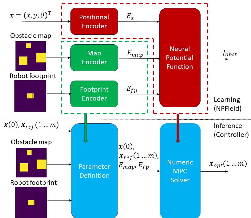
Figure 1: Common scheme of the proposed approach. Our controller (bottom half of the figure) consists of a parameter definition module and an MPC solver, which optimize the trajectory for a defined set of parameters. Our common neural architecture (NPField, top half of the figure) consists of image encoders and a neural potential function (NPFunction). We train NPFunction to predict the obstacle-repulsive potential for a given robot pose and given embeddings of the obstacle map and the robot footprint. The trained neural potential function is used for trajectory optimization within the MPC solver. Map and footprint encoders are removed from the optimization loop to decrease the dimensionality of the MPC problem. They are used for data preparation as both map and footprint are considered constant within the prediction horizon. More precise schemes of this architecture are given in figures 2 (Controller) and 3 (Network).

We propose a Neural Potential Field (NPField) – a neural network for calculating artificial potential. Our idea is conceptually inspired by the NeRF (Neural Radiance Field) model [12], which takes the position and orientation of the camera as an input and returns image intensity as an output. Our model takes the position and orientation of the robot together with the obstacle map and robot footprint as input and returns the value of repulsive potential as an output. We aim not to obtain this values themselves but to use the trained model within the optimization loop. There are several works where neural networks provide discrete costmaps in which values are used for search-based [13] or sampling-based planning [14, 15]. Our goal instead is to provide continuously differentiable function, which gradient is helpful for optimization. The key conceptual scheme of our approach is shown in Fig. 1.

MPC solvers are sensitive to the number of input parameters: a high number of parameters leads to a drastic increase in computational expenses. Map images should not be sent to the solver as they include many cells. We use image encoding within our architecture to reduce the number of parameters by replacing maps and footprints with their more compact embeddings. The top part of the fig. 1 presents our neural network architecture, while the bottom part shows the data flow of our controller. The neural network consists of two main parts: encoder block and Neural Potential Function (NPFunction) – a subnetwork that calculates the potential for a single robot configuration. Our controller consists of two high-level modules. The first module includes the algorithms, which define parameters for the MPC problem based on actual sensor data. Such a definition is made once per each iteration of the control loop. The second block includes a numerical solver for the control problem, which iteratively optimizes the trajectory based on the pre-defined parameters. NPField is trained as a single architecture and then divided into two parts. Image encoders are inserted into the parameter definition block, while NPFunction is integrated into the numerical MPC solver. For each controller step, encoders are called once, while NPFunction is called and differentiated multiple times within the optimization procedure.

I-A Contribution

This work mainly contributes in the following aspects:

• Novel architecture for MPC local planner, where the neural model estimates collision cost.

• Novel neural architecture for calculating APF based on the obstacle map, robot pose, and footprint.

• An approach for generating the dataset for training the neural model.

The last subsection of the next section provides a discussion on the place of our approach among the others.

I-B Structure

The rest of the paper is organized as follows. Section II discusses the related works. In section III, we introduce the architecture of our local planner. In section IV, we narrow down to our neural model and describe its architecture and learning. Section V discusses the experiments. Section VI is a conclusion section.

II RELATED WORKS

In this section we fist discuss common approaches to motion planning, then narrow down to collision avoidance in optimization based local planners. After that we discuss existing works, which use neural models within the MPC solvers. Finally we specify the differences of our approach compared to similar works.

II-A Planning

Planning task may be solved by various methods, which could be categorized into the following main groups (see review [16]): search-based planning (most of these methods are based on A* graph search algorithm [17], which is an extension of Dijkstra method [18]), sampling-based planning (most of these methods are based either on Rapidly-exploring Random Trees [19] or on Probabilistic RoadMaps [20]), motion primitives and trajectory optimization. We consider optimization-based planning in this work.

Depending on the statement, we can define two groups of planning tasks – global path planning (define a reference of intermediate robot configurations based on given initial and destination configuration) and local motion planning (define a smooth trajectory based on a given part of the global plan taking in mind kinodynamic constraints). The artificial potential field was initially proposed [10] for global planning: the robot’s path is obtained as a trajectory of the gradient descent in the potential field from the starting point towards the destination point. This planning approach can easily stuck in the local minimum. Therefore, it is less popular than A*, RRT, or PRM. However, it is still useful [21, 22, 23]. To avoid stucking in local minima, trajectory optimization is often done locally together with global planners [1, 7]. Global planner generates a rough suboptimal path, which is then optimized.

Trajectory optimization may be considered in two statements [1] - holistic computation (made offline before the motion; no strict real-time constraints) and model predictive control (sequential online optimization of near parts of the path during the motion). In the first case, there are no strict limits for the calculation time as well as for the length and complexity of the trajectory. There are some specfifc approaches for this case, such as CHOMP [24], STOMP [25], and TrajOpt [8]. CHOMP consider collision avoidance as constraints and therefore require collision-free initial guess. It may work with row representation of obstacles such as Occupancy Grid or Voxel Map for 3D planning tasks. TrajOpt consider collision avoidance as a penalty and may converge from initial guess, which include collision, however, it require obstacles to be represented as polytops. In the second case, the calculation time is limited according to the replanning rate of the system.

II-B Obstacle models for trajectory optimization

Collision detection itself is considered in many works, e.g., [26, 27, 28]; we are now interested in analytical models suitable for trajectory optimization. The safe path may be guaranteed using convex approximations of the free space [1, 11]. The disadvantage of such an approximation is that the free space outside the approximated region is prohibited. Alternatively, obstacles may be approximated instead of free space [4, 5, 7, 6]. Interception of the trajectory with the borderlines of the approximated regions may be modeled within the MPC solver. The approaches above require modeling either free space or obstacles as simple geometric shapes, such as points [4], circles [1, 5], polygons [6, 7], or polylines [29]. The question of how to obtain this representation from the common obstacle map is often not considered. Also, some approaches can be used only with discrete-time process models [7].

In the case when it is impossible or too complicated to provide differentiable collision models, one can use less stable techniques based on numerical gradients [8], stochastic gradients [25] or gradient-free sampling-based optimization (Model Predictive Path Integral [30, 31]). We consider another option, where a neural model approximates the repulsive potential. A number of works exist [32] on learning Control Barrier Functions for ensuring the safety of mobile systems such as drones [33] and cars [34] within the controller. The work [35] provides differentiable collision distance estimation for a 2D manipulator based on a graph neural network. [9] use the loss function of the network as a collision penalty: the trajectory is optimized during the network training for the fixed obstacle map.

II-C Neural Models within MPC Optimization

Integration of neural models into the MPC control loop was considered in a number of tasks. The challenging aspect here is the high computational cost of deep neural models. Accurate deep models by [36, 37] were not real-time and were presented in simulation as a proof of concept. Real-time inference may be achieved by significantly reducing model capacity [37]. Approaches [38, 39, 40] insert lightweight network into realtime MPC control loop. [41] achieve use of the deep neural model within real-time Acados MPC solver [42] by introducing ML-CasADI framework [43]. Experiments by [41] showed that direct insertion of the neural model into MPC-solver is effective for the networks with up to 50,000 parameters. Most works above use neural networks for approximating the model of process dynamics. On the contrary, we are interested in approximating obstacle-related cost terms and control barrier functions [33, 34, 32]. In [44], a neural network was used to update a cost function for manipulator visual servoing. Its architecture includes a neural encoder for camera images and a cost-update network for quadratic programming. There is also a set of works where a neural network was applied for choosing weighting factors for various terms of the cost function, e.g., [45, 46].

II-D Place of our approach among the others

We propose a neural model for estimating repulsive potential, which has the following properties. 1) It provides obstacle avoidance for mobile robotic platforms. 2) It is differentiable. 3) It exploits the capacity of deep neural models with more than 50,000 parameters. 4) It reproduces obstacle maps with complicated, non-convex structures and allows for optimization of long trajectories within this map. 5) It is integrated into the MPC controller for online solutions. 6) It includes map encoding, which provides dimensionality reduction and the ability to work with different maps. The following works seem to be the closest to ours concerning these properties. [9] satisfies 1), 2), and 4). However, it learns a trajectory for the single map offline. [44] satisfies 3), 5), and 6) however, it is intended for the different tasks. [33, 34] satisfy 1), 2), 3), and 5), however, they process vision data instead of obstacle map and work with simple-shaped obstacles. Other works satisfy less number of properties.

Unique property 7) of our approach is encoding the footprint of the mobile robot. It allows one to use a single model for mobile robots with different shapes. Note that in this work, we only prove a concept of footprint encoding: our training set consists of samples with two various footprints, and we show that the networks learn their collision model. We consider the deeper study of footprint learning (including footprint generalization) to be a part of the future work.

III Control approach

In this section, we discuss a model predictive controller, which is used for local planning. Neural networks are considered to be black boxes, which take inputs and provide outputs within the control architecture. Their internal content is discussed in a further section. We first describe the formal statement of a local optimization problem and then discuss the controller that solves this statement.

III-A MPC Statement

Local trajectory optimization may be formulated as a nonlinear model predictive control problem with continuous dynamics and discrete control:

$$\{\mathbf{x}_{opt}[i],\mathbf{u}_{opt}[i]\}_{i=k}^{k+p}=arg\min\sum_{i=k}^{k+p}J(\mathbf{x}[i],\mathbf{u}[i],\mathbf{p}[i]),$$ (1a)

s.t.

$$\frac{dx_{1}[i]}{dt}=f_{1}(\mathbf{x}[i],\mathbf{u}[i],\mathbf{p}[i]),$$ (1b)

$$\frac{dx_{2}[i]}{dt}=f_{2}(\mathbf{x}[i],\mathbf{u}[i],\mathbf{p}[i]),$$

$$\dots{\\ }\frac{dx_{\mu}[i]}{dt}=f_{\mu}(\mathbf{x}[i],\mathbf{u}[i],\mathbf{p}[i]),$$

$$h_{1}(\mathbf{x}[i],\mathbf{u}[i],\mathbf{p}[i])\leq 0,$$ (1c)

$$h_{2}(\mathbf{x}[i],\mathbf{u}[i],\mathbf{p}[i])\leq 0,$$

$$\dots{\\ }h_{\chi}(\mathbf{x}[i],\mathbf{u}[i],\mathbf{p}[i])\leq 0.$$

Here $p$ is prediction horizon, $\mathbf{x}[i]$ is $\mu$-size state vector (at the beginning of step $[i]$), $\mathbf{u}[i]$ is $\nu$-size control vector (constant within step $i$) $\mathbf{p}[i]$ is $\kappa$-vector of process parameters (relevant for the step $i$). (1a) specify the cost function $J$: a sum of functions $J[i]$, which are calculated for each node. (1b) define continuous dynamics of the process. (1c) is a set of inequality constraints which must be satisfied within the whole process. Optimization procedure aims to find the reference of $\{\mathbf{x}_{opt}[i],\mathbf{u}_{opt}[i]\}_{i=k}^{k+p}$ that provide minimum $J$. Note that in this work we use this statement for defining local trajectory of the robot (i.e. $\mathbf{x}_{opt}[i]_{i=k}^{k+m}$). Control of trajectory execution may be either provided by other control method or achieved by direct execution $u_{opt}$.

The view of the equation (1b) depend on the construction of the mobile robot. In this work we consider two different models: a differential drive model (relevant for our real-robot experiments) and a bicycle model (used in numerical experiments). Differential drive model is specified as follows:

$$\frac{dx}{dt}=v\cos\theta,$$ (2)

$$\frac{dy}{dt}=v\sin\theta,$$

$$\frac{dv}{dt}=a,$$

$$\frac{d\theta}{dt}=\omega.$$

State vector $\mathbf{x}=(x,y,v,\theta)^{T}$ include cartesian position of the robot $x,y$ , its linear velocity $v$, and its orientation $\theta$. Control vector $\mathbf{u}=(a,\omega)^{T}$ include linear acceleration $a$ and angular velocity $\omega$.

For bicycle model $\mathbf{u}=(a,\delta)^{T}$ where $\delta$ is steering angle. .

$$\frac{dx}{dt}=v\cos\theta,$$ (3)

$$\frac{dy}{dt}=v\sin\theta,$$

$$\frac{dv}{dt}=a,$$

$$\frac{d\theta}{dt}=\frac{v}{L}\tan\delta.$$

For the optimal control problem of this model, the following cost function is introduced:

$$J[i]=J_{s}(\mathbf{x}[i],\mathbf{u}[i],\mathbf{x}_{r}[i])+J_{o}(\mathbf{x}[i],\mathbf{p}_{o}[i]).$$ (4)

$J_{s}$ term enforce the trajectory to follow the reference values $\mathbf{x}_{r}$ from the global plan, while $J_{o}$ term push the trajectory farther from obstacles. $\mathbf{p}_{o}[i]$ is a vector of obstacle-related parameters. Whole parameter vector for the system (1) is $\mathbf{p}[i]=((\mathbf{x}_{r}[i])^{T},(\mathbf{p}_{o}[i])^{T})^{T}$. In our approach, the neural network is applied to compute $J_{o}$ while $J_{s}$ is calculated as follows:

$$J_{s}[i]=\sum_{j=1}^{\mu}w_{xj}(x_{j}[i]-x_{j(ref)}[i])^{2}+\sum_{k=1}^{\nu}w_{uk}u_{k}^{2}[i]\,$$ (5)

Here $w_{xj},w_{uk}$ are the weights of the respective terms, $x_{j(ref)}[i]$ is a reference value of the respective state (taken from the global plan).

Constraint-based trajectory optimizers like CIAO [1, 11] use equation (1c) to provide collision avoidance. Contrary, we express collision avoidance in (1a) and use (1c) only for box constraints of the separate variables.

III-B Control architecture

An architecture of our controller is shown in Fig. 2, which is a more detailed version of Fig. 1. Solution of the problem (1) is obtained iteratively using Sequential Quadratic Programming (optimization loop in Fig. 2). MPC controller uses the solution to update the trajectory online (control loop in Fig. 2). At the timestep $k$ it optimizes the trajectory for the next $p$ steps, and then the optimized control inputs are sent to the robot for the next $m$ steps (i.e. $m$ is the control horizon). After that optimization is repeated for the steps from $k+m$ to $k+m+p$.

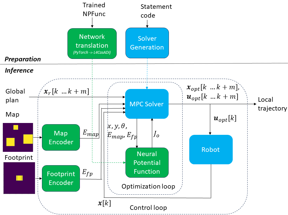
Figure 2: Proposed architecture of the controller. Image encoders work outside the optimization loop and we just need to run them once before each optimization procedure. NPFunction works within the optimization loop and the solver uses its gradients to find a safer trajectory.

MPC-solver is intended to provide solution of the problem (1) with (5) as (1a) and (2) as (1b). During optimization, it communicates with integrated NPFunction, which provides values and gradients of $J_{obst}$.

The objective of the neural network is to project the robot’s footprint, obstacle map, and robot poses onto a differentiable obstacle-repulsive potential surface. Consequently, for each coordinate within the range of the map, the neural network outputs a corresponding potential value. To ensure computational feasibility, we partitioned the neural network into two blocks: a map and footprint encoder, and a final coordinate potential predictor. Encoders compress high-dimensional maps into a compact representation, thereby enabling the computation of Jacobian and Hessian matrices of the control problem within the solver. Encoders work outside the optimization loop: provided embeddings $E_{map}$ and $E_{fp}$ are sent to the solver as obstacle-related problem parameters $\mathbf{p}_{o}$. This means that we assume the local map and robot footprint to be fixed within the prediction horizon. While the robot is following the global plan, the local map slides according to its current position and actual sensor data.

IV NEURAL POTENTIAL FIELD

In this section we discuss our neural model for calculating obstacle repulsive potential $J_{o}$. First, we briefly describe architecture of our network, then we introduce our strategy for generating the training set.

IV-A Network architecture

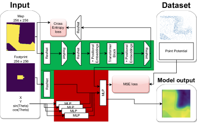
Figure 3: Proposed architecture of the neural network. The green component represents the robot footprint and map encoder, which generates embeddings that are consistent for all coordinates within the map. The red component signifies the final coordinate potential predictor, which contains an order of magnitude fewer parameters.

Proposed neural architecture is shown in Fig. 3. It consists of three primary components: a ResNet Encoder, a Spatial Transformer, and a ResNet Decoder. ResNet blocks are used with the objective of extracting local features from the obstacle map which contains a lot of corners and narrow passages. The Spatial Transformer utilizes the self-attention mechanism [47] to establish global relations among these features, assessing the significance of one feature in relation to others. Consequently, we employ the positional embedding technique from Visual Transformers [48]. Lastly, the ResNet Decoder processes the transformed feature maps to generate the final output.

To mitigate the model’s tendency to truncate critical details of the obstacle map necessary for navigation, we incorporated a map reconstruction loss based on Cross-Entropy. For the predictions of potential points, we employed the Mean Squared Error (MSE) loss.

IV-B Training data

One unit of the training set include $\{I_{map},I_{fp},x,y,\theta,J_{o}\}$, where $I_{map}$ and $I_{fp}$ are 2D images of the obstacle map and the robot footprint. The dataset should include various samples of robot positions from various maps. The maps are cropped from the MovingAI planning dataset [49]. For each map, we generate a set of random robot poses and calculate reference values for them using the following algorithm.

1. Obstacle map is transformed into a costmap:

   1. Signed distance function (SDF) is calculated algorithmically for each cell on the map. SDF is equal to the distance from the current cell to the nearest obstacle border. It is positive for free space cells and negative for obstacle cells.

   2. Repulsive potential is calculated for each cell: $J_{o}=w_{1}(\pi/2+arctan(w_{2}-w_{2}SDF))$. This is a sigmoid function, which is low far from obstacles, asymptotically strives to $w_{1}$ inside obstacles, and has maximum derivative on the obstacle border.

2. Collision potential is calculated for each random pose of the robot within the submap. For this purpose robot’s footprint is projected onto the map according to the pose. The maximum potential among the footprint-covered cells is chosen as a collision potential. As an alternative approach, we tried to compute collision potential as an integral potential over footprint. This trial did not provide learning of the useful potential function.

A pivotal aspect of the training process was the dataset sampling strategy. Utilizing a random sampling strategy across the map led to the network overfitting to larger values and disregarding narrow passages. This is because of the walls, which are statistically overwhelming compared to free space, but are irrelevant for navigation as we explicitly avoid planning through obstacles. To address this, we modified the sampling strategy such that 80% of points are sampled with intermediate potential values. The figure 4 shows the distribution of point samples in a map. The area with a high density of points represents the area surrounding and close to obstacles, while obstacles have a little effect on the path of movement in the areas with a low density of points.

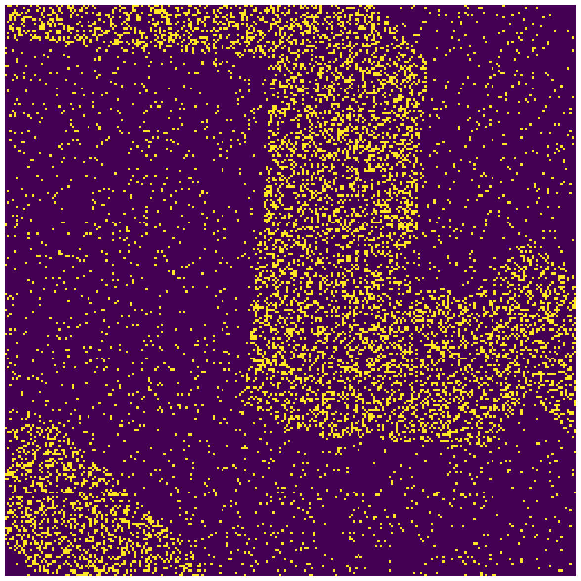
Figure 4: Example for distribution of samples in a map.

V Implementation

We consider nonlinear MPC task statement, which may be solved via Interior Point (IP) or Sequential Quadratic Programming (SQP). Modern frameworks provide the possibility for realtime execution of these methods. IPOPT [50] and ForcesPro [51] implement IP, while ACADO [52, 53] and Acados [42] implement SQP. These frameworks rely on a more low-level CasADi framework [54] for algorithmic differentiation. We implement our MPC solver with Acados framework, is which is the newest one and provide the fastest execution.

Use of deep neural network within Acados solver require the specific integration tool. Two libraries are relevant for this task: ML-CasADi [43] and L4CasADi [55]. Both provide the CasADi description of Pytorch [56] neural models. However, the first method was proposed and used for replacing complex models with local Taylor approximations to enable real-time optimization procedures, while the second method provides a complete mathematical description of the Pytorch model by CasADi formula. For our Pytorch model which describes the neural potential field of the obstacles surrounding the path of the robot, L4CasADi is more suitable because the description of the whole model is needed and not only at a linearizing point. ML provide lightweight local approximation of the complex neural model. This approximation constrain the use of ML-CasADi for the functions with complicated landscapes. Novel framework L4CasADi do not use such approximations. It provides integration of the deep neural models into real-time CasADi-based optimization. We use the L4CasADi to provide optimization over NPFunction. To our knowledge, our work is the first one, which exploits L4CasADi for neural cost terms instead of the neural dynamic model.

Our local planner works together with Theta* [57] global planner, which generates global plans as polylines. Note that Theta* uses a simplified version of the robot footprint (a circle with a diameter equal to the robot width) as it fails to provide a safe path with a complete footprint model. This simplified model does not guarantee the safety of the global plan, therefore the safety of the trajectory is provided by our local planner.

We consider obstacle maps to have a 256×256 resolution, where each pixel corresponds to 2×2 centimeters of the real environments (i.e. size of the map is 5.12×5.12 meters). We collected a dataset based on the MovingAI [49] city maps. It includes 4,000,000 samples taken from 200 maps with 2 footprints. Both footprints correspond to a real Husky UGV mobile manipulator with an UR5 robotic arm. The first one is with a folded arm, the second one is with an outstretched arm. 10,000 random poses of the robot were generated for each map with each footprint. Weighting coefficients for reference potential were set to $w_{1}=15$ and $w_{2}=10$, while the prediction horizon was set to $p=30$. Dataset generation took 40 hours on the Intel Core i5-10400F CPU.

Our neural network consists of 5 million parameters, with 500,000 allocated to ResNet encoders. Encoders project each (256×256) map and robot footprint into (1×4352) embeddings. The robot’s pose, represented as $X,Y,sin(\theta),cos(\theta)$, is transformed into (1,32) embeddings. The model was trained over a span of 24 hours on a server equipped with a single Nvidia Tesla V100 card with 32GB of memory.

VI Experiments

In this section we first present numerical comparison of our approach with other planning methods. Then we discuss effects of varying some hypreparameters of our method. Finally we show the experiments on a real robot.

VI-A Comparative studies

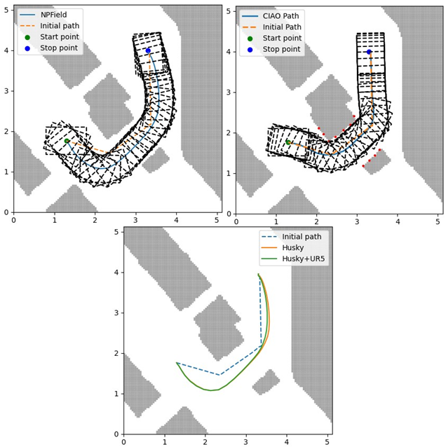
Figure 5: Example scenario for local planning. Left: NPField trajectory. Right: CIAO trajectory. Bottom: trajectory curves for different footprints.

All experiments reported in this subsection were 1) conducted with the bicycle model of process dynamics, and 2) conducted on the maps from the MovingAI dataset [49], which were not used for network training.

VI-A1 Illustrative example and comparison with trajectory optimizers

An example of the trajectory generated with our planner is shown in Fig. 6 on the left. A global plan in the form of a polyline is turned into a smooth and safe trajectory. Initially, the robot turns from the obstacle and deviates from the global path, then smoothly returns to it, reaching the goal position.

As a proof of concept for footprint encoding, we provide the following experiment. Consider the global plan, where the robot first moves towards the flat wall, then turns and moves parallel to the wall. In this case, a robot with a folded arm turns a little later than the one with a folded arm. Such a behavior may be seen in Fig. 6, bottom. The yellow curve relates to the outstretched arm, while the green curve relates to the folded arm. This behavior shows that the model learns different properties of two footprints, which are useful for safer trajectory planning.

We compared NPField trajectories with CIAO [1] trajectory optimizer, which is based on convex approximation of the free space around the robot. The CIAO-generated trajectory is shown in Fig. 6 on the right. It may be seen that it keeps the robot near obstacles, nearly touching their edges. When testing on more diverse scenarios, CIAO could not find the feasible path in nearly half of the cases. It may be connected with the fact that CIAO implements collision avoidance as a set of inequality constraints, which are not differentiated during optimization. Therefore, it only checks the fact of the collision and does not balance between safety and path deviation in the cost function.

VI-A2 Comparison on BenchMR

We compare our algorithm with the baselines on 20 scenarios using BenchMR [58] framework. The tasks include moving through the narrow passages similar to those shown in Fig. 6. We compare standard metrics: planning time, path length, smoothness, and angle-over-length (for all, lower value is better). We also introduce our custom metric, ”safety distance” (minimum value of the SDF).

Planner	Time, s	Length, m	Smooth-ness	AOL	Safety distance, m
RRT*	11	2.27	0.008	0.005	0.048
RRT	0.013	2.72	0.012	0.010	0.148
InformedRRT	11	2.27	0.006	0.004	0.041
SBL	0.062	4.99	0.055	0.042	0.049
RRT+GRIPS	0.013	2.44	0.009	0.004	0.151
$\theta*$+NPField (ours)	0.063	2.33	0.002	0.006	0.116

TABLE I: Comparative studies on BenchMR scenarios

The results are given in table I. We compare our stack (Theta* + NPField) with state of the art planners: RRT [19], RRT* [59], Informed RRT [60], SBL [61] and RRT with GRIPS [62] smoothing. We do not provide the results for PRM [20], PRM* [59], BIT* [63], KPIECE1 [64], Theta* with CIAO [1] optimization, Theta* with CHOMP [8] optimization as they were able to generate a successful plan for less than a half of tasks. This result is particularly important for Theta* + CIAO and Theta* + CHOMP, as they are optimization-based planers similar to our approach and use the same global plans. However, they could not handle considered scenarios due to collisions (CHOMP) or failure to find a result (CIAO). Results in the table show that our stack is generally comparable to other planners. It provides nearly the shortest path length, the best smoothness, a good AOL, and a good safety distance.

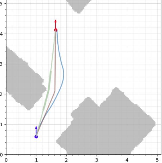
Figure 6: Example comparison of NPField (blue curve) and CHOMP (green curve). CHOMP converges to the shortest path ignoring obstacle danger.

Computation time has the same order of magnitude with the fastest methods. We cannot specify an approach, which is definitely better than ours (RRT with GRIPS is fast and safe but provides less smooth trajectories). Performance measurements were made on Intel Core i5-10400F CPU. Note that Acados solver need to warmup before reatime use: first execution of the optimization procedure may take about one second; after that the solver work faster. One optimization take 60-70 ms, where data encoding take around 10 ms, while Acados solution take the rest 50-60 ms.

VI-B Ablation studies

We also compare various versions of our algorithm on the same set of scenarios. These versions are different each other by the weights of the potential function which is used to calculate the potentials in training dataset, the features used for training the model, or the distribution the sampling points in the training maps.

First, we consider the situation when the reference collision potential (see subsection IV.B) is calculated as an integral value over footprint instead of choosing the maximum value. We had a hypothesis that such an approach could lead to better learning of the relative geometry of the object. However, it did not lead to an useful model. In our experiments the network provides incorrect results systematically (example is given in Fig. 7).

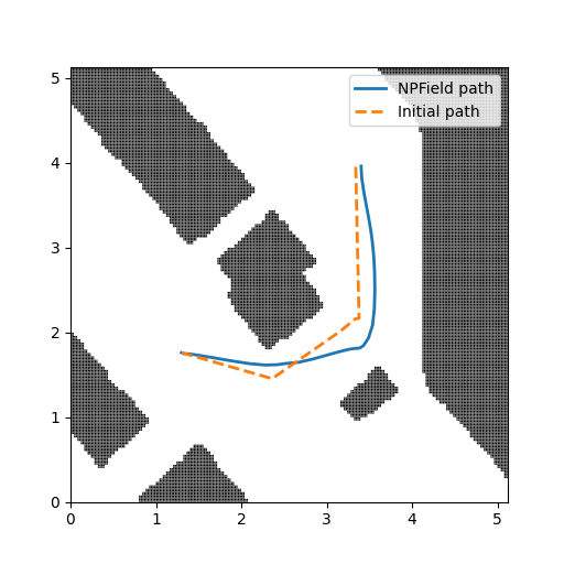
Figure 7: Example of path with integral potential

Similar incorrect results were measured for an alternative choice of weighting coefficient $w_{2}$ for calculating the training values of the repulsive potential. The idea was to make the potential landscape more gentle and provide better optimization from incorrect initial guess. In practice it lead to bad learning of the map properties, see example rezult for $w_{2}=1$ in Fig. 8.

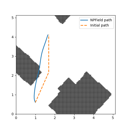
Figure 8: Example of path with different weights model

Our third ablation experiment was connected with the varying resolution of the obstacle map and robot footprint. We consider the situation when one cell of the grid correspond to 10x10 cm instead of 2x2 cm. These two sets are specified by a practical resolution of the global map and the local map respectively. The global map of the environment is stored in the memory of the robot, while the local map include actual data from the sensors. The size of the submap is 50x50 pixels (i.e. 5x5 meters). This size allow us to reduce the complexity of the neural network: total number of parameters is 1.4M instead of 5M; the size of the map embedding is 1161 instead of 4352. This archintucture still allow correct solution of the planning task; examples are provided in Fig. 9. Surprisingly reducing the model complexity did not affect the performance of the solver: it still take around 70 ms to make an optimization.

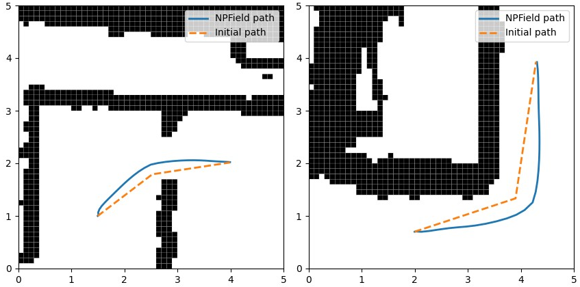
Figure 9: Example of paths on a low-resolution map.

VI-C Real Robot Experiments

We deploy our approach on a real Husky UGV mobile manipulator as a ROS module for MPC local planning and control, which works with Theta* global planner. The testing scenario includes hat transportation through a twisty corridor. The manipulator is holding the hat in an outstretched configuration (see Fig. 10). Acados optimizer run Intel Core i5-10400F CPU and communicate with the robot in real time as a remote ROS-node with control horizon equal to one step. Therefore, a more complicated concave footprint is valid. Scenario execution may be seen in the accompanying video (see https://github.com/cog-isa/NPField).

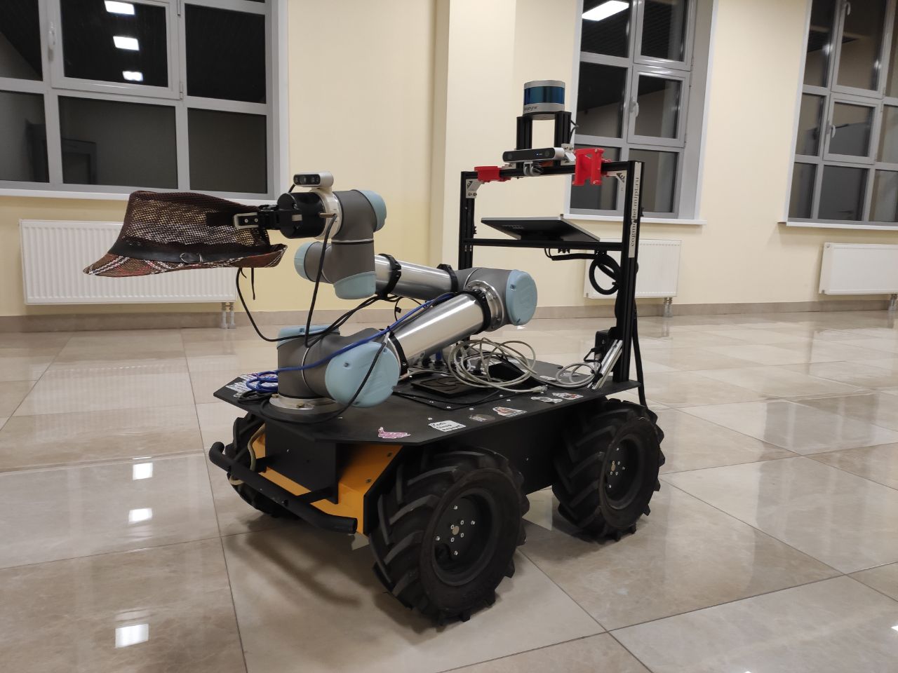
Figure 10: Husky mobile manipulator transforming a hat. A footprint with an outstretched manipulator is valid for this task.

VII CONCLUSIONS

We propose a novel approach to local trajectory planning, where a Model Predictive Controller uses the neural model to estimate collision danger as a differentiable function. Our NPField neural architecture consists of encoders and NPFunction blocks. Encoders provide a compact representation of the obstacle map and robot footprint; this compact representation is sent to the MPC solver as a vector of problem parameters. NPFunction is integrated into the optimization loop, and its gradients are used for trajectory correction. We implement our controller using Acados MPC framework and L4CasADi tool for integrating deep neural models into MPC loop. Our approach allows the robot with a complicated footprint to successfully navigate among the obstacles in real time. A planning stack Theta* + NPField showed comparable results with sample-based planners on the BenchMR testing framework. The code for our approach is presented at https://github.com/cog-isa/NPField.

We consider our work a starting point for further research on neural potential estimation for kinodynamic planning for various robotic systems in various environments. Trajectory planning on more complex maps (e.g. elevation maps) is a promising topic of the future research. Another important aspect is further research on footprint encoding, which may be useful for planning the trajectories of the robotic system with changing footprints (e.g. mobile manipulators under whole-body control).

References

- [1] Tobias Schoels, Luigi Palmieri, Kai O. Arras and Moritz Diehl “An NMPC Approach using Convex Inner Approximations for Online Motion Planning with Guaranteed Collision Avoidance” In 2020 IEEE International Conference on Robotics and Automation (ICRA), 2020, pp. 3574–3580 DOI: 10.1109/ICRA40945.2020.9197206
- [2] Damir Bojadžić et al. “Non-holonomic RRT & MPC: Path and trajectory planning for an autonomous cycle rickshaw” In arXiv preprint arXiv:2103.06141, 2021
- [3] Zhiqiang Zuo et al. “MPC-based cooperative control strategy of path planning and trajectory tracking for intelligent vehicles” In IEEE Transactions on Intelligent Vehicles 6.3 IEEE, 2020, pp. 513–522
- [4] Jie Ji, Amir Khajepour, Wael William Melek and Yanjun Huang “Path planning and tracking for vehicle collision avoidance based on model predictive control with multiconstraints” In IEEE Transactions on Vehicular Technology 66.2 IEEE, 2016, pp. 952–964
- [5] Jun Zeng, Bike Zhang and Koushil Sreenath “Safety-critical model predictive control with discrete-time control barrier function” In 2021 American Control Conference (ACC), 2021, pp. 3882–3889 IEEE
- [6] Lars Blackmore, Masahiro Ono and Brian C Williams “Chance-constrained optimal path planning with obstacles” In IEEE Transactions on Robotics 27.6 IEEE, 2011, pp. 1080–1094
- [7] Akshay Thirugnanam, Jun Zeng and Koushil Sreenath “Safety-Critical Control and Planning for Obstacle Avoidance between Polytopes with Control Barrier Functions” In 2022 International Conference on Robotics and Automation (ICRA), 2022, pp. 286–292 DOI: 10.1109/ICRA46639.2022.9812334
- [8] John Schulman et al. “Motion planning with sequential convex optimization and convex collision checking” In The International Journal of Robotics Research 33, 2014, pp. 1251–1270
- [9] Mikhail Kurenkov et al. “NFOMP: Neural Field for Optimal Motion Planner of Differential Drive Robots With Nonholonomic Constraints” In IEEE Robotics and Automation Letters 7.4, 2022, pp. 10991–10998 DOI: 10.1109/LRA.2022.3196886
- [10] O. Khatib “Real-time obstacle avoidance for manipulators and mobile robots” In Proceedings. 1985 IEEE International Conference on Robotics and Automation 2, 1985, pp. 500–505 DOI: 10.1109/ROBOT.1985.1087247
- [11] Tobias Schoels et al. “CIAO*: MPC-based Safe Motion Planning in Predictable Dynamic Environments” 21st IFAC World Congress In IFAC-PapersOnLine 53.2, 2020, pp. 6555–6562 DOI: https://doi.org/10.1016/j.ifacol.2020.12.072
- [12] Ben Mildenhall et al. “NeRF: Representing Scenes as Neural Radiance Fields for View Synthesis”, 2020 arXiv:2003.08934 [cs.CV]
- [13] Daniil Kirilenko, Anton Andreychuk, Aleksandr Panov and Konstantin Yakovlev “TransPath: Learning Heuristics for Grid-Based Pathfinding via Transformers” In Proceedings of the AAAI Conference on Artificial Intelligence 37.10, 2023, pp. 12436–12443 DOI: 10.1609/aaai.v37i10.26465
- [14] Samuel Triest et al. “Learning Risk-Aware Costmaps via Inverse Reinforcement Learning for Off-Road Navigation” In arXiv preprint arXiv:2302.00134, 2023
- [15] Mateo Guaman Castro et al. “How does it feel? self-supervised costmap learning for off-road vehicle traversability” In 2023 IEEE International Conference on Robotics and Automation (ICRA), 2023, pp. 931–938 IEEE
- [16] David González, Joshué Pérez, Vicente Milanés and Fawzi Nashashibi “A Review of Motion Planning Techniques for Automated Vehicles” In IEEE Transactions on Intelligent Transportation Systems 17.4, 2016, pp. 1135–1145 DOI: 10.1109/TITS.2015.2498841
- [17] Peter E. Hart, Nils J. Nilsson and Bertram Raphael “A Formal Basis for the Heuristic Determination of Minimum Cost Paths” In IEEE Transactions on Systems Science and Cybernetics 4.2, 1968, pp. 100–107 DOI: 10.1109/TSSC.1968.300136
- [18] Edsger W Dijkstra “A note on two problems in connexion with graphs” In Numerische mathematik 1.1, 1959, pp. 269–271
- [19] Steven M. LaValle and Jr. James J. “Randomized Kinodynamic Planning” In The International Journal of Robotics Research 20.5, 2001, pp. 378–400 DOI: 10.1177/02783640122067453
- [20] L.E. Kavraki, P. Svestka, J.-C. Latombe and M.H. Overmars “Probabilistic roadmaps for path planning in high-dimensional configuration spaces” In IEEE Transactions on Robotics and Automation 12.4, 1996, pp. 566–580 DOI: 10.1109/70.508439
- [21] Dong Hun Kim and Seiichi Shin “Local path planning using a new artificial potential function composition and its analytical design guidelines” In Advanced Robotics 20, 2006, pp. 115–135
- [22] Jing Ren, K.A. McIsaac and R.V. Patel “Modified Newton’s method applied to potential field-based navigation for mobile robots” In IEEE Transactions on Robotics 22.2, 2006, pp. 384–391 DOI: 10.1109/TRO.2006.870668
- [23] Rafal Szczepanski, Tomasz Tarczewski and Krystian Erwinski “Energy Efficient Local Path Planning Algorithm Based on Predictive Artificial Potential Field” In IEEE Access 10, 2022, pp. 39729–39742 DOI: 10.1109/ACCESS.2022.3166632
- [24] Nathan Ratliff, Matt Zucker, J. Bagnell and Siddhartha Srinivasa “CHOMP: Gradient optimization techniques for efficient motion planning” In 2009 IEEE International Conference on Robotics and Automation, 2009, pp. 489–494 DOI: 10.1109/ROBOT.2009.5152817
- [25] Mrinal Kalakrishnan et al. “STOMP: Stochastic trajectory optimization for motion planning” In Proceedings - IEEE International Conference on Robotics and Automation, 2011, pp. 4569–4574 DOI: 10.1109/ICRA.2011.5980280
- [26] Elmer G Gilbert, Daniel W Johnson and S Sathiya Keerthi “A fast procedure for computing the distance between complex objects in three-dimensional space” In IEEE Journal on Robotics and Automation 4.2 IEEE, 1988, pp. 193–203
- [27] Simon Zimmermann et al. “Differentiable collision avoidance using collision primitives” In 2022 IEEE/RSJ International Conference on Intelligent Robots and Systems (IROS), 2022, pp. 8086–8093 IEEE
- [28] Zeqing Zhang et al. “A generalized continuous collision detection framework of polynomial trajectory for mobile robots in cluttered environments” In IEEE Robotics and Automation Letters 7.4 IEEE, 2022, pp. 9810–9817
- [29] Julius Ziegler, Philipp Bender, Thao Dang and Christoph Stiller “Trajectory planning for Bertha — A local, continuous method” In 2014 IEEE Intelligent Vehicles Symposium Proceedings, 2014, pp. 450–457 DOI: 10.1109/IVS.2014.6856581
- [30] Grady Williams et al. “Aggressive driving with model predictive path integral control” In 2016 IEEE International Conference on Robotics and Automation (ICRA), 2016, pp. 1433–1440
- [31] Grady Williams et al. “Information theoretic MPC for model-based reinforcement learning” In 2017 IEEE International Conference on Robotics and Automation (ICRA), 2017, pp. 1714–1721 IEEE
- [32] Charles Dawson, Sicun Gao and Chuchu Fan “Safe control with learned certificates: A survey of neural lyapunov, barrier, and contraction methods for robotics and control” In IEEE Transactions on Robotics IEEE, 2023
- [33] Michal Adamkiewicz et al. “Vision-Only Robot Navigation in a Neural Radiance World” In IEEE Robotics and Automation Letters 7.2, 2022, pp. 4606–4613 DOI: 10.1109/LRA.2022.3150497
- [34] Hossein Abdi, Golnaz Raja and Reza Ghabcheloo “Safe Control using Vision-based Control Barrier Function (V-CBF)” In 2023 IEEE International Conference on Robotics and Automation (ICRA), 2023, pp. 782–788 IEEE
- [35] Yeseung Kim, Jinwoo Kim and Daehyung Park “GraphDistNet: A Graph-Based Collision-Distance Estimator for Gradient-Based Trajectory Optimization” In IEEE Robotics and Automation Letters 7.4 IEEE, 2022, pp. 11118–11125
- [36] Ali Punjani and Pieter Abbeel “Deep learning helicopter dynamics models” In 2015 IEEE International Conference on Robotics and Automation (ICRA), 2015, pp. 3223–3230 DOI: 10.1109/ICRA.2015.7139643
- [37] Alessandro Saviolo, Guanrui Li and Giuseppe Loianno “Physics-Inspired Temporal Learning of Quadrotor Dynamics for Accurate Model Predictive Trajectory Tracking” In IEEE Robotics and Automation Letters 7.4, 2022, pp. 10256–10263 DOI: 10.1109/LRA.2022.3192609
- [38] Nathan A. Spielberg, Matthew Brown and J. Gerdes “Neural Network Model Predictive Motion Control Applied to Automated Driving With Unknown Friction” In IEEE Transactions on Control Systems Technology 30.5, 2022, pp. 1934–1945 DOI: 10.1109/TCST.2021.3130225
- [39] Kong Yao Chee, Tom Z. Jiahao and M. Hsieh “KNODE-MPC: A Knowledge-Based Data-Driven Predictive Control Framework for Aerial Robots” In IEEE Robotics and Automation Letters 7.2, 2022, pp. 2819–2826 DOI: 10.1109/LRA.2022.3144787
- [40] Taekyung Kim, Hojin Lee, Seongil Hong and Wonsuk Lee “TOAST: Trajectory Optimization and Simultaneous Tracking Using Shared Neural Network Dynamics” In IEEE Robotics and Automation Letters 7.4 IEEE, 2022, pp. 9747–9754
- [41] Tim Salzmann et al. “Real-Time Neural MPC: Deep Learning Model Predictive Control for Quadrotors and Agile Robotic Platforms” In IEEE Robotics and Automation Letters 8.4, 2023, pp. 2397–2404 DOI: 10.1109/LRA.2023.3246839
- [42] Robin Verschueren et al. “Acados: a modular open-source framework for fast embedded optimal control”, 2020 arXiv:1910.13753 [math.OC]
- [43] Tim Salzmann “TUM-AAS/ml-casadi: Use PyTorch Models with CasADi and Acados”, 2023 URL: https://github.com/TUM-AAS/ml-casadi
- [44] Avadesh Meduri, Huaijiang Zhu, Armand Jordana and Ludovic Righetti “MPC with Sensor-Based Online Cost Adaptation” In 2023 IEEE International Conference on Robotics and Automation (ICRA), 2023, pp. 996–1002 IEEE
- [45] Mateja Novak, Tomislav Dragicevic and Frede Blaabjerg “Weighting factor design based on Artificial Neural Network for Finite Set MPC operated 3L-NPC converter” In 2019 IEEE Applied Power Electronics Conference and Exposition (APEC), 2019, pp. 77–82 IEEE
- [46] Xin Wang, Yuan Gao, Jason Atkin and Serhiy Bozhko “Neural network based weighting factor selection of mpc for optimal battery and load management in mea” In 2020 23rd International Conference on Electrical Machines and Systems (ICEMS), 2020, pp. 1763–1768 IEEE
- [47] Ashish Vaswani et al. “Attention Is All You Need”, 2023 arXiv:1706.03762 [cs.CL]
- [48] Alexey Dosovitskiy et al. “An Image is Worth 16x16 Words: Transformers for Image Recognition at Scale”, 2021 arXiv:2010.11929 [cs.CV]
- [49] N. Sturtevant “Benchmarks for Grid-Based Pathfinding” In Transactions on Computational Intelligence and AI in Games 4.2, 2012, pp. 144–148 URL: http://web.cs.du.edu/~sturtevant/papers/benchmarks.pdf
- [50] Waechter Andreas and Biegler Lorenz T. “IPOPT, url=https:// github.com/coin-or/Ipopt”, 2005–2022
- [51] A. Zanelli, A. Domahidi, J. Jerez and M. Morari “FORCES NLP: an efficient implementation of interior-point methods for multistage nonlinear nonconvex programs” In International Journal of Control, 2017, pp. 1–17
- [52] B. Houska, H.J. Ferreau and M. Diehl “ACADO Toolkit – An Open Source Framework for Automatic Control and Dynamic Optimization” In Optimal Control Applications and Methods 32.3, 2011, pp. 298–312
- [53] B. Houska, H.J. Ferreau and M. Diehl “An Auto-Generated Real-Time Iteration Algorithm for Nonlinear MPC in the Microsecond Range” In Automatica 47.10, 2011, pp. 2279–2285 DOI: 10.1016/j.automatica.2011.08.020
- [54] Joel A E Andersson et al. “CasADi – A software framework for nonlinear optimization and optimal control” In Mathematical Programming Computation 11.1 Springer, 2019, pp. 1–36 DOI: 10.1007/s12532-018-0139-4
- [55] Tim Salzmann “GitHub - Tim-Salzmann/l4casadi: Use PyTorch Models with CasADi and Acados”, 2023 URL: https://github.com/Tim-Salzmann/l4casadi
- [56] Adam Paszke et al. “Pytorch: An imperative style, high-performance deep learning library” In Advances in neural information processing systems 32, 2019
- [57] Alex Nash, Kenny Daniel, Sven Koenig and Ariel Felner “Theta^*: Any-angle path planning on grids” In AAAI 7, 2007, pp. 1177–1183
- [58] Eric Heiden et al. “Bench-MR: A Motion Planning Benchmark for Wheeled Mobile Robots” In IEEE Robotics and Automation Letters 6.3, 2021, pp. 4536–4543 DOI: 10.1109/LRA.2021.3068913
- [59] Sertac Karaman and Emilio Frazzoli “Sampling-based algorithms for optimal motion planning” In The international journal of robotics research 30.7 Sage Publications Sage UK: London, England, 2011, pp. 846–894
- [60] Jonathan D Gammell, Siddhartha S Srinivasa and Timothy D Barfoot “Informed RRT: Optimal sampling-based path planning focused via direct sampling of an admissible ellipsoidal heuristic” In 2014 IEEE/RSJ international conference on intelligent robots and systems, 2014, pp. 2997–3004 IEEE
- [61] David Hsu, J-C Latombe and Rajeev Motwani “Path planning in expansive configuration spaces” In Proceedings of international conference on robotics and automation 3, 1997, pp. 2719–2726 IEEE
- [62] Eric Heiden et al. “Gradient-informed path smoothing for wheeled mobile robots” In 2018 IEEE International Conference on Robotics and Automation (ICRA), 2018, pp. 1710–1717 IEEE
- [63] Jonathan D Gammell, Timothy D Barfoot and Siddhartha S Srinivasa “Batch Informed Trees (BIT*): Informed asymptotically optimal anytime search” In The International Journal of Robotics Research 39.5 SAGE Publications Sage UK: London, England, 2020, pp. 543–567
- [64] Ioan A Sucan and Lydia E Kavraki “Kinodynamic motion planning by interior-exterior cell exploration” In Algorithmic Foundation of Robotics VIII 57 Springer Berlin; Heidelberg, Germany, 2009, pp. 449–464