The $\nu_{R}$-philic scalar dark matter

Abstract

Right-handed neutrinos ($\nu_{R}$) offer an intriguing portal to new physics in hidden sectors where dark matter (DM) may reside. In this work, we delve into the simplest hidden sector involving only a real scalar exclusively coupled to $\nu_{R}$, referred to as the $\nu_{R}$-philic scalar. We investigate the viability of the $\nu_{R}$-philic scalar to serve as a DM candidate, under the constraint that the coupling of $\nu_{R}$ to the standard model is determined by the seesaw relation and is responsible for the observed DM abundance. By analyzing the DM decay channels and solving Boltzmann equations, we identify the viable parameter space. In particular, our study reveals a lower bound ($\sim 10^{4}$ GeV) on the mass of $\nu_{R}$ for the $\nu_{R}$-philic scalar to be DM. The DM mass may vary from sub-keV to sub-GeV. Within the viable parameter space, monochromatic neutrino lines from DM decay can be an important signal for DM indirect detection.

1 Introduction

Right-handed neutrinos ($\nu_{R}$) are among the most compelling extensions of the Standard Model (SM), offering a simple solution to the problems of neutrino mass and matter-antimatter asymmetry. Given that the observed dark matter (DM) in our universe is also evidence of new physics beyond the SM, it is tempting to consider potential connections between $\nu_{R}$ and DM.

Being nearly invisible, right-handed neutrinos themselves have long been considered as a popular DM candidate, known as keV sterile neutrino DM—see Refs. Dasgupta:2021ies ; Abazajian:2017tcc ; Drewes:2016upu for recent reviews. However, the simplest scenario achieved via the Dodelson–Widrow mechanism Dodelson:1993je has been ruled out by X-ray and Lyman-$\alpha$ observations Dasgupta:2021ies ; Palanque-Delabrouille:2019iyz .

Due to their singlet nature, right-handed neutrinos are also considered as a portal to more hidden sectors, where a DM candidate may reside. For instance, one can introduce a dark fermion-scalar pair, $\chi\text{-}\phi$, with the interaction ${\cal L}\supset\nu_{R}\chi\phi$. This is the minimal framework to accommodate absolutely stable DM in the $\nu_{R}$ sector and has been investigated extensively in the literature Pospelov:2007mp ; Falkowski:2009yz ; Gonzalez-Macias:2016vxy ; Escudero:2016ksa ; Tang:2016sib ; Batell:2017rol ; Bandyopadhyay:2018qcv ; Becker:2018rve ; Chianese:2018dsz ; Folgado:2018qlv ; Chianese:2019epo ; Hall:2019rld ; Blennow:2019fhy ; Bandyopadhyay:2020qpn ; Hall:2021zsk ; Chianese:2021toe ; Biswas:2021kio ; Coy:2021sse ; Coy:2022xfj ; Barman:2022scg ; Coito:2022kif ; Li:2022bpp . Within this framework, the relic abundance of DM depends not only on the coupling of $\nu_{R}\chi\phi$, but also on the coupling of $\nu_{R}$ with the SM. If the $\nu_{R}$-SM coupling is sufficiently weak while $\nu_{R}$ dominantly decays to $\chi$ and $\phi$, the DM abundance depends only on the $\nu_{R}$-SM coupling Coy:2021sse ; Coy:2022xfj . Assuming the $\nu_{R}$-SM coupling is related to neutrino masses via the type-I seesaw relation, the DM abundance largely depends on the $\nu_{R}$-DM coupling since the type-I seesaw Yukawa coupling can maintain thermal equilibrium between $\nu_{R}$ and the SM Barman:2022scg . A comprehensive study that systematically investigates all possible scenarios can be found in Ref. Li:2022bpp .

In this work, we consider a further simplified framework in which the dark sector contains only a scalar singlet $\phi$ and it is exclusively coupled to $\nu_{R}$ Dudas:2014bca . We refer to it as the $\nu_{R}$-philic scalar. Despite its simplicity, the $\nu_{R}$-philic scalar as a DM candidate has drawn less attention since it lacks absolute stability. Nevertheless, the absolute stability is not fundamentally necessary for a DM candidate. It is possible, with a small coupling, that the $\nu_{R}$-philic scalar can have a sufficiently long lifetime. Therefore, we are curious about whether the $\nu_{R}$-philic scalar, as the minimal dark sector built on $\nu_{R}$, can be a DM candidate or not.

In this paper, we present a dedicated analysis of possible decay channels of the $\nu_{R}$-philic scalar $\phi$, solve the Boltzmann equation of $\phi$, and identify the viable parameter space for it to be DM. We find that, to serve as a DM candidate, the $\nu_{R}$-philic scalar needs to be lighter than $\sim 200$ MeV while the $\nu_{R}$ mass needs to be above $\sim 10^{4}$ GeV, provided that the $\nu_{R}$-SM coupling is determined by the seesaw relation.

The $\nu_{R}$-philic scalar DM shares some similarities with the Majoron DM Berezinsky:1993fm ; Bazzocchi:2008fh ; Gu:2010ys ; Frigerio:2011in ; Lattanzi:2013uza ; Queiroz:2014yna ; Boucenna:2014uma ; Garcia-Cely:2017oco ; Reig:2019sok ; Akita:2023qiz . The Majoron, with the name implying its relevance to the generation of the Majorana mass of $\nu_{R}$, is primarily coupled to $\nu_{R}$ and could be included in our $\nu_{R}$-philic scalar framework. However, as a Goldstone boson arising from the lepton number symmetry breaking, the Majoron would be massless in the minimal construction Chikashige:1980ui . To be DM, it has to possess a mass, which is typically introduced via soft-breaking terms. For example, in Ref. Frigerio:2011in , a Majoron-Higgs quartic term was introduced to simultaneously account for both the Majoron mass and the relic abundance. In the presence of such additional interactions, our conclusion in general does not apply but our analysis can be considered as a case study in the vanishing limit of additional interactions.

Our work is structured as follows. In Sec. 2, we introduce the model considered in this work as well as some basic formulae for our analysis. In Sec. 3, we discuss the dominant decay channels of the $\nu_{R}$-philic scalar, compute the decay widths, and estimate the thermal production of DM in the early universe. This allows us to identify the viable parameter space in an almost analytical approach, while the results are further supported by numerically solving the Boltzmann equations in Sec. 4. In Sec. 5, we discuss possible neutrino signals from DM decay as an observational consequence of this model. Finally we conclude in Sec. 6 and relegate some detailed calculations to the appendix.

2 Basic setup

2.1 The Lagrangian

We consider the standard Type-I seesaw model extended by a scalar singlet. The full Lagrangian of the model considered in this work reads:

$${\cal L}={\cal L}_{{\rm SM}}+{\cal L}_{{\rm seesaw}}+\frac{1}{2}(\partial\phi)^{2}-\frac{1}{2}m_{\phi}^{2}\phi^{2}+\left(\frac{y}{2}\thinspace\nu_{R}\nu_{R}\phi+{\rm h.c.}\right),$$ (2.1)

where $\phi$ is a real scalar with mass $m_{\phi}$ and couples only to $\nu_{R}.$ The SM Lagrangian is denoted by ${\cal L}_{{\rm SM}}$ and the seesaw Lagrangian is given by

$${\cal L}_{{\rm seesaw}}=\nu_{R}^{\dagger}\overline{\sigma}^{\mu}i\partial_{\mu}\nu_{R}-\left(\frac{m_{R}}{2}\nu_{R}\nu_{R}+{\rm h.c.}\right)+\left(y_{\nu}\tilde{H}^{\dagger}L\nu_{R}+{\rm h.c.}\right),$$ (2.2)

where $\tilde{H}\equiv i\sigma_{2}H^{*}$ with $H$ the SM Higgs doublet, and $L=\left(\nu_{L},\ e_{L}\right)^{T}$ is the lepton doublet. In this work, for simplicity, we do not consider the flavor structure within the neutrino sector. Consequently, we treat $y$, $m_{R}$, and $y_{\nu}$ as single values rather than matrices. Additionally, we adopt the notation of two-component Weyl spinors, following the convention established in Ref. Dreiner:2008tw .

At low-energy scales after electroweak symmetry breaking, ${\cal L}_{{\rm seesaw}}$ generates neutrino masses via the well-known seesaw relation

$$m_{\nu}=\frac{m_{D}^{2}}{m_{R}}\thinspace,\ m_{D}=\frac{y_{\nu}v}{\sqrt{2}}\thinspace,$$ (2.3)

where $v\approx 246$ GeV is the electroweak vacuum expectation value (VEV), $m_{D}$ is the Dirac mass of neutrinos generated by the Higgs mechanism, and $m_{\nu}={\cal O}(0.1)$ eV is the neutrino mass responsible for neutrino oscillations.

Throughout this work, we assume that the $\nu_{R}$-SM coupling $y_{\nu}$ is determined by Eq. (2.3), i.e., $y_{\nu}=\sqrt{2m_{\nu}m_{R}}/v$.

2.2 The Boltzmann equation

In the expanding universe, the number density of $\phi$, denoted by $n_{\phi},$ is governed by the Boltzmann equation:

$$\frac{dn_{\phi}}{dt}+3Hn_{\phi}=C_{\text{prod}}-C_{\text{depl}}\thinspace,$$ (2.4)

where $H$ is the Hubble parameter, and $C_{\text{prod}}$ and $C_{\text{depl}}$ denote the collision terms responsible for the production and depletion of $\phi$, respectively. Since the left-hand side can also be written as $a^{-3}d(n_{\phi}a^{3})/dt$, $C_{\text{prod}}$ and $C_{\text{depl}}$ can be physically interpreted as the number of $\phi$ being produced and depleted per unit time per comoving volume.

For convenience, we introduce $g_{H}\equiv\sqrt{8\pi^{3}g_{\star}/90}$ with $g_{\star}$ the effective number of relativistic degrees of freedom in the thermal bath, such that

$$H=g_{H}\frac{T^{2}}{m_{{\rm pl}}}\thinspace,$$ (2.5)

where $T$ is the temperature of the SM thermal bath and $m_{{\rm pl}}=1.22\times 10^{19}$ GeV is the Planck mass.

If $\phi$ reaches thermal equilibrium, its number density is given by

$$n_{\phi}^{{\rm eq}}=\int\frac{1}{e^{E/T}-1}\frac{d^{3}p}{(2\pi)^{3}}=\begin{cases}\zeta(3)\frac{T^{3}}{\pi^{2}}&(T\gg m_{\phi})\\[5.69054pt] \left(\frac{m_{\phi}T}{2\pi}\right)^{3/2}e^{-m_{\phi}/T}&(T\ll m_{\phi})\end{cases}\thinspace,$$ (2.6)

where $\zeta$ is the Riemann zeta function and $\zeta(3)\approx 1.202$.

The DM relic abundance $\Omega_{\phi}h^{2}$ is related to $n_{\phi}$ via

$$\Omega_{\phi}h^{2}=0.12\times\left.\frac{m_{\phi}n_{\phi}}{\rho_{{\rm DM},0}}\right|_{{\rm today}}\thinspace,$$ (2.7)

where $\rho_{{\rm DM},0}=9.74\times 10^{-12}\ \text{eV}^{4}$ is the DM energy density of the universe today.

3 Viability as a DM candidate

3.1 Lifetime of $\phi$

Figure 1: Feynman diagrams for $\phi$ decay. The mass insertion “$\times$” on the neutrino lines denote the Dirac mass term connecting $\nu_{L}$ and $\nu_{R}$.

The $\nu_{R}$-philic scalar $\phi$, indirectly coupled to the SM via $y\nu_{R}\nu_{R}\phi$ and $y_{\nu}\tilde{H}^{\dagger}L\nu_{R}$, is not absolutely stable. To qualify as DM, its lifetime $\tau_{\phi}$ must be at least longer than the age of the universe, $\tau_{{\rm univ}}$.

If $m_{\phi}>2m_{\nu_{R}}$, it would decay into two $\nu_{R}$’s, rendering the lifetime of $\phi$ in general much shorter than $\tau_{{\rm univ}}$, unless $y$ is extremely small (e.g. below $10^{-21}$ for GeV $m_{\phi}$). We therefore only consider $m_{\phi}$ below the seesaw scale, making $\phi\to 2\nu_{R}$ kinematically forbidden. As a result, $\phi$ becomes generally much more long-lived.

In this scenario, multiple decay channels can be responsible for the lifetime of $\phi$. In Fig. 1 we enumerate the most relevant ones and discuss them as follows.

Diagram (i) in Fig. 1 is the simplest and, within certain ranges of $m_{\phi}$ and $m_{R}$, also the dominant process of $\phi$ decay. Assuming $m_{R}\gg m_{\phi}\gg m_{\nu}$, the decay width is approximately given by

$$\Gamma_{\phi\to 2\nu_{L}}\approx N_{f}\frac{y^{2}m_{\phi}}{16\pi}\left(\frac{m_{D}}{m_{R}}\right)^{4},$$ (3.1)

where $N_{f}=3$ is the number of lepton flavors.

Diagrams (ii) and (iii) are loop-level processes. They are of the same order of magnitude. In fact, since the electroweak gauge symmetry is spontaneously broken, the two diagrams should be taken into account together, otherwise the results would be gauge dependent—see Ref. Xu:2020qek for the cancellation of the gauge dependence between the two diagrams. In the heavy $\nu_{R}$ limit, the two diagrams give rise to the following effective couplings to charged leptons Xu:2020qek :

$$y_{\phi\ell\ell}=\frac{3y}{16\sqrt{2}\pi^{2}}G_{F}m_{\ell}m_{\nu}\thinspace,$$ (3.2)

where $\ell=e$, $\mu$ or $\tau$, with the mass denoted by $m_{\ell}$. Using Eq. (3.2), we obtain the decay width of $\phi$ to two charged leptons for $m_{\phi}\gg m_{{\rm\ell}}$:

$$\Gamma_{\phi\to 2\ell}\approx\frac{9y^{2}m_{\phi}}{2^{12}\pi^{5}}\left(G_{F}m_{\ell}m_{\nu}\right)^{2}.$$ (3.3)

It is interesting to note that sometimes the loop-level processes may dominate the decay. This can be seen by comparing Eq. (3.3) to Eq. (3.1):

$$\frac{\Gamma_{\phi\to 2\ell}}{\Gamma_{\phi\to 2\nu_{L}}}\approx\left(\frac{m_{R}}{\Lambda_{\ell}}\right)^{2},\ \text{ with }\Lambda_{\ell}\equiv\frac{16\sqrt{2}\pi^{2}}{3G_{F}m_{\ell}}=\begin{cases}1.5\times 10^{10}\ \text{GeV}&(\ell=e)\\ 7.4\times 10^{7}\ \text{GeV}&(\ell=\mu)\\ 4.4\times 10^{6}\ \text{GeV}&(\ell=\tau)\end{cases}\thinspace,$$ (3.4)

which implies that $\Gamma_{\phi\to 2\ell}$ can dominate over $\Gamma_{\phi\to 2\nu_{L}}$ if $m_{R}$ is above the scale $\Lambda_{\ell}$ and if $\phi\to 2\ell$ is kinematically allowed ($m_{\phi}>2m_{\ell}$).

The reason for the loop-level processes being dominant at large $m_{R}$ is that, compared to diagram (i), these loop diagrams are less suppressed by $1/m_{R}$. Although they all contain two heavy $\nu_{R}$ propagators which lead to a suppression of $(1/m_{R})^{2}$, the latter also contains a loop integral in which the loop momentum may effectively run up to the scale of $m_{R}$. Consequently, it reduces the power of $1/m_{R}$, as implied by Eq. (3.2), where $m_{\nu}=m_{D}^{2}/m_{R}$ can be understood as a suppression of only $1/m_{R}$.

Next to the above two-body decay processes, there are three- and four-body decay processes, which could also dominate the decay under certain conditions. Diagrams (iv) and (v) in Fig. 1 can be viewed as variants of diagram (i) with one or two mass insertions being replaced by Higgs legs. If the decay is sufficiently energetic ($m_{\phi}\gg v$) such that the electroweak VEV $v$ can be regarded as a small quantity, it is likely that part of the energy tends to be released via extra Higgs emission to overcome the suppression caused by the VEV (or equivalently, the mass insertion $m_{D}\propto v$). This feature has previously been noticed and discussed in Ref. Dudas:2014bca .

More specifically, let us compare the squared amplitudes of diagrams (iv) and (i), $|{\cal M}_{(\text{iv})}|^{2}/|{\cal M}_{(\text{i})}|^{2}\sim(y_{\nu}/m_{D})^{2}\sim 1/v^{2}$. This difference should be compensated by an extra phase space integral which typically contributes a factor of $m_{\phi}^{2}/(16\pi^{2})$. Hence by simple estimation, we obtain that the decay width of (iv) dominates over (i) when $m_{\phi}^{2}/v^{2}\gg 16\pi^{2}$. However, as we will show later, if we demand that the coupling $y$ is responsible for the production of $\phi$ in the early universe, there is no viable parameter space for $m_{\phi}$ above the electroweak scale. Hence diagrams (iv) and (v) are irrelevant to our analysis.

3.2 Thermal production of $\phi$ in the early universe

3.2.1 Production via $2\nu_{R}\to 2\phi$

Now let us consider the thermal production of $\phi$ in the early universe. Since $\phi$ is only coupled to $\nu_{R}$ while $\nu_{R}$ was abundant in the early universe at temperatures above or around $m_{R}$, the simplest process that can efficiently produce $\phi$ (with $m_{\phi}<m_{R}$) is $2\nu_{R}\to 2\phi$. So let us first discuss the thermal production of $\phi$ via this process.

It is important to note that the seesaw Yukawa coupling $y_{\nu}$ is in general strong enough to keep $\nu_{R}$ in thermal equilibrium Li:2022bpp , provided that $y_{\nu}$ is related to neutrino masses via the seesaw relation, $y_{\nu}=\sqrt{2m_{\nu}m_{R}}/v$. Therefore, in our calculation of the thermal production of $\phi$, the number density of $\nu_{R}$ takes the equilibrium value.

The production rate of $\phi$, denoted by $C_{{\rm prod}}$ in Eq. (2.4), is a dimension-four quantity. At sufficiently high temperatures when all particle masses are negligible, the contribution of a two-to-two process to $C_{{\rm prod}}$ should be roughly proportional to $T^{4}$ according to dimensional analysis. Indeed, for the $2\nu_{R}\to 2\phi$ process, we find that its contribution to $C_{{\rm prod}}$ in the high-$T$ limit is given by

$$C_{2\nu_{R}\to 2\phi}\approx\frac{y^{4}N_{f}}{128\pi^{5}}T^{4}\times 4\ln\left(\frac{2T}{m_{R}}\right)\ \ \text{for}\ T\gg m_{R}\thinspace.$$ (3.5)

At $T\ll m_{R}$, $\nu_{R}$ becomes nonrelativistic with the number density suppressed by $e^{-m_{R}/T}$. Consequently, the production rate is suppressed by $e^{-2m_{R}/T}$. Using the non-relativistic approximation, we obtain

$$C_{2\nu_{R}\to 2\phi}\sim\frac{y^{4}N_{f}}{128\pi^{5}}T^{4}\times 9\pi e^{-2m_{R}/T}\ \ \text{for}\ T\ll m_{R}\thinspace.$$ (3.6)

For general $T$, $C_{2\nu_{R}\to 2\phi}$ cannot be analytically computed but the numerical calculation of $C_{2\nu_{R}\to 2\phi}$ is straightforward. In practice, we find that the following expression, obtained by analytically incorporating the high- and low-$T$ limits in Eqs. (3.5) and (3.6), agrees well with the numerical result (see Appendix A, Fig. 5):

$$C_{2\nu_{R}\to 2\phi}\approx\frac{y^{4}N_{f}}{128\pi^{5}}T^{4}\times 4\ln\left(\frac{2T}{m_{R}}+\frac{e^{9\pi/4}}{1+(2T/m_{R})^{2}}\right)e^{-2m_{R}/T}\thinspace.$$ (3.7)

If $y$ is sufficiently small, one can use the freeze-in formula to evaluate the number density of $\phi$ produced via this process Li:2022bpp :

$$n_{\phi}^{(1)}=T^{3}\frac{m_{{\rm pl}}}{g_{H{\rm f.i.}}}\frac{g_{\star}}{g_{\star{\rm f.i.}}}\int_{T}^{\infty}\frac{C_{2\nu_{R}\to 2\phi}(T^{\prime})}{T^{\prime 6}}dT^{\prime}\thinspace,$$ (3.8)

where $g_{H{\rm f.i.}}$ and $g_{\star{\rm f.i.}}$ denote the freeze-in values of $g_{H}$ and $g_{\star}$, respectively. For $m_{R}$ well above the electroweak scale, we take $g_{\star{\rm f.i.}}=106.75$ and $g_{H{\rm f.i.}}=17.15$.

Substituting Eq. (3.7) into Eq. (3.8) and computing the integral, we obtain

$$\frac{n_{\phi}^{(1)}}{T^{3}}\approx 0.046\left(\frac{y}{10^{-2}}\right)^{4}\left(\frac{10^{8}\ \text{GeV}}{m_{R}}\right)\frac{g_{\star}}{106.75}\thinspace.$$ (3.9)

The superscript “⁽¹⁾” is introduced to distinguish the $2\nu_{R}\to 2\phi$ contribution from other contributions considered later.

The corresponding contribution to the relic abundance of DM according to Eq. (2.7) is

$$\Omega_{\phi}^{(1)}h^{2}=0.12\times\left(\frac{y}{10^{-4}}\right)^{4}\frac{m_{\phi}/m_{R}}{4.6\times 10^{-7}}\thinspace.$$ (3.10)

The validity of Eq. (3.9) [and hence Eq. (3.10)] relies on the assumption that $\phi$ does not thermalize, which requires $n_{\phi}^{(1)}\ll\zeta(3)T^{3}/\pi^{2}$, corresponding to $y\ll y_{{\rm eq}}$ with

$$y_{{\rm eq}}\approx 0.013\left(\frac{m_{R}}{10^{8}\ \text{GeV}}\right)^{1/4}\thinspace.$$ (3.11)

For $y\gg y_{{\rm eq}}$, the process $2\nu_{R}\leftrightarrow 2\phi$ would maintain $\phi$ in thermal equilibrium with the thermal bath until $T$ drops well below $m_{R}$. As we will discuss later, once $\phi$ enters equilibrium, no mechanism can significantly reduce the number of $\phi$ particles in the comoving volume. So $n_{\phi}a^{3}$ remains constant in the subsequent evolution, while $n_{\phi}/T^{3}$ is subject to entropy dilution caused by heavy SM species annihilating or decaying into lighter species.

If $n_{\phi}$ has reached its equilibrium value before the process $2\nu_{R}\leftrightarrow 2\phi$ terminates, and if this happens above the electroweak scale, then the number density of $\phi$ today is given by

$$n_{\phi,0}=T_{0}^{3}\frac{\zeta(3)}{\pi^{2}}\frac{g_{{\rm\star}0}}{106.75}\thinspace,$$ (3.12)

where $T_{0}\approx 2.7\ \text{K}$ is the CMB temperature and $g_{{\rm\star}0}=2+7/8\times 6\times 4/11\approx 3.91$ is the effective value of $g_{\star}$ after taking neutrino decoupling and $e^{+}e^{-}$ annihilation into account. Substituting Eq. (3.12) into Eq. (2.7), we obtain that $\Omega_{\phi}h^{2}$ would exceed $0.12$ if

$$m_{\phi}>173.4\ {\rm eV}\thinspace.$$ (3.13)

Therefore, Eq. (3.13) should be be considered as the lower bound of $m_{\phi}$ for $\phi$ to serve as a DM candidate, provided that $\phi$ has decoupled from the thermal bath before $T$ drops below the electroweak scale.

3.2.2 Production via $LH\to\nu_{R}\phi$

The process $LH\to\nu_{R}\phi$ can be important if the seesaw Yukawa coupling $y_{\nu}$ is comparable or larger than $y$. Since the Feynman diagram of $LH\to\nu_{R}\phi$ contains two vertices proportional to $y$ and $y_{\nu}$, the production rate via this process is proportional to $y^{2}y_{\nu}^{2}$. Performing a similar calculation, we find that the corresponding collision term can be approximately given by

$$C_{LH\to\nu_{R}\phi}\approx\frac{y^{2}y_{\nu}^{2}N_{f}}{64\pi^{5}}\begin{cases}T^{4}\thinspace&\ \ \text{for}\ T\gg m_{R}\thinspace\\ 3m_{R}^{2}T^{2}K_{2}\left(\frac{m_{R}}{T}\right)&\ \ \text{for}\ T\ll m_{R}\thinspace\end{cases}.$$

Here, for the sake of simplicity in notation, we have combined the contributions of $LH\to\nu_{R}\phi$ and $\overline{L}\overline{H}\to\nu_{R}\phi$ into a single collision term, $C_{LH\to\nu_{R}\phi}$.

Similar to the procedure of deriving Eq. (3.7), the high-$T$ and low-$T$ limits can be combined to obtain an analytical expression which is sufficiently accurate for general $T$:

$$C_{LH\to\nu_{R}\phi}\approx\frac{y^{2}y_{\nu}^{2}N_{f}}{64\pi^{5}}3m_{R}^{2}T^{2}K_{2}\left(\frac{m_{R}}{T}\right)\frac{m_{R}^{2}+T^{2}}{m_{R}^{2}+6T^{2}}\thinspace.$$ (3.14)

Then by integrating over $T$, we obtain the $LH\to\nu_{R}\phi$ contribution to the final number density of $\phi$:

$$\frac{n_{\phi}^{(2)}}{T^{3}}\approx 0.063\left(\frac{yy_{\nu}}{10^{-4}}\right)^{2}\left(\frac{10^{8}\ \text{GeV}}{m_{R}}\right)\frac{g_{\star}}{106.75}\thinspace.$$ (3.15)

Obviously $n_{\phi}^{(2)}$ would dominate over $n_{\phi}^{(1)}$ in Eq. (3.9) if $y_{\nu}/y\gtrsim 0.85$.

The corresponding contribution to $\Omega_{\phi}h^{2}$, according to Eq. (2.7), is

$$\Omega_{\phi}^{(2)}h^{2}=0.12\times\left(\frac{yy_{\nu}}{10^{-8}}\right)^{2}\frac{m_{\phi}/m_{R}}{3.3\times 10^{-7}}\thinspace.$$ (3.16)

In our calculation of the DM relic abundance, we include both contributions from $2\nu_{R}\to 2\phi$ and $LH\to\nu_{R}\phi$, i.e. $\Omega_{\phi}h^{2}=\Omega_{\phi}^{(1)}h^{2}+\Omega_{\phi}^{(2)}h^{2}$.

3.2.3 Other processes

In addition to $LH\to\nu_{R}\phi$ and $2\nu_{R}\to 2\phi$, there are other processes that could produce $\phi$ but their contributions are negligible, as we shall discuss below.

Inverse decay processes, such as $2\nu_{L}\to\phi$ or $2\ell\to\phi$, generally have production rates suppressed by the decay widths of $\phi$, which have to be small for $\phi$ to quality as DM. Taking $2\nu_{L}\to\phi$ as an example, the production rate reads EscuderoAbenza:2020cmq :

$$C_{2\nu_{L}\to\phi}\approx\Gamma_{\phi\to 2\nu_{L}}n_{\phi}^{{\rm eq}}\frac{K_{1}(x)}{K_{2}(x)}\thinspace,$$ (3.17)

where $x\equiv m_{\phi}/T$ and $K_{1,2}$ are modified Bessel functions. The ratio $K_{1}(x)/K_{2}(x)$ approaches $x/2$ and $1$ in the $x\to 0$ and $x\to\infty$ limits, respectively. To satisfy $\tau_{\phi}>\tau_{{\rm univ}}$, we require $\Gamma_{\phi\to 2\nu_{L}}<\tau_{{\rm univ}}^{-1}\sim H_{0}$ where $H_{0}$ is the Hubble parameter today. Due to $H_{0}\ll H$ in the early universe and $K_{1}(x)/K_{2}(x)<1$, we always have $C_{2\nu_{L}\to\phi}\ll Hn_{\phi}^{{\rm eq}}$, which implies that the production rate is negligibly small. Alternatively, one could see this by performing an integration similar to Eq. (3.8) for $C_{2\nu_{L}\to\phi}$. The resulting yield of $\phi$ is much lower than that from Eq. (3.8). The same conclusion also holds for any other inverse decay processes, as long as $\tau_{\phi}>\tau_{{\rm univ}}$ is imposed.

Two-to-two scattering processes such as $2\nu_{L}\to 2\phi$ or $2\ell\to 2\phi$ should have lower production rates than the aforementioned inverse decay processes because adding extra $\phi$ legs to the Feynman diagrams of the latter generates exactly the diagrams of these two-to-two processes.

In fact, at high temperatures above $m_{R}$, no two-to-two scattering processes can be more efficient than $LH\leftrightarrow\nu_{R}\phi$ and $2\nu_{R}\leftrightarrow 2\phi$ which involve the minimal number of $y$ or $y_{\nu}$ vertices. At low temperatures below $m_{R}$, one can integrate out $\nu_{R}$ and consider only effective operators. Taking $2\nu_{L}\leftrightarrow 2\phi$ for example, after integrating out $\nu_{R}$, we obtain the effective operator:

$${\cal L}_{{\rm eff}}=\frac{1}{\Lambda}\nu_{L}\nu_{L}\phi\phi\ \ \text{with}\ \ \Lambda^{-1}\sim y^{2}\frac{m_{D}^{2}}{m_{R}^{3}}\thinspace.$$ (3.18)

In analogy with the standard neutrino decoupling at $T\sim(G_{F}^{2}m_{\text{pl}})^{-1/3}$ Luo:2020sho , we see that the effective interaction in Eq. (3.18) implies a decoupling temperature at

$$T\sim(\Lambda^{-2}m_{\text{pl}})^{-1}.$$ (3.19)

As we have checked, as long as $y$ respects the unitarity bound and $m_{D}$ is determined by the seesaw relation, the decoupling temperature in Eq. (3.19) would always be well above $m_{R}$. This implies that $2\nu_{L}\leftrightarrow 2\phi$ at $T<m_{R}$ can never reach equilibrium. Note that here we assume both $\nu_{L}$ and $\phi$ in $2\nu_{L}\leftrightarrow 2\phi$ are relativistic. Non-relativistic $\phi$ would lead to a more suppressed reaction rate. Therefore, we conclude that $2\nu_{L}\leftrightarrow 2\phi$ is negligible in determining the relic abundance of $\phi$. In particular, $n_{\phi}a^{3}$ at $T<m_{R}$ cannot be significantly increased by $2\nu_{L}\to 2\phi$, nor decreased by the backreaction, $2\phi\to 2\nu_{L}$. Consequently, the freeze-out mechanism cannot be accommodated here. For other two-to-two processes, we arrive at the same conclusion after a similar analysis.

3.3 Parameter space

xxxxxxxxxx

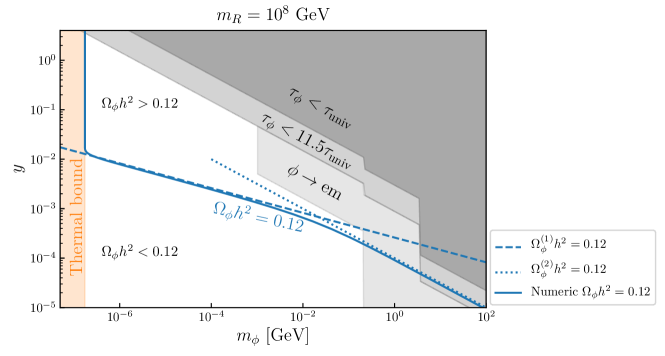
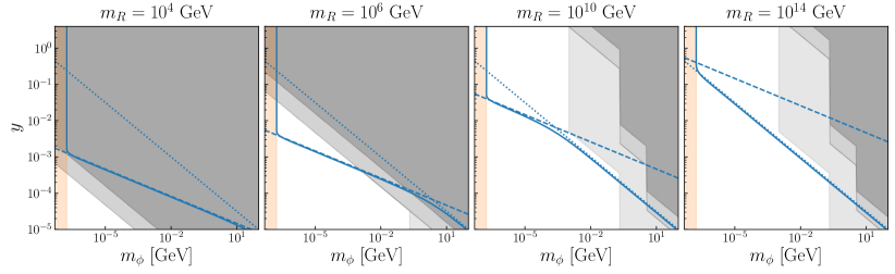
Figure 2: Upper panel: the parameter space of the $\nu_{R}$-philic scalar DM, assuming $m_{R}=10^{8}$ GeV. The blue solid curve leads to the observed DM relic abundance, $\Omega_{\phi}h^{2}=0.12$, obtained by numerically solving the Boltzmann equation. The dashed and dotted lines take into account only the contributions of $2\nu_{R}\to 2\phi$ and $LH\to\nu_{R}\phi$, obtained using Eqs. (3.10) and (3.16), respectively. The gray shaded regions correspond to $\tau_{\phi}<\tau_{{\rm univ}}$ (darkest gray region), $\tau_{\phi}<11.5\ \tau_{{\rm univ}}$ (lighter gray region), and $\tau_{\phi\to{\rm em}}<10^{25}\ \text{s}$ (lightest gray region). The thermal bound (orange) applies to DM candidates that are produced via thermal processes above the electroweak scale—see Eq. (3.13). Lower panels: similar to the upper panel but with different values of $m_{R}$. The color coding is the same as the upper panel.

In our model, there are only three relevant free parameters: the coupling $y$ and the two masses $m_{\phi}$ and $m_{R}$. The seesaw Yukawa coupling $y_{\nu}$ is essentially determined by $m_{R}$ via the seesaw relation in Eq. (2.3). Therefore, a convenient way to explore the parameter space is to fix $m_{R}$ (consequently, $y_{\nu}=\sqrt{2m_{\nu}m_{R}}/v$ is also fixed) and vary $m_{\phi}$ and $y$.

We are mainly concerned with two constraints: (i) large $y$ and $m_{\phi}$ may render the lifetime of $\phi$ too short; and (ii) large $y$ may bring $\phi$ into thermal equilibrium and, in the absence of freeze-out suppression, may potentially lead to an overproduction of $\Omega_{\phi}h^{2}$.

For constraint (i), we include the dominant decay widths calculated in Sec. 3.1 and compare the obtained lifetime with the age of the universe, $\tau_{{\rm univ}}\approx 4.35\times 10^{17}\ \text{s}$ ($13.79\times 10^{9}$ yr). This is presented in Fig. 2, where the darkest gray region corresponds to $\tau_{\phi}<\tau_{{\rm univ}}$. One should note, however, that this is only a conservative theoretical bound. When being confronted with observational data, $\tau_{\phi}$ actually needs to be much larger than $\tau_{{\rm univ}}$. The specific bounds depend on whether $\phi$ decays to invisible radiations (e.g. $\nu_{L}$) or electromagnetic channels (e.g. $e^{\pm}$, $\mu^{\pm}$, $\tau^{\pm}$, $\gamma$). For the former, the latest bound is $\tau_{\phi}^{-1}<6.3\times 10^{-3}\ \text{Gyr}^{-1}$ Poulin:2016nat , corresponding to $\tau_{\phi}>11.5\ \tau_{{\rm univ}}$, which is shown in Fig. 2 as the lighter gray region. For the latter, the bounds depend on the ionization efficiency of the decay Zhang:2007zzh . For instance, $\nu_{L}$ from $\phi$ decay or from the subsequent decay of $\mu^{\pm}$ and $\tau^{\pm}$ cannot contribute to the ionization energy. If the decay energy is fully converted to the ionization energy, then the decay width $\Gamma_{\phi\to\text{em}}$ should be below $10^{-25}\ \text{s}^{-1}$ Poulin:2016anj . We apply this bound to the partial decay width of $\phi\to 2\ell$ and present it in Fig. 2 as the lightest gray region.

For constraint (ii), since the dominant processes for $\phi$ production is efficient only at temperatures above the electroweak scale while the decay is significant only at a time scale much larger than $\tau_{{\rm univ}}$, we assume that $n_{\phi}a^{3}$ remains constant during the period from $T\sim{\cal O}(10^{2})$ GeV to today. Note that the maximum of $n_{\phi}a^{3}$ is $n_{\phi}^{{\rm eq}}a^{3}=\frac{\zeta(3)}{\pi^{2}}T^{3}a^{3}$ according to Eq. (2.6). The corresponding maximal value of $n_{\phi}$ today then implies a lower bound on $m_{\phi}$ according to Eq. (2.7). This bound is given by Eq. (3.13) and indicated as the thermal bound in Fig. 2.

In the upper panel of Fig. 2, we fix $m_{R}$ at $10^{8}$ GeV and plot the blue dashed and dotted lines by requiring that $\Omega_{\phi}^{(1)}h^{2}$ in Eq. (3.10) and $\Omega_{\phi}^{(2)}h^{2}$ in Eq. (3.16) reach the observed DM relic abundance. The solid line is obtained by numerically solving the Boltzmann equation, which will be detailed in Sec. 4.

In the lower panels, we present similar plots for $m_{R}=10^{4}$, $10^{6}$, $10^{10}$, and $10^{14}$ GeV. As is shown here, lighter $\nu_{R}$ leads to more constrained parameter space to accommodate a viable DM candidate. The main reason for this is that smaller $m_{R}$ implies larger $\nu_{L}$-$\nu_{R}$ mixing and hence higher decay rate of $\phi\to 2\nu_{L}$. By requiring that $\Gamma_{\phi\to 2\nu_{L}}$ is below $\tau_{{\rm univ}}^{-1}$ or $(11.5\tau_{{\rm univ}})^{-1}$ and using the lower bound in Eq. (3.13), we obtain

$$m_{R}\gtrsim\begin{cases}1.1\times 10^{4}\ \text{GeV}\thinspace&\text{for }\Gamma_{\phi\to 2\nu_{L}}<\tau_{{\rm univ}}^{-1}\\ 5.5\times 10^{4}\ \text{GeV}\thinspace&\text{for }\Gamma_{\phi\to 2\nu_{L}}<(11.5\tau_{{\rm univ}})^{-1}\end{cases},$$ (3.20)

which can be taken as the lower bound on $m_{R}$ if $\phi$ is to be considered as DM.

4 Solving the Boltzmann equation

Our analytical results in Eqs. (3.10) and (3.16) are derived using the freeze-in formalism, which is valid only when the depletion term in the Boltzmann equation is negligible. For relatively large $y$ or $y_{\nu}$, the depletion term needs to be taken into account and one needs to solve the Boltzmann equation to obtain accurate results.

To solve the Boltzmann equation numerically, we rewrite Eq. (3.15) as follows

$$\frac{d\left(n_{\phi}a^{3}\right)}{da}=\frac{a^{2}}{H}\left(C_{\text{prod}}-C_{\text{depl}}\right).$$ (4.1)

For the production term $C_{\text{prod}}$, we include contributions from the two dominant processes, $2\nu_{R}\to 2\phi$ and $LH\to\nu_{R}\phi$. The depletion term $C_{\text{depl}}$, caused by the backreactions $2\phi\to 2\nu_{R}$ and $\nu_{R}\phi\to LH$, would be equal to $C_{\text{prod}}$ if $\phi$ reaches thermal equilibrium with the thermal bath. Here we assume that $\phi$ is able to maintain internal equilibrium with itself such that it has a well-defined temperature $T_{\phi}$, which can be computed from $n_{\phi}$. Under this assumption, $C_{\text{depl}}$ can be computed by replacing $T$ in $C_{\text{prod}}$ with $T_{\phi}$.

With the above setup, it is straightforward to solve the Boltzmann equation numerically. Fig. 3 shows an example with $m_{R}=10^{8}$ GeV, $m_{\phi}=10^{-4}$ GeV, and $y=3\times 10^{-4}$. In addition to the full numerical solution (blue solid line), we also split it into two contributions $2\nu_{R}\to 2\phi$ and $LH\to\nu_{R}\phi$, presented by the dashed and dotted curves there. This example illustrates the possibility of a scenario where the process $2\nu_{R}\to 2\phi$ predominates in the initial stage, with $LH\to\phi\nu_{R}$ taking over as the dominant process at a later phase.

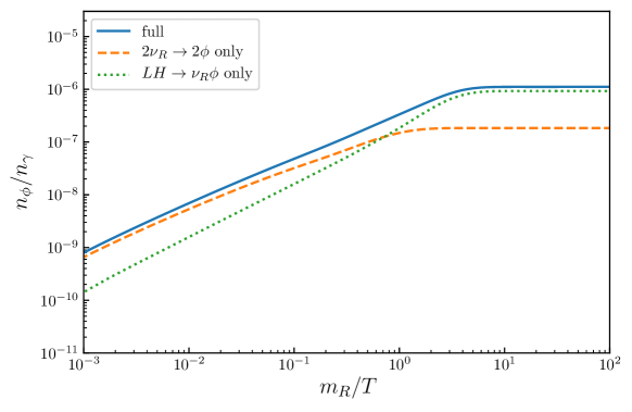
Figure 3: Numerical solutions of the Boltzmann equation, with $m_{R}=10^{8}$ GeV, $m_{\phi}=10^{-4}$ GeV, and $y=3\times 10^{-4}$. The solid curve represent the full numerical solution while the dashed and dotted lines represents the contributions of $2\nu_{R}\to 2\phi$ and $LH\to\phi\nu_{R}$.

As mentioned above, large $y$ would lead to the invalidity of the freeze-in formalism since $C_{\text{depl}}$ becomes significant. Indeed, the blue solid curves in Fig. 2 obtained from numerical solutions exhibit turning points when they approach the orange region. Above the turning points, $\Omega_{\phi}h^{2}$ becomes independent of $y$ due to the established equilibrium between $\phi$ and the thermal bath.

5 Neutrino signals from DM

As a decaying DM candidate, the $\nu_{R}$-philic scalar features interesting neutrino signals for DM indirect detection. Indeed, in the low-mass regime with $m_{\phi}<2m_{\mu}\approx 212$ MeV and $m_{R}<1.5\times 10^{10}\ \text{GeV}$ [see Eq. (3.4)], its dominant decay channel is $\phi\to 2\nu_{L}$, implying the emission of monochromatic neutrino lines, which if detected would be a smoking-gun signal for DM indirect detection.

Neutrino signals as a novel approach to DM indirect detection have been investigated in a number of studies Palomares-Ruiz:2007egs ; Dudas:2014bca ; Garcia-Cely:2017oco ; Coy:2020wxp ; Coy:2021sse ; Hufnagel:2021pso . A crucial difference between the neutrino signals in our model and in various previously considered scenarios is that heavy DM with $m_{\phi}$ above $2m_{\mu}$ in our model has been ruled out—see Fig. 2. Consequently, the neutrino signals are less energetic and the observation of high-energy astrophysical neutrinos at IceCube, ANTARES, and other neutrino telescopes cannot be used in our model. At low energies, searches for extraterrestrial neutrinos have been conducted by Super-Kamiokande (SK) Super-Kamiokande:2002exp ; Super-Kamiokande:2013ufi , Borexino Borexino:2010zht , and KamLAND KamLAND:2011bnd , adopting inverse beta decay (IBD, $\overline{\nu}_{e}+p\to n+e^{+}$) as the primary detection channel due to its relatively low-background, large cross section, and successful event identification.

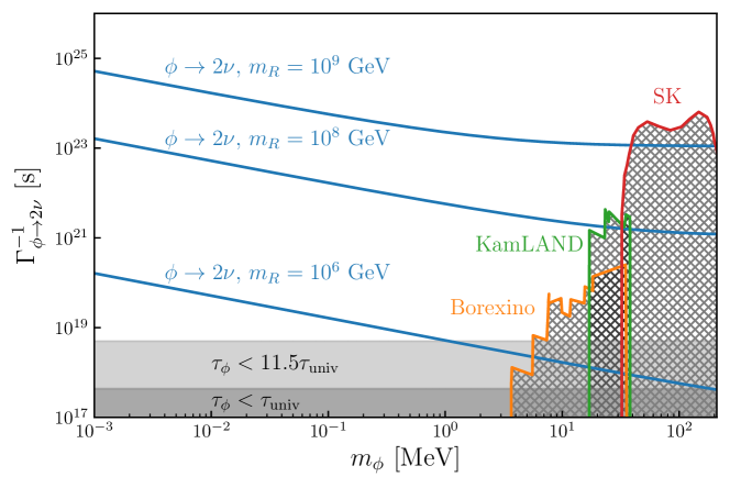
Figure 4: The strength of neutrino signals (blue lines) from $\phi$ decay compared with experimental limits (hatched regions) from SK Super-Kamiokande:2002exp ; Super-Kamiokande:2013ufi , Borexino Borexino:2010zht , and KamLAND KamLAND:2011bnd —see Refs. Palomares-Ruiz:2007egs ; Garcia-Cely:2017oco for compilations of these limits.

In our framework, the decay width of the $\nu_{R}$-philic scalar DM is determined by $\Omega_{\phi}h^{2}=0.12$, if $m_{R}$ and $m_{\phi}$ are fixed at given values. In Fig. 4, we plot the decay width of $\phi\to 2\nu_{L}$ as a function of $m_{\phi}$ for $m_{R}=10^{6}$, $10^{8}$ and $10^{9}$ GeV. This is to be confronted with the limits reached by the aforementioned neutrino experiments. Here we assume that $\phi$ predominantly decays to $\overline{\nu}_{e}$, since the experimental searches are conducted in the IBD channel. It is possible that, by tuning the flavor structure in the neutrino sector, one obtains a suppressed branching ratio of $\phi$ to $\overline{\nu}_{e}$. For example, $\phi$ may predominantly decay to $\nu_{\tau}$. In this case, the experimental sensitivity would be substantially reduced. We leave a more dedicated analysis involving the flavor structure to future work.

6 Conclusion

In this study, we explore a simple extension of the Type-I seesaw model, in which a real scalar $\phi$ is introduced and exclusively coupled to right-handed neutrinos $\nu_{R}$, hence referred to as the $\nu_{R}$-philic scalar. Our primary objective is to assess whether the $\nu_{R}$-philic scalar can serve as a viable DM candidate while preserving the success of Type-I seesaw in explaining the small neutrino masses. To this end, we systematically investigate the decay channels of the $\nu_{R}$-philic scalar, compute the thermal production rates of $\phi$, and, by combining the results regarding these two aspects, obtain the viable parameter space for $\phi$ to qualify as DM.

The viable parameter space is presented in Fig. 2. Notably, this parameter space necessitates that the scalar mass should be above $173.4$ eV and below 212 MeV (i.e. $2m_{\mu}$) for $\phi$ to be DM. Moreover, our research underlines the critical role played by the mass of $\nu_{R}$ in shaping this parameter space. A lighter $\nu_{R}$ leads to larger $\nu_{L}$-$\nu_{R}$ mixing and increases the decay width of $\phi\to 2\nu_{L}$, resulting more constrained parameter space. According to Eq. (3.20), the viable parameter space sets a lower bound of $\sim 10^{4}$ GeV for the $\nu_{R}$ mass.

Further, we consider the observational consequence of the $\nu_{R}$-philic scalar DM within the viable parameter space. The emission of monochromatic neutrino lines from $\phi$ decay, if detected, would be a smoking-gun signal for DM indirect detection. In our model, the neutrino lines are less energetic than $\sim 10^{2}$ MeV and cannot contribute to the observation of high-energy astrophysical neutrinos at IceCube. Within the energy range from a few to $\sim 10^{2}$ MeV, they could be detected by the present neutrino detectors.

In summary, our investigation provides a comprehensive exploration of the $\nu_{R}$-philic scalar as a DM candidate, shedding light on the interplay between neutrinos and DM. The constraints we have identified regarding the masses of $\phi$ and $\nu_{R}$ constitute a valuable foundation for forthcoming experimental and theoretical explorations aimed at deciphering the enigmatic nature of DM and its connections to a broader landscape of particle physics.

Appendix A Squared amplitudes, cross sections, and collision terms

In this appendix, we present detailed calculations of squared amplitudes, cross sections, and collision terms used in this work. Regarding the Majorana feature of $\nu_{R}$, although the two-component notation of Weyl spinors is conceptually simple, it is more convenient to adopt four-component spinors due to well-developed computing packages. Hence we rewrite the $\nu_{R}\nu_{R}\phi$ term in Eq. (2.1) in terms of Majorana spinors:

$$\mathcal{L}\supset\frac{y}{2}\overline{\Psi}_{M}\phi\Psi_{M}\thinspace,\ \ \Psi_{M}\equiv\left(\begin{array}[]{c}\nu_{R}\\[5.69054pt] \nu_{R}^{\dagger}\end{array}\right).$$ (A.1)

Note that, unlike Eq. (2.1), here we do not add an “h.c.” term because $y$ is real. If $y$ were complex, then the Lagrangian would be $\mathcal{L}\supset\frac{1}{2}\overline{\Psi}_{M}(yP_{L}+y^{*}P_{R})\phi\Psi_{M}$.

A.1 $2\nu_{R}\rightarrow 2\phi$

Since $\phi$ is a real scalar, there are two diagrams contributing to this process, the $t$-channel and $u$-channel diagrams. Including the two channels, the scattering amplitude of $2\nu_{R}\rightarrow 2\phi$ reads:

$$i{\cal M}_{2\nu_{R}\rightarrow 2\phi}=-iy^{2}\overline{v}_{2}\frac{\not{q}_{1}+m_{R}}{t-m_{R}^{2}}u_{1}-iy^{2}\overline{v}_{2}\frac{\not{q}_{2}+m_{R}}{u-m_{R}^{2}}u_{1}\thinspace,$$ (A.2)

where $\overline{\nu}_{2}$ and $u_{1}$ denote the two initial state of $\nu_{R}$, and $q_{1}(q_{2})$ is the momentum of the $t$($u$)-channel propagator. Hence, $t=q_{1}^{2}$ and $u=q_{2}^{2}$. After applying the standard procedure of computing traces, we get

$$|{\cal M}_{2\nu_{R}\rightarrow 2\phi}|^{2} =2y^{4}\frac{tu\left(t-u\right)^{2}-m_{R}^{2}\left(t+u\right)\left(t^{2}+14tu+u^{2}\right)}{\left(t-m_{R}^{2}\right)^{2}\left(u-m_{R}^{2}\right)^{2}}$$

$$\phantom{=}+2y^{4}\frac{m_{R}^{4}\left(t^{2}+30tu+u^{2}\right)+16m_{R}^{6}\left(t+u\right)-32m_{R}^{8}}{\left(t-m_{R}^{2}\right)^{2}\left(u-m_{R}^{2}\right)^{2}}\thinspace.$$ (A.3)

The cross section of $2\nu_{R}\rightarrow 2\phi$ in the center-of-mass frame is

$$\sigma_{2\nu_{R}\rightarrow 2\phi} =\frac{1}{S}\int\frac{\beta_{f}|{\cal M}_{2\nu_{R}\rightarrow 2\phi}|^{2}}{64\pi^{2}s\beta_{i}}d\Omega$$ (A.4)

$$=\frac{y^{4}}{4\pi s\beta_{i}^{2}}\left(2\beta_{i}^{3}-3\beta_{i}+\left(3-2\beta_{i}^{4}\right)\tanh^{-1}\beta_{i}\right),$$

where $\beta_{i}$ and $\beta_{f}$ denote the velocities of the initial and final particles, and $S=2$ is the symmetry factor due to identical particles. In the above calculation, we have assumed $m_{R}\gg m_{\phi}$ so that $\beta_{f}\approx 1$.

The collision term can be computed by further integrating the cross section Gondolo:1990dk :

$$C_{2\nu_{R}\rightarrow 2\phi}\approx\frac{TN_{f}}{32\pi^{4}}\int_{4m_{R}^{2}}^{\infty}s^{\frac{1}{2}}(s-4m_{R}^{2})\sigma_{2\nu_{R}\rightarrow 2\phi}K_{1}\left(\frac{\sqrt{s}}{T}\right)ds\thinspace.$$ (A.5)

Analytically, the integral can only be computed in the low-$T$ ($T\ll m_{R}$) and high-$T$ ($T\gg m_{R}$) limits.

In the low-$T$ limit, $\beta_{i}\rightarrow 0$, we can expand $\tanh^{-1}\beta_{i}$ in terms of polynomial of $\beta_{i}$. The leading order gives

$$\sigma_{2\nu_{R}\rightarrow 2\phi}\approx\frac{3y^{4}\beta_{i}}{4\pi s}\thinspace.$$ (A.6)

Substituting Eq. (A.6) into Eq. (A.5), we obtain

$$C_{2\nu_{R}\rightarrow 2\phi}\approx\frac{9y^{4}N_{f}}{128\pi^{4}}T^{4}e^{-2m_{R}/T}\thinspace.$$ (A.7)

As for the high-$T$ limit, we can expand the cross section $\sigma_{2\nu_{R}\rightarrow 2\phi}$ in terms of $m_{R}$. Neglecting terms of ${\cal O}(m_{R}^{2})$, we obtain

$$\sigma_{2\nu_{R}\rightarrow 2\phi}\approx\frac{y^{4}}{8\pi s}\left[\ln\left(\frac{s}{m_{R}^{2}}\right)-2\right].$$ (A.8)

Substituting Eq. (A.8) into Eq. (A.5) and assuming $\ln(T/m_{R})\gg 1$, we obtain

$$C_{2\nu_{R}\rightarrow 2\phi}\approx\frac{y^{4}N_{f}}{32\pi^{5}}T^{4}\ln\left(\frac{2T}{m_{R}}\right).$$ (A.9)

Based on Eqs. (A.7) and (A.9), one can construct an analytical expression that approaches Eqs. (A.7) and (A.9) in the low-$T$ and high-$T$ limits. The expression is presented in Eq. (3.7).

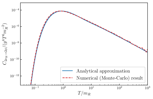
Figure 5: Analytical approximation of the collision term $C_{2\nu_{R}\to 2\phi}$ [given in Eq. (3.7)] compared with the numerical result obtained using the Monte-Carlo method.

Let us compare our analytical result with the numerical result obtained by directly evaluating the following integral:

$$C_{2\nu_{R}\to 2\phi}=N_{f}\int d\Pi_{1}d\Pi_{2}d\Pi_{3}d\Pi_{4}f_{\nu_{R}}^{2}|{\cal M}_{2\nu_{R}\rightarrow 2\phi}|^{2}(2\pi)^{4}\delta^{4}\thinspace,$$ (A.10)

where $d\Pi_{i}\equiv\frac{d^{3}\mathbf{p}_{i}}{2E_{i}(2\pi)^{3}}$ with $i$ indicating the $i$-th particles in the process $\nu_{R}+\nu_{R}\rightarrow\phi+\phi$. The momentum distribution function $f_{\nu_{R}}$ takes the Fermi-Dirac distribution. We adopt the Monte-Carlo method introduced in Appendix B of Ref. Luo:2020fdt to perform the integration. Fig. 5 shows the comparison of the analytical expression in Eq. (3.7) with the numerical result. Obviously, Eq. (3.7) is quite accurate when compared with the numerical result.

A.2 $LH\rightarrow\nu_{R}\phi$

In the main text of this paper, $LH\rightarrow\nu_{R}\phi$ actually refers to two processes, $LH\rightarrow\nu_{R}\phi$ and its antiparticle companion, $\overline{L}\overline{H}\rightarrow\nu_{R}\phi$.

For $LH\rightarrow\nu_{R}\phi$, the scattering amplitude reads:

$$i{\cal M}_{LH\rightarrow\nu_{R}\phi}=-i\frac{yy_{\nu}}{s-m_{R}^{2}}\overline{u}_{3}\left(\not{p}+m_{R}\right)P_{L}u_{1}\thinspace,$$

where $\overline{u}_{3}$ and $u_{1}$ denote the final state of $\nu_{R}$ and the initial state of $L$, respectively. The momentum of the $s$-channel propagator in this process is denoted by $p$, with $s=p^{2}$.

The squared amplitude is then given by

$$|{\cal M}_{LH\rightarrow\nu_{R}\phi}|^{2} =\frac{y^{2}y_{\nu}^{2}}{\left(s-m_{R}^{2}\right)^{2}}\text{Tr}\left[\left(\not{p}_{3}+m_{R}\right)\left(\not{p}+m_{R}\right)P_{L}\not{p}_{1}P_{R}\left(\not{p}+m_{R}\right)\right]$$ (A.11)

$$=\frac{y^{2}y_{\nu}^{2}\left(m_{R}^{4}+m_{R}^{2}\left(3s-t\right)-su\right)}{\left(s-m_{R}^{2}\right)^{2}}\thinspace,$$

where we have neglected all particle masses except for $m_{R}$.

Note that $L$ and $H$ are electroweak $SU(2)$ doublets. In this regard, we interpret the above result as the squared amplitude of each component of $L$ scattering off the corresponding component of $H$. For cross sections presented below, we also adopt the same convention. The combined contribution of the two $SU(2)$ components in $L$ (i.e. $\nu_{L}$ and $e_{L}$), together with the contribution of the antiparticle channel ($\overline{L}\overline{H}\rightarrow\nu_{R}\phi$), will be summed in the final result of the collision term.

Integrating the squared amplitude, we obtain the cross section

$$\sigma_{LH\rightarrow\nu_{R}\phi}=\frac{y^{2}y_{\nu}^{2}}{32\pi s^{2}}\cdot\frac{m_{R}^{4}+6m_{R}^{2}s+s^{2}}{s-m_{R}^{2}}\thinspace.$$ (A.12)

For $\overline{L}\overline{H}\rightarrow\nu_{R}\phi$, the scattering amplitude reads:

$$i{\cal M}_{\overline{L}\overline{H}\rightarrow\nu_{R}\phi}=-i\frac{yy_{\nu}}{s-m_{R}^{2}}\overline{v}_{1}\left(\not{p}+m_{R}\right)P_{R}v_{3}\thinspace,$$ (A.13)

where $\overline{v}_{1}$ and $v_{3}$ denote the initial state of $L$ and the final state of $\nu_{R}$, respectively.

Correspondingly, the squared amplitude is

$$|{\cal M}_{\overline{L}\overline{H}\rightarrow\nu_{R}\phi}|^{2} =\frac{y^{2}y_{\nu}^{2}}{\left(s-m_{R}^{2}\right)^{2}}\text{Tr}\left[\not{p}_{1}\left(\not{p}+m_{R}\right)P_{R}\left(\not{p}_{3}-m_{R}\right)P_{L}\left(\not{p}+m_{R}\right)\right]$$ (A.14)

$$=\frac{yy_{\nu}^{2}\left(m_{R}^{4}+m_{R}^{2}\left(s-t\right)-su\right)}{\left(s-m_{R}^{2}\right)^{2}}\thinspace,$$

which leads to the following cross section

$$\sigma_{\overline{L}\overline{H}\rightarrow\nu_{R}\phi}=\frac{y^{2}y_{\nu}^{2}}{32\pi s^{2}}\cdot\frac{\left(s+m_{R}^{2}\right)^{2}}{s-m_{R}^{2}}.$$ (A.15)

We see that in the high-energy limit, $s\gg m_{R}$, Eqs. (A.12) and (A.15) lead to the same result

$$\lim_{s\to\infty}\sigma_{LH\rightarrow\nu_{R}\phi}=\lim_{s\to\infty}\sigma_{\overline{L}\overline{H}\rightarrow\nu_{R}\phi}=\frac{y^{2}y_{\nu}^{2}}{32\pi s}\thinspace,$$ (A.16)

while in the low-energy limit, $s-m_{R}^{2}\equiv\delta\to 0$, Eqs. (A.12) and (A.15) differ by a factor of two:

$$\lim_{s\to m_{R}^{2}}\sigma_{LH\rightarrow\nu_{R}\phi}=\frac{y^{2}y_{\nu}^{2}}{4\pi\delta}\thinspace,\ \ \lim_{s\to m_{R}^{2}}\sigma_{\overline{L}\overline{H}\rightarrow\nu_{R}\phi}=\frac{y^{2}y_{\nu}^{2}}{8\pi\delta}\thinspace.$$ (A.17)

The collision term responsible for the production of $\phi$ via the above two processes, including the independent contributions from the $\nu_{L}$ and $e_{L}$ components in $L$, is computed by

$$C_{LH\rightarrow\nu_{R}\phi}\approx\frac{TN_{f}}{32\pi^{4}}\int_{m_{R}^{2}}^{\infty}\left(2\sigma_{LH\rightarrow\nu_{R}\phi}+2\sigma_{\overline{L}\overline{H}\rightarrow\nu_{R}\phi}\right)s^{1/2}\left(s-m_{R}^{2}\right)K_{1}\left(\frac{\sqrt{s}}{T}\right)ds\thinspace.$$ (A.18)

At high temperatures, we substitute Eq. (A.16) into Eq. (A.18) and obtain

$$C_{LH\rightarrow\nu_{R}\phi} \approx\frac{y^{2}y_{\nu}^{2}N_{f}}{64\pi^{5}}m_{R}T^{3}K_{1}\left(\frac{m_{R}}{T}\right)$$ (A.19)

$$\approx\frac{y^{2}y_{\nu}^{2}N_{f}}{64\pi^{5}}T^{4}\thinspace,\ \ \ (T\gg m_{R})\thinspace.$$ (A.20)

At low temperatures, we substitute Eq. (A.17) into Eq. (A.18) and obtain

$$C_{LH\rightarrow\nu_{R}\phi} \approx\frac{y^{2}y_{\nu}^{2}N_{f}}{64\pi^{5}}3m_{R}^{2}T^{2}K_{2}\left(\frac{m_{R}}{T}\right),\ \ \ \ \ \ (T\ll m_{R})\thinspace.$$ (A.21)

Since $\lim_{x\to 0}K_{1}\left(x\right)/K_{2}\left(x\right)=x/2$, we propose the following expression that can cover both the high-$T$ and low-$T$ limits:

$$C_{LH\rightarrow\nu_{R}\phi} \approx\frac{y^{2}y_{\nu}^{2}N_{f}}{64\pi^{5}}3m_{R}^{2}T^{2}K_{2}\left(\frac{m_{R}}{T}\right)\frac{m_{R}^{2}+T^{2}}{m_{R}^{2}+6T^{2}}\thinspace.$$ (A.22)

As we have checked, when compared to numerical results from the Monte-Carlo integration, Eq. (A.22) also exhibits excellent accuracy.

- (1) B. Dasgupta and J. Kopp, Sterile neutrinos, Phys. Rept. 928 (2021) 1–63, [2106.05913].
- (2) K. N. Abazajian, Sterile neutrinos in cosmology, Phys. Rept. 711-712 (2017) 1–28, [1705.01837].
- (3) M. Drewes et al., A White Paper on keV Sterile Neutrino Dark Matter, JCAP 01 (2017) 025, [1602.04816].
- (4) S. Dodelson and L. M. Widrow, Sterile-neutrinos as dark matter, Phys. Rev. Lett. 72 (1994) 17–20, [hep-ph/9303287].
- (5) N. Palanque-Delabrouille, C. Yèche, N. Schöneberg, J. Lesgourgues, M. Walther, S. Chabanier, and E. Armengaud, Hints, neutrino bounds and WDM constraints from SDSS DR14 Lyman- and Planck full-survey data, JCAP 04 (2020) 038, [1911.09073].
- (6) M. Pospelov, A. Ritz, and M. B. Voloshin, Secluded WIMP Dark Matter, Phys. Lett. B 662 (2008) 53–61, [0711.4866].
- (7) A. Falkowski, J. Juknevich, and J. Shelton, Dark Matter Through the Neutrino Portal, 0908.1790.
- (8) V. González-Macías, J. I. Illana, and J. Wudka, A realistic model for Dark Matter interactions in the neutrino portal paradigm, JHEP 05 (2016) 171, [1601.05051].
- (9) M. Escudero, N. Rius, and V. Sanz, Sterile Neutrino portal to Dark Matter II: Exact Dark symmetry, Eur. Phys. J. C 77 (2017), no. 6 397, [1607.02373].
- (10) Y.-L. Tang and S.-h. Zhu, Dark Matter Relic Abundance and Light Sterile Neutrinos, JHEP 01 (2017) 025, [1609.07841].
- (11) B. Batell, T. Han, and B. Shams Es Haghi, Indirect Detection of Neutrino Portal Dark Matter, Phys. Rev. D 97 (2018), no. 9 095020, [1704.08708].
- (12) P. Bandyopadhyay, E. J. Chun, R. Mandal, and F. S. Queiroz, Scrutinizing Right-Handed Neutrino Portal Dark Matter With Yukawa Effect, Phys. Lett. B 788 (2019) 530–534, [1807.05122].
- (13) M. Becker, Dark Matter from Freeze-In via the Neutrino Portal, Eur. Phys. J. C 79 (2019), no. 7 611, [1806.08579].
- (14) M. Chianese and S. F. King, The Dark Side of the Littlest Seesaw: freeze-in, the two right-handed neutrino portal and leptogenesis-friendly fimpzillas, JCAP 09 (2018) 027, [1806.10606].
- (15) M. G. Folgado, G. A. Gómez-Vargas, N. Rius, and R. Ruiz De Austri, Probing the sterile neutrino portal to Dark Matter with rays, JCAP 08 (2018) 002, [1803.08934].
- (16) M. Chianese, B. Fu, and S. F. King, Minimal Seesaw extension for Neutrino Mass and Mixing, Leptogenesis and Dark Matter: FIMPzillas through the Right-Handed Neutrino Portal, JCAP 03 (2020) 030, [1910.12916].
- (17) E. Hall, T. Konstandin, R. McGehee, and H. Murayama, Asymmetric matter from a dark first-order phase transition, Phys. Rev. D 107 (2023), no. 5 055011, [1911.12342].
- (18) M. Blennow, E. Fernandez-Martinez, A. Olivares-Del Campo, S. Pascoli, S. Rosauro-Alcaraz, and A. V. Titov, Neutrino Portals to Dark Matter, Eur. Phys. J. C 79 (2019), no. 7 555, [1903.00006].
- (19) P. Bandyopadhyay, E. J. Chun, and R. Mandal, Feeble neutrino portal dark matter at neutrino detectors, JCAP 08 (2020) 019, [2005.13933].
- (20) E. Hall, R. McGehee, H. Murayama, and B. Suter, Asymmetric dark matter may not be light, Phys. Rev. D 106 (2022), no. 7 075008, [2107.03398].
- (21) M. Chianese, B. Fu, and S. F. King, Dark Matter in the Type Ib Seesaw Model, JHEP 05 (2021) 129, [2102.07780].
- (22) A. Biswas, D. Borah, and D. Nanda, Light Dirac neutrino portal dark matter with observable Neff, JCAP 10 (2021) 002, [2103.05648].
- (23) R. Coy, A. Gupta, and T. Hambye, Seesaw neutrino determination of the dark matter relic density, Phys. Rev. D 104 (2021), no. 8 083024, [2104.00042].
- (24) R. Coy and A. Gupta, A closer look at the seesaw-dark matter correspondence, JCAP 02 (2023) 028, [2211.05091].
- (25) B. Barman, P. S. Bhupal Dev, and A. Ghoshal, Probing freeze-in dark matter via heavy neutrino portal, Phys. Rev. D 108 (2023), no. 3 035037, [2210.07739].
- (26) L. Coito, C. Faubel, J. Herrero-García, A. Santamaria, and A. Titov, Sterile neutrino portals to Majorana dark matter: effective operators and UV completions, JHEP 08 (2022) 085, [2203.01946].
- (27) S.-P. Li and X.-J. Xu, Dark matter produced from right-handed neutrinos, JCAP 06 (2023) 047, [2212.09109].
- (28) E. Dudas, Y. Mambrini, and K. A. Olive, Monochromatic neutrinos generated by dark matter and the seesaw mechanism, Phys. Rev. D 91 (2015) 075001, [1412.3459].
- (29) S.-P. Li and B. Yu, A cosmological sandwiched window for seesaw with primordial majoron abundance, 2310.13492.
- (30) V. Berezinsky and J. W. F. Valle, The KeV majoron as a dark matter particle, Phys. Lett. B 318 (1993) 360–366, [hep-ph/9309214].
- (31) F. Bazzocchi, M. Lattanzi, S. Riemer-Sørensen, and J. W. F. Valle, X-ray photons from late-decaying majoron dark matter, JCAP 08 (2008) 013, [0805.2372].
- (32) P.-H. Gu, E. Ma, and U. Sarkar, Pseudo-Majoron as Dark Matter, Phys. Lett. B 690 (2010) 145–148, [1004.1919].
- (33) M. Frigerio, T. Hambye, and E. Masso, Sub-GeV dark matter as pseudo-Goldstone from the seesaw scale, Phys. Rev. X 1 (2011) 021026, [1107.4564].
- (34) M. Lattanzi, S. Riemer-Sorensen, M. Tortola, and J. W. F. Valle, Updated CMB and x- and -ray constraints on Majoron dark matter, Phys. Rev. D 88 (2013), no. 6 063528, [1303.4685].
- (35) F. S. Queiroz and K. Sinha, The Poker Face of the Majoron Dark Matter Model: LUX to keV Line, Phys. Lett. B 735 (2014) 69–74, [1404.1400].
- (36) S. M. Boucenna, S. Morisi, Q. Shafi, and J. W. F. Valle, Inflation and majoron dark matter in the seesaw mechanism, Phys. Rev. D 90 (2014), no. 5 055023, [1404.3198].
- (37) C. Garcia-Cely and J. Heeck, Neutrino Lines from Majoron Dark Matter, JHEP 05 (2017) 102, [1701.07209].
- (38) M. Reig, J. W. F. Valle, and M. Yamada, Light majoron cold dark matter from topological defects and the formation of boson stars, JCAP 09 (2019) 029, [1905.01287].
- (39) K. Akita and M. Niibo, Updated constraints and future prospects on majoron dark matter, JHEP 07 (2023) 132, [2304.04430].
- (40) Y. Chikashige, R. N. Mohapatra, and R. D. Peccei, Are There Real Goldstone Bosons Associated with Broken Lepton Number?, Phys. Lett. B 98 (1981) 265–268.
- (41) H. K. Dreiner, H. E. Haber, and S. P. Martin, Two-component spinor techniques and Feynman rules for quantum field theory and supersymmetry, Phys. Rept. 494 (2010) 1–196, [0812.1594].
- (42) X.-J. Xu, The -philic scalar: its loop-induced interactions and Yukawa forces in LIGO observations, JHEP 09 (2020) 105, [2007.01893].
- (43) G. Chauhan and X.-J. Xu, How dark is the -philic dark photon?, JHEP 04 (2021) 003, [2012.09980].
- (44) G. Chauhan, P. S. B. Dev, and X.-J. Xu, Probing the R-philic Z’ at DUNE near detectors, Phys. Lett. B 841 (2023) 137907, [2204.11876].
- (45) W. Buchmuller, P. Di Bari, and M. Plumacher, Leptogenesis for pedestrians, Annals Phys. 315 (2005) 305–351, [hep-ph/0401240].
- (46) X. Luo, W. Rodejohann, and X.-J. Xu, Dirac neutrinos and Neff. Part II. The freeze-in case, JCAP 03 (2021) 082, [2011.13059].
- (47) M. Escudero Abenza, Precision early universe thermodynamics made simple: and neutrino decoupling in the Standard Model and beyond, JCAP 05 (2020) 048, [2001.04466].
- (48) X. Luo, W. Rodejohann, and X.-J. Xu, Dirac neutrinos and , JCAP 06 (2020) 058, [2005.01629].
- (49) V. Poulin, P. D. Serpico, and J. Lesgourgues, A fresh look at linear cosmological constraints on a decaying dark matter component, JCAP 08 (2016) 036, [1606.02073].
- (50) L. Zhang, X. Chen, M. Kamionkowski, Z.-g. Si, and Z. Zheng, Constraints on radiative dark-matter decay from the cosmic microwave background, Phys. Rev. D 76 (2007) 061301, [0704.2444].
- (51) V. Poulin, J. Lesgourgues, and P. D. Serpico, Cosmological constraints on exotic injection of electromagnetic energy, JCAP 03 (2017) 043, [1610.10051].
- (52) S. Palomares-Ruiz, Model-independent bound on the dark matter lifetime, Phys. Lett. B 665 (2008) 50–53, [0712.1937].
- (53) R. Coy and T. Hambye, Neutrino lines from DM decay induced by high-scale seesaw interactions, JHEP 05 (2021) 101, [2012.05276].
- (54) M. Hufnagel and X.-J. Xu, Dark matter produced from neutrinos, JCAP 01 (2022), no. 01 043, [2110.09883].
- (55) Super-Kamiokande Collaboration, Y. Gando et al., Search for anti-nu(e) from the sun at Super-Kamiokande I, Phys. Rev. Lett. 90 (2003) 171302, [hep-ex/0212067].
- (56) Super-Kamiokande Collaboration, H. Zhang et al., Supernova Relic Neutrino Search with Neutron Tagging at Super-Kamiokande-IV, Astropart. Phys. 60 (2015) 41–46, [1311.3738].
- (57) Borexino Collaboration, G. Bellini et al., Study of solar and other unknown anti-neutrino fluxes with Borexino at LNGS, Phys. Lett. B 696 (2011) 191–196, [1010.0029].
- (58) KamLAND Collaboration, A. Gando et al., A study of extraterrestrial antineutrino sources with the KamLAND detector, Astrophys. J. 745 (2012) 193, [1105.3516].
- (59) P. Gondolo and G. Gelmini, Cosmic abundances of stable particles: Improved analysis, Nucl. Phys. B 360 (1991) 145–179.