On the prediction of spectral densities from Lattice QCD

Abstract

Hadronic spectral densities play a pivotal role in particle physics, a prime example being the R-ratio defined from electron-positron scattering into hadrons. To predict them from first principles using Lattice QCD, we face a numerically ill-posed inverse problem, due to the Euclidean signature adopted in practical simulations. Here we present a recent numerical analysis of the vector isovector spectral density extracted using the multi-level algorithm (recently extended also to the case of dynamical fermions) and discuss its implications.

1 Introduction and motivations

Hadronic spectral densities are directly involved in the computation of many physically relevant quantities, e.g. the anomalous magnetic moment of the muon [1] or the $V_{cb}$ element of the CKM matrix [2, 3]. Lattice QCD provides a framework for their non-perturbative prediction from first principles, with simulations on a discretized, finite lattice with Euclidean metric. Spectral densities $\rho(E)$ are related to correlation functions $C(t)$ along the Euclidean time axis $t$ as

$$C(t)=\int_{E_{0}}^{\infty}dE\,\rho(E)b_{t}(E),\quad b_{t}(E)=e^{-tE},\quad 0\leq E_{0}<E_{\text{thr}}\,;$$ (1.1)

for theories with a mass gap $E_{\text{thr}}>0$. To reconstruct $\rho$ from measurements of $C$, the textbook Bromwich integral in the complex plane to solve the inverse Laplace transform is impractical due to the (discrete) Euclidean times at which $C$ is known in lattice calculations. In this work, we modify the Backus-Gilbert original method [4, 5, 6], focusing on identifying the ideal balance between statistical and systematic errors in the reconstruction. Additionally, we present preliminary results for the isovector vector spectral density smeared with a Gaussian kernel with width $\sigma=M_{\pi}$, obtained from the corresponding Euclidean correlators estimated with high accuracy in Ref. [7] using the multi-level algorithm. The calculation is performed at a single lattice spacing with two degenerate dynamical fermions, tuned such that $M_{\pi}\simeq 270\leavevmode\nobreak\ \mathrm{MeV}$.

2 The inverse problem

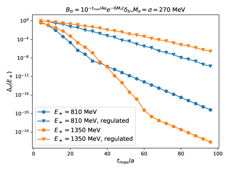
Figure 1: Relative systematic error on the kernel reconstruction $\Delta_{\sigma}(E_{\ast})$, see Eq. (2.7)

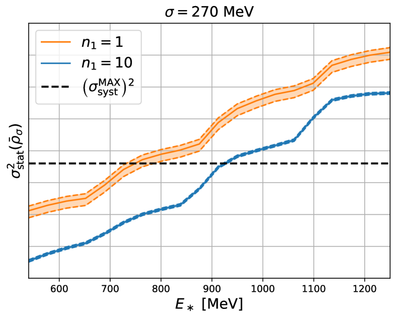
Figure 2: Statistical errors on $\bar{\rho}_{\sigma}(E_{\ast})$ at $\lambda_{\ast}:\sigma_{\mathrm{syst}}^{\text{MAX}}(\lambda_{\ast},E_{\ast})=0.02$ $\forall\,E_{\ast}$ for $n_{1}=1,10$

The extraction of smeared spectral densities from lattice correlation functions in Eq. (1.1) can involve different correlator-dependent choices of basis functions $b_{t}(E)$. In our case, $C(t)$ is the zero-momentum two-point function of two isovector vector currents and $b_{t}(E)=E^{2}\left(e^{-tE}+e^{-(T-t)E}\right)$, with $T$ the extent of the time direction along which we impose (anti-)periodic boundary conditions for bosons (fermions). We are interested in extracting smeared spectral densities

$$\rho_{\sigma}(E_{\ast})=\int_{E_{0}}^{\infty}dE\,\rho(E)\delta_{\sigma}(E,E_{\ast}),\quad\text{with }\delta_{\sigma}(E,E_{\ast})=\frac{1}{\sqrt{2\pi\sigma^{2}}}e^{-(E-E_{\ast})^{2}/2\sigma^{2}}$$ (2.2)

such that, as $\sigma\to 0$, $\delta_{\sigma}(E,E_{\ast})\to\delta(E-E_{\ast})$ and we recover $\rho_{\sigma}(E_{\ast})\to\rho(E_{\ast})$. The kernel $\delta_{\sigma}$ is approximated with the basis functions as

$$\sum_{t=t_{\mathrm{min}}}^{t_{\mathrm{max}}}b_{t}(E)g_{t}(E_{\ast})=\bar{\delta}_{\sigma}(E,E_{\ast})\approx\delta_{\sigma}(E,E_{\ast}),$$ (2.3)

where we usually consider $t_{\mathrm{min}}=a$ and require $t_{\mathrm{max}}<T/2$, so that

$$\sum_{t=t_{\mathrm{min}}}^{t_{\mathrm{max}}}C(t)g_{t}(E_{\ast})=\int_{E_{0}}^{\infty}dE\,\rho(E)\bar{\delta}_{\sigma}(E,E_{\ast})\equiv\bar{\rho}_{\sigma}(E_{\ast})\approx\rho_{\sigma}(E_{\ast})\,.$$ (2.4)

The computation of the coefficients $\{g_{t}(E_{\ast})\}_{t=t_{\mathrm{min}}}^{t_{\mathrm{max}}}$ is done by minimizing the error functional

$$\mathcal{W}[g]=\int_{E_{0}}^{\infty}dE\,\left[\delta_{\sigma}(E,E_{\ast})-\bar{\delta}_{\sigma}(E,E_{\ast})\right]^{2}+\sum_{t,r=t_{\mathrm{min}}}^{t_{\mathrm{max}}}g_{t}(E_{\ast})B_{tr}g_{r}(E_{\ast})$$ (2.5)

where the first term measures the systematic error on the kernel reconstruction and the second one acts as a regulator in the sense explained below. We obtain $g_{t}(E_{\ast})=\left[W^{-1}f(E_{\ast})\right]_{t}$, where

$$W=A+B,\quad A_{tr}=\int_{E_{0}}^{\infty}dE\,b_{t}(E)b_{r}(E),\quad f_{t}(E_{\ast})=\int_{E_{0}}^{\infty}dE\,b_{t}(E)\delta_{\sigma}(E,E_{\ast})\,.$$ (2.6)

By setting $B=0$, the coefficients are expressed in terms of $A^{-1}$, where $A$, for the choice $b_{t}(E)=e^{-tE}$, is a Cauchy matrix directly related to the Hilbert matrix, a notably ill-conditioned matrix. It is well-known, see e.g. Ref. [6], that this results in large oscillations in $g_{t}(E_{\ast})$, and statistical fluctuations on $C(t)$ then induce large statistical errors on $\bar{\rho}_{\sigma}$. This is a manifestation of the ill-posed nature of the inverse Laplace transform applied to a finite set of discrete data with statistical error, the case of Lattice QCD. In order to mitigate this problem, we may regularize the near-zero eigenvalues of $A$ by setting $B\neq 0$, adding yet another source of systematic error, besides the one due to $t_{\mathrm{max}}<\infty$. In [5, 6] it was proposed to consider $B$ to be proportional to the covariance matrix of data Cov. In principle, other types of regularizations that do not depend on data can be employed, e.g. we can consider $B=\lambda\mathbf{1}$ (Tikhonov regularization) or $B_{tr}=\lambda e^{-Mt}\delta_{tr}$, where $\lambda,aM\in[0,\infty)$, so that $B\to\lambda\mathbf{1}$ for $aM\to 0$, and $B\to 0$ for $aM\to\infty$. In Fig. 2 we show how the (relative) systematic error on the kernel reconstruction

$$\Delta_{\sigma}(E_{\ast})=\frac{\int_{E_{0}}^{\infty}dE\,\left[\delta_{\sigma}(E,E_{\ast})-\bar{\delta}_{\sigma}(E,E_{\ast})\right]^{2}}{\int_{E_{0}}^{\infty}dE\,\delta_{\sigma}(E,E_{\ast})^{2}}=1-\frac{\sum_{t,r=a}^{t_{\mathrm{max}}}f_{t}(E_{\ast})[A^{-1}]_{tr}f_{r}(E_{\ast})}{\int_{E_{0}}^{\infty}dE\,\delta_{\sigma}(E,E_{\ast})^{2}}$$ (2.7)

decreases as we increase $t_{\mathrm{max}}$ or remove the regulator $B$. On the other hand, $B$ is needed to regularize $A$, taming the statistical fluctuations on $\bar{\rho}_{\sigma}$, an effect that is evident in Fig. 3(a). The regulator parameter $\lambda$ should then be tuned in order to minimize the statistical fluctuations $\sigma_{\mathrm{stat}}$ while controlling the systematic errors $\sigma_{\mathrm{syst}}$ on $\bar{\rho}_{\sigma}$, where we define

$$\sigma_{\mathrm{stat}}^{2}(\lambda,E_{\ast})=\sum_{t,r=t_{\mathrm{min}}}^{t_{\mathrm{max}}}g_{t}(E_{\ast})\text{Cov}_{tr}g_{r}(E_{\ast}),\quad\sigma_{\mathrm{syst}}(\lambda,E_{\ast})=|\rho_{\sigma}(E_{\ast})-\bar{\rho}_{\sigma}(E_{\ast})|\,.$$ (2.8)

Since we do not have access to the true value $\rho_{\sigma}$, different estimates of $\sigma_{\mathrm{syst}}$ can be given, see e.g. in Refs. [6, 16]. Here we use the following definition

$$\sigma_{\mathrm{syst}}(\lambda,E_{\ast})\leq\rho_{max}\int_{2M_{\pi}}^{6M_{\pi}}dE\,\left|\delta_{\sigma}(E,E_{\ast})-\bar{\delta}_{\sigma}(E,E_{\ast})\right|\equiv\sigma_{\mathrm{syst}}^{\text{MAX}}(\lambda,E_{\ast})$$ (2.9)

which is an upper bound on the systematic error for $\rho_{\sigma}$ at small energies, if $\rho(E)\geq 0$ $\forall\,E$ and $\rho(E)\leq\rho_{max}\equiv\max_{E}\rho(E)$ $\forall E\in[2M_{\pi},6M_{\pi}]$; preliminary results with $\lambda$ tuned so that $\sigma_{\mathrm{stat}}(\lambda_{\ast},E_{\ast})=\sigma_{\mathrm{syst}}^{\text{MAX}}(\lambda_{\ast},E_{\ast})$ are presented in Sect. 3. A proper analysis without the restriction of the integral in Eq. (2.9) to $6M_{\pi}$ is ongoing. A different strategy that is currently being explored consists in estimating

$$\rho_{\sigma}(E_{\ast})-\bar{\rho}_{\sigma}(E_{\ast})=\int_{E_{0}}^{\infty}dE\,\left[\delta_{\sigma}(E,E_{\ast})-\bar{\delta}_{\sigma}(E,E_{\ast})\right]\rho(E)\equiv\int_{E_{0}}^{\infty}dE\,\delta_{\sigma}^{(1)}(E,E_{\ast})\rho(E)$$ (2.10)

by means of a second reconstruction with the smearing kernel $\delta_{\sigma}^{(1)}(E,E_{\ast})$.

3 Multi-level algorithm and spectral densities

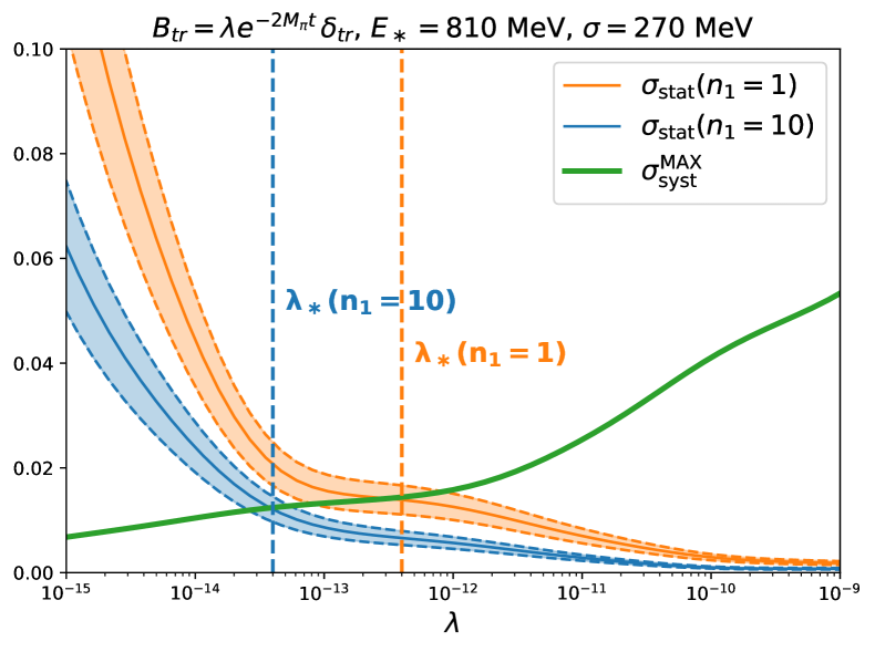
(a) Tuning of $\lambda$

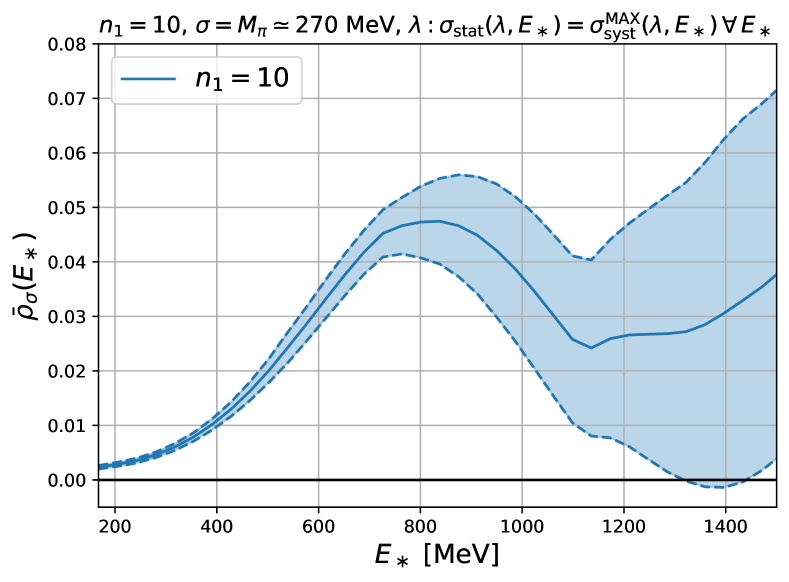
(b) $\bar{\rho}_{\sigma}$

Figure 3: Reconstruction of $\bar{\rho}_{\sigma}(E_{\ast})$ at $n_{1}=1,10$, tuning $\lambda:\sigma_{\mathrm{stat}}(\lambda_{\ast},E_{\ast})=\sigma_{\mathrm{syst}}^{\text{MAX}}(\lambda_{\ast},E_{\ast})$ $\forall\,E_{\ast}$

In this Section, we present preliminary numerical results for the extraction of smeared spectral densities from lattice correlation functions measured with the multi-level algorithm. In lattice calculations, many physically relevant observables suffer from an exponentially decreasing signal-to-noise ratio (StN) [17]. If the action and the observable dependence on the field variables can be factorized e.g. in two local domains as in [12, 13, 14, 7], we can alternate $n_{0}$ independent global (level-0) updates of the field configuration with $n_{1}$ (level-1) updates of the local regions only. Combining configurations from different local domains results in an exponential gain in the StN:

$$\frac{C(t)}{\sigma_{\mathrm{stat}}(t)}\propto n_{0}\cdot n_{1}^{2}\,e^{-(M_{\rho}-2M_{\pi})t}\,.$$ (3.11)

The factorization is straightforward for pure gauge theories [9], and tremendous theoretical and numerical progress has been recently made for theories with dynamical fermions [9, 10, 11, 12, 13, 14, 15].

The configurations were generated in Ref. [7] for $N_{\mathrm{f}}=2$ dynamical $O(a)$-improved Wilson fermions on a $96\times 48^{3}$ lattice with spacing $a=0.065$ fm and pion mass $M_{\pi}\simeq 270$ MeV, so that $M_{\pi}L\simeq 4.3$. The local, unimproved discretization of the vector current was used, with the value of the renormalization factor $Z_{V}$ at $\beta=5.3$ taken from Ref. [18].
First, we study the extraction of $\bar{\rho}_{\sigma}(E_{\ast})$ at a fixed value of $\sigma_{\mathrm{syst}}^{\text{MAX}}=0.02$ $\forall\,E_{\ast}$ by tuning $\lambda$ accordingly. In Fig. 2 we show the statistical errors for $n_{1}=1$ and $n_{1}=10$ with a Gaussian kernel of width $\sigma=M_{\pi}\simeq 270$ MeV and a regulator of the form $B_{tr}=\lambda e^{-2M_{\pi}t}\delta_{tr}$. At a number of configurations which is $n_{1}=10$ times larger, at all energies we achieve a gain in the statistical errors of $\bar{\rho}_{\sigma}(E_{\ast})$ which ranges between $25$ and $50$. The difference from the ideal $n_{1}^{2}=100$ scaling was already observed in Ref. [7] for the variance of $C(t)$ and is compatible with the presence of a residual correlation among level-1 configurations. Thus, at fixed systematic error, the multi-level scaling of the statistical error proves to be advantageous when compared to classical, one-level ($n_{1}=1$) algorithms at the energies we probe. From the same figure we note that, in order to minimize the statistical fluctuations while keeping the systematic errors under control across all energy levels, we should increase or decrease $\lambda$ at lower or higher energies respectively.
Following this last observation, in Fig. 3(a) we tune $\lambda$ so that $\sigma_{\mathrm{stat}}(\lambda_{\ast},E_{\ast})=\sigma_{\mathrm{syst}}^{\text{MAX}}(\lambda_{\ast},E_{\ast})$ for a chosen $E_{\ast}$. We note that $n_{1}=1$ data require a larger value of $\lambda$, thus increasing the overall error. By repeating this tuning for a wider energy range, from our best data-set at $n_{1}=10$ we obtain the preliminary results shown in Fig. 3(b) for the noticeably small value of the kernel width $\sigma=M_{\pi}\simeq 270$ MeV. Similarly to other studies [6, 16], we observe an increase of the statistical error with the energy, but with our multi-level data we observe the presence of a peak, which we fit with a (smeared) Breit-Wigner ansatz; our preliminary results are compatible with the presence of a resonance but further refinements are needed to overcome the present limitations of Eq. (2.9) and to assess remaining systematic effects, including e.g. the dependence on the unphysical pion mass.

4 Conclusions and outlook

The multi-level sampling strategy has proved to be effective for the reconstruction of smeared hadronic spectral densities at the energies that we probed. A detailed study of the scaling properties of the error of $\rho_{\sigma}$ and the study of other channels, such as the isovector axial and isoscalar vector channels, is deferred to future publications. Here we presented some preliminary results with a conservative estimate of the systematic error (especially at lower energies), showing promising results for $\rho_{\sigma}$ with a kernel width $\sigma=M_{\pi}$. A large effort is underway to improve the definition and understanding of the systematic uncertainties associated to the extraction of smeared spectral densities. Besides the statistical and systematic errors examined here, finite-volume [8] and discretization effects will have to be taken into account as well. Finally we remark, as described in Ref. [19], that at physical $M_{\pi}$ one can directly compare Lattice QCD results for $\bar{\rho}_{\sigma}$ with experimental hadronic spectral densities smeared with the same kernel.

5 Acknowledgements

We thank M. Dalla Brida, T. Harris and M. Pepe for data availability. This work is (partially) supported by ICSC – Centro Nazionale di Ricerca in High Performance Computing, Big Data and Quantum Computing, funded by European Union – NextGenerationEU. The research of M.B. is funded through the MUR program for young researchers “Rita Levi Montalcini”.

References

- [1] \BYT. Aoyama et. al \INPhysical Reports88720201-166;
- [2] \BYY. Amhis et. al \INThe European Physical Journal C8120213;
- [3] \BYP. Gambino, M. Jung \atqueS. Schacht \INPhysics Letters B7952019386-390;
- [4] \BYG. Backus \atqueF. Gilbert \INGeophysical Journal International161968169-205;
- [5] \BYM.T. Hansen, H.B. Meyer \atqueD. Robaina \INPhysical Review D96201711;
- [6] \BYM. Hansen, A. Lupo \atqueN. Tantalo \INPhysical Review D99201905;
- [7] \BYM. Dalla Brida, L. Giusti, T. Harris \atqueM. Pepe \INPhysics Letters B8162021136191;
- [8] \BYM. Bruno \atqueM.T. Hansen in preparation;
- [9] \BYM. Lüscher \atqueP. Weisz \INJHEP09200111;
- [10] \BYM. Della Morte \atqueL. Giusti \INComput. Phys. Comput.1802009813-818;
- [11] \BYM. Della Morte \atqueL. Giusti \INComput. Phys. Comput.1802009819-826;
- [12] \BYM. Cè, L. Giusti \atqueS. Schaefer \INPhysical Review D9320169;
- [13] \BYM. Cè, L. Giusti \atqueS. Schaefer \INPhysical Review D9520173;
- [14] \BYM. Cè, L. Giusti \atqueS. Schaefer \INEPJ Web Conf.175201811005;
- [15] \BYL. Giusti \atqueM. Saccardi \INPhysics Letters B8292022137103;
- [16] \BYJ. Bulava et al. \INJHEP072022034;
- [17] \BYG. Parisi \INJHEP071984203-211; \BYG.P. Lepage \INBoulder ASI198997-120;
- [18] \BYM. Dalla Brida, T. Korzec, S. Sint \atqueP. Vilaseca \INEur. Phys. J. C79201901;
- [19] \BYETM Collaboration, C. Alexandrou et al. \INPhys. Rev. Letters1302023241901;