Theory of correlated Chern insulators in twisted bilayer graphene
Abstract
Magic-angle twisted bilayer graphene is the best studied physical platform featuring moiré potential induced narrow bands with non-trivial topology and strong electronic correlations. Despite their significance, the Chern insulating states observed at a finite magnetic field –and extrapolating to a band filling, , at zero field– remain poorly understood. Unraveling their nature is among the most important open problems in the province of moiré materials. Here we present the first comprehensive study of interacting electrons in finite magnetic field while varying the electron density, twist angle and heterostrain. Within a panoply of correlated Chern phases emerging at a range of twist angles, we uncover a unified description for the ubiquitous sequence of states with the Chern number for and . We also find correlated Chern insulators at unconventional sequences with , as well as with fractional , and elucidate their nature.
I Introduction
The twisted bilayer graphene (TBG) has been a subject of intense theoretical and experimental investigation, in no small part due to its isolated, topologicaly non-trivial, narrow bands displaying rich correlated electron physics when partially occupied [1, 2]. As the twist angle between the two graphene layers is tuned toward the magic value of [3], TBG devices show a plethora of correlated phenomena including superconductivity, correlated insulating states and (quantized) anomalous Hall effect [4, 5, 6, 7, 8, 9, 10, 11, 12, 13, 14, 15, 16, 17, 18, 19, 20, 21, 22, 23, 24, 25, 26]. The non-trivial topology of the pair of narrow bands for a given valley and spin flavor is protected by the combined two-fold rotation symmetry about the out-of-plane axis (an emergent symmetry at low twist angle) and spinless time reversal symmetry [27, 28]. The narrow band Hilbert space can thus be decomposed into a Chern and a Chern band [27, 29, 30]. One way to reveal the non-trivial topology of the narrow bands is to break via alignment with the hexagonal boron nitride substrate (hBN) and separate the Chern bands in energy. If in addition, the valley is spontaneously polarized, thus breaking , the resulting state with one electron or hole per moiré unit cell becomes a Chern insulator [31, 32, 33, 34]. Indeed, experiments have observed anomalous Hall effect (AHE) near the filling of electrons per moiré unit cell [10, 20] in hBN aligned samples. Further studies on non-aligned samples [21, 25] have also observed AHE near 1 electron per moiré unit cell. Theoretically, such zero-field Chern insulating states (zCIs) have been proposed to be energetically competitive near magic angle, when the Coulomb interaction exceeds the narrow bandwidth, even without the hBN alignment [35, 30, 36, 33].
An external magnetic field , which preserves but breaks , has been argued to be an alternative way to reveal the band topology [11, 19, 22], as evidenced by the experimental observations of correlated Chern insulating states (CCIs) with a finite Chern number and extrapolating to a band filling at [6, 7, 8, 11, 13, 14, 15, 16, 18, 19, 21, 22, 23, 25, 26]. Specifically, the most prominent sequence of CCIs has , consistent with selective population of the aforementioned Chern bands [11, 21, 22]. These experiments also report that some CCIs are stable at extremely low , suggesting that they originate from the zCIs [11, 21].
However, CCIs are also observed in TBG devices away from the magic angle (), where the bandwidth of the narrow bands is expected to be significantly larger than at , without any observation of the correlated insulators at [9]. Such CCIs appear only above a critical , below which they transition into nearly compressible states for a fixed . Similar phenomenology has also been reported in near-magic angle devices, leading to an alternative explanation of the CCIs invoking Stoner ferromagnetism within the magnetic subbands [15, 16, 23, 7], termed Hofstadter subband ferromagnets (HSFs) [15]. As argued theoretically [37, 38, 39], realistic heterostrain can also increase the bandwidth dramatically near the magic angle, likely placing many TBG devices in the intermediate coupling regime where the zCIs may not be energetically favored.
To date, the nature of these CCIs remains poorly understood. No microscopic calculation favoring either zCI or HSF has been carried out at , nor tying them to the relevant experiments. Moreover, the interplay of the CCIs with the competing states at near the magic angle, such as the intervalley coherent states (IVCs) [40, 29], the incommensurate Kekulé spiral orders (IKSs) [38], and the striped and nematic states [30, 14, 41, 42], remains unclear.
Here we report the first comprehensive study of the interacting electrons within the TBG narrow bands directly at , and construct the phase diagram for a range of twist angles, -fields and electron densities, with and without heterostrain. Consistent with the experimental observations, we find CCIs with , , , and , see Fig. 1 and Fig. S12. Such states are found to be stablized at higher fields for twist angles as high as (highest twist angle studied in this work), and for realistic heterostrain; based on analysis of their wavefunctions, we identify them as correlated Hofstadter ferromagnets (CHFs). Similar to HSFs, they correspond to selective population of the valley and spin flavors, but of the interaction-renormalized magnetic subbands (see Fig. 2). Upon lowering we find a first order phase transition into nearly compressible states at larger twist angles, or into incompressible states with intervalley coherence closer to the magic angle, at non-zero . In the absence of heretostrain and at larger twist angles we similarly observe CHFs transitioning into nearly compressible states upon lowering (see Fig. S12). As we lower the twist angle toward , the incompressible state extends to lower and crosses over into the finite analog of the zCI, approaching maximal sublattice polarization. We refer to this state as the strong coupling Chern insulator (sCI). The , and states also cross over into sCIs upon decreasing the twist angle, but they experience a first order phase transition into IVCs at low twist angles. The details of this transition depend sensitively on the model parameters, as shown in Fig. 3 and Fig. S20. Because there is no symmetry distinction between them, the CHF smoothly crosses over into the sCI as the twist angle is decreased toward the magic angle. In the phase diagram both with and without heterostrain, in addition to these prominent CCIs, we also find Quantum Hall ferromagnetic states (QHFMs) emanating from band edges (Figs. S6, S14) and the charge neutrality point (Figs. S7, S15), CCIs with , as well as fractional that break the magnetic translation symmetry (Figs. 4, S9, S17).
II Model and method:
We perform self-consistent Hartree-Fock analysis (B-SCHF) at using the continuum Bistritzer-MacDonald (BM) Hamiltonian, with Coulomb interactions projected onto the narrow band Hilbert space. Here we briefly outline the formalism, additional details are in the Supplementary Information (SI). Starting with the (strained) BM Hamiltonian at rational magnetic flux ratios where and are coprime integers, is the magnetic flux per moiré unit cell and is the magnetic flux quantum, we solve for the Hofstadter spectra and associated eigenstates . Here and are valley and spin quantum numbers, is the magnetic subband index, and is the magnetic crystal momentum defined in the magnetic Brillouin zone with and , and are moiré reciprocal lattice vectors (see SI). Spin Zeeman splitting is also considered in this calculation. For the model parameters studied in this work, the gap to remote Hofstadter bands does not close at the magnetic fluxes of interest. We study interaction effects by projecting the screened Coulomb interaction onto the narrow band Hilbert space. The Hamiltonian is given by:
| (1) |
Here is the total area of the system, is the electron annihilation operator, is the Fourier transform of the electron density operator projected onto the narrow bands, subtracting a background charge density [43, 44, 45]. It is given by:
We consider a dual-gate screened Coulomb interaction of the form , with relative dielectric constant and screening length , where are the primitive moiré unit cell vectors (see SI). These parameters are chosen to match the overall change of chemical potential from empty to full occupation of the narrow bands in magic angle devices as extracted from the compressibility measurements as well as STM [6, 46, 47, 7, 48] (see also Fig. S2).
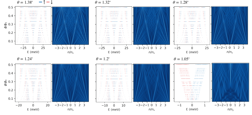
The B-SCHF calculation is carried out for a range of twist angles from to , both for unstrained model as well as for realistic uniaxial heterostrain strength of and orientation (see SI for details). The respective non-interacting Hofstadter spectra and Wannier diagrams are shown in Fig. S1 and S11.
The projected Hamiltonian at is invariant under the following set of symmetries [49, 43, 50]: , valley and spin , many-body particle-hole , magnetic translation symmetries generated by and (see SI). In the absence of heterostrain and also leave invariant. guarantees symmetry about the charge neutrality point, and therefore we present our results for the hole filling only.
III Results
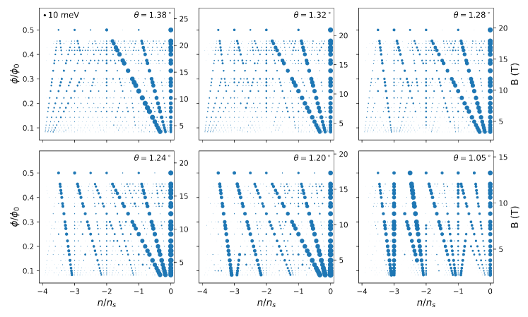
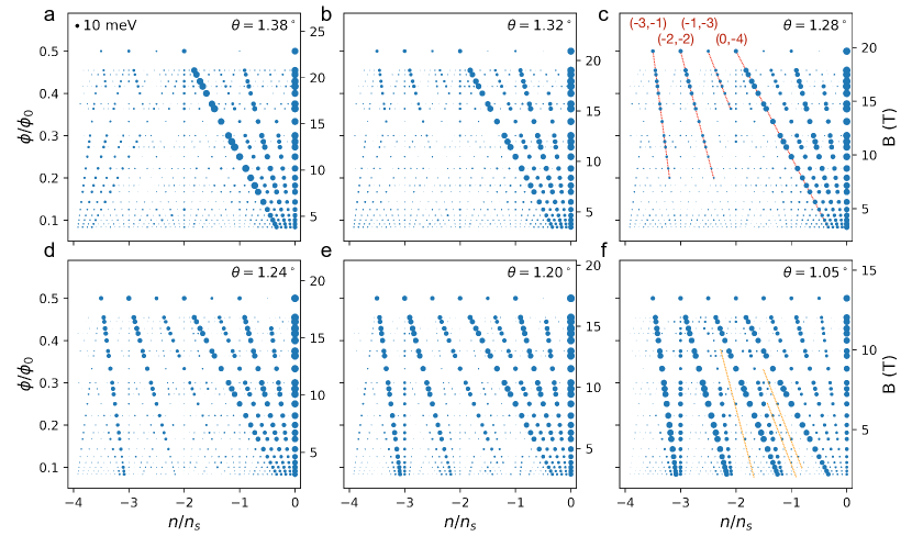
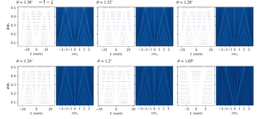
We first address the finite phase diagram for TBG subject to of heterostrain. Fig. 1 gives an overview of the calculated single particle excitation gap as a function of moiré unit cell filling () and magnetic flux ratio () for six twist angles , , , , and . The size of the gap is proportional to the radius of the solid circle. As seen, there is a rich panoply of correlated insulating states. We start by focusing on the sequence of CCIs with , which are observed for all the twist angles studied, and marked in red in Fig. 1(c). At larger twist angles, CCIs along emerge at high , and are replaced by nearly compressible states at lower via a first order phase transition. As the twist angle is lowered, they become more robust and can persist beyond the lowest flux ratio of studied in this work.
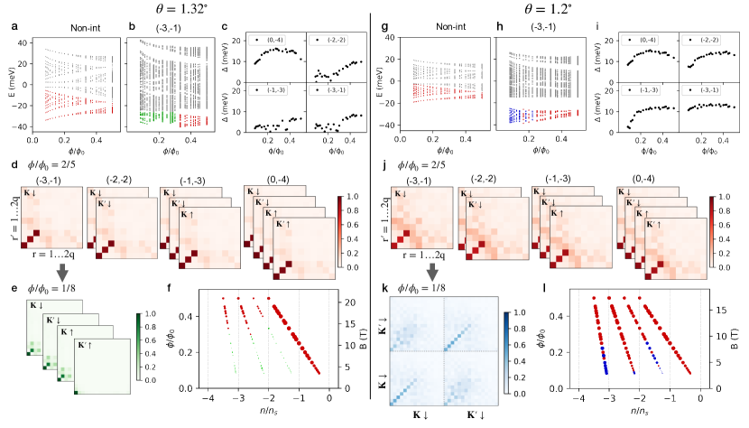
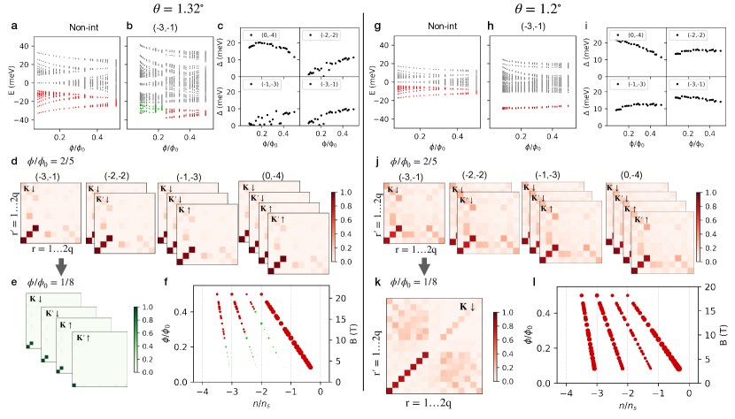
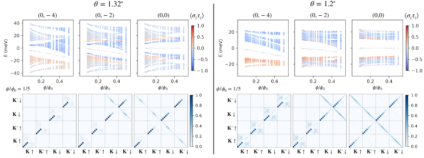
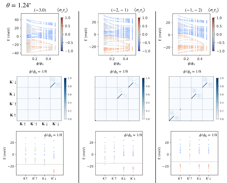
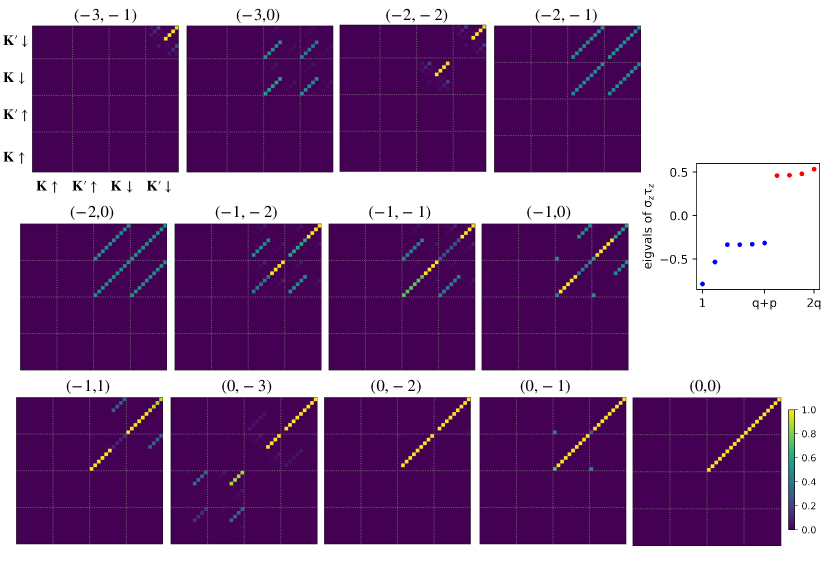
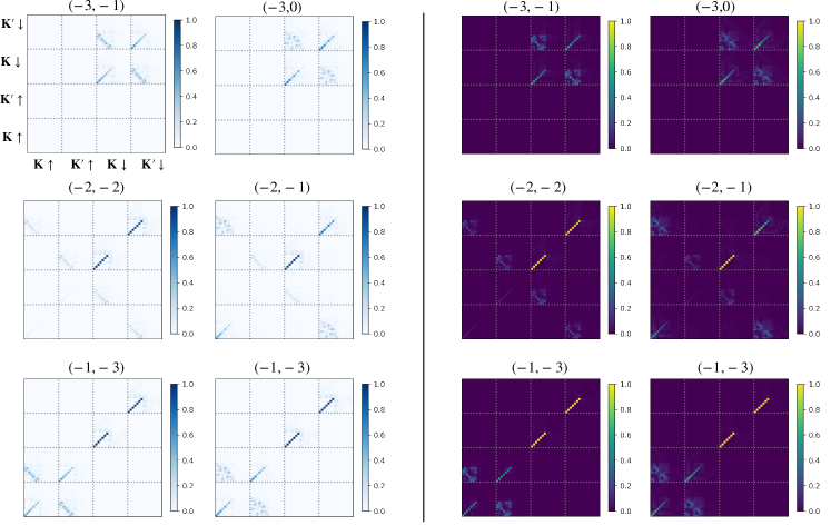
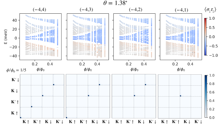
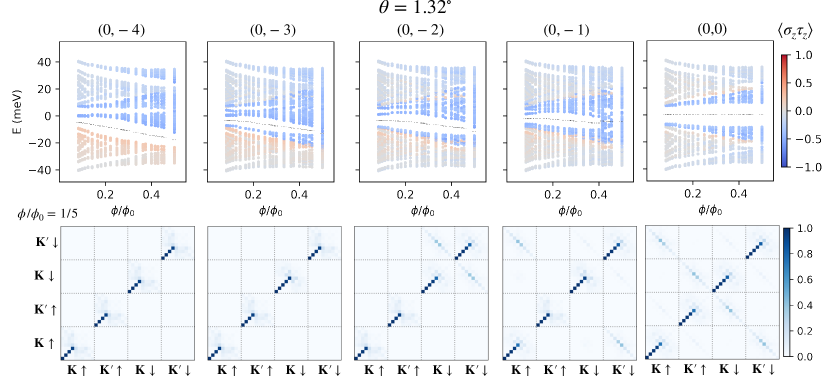
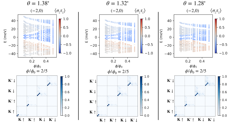
To better understand their nature, we compile detailed results for two representative twist angles [Figs. 2(a) to (f)] and [Figs. 2(g) to (l)]. Fig. 2(a) shows the non-interacting spectra of valley and for one spin component (neglecting Zeeman effect) at . The magnetic subbands marked in red denote the Chern -1 group below the charge neutrality point. The analogous group of subbands above the charge neutrality point is related to it by particle hole symmetry, and also carries total Chern number . The remaining two subbands emanate from the zeroth Landau levels (zLLs) of the energetically split Dirac points, and carry Chern number each, such that the total Chern number of all magnetic subbands is zero. Fig. 2(b) shows the single-particle spectra including Coulomb interactions along . At , the spectrum is gapped and the occupied states marked in red have a large overlap onto the states marked in red in Fig. 2(a). To quantify the overlap we make use of the Hartree-Fock density matrix, defined as ; for a state with unbroken valley and spin symmetries, it has the spin-valley diagonal form . At high , the CCI is valley and spin polarized. A representative is shown in Fig. 2(d). It is predominantly diagonal in the magnetic subband index, mostly occupying the lower magnetic subbands, i.e., the group states with total Chern -1 marked red in Fig. 2(a). At lower , the gapped spectrum (red) in Fig. 2(b) transitions into a nearly gapless spectrum (green) via a first order phase transition. These low states do not break the valley and spin symmetries, and their illustrative density matrix is shown in the Fig. 2(e). For and the density matrices of the CCIs at higher are also shown in Fig. 2(d). These CCIs are also valley and spin polarized, similarly mostly populating the lower Chern group of magnetic subbands for the specified valley and spin. are identical for all occupied flavors. As shown in Fig. 2(f), CCIs along , and display quantitative differences in the critical . In a recent transport experiment [17], the spin polarizations of the CCIs near the magic angle are identified, with and being spin polarized, and being spin unpolarized. To better explain experiments, in particular the particle-hole asymmetry, microscopic modeling beyond the Bistritzer-MacDonald Hamiltonian is required [51], which is to be studied in future works.
Although these CCIs are closely related to the HSFs discussed in Ref. [15, 7, 23], the band structure renormalization is apparent in the non-vanishing off-diagonal matrix elements of , signifying hybridization with the higher energy subbands (marked by grey in Fig. 2(a)). For this reason we refer to them as CHFs. As further demonstrated in Fig. S3, the density matrices of the CHFs assume a much simpler structure when expressed in the eigenbasis of the valley and spin symmetric Chern insulating state, which limits to an interaction-renormalized semimetal at (see Fig. S2) [38]. Finally, in Fig. 2(c) we show the evolution of the single particle gap as a function of along , , , and . Generically, the gap shows a broad plateau and non-monotonic dependence on .
At the lower twist angle of the CHFs at larger are very similar to those at higher twist angles, however with stronger hybridization into the higher energy magnetic subbands, as seen in Fig. 2(j). In contrast to , the CHFs lose via a first order phase transition to gapped states with intervalley coherence at lower , as is apparent in the non-zero matrix elements illustrated in Fig. 2(k). The intervalley coherent state may also break the magnetic translation symmetry . However, our B-SCHF calculations cannot determine a unique wavevector associated with the translation symmetry breaking, suggesting that there is a manifold of intervalley coherent states with similar energies [38]. Interestingly, such intervalley coherent states hybridize subbands from the lower half of the (renormalized) Hofstadter spectra in each valley (see Fig. S5), similar to the IKS ground states at discussed in Ref. [38].

III.1 Crossover to strong coupling regime
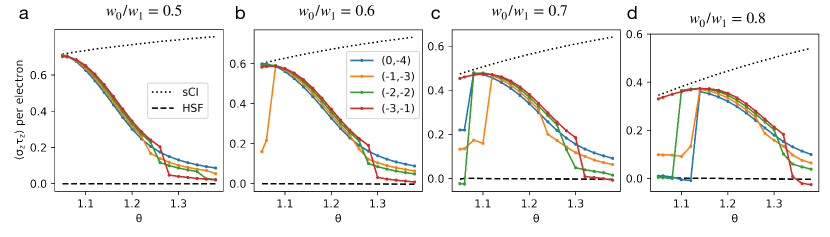
In order to clarify the connection between the CHFs and the sCIs, we first note that the sCIs saturate the expectation value of for the occupied electronic states, where and are Pauli matrices acting in the sublattice and valley subspace respectively [29, 30, 43, 45]. The solid lines in Fig. 3(a) and (b) show calculated per electron as a function of twist angle in the presence of heterostrain along , , , and , for and respectively. For comparison, the upper dashed line corresponds to the sCI limit, and the lower dashed line to the HSF limit. This measure shows that the CHFs are clearly distinct from both the HSFs and the sCIs in the presence of heterostrain. Qualitatively, the Coulomb repulsion favors an increased . The abrupt jump as angle is tuned (e.g., for in Fig. 3(b) ) marks the first order transition between the aforementioned nearly compressible state and the CHF.
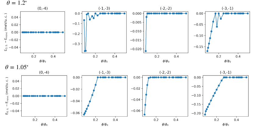
On the other hand, in the absence of heterostrain, as shown in Fig. 3(c) and (d), the CHFs smoothly crosses over into the sCIs upon lowering the twist angle. For our model parameters, there is a collapse of the at lower twist angles, when the CHFs become energetically less favorable than populating the Landau quantized excitation spectra of the IVC states [45, 40, 33, 52]. As further demonstrated in Fig. S20, this transition depends sensitively on model parameters, and can be pushed toward lower (e.g., by moving toward the chiral limit, see SI and Ref. [53]). Refs. [21, 11] report that the persist down to , and therefore argue that they correspond to the zCIs (more precisely, sCIs). Our quantitative calculations clearly demonstrate that such states can indeed be stablized at weak fields by small changes of the model parameters.
III.2 Additional CCIs
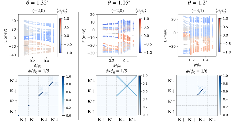
Besides the aforementioned CCIs, we also find additional correlated insulating states in the phase diagram with heterostrain (Fig. 1). The most prominent states emanate from the charge neutrality point (), and are identified as QHFMs within the zLLs of the energetically split Dirac cones [54, 55, 56] (see Figs. S7). QHFMs emanating from the band bottom () are well developed at but become progressively weaker as the angle decreases (see Figs. S6). Moreover, at higher a gapped state with is observed in Figs. 1(a-c). We identify it as a Quantum Spin Hall (QSH) insulator due to strong spin splitting near , as demonstrated in the non-interacting Hofstadter spectra in Fig. S1 and the density matrices in Fig. S8.
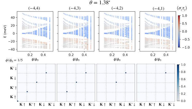
Closer to the magic angle, we also find unusual sequences with . These states have the same as the sequence discussed previously, but with a Chern number that is higher by . They all have intervalley coherence, with structure of the density matrices resembling that of an IKS ground state. However, careful analysis shows that they do not correspond to populating the Landau quantized excitation spectra of the CCIs along . Rather, they are distinct intervalley coherent states with a regorganization of the intervalley coherence between the magnetic subbands (see Fig. S5).
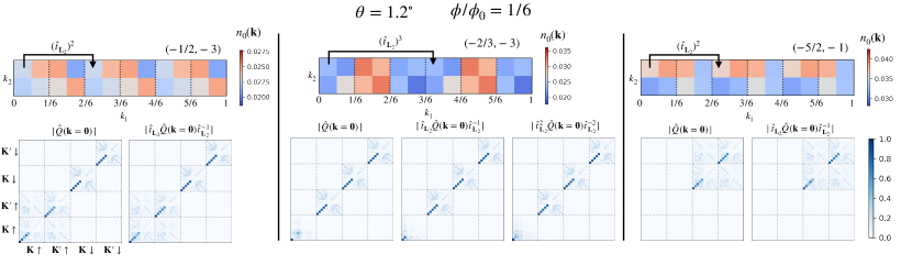
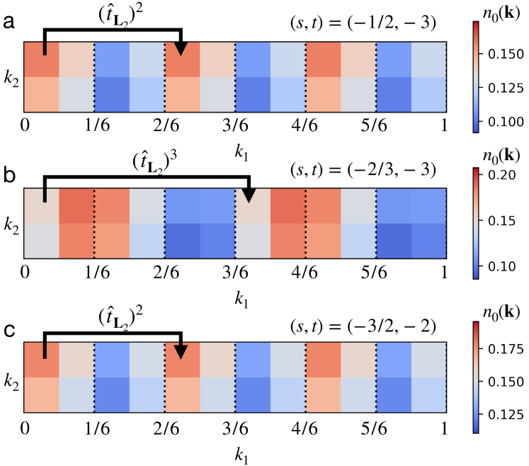
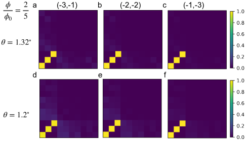
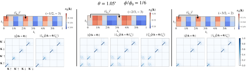
At , we also find CCIs with fractional along , , and , see Fig. 1(f). These states break magnetic translation symmetry. We identify them as striped states with period along the direction, such that the density matrix is invariant under . Their respective density matrices are shown in Fig. S9. We use the electron occupation number of the lower zLL (see Fig. 2(a) and (i) for example) in valley and for spin to illustrate the striped states. We define it as , and show its momentum dependence in the magnetic Brillouin zone at for , , and in Figs. 4 (a), (b) and (c) respectively. At and , the fractional part of corresponds to half-filling of a valley and spin flavor, and we identify the period of the striped state as . At , the fractional part of corresponds to two thirds filling of a flavor, and we identify the stripe period as .
IV Conclusion
In summary, by performing a comprehensive self-consistent Hartree-Fock study of the continuum Bistritzer-MacDonald model in finite magnetic fields, we unravel the nature of the prominent correlated Chern insulators observed in a wide range of TBG experiments. For realistic heterostrain, these CCIs are stablized at higher magnetic fields, and correspond to valley and spin polarizations of the interaction-renormalized magnetic subbands (CHFs). Upon lowering magnetic field, the CHFs become energetically less favored, losing to nearly compressible states at larger twist angles and other gapped states with intervalley coherence at smaller twist angles. In absence of heterostrain and at higher magnetic fields, the CHF crosses over to the strong coupling Chern insulating states (sCIs) as the twist angle decreases. At lower fields, competing states with intervalley coherence become more energetically favored, and the transition is marked by a collapse of the averaged sublattice polarization per occupied single-electron state.
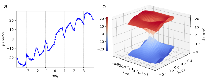
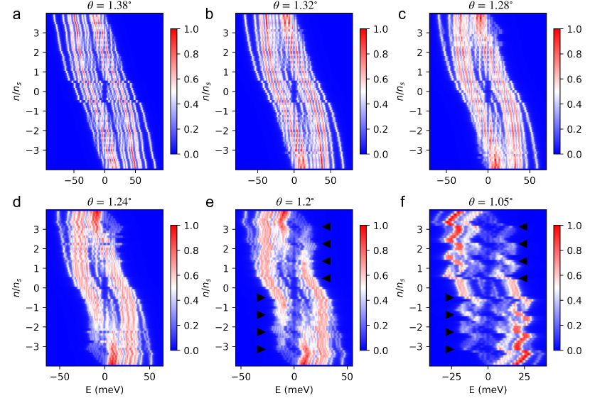
Our calculations also predict additional gapped correlated insulating states beyond the sequence, notably the striped states at fractional . Given that our calculations have direct access to the interaction renormalized single-electron excitation spectra at a given filling and magnetic field (see Fig. S10), comparisons with experiments such as STM can be made to facilitate the characterization of the panoply of correlated insulating states.
V Acknowledgements
X.W. and O. V. acknowledge invaluable discussions with B. Andrei Bernevig, C. Lewandowski, J. Finney, M.-H. He and J. Kang. X.W. acknowledges financial support from the Gordon and Betty Moore Foundation’s EPiQS Initiative Grant GBMF11070, National High Magnetic Field Laboratory through NSF Grant No. DMR-1157490 and the State of Florida. O.V. was supported by NSF Grant No. DMR-1916958 and is partially funded by the Gordon and Betty Moore Foundation’s EPiQS Initiative Grant GBMF11070. Most of the computing for this project was performed on the HPC at the Research Computing Center at the Florida State University (FSU).
References
- Andrei and MacDonald [2020] E. Y. Andrei and A. H. MacDonald, Graphene bilayers with a twist, Nature Materials 19, 1265 (2020).
- Balents et al. [2020] L. Balents, C. R. Dean, D. K. Efetov, and A. F. Young, Superconductivity and strong correlations in moiré flat bands, Nature Physics 16, 725 (2020).
- Bistritzer and MacDonald [2011] R. Bistritzer and A. H. MacDonald, Moiré bands in twisted double-layer graphene, Proceedings of the National Academy of Sciences 108, 12233 (2011).
- Cao et al. [2018a] Y. Cao, V. Fatemi, A. Demir, S. Fang, S. L. Tomarken, J. Y. Luo, J. D. Sanchez-Yamagishi, K. Watanabe, T. Taniguchi, E. Kaxiras, R. C. Ashoori, and P. Jarillo-Herrero, Correlated insulator behaviour at half-filling in magic-angle graphene superlattices, Nature 556, 80 (2018a).
- Cao et al. [2018b] Y. Cao, V. Fatemi, S. Fang, K. Watanabe, T. Taniguchi, E. Kaxiras, and P. Jarillo-Herrero, Unconventional superconductivity in magic-angle graphene superlattices, Nature 556, 43 (2018b).
- Tomarken et al. [2019] S. L. Tomarken, Y. Cao, A. Demir, K. Watanabe, T. Taniguchi, P. Jarillo-Herrero, and R. C. Ashoori, Electronic compressibility of magic-angle graphene superlattices, Phys. Rev. Lett. 123, 046601 (2019).
- Park et al. [2021] J. M. Park, Y. Cao, K. Watanabe, T. Taniguchi, and P. Jarillo-Herrero, Flavour hund’s coupling, chern gaps and charge diffusivity in moiré graphene, Nature 592, 43 (2021).
- Xie et al. [2019] Y. Xie, B. Lian, B. Jäck, X. Liu, C.-L. Chiu, K. Watanabe, T. Taniguchi, B. A. Bernevig, and A. Yazdani, Spectroscopic signatures of many-body correlations in magic-angle twisted bilayer graphene, Nature 572, 101 (2019).
- Yankowitz et al. [2019] M. Yankowitz, S. Chen, H. Polshyn, Y. Zhang, K. Watanabe, T. Taniguchi, D. Graf, A. F. Young, and C. R. Dean, Tuning superconductivity in twisted bilayer graphene, Science 363, 1059 (2019).
- Sharpe et al. [2019] A. L. Sharpe, E. J. Fox, A. W. Barnard, J. Finney, K. Watanabe, T. Taniguchi, M. A. Kastner, and D. Goldhaber-Gordon, Emergent ferromagnetism near three-quarters filling in twisted bilayer graphene, Science 365, 605 (2019).
- Nuckolls et al. [2020] K. P. Nuckolls, M. Oh, D. Wong, B. Lian, K. Watanabe, T. Taniguchi, B. A. Bernevig, and A. Yazdani, Strongly correlated chern insulators in magic-angle twisted bilayer graphene, Nature 588, 610 (2020).
- Nuckolls et al. [2023] K. P. Nuckolls, R. L. Lee, M. Oh, D. Wong, T. Soejima, J. P. Hong, D. Călugăru, J. Herzog-Arbeitman, B. A. Bernevig, K. Watanabe, T. Taniguchi, N. Regnault, M. P. Zaletel, and A. Yazdani, Quantum textures of the many-body wavefunctions in magic-angle graphene, Nature 620, 525 (2023).
- Pierce et al. [2021] A. T. Pierce, Y. Xie, J. M. Park, E. Khalaf, S. H. Lee, Y. Cao, D. E. Parker, P. R. Forrester, S. Chen, K. Watanabe, T. Taniguchi, A. Vishwanath, P. Jarillo-Herrero, and A. Yacoby, Unconventional sequence of correlated chern insulators in magic-angle twisted bilayer graphene, Nature Physics 17, 1210 (2021).
- Xie et al. [2021] Y. Xie, A. T. Pierce, J. M. Park, D. E. Parker, E. Khalaf, P. Ledwith, Y. Cao, S. H. Lee, S. Chen, P. R. Forrester, K. Watanabe, T. Taniguchi, A. Vishwanath, P. Jarillo-Herrero, and A. Yacoby, Fractional chern insulators in magic-angle twisted bilayer graphene, Nature 600, 439 (2021).
- Saito et al. [2021a] Y. Saito, J. Ge, L. Rademaker, K. Watanabe, T. Taniguchi, D. A. Abanin, and A. F. Young, Hofstadter subband ferromagnetism and symmetry-broken chern insulators in twisted bilayer graphene, Nature Physics 17, 478 (2021a).
- Yu et al. [2022] J. Yu, B. A. Foutty, Z. Han, M. E. Barber, Y. Schattner, K. Watanabe, T. Taniguchi, P. Phillips, Z.-X. Shen, S. A. Kivelson, and B. E. Feldman, Correlated hofstadter spectrum and flavour phase diagram in magic-angle twisted bilayer graphene, Nature Physics 18, 825 (2022).
- Hoke et al. [2023] J. C. Hoke, Y. Li, J. May-Mann, K. Watanabe, T. Taniguchi, B. Bradlyn, T. L. Hughes, and B. E. Feldman, Uncovering the spin ordering in magic-angle graphene via edge state equilibration (2023), arXiv:2309.06583 .
- Lu et al. [2019] X. Lu, P. Stepanov, W. Yang, M. Xie, M. A. Aamir, I. Das, C. Urgell, K. Watanabe, T. Taniguchi, G. Zhang, A. Bachtold, A. H. MacDonald, and D. K. Efetov, Superconductors, orbital magnets and correlated states in magic-angle bilayer graphene, Nature 574, 653 (2019).
- Das et al. [2021] I. Das, X. Lu, J. Herzog-Arbeitman, Z.-D. Song, K. Watanabe, T. Taniguchi, B. A. Bernevig, and D. K. Efetov, Symmetry-broken chern insulators and rashba-like landau-level crossings in magic-angle bilayer graphene, Nature Physics 17, 710 (2021).
- Serlin et al. [2020] M. Serlin, C. L. Tschirhart, H. Polshyn, Y. Zhang, J. Zhu, K. Watanabe, T. Taniguchi, L. Balents, and A. F. Young, Intrinsic quantized anomalous hall effect in a moiré heterostructure, Science 367, 900 (2020).
- Stepanov et al. [2021] P. Stepanov, M. Xie, T. Taniguchi, K. Watanabe, X. Lu, A. H. MacDonald, B. A. Bernevig, and D. K. Efetov, Competing zero-field chern insulators in superconducting twisted bilayer graphene, Phys. Rev. Lett. 127, 197701 (2021).
- Wu et al. [2021] S. Wu, Z. Zhang, K. Watanabe, T. Taniguchi, and E. Y. Andrei, Chern insulators, van hove singularities and topological flat bands in magic-angle twisted bilayer graphene, Nature Materials 20, 488 (2021).
- Choi et al. [2021a] Y. Choi, H. Kim, Y. Peng, A. Thomson, C. Lewandowski, R. Polski, Y. Zhang, H. S. Arora, K. Watanabe, T. Taniguchi, J. Alicea, and S. Nadj-Perge, Correlation-driven topological phases in magic-angle twisted bilayer graphene, Nature 589, 536 (2021a).
- Choi et al. [2021b] Y. Choi, H. Kim, C. Lewandowski, Y. Peng, A. Thomson, R. Polski, Y. Zhang, K. Watanabe, T. Taniguchi, J. Alicea, and S. Nadj-Perge, Interaction-driven band flattening and correlated phases in twisted bilayer graphene, Nature Physics 17, 1375 (2021b).
- Grover et al. [2022] S. Grover, M. Bocarsly, A. Uri, P. Stepanov, G. Di Battista, I. Roy, J. Xiao, A. Y. Meltzer, Y. Myasoedov, K. Pareek, K. Watanabe, T. Taniguchi, B. Yan, A. Stern, E. Berg, D. K. Efetov, and E. Zeldov, Chern mosaic and berry-curvature magnetism in magic-angle graphene, Nature Physics 18, 885 (2022).
- Uri et al. [2020] A. Uri, S. Grover, Y. Cao, J. A. Crosse, K. Bagani, D. Rodan-Legrain, Y. Myasoedov, K. Watanabe, T. Taniguchi, P. Moon, M. Koshino, P. Jarillo-Herrero, and E. Zeldov, Mapping the twist-angle disorder and landau levels in magic-angle graphene, Nature 581, 47 (2020).
- Po et al. [2019] H. C. Po, L. Zou, T. Senthil, and A. Vishwanath, Faithful tight-binding models and fragile topology of magic-angle bilayer graphene, Phys. Rev. B 99, 195455 (2019).
- Song et al. [2019] Z. Song, Z. Wang, W. Shi, G. Li, C. Fang, and B. A. Bernevig, All magic angles in twisted bilayer graphene are topological, Phys. Rev. Lett. 123, 036401 (2019).
- Bultinck et al. [2020a] N. Bultinck, E. Khalaf, S. Liu, S. Chatterjee, A. Vishwanath, and M. P. Zaletel, Ground state and hidden symmetry of magic-angle graphene at even integer filling, Phys. Rev. X 10, 031034 (2020a).
- Kang and Vafek [2020] J. Kang and O. Vafek, Non-abelian dirac node braiding and near-degeneracy of correlated phases at odd integer filling in magic-angle twisted bilayer graphene, Phys. Rev. B 102, 035161 (2020).
- Zhang et al. [2019] Y.-H. Zhang, D. Mao, and T. Senthil, Twisted bilayer graphene aligned with hexagonal boron nitride: Anomalous hall effect and a lattice model, Phys. Rev. Res. 1, 033126 (2019).
- Bultinck et al. [2020b] N. Bultinck, S. Chatterjee, and M. P. Zaletel, Mechanism for anomalous hall ferromagnetism in twisted bilayer graphene, Phys. Rev. Lett. 124, 166601 (2020b).
- Lian et al. [2021] B. Lian, Z.-D. Song, N. Regnault, D. K. Efetov, A. Yazdani, and B. A. Bernevig, Twisted bilayer graphene. iv. exact insulator ground states and phase diagram, Phys. Rev. B 103, 205414 (2021).
- Liu and Dai [2021] J. Liu and X. Dai, Theories for the correlated insulating states and quantum anomalous hall effect phenomena in twisted bilayer graphene, Phys. Rev. B 103, 035427 (2021).
- Xie and MacDonald [2020] M. Xie and A. H. MacDonald, Nature of the correlated insulator states in twisted bilayer graphene, Phys. Rev. Lett. 124, 097601 (2020).
- Soejima et al. [2020] T. Soejima, D. E. Parker, N. Bultinck, J. Hauschild, and M. P. Zaletel, Efficient simulation of moiré materials using the density matrix renormalization group, Phys. Rev. B 102, 205111 (2020).
- Bi et al. [2019] Z. Bi, N. F. Q. Yuan, and L. Fu, Designing flat bands by strain, Phys. Rev. B 100, 035448 (2019).
- Kwan et al. [2021] Y. H. Kwan, G. Wagner, T. Soejima, M. P. Zaletel, S. H. Simon, S. A. Parameswaran, and N. Bultinck, Kekulé spiral order at all nonzero integer fillings in twisted bilayer graphene, Phys. Rev. X 11, 041063 (2021).
- Wang et al. [2023] X. Wang, J. Finney, A. L. Sharpe, L. K. Rodenbach, C. L. Hsueh, K. Watanabe, T. Taniguchi, M. A. Kastner, O. Vafek, and D. Goldhaber-Gordon, Unusual magnetotransport in twisted bilayer graphene from strain-induced open fermi surfaces, Proceedings of the National Academy of Sciences 120, e2307151120 (2023).
- Po et al. [2018] H. C. Po, L. Zou, A. Vishwanath, and T. Senthil, Origin of mott insulating behavior and superconductivity in twisted bilayer graphene, Phys. Rev. X 8, 031089 (2018).
- Liu et al. [2021] S. Liu, E. Khalaf, J. Y. Lee, and A. Vishwanath, Nematic topological semimetal and insulator in magic-angle bilayer graphene at charge neutrality, Phys. Rev. Res. 3, 013033 (2021).
- Xie et al. [2023] F. Xie, J. Kang, B. A. Bernevig, O. Vafek, and N. Regnault, Phase diagram of twisted bilayer graphene at filling factor , Phys. Rev. B 107, 075156 (2023).
- Bernevig et al. [2021] B. A. Bernevig, Z.-D. Song, N. Regnault, and B. Lian, Twisted bilayer graphene. iii. interacting hamiltonian and exact symmetries, Phys. Rev. B 103, 205413 (2021).
- Vafek and Kang [2020] O. Vafek and J. Kang, Renormalization group study of hidden symmetry in twisted bilayer graphene with coulomb interactions, Phys. Rev. Lett. 125, 257602 (2020).
- Wang and Vafek [2022] X. Wang and O. Vafek, Narrow bands in magnetic field and strong-coupling hofstadter spectra, Phys. Rev. B 106, L121111 (2022).
- Zondiner et al. [2020] U. Zondiner, A. Rozen, D. Rodan-Legrain, Y. Cao, R. Queiroz, T. Taniguchi, K. Watanabe, Y. Oreg, F. von Oppen, A. Stern, E. Berg, P. Jarillo-Herrero, and S. Ilani, Cascade of phase transitions and dirac revivals in magic-angle graphene, Nature 582, 203 (2020).
- Wong et al. [2020] D. Wong, K. P. Nuckolls, M. Oh, B. Lian, Y. Xie, S. Jeon, K. Watanabe, T. Taniguchi, B. A. Bernevig, and A. Yazdani, Cascade of electronic transitions in magic-angle twisted bilayer graphene, Nature 582, 198 (2020).
- Saito et al. [2021b] Y. Saito, F. Yang, J. Ge, X. Liu, T. Taniguchi, K. Watanabe, J. I. A. Li, E. Berg, and A. F. Young, Isospin pomeranchuk effect in twisted bilayer graphene, Nature 592, 220 (2021b).
- Hejazi et al. [2019] K. Hejazi, C. Liu, H. Shapourian, X. Chen, and L. Balents, Multiple topological transitions in twisted bilayer graphene near the first magic angle, Phys. Rev. B 99, 035111 (2019).
- Herzog-Arbeitman et al. [2022] J. Herzog-Arbeitman, A. Chew, D. K. Efetov, and B. A. Bernevig, Reentrant correlated insulators in twisted bilayer graphene at 25 t ( flux), Phys. Rev. Lett. 129, 076401 (2022).
- Kang and Vafek [2023] J. Kang and O. Vafek, Pseudomagnetic fields, particle-hole asymmetry, and microscopic effective continuum hamiltonians of twisted bilayer graphene, Phys. Rev. B 107, 075408 (2023).
- Singh et al. [2023] K. Singh, A. Chew, J. Herzog-Arbeitman, B. A. Bernevig, and O. Vafek, Topological heavy fermions in magnetic field (2023), arXiv:2305.08171 .
- Tarnopolsky et al. [2019] G. Tarnopolsky, A. J. Kruchkov, and A. Vishwanath, Origin of magic angles in twisted bilayer graphene, Phys. Rev. Lett. 122, 106405 (2019).
- Nomura and MacDonald [2006] K. Nomura and A. H. MacDonald, Quantum hall ferromagnetism in graphene, Phys. Rev. Lett. 96, 256602 (2006).
- Kharitonov [2012] M. Kharitonov, Phase diagram for the quantum hall state in monolayer graphene, Phys. Rev. B 85, 155439 (2012).
- Young et al. [2012] A. F. Young, C. R. Dean, L. Wang, H. Ren, P. Cadden-Zimansky, K. Watanabe, T. Taniguchi, J. Hone, K. L. Shepard, and P. Kim, Spin and valley quantum hall ferromagnetism in graphene, Nature Physics 8, 550 (2012).
Supplemental Material for “Theory of correlated Chern insulators in twisted bilayer graphene”
I TBG with heterostrain at zero magnetic field
We consider the limit of small twist angle and small deformations of moiré superlattice due to uniaxial heterostrain, such that the moiré reciprocal lattice vectors are given by: [37], where are reciprocal lattice vectors of the untwisted and undeformed monolayer graphene, and
| (S1) |
where
| (S2) |
Here parameterize the uniaxial heterostrain strength and orientation, is the two-dimensional rotation matrix, and is the Poisson ratio. The moiré lattice vectors are uniquely defined through the relation . Specifically,
| (S3) |
We consider the strained Bistritzer-MacDonald (BM) Hamiltonian discussed in our recent work [39], with the continuum Hamiltonian given as:
| (S4) |
where labels valleys of monolayer graphene, labels the top (bottom) of the two graphene layers. The interlayer Hamiltonian is given by:
| (S5) |
where is a spinor in the sublattice basis for a given valley and layer. We have suppressed the spin index for simplicity. are the three nearest neighbor bonds of the reciprocal honeycomb lattice, and
| (S6) |
Here are Pauli matrices acting on sublattice degrees of freedom. and are intra-sublattice and inter-sublattice tunneling strengths between the two layers. The “chiral limit” discussed in Ref. [53] corresponds to .
The intra-layer Hamiltonian is given by:
| (S7) |
where the first term is the deformation potential that couples to the electron density. is the pseudovector potential that comes from changes in the inter-sublattice hopping due to deformations, and changes sign between graphene valleys. It is given as .
We use and . We further fix , and in our calculations, and also set constants in the remainder of this document. Other values of are also used and discussed in the manuscript as a way to stablize the strong-coupling Chern insulating states.
II TBG in magnetic field
II.1 Landau level wavefunctions of monolayer graphene
We begin with a brief discussion of the Landau level (LL) eigenstates of the Dirac Hamiltonian of monolayer graphene. In a finite magnetic field , the Dirac Hamiltonian in valleys and are given by (here for negative charged electrons, the minimal coupling is where is positive):
| (S8) | ||||
| (S9) |
Here is the layer index, is the position of the Dirac cone in the reciprocal space.
We choose the Landau gauge such that the vector potential , where the global coordinate system is defined such that is along the direction. When TBG is subject to heterstrain, this amounts to a small angle rotation of the global coordinate system with respect to the case in absence of heterostrain. The eigenstates of the Dirac Hamiltonian are solved by going to the harmonic oscillator basis: , and , where is the magnetic length.
In valley , the particle-hole symmetric LL eigenstates are given as:
| (S10) |
where is the energy of the Dirac Hamiltonian, labeled by , and corresponds to positive and negative energy solutions. We have defined . In addition, there is an anomalous zero energy state given by
| (S11) |
which lives on the B sublattice. is the eigenfunction of , and is given to be:
| (S12) |
where is the Hermite polynomial. The shift in the position for a given wavevector is given by:
| (S13) |
In valley , the Landau level wavefunctions are solved in a similar manner, and the LL eigenbasis is given by:
| (S14) |
with eigenenergy , and eigenstate for the zeroth LL:
| (S15) |
For notational convenience we define a ket state such that:
| (S16) |
The ket state has the following real space properties:
| (S17) |
where the definitions of are inferred from Eqs. (S10), (S11), (S14) and (S15).
II.2 Magnetic translation group eigenstates
At rational magnetic flux ratios where is the magnetic flux quantum, and are coprime integers, the strained BM Hamiltonian is invariant under magnetic translations, and , such that:
| (S18) |
Here . As a result, the eigenstates of the strained Bistritzer-MacDonald Hamiltonian are simultaneous eigenstates of the magnetic translation group (MTG). The MTG basis states can be generated from the LL basis states discussed in the previous section:
| (S19) |
where is a normalization factor, and . It is straightforward to check that:
| (S20) | ||||
| (S21) | ||||
| (S22) | ||||
| (S23) |
Therefore, the MTG eigenstates defined in form a complete and orthornomal basis set in a finite magnetic field. This is referred to as the magnetic Brillouin zone. In order to find the eigenstates of the narrow bands for strained BM Hamiltonian in , we also need to compute the matrix elements of the interlayer tunneling terms in the above MTG basis states. From now on we work with rational flux ratio , where and are coprime.
II.3 Matrix elements for a generic operator
We first work out the matrix elements for a generic operator in the MTG eigenstates, , where is a space-independent matrix in the layer, sublattice, and valley basis. For example, the Fourier transform of the electron density operator, , has , where is the identity matrix. We denote and . We therefore have:
| (S24) |
The notation represents modulo , with . We have defined:
| (S25) |
We proceed to work out the 1D integration by noting that:
| (S26) |
and as a result:
| (S27) |
where can be expressed in terms of associated Laguerre polynomials [45], and:
| (S28) |
Next we consider the implications of the function constraints. Firstly we have:
| (S29) |
Secondly we have:
| (S30) |
This shows that above matrix elements are non-vanishing only if:
| (S31) |
Finally, we have the following expression for the matrix elements:
with .
II.4 Matrix elements of strained BM Hamiltonian
II.4.1 Interlayer terms
The interlayer terms are a special case of the generic discussed in the previous section. For bottom to top layer tunneling we have (see Eq. (S24)):
| (S32) |
where . For notational convenience we have also defined where are integers (with implicit dependence on ). Plugging these into the -function constraints we have:
| (S33) |
We can split the momentum into strips of , by redefining:
| (S34) |
It is clear then that are good quantum numbers under moire periodic potential, and that:
| (S35) |
II.4.2 Narrow band eigenstates
From above analysis, it is clear that the narrow band eigenstates in the Landau gauge are labeled by , and an additional quantum numbers per valley and spin. Generally we can denote them as:
| (S36) |
II.4.3 Degeneracy of magnetic subbands generated by
The non-interacting Hamiltonian in valley acting on the narrow band eigenstates is:
| (S37) |
We apply the magnetic translation to these energy eigenstates. Note that they are eigenstates of and ; the reason why is applied times is due to non-commuting nature of magnetic translation operators and . We see that:
| (S38) |
Furthermore since , we have:
| (S39) |
namely that is an energy eigenstate at .
This means that the tower of states are periodic with respect to , and that all the distinct energy solutions can be found in the domain of . Furthermore, the translation gives us one way of gauge fixing between values in different strips of . Specifically, we can define:
| (S40) |
as the gauge-fixed eigenstate wavefunction at . This amounts to the following definition:
| (S41) |
II.5 Matrix elements of with respect to narrow band eigenstates
This can be computed as follows:
| (S42) |
Note that here the -constraint depends on , and matrix elements are only non-vanishing for:
| (S43) |
Computing above bruteforce is costly. However we could make use of to reduce the amount of calculations by a factor of . This is seen by noting that:
| (S44) |
In the last step we made use of the constraint . Therefore, rather than calculating blocks of matrices corresponding to differences in , we only need to compute blocks, and generate all remaining ones by multiplying a global phase factor.
III Self-consistent Hartree-Fock method in finite magnetic field
We proceed to discuss the Hartree-Fock procedure in a finite magnetic field (B-SCHF). We consider the strained BM Hamiltonian in the presence of screened Coulomb interactions, and project it onto the finite field Hilbert space. The Hamiltonian is given by:
| (S45) |
where is the area of the system, is the Hofstadter spectra including spin Zeeman splitting, and is the Fourier transform of the screened Coulomb interaction. The projected density operator is given by:
| (S46) |
where . We emphasize again that the matrix elements are non-zero only for wavevectors satisfying:
| (S47) |
Here on we introduce the matrix notation for the structure factor:
| (S48) |
where we use to label spin. Pay attention that in prior contexts we have used to denote an integer.
As a result, the Coulomb piece of the Hamiltonian can be written as:
| (S49) |
where is the moiré reciprocal lattice vector. We note first on the constraint of the -functions on the allowed values of momentum. Specifically we have:
| (S50) |
Since and , the following constraint applies:
| (S51) |
III.1 Product state and one-particle density matrix
At a given filling, we consider a ground state to be a product state, given by partial fillings of the narrow band states . This is equivalent to defining a one-particle density matrix:
| (S52) |
Note that takes to , and as a result, a difference of the density matrix at and allows us to probe magnetic translation symmetry breaking of .
III.2 Hartree Fock Hamiltonian
The Hartree-Fock Hamiltonian is given as:
| (S53) |
Our B-SCHF results are obtained by minimizing Eq. S53 with respect to product state . In practice, we achieve minimization by running both random initializations for the density matrix as well as for educated guesses, such as a strong coupling Chern insulating state, flavor polarized state, intervalley coherent state, etc. Typically, the phase diagram obtained in Fig. 1 of the main text is a collection of up to 10 initializations schemes of the density matrix.
For each magnetic flux ratio , we study momentum space mesh consisting of points along direction in the range of , and points along direction in the range of , where is chosen as the maximum integer such that . Our calculations presented in the main text correspond to 23 magnetic flux ratios between and , where we take and .
IV Extended Figures
IV.1 Extended results in the presence of heterostrain
Here we present B-SCHF results obtained for various twist angles in the presence of heterostrain.
IV.2 Extended results in the absence of heterostrain
Here we present B-SCHF results obtained for various twist angles in the absence of heterostrain.