High frequency non-gyrokinetic turbulence at tokamak edge parameters

Abstract

First of a kind 6D-Vlasov computer simulations of high frequency ion Bernstein wave turbulence for parameters relevant to the tokamak edge show transport comparable to sub-Larmor-frequency gyrokinetic turbulence. The customary restriction of magnetized plasma turbulence studies to the gyrokinetic approximation may not be based on physics but only a practical constraint due to computational cost.

Five-dimensional gyrokinetic turbulence simulations have become the gold standard for theoretical transport studies in the core of magnetic confinement systems. Yet, their descriptive power still falls short of the tokamak edge-plasma and particularly the high confinement mode (H-mode) transition, likely due to the presence of high gradients ($\rho_{i}/L_{n}=O(1)$) and elevated fluctuation levels ($\delta n/n=O(1)$). On the other hand, the axioms of gyrokinetics, that the distribution function is nearly constant on a Larmor circle and the turbulence time scales long compared to the Larmor period, are ultimately just assumptions. Time and again, confined plasma has proven to evade preconceptions, such as with the unexpected finding of the importance of “hyperfine turbulence” [1] on the extremely small electron Larmor radius scale. Nevertheless, owing to the many extremely disparate time scales for strongly magnetized plasmas (e.g. for transport, gyration, Alfven-waves), there have been only steps in the direction of full 6D simulations, consisting of only two space dimensions [2] and/or linear verification with standard gyro-kinetic ion temperature gradient (ITG) modes [3], or the study of waves [4] in a gyrokinetic background. (The situation is very different from astrophysics or inertial fusion, where 6D simulations are common place.)

Using the novel 6D turbulence code BSL6D, which is particularly efficient in simulating ion gyrations [5], we demonstrate that indeed genuinely non-gyrokinetic instabilities and turbulence have to be taken into account for high gradients such as those typical for a tokamak edge.

The target of our 6D simulations is the ion kinetic equation in dimensionless ($\rho_{i}=v_{\text{th}}=n=T=1$) variables

$$\partial_{t}f+\bm{v}\cdot\nabla f+(-\nabla\phi+\bm{v}\times\bm{B})\cdot\nabla_{\bm{v}}f=0$$ (1)

where for simplicity we restrict ourselves to electrostatic perturbations in “slab geometry”, i.e., to a homogeneous constant magnetic field $\bm{B}=\hat{z}$. Furthermore, the system is assumed to be quasineutral ($n_{i}=n_{e}$) and the electrons to be adiabatic, $n_{e}=\phi$. The initial state is chosen to be in (unstable) equilibrium, which is why it has to be a function of the gyrocenter coordinate $\bm{r}_{gc}=\bm{r}-\bm{\rho}$, $\bm{\rho}=\hat{z}\times\bm{v}$, in particular, $x_{gc}=x+v_{y}$. We choose the gradients to be in x direction, such as

$$f_{0}:=f|_{t=0}=g(x_{gc},v),\quad g(x,v)=f_{M}(n(x),T(x)),$$ (2)

with the Boltzmann distribution $f_{M}(n,T)=n(2\pi T)^{-3/2}e^{-\frac{v^{2}}{2T}}$, where $n(x),T(x)$ represent the background density and temperature profiles as function of the gyrocenter position.

Linear equations

To study the stability of gyrokinetic and non-gyrokinetic modes for given density and temperature gradients we linearize (1) around $h=0$ with $f=h-\phi g_{0}+f_{0}$, $g_{0}=f_{M}(1,1)$, resulting in

$$\partial_{t}h+\bm{v}\cdot\nabla h+\bm{v}\times\hat{z}\cdot\nabla_{\bm{v}}h=\partial_{t}\phi g_{0}+\nabla\phi\cdot\nabla_{v}(f_{0}-g_{0}).$$ (3)

Using the Boussinesq approximation

$$\nabla_{v}(f_{0}-g_{0})\approx\nabla_{v}(f_{0}-g_{0})|_{x_{gc}=0}=:\bm{v}^{*}g_{0},$$ (4)

$$\text{with}\;\bm{v}^{*}=\hat{y}\left[\kappa_{T}\partial_{T}(\ln f_{M})+\kappa_{n}\right],$$ (5)

where $\kappa_{n}=L_{n}^{-1}=(\ln n)^{\prime}$, $\kappa_{T}=L_{T}^{-1}=(\ln T)^{\prime}$, $\partial_{T}\ln f_{M}=(v^{2}-3)/2$, the linearized equation becomes translation invariant and the response of the velocity integral over $h$ to an electric potential on the right hand side of (3) can be analyzed in Fourier space.

At $\bm{v}^{*}=0$ the response is the well-known Gordeyev integral [6, 7]

$$\int\frac{h}{\phi}d^{3}v=G_{\omega}(k_{\perp}\sqrt{T},k_{z}\sqrt{T})=$$ (6)

$$=-i\omega\int_{0}^{\infty}e^{-2Tk_{\perp}^{2}\sin^{2}\frac{t^{\prime}}{2}-\frac{k_{z}^{2}Tt^{\prime 2}}{2}+i\omega t^{\prime}}dt^{\prime},$$ (7)

where the $T$ dependence has been explicitly indicated. Noting the structure of the right hand side, the response for finite gradient term $\bm{v}^{*}$ can be expressed using a $T$-derivative,

$$\int\frac{h}{\phi}d^{3}v=\left[1-\frac{k_{y}}{\omega}(\kappa_{T}\partial_{T}+\kappa_{n})\right]G_{\omega}(k_{\perp}\sqrt{T},k_{z}\sqrt{T})=$$ (8)

$$=\left[-\omega+{k_{y}}(\kappa_{T}\partial_{T}+\kappa_{n})\right]\sum_{p\in\mathds{Z}}\frac{\Gamma_{p}(T{k_{\perp}}^{2})}{|{k_{z}}|\sqrt{2T}}Z\left(\frac{\omega-p}{|{k_{z}}|\sqrt{2T}}\right),$$ (9)

where the series expansion [7] of $G_{\omega}$ has been inserted, $\Gamma_{p}(x)=I_{p}(x)e^{-x}$, $Z(x)=e^{-x^{2}}(i\sqrt{\pi}-2\int_{0}^{x}e^{x^{\prime 2}}dx^{\prime})$ is the Fried-Conte plasma dispersion function, and the expressions are to be evaluated at $T=1$. The electrostatic dispersion relation follows from quasi-neutrality $n_{i}=n_{e}$, where $n_{i}=\int hd^{3}v-\phi$ and $n_{e}=\phi$, as

$$2=\int hd^{3}v\,/\,\phi.$$ (10)

In the absence of gradients this equation describes non-gyrokinetic “neutralized” ion Bernstein waves (IBW) close to the harmonics of the Larmor frequency with a frequency shift depending on the wavenumbers [8]. Already for relatively small gradient parameters $\kappa_{n},\kappa_{T}<1$ IBW for many harmonics are destabilized, as depicted by the numerical solutions of (10) in Fig. 1, easily exceeding the growth rate of the (gyrokinetic) ITG mode. The IBWs at higher harmonics tend to have a higher wavenumber of maximum growth rate.

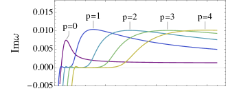
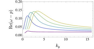
Figure 1: Growth rate $\Im\omega$ and frequency shift $\Re(\omega-p)$ relative to the associated harmonic $p$ of the Larmor frequency for various eigenmodes of (10) for $\kappa_{T}=0.34$, $\kappa_{n}=0.23$, ${k_{\perp}}=k_{y}$, $k_{z}=0.025$; $p=0$ represents the gyrokinetic slab ITG mode, $p>0$ non-gyrokinetic unstable IBWs.

Critical gradients of ion Bernstein waves

In principle, unstable non-gyrokinetic modes can exist for arbitrary complex $\omega$, since the real and imaginary part of (10) can always be satisfied by choosing suitable real parameters $\kappa_{n},\kappa_{T}$, which in general turn out to be of order of the inverse Larmor radius. However, we would like to know under which conditions there are also low gradient non-gyrokinetic instabilities with $|k_{y}\kappa_{n}|,|k_{y}\kappa_{T}|\ll 1$ and $\omega$ arbitrarily close to the Larmor resonances – similar to the well-known gradient threshold for the (slab) gyrokinetic ITG modes at very small frequencies. Cauchy’s argument principle [9] implies that threshold parameters for the instability fulfill the dispersion relation exactly at real $\omega$. Conversely, stability is implied, if no such threshold parameters can be found.

Due to the Gaussian dependence of the imaginary part of $Z$, it can be neglected in all but one Larmor resonance $p$ for frequencies close to the gyro resonances, i.e., if $\delta\omega=(\omega-p)\ll 1$ and $|k_{z}|\ll 1$, the latter of which must be verified a posteriori. The imaginary part of (10,9) then turns into

$$[-\omega+k_{y}(\kappa_{n}+\kappa_{T}\partial_{T})]\frac{\Gamma_{p}(T{k_{\perp}}^{2})}{\sqrt{T}}e^{-\frac{\delta\omega^{2}}{2{k_{z}}^{2}T}}=0,$$ (11)

equivalent to

$$-\frac{\omega}{k_{y}}+\kappa_{n}+\left(\frac{\delta\omega^{2}}{k_{z}^{2}}+\frac{d\ln\Gamma_{p}({k_{\perp}}^{2})}{d\ln{k_{\perp}}}-1\right)\frac{\kappa_{T}}{2}=0,$$ (12)

while the real part of the dispersion relation is

$$\chi_{\text{nr}}+\left[-\omega+{k_{y}}(\kappa_{T}\partial_{T}+\kappa_{n})\right]\frac{\Gamma_{p}(T{k_{\perp}}^{2})}{|{k_{z}}|\sqrt{2T}}Z\left(\frac{\delta\omega}{|{k_{z}}|\sqrt{2T}}\right)=0$$ (13)

with the weakly $\omega$-dependent non-resonant charge density response defined as

$$\chi_{\text{nr}}=-2+\left[-\omega+{k_{y}}(\kappa_{T}\partial_{T}+\kappa_{n})\right]\sum_{q\in\mathds{Z},q\neq p}\frac{\Gamma_{q}(T{k_{\perp}}^{2})}{|{k_{z}}|\sqrt{2T}}Z\left(\frac{\omega-q}{|{k_{z}}|\sqrt{2T}}\right).$$ (14)

In the limit $\omega=p$, $k_{z}\rightarrow 0$ and small gradients, the constant term dominates the expression for $\chi_{\text{nr}}$. Direct numerical inspection for varying $p$ and arbitrary ${k_{\perp}}$ shows that $|\chi_{\text{nr}}+2|<1.29|1-k_{y}\kappa_{n}/\omega|+0.52|k_{y}\kappa_{T}/\omega|$ for $p\neq 0$, and $|\chi_{\text{nr}}+2|<|k_{y}\kappa_{T}|$ for $p=0$. Hence, for sufficiently small gradients $\chi_{\text{nr}}<0$, and more specifically $-2.3\lesssim\chi_{\text{nr}}\lesssim-0.7$. Solving (11) for $\kappa_{n}$ and inserting it into (13) cancels the plasma dispersion function,

$$\chi_{\text{nr}}+\frac{1}{2}\frac{\delta\omega}{k_{z}^{2}}\kappa_{T}k_{y}\Gamma_{p}({k_{\perp}}^{2})=0,$$ (15)

where the identity $Z^{\prime}(x)=-2(1+xZ(x))$ has been used.

Solving (15) for $k_{z}^{2}$ one can replace $k_{z}$ as a parameter by $\delta\omega$ provided that $\delta\omega\,k_{y}\kappa_{T}\chi_{\text{nr}}<0$. With this, (11) results in

$$-\frac{p}{k_{y}}+\kappa_{n}+\left(\frac{d\ln\Gamma_{p}({k_{\perp}}^{2})}{d\ln{k_{\perp}}}-1\right)\frac{\kappa_{T}}{2}-\delta\omega\left(1+\frac{\chi_{\text{nr}}}{\Gamma_{p}}\right)=0.$$ (16)

Fixing the signs of $k_{y},\kappa_{T}$ to be positive, the sign of the term proportional to $\delta\omega$ is always positive for low gradients, since $\chi_{\text{nr}}<-\Gamma_{p}$, because $\Gamma_{0}\leq 1$, $\Gamma_{p}<0.25/p$ for any ${k_{\perp}}$. Thus, the existence of a threshold requires the rest of (16) to be negative, in other words,

$$\kappa_{n}<\frac{p}{k_{y}}+\left(1-\frac{d\ln\Gamma_{0}({k_{\perp}}^{2})}{d\ln{k_{\perp}}}\right)\frac{\kappa_{T}}{2}.$$ (17)

For the gyrokinetic ITG mode $p=0$, and the standard threshold condition results. For the instability of non-gyrokinetic modes (17) requires $p>0$ and no conditions on the gradients themselves besides their assumed smallness, and the condition that $\kappa_{T}\neq 0$, since otherwise (15) cannot be solved for $k_{z}^{2}$. Then, for an arbitrarily small $\delta\omega$ a marginally stable threshold mode exists at small $k_{y},{k_{\perp}}$, since

$$\frac{k_{y}\chi_{\text{nr}}}{\Gamma_{p}({k_{\perp}}^{2})}=-O(k_{y}^{1-2p})\rightarrow-\infty\mbox{ for }k_{y}={k_{\perp}}\rightarrow 0$$ (18)

and another one at large ${k_{\perp}}$ at fixed $k_{y}$, since

$$\frac{k_{y}\chi_{\text{nr}}}{\Gamma_{p}({k_{\perp}}^{2})}=-O({k_{\perp}})\rightarrow+\infty\mbox{ for }{k_{\perp}}\rightarrow\infty,k_{y}=const.$$ (19)

Since according to (15) in both limits ${k_{z}}\rightarrow 0$, the initial assumption of a single resonance contributing to the imaginary part of the ion response is justified. On the other hand, if (17) does not hold, (16) has no valid solutions in ${k_{\perp}}$ and $\delta\omega$, and hence there are no real solutions for any $\omega$, $k_{z}$, $k_{y}$, and ${k_{\perp}}$ for the system of equations (11,13) and therefore according to Cauchy’s argument theorem [9] there are no low-gradient instabilities close to the resonance in the system.

Since the condition $p>0$ only concerns the sign of the phase velocity and not the gradients themselves, the non-gyrokinetic high frequency IBW instabilities occur even when the gyrokinetic ITG modes are ruled out by the thresholds – the IBWs just require a non-zero temperature gradient.

Solving the equations (15,16) numerically for $\delta\omega$ and $\kappa_{T}$ without restriction to weak gradients (Fig. 2) confirms the theory. As expected, low frequency slab ITG modes at $p=0$ show an increasing temperature gradient threshold with increasing density gradient. The ratio of temperature to density gradient has to be $\eta=\frac{\kappa_{T}}{\kappa_{n}}\gtrapprox 0.9$ at the most unstable wavenumber. In contrast, the graph for $p=1$, but not $p<0$, shows that the Bernstein instability can occur for very small temperature gradients. Interestingly, in the H-mode typically $\eta=0.6-1.2$ [10], which should largely suppress the gyrokinetic ion temperature gradient mode. In all cases the critical temperature gradient increases with the density gradient.

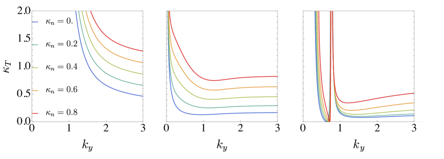
Figure 2: Critical temperature gradient for low frequency ITG mode (middle) and first harmonic IBWs with $p=-1$ (left) and $p=1$ (right) for varying $\kappa_{n}$ at $k_{z}=0.025$.

As for the growth rates at fixed temperature gradient (Fig. 3) one sees that in contrast to $p=0$ the modes with $p>0$ are further destabilized with increasing density gradient. The ITG instability is stabilized for $\eta<1.1$, while the high frequency IBW have the maximum growth rate at $\eta<1$, again suggesting their relevance in the H-mode regime, possibly as part of the residual transport.

Figure 3: Growth rate of ITG ($p=0$) and IBW ($p\neq 0$) instability as a function of $\frac{1}{\eta}=\frac{\kappa_{n}}{\kappa_{T}}$ for fixed temperature gradient $\kappa_{T}=0.36$ and $k_{y}={k_{\perp}}=2$, $k_{z}=0.025$.

6D turbulence simulations

Having executed extensive linear and nonlinear benchmarking simulations [11, 12] with BSL6D to solve (1), confirming the dispersion relation and reproducing results analogous to [3], for brevity we report only on a characteristic turbulence run showing the most relevant features of the high-frequency turbulence.

Since there is no equivalent to the gyrokinetic flux-tube scenario for the non-gyrokinetic equations without the additional approximation (4), we use periodic boundary conditions. The ion distribution function $f({\bm{x}},{\bm{v}})$ is initialized with a Maxwellian $f_{0}=f_{M}(n,T)$ with a background density and temperature profile similar to (2),

$$n=1+g_{n}\sin\frac{2\pi x_{gc}}{L_{x}}+\text{ran}(\bm{r}_{gc}),\;T=1+g_{T}\sin\frac{2\pi x_{gc}}{L_{x}},$$ (20)

to eliminate spurious transient gyro-oscillations, with the addition of a small white noise density perturbation $\text{ran}(\bm{r}_{gc})$. The profile amplitudes have been set to $g_{T}=0.6$ and $g_{n}=0.49$, resulting in the maximum inverse gradient lengths $\max(\kappa_{T})=0.375$ and $\max(\kappa_{n})=0.28$, to specifically render both slab ITG and IBWs unstable. (For lower temperature gradient the ITG would be completely suppressed.)

The computation has been carried out in a phase space region covering the spatial domain $L_{x}\times L_{y}\times L_{z}=4\pi\times 2\pi\times 80\pi$ and the velocity domain $[-4,4]^{3}$ using a computational grid of dimensions $64\times 32\times 16\times 32\times 32\times 16$ for the phase space coordinates $(x,y,z,v_{x},v_{y},v_{z})$. $N_{t}=1250000$ steps have been carried out with the time step $\Delta t=0.008$ up to the end time $t_{e}=10000$, using $150000$ core hours on the Intel Xeon 8160 CPUs of the Cineca Marconi cluster. In the following, band pass filters have been used diagnostically to separate fluctuation frequencies in the range $|\omega-p|<1/2$ for integer $p$.

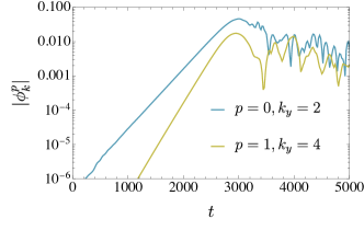
Figure 4: Amplitude of dominant Fourier modes in $y$-direction at their local maxima, $x=5.6$ and $x=3.6$ at $k_{z}=0.025$ for gyrokinetic modes $p=0$ and the first Larmor harmonic $p=1$.

The simulation starts with the linear growth followed by the turbulent saturation of the instabilities. The amplitude of the dominant gyrokinetic and non-gyrokinetic modes are shown in Fig. 4. Their respective growth rates (indexed “BSL6D”),

 $\gamma_{\mathrm{BSL6D}}$ $\gamma_{\mathrm{ana}}$ $p=0$ 0.0040 0.0024 $p=1$ 0.0062 0.0070

are consistent with the ones (indexed “ana”) computed from the dispersion relation (10) using the local gradients $\kappa_{n}=0.25$, $\kappa_{T}=0.34$, and $(k_{x},k_{y},k_{z},p)$ equal to $(0.5,2,0.025,0)$ and $(3,4,0.025,1)$, respectively. An exact agreement cannot be expected, since the inherently non-local setup of the simulation prohibits eigenmodes with a well defined wavenumber $k_{x}$.

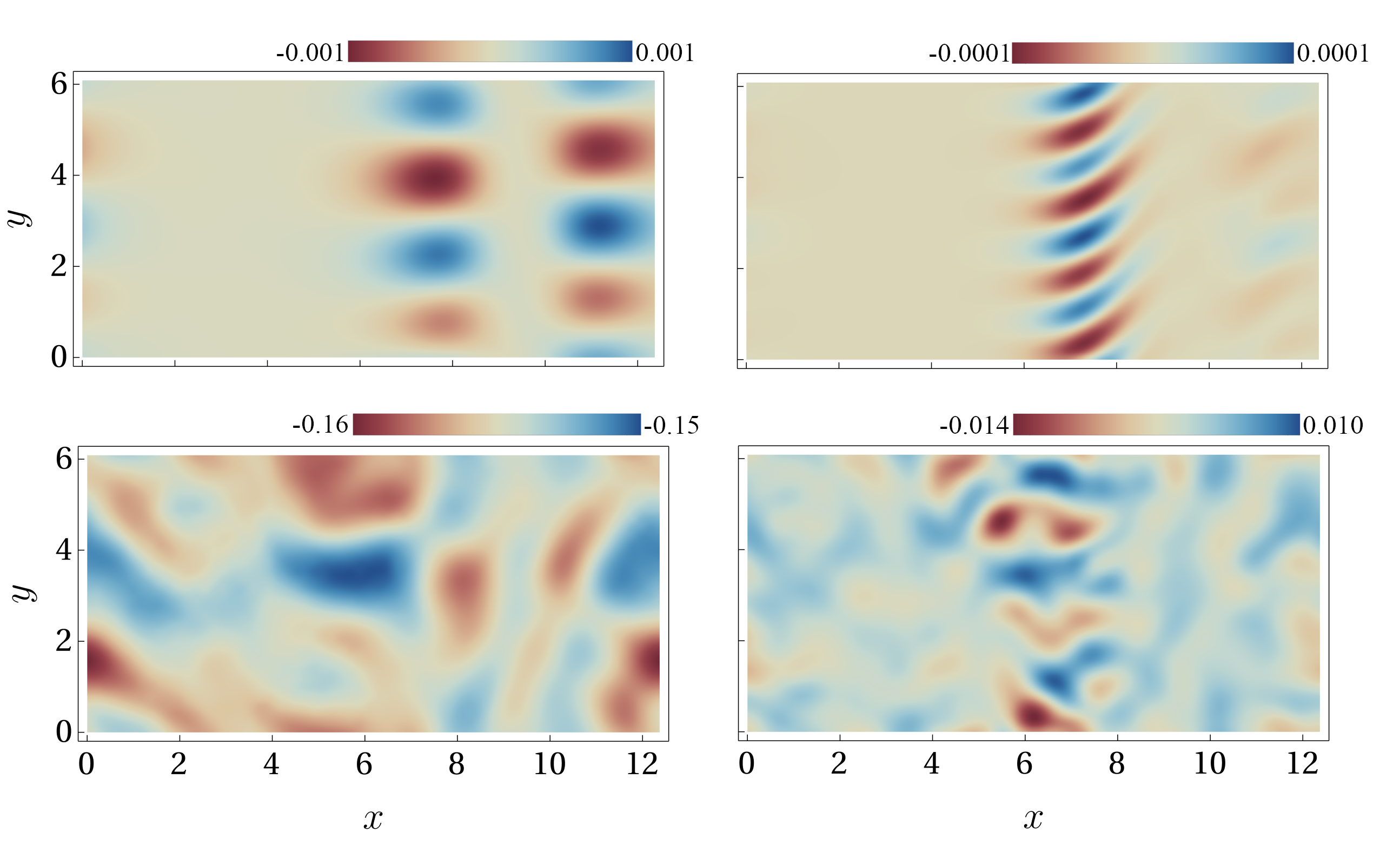
Figure 5: Cross sections of potential fluctuations $\phi$ for $p=0$ (left column) and $p=1$ (right column) at fixed $z$ and $t=1500,5500$ (rows).

The progression to turbulence is also observable in 2D cross sections of the electric potential (Fig. 5) (for a movie see [13]). At $t=1500$ the simulation is in the linear phase and a clear mode structure of the ITG and IBW (with larger wavenumbers) is visible. At $t=5500$ the potential indicates nonlinear ITG/IBW turbulence.

While the total energy flux across the magnetic field in the 6D turbulence simulations necessarily contains contributions from the Poynting flux [14] and genuinely non-gyrokinetic terms, the dominant component in the case at hand still comes from the $\bm{E}\times\bm{B}$ flow of the internal ion energy density $\epsilon=\int fv^{2}d^{3}v/2$, namely $\bm{q}_{\perp}\approx\epsilon\hat{z}\times\nabla\phi.$ Despite their high wavenumbers, the non-gyrokinetic $p\neq 0$ IBW components of the potential fluctuations are significant in comparison to the ITG fluctuations. The transport of the former even exceeds the one of the latter (Fig. 6) in the turbulent phase, although the mixing length argument would suggest a much lower transport due to the high wavenumber. We believe this to be at least partially due to the (necessarily) non-local setup, which tends to damp long wavelengths.

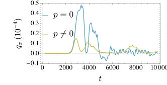
Figure 6: Comparison between low frequency modes $p=0$ and IBWs ($p\neq 1$) for potential amplitude $|\phi|$ (top) and internal ion energy flux $q_{x}$ (bottom), spatially averaged at $x=7.3$ and box-car averaged over $380$ time units.

Discussion

Using a novel 6D kinetic simulation code specifically designed for strongly magnetized plasmas we have shown that high frequency non-gyrokinetic instabilities (ion Bernstein waves, IBWs) can produce transport-relevant turbulence, even in competition to gyrokinetic ITG turbulence, which is usually exclusively considered in those plasmas. The simulations have been simplified by assuming electrostatic fields, adiabatic electrons and a homogeneous magnetic field. They refer therefore mostly to the ion turbulence component of low-$\beta$, high-gradient plasmas, where the magnetic fluctuations are small and the magnetic field inhomogeneities are unimportant compared to the plasma gradients. Nevertheless, the IBWs can be analytically shown to be unstable at arbitrarily low gradients and wavenumbers. They require only the presence of a temperature gradient, and not the excess of a temperature gradient threshold like the ITG modes.

Gradient lengths such as in the simulation detailed above, $\sim 3\rho_{i}$, are regularly encountered in the edge of tokamak H-mode discharges [10], where also the temperature gradients are typically below the ITG instability threshold, since $\eta=L_{n}/L_{T}\sim 0.6-1.2$. This, together with the potential breakdown of gyrokinetic theory for short gradient lengths and the lack of a satisfying explanation for the L/H-transition, suggests a full 6D treatment of turbulence to be very relevant to the edge region of magnetic confinement devices. In future work, more detailed electron physics and inhomogeneous, fluctuating magnetic fields will be included in such simulations. It seems likely that the inclusion of additional degrees of freedom would rather increase than decrease the intensity of the non-gyrokinetic modes.