Abstract

A topic of great current interest is Causal Representation Learning (CRL), whose goal is to learn a causal model for hidden features in a data-driven manner. Unfortunately, CRL is severely ill-posed since it is a combination of the two notoriously ill-posed problems of representation learning and causal discovery. Yet, finding practical identifiability conditions that guarantee a unique solution is crucial for its practical applicability. Most approaches so far have been based on assumptions on the latent causal mechanisms, such as temporal causality, or existence of supervision or interventions; these can be too restrictive in actual applications. Here, we show identifiability based on novel, weak constraints, which requires no temporal structure, intervention, nor weak supervision. The approach is based assuming the observational mixing exhibits a suitable grouping of the observational variables. We also propose a novel self-supervised estimation framework consistent with the model, prove its statistical consistency, and experimentally show its superior CRL performances compared to the state-of-the-art baselines. We further demonstrate its robustness against latent confounders and causal cycles.

1 INTRODUCTION

Causal discovery aims to learn causal interactions among observed variables in a data-driven manner (Pearl, 2000). The goal is to estimate a causal graph, also called an adjacency matrix, from passively observed data, with minimal assumptions. It plays an important role in a wide variety of fields, enabling fundamental insight into causal mechanisms latent in the data; importantly, this is possible without conducting expensive and time-consuming interventional experiments. However, the problem is ill-posed in general, and thus the main focus of causal discovery research is to find conditions where the causal graph can be uniquely determined (Andersson et al., 1997; Spirtes et al., 2001). A large number of studies have been conducted so far; they have basically found that imposing some asymmetricity into the model, such as nonlinearity or non-Gaussianity, enables its unique identification (Hoyer et al., 2008a; Peters et al., 2014; Shimizu et al., 2006, 2011; Zhang and Hyvärinen, 2009).

A crucial and implicit assumption of most causal discovery research is that we know exactly what constitutes the causal variables; in most cases, we implicitly assume that each observational variable corresponds to a single causal variable, i.e. a node in the causal graph. However, this is not necessarily true, for example when what is actually observed is raw, high-dimensional sensory data. Consider natural images: we do not really know in advance what kinds of objects are present, while the causal interactions should probably be modeled on the level of the objects. Therefore, in order to understand what kind of causal mechanism is generating such low-level sensory data, we also need to extract the “high-level” causal variables constructing the causal graph by performing representation learning (Bengio et al., 2013) simultaneously.

Nonlinear representation learning has its own problems of identifiability. Recent work has solved the identifiability problem in the context of Nonlinear Independent Component Analysis (NICA) by assuming temporal structure or an additional (conditioning) auxiliary variable (Hyvärinen and Morioka, 2016; Hyvarinen and Morioka, 2017; Hyvarinen et al., 2019; Klindt et al., 2021; Sprekeler et al., 2014). However, if the components are mutually independent, it seems impossible to model causal connections between them, and thus such theory is not directly applicable to this case. Thus, we need to go beyond independent components (Zhang and Hyvärinen, 2010; Khemakhem et al., 2020b) and build an explicit model of the dependencies resulting from their causal interactions.

Such simultaneous learning of the causal variables (representation learning) and their causal graph (causal discovery) has been a focus of intense attention recently, resulting is what is called as Causal Representation Learning (CRL) (Schölkopf et al., 2021). Since both of the two separate problems combined here are known to be ill-posed, CRL seems to be even more severely ill-posed, and much less is known on identifiability of CRL. Yet, finding identifiability conditions is crucial for its interpretability, applicability, and reproducibility. So far very limited frameworks were proposed, and many of them are based on heavy assumptions on the causal mechanisms, such as supervision or intervention on latent variables or causal graphs (Brehmer et al., 2022; Kivva et al., 2021; Shen et al., 2022; Yang et al., 2021), or temporal causality (dynamics) (Lachapelle et al., 2022; Lippe et al., 2022; Yao et al., 2022b, a).

Here, we propose a new model for CRL based on a novel approach assuming that the observed variables follow a certain grouping structure known a priori, as illustrated in Fig. 1c. Such grouping is common and naturally appears in many practical situations. For example, the variables could be grouped based on which measurement sensor they come from; or which time point or geographical location they are measured at. We further assume that the causal interactions are pairwise as in a Markov model of first order. Under these assumptions, we prove identifiability with much weaker, and very different, constraints than previous work. The model in particular is able to consider instantaneous causal relations rather than temporal (Granger) causality, while autoregressive (AR) dynamics are further contained as a special case. Nor does our model assume any supervision or interventions. Our experiments on synthetic data as well as a realistic gene regulatory network dataset show that our framework can indeed extract latent causal variables and their causal structure, with better performance than the state-of-the-art baselines.

2 RELATED WORKS

The general form of the CRL problem can be defined as an estimation of a set of causally-related latent variables ${\mathbf{\bm{s}}}=[s_{1},\ldots,s_{D_{\mathcal{S}}}]^{\mathsf{T}}\in\mathbb{R}^{D_{\mathcal{S}}}$, or causal variables for short, together with their causal structure. We typically assume that the observed data ${\mathbf{\bm{x}}}\in\mathbb{R}^{D_{\mathcal{X}}}$ are obtained via an unknown observational mixing ${\mathbf{\bm{f}}}:\mathbb{R}^{D_{\mathcal{S}}}\rightarrow\mathbb{R}^{D_{\mathcal{X}}}$ as

$${\mathbf{\bm{x}}}={\mathbf{\bm{f}}}({\mathbf{\bm{s}}}),$$ (1)

where the latent causal variables $s_{1},\ldots,s_{D_{\mathcal{S}}}$ are not mutually independent but follow a causal model to be specified. Typically, the causal model would be a Structural Equation Model (SEM) (Shen et al., 2022; Yang et al., 2021) which has a well-defined causal semantics. However, as a kind of proxy one might use something simpler such as a Bayesian network (BN). It is usually assumed that ${\mathbf{\bm{f}}}$ is injective, so there may be more observed variables than the latent variables; $D_{\mathcal{X}}\geq D_{\mathcal{S}}$.

In this work we only consider the case of independent and identically distributed (i.i.d.) sampling, which means the different observations of ${\mathbf{\bm{x}}}$ are independent of each other and there is no time structure. This obviously implies the causal relations must also be instantaneous. Such a causal model is more generally applicable, and in strong contrast to a lot of previous work which strongly relies on temporal structure (Lachapelle et al., 2022; Li et al., 2020; Lippe et al., 2022, 2023; Yao et al., 2022b, a) (Fig. 1b).

CRL can be seen as a generalization of NICA and causal discovery, both of which are known to be ill-posed without any specific assumptions. NICA can actually be seen as a special case of CRL, where the latent variables follow the degenerate causal graph in the sense of not having any causal relations. Recent studies have shown that NICA can be given identifiability by assuming temporal structure (Hyvärinen and Morioka, 2016; Hyvarinen and Morioka, 2017; Hyvarinen et al., 2019; Klindt et al., 2021; Sprekeler et al., 2014), instead of i.i.d. sampling. On the other hand, causal discovery is also a special case of CRL, where the causal variables are observed directly. Many studies have shown that some kind of asymmetricity of the statistical causal model enables the identifiability (Hoyer et al., 2008a; Park and Raskutti, 2015; Peters et al., 2014; Shimizu et al., 2006, 2011; Zhang and Hyvärinen, 2009).

The CRL model thus violates the important assumptions of the both problems (mutual independence, non-i.i.d., and direct observability). The research goal of CRL is thus to find the practical conditions for the identifiability of the model. Some studies have shown the identifiability in the instantaneous causality case, but they require supervision or intervention on the causal variables (Ahuja et al., 2022a, b; Brehmer et al., 2022; Kivva et al., 2021; Shen et al., 2022; Yang et al., 2021) (Fig. 1a), which might be too restrictive in actual applications. Recently (Sturma et al., 2023) proposed a concept of grouping of variables for CRL, similarly to this study, while it is limited to linear causal model and linear observational mixing, and can identify the causal structure only between variables shared across all groups. A more detailed discussion about the related works are given in Supplementary Material F.

3 MODEL DEFINITION

Our basic idea is to impose some constraints on the observational model ${\mathbf{\bm{f}}}$, based on grouping of the observed variables, together with some Markov-like (pairwise) constraints on the causal interactions between the groups (Fig. 1c). Next we first define our observational model and then the causal model.

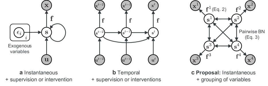
Figure 1: Comparison of the graphical models of major CRL frameworks whose goal is to estimate latent causal variables ${\mathbf{\bm{s}}}$ from the low-level observations ${\mathbf{\bm{x}}}$, usually with supervision or intervention $\mathbf{u}$. Our proposal in (c) is based on the grouping of variables (Eq. 2; $M=4$ groups here) and pairwise causal model (Eq. 3), and does not require any supervision or intervention, greatly generalizing the existing models.

Observation Model

As the original approach in our model, we assume that the observational mixing can be separated into $M>1$ non-overlapping groups. After appropriate permutations of the elements of ${\mathbf{\bm{s}}}$ and ${\mathbf{\bm{x}}}$ without loss of generality, we assume that the observation model Eq. 1 can be expressed as

$${\mathbf{\bm{x}}} =\begin{bmatrix}{\mathbf{\bm{x}}}^{1},&\ldots,&{\mathbf{\bm{x}}}^{M}\end{bmatrix}={\mathbf{\bm{f}}}(\begin{bmatrix}{\mathbf{\bm{s}}}^{1},&\ldots,&{\mathbf{\bm{s}}}^{M}\end{bmatrix})$$

$$=\begin{bmatrix}{\mathbf{\bm{f}}}^{1}({\mathbf{\bm{s}}}^{1}),&\ldots,&{\mathbf{\bm{f}}}^{M}({\mathbf{\bm{s}}}^{M})\end{bmatrix},$$ (2)

where ${\mathbf{\bm{x}}}^{m}=[x_{1}^{m},\ldots,x_{{d_{\mathcal{X}}^{m}}}^{m}]^{\mathsf{T}}\in\mathbb{R}^{{d_{\mathcal{X}}^{m}}}$ and ${\mathbf{\bm{s}}}^{m}=[s_{1}^{m},\ldots,s_{{d_{\mathcal{S}}^{m}}}^{m}]^{\mathsf{T}}\in\mathbb{R}^{{d_{\mathcal{S}}^{m}}}$ are the $m$-th group of the observational and latent variables respectively. Each element of the latent and the observational variables belongs to only one of the groups with index in ${\mathcal{M}}=\{1,\ldots,M\}$, which means that the $m$-th observational group ${\mathbf{\bm{x}}}^{m}$ is generated only as a function of ${\mathbf{\bm{s}}}^{m}$, without any observational contaminations from the other groups: in other words, ${\mathbf{\bm{x}}}^{m}={\mathbf{\bm{f}}}^{m}({\mathbf{\bm{s}}}^{m})$. The number of variables in a group can be different across groups. We usually denote the group index as a superscript, which should not be confused with an exponent; the element index as denoted by a subscript. Note that when $M=1$ this model corresponds to the general CRL (Eq. 1), and when $M=D$ this model simply leads to the ordinary causal discovery problem without observational mixing.

Illustrative Example 1: Causally Related Sensor Measurements

The most intuitive example would be where $m$ is a sensor index. Data is then obtained from a set of $M$ sensors, each measuring different but causally-related multidimensional physical quantities ${\mathbf{\bm{x}}}^{m(n)}\in\mathbb{R}^{d_{\mathcal{X}}^{m}}$ for each sample $n$. For example, in single-cell multiomics data (Burkhardt et al., 2022), each cell ($n$) could be measured to give chromatin accessibility (DNA) as ${\mathbf{\bm{x}}}^{1(n)}$, gene expressions (RNA) as ${\mathbf{\bm{x}}}^{2(n)}$, and protein levels as ${\mathbf{\bm{x}}}^{3(n)}$. These are all multi-dimensional quantities representing causally-interacting latent high-level features $\{{\mathbf{\bm{s}}}^{m}\}_{m}$. There exist many other possible applications consistent with this observational model; e.g., multimodal biomedical data (Acosta et al., 2022), simultaneous measurements of brain and behavior (Hebart et al., 2023), climate monitoring sensor networks (Longman et al., 2018), and so on, where $m$ corresponds to sensor modalities or locations.

Illustrative Example 2: Causal Dynamics

Although we focus on independent data samples rather than dynamics, our model can also implement dynamics with dependency across time by simply defining the group-index $m$ as time-index $t$ (see Figs. 1b and c). We then obtain low-level observations ${\mathbf{\bm{x}}}^{t}$ (such as images) from high-level latent causal process composed of multidimensional variable ${\mathbf{\bm{s}}}^{t}$ through time-dependent mixing model ${\mathbf{\bm{x}}}^{t}={\mathbf{\bm{f}}}^{t}({\mathbf{\bm{s}}}^{t})$ for each time point $t$. In this case, our model gives a generic form of a time series model, which is actually more general compared to some existing studies of CRL based on dynamics (Lachapelle et al., 2022; Lippe et al., 2022; Yao et al., 2022b, a) in the sense that the mixing function ${\mathbf{\bm{f}}}^{t}$ changes as a function of time $t$, which can happen in many practical situations (such as changes of the camera angle capturing the images). In this case, we assume we observe the same time-series many times, i.e. we have ${\mathbf{\bm{x}}}^{t(n)}$ where $n$ is the index of the time series realization (e.g., capturing images with multiple sequences $n$ with the same transition of camera angles across $t$ every time).

Causally Structured Latent Variable

Next we model the causal structure of the latent variables based on a BN, which is in particular pairwise, in the spirit of first-order Markov process or Markov random field. Denote by $\phi(\cdot,\cdot)$ potential functions representing causal relations between two variables. Further, denote by $\bar{\phi}^{m}$ group-wise potential functions representing causal relations inside a group, i.e. between the elements of ${\mathbf{\bm{s}}}^{m}$, which are not restricted in any way. We assume that the joint distribution $p({\mathbf{\bm{s}}})$ is factorized as

$$p({\mathbf{\bm{s}}})\propto \left[\prod_{m\in{\mathcal{M}}}\exp\left(\bar{\phi}^{m}({\mathbf{\bm{s}}}^{m})\right)\right]$$ (3)

$$\times\prod_{m\neq m^{\prime}}\prod_{(a,b)\in{{\mathcal{V}}_{\mathcal{S}}^{m}}\times{{\mathcal{V}}_{\mathcal{S}}^{m^{\prime}}}}\exp\left(\lambda_{ab}^{mm^{\prime}}\phi(s_{a}^{m},s_{b}^{m^{\prime}})\right),$$

where we denote the set of indices of the latent variables belonging to the $m$-th group by ${{\mathcal{V}}_{\mathcal{S}}^{m}}$ ($|{{\mathcal{V}}_{\mathcal{S}}^{m}}|={d_{\mathcal{S}}^{m}}$). The idea is to have a model of dependencies between variables which is so general that the estimation of the representation is not biased towards independent components. The variables in one group ${\mathbf{\bm{s}}}^{m}$ can causally affect all variables on the other groups $m^{\prime}\neq m$, in a complex manner, thus breaking any independence of variables. Importantly, potential functions composing of more than two variables do not exist across groups. The coefficient $\lambda_{ab}^{mm^{\prime}}\in\mathbb{R}$ modulates the strength of the causal relation $s_{a}^{m}\rightarrow s_{b}^{m^{\prime}}$, which is constantly zero if $s_{a}^{m}$ is not a direct causal parent of $s_{b}^{m^{\prime}}$. The sets of the coefficients $\mathbf{\bm{L}}=\{\mathbf{\bm{L}}^{mm^{\prime}}\}_{(m,m^{\prime})},\mathbf{\bm{L}}^{mm^{\prime}}=(\lambda_{ab}^{mm^{\prime}})_{a\in{{\mathcal{V}}_{\mathcal{S}}^{m}},b\in{{\mathcal{V}}_{\mathcal{S}}^{m^{\prime}}}}$ can be interpreted as (group-pair-wise) weighted adjacency matrices. Note that Eq. 3 just represents the factorization of the joint distribution and does not incorporate any causal directional assumptions between variables. We thus need some additional assumptions for the identifiability of this factorization model as a causal model as shown in Theorems below, similarly to causal discovery based on BN. As a special case, we can further consider a factorization of $\phi$, which represents exponential-family (additive) causal models (Supplementary Material A), which are more interpretable.

Illustrative Example 1: Causally Related Sensor Measurements

In the single-cell multiomics example, the model says there are causal relations between the groups, which can be consistent with what is known as the central dogma in molecular biology; DNA (${\mathbf{\bm{x}}}^{1}$) $\rightarrow$ RNA (${\mathbf{\bm{x}}}^{2}$) $\rightarrow$ Protein (${\mathbf{\bm{x}}}^{3}$). Our model considers that they are interacting on the high-level latent space $\{{\mathbf{\bm{s}}}^{m}\}_{m}$, such as something related to transcription factors, probabilistically, in a pairwise manner.

Illustrative Example 2: Causal Dynamics

In the temporal dynamics example above, it is natural to have causal relations across the time-index $t$ (which is the same as the group-index $m$). Our model extends the previous models in the sense that any pairs of latent variables can be causally related across time (no sparseness is required unlike Lachapelle et al. (2022)). It is also worth mentioning that temporal causality from the past to the present is a special case in our model since our model (Eq. 3) does not restrict the causal directions between the groups.

4 IDENTIFIABILITY OF REPRESENTATION LEARNING

Based on the grouping assumption of the observational model (Eq. 2), together with the assumptions on pairwise inter-group dependencies of the variables (Eq. 3), we can prove new identifiability results of the CRL model. In this section, we first consider identifiability of the latent variables. We assume that each mixing function ${\mathbf{\bm{f}}}^{m}$ is invertible and $C^{2}$ diffeomorphism (thus ${d_{\mathcal{S}}^{m}}={d_{\mathcal{X}}^{m}}$; we later discuss the case ${d_{\mathcal{S}}^{m}}<{d_{\mathcal{X}}^{m}}$). Apart from that, we do not assume any parametric form for each ${\mathbf{\bm{f}}}^{m}$. We consider the situation where the support of the distribution of each variable is connected (i.e. an interval), and without loss of generality, the same across all variables, denoted as $\bar{\mathcal{S}}$. We denote $\phi^{112}(x,y)=\frac{\partial^{3}}{\partial x^{2}\partial y}\phi(x,y)$, $\phi^{122}(x,y)=\frac{\partial^{3}}{\partial x\partial y^{2}}\phi(x,y)$, and $\phi^{12}(x,y)=\frac{\partial^{2}}{\partial x\partial y}\phi(x,y)$. Those functions are said to be uniformly dependent (Definition 2 in Supplementary Material B) if the set of zeros of the function does not contain any open subset in the support of the input distribution. For a variable $s_{a}^{m}$, we call $s_{b}^{m^{\prime}}$ in some other group a neighbor if either or both of the adjacency coefficients $\lambda_{ab}^{mm^{\prime}}$ and $\lambda_{ba}^{m^{\prime}m}$ are non-zero. The identifiability condition is then given in the following Theorem, proven in Supplementary Material B;

Theorem 1.

Assume the generative model given by Eqs. 2 and 3, and also the following:

1. (Causal graph) For every group $m$ of interest, each variable has a (at least one) neighbor in some other group, and the collection of inter-group adjacency matrices $\bar{\mathbf{\bm{L}}}^{m}$ given below has full row-rank after removing all-zero rows:

   $$\bar{\mathbf{\bm{L}}}^{m}=\begin{bmatrix}\mathbf{\bm{L}}^{m1},&\ldots,&\mathbf{\bm{L}}^{mM}\\ (\mathbf{\bm{L}}^{1m})^{\mathsf{T}},&\ldots,&(\mathbf{\bm{L}}^{Mm})^{\mathsf{T}}\end{bmatrix},$$ (4)

2. (Causal function) $\phi^{12}$, $\phi^{112}$, and $\phi^{122}$ have uniform dependency, and for any open subset $B$ of $\bar{\mathcal{S}}$, there exist some $z_{1}\neq z_{2}\in\bar{\mathcal{S}}$ such that any of the following conditions does not hold for $\phi^{12}$: $\phi^{12}(s,z_{1})=c_{1}\phi^{12}(s,z_{2})$, $\phi^{12}(z_{1},s)=c_{2}\phi^{12}(z_{2},s)$, and $\phi^{12}(s,z_{1})=c_{3}\phi^{12}(z_{1},s)$ for all $s\in B$ with some constants $c_{1},c_{2},c_{3}\in\mathbb{R}$.

Then, for all $m$ satisfying A1, ${\mathbf{\bm{s}}}^{m}$ can be recovered up to permutation and variable-wise invertible transformations from the distribution of observations ${\mathbf{\bm{x}}}$.

The Assumption A1 requires each variable to have at least one neighbor in some other group, and the dependency needs to be distinct across variables (rows) and causal directions (upper and lower halves), as expressed by the full row-rank condition. Note that A1 does not require the causal graph to be directed as in Theorem 3 given below, though requires it to be asymmetric. Note also that the variables need to have neighbors only on some of the other groups but not on all of them; e.g. in practice, groups somehow “near-by” in space or time. This condition can be evaluated separately for each group $m$; we cannot identify the latent variables of the groups not satisfying A1, while they do not affect the identifiability of the other groups.

The Assumption A2 requires sufficient dependency of the cross-derivatives of $\phi$ on their inputs, and $\phi^{12}$ to be non-factorizable (the first two conditions) and asymmetric (the last condition). This assumption does not allow linear Gaussian SEMs, where $\phi(x,y)=xy$ (Supplementary Material A) and thus $\phi^{112}$ and $\phi^{122}$ are constantly zeros and $\phi^{12}$ is symmetric, which is consistent with the well-known result of causal discovery (Hoyer et al., 2008a; Peters et al., 2014). Although this also excludes some causal models which do not satisfy the non-factorizability (e.g., exponential family causal model with model order one, where $\phi(x,y)=\alpha(x)\beta(y)$ with some scalar functions $\alpha$ and $\beta$; Supplementary Material A), we can give an alternative condition not requiring it, by some additional constraints on the causal graph (Proposition 1 in Supplementary Material C).

5 REPRESENTATION LEARNING ALGORITHM

We now propose a self-supervised estimation framework called Grouped Causal Representation Learning (G-CaRL). Again, we start by learning the representation, i.e. learning to invert the mixing functions ${\mathbf{\bm{f}}}^{m}$. To this end, we propose a new contrastive learning method where the pretext task is to discriminate (classify) the following two datasets obtained from the same observations:

$${\mathbf{\bm{x}}}^{(n)}=\begin{bmatrix}{\mathbf{\bm{x}}}^{1(n)},&\ldots,&{\mathbf{\bm{x}}}^{M(n)}\end{bmatrix}$$

$$\text{vs.}\quad{\mathbf{\bm{x}}}^{(n_{\ast})}=\begin{bmatrix}{\mathbf{\bm{x}}}^{1(n_{\ast}^{1})},&\ldots,&{\mathbf{\bm{x}}}^{M(n_{\ast}^{M})}\end{bmatrix}$$ (5)

where $n$ indicates the sample index, while $n_{\ast}^{m}$ is a shuffled index, generated in practice by randomly selecting a sample index separately for each group $m$ (note that different groups have different sample indices in ${\mathbf{\bm{x}}}^{(n_{\ast})}$). We then learn a nonlinear logistic regression (LR) system which discriminates the two classes, using a cross-entropy loss with a specific form of the regression function with

$$r({\mathbf{\bm{x}}})=c+\sum_{m\in{\mathcal{M}}}\bar{\psi}^{m}({\mathbf{\bm{h}}}^{m}({\mathbf{\bm{x}}}^{m}))$$ (6)

$$+\sum_{m\neq m^{\prime}}\sum_{(a,b)\in{{\mathcal{V}}_{\mathcal{S}}^{m}}\times{{\mathcal{V}}_{\mathcal{S}}^{m^{\prime}}}}w_{ab}^{mm^{\prime}}\psi(h_{a}^{m}({\mathbf{\bm{x}}}^{m}),h_{b}^{m^{\prime}}({\mathbf{\bm{x}}}^{m^{\prime}})),$$

where ${\mathbf{\bm{h}}}^{m}:\mathbb{R}^{{d_{\mathcal{X}}^{m}}}\rightarrow\mathbb{R}^{{d_{\mathcal{S}}^{m}}}$ is a group-wise (nonlinear) feature extractor, $h_{a}^{m}$ is the $a$-th element of ${\mathbf{\bm{h}}}^{m}$, $\bar{\psi}^{m}:\mathbb{R}^{{d_{\mathcal{S}}^{m}}}\rightarrow\mathbb{R}$ and $\psi:\mathbb{R}^{2}\rightarrow\mathbb{R}$ are scalar-valued nonlinear functions, and $w_{ab}^{mm^{\prime}}$ and $c\in\mathbb{R}$ are weight and bias parameters. The observational grouping indices are assumed to be given in advance, while we only need the information of the size of groups ${d_{\mathcal{S}}^{m}}$ for the latent variables. The nonlinear functions are assumed to have universal approximation capacity (Hornik et al., 1989), and would typically be learned as neural networks. Any optimization method can be used to minimize the loss, though the theorem below assumes it gives the optimal solution without getting stuck in a local optimum. After the convergence, we obtain the following consistency Theorem, proven in Supplementary Material D;

Theorem 2.

Assume the same as those in Theorem 1, and also:

1. (Learning) We train a nonlinear LR system (Eq. 6) with universal approximation capability to discriminate two datasets ${\mathbf{\bm{x}}}^{(n)}$ and ${\mathbf{\bm{x}}}^{(n_{\ast})}$ (Eq.5).

2. (${\mathbf{\bm{h}}}$) The functions ${\mathbf{\bm{h}}}^{m}$ are $C^{2}$ diffeomorphisms.

Then, for all $m$ satisfying A1, in the limit of infinite samples $n$, the function ${\mathbf{\bm{h}}}^{m}({\mathbf{\bm{x}}}^{m})$ gives the latent variables on the $m$-th group ${\mathbf{\bm{s}}}^{m}$, up to permutation and variable-wise invertible transformations.

Interestingly, although this learning framework may not seem to be related to CRL at first sight, this theorem actually shows that learning the correct representation is achieved by learning the functions ${\mathbf{\bm{h}}}(\cdot)$ through the optimization of the regression function Eq. 6. This Theorem is basically based on the well-known fact that the regression function of an LR gives the posterior probability of one of the two classes (Eq. 5) after the training (Gutmann and Hyvärinen, 2012). Crucially, the group-wise shuffling breaks the causal relations between groups in ${\mathbf{\bm{x}}}^{(n_{\ast})}$, which means for the LR to discriminate the two datasets properly, it needs to capture the causal relations between groups in the latent space, by disentangling the observational mixing. Thanks to the compatibility of the factorization assumptions in the generative (Eq. 3) and in the regression model (Eq. 6), the optimal model is achievable only when ${\mathbf{\bm{h}}}^{m}$ essentially gives the inverse model of ${\mathbf{\bm{f}}}^{m}$, which automatically leads to CRL.

6 IDENTIFIABILITY OF CAUSAL DISCOVERY

Next, we consider how to learn the causal graph $\mathbf{\bm{L}}$. Thanks to the identifiability of the latent variables (Theorem 1) and the consistent estimation framework G-CaRL (Theorem 2), we can proceed by estimating it as a post-processing step, by just applying some existing causal discovery frameworks to the estimated latent variables; this is justified as far as their assumptions are consistent with our causal model (Eq. 3).

Nevertheless, it would be useful to fully integrate the causal discovery with the representation learning. In our model, this can be achieved by estimating the (weighted) adjacency coefficients $\lambda_{ab}^{mm^{\prime}}$ in the model (Eq. 3) from the observations in a data-driven manner, similarly to many causal discovery frameworks based on BN (Park and Raskutti, 2015; Park and Park, 2019b; Shimizu et al., 2006). We can actually achieve this by using the self-supervised algorithm in Section 5, where the adjacency coefficients $\{\lambda_{ab}^{mm^{\prime}}\}$ are learned as the weight parameters $\{w_{ab}^{mm^{\prime}}\}$ jointly with the inverse models ${\mathbf{\bm{h}}}^{m}$ in the regression function (Eq. 6). We omit the proof of the consistency since it can be easily shown by following those of Theorems 2 and 3 given below.

The identifiability of $\mathbf{\bm{L}}$ requires additional assumptions on $\mathbf{\bm{L}}$ and $\phi$, given in the following Theorem, proven in Supplementary Material E. It requires the causal relations between variables to be directed as in causal discovery, in contrast to Theorem 1; we call a causal relation between two variables $s_{a}^{m}$ and $s_{b}^{m^{\prime}}$ directed if only one of $\lambda_{ab}^{mm^{\prime}}$ and $\lambda_{ba}^{m^{\prime}m}$ has a non-zero value. It also requires each variable to have a co-parent and co-child in the same group, whose definition is given as: For a variable $s_{a}^{m}$, we call $s_{a^{\prime}}^{m}$ in the same group a co-parent (respectively co-child) of $s_{a}^{m}$ if it shares at least one child (respectively parent) $s_{b}^{m_{\ast}}$ on some other group ($m_{\ast}\in{\mathcal{M}}\setminus m$) with $s_{a}^{m}$. The indices $m_{\ast}$ and $b$ can be different across the co-parents and co-children.

Theorem 3.

Assume the same as those in Theorem 1, and also:

1. (Causal graph) The inter-group causal relations of variables are all directed, and for every group-pair $(m,m^{\prime})$ of interest, all variables in a group $m$ (and $m^{\prime}$) have both a co-parent and a co-child in the same group. In addition, any variables in the group $m$ (and $m^{\prime}$) can be reached from any other variables in the same group by moving from a variable to one of its co-parents, possibly by multiple hops (and similarly for co-children).

2. (Asymmetricity) There is no open subset $B$ of $\bar{\mathcal{S}}$ such that for all $x\neq y\in B$, it holds

   $$\phi^{12}(x,y)=c\phi^{12}(y,x)$$ (7)

   with some constant $c\in\mathbb{R}$.

Then, for all group-pairs $(m,m^{\prime})$ satisfying A1 and C1, $(\mathbf{\bm{L}}^{mm^{\prime}},\mathbf{\bm{L}}^{m^{\prime}m})$ are identifiable up to permutation of variables, linear scaling, and matrix transpose.

This theorem shows that we can identify the causal graphs $\mathbf{\bm{L}}$ from the data distribution up to linear scaling and matrix transpose (the permutations of variables are inevitable in CRL as typical in representation learning, and as shown in Theorem 1). This indeterminacy comes from the lack of specification of the functional form of $\phi$ in Eq. 3; a transposition of the adjacency matrix could be compensated by switching the order of the two arguments of $\phi$, and the scaling could be compensated by that of the function $\phi$.

The function $\phi$ is required to be asymmetric (C2), which is a natural assumption for causal discovery determining the causal directions in a data-driven manner.

The causal graph assumption (C1) is a special condition related to the grouping of variables (Eq. 2). It is required to remove the variable-wise nonlinear scaling indeterminacy of Theorem 1, and then to identify the causal graph up to a linear scaling. Although this would be relatively difficult to verify in advance since the graph structures are unknown in most cases, it would be fulfilled as long as the connections between groups are not sparse. One such example is causal dynamics (Illustrative example 2) having fully-connected autoregressive temporal causality to the subsequent time-point (group), since in this case all other variables in the same time-point (group) are both co-parents and co-children. The graph is required to be directed though not necessarily acyclic unlike in many causal discovery studies.

The assumptions on the causal graph (C1) and on the function $\phi$ have a trade-off relationship; by assuming additional constraints on $\phi$, the constraint on the causal graph (C1) can be weakened (see some variants of Theorem 3 in Supplementary Material E).

7 EXPERIMENTS

To validate the effectiveness of our framework, we compare it to several baselines in two simulation settings and one more realistic causal data. The baselines only include unsupervised frameworks with instantaneous causal interactions, since our experimental setting does not include supervision, intervention, nor temporal causality. Specifically, we used CausalVAE (Yang et al., 2021) in unsupervised setting, and the causal discovery frameworks DirectLiNGAM (Shimizu et al., 2011), NOTEARS (Zheng et al., 2018), NOTEARS-MLP (Zheng et al., 2020), GOLEM (Ng et al., 2020), PC (Spirtes and Glymour, 1991), CAM (Bühlmann et al., 2014), and CCD (Lacerda et al., 2008) (See Supplementary Material J). We first conduct experiments on a latent DAG model (Section 7.1), since many of the baselines assume DAGs. We then show applicability of G-CaRL to more a complex causal model having both directed cycles and latent confounders (Section 7.2). Lastly, we conduct an experiment with synthetic single-cell gene expression data in Section 7.3. The details of the experimental settings are given in Supplementary Material G, H, and I, respectively. Also see Supplementary Code for the implementation.

The settings are based on the generative model described in Sections 3 and 6. The number of groups ($M$) was fixed to 3, the number of variables was 10 for each group (${d_{\mathcal{S}}^{m}}=10,D_{\mathcal{S}}=30$) here, while we also show results with many different settings in the Supplementary Material. The latent variables are observed through nonlinear mixings randomly generated as a multilayer-perceptron (MLP) for each group. For those baseline methods which do not perform representation learning by themselves, we first applied $\beta$-VAE (Higgins et al., 2017) to achieve some level of disentanglement, though this may have little theoretical justification (we cannot use identifiable-VAE (Khemakhem et al., 2020a) since it requires weak supervision). For a fair comparison, we used the same architecture (group-wise disentanglement) for the encoders of CausalVAE and $\beta$-VAE as in the feature extractors ${\mathbf{\bm{h}}}^{m}$ of G-CaRL. We only evaluated the inter-group causal connections, since only those are identifiable in our model (Theorem 3).

7.1 Simulation 1: DAG

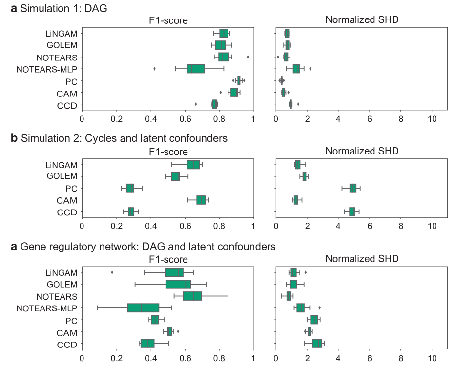
Figure 3: Evaluation of the causal discovery baselines applied directly on latent variables. (a) Simulation 1, (b) Simulation 2, and (c) Gene regulatory network recovery.

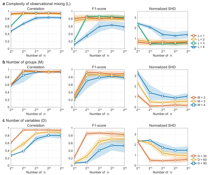
Figure 4: (Simulation 1) Estimation performances of the latent variables (Pearson correlation) and the causal structures (F1-score and normalized SHD) by the proposed framework G-CaRL, but different settings of (a) the complexity of the observation models (the number of MLP-layers $L$ of the observation function $\mathbf{\bm{f}}$), (b) the number of groups ($M$), and the (c) number of variables ($D_{\mathcal{S}}$), with changing the number of samples $n$. The values are the averages of 10 runs for each setting, and the shaded regions show the standard deviations. Fig. 2a corresponds to the case $L=3$, $M=3$, $D_{\mathcal{S}}=30$, and $n=2^{16}$.

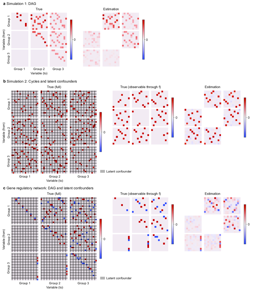
Figure 7: Example of the true causal structures (weighted adjacency matrices) and the estimations by G-CaRL (before causal direction determination and thresholding) in Simulation 1 (a), Simulation 2 (b), and the gene regulatory network recovery task (c). G-CaRL only identifies the inter-group-parts of the adjacency matrix, and thus the block-diagonal-parts are left unknown.

We first examined the performance with latent DAG models (Fig. 2a, Supplementary Fig. 7a shows some examples). The latent variables and the causal graphs were reconstructed reasonably well by G-CaRL, and with much higher performances than the baselines. Although CausalVAE is a CRL framework as well, its performances are significantly worse than ours, mainly due to the lack of supervision, which is supposed to be crucial for CausalVAE. The other baselines did not work well basically because of the poor disentanglement by $\beta$-VAE (Fig. 2a Correlation; note that they work reasonably well if they are applied directly to the latent variables as shown in Supplementary Fig. 3a). Supplementary Fig. 4 shows how the complexity of the mixing model ($L$), the number of variables $D_{\mathcal{S}}$, groups $M$, and sample size $n$ affect the performances; a higher $L$, $D_{\mathcal{S}}$, and $M$ make learning more difficult, while a larger $n$ makes it possible to achieve higher performances.

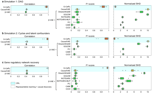
Figure 2: Comparison of CRL performance by the proposed G-CaRL and the baselines. The estimation performance is measured by Pearson correlation for the latent variables and by F1-score and normalized Structural Hamming Distance for the causal graphs. (a) Simulation 1 (basic DAG). (b) Simulation 2 (cycles and latent confounders). (c) Gene regulatory network recovery task.

7.2 Simulation 2: Cyclic Graphs with Latent Confounders

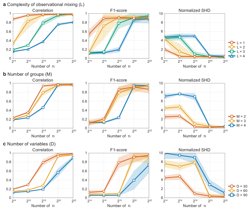
Figure 5: (Simulation 2) Estimation performances of the latent variables (Pearson correlation) and the causal structures (F1-score and normalized SHD) by the proposed framework G-CaRL, but different settings of (a) the complexity of the observation models (the number of MLP-layers $L$ of the observation function $\mathbf{\bm{f}}$), (b) the number of groups ($M$), and the (c) number of variables ($D_{\mathcal{S}}$), with changing the number of samples $n$. The values are the averages of 10 runs for each setting, and the shaded regions show the standard deviations. Fig. 2b corresponds to the case $L=3$, $M=3$, $D_{\mathcal{S}}=30$, and $n=2^{20}$.

To show the robustness of G-CaRL on more complex causal models, we next examined the performances with directed cycles and latent confounders with the same number as the observable variables (Fig. 2b; Supplementary Fig. 7b shows some examples). G-CaRL showed reasonably good performance even in this difficult condition, though it requires larger number of samples than Simulation 1 (Supplementary Figs. 4 and 5). On the other hand, the causal discovery baselines did not work well even when they were applied directly to the latent variables (Supplementary Fig. 3b). This result shows the effectiveness of the causal model of G-CaRL against the existence of causal cycles and latent confounders. Supplementary Fig. 5 shows the effects of the model complexity to the estimation performances, and they show a trend similar to Simulation 1.

7.3 Recovery of Gene Regulatory Network

We also evaluated G-CaRL on a more realistic causal data. We used synthetic single-cell gene expression data generated by SERGIO (Dibaeinia and Sinha, 2020), where each gene expression is governed by a stochastic differential equation (SDE) derived from a chemical Langevin equation, with activating or repressing causal interactions with the other genes. The causal graph was designed to be a DAG (as required of SERGIO) similarly to Simulation 1, but with latent confounders similarly to Simulation 2 (Supplementary Fig. 7c shows examples). We used the same setting for the observational mixings as those in the simulations above. G-CaRL showed the best performances among the baselines (Fig. 2c), which suggests the good applicability of G-CaRL to real datasets.

8 DISCUSSION

Our proposal extends the existing CRL models in many aspects; 1) the framework is unsupervised (only requires grouping of variables independent of the samples) rather than supervised (Brehmer et al., 2022; Kivva et al., 2021; Shen et al., 2022; Yang et al., 2021), 2) we consider instantaneous causality rather than temporal (Lachapelle et al., 2022; Lippe et al., 2022; Yao et al., 2022b, a), while the temporal causality is also contained as a special case, 3) the observational mixing can be group-dependent (or, time-dependent in the dynamics model, rather than time-invariant (Lachapelle et al., 2022; Lippe et al., 2022; Yao et al., 2022b, a)), 4) the latent variables can be nonlinearly causally related rather than linearly (Shen et al., 2022; Yang et al., 2021), nor is sparseness (Lachapelle et al., 2022) necessary, and 5) the causal graph can be cyclic, which is even more general than commonly used models for simple causal discovery.

Our model can be seen as a generalization of NICA, in the sense that 1) it allows causal relations between latent variables, rather than (conditional) mutual independence (Hyvarinen et al., 2019; Hälvä et al., 2021), and further, 2) the mixing function is time/group-dependent, which is completely new in NICA. Independently Modulated Component Analysis (Khemakhem et al., 2020b) was recently proposed as an extension of NICA to allow dependency across variables, but it requires an auxiliary variable unlike our framework. The crucial idea of our identifiability theorems is that we virtually use the variables on the other groups as auxiliary variables in the context of NICA. Importantly, instead of requiring additional auxiliary variables (supervision) for each sample as in those existing studies, this study nicely utilized the grouping structure to obtain them automatically.

Although we considered the case ${d_{\mathcal{X}}^{m}}={d_{\mathcal{S}}^{m}}$ for theoretical convenience, we can extend our framework to ${d_{\mathcal{X}}^{m}}\geq{d_{\mathcal{S}}^{m}}$. One approach is to assume that ${\mathbf{\bm{f}}}^{m}$ is injective (thus ${d_{\mathcal{X}}^{m}}\geq{d_{\mathcal{S}}^{m}}$) and $C^{2}$ diffeomorphism between $\mathcal{S}^{m}$ and ${\mathcal{X}}^{m}\in\mathbb{R}^{d_{\mathcal{X}}^{m}}$ which is a ${\mathcal{C}}^{2}$ differentiable manifold, as in Khemakhem et al. (2020b); Hälvä et al. (2021). Our proof can be adapted for that case following Khemakhem et al. (2020b); Hälvä et al. (2021). Another approach is to assume that ${d_{\mathcal{X}}^{m}}-{d_{\mathcal{S}}^{m}}$ variables are not causally related to any other groups, in which case our estimation framework would automatically ignore those variables.

Our estimation framework is based on the shuffling of the observational samples within each group, which is similar to some self-supervised learning frameworks heuristically proposed for multimodal-data (called Matching Prediction or Alignment Prediction; Zong et al. (2023)). However, most of them lack theoretical grounding, which may be provided by this study. The estimation based on shuffling is also similar to some NICA (Hyvarinen and Morioka, 2017; Hyvarinen et al., 2019), while our framework extends them to CRL.

Limitations

Our Theorems assume grouping of the observational mixing without any observational contamination across groups. Although it might sound restrictive, it should be satisfied in many practical applications as described in Illustrative examples above. Furthermore, the identifiability of the causal graphs only applies for connections across groups, and those within each group are left unknown. Nevertheless, since the latent variables are guaranteed to be identifiable, we can apply existing causal discovery framework for estimating them as a post-processing, as discussed in Section 6. In addition, the causal graph has the indeterminacy of matrix-transpose, though it can be resolved by some prior information about the $\phi$. Although the $\phi$ is assumed to be the same across all group-pairs for simplicity, it could be different across them, though it would require some additional assumptions.

9 CONCLUSION

This study proposed a new identifiable model for CRL, together with its self-supervised estimation framework G-CaRL. The new approach is the assumption of the grouping of the observational variables, which appears naturally in many practical applications such as multi-sensor measurements or time series. Such an assumption allowed us to significantly weaken any other assumptions required on the latent causal mechanisms in existing frameworks. In contrast to existing CRL models, our model does not require temporal structure (although it can use it as a special case), nor does it assume any supervision or interventions. Although our model restricts the inter-group causal relations of variables to pairwise, it allows nonlinearity and even cycles, which is more general than most of the causal discovery models. Numerical experiments showed better performances compared to the state-of-the-art baselines, thus making G-CaRL a promising candidate for real-world CRL in a wide variety of fields.

Acknowledgements

This research was supported in part by JST PRESTO JPMJPR2028, JSPS KAKENHI 22H05666 and 22K17956. A.H. was funded by a Fellow Position from CIFAR, and the Academy of Finland (project #330482).

Supplementary Materials for Causal Representation Learning Made Identifiable by Grouping of Observational Variables

Appendix A Parameterization of the Causal Function Based on Exponential Families

While the causal function $\phi$ in the factorization model (Eq. 3) is given in a general form, some more specific model would be useful for its practical applications and interpretability. One such way is to factorize the potential function $\phi$ as

$$\phi(x,y)={\mathbf{\bm{\eta}}}(x)^{\mathsf{T}}\mathbf{\bm{T}}(y),$$ (8)

where the factors ${\mathbf{\bm{\eta}}}(x)=[\eta_{1}(x),\ldots,\eta_{N}(x)]^{\mathsf{T}}$ and $\mathbf{\bm{T}}(y)=[T_{1}(y),\ldots,T_{N}(y)]^{\mathsf{T}}$ are some $N$-dimensional vector functions of a scalar input. We assume that factors ${\mathbf{\bm{\eta}}}$ and $\mathbf{\bm{T}}$ are differentiable almost surely. In addition, without loss of generality, we assume that they are minimal, whose definition is given below:

Definition 1.

(Minimality) We say that a function ${\mathbf{\bm{\alpha}}}:\mathbb{R}\rightarrow\mathbb{R}^{N}$ is minimal if for any open subset $\mathcal{X}$ of $\mathbb{R}$ the following is true:

$$\left(\exists\mathbf{\bm{\theta}}\in\mathbb{R}^{N}\mid\forall x\in\mathcal{X},\mathbf{\bm{\theta}}^{\mathsf{T}}{\mathbf{\bm{\alpha}}}(x)=\text{const.}\right)\implies\mathbf{\bm{\theta}}=\mathbf{\bm{0}}.$$ (9)

The minimality is similar to the linear independence of the elements, but stronger; minimality also forbids the existence of elements which only have differences of scaling and biases. Note that a non-minimal model can always be reduced to minimal one via a suitable transformation and reparameterization.

The point of this parameterization is that if the whole causal graph is acyclic, the conditional distribution of a variable can be represented by an (conditional) exponential family of order $N$, with sufficient statistics $\mathbf{\bm{T}}$ and the natural parameters given as additions of causal effects from the parents through the adjacency coefficients and the function ${\mathbf{\bm{\eta}}}$. More specifically, if the whole causal graph is acyclic and the intra-group causal relations are given in the pairwise form as in those of inter-groups, the conditional distribution of the variable $s_{a}^{m}$ is given, from Eqs. 3 and 8, by the following (conditional) exponential family of order $N$,

$$p(s_{a}^{m}\lvert\text{pa}(s_{a}^{m})) =\frac{1}{Z_{a}^{m}(\text{pa}(s_{a}^{m}))}h_{a}^{m}(s_{a}^{m})\exp\left(\sum_{s_{b}^{m^{\prime}}\in\text{pa}(s_{a}^{m})}\lambda_{ba}^{m^{\prime}m}{\mathbf{\bm{\eta}}}(s_{b}^{m^{\prime}})^{\mathsf{T}}\mathbf{\bm{T}}(s_{a}^{m})\right),$$

$$=\frac{1}{Z_{a}^{m}(\text{pa}(s_{a}^{m}))}h_{a}^{m}(s_{a}^{m})\exp\left(\tilde{{\mathbf{\bm{\eta}}}}_{a}^{m}(\text{pa}(s_{a}^{m}))^{\mathsf{T}}\mathbf{\bm{T}}(s_{a}^{m})\right)$$ (10)

where $\text{pa}(s_{a}^{m})$ is the set of parents of the variable $s_{a}^{m}$, $\mathbf{\bm{T}}(s_{a}^{m})$ represents the sufficient statistic of the conditional distribution of $s_{a}^{m}$. The overall natural parameter $\tilde{{\mathbf{\bm{\eta}}}}_{a}^{m}(\text{pa}(s_{a}^{m}))=\sum_{s_{b}^{m^{\prime}}\in\text{pa}(s_{a}^{m})}\lambda_{ba}^{m^{\prime}m}{\mathbf{\bm{\eta}}}(s_{b}^{m^{\prime}})$ is simply given as a summation of the causal effects from the all parents, depending on the causal strengths $\lambda_{ba}^{m^{\prime}m}$ and the function ${\mathbf{\bm{\eta}}}$. The base measure $h_{a}^{m}$ and the partition function $Z_{a}^{m}$ depend on the type of the factors and the graph structure. This model assumes that a single adjacency coefficient modulate all of the sufficient statistics $(T_{1},\ldots,T_{N})$ for each variable-pair simultaneously, rather than individually. Apart from that, this parameterization is not very restrictive, since exponential families have universal approximation capabilities (Sriperumbudur et al., 2017).

While Eq. 10 represents a causal model based on BN, we can also show that some state-equation models (SEMs) can be represented by this model as well. One such example is causal additive models (CAMs; Bühlmann et al. (2014)), given by

$${\mathbf{\bm{s}}}=\mathbf{\bm{L}}{\mathbf{\bm{\beta}}}({\mathbf{\bm{s}}})+\mathbf{\bm{\epsilon}},$$ (11)

where $\mathbf{\bm{L}}\in\mathbb{R}^{D_{\mathcal{S}}\times D_{\mathcal{S}}}$ is an adjacency matrix, ${\mathbf{\bm{\beta}}}({\mathbf{\bm{s}}})=[\beta(s_{1}),\ldots,\beta(s_{D_{\mathcal{S}}})]^{\mathsf{T}}$ is an element-wise (nonlinear) function of ${\mathbf{\bm{s}}}$, and $\mathbf{\bm{\epsilon}}\sim N(\mathbf{\bm{0}},\sigma\mathbf{\bm{I}})$ is $D_{\mathcal{S}}$-dimensional additive Gaussian noise with diagonal covariance matrix. This model includes linear Gaussian SEMs as a special case, where $\beta$ is a linear function. In this model, the conditional distribution of a variable $s_{a}^{m}$ is given by

$$p(s_{a}^{m}\lvert\text{pa}(s_{a}^{m})) =\frac{1}{Z(\text{pa}(s_{a}^{m}))}\exp\left\{-\frac{1}{2\sigma^{2}}\left(s_{a}^{m}-\sum_{s_{b}^{m^{\prime}}\in\text{pa}(s_{a}^{m})}\lambda_{ba}^{m^{\prime}m}\beta(s_{b}^{m^{\prime}})\right)^{2}\right\}$$ (12)

$$=\left[\frac{1}{Z(\text{pa}(s_{a}^{m}))}\exp\left(-\frac{\left(\sum_{s_{b}^{m^{\prime}}\in\text{pa}(s_{a}^{m})}\lambda_{ba}^{m^{\prime}m}\beta(s_{b}^{m^{\prime}})\right)^{2}}{2\sigma^{2}}\right)\right]\left[\exp\left(-\frac{(s_{a}^{m})^{2}}{2\sigma^{2}}\right)\right]$$

$$\times\left[\exp\left(\sum_{s_{b}^{m^{\prime}}\in\text{pa}(s_{a}^{m})}\frac{\lambda_{ba}^{m^{\prime}m}}{\sigma^{2}}s_{a}^{m}\beta(s_{b}^{m^{\prime}})\right)\right],$$ (13)

where $Z$ denotes some normalizing constant depending on the parental variables. We can clearly see that the first, the second, and the third factors correspond to those of Eq. 10, respectively. This indicates that the causal function $\phi$ in Eq. 3 of this model is given by

$$\phi(x,y)=y\beta(x).$$ (14)

Therefore, the CAMs given by Eq. 11 can be represented by our pairwise BN model (Eqs. 3), especially by the exponential family parameterization (Eqs. 8 and 10) with the model order $N=1$, linear sufficient statistics $\mathbf{\bm{T}}(y)=y$, and some (nonlinear) natural parameter ${\mathbf{\bm{\eta}}}(x)=\beta(x)$.

This factorization form of $\phi$ indicates that CAMs (and also the exponential family models Eq. 10 with the model order $N=1$ in general, where $\phi(x,y)=\alpha(y)\beta(x)$ with some scalar functions $\alpha$ and $\beta$) do not satisfy the non-factorizability assumption of Theorem 1 (A2), while could be supported by the other variant of the identifiability condition (Proposition 1), which does not require the non-factorizability. When $\beta$ is a linear function in CAMs (Eqs. 11 and 14), which corresponds to linear Gaussian SEMs, this model does not satisfy the conditions of both Theorem 1 (uniform-dependency, non-factorizability, and asymmetricity) and Proposition 1 (uniform-dependency and asymmetricity). Thus linear Gaussian SEMs cannot have identifiability in our model in any case, which is consistent with the well-known result of causal discovery (Hoyer et al., 2008a; Peters et al., 2014).

Note that the exponential family model (Eqs. 8 and 10) can represent many other causal models in addition to CAMs; crucially, the distributional type of Eq. 10 is not restricted to Gaussian distribution (more specifically, $\mathbf{\bm{T}}$ can be nonlinear and multidimensional), unlike many conventional causal models based on additive Gaussian error terms (e.g., Eq. 11). On the other hand, the asymmetricity assumption of $\phi$ (A2 and C2) indicates that the functional form of (at least one element of) ${\mathbf{\bm{\eta}}}$ and $\mathbf{\bm{T}}$ need to be sufficiently different, which again excludes linear Gaussian SEMs.

Appendix B Proof of Theorem 1

Proof.

We denote by $\mathcal{S}=\mathcal{S}^{1}\times\ldots\times\mathcal{S}^{M}$ the support of the distribution of ${\mathbf{\bm{s}}}$, where $\mathcal{S}^{m}=\mathcal{S}_{1}^{m}\times\ldots\times\mathcal{S}_{{d_{\mathcal{S}}^{m}}}^{m}$ is that of the distribution of each group ${\mathbf{\bm{s}}}^{m}$, and $\mathcal{S}_{a}^{m}\subset\mathbb{R}$ is that of the $a$-th element. We consider the situation where each $\mathcal{S}_{a}^{m}$ is connected (i.e. an interval), and additionally, without loss of generality, $\mathcal{S}_{a}^{m}$ are the same across all variables, denoted as $\bar{\mathcal{S}}$.

Writing the joint log-density of the random vector ${\mathbf{\bm{x}}}=({\mathbf{\bm{x}}}^{1},\ldots,{\mathbf{\bm{x}}}^{M})$ for the two parameterizations, yields

$$\log p\left({\mathbf{\bm{g}}}^{1}({\mathbf{\bm{x}}}^{1}),\ldots,{\mathbf{\bm{g}}}^{M}({\mathbf{\bm{x}}}^{M})\right)+\sum_{m\in{\mathcal{M}}}\log|\det\mathbf{\bm{J}}_{{\mathbf{\bm{g}}}^{m}}({\mathbf{\bm{x}}}^{m})|$$

$$=\log\tilde{p}\left({\tilde{\mathbf{\bm{g}}}}^{1}({\mathbf{\bm{x}}}^{1}),\ldots,{\tilde{\mathbf{\bm{g}}}}^{M}({\mathbf{\bm{x}}}^{M})\right)+\sum_{m\in{\mathcal{M}}}\log|\det\mathbf{\bm{J}}_{{\tilde{\mathbf{\bm{g}}}}^{m}}({\mathbf{\bm{x}}}^{m})|,$$ (15)

where we denote the (true) demixing models as ${\mathbf{\bm{g}}}^{m}=({\mathbf{\bm{f}}}^{m})^{-1}$, and their other parameterizations as ${\tilde{\mathbf{\bm{g}}}}^{m}$, and $\mathbf{\bm{J}}$ is the Jacobian for the change of variables. Let a compound demixing-mixing function $\mathbf{\bm{v}}^{m}({\mathbf{\bm{s}}}^{m})={\tilde{\mathbf{\bm{g}}}}^{m}\circ{\mathbf{\bm{f}}}^{m}({\mathbf{\bm{s}}}^{m})$, we then have

$$\log p\left({\mathbf{\bm{s}}}^{1},\ldots,{\mathbf{\bm{s}}}^{M}\right)+\sum_{m\in{\mathcal{M}}}\log|\det\mathbf{\bm{J}}_{{\mathbf{\bm{g}}}^{m}}({\mathbf{\bm{f}}}^{m}({\mathbf{\bm{s}}}^{m}))|$$

$$=\log\tilde{p}\left(\mathbf{\bm{v}}^{1}({\mathbf{\bm{s}}}^{1}),\ldots,\mathbf{\bm{v}}^{M}({\mathbf{\bm{s}}}^{M})\right)+\sum_{m\in{\mathcal{M}}}\log|\det\mathbf{\bm{J}}_{{\tilde{\mathbf{\bm{g}}}}^{m}}({\mathbf{\bm{f}}}^{m}({\mathbf{\bm{s}}}^{m}))|.$$ (16)

We substitute the factorization model Eq. 3 into this, and differentiate the both sides with respect to $s_{a}^{m}$ and $s_{b}^{m^{\prime}}$, where $a\in{{\mathcal{V}}_{\mathcal{S}}^{m}}$, $b\in{{\mathcal{V}}_{\mathcal{S}}^{m^{\prime}}}$, and obtain

$$\frac{\partial^{2}}{\partial s_{a}^{m}\partial s_{b}^{m^{\prime}}}\left(\lambda_{ab}^{mm^{\prime}}\phi(s_{a}^{m},s_{b}^{m^{\prime}})+\lambda_{ba}^{m^{\prime}m}\phi(s_{b}^{m^{\prime}},s_{a}^{m})\right)$$

$$=\frac{\partial^{2}}{\partial s_{a}^{m}\partial s_{b}^{m^{\prime}}}\sum_{(i,j)}\left({\tilde{\lambda}}_{ij}^{mm^{\prime}}{\tilde{\phi}}\left(v_{i}^{m}({\mathbf{\bm{s}}}^{m}),v_{j}^{m^{\prime}}({\mathbf{\bm{s}}}^{m^{\prime}})\right)+{\tilde{\lambda}}_{ji}^{m^{\prime}m}{\tilde{\phi}}\left(v_{j}^{m^{\prime}}({\mathbf{\bm{s}}}^{m^{\prime}}),v_{i}^{m}({\mathbf{\bm{s}}}^{m})\right)\right).$$ (17)

The Jacobians disappeared here due to the grouped-observational assumption and the cross-derivatives.

By collecting the cross-derivatives for all $a\in{{\mathcal{V}}_{\mathcal{S}}^{m}}$ and $b\in{{\mathcal{V}}_{\mathcal{S}}^{m^{\prime}}}$, with $a$ giving row index and $b$ the column index, we have a matrix equation of the size ${d_{\mathcal{S}}^{m}}\times{d_{\mathcal{S}}^{m^{\prime}}}$,

$$\left(\frac{\partial^{2}}{\partial s_{a}^{m}\partial s_{b}^{m^{\prime}}}\left(\lambda_{ab}^{mm^{\prime}}\phi(s_{a}^{m},s_{b}^{m^{\prime}})+\lambda_{ba}^{m^{\prime}m}\phi(s_{b}^{m^{\prime}},s_{a}^{m})\right)\right)_{a\in{{\mathcal{V}}_{\mathcal{S}}^{m}},b\in{{\mathcal{V}}_{\mathcal{S}}^{m^{\prime}}}}$$

$$=\mathbf{\bm{J}}_{\mathbf{\bm{v}}^{m}}({\mathbf{\bm{s}}}^{m})^{\mathsf{T}}$$

$$\cdot\left(\frac{\partial^{2}}{\partial v_{a}^{m}\partial v_{b}^{m^{\prime}}}\left({\tilde{\lambda}}_{ab}^{mm^{\prime}}{\tilde{\phi}}\left(v_{a}^{m}({\mathbf{\bm{s}}}^{m}),v_{b}^{m^{\prime}}({\mathbf{\bm{s}}}^{m^{\prime}})\right)+{\tilde{\lambda}}_{ba}^{m^{\prime}m}{\tilde{\phi}}\left(v_{b}^{m^{\prime}}({\mathbf{\bm{s}}}^{m^{\prime}}),v_{a}^{m}({\mathbf{\bm{s}}}^{m})\right)\right)\right)_{a\in{{\mathcal{V}}_{\mathcal{S}}^{m}},b\in{{\mathcal{V}}_{\mathcal{S}}^{m^{\prime}}}}$$

$$\cdot\mathbf{\bm{J}}_{\mathbf{\bm{v}}^{m^{\prime}}}({\mathbf{\bm{s}}}^{m^{\prime}}).$$ (18)

We then focus on the $a$-th row of Eq. 18, and differentiate each element of the both sides with respect to $s_{a^{\prime}}^{m}$, $a^{\prime}\neq a$. Concatenating it horizontally with substituting some $K^{m}$ vectors $\{{\mathbf{\bm{z}}}_{k}^{m_{k}}\}_{k=1}^{K^{m}}$ into ${\mathbf{\bm{s}}}^{m^{\prime}}$, each of which is on some group $m_{k}\neq m$ with allowing repetitions, we have a vector equation of the size $1\times\sum_{k=1}^{K^{m}}{d_{\mathcal{S}}^{m_{k}}}$

$$\mathbf{\bm{0}}^{\mathsf{T}}=\begin{bmatrix}(\mathbf{\bm{v}}^{m})^{a\times a^{\prime}}({\mathbf{\bm{s}}}^{m})^{\mathsf{T}},&(\mathbf{\bm{v}}^{m})^{aa^{\prime}}({\mathbf{\bm{s}}}^{m})^{\mathsf{T}}\end{bmatrix}$$

$$\cdot\begin{bmatrix}\tilde{\mathbf{\bm{\Phi}}}^{mm_{1}}(\mathbf{\bm{v}}^{m}({\mathbf{\bm{s}}}^{m}),\mathbf{\bm{v}}^{m_{1}}({\mathbf{\bm{z}}}_{1}^{m_{1}})),\ldots,\tilde{\mathbf{\bm{\Phi}}}^{mm_{K^{m}}}(\mathbf{\bm{v}}^{m}({\mathbf{\bm{s}}}^{m}),\mathbf{\bm{v}}^{m_{K^{m}}}({\mathbf{\bm{z}}}_{K^{m}}^{m_{K^{m}}})\end{bmatrix}$$

$$\cdot\begin{bmatrix}\mathbf{\bm{J}}_{\mathbf{\bm{v}}^{m_{1}}}({\mathbf{\bm{z}}}_{1}^{m_{1}})&\mathbf{\bm{0}}&\mathbf{\bm{0}}\\ \mathbf{\bm{0}}&\ddots&\mathbf{\bm{0}}\\ \mathbf{\bm{0}}&\mathbf{\bm{0}}&\mathbf{\bm{J}}_{\mathbf{\bm{v}}^{m_{K^{m}}}}({\mathbf{\bm{z}}}_{K^{m}}^{m_{K^{m}}})\end{bmatrix},$$ (19)

where $(\mathbf{\bm{v}}^{m})^{a\times a^{\prime}}({\mathbf{\bm{s}}}^{m})=\begin{bmatrix}\frac{\partial}{\partial s_{a}^{m}}v_{1}^{m}({\mathbf{\bm{s}}}^{m})\frac{\partial}{\partial s_{a^{\prime}}^{m}}v_{1}^{m}({\mathbf{\bm{s}}}^{m}),&\ldots,&\frac{\partial}{\partial s_{a}^{m}}v_{{d_{\mathcal{S}}^{m}}}^{m}({\mathbf{\bm{s}}}^{m})\frac{\partial}{\partial s_{a^{\prime}}^{m}}v_{{d_{\mathcal{S}}^{m}}}^{m}({\mathbf{\bm{s}}}^{m})\end{bmatrix}^{\mathsf{T}}$ and $(\mathbf{\bm{v}}^{m})^{aa^{\prime}}({\mathbf{\bm{s}}}^{m})=\begin{bmatrix}\frac{\partial^{2}}{\partial s_{a}^{m}\partial s_{a^{\prime}}^{m}}v_{1}^{m}({\mathbf{\bm{s}}}^{m}),&\ldots,&\frac{\partial^{2}}{\partial s_{a}^{m}\partial s_{a^{\prime}}^{m}}v_{{d_{\mathcal{S}}^{m}}}^{m}({\mathbf{\bm{s}}}^{m})\end{bmatrix}^{\mathsf{T}}$ are ${d_{\mathcal{S}}^{m}}$ dimensional vectors, and $\tilde{\mathbf{\bm{\Phi}}}^{mm_{k}}({\mathbf{\bm{y}}}^{m},{\mathbf{\bm{y}}}^{m_{k}})$ is a $2{d_{\mathcal{S}}^{m}}\times{d_{\mathcal{S}}^{m_{k}}}$ matrix given as a collection of cross-derivatives of $\tilde{\phi}$,

$$\tilde{\mathbf{\bm{\Phi}}}^{mm_{k}}({\mathbf{\bm{y}}}^{m},{\mathbf{\bm{y}}}^{m_{k}})=\begin{bmatrix}\left(\frac{\partial^{3}}{\partial y_{a}^{m2}\partial y_{b}^{m_{k}}}\left({\tilde{\lambda}}_{ab}^{mm_{k}}{\tilde{\phi}}(y_{a}^{m},y_{b}^{m_{k}})+{\tilde{\lambda}}_{ba}^{m_{k}m}{\tilde{\phi}}(y_{b}^{m_{k}},y_{a}^{m})\right)\right)_{a\in{{\mathcal{V}}_{\mathcal{S}}^{m}},b\in{{\mathcal{V}}_{\mathcal{S}}^{m_{k}}}}\\ \left(\frac{\partial^{2}}{\partial y_{a}^{m}\partial y_{b}^{m_{k}}}\left({\tilde{\lambda}}_{ab}^{mm_{k}}{\tilde{\phi}}(y_{a}^{m},y_{b}^{m_{k}})+{\tilde{\lambda}}_{ba}^{m_{k}m}{\tilde{\phi}}(y_{b}^{m_{k}},y_{a}^{m})\right)\right)_{a\in{{\mathcal{V}}_{\mathcal{S}}^{m}},b\in{{\mathcal{V}}_{\mathcal{S}}^{m_{k}}}}\end{bmatrix}.$$ (20)

The left-hand-side is now a zero-vector due to the pair-wise factorization assumption of the joint distribution (Eq. 3).

We show here the second factor on the right-hand side of Eq. 19 has full row-rank for all ${\mathbf{\bm{s}}}^{m}\in A$ in any open subset $A$ of $\mathcal{S}^{m}$, by properly choosing the $K^{m}$ vectors $\{{\mathbf{\bm{z}}}_{k}^{m_{k}}\}_{k=1}^{K^{m}}$, due to the assumptions. We differentiate each of $a$-th row of the both sides of Eq. 18 with respect to $s_{a}^{m}$ again, and get

$$\left(\frac{\partial^{3}}{\partial s_{a}^{m2}\partial s_{b}^{m^{\prime}}}\left(\lambda_{ab}^{mm^{\prime}}\phi(s_{a}^{m},s_{b}^{m^{\prime}})+\lambda_{ba}^{m^{\prime}m}\phi(s_{b}^{m^{\prime}},s_{a}^{m})\right)\right)_{a\in{{\mathcal{V}}_{\mathcal{S}}^{m}},b\in{{\mathcal{V}}_{\mathcal{S}}^{m^{\prime}}}}$$

$$=\begin{bmatrix}\mathbf{\bm{J}}_{\mathbf{\bm{v}}^{m}}({\mathbf{\bm{s}}}^{m})^{\mathsf{T}}\circ\mathbf{\bm{J}}_{\mathbf{\bm{v}}^{m}}({\mathbf{\bm{s}}}^{m})^{\mathsf{T}},&\mathbf{\bm{J}}_{\mathbf{\bm{v}}^{m}}^{\ast}({\mathbf{\bm{s}}}^{m})^{\mathsf{T}}\end{bmatrix}\tilde{\mathbf{\bm{\Phi}}}^{mm^{\prime}}\left(\mathbf{\bm{v}}^{m}({\mathbf{\bm{s}}}^{m}),\mathbf{\bm{v}}^{m^{\prime}}({\mathbf{\bm{s}}}^{m^{\prime}})\right)\mathbf{\bm{J}}_{\mathbf{\bm{v}}^{m^{\prime}}}({\mathbf{\bm{s}}}^{m^{\prime}}),$$ (21)

where $\circ$ is Hadamard product, $\mathbf{\bm{J}}_{\mathbf{\bm{v}}^{m}}^{\ast}({\mathbf{\bm{s}}}^{m})=(\frac{\partial^{2}}{\partial s_{j}^{2}}v_{i}^{m}({\mathbf{\bm{s}}}^{m}))_{i,j}$ is the row-wise derivatives of the Jacobian $\mathbf{\bm{J}}_{\mathbf{\bm{v}}^{m}}({\mathbf{\bm{s}}}^{m})=(\frac{\partial}{\partial s_{j}}v_{i}^{m}({\mathbf{\bm{s}}}^{m}))_{i,j}$, and $\tilde{\mathbf{\bm{\Phi}}}^{mm^{\prime}}$ is given by Eq. 20. Since Eqs. 18 and 21 have some common factors, we can concatenate Eqs. 18 and 21 vertically, and represent them as a single matrix equation of the size $2{d_{\mathcal{S}}^{m}}\times{d_{\mathcal{S}}^{m^{\prime}}}$,

$$\mathbf{\bm{\Phi}}^{mm^{\prime}}\left({\mathbf{\bm{s}}}^{m},{\mathbf{\bm{s}}}^{m^{\prime}}\right)$$

$$=\begin{bmatrix}\mathbf{\bm{J}}_{\mathbf{\bm{v}}^{m}}({\mathbf{\bm{s}}}^{m})^{\mathsf{T}}\circ\mathbf{\bm{J}}_{\mathbf{\bm{v}}^{m}}({\mathbf{\bm{s}}}^{m})^{\mathsf{T}}&\mathbf{\bm{J}}_{\mathbf{\bm{v}}^{m}}^{\ast}({\mathbf{\bm{s}}}^{m})^{\mathsf{T}}\\ \mathbf{\bm{0}}&\mathbf{\bm{J}}_{\mathbf{\bm{v}}^{m}}({\mathbf{\bm{s}}}^{m})^{\mathsf{T}}\end{bmatrix}\tilde{\mathbf{\bm{\Phi}}}^{mm^{\prime}}\left(\mathbf{\bm{v}}^{m}({\mathbf{\bm{s}}}^{m}),\mathbf{\bm{v}}^{m^{\prime}}({\mathbf{\bm{s}}}^{m^{\prime}})\right)\mathbf{\bm{J}}_{\mathbf{\bm{v}}^{m^{\prime}}}({\mathbf{\bm{s}}}^{m^{\prime}}),$$ (22)

where $\mathbf{\bm{\Phi}}^{mm^{\prime}}\left({\mathbf{\bm{s}}}^{m},{\mathbf{\bm{s}}}^{m^{\prime}}\right)$ is a $2{d_{\mathcal{S}}^{m}}\times{d_{\mathcal{S}}^{m^{\prime}}}$ matrix, which has the same form as Eq. 20 and is given by

$$\mathbf{\bm{\Phi}}^{mm^{\prime}}({\mathbf{\bm{y}}}^{m},{\mathbf{\bm{y}}}^{m^{\prime}})=\begin{bmatrix}\left(\frac{\partial^{3}}{\partial y_{a}^{m2}\partial y_{b}^{m^{\prime}}}\left(\lambda_{ab}^{mm^{\prime}}\phi(y_{a}^{m},y_{b}^{m^{\prime}})+\lambda_{ba}^{m^{\prime}m}\phi(y_{b}^{m^{\prime}},y_{a}^{m})\right)\right)_{a\in{{\mathcal{V}}_{\mathcal{S}}^{m}},b\in{{\mathcal{V}}_{\mathcal{S}}^{m^{\prime}}}}\\ \left(\frac{\partial^{2}}{\partial y_{a}^{m}\partial y_{b}^{m^{\prime}}}\left(\lambda_{ab}^{mm^{\prime}}\phi(y_{a}^{m},y_{b}^{m^{\prime}})+\lambda_{ba}^{m^{\prime}m}\phi(y_{b}^{m^{\prime}},y_{a}^{m})\right)\right)_{a\in{{\mathcal{V}}_{\mathcal{S}}^{m}},b\in{{\mathcal{V}}_{\mathcal{S}}^{m^{\prime}}}}\end{bmatrix}.$$ (23)

We concatenate Eq. 22 horizontally with substituting the same vectors $\{{\mathbf{\bm{z}}}_{k}^{m_{k}}\}_{k=1}^{K^{m}}$ used above into ${\mathbf{\bm{s}}}^{m^{\prime}}$, then get a matrix equation of the size $2{d_{\mathcal{S}}^{m}}\times\sum_{k=1}^{K^{m}}{d_{\mathcal{S}}^{m_{k}}}$

$$\begin{bmatrix}\mathbf{\bm{\Phi}}^{mm_{1}}({\mathbf{\bm{s}}}^{m},{\mathbf{\bm{z}}}_{1}^{m_{1}}),\ldots,\mathbf{\bm{\Phi}}^{mm_{K^{m}}}({\mathbf{\bm{s}}}^{m},{\mathbf{\bm{z}}}_{K^{m}}^{m_{K^{m}}})\end{bmatrix}$$

$$=\begin{bmatrix}\mathbf{\bm{J}}_{\mathbf{\bm{v}}^{m}}({\mathbf{\bm{s}}}^{m})^{\mathsf{T}}\circ\mathbf{\bm{J}}_{\mathbf{\bm{v}}^{m}}({\mathbf{\bm{s}}}^{m})^{\mathsf{T}}&\mathbf{\bm{J}}_{\mathbf{\bm{v}}^{m}}^{\ast}({\mathbf{\bm{s}}}^{m})^{\mathsf{T}}\\ \mathbf{\bm{0}}&\mathbf{\bm{J}}_{\mathbf{\bm{v}}^{m}}({\mathbf{\bm{s}}}^{m})^{\mathsf{T}}\end{bmatrix}$$

$$\cdot\begin{bmatrix}\tilde{\mathbf{\bm{\Phi}}}^{mm_{1}}(\mathbf{\bm{v}}^{m}({\mathbf{\bm{s}}}^{m}),\mathbf{\bm{v}}^{m_{1}}({\mathbf{\bm{z}}}_{1}^{m_{1}})),\ldots,\tilde{\mathbf{\bm{\Phi}}}^{mm_{K^{m}}}(\mathbf{\bm{v}}^{m}({\mathbf{\bm{s}}}^{m}),\mathbf{\bm{v}}^{m_{K^{m}}}({\mathbf{\bm{z}}}_{K^{m}}^{m_{K^{m}}})\end{bmatrix}$$

$$\cdot\begin{bmatrix}\mathbf{\bm{J}}_{\mathbf{\bm{v}}^{m_{1}}}({\mathbf{\bm{z}}}_{1}^{m_{1}})&\mathbf{\bm{0}}&\mathbf{\bm{0}}\\ \mathbf{\bm{0}}&\ddots&\mathbf{\bm{0}}\\ \mathbf{\bm{0}}&\mathbf{\bm{0}}&\mathbf{\bm{J}}_{\mathbf{\bm{v}}^{m_{K^{m}}}}({\mathbf{\bm{z}}}_{K^{m}}^{m_{K^{m}}})\end{bmatrix}.$$ (24)

From Lemma 1 given below, we can choose the vectors $\{{\mathbf{\bm{z}}}_{k}^{m_{k}}\}_{k=1}^{K^{m}}$ so as to make the left-hand side has full row-rank $2{d_{\mathcal{S}}^{m}}$ for all ${\mathbf{\bm{s}}}^{m}$ in any open subset of $\mathcal{S}^{m}$ based on the assumptions, which implies that the second factor (the concatenation of $\tilde{\mathbf{\bm{\Phi}}}^{mm_{k}}$) in the right-hand side has full row-rank $2{d_{\mathcal{S}}^{m}}$ as well. Therefore, the second factor on the right-hand side of Eq. 19 has full row-rank.

Since the last term of Eq. 19 (collection of Jacobians) has full rank because all $\mathbf{\bm{v}}^{m}$ are invertible, we can multiply the both sides by its inverse. In addition, since the second factor of Eq. 19 has full row-rank due to the discussion above, we can multiply the both sides of Eq. 19 with its pseudo-inverse from the right side, and finally get

$$\begin{bmatrix}(\mathbf{\bm{v}}^{m})^{a\times a^{\prime}}({\mathbf{\bm{s}}}^{m})^{\mathsf{T}},&(\mathbf{\bm{v}}^{m})^{aa^{\prime}}({\mathbf{\bm{s}}}^{m})^{\mathsf{T}}\end{bmatrix}=\mathbf{\bm{0}}^{\mathsf{T}},$$ (25)

which is true for the all combinations of $a\neq a^{\prime}\in{{\mathcal{V}}_{\mathcal{S}}^{m}}$. This particularly indicates that, $\frac{\partial}{\partial s_{a}^{m}}v_{j}^{m}({\mathbf{\bm{s}}}^{m})\cdot\frac{\partial}{\partial s_{a^{\prime}}^{m}}v_{j}^{m}({\mathbf{\bm{s}}}^{m})=0$ for all $1\leq j\leq{d_{\mathcal{S}}^{m}}$, $a\neq a^{\prime}$. This means that the Jacobian of $\mathbf{\bm{v}}^{m}$ has at most one non-zero entry in each row. Now, by invertibility and continuity of $\mathbf{\bm{J}}_{\mathbf{\bm{v}}^{m}}$, we deduce that the location of the non-zero entries are fixed and do not change as a function of ${\mathbf{\bm{s}}}^{m}$. This proves that $v_{a}^{m}({\mathbf{\bm{s}}}^{m})$ is represented by only one variable $s_{\sigma^{m}(a)}^{m}$ up to a scalar (variable-specific) invertible transformation for each $a\in{{\mathcal{V}}_{\mathcal{S}}^{m}}$, where $\sigma^{m}(a):{{\mathcal{V}}_{\mathcal{S}}^{m}}\rightarrow{{\mathcal{V}}_{\mathcal{S}}^{m}}$ represents a permutation of variables, which is indeterminate, and the Theorem is proven. ∎

Lemma 1.

With assumptions of Theorem 1, we have the following for all group $m$ satisfying A1: For any open subset $A$ of $(\bar{\mathcal{S}})^{d_{\mathcal{S}}^{m}}$, there exists a set of $K^{m}\geq 1$ vectors $\{{\mathbf{\bm{z}}}_{k}\in(\bar{\mathcal{S}})^{d_{\mathcal{S}}^{m_{k}}}\}_{k=1}^{K^{m}}$, each of which belongs to some other group $m_{k}\neq m$ with allowing repetitions, such that the concatenated matrix

$$\begin{bmatrix}\mathbf{\bm{\Phi}}^{mm_{1}}({\mathbf{\bm{s}}}^{m},{\mathbf{\bm{z}}}_{1}),&\ldots,&\mathbf{\bm{\Phi}}^{mm_{K^{m}}}({\mathbf{\bm{s}}}^{m},{\mathbf{\bm{z}}}_{K^{m}})\end{bmatrix}$$ (26)

with the size $2{d_{\mathcal{S}}^{m}}\times\sum_{k=1}^{K^{m}}{d_{\mathcal{S}}^{m_{k}}}$ has full row-rank $2{d_{\mathcal{S}}^{m}}$ for all ${\mathbf{\bm{s}}}^{m}$ in $A$.

Proof.

To show that there indeed exists such a set of vectors, we especially select here the groups $\{m_{k}\}$ as ${\mathcal{M}}\setminus m$ repeating twice, with some specific values of ${\mathbf{\bm{z}}}_{k}$ for each; more specifically, $\begin{bmatrix}m_{1},&\ldots,&m_{K^{m}}\end{bmatrix}=\begin{bmatrix}1,\ldots,&m-1,&m+1,\ldots,&M,&1,\ldots,&m-1,&m+1,\ldots,&M\end{bmatrix}$, $K^{m}$ = $2(M-1)$, and ${\mathbf{\bm{z}}}_{k}={\mathbf{\bm{z}}}_{1}=[z_{1},\ldots,z_{1}]^{\mathsf{T}}$ for the first half $k=1,\ldots,M-1$, and ${\mathbf{\bm{z}}}_{k}={\mathbf{\bm{z}}}_{2}=[z_{2},\ldots,z_{2}]^{\mathsf{T}}$ for the second half $k=M,\ldots,2(M-1)$ with some $z_{1}$ and $z_{2}\in\bar{\mathcal{S}}$ (note that the size of those vectors can be different across $k$). We denote a collection of the all inter-group adjacency coefficients related to the group $m$ as

$$\bar{\mathbf{\bm{L}}}^{m}=\begin{bmatrix}\mathbf{\bm{L}}^{m:}\\ \mathbf{\bm{L}}^{:m}\end{bmatrix}=\begin{bmatrix}\mathbf{\bm{L}}^{m1},&\ldots,&\mathbf{\bm{L}}^{mM}\\ (\mathbf{\bm{L}}^{1m})^{\mathsf{T}},&\ldots,&(\mathbf{\bm{L}}^{Mm})^{\mathsf{T}}\end{bmatrix},$$ (27)

which is a $2{d_{\mathcal{S}}^{m}}\times\sum_{m^{\prime}\in{\mathcal{M}}\setminus m}{d_{\mathcal{S}}^{m^{\prime}}}$ matrix given in Assumption A1, where $\mathbf{\bm{L}}^{m:}$ and $\mathbf{\bm{L}}^{:m}$ denote upper and lower-half matrices of $\bar{\mathbf{\bm{L}}}^{m}$, corresponding to the adjacency coefficients from group $m$ to the other groups, and those from the other groups to the group $m$, respectively. Substituting those values into Eq. 26, we obtain a $2{d_{\mathcal{S}}^{m}}\times 2\sum_{m^{\prime}\in{\mathcal{M}}\setminus m}{d_{\mathcal{S}}^{m^{\prime}}}$ matrix with a factorized form

$$\begin{bmatrix}\mathbf{\bm{\Phi}}^{m1}({\mathbf{\bm{s}}}^{m},{\mathbf{\bm{z}}}_{1}),&\ldots,&\mathbf{\bm{\Phi}}^{mM}({\mathbf{\bm{s}}}^{m},{\mathbf{\bm{z}}}_{1}),&\mathbf{\bm{\Phi}}^{m1}({\mathbf{\bm{s}}}^{m},{\mathbf{\bm{z}}}_{2}),&\ldots,&\mathbf{\bm{\Phi}}^{mM}({\mathbf{\bm{s}}}^{m},{\mathbf{\bm{z}}}_{2})\end{bmatrix}$$

$$=\begin{bmatrix}\mathbf{\bm{B}}^{112}({\mathbf{\bm{s}}}^{m},z_{1}),&\mathbf{\bm{B}}^{122}(z_{1},{\mathbf{\bm{s}}}^{m}),&\mathbf{\bm{B}}^{112}({\mathbf{\bm{s}}}^{m},z_{2}),&\mathbf{\bm{B}}^{122}(z_{2},{\mathbf{\bm{s}}}^{m})\\ \mathbf{\bm{B}}^{12}({\mathbf{\bm{s}}}^{m},z_{1}),&\mathbf{\bm{B}}^{12}(z_{1},{\mathbf{\bm{s}}}^{m}),&\mathbf{\bm{B}}^{12}({\mathbf{\bm{s}}}^{m},z_{2}),&\mathbf{\bm{B}}^{12}(z_{2},{\mathbf{\bm{s}}}^{m})\end{bmatrix}\begin{bmatrix}\mathbf{\bm{L}}^{m:},&\mathbf{\bm{0}}\\ \mathbf{\bm{L}}^{:m},&\mathbf{\bm{0}}\\ \mathbf{\bm{0}},&\mathbf{\bm{L}}^{m:}\\ \mathbf{\bm{0}},&\mathbf{\bm{L}}^{:m}\end{bmatrix},$$ (28)

where $\mathbf{\bm{B}}^{112}({\mathbf{\bm{s}}}^{m},z)=\text{diag}\left(\phi^{112}(s_{a}^{m},z)\right)_{a\in{{\mathcal{V}}_{\mathcal{S}}^{m}}}$, $\mathbf{\bm{B}}^{122}(z,{\mathbf{\bm{s}}}^{m})=\text{diag}\left(\phi^{122}(z,s_{a}^{m})\right)_{a\in{{\mathcal{V}}_{\mathcal{S}}^{m}}}$, $\mathbf{\bm{B}}^{12}({\mathbf{\bm{s}}}^{m},z)=\text{diag}\left(\phi^{12}(s_{a}^{m},z)\right)_{a\in{{\mathcal{V}}_{\mathcal{S}}^{m}}}$, and $\mathbf{\bm{B}}^{12}(z,{\mathbf{\bm{s}}}^{m})=\text{diag}\left(\phi^{12}(z,s_{a}^{m})\right)_{a\in{{\mathcal{V}}_{\mathcal{S}}^{m}}}$. Note that those cross-derivatives of the function $\phi$ have uniform-dependency from Assumption A2, whose definition is given below:

Definition 2.

(Uniform-dependency) We call a function $q(x,y):\bar{\mathcal{S}}\times\bar{\mathcal{S}}\rightarrow\mathbb{R}$ is uniform-dependent if the set of zeros of $q(x,y)$ is a meagre subset of $\bar{\mathcal{S}}\times\bar{\mathcal{S}}$, i.e., it contains no open subset.

Considering that the adjacency matrix $\bar{\mathbf{\bm{L}}}^{m}$ possibly has some rows with all-zeros, depending on the graph structure, we explicitly divide the set of latent variable indices ${{\mathcal{V}}_{\mathcal{S}}^{m}}$ into three groups $[{\mathcal{V}}_{\text{b}},{\mathcal{V}}_{\text{p}},{\mathcal{V}}_{\text{c}}]$ (we omit the group index $m$ for simplicity here); the variables with indices ${\mathcal{V}}_{\text{b}}$ are both parents and children of some variables in some other group, the variables with ${\mathcal{V}}_{\text{p}}$ are parents (but not children) of some variable in some other group, and the variables with ${\mathcal{V}}_{\text{c}}$ are children (but not parents) of some variable in some other group. We assume without loss of generality that the variable indices ${{\mathcal{V}}_{\mathcal{S}}^{m}}$ are sorted in the order $[{\mathcal{V}}_{\text{b}},{\mathcal{V}}_{\text{p}},{\mathcal{V}}_{\text{c}}]$. Eq. 28 can then be re-written as

$$\begin{bmatrix}\mathbf{\bm{\Phi}}^{m1}({\mathbf{\bm{s}}}^{m},{\mathbf{\bm{z}}}_{1}),&\ldots,&\mathbf{\bm{\Phi}}^{mM}({\mathbf{\bm{s}}}^{m},{\mathbf{\bm{z}}}_{1}),&\mathbf{\bm{\Phi}}^{m1}({\mathbf{\bm{s}}}^{m},{\mathbf{\bm{z}}}_{2}),&\ldots,&\mathbf{\bm{\Phi}}^{mM}({\mathbf{\bm{s}}}^{m},{\mathbf{\bm{z}}}_{2})\end{bmatrix}$$

$$=\left[\begin{matrix}\mathbf{\bm{B}}^{112}({\mathbf{\bm{s}}}_{{\mathcal{V}}_{\text{b}}}^{m},z_{1}),&\mathbf{\bm{0}},&\mathbf{\bm{B}}^{122}(z_{1},{\mathbf{\bm{s}}}_{{\mathcal{V}}_{\text{b}}}^{m}),&\mathbf{\bm{0}},\\ \mathbf{\bm{0}},&\mathbf{\bm{B}}^{112}({\mathbf{\bm{s}}}_{{\mathcal{V}}_{\text{p}}}^{m},z_{1}),&\mathbf{\bm{0}},&\mathbf{\bm{0}},\\ \mathbf{\bm{0}},&\mathbf{\bm{0}},&\mathbf{\bm{0}},&\mathbf{\bm{B}}^{122}(z_{1},{\mathbf{\bm{s}}}_{{\mathcal{V}}_{\text{c}}}^{m}),\\ \mathbf{\bm{B}}^{12}({\mathbf{\bm{s}}}_{{\mathcal{V}}_{\text{b}}}^{m},z_{1}),&\mathbf{\bm{0}},&\mathbf{\bm{B}}^{12}(z_{1},{\mathbf{\bm{s}}}_{{\mathcal{V}}_{\text{b}}}^{m}),&\mathbf{\bm{0}},\\ \mathbf{\bm{0}},&\mathbf{\bm{B}}^{12}({\mathbf{\bm{s}}}_{{\mathcal{V}}_{\text{p}}}^{m},z_{1}),&\mathbf{\bm{0}},&\mathbf{\bm{0}},\\ \mathbf{\bm{0}},&\mathbf{\bm{0}},&\mathbf{\bm{0}},&\mathbf{\bm{B}}^{12}(z_{1},{\mathbf{\bm{s}}}_{{\mathcal{V}}_{\text{c}}}^{m}),\end{matrix}\right.$$

$$\quad\quad\left.\begin{matrix}\mathbf{\bm{B}}^{112}({\mathbf{\bm{s}}}_{{\mathcal{V}}_{\text{b}}}^{m},z_{2}),&\mathbf{\bm{0}},&\mathbf{\bm{B}}^{122}(z_{2},{\mathbf{\bm{s}}}_{{\mathcal{V}}_{\text{b}}}^{m}),&\mathbf{\bm{0}}\\ \mathbf{\bm{0}},&\mathbf{\bm{B}}^{112}({\mathbf{\bm{s}}}_{{\mathcal{V}}_{\text{p}}}^{m},z_{2}),&\mathbf{\bm{0}},&\mathbf{\bm{0}}\\ \mathbf{\bm{0}},&\mathbf{\bm{0}},&\mathbf{\bm{0}},&\mathbf{\bm{B}}^{122}(z_{2},{\mathbf{\bm{s}}}_{{\mathcal{V}}_{\text{c}}}^{m})\\ \mathbf{\bm{B}}^{12}({\mathbf{\bm{s}}}_{{\mathcal{V}}_{\text{b}}}^{m},z_{2}),&\mathbf{\bm{0}},&\mathbf{\bm{B}}^{12}(z_{2},{\mathbf{\bm{s}}}_{{\mathcal{V}}_{\text{b}}}^{m}),&\mathbf{\bm{0}}\\ \mathbf{\bm{0}},&\mathbf{\bm{B}}^{12}({\mathbf{\bm{s}}}_{{\mathcal{V}}_{\text{p}}}^{m},z_{2}),&\mathbf{\bm{0}},&\mathbf{\bm{0}}\\ \mathbf{\bm{0}},&\mathbf{\bm{0}},&\mathbf{\bm{0}},&\mathbf{\bm{B}}^{12}(z_{2},{\mathbf{\bm{s}}}_{{\mathcal{V}}_{\text{c}}}^{m})\end{matrix}\right]\begin{bmatrix}\mathbf{\bm{L}}_{{\mathcal{V}}_{\text{b}}}^{m:},&\mathbf{\bm{0}}\\ \mathbf{\bm{L}}_{{\mathcal{V}}_{\text{p}}}^{m:},&\mathbf{\bm{0}}\\ \mathbf{\bm{L}}_{{\mathcal{V}}_{\text{b}}}^{:m},&\mathbf{\bm{0}}\\ \mathbf{\bm{L}}_{{\mathcal{V}}_{\text{c}}}^{:m},&\mathbf{\bm{0}}\\ \mathbf{\bm{0}},&\mathbf{\bm{L}}_{{\mathcal{V}}_{\text{b}}}^{m:}\\ \mathbf{\bm{0}},&\mathbf{\bm{L}}_{{\mathcal{V}}_{\text{p}}}^{m:}\\ \mathbf{\bm{0}},&\mathbf{\bm{L}}_{{\mathcal{V}}_{\text{b}}}^{:m}\\ \mathbf{\bm{0}},&\mathbf{\bm{L}}_{{\mathcal{V}}_{\text{c}}}^{:m}\end{bmatrix},$$ (29)

where $\mathbf{\bm{L}}_{{\mathcal{V}}_{\text{b}}}^{m:}$ denotes a submatrix of $\mathbf{\bm{L}}^{m:}$ corresponding to the indices (rows) ${{\mathcal{V}}_{\text{b}}}$, and similarly for $\mathbf{\bm{L}}_{{\mathcal{V}}_{\text{p}}}^{m:}$, $\mathbf{\bm{L}}_{{\mathcal{V}}_{\text{b}}}^{:m}$, and $\mathbf{\bm{L}}_{{\mathcal{V}}_{\text{c}}}^{:m}$. Now the second factor of the right-hand side has the size $2(2|{{\mathcal{V}}_{\text{b}}}|+|{{\mathcal{V}}_{\text{p}}}|+|{{\mathcal{V}}_{\text{c}}}|)\times 2\sum_{m^{\prime}\in{\mathcal{M}}\setminus m}{d_{\mathcal{S}}^{m^{\prime}}}$, and has full row-rank from the assumption (note that the number of rows of this factor is lower than that in Eq. 28 since we removed all-zero rows). Since the number of rows of the first factor ($2{d_{\mathcal{S}}^{m}}$) is always smaller or equal to that of the second factor, $2(2|{{\mathcal{V}}_{\text{b}}}|+|{{\mathcal{V}}_{\text{p}}}|+|{{\mathcal{V}}_{\text{c}}}|)\geq 2{d_{\mathcal{S}}^{m}}$, what we need to show for this Lemma is the full row-rankness of the first factor. From its structure, we can show this separately for each subset of its rows corresponding to ${\mathcal{V}}_{\text{b}}$, ${\mathcal{V}}_{\text{p}}$, and ${\mathcal{V}}_{\text{c}}$.

The Rows Corresponding to ${{\mathcal{V}}_{\text{b}}}$

We start from the submatrix (rows) corresponding to ${{\mathcal{V}}_{\text{b}}}$. We especially consider the $2|{{\mathcal{V}}_{\text{b}}}|\times 2|{{\mathcal{V}}_{\text{b}}}|$ submatrix given by

$$\begin{bmatrix}\mathbf{\bm{B}}^{112}({\mathbf{\bm{s}}}_{{\mathcal{V}}_{\text{b}}}^{m},z_{1}),&\mathbf{\bm{B}}^{122}(z_{1},{\mathbf{\bm{s}}}_{{\mathcal{V}}_{\text{b}}}^{m})\\ \mathbf{\bm{B}}^{12}({\mathbf{\bm{s}}}_{{\mathcal{V}}_{\text{b}}}^{m},z_{1}),&\mathbf{\bm{B}}^{12}(z_{1},{\mathbf{\bm{s}}}_{{\mathcal{V}}_{\text{b}}}^{m})\end{bmatrix}.$$ (30)

If this submatrix has full-rank, the submatrix (rows) of the first factor of Eq. 29 corresponding to ${{\mathcal{V}}_{\text{b}}}$ also has full row-rank. Considering that the matrices $\mathbf{\bm{B}}^{112}$, $\mathbf{\bm{B}}^{122}$, and $\mathbf{\bm{B}}^{12}$ are all diagonal, we focus on a $2\times 2$ submatrix corresponding to a variable index $a\in{{\mathcal{V}}_{\text{b}}}$, given by

$$\begin{bmatrix}\phi^{112}(s_{a}^{m},z_{1})&\phi^{122}(z_{1},s_{a}^{m})\\ \phi^{12}(s_{a}^{m},z_{1})&\phi^{12}(z_{1},s_{a}^{m})\end{bmatrix}.$$ (31)

Calculating the determinant, with the uniform dependency assumption of the all elements (Assumption A2), this submatrix has full-rank (non-zero determinant) if the following condition does not hold:

$$\frac{\phi^{112}(s_{a}^{m},z_{1})}{\phi^{12}(s_{a}^{m},z_{1})}=\frac{\phi^{122}(z_{1},s_{a}^{m})}{\phi^{12}(z_{1},s_{a}^{m})}$$

$$\implies \frac{\partial}{\partial s_{a}^{m}}\log\lvert\phi^{12}(s_{a}^{m},z_{1})\rvert=\frac{\partial}{\partial s_{a}^{m}}\log\lvert\phi^{12}(z_{1},s_{a}^{m})\rvert$$

$$\implies \phi^{12}(s_{a}^{m},z_{1})=c(z_{1})\phi^{12}(z_{1},s_{a}^{m}),$$ (32)

for all $s_{a}^{m}$ with some constant $c(z_{1})$ not dependent on $s_{a}^{m}$. This is exactly the condition assumed in Assumption A2. Since this is true for each $2\times 2$ submatrices corresponding to all $a\in{{\mathcal{V}}_{\text{b}}}$, we conclude that the matrix Eq. 30 has full-rank, and thus the submatrix (rows) corresponding to ${{\mathcal{V}}_{\text{b}}}$ has full row-rank $2|{{\mathcal{V}}_{\text{b}}}|$.

The Rows Corresponding to ${{\mathcal{V}}_{\text{p}}}$

We next show the full row-rankness of the submatrix (rows) corresponding to ${{\mathcal{V}}_{\text{p}}}$. We especially consider the $2|{{\mathcal{V}}_{\text{p}}}|\times 2|{{\mathcal{V}}_{\text{p}}}|$ submatrix given by

$$\begin{bmatrix}\mathbf{\bm{B}}^{112}({\mathbf{\bm{s}}}_{{\mathcal{V}}_{\text{p}}}^{m},z_{1}),&\mathbf{\bm{B}}^{112}({\mathbf{\bm{s}}}_{{\mathcal{V}}_{\text{p}}}^{m},z_{2})\\ \mathbf{\bm{B}}^{12}({\mathbf{\bm{s}}}_{{\mathcal{V}}_{\text{p}}}^{m},z_{1}),&\mathbf{\bm{B}}^{12}({\mathbf{\bm{s}}}_{{\mathcal{V}}_{\text{p}}}^{m},z_{2})\end{bmatrix}.$$ (33)

If this submatrix has full-rank, the submatrix (rows) of the first factor of Eq. 29 corresponding to ${{\mathcal{V}}_{\text{p}}}$ also has full row-rank. We focus on a $2\times 2$ submatrix corresponding to a variable index $a\in{{\mathcal{V}}_{\text{p}}}$, given by

$$\begin{bmatrix}\phi^{112}(s_{a}^{m},z_{1})&\phi^{112}(s_{a}^{m},z_{2})\\ \phi^{12}(s_{a}^{m},z_{1})&\phi^{12}(s_{a}^{m},z_{2})\end{bmatrix}.$$ (34)

Calculating the determinant, with the uniform dependency assumption of the all elements (Assumption A2), this submatrix has full-rank (non-zero determinant) if the following condition does not hold:

$$\frac{\phi^{112}(s_{a}^{m},z_{1})}{\phi^{12}(s_{a}^{m},z_{1})}=\frac{\phi^{112}(s_{a}^{m},z_{2})}{\phi^{12}(s_{a}^{m},z_{2})}$$

$$\implies \frac{\partial}{\partial s_{a}^{m}}\log\lvert\phi^{12}(s_{a}^{m},z_{1})\rvert=\frac{\partial}{\partial s_{a}^{m}}\log\lvert\phi^{12}(s_{a}^{m},z_{2})\rvert$$

$$\implies \phi^{12}(s_{a}^{m},z_{1})=c(z_{1},z_{2})\phi^{12}(s_{a}^{m},z_{2}),$$ (35)

for all $s_{a}^{m}$ with some constant $c(z_{1},z_{2})$ not dependent on $s_{a}^{m}$. This is exactly the condition assumed in Assumption A2. Since this is true for each $2\times 2$ submatrices corresponding to the all $a\in{{\mathcal{V}}_{\text{p}}}$, we conclude that the matrix Eq. 33 has full-rank, and thus the submatrix (rows) corresponding to ${{\mathcal{V}}_{\text{p}}}$ has full row-rank $2|{{\mathcal{V}}_{\text{p}}}|$.

The Rows Corresponding to ${{\mathcal{V}}_{\text{c}}}$

We lastly show the full row-rankness of the submatrix (rows) corresponding to ${{\mathcal{V}}_{\text{c}}}$. With the similar discussion to that for the rows ${{\mathcal{V}}_{\text{p}}}$ given above, this submatrix has full row-rank $2|{{\mathcal{V}}_{\text{c}}}|$ if the following condition does not hold:

$$\phi^{12}(z_{1},s_{a}^{m})=c(z_{1},z_{2})\phi^{12}(z_{2},s_{a}^{m}),$$ (36)

for all $s_{a}^{m}$ with some constant $c(z_{1},z_{2})$ not dependent on $s_{a}^{m}$. This is exactly the condition assumed in Assumption A2.

Combining the all results above, we finally conclude that the first factor in Eq. 29 has full row-rank $2{d_{\mathcal{S}}^{m}}$ ($=2|{{\mathcal{V}}_{\text{b}}}|+2|{{\mathcal{V}}_{\text{p}}}|+2|{{\mathcal{V}}_{\text{c}}}|$). This indicates that the right-hand of Eq. 29 has full row-rank, and so does the left-hand side. Then the Lemma is proven.

∎

Appendix C Alternative Identifiability Condition of Theorem 1

The identifiability conditions of Theorem 1 does not allow some causal models because of the constraints on the function $\phi$ (Assumption A2). For example, in the exponential family model (Supplementary Material A), the non-factorizability conditions require at least the model order to be $N\geq 2$, which excludes such as Gaussian CAMs (Eq. 11), generally represented by model order $N=1$. We can weaken the constraints on the causal function $\phi$ by strengthening that on the causal graph, especially by assuming that the all variables have both parent and child in some other group. The alternative conditions of Theorem 1 is given in the following Proposition:

Proposition 1.

Assume the generative model given by Eqs. 2 and 3, and also the following:

1. (Causal graph) For every group $m$ of interest, each variable has both a (at least one) parent and child in some other group, and the collection of inter-group adjacency matrices $\bar{\mathbf{\bm{L}}}^{m}$ given below has full row-rank:

   $$\bar{\mathbf{\bm{L}}}^{m}=\begin{bmatrix}\mathbf{\bm{L}}^{m1},&\ldots,&\mathbf{\bm{L}}^{mM}\\ (\mathbf{\bm{L}}^{1m})^{\mathsf{T}},&\ldots,&(\mathbf{\bm{L}}^{Mm})^{\mathsf{T}}\end{bmatrix},$$ (37)

2. (Causal function) $\phi^{12}$ has uniform dependency, and either of the following conditions is satisfied:

   1. Both $\phi^{112}$ and $\phi^{122}$ have uniform dependency, and for any open subset $B$ of $\bar{\mathcal{S}}$, there exist some $z\in\bar{\mathcal{S}}$ such that the following condition does not hold for $\phi^{12}$: $\phi^{12}(s,z)=c\phi^{12}(z,s)$ with some constants $c\in\mathbb{R}$ for all $s\in B$.

   2. Either one of $\phi^{112}$ and $\phi^{122}$ has uniform dependency, and the other one is constantly zero.

Then, for all $m$ satisfying A’1, ${\mathbf{\bm{s}}}^{m}$ can be recovered up to permutation and variable-wise invertible transformations from the distribution of the observations ${\mathbf{\bm{x}}}$.

Assumption A’1 is similar to A1, while it requires all variables to have both parent and child. Note that in this case the matrix $\bar{\mathbf{\bm{L}}}^{m}$ has at least one non-zero element for each row, and thus does not have all-zero rows. Although A’1 imply that the whole causal graph cannot be acyclic, this does not mean we cannot identify any of the latent variables in acyclic graphs; since A’1 is group-wise, we can still identify the variables on the groups satisfying them. For example, in the illustrative example of the causal dynamics given in the main text, we cannot identify the latent variables on the first (no-parents) and the last (no-children) time points (groups), while we would be able to identify the other time-points (groups) $t$ since they usually obtain significant causal effects from nearby time-points (groups) $<t$, then cause the other nearby time-points (groups) $>t$.

The assumptions on the function $\phi$ (A’2) is weaker than that of Theorem 1 (A2) since they do not require the factorizability of $\phi$ and also uniform-dependency of either $\phi^{112}$ or $\phi^{122}$ (A’2b). For example, Gaussian CAMs (Eq. 11; $N=1$ and linear $\mathbf{\bm{T}}$ in Eq. 10) is allowed in A’2b, while it is not accepted in Theorem 1.

Proof.

Proof is basically the same as that of Theorem 1 (Supplementary Material B), while we only need to consider the rows ${{\mathcal{V}}_{\text{p}}}$ in Lemma 1 since all of the variables have both parent and child in some other group here. We thus only need to show the full row-rankness of Eq. 31 in Lemma 1, corresponding to the rows ${{\mathcal{V}}_{\text{b}}}$, under the condition A’2a or A’2b. Condition A’2a represents the asymmetricity, which is actually the same as that assumed in Theorem 1, and thus can be proven by the same discussion given in the proof of Lemma 1. We can also easily see the full row-rankness of Eq. 31 under Condition A’2b since the determinant of the matrix (Eq. 31) is non-zero from the uniform dependency assumptions.

Then the Proposition is proven. ∎

Appendix D Proof of Theorem  2

By well-known theory (Gutmann and Hyvärinen, 2012; Hastie et al., 2001), after convergence of logistic regression, with infinite data and a function approximator with universal approximation capability, the regression function (Eq. 6) will equal the difference of the log-pdfs in the two classes ${\mathbf{\bm{x}}}^{(n)}$ and ${\mathbf{\bm{x}}}^{(n_{\ast})}$ in Eq. 5:

$$\sum_{m\in{\mathcal{M}}}\bar{\psi}^{m}({\mathbf{\bm{h}}}^{m}({\mathbf{\bm{x}}}^{m}))+\sum_{m\neq m^{\prime}}\sum_{(a,b)\in{{\mathcal{V}}_{\mathcal{S}}^{m}}\times{{\mathcal{V}}_{\mathcal{S}}^{m^{\prime}}}}w_{ab}^{mm^{\prime}}\psi(h_{a}^{m}({\mathbf{\bm{x}}}^{m}),h_{b}^{m^{\prime}}({\mathbf{\bm{x}}}^{m^{\prime}}))+c$$

$$=\log p_{\mathbf{\bm{x}}}({\mathbf{\bm{x}}}^{1},\ldots,{\mathbf{\bm{x}}}^{M})-\log p_{{\mathbf{\bm{x}}}^{\ast}}({\mathbf{\bm{x}}}^{1},\ldots,{\mathbf{\bm{x}}}^{M})$$

$$=\log p({\mathbf{\bm{g}}}^{1}({\mathbf{\bm{x}}}^{1}),\ldots,{\mathbf{\bm{g}}}^{M}({\mathbf{\bm{x}}}^{M}))-\log p_{{\mathbf{\bm{s}}}^{\ast}}({\mathbf{\bm{g}}}^{1}({\mathbf{\bm{x}}}^{1}),\ldots,{\mathbf{\bm{g}}}^{M}({\mathbf{\bm{x}}}^{M}))$$

$$=\log p({\mathbf{\bm{g}}}^{1}({\mathbf{\bm{x}}}^{1}),\ldots,{\mathbf{\bm{g}}}^{M}({\mathbf{\bm{x}}}^{M}))-\sum_{m\in{\mathcal{M}}}\log p^{m}({\mathbf{\bm{g}}}^{m}({\mathbf{\bm{x}}}^{m})),$$ (38)

where $p_{\mathbf{\bm{x}}}$, $p_{{\mathbf{\bm{x}}}^{\ast}}$, and $p_{{\mathbf{\bm{s}}}^{\ast}}$ are the joint densities of the observational vector ${\mathbf{\bm{x}}}^{(n)}$ (the first dataset in Eq. 5), observational vector with randomized samples for each group ${\mathbf{\bm{x}}}^{(n_{\ast})}$ (the second dataset in Eq. 5), and that on the latent space ${\mathbf{\bm{s}}}^{(n_{\ast})}$, respectively, and $p^{m}$ is the marginal distribution of the $m$-th latent variable group, ${\mathbf{\bm{g}}}^{m}=({\mathbf{\bm{f}}}^{m})^{-1}$ are the (true) demixing models. The second equation comes from the well-known theory that the changes of variables do not change the density-ratio (subtraction of log-densities; the Jacobians for the changes of variables cancel out), and the third equation comes from the fact that there is no causal relations across groups on the shuffled dataset because the samples are obtained randomly and independently for each group (while causal relations can still exist within each group, implicitly involved in $p^{m}$).

Let a compound demixing-mixing function $\mathbf{\bm{v}}^{m}({\mathbf{\bm{s}}}^{m})={\mathbf{\bm{h}}}^{m}\circ{\mathbf{\bm{f}}}^{m}({\mathbf{\bm{s}}}^{m})$, we then have

$$\log p({\mathbf{\bm{s}}}^{1},\ldots,{\mathbf{\bm{s}}}^{M})-\sum_{m\in{\mathcal{M}}}\log p^{m}({\mathbf{\bm{s}}}^{m})$$

$$=\sum_{m\in{\mathcal{M}}}\bar{\psi}^{m}(\mathbf{\bm{v}}^{m}({\mathbf{\bm{s}}}^{m}))+\sum_{m\neq m^{\prime}}\sum_{(a,b)\in{{\mathcal{V}}_{\mathcal{S}}^{m}}\times{{\mathcal{V}}_{\mathcal{S}}^{m^{\prime}}}}w_{ab}^{mm^{\prime}}\psi(v_{a}^{m}({\mathbf{\bm{s}}}^{m}),v_{b}^{m^{\prime}}({\mathbf{\bm{s}}}^{m^{\prime}}))+c.$$ (39)

We substitute the factorization model Eq. 3 into this, and differentiate the both sides with respect to $s_{a}^{m}$ and $s_{b}^{m^{\prime}}$, where $a\in{{\mathcal{V}}_{\mathcal{S}}^{m}}$, $b\in{{\mathcal{V}}_{\mathcal{S}}^{m^{\prime}}}$, $m\neq m^{\prime}$, and then obtain,

$$\frac{\partial^{2}}{\partial s_{a}^{m}\partial s_{b}^{m^{\prime}}}\left(\lambda_{ab}^{mm^{\prime}}\phi(s_{a}^{m},s_{b}^{m^{\prime}})+\lambda_{ba}^{m^{\prime}m}\phi(s_{b}^{m^{\prime}},s_{a}^{m})\right)$$

$$=\frac{\partial^{2}}{\partial s_{a}^{m}\partial s_{b}^{m^{\prime}}}\sum_{(i,j)}\left(w_{ij}^{mm^{\prime}}\psi\left(v_{i}^{m}({\mathbf{\bm{s}}}^{m}),v_{j}^{m^{\prime}}({\mathbf{\bm{s}}}^{m^{\prime}})\right)+w_{ji}^{m^{\prime}m}\psi\left(v_{j}^{m^{\prime}}({\mathbf{\bm{s}}}^{m^{\prime}}),v_{i}^{m}({\mathbf{\bm{s}}}^{m})\right)\right).$$ (40)

Now compare this equation to Eq. 17 of the proof of Theorem 1 in Supplementary Material B. The functions $\psi$ and ${\tilde{\phi}}$, and the coefficients ${\tilde{\lambda}}_{ij}^{mm^{\prime}}$ and $w_{ij}^{mm^{\prime}}$ denote the same things in the two proofs. Now, we can proceed with the proof of Theorem 1, and the consistency of the estimation framework is thus proven.

Appendix E Proof of Theorem 3 and Some Other Variants

The identifiability of the causal graph needs some assumptions on the graph structure $\mathbf{\bm{L}}$ and the causal function $\phi$, and they have a trade-off relationship. We give here three variants of the identifiability conditions and the proofs; 1) strong causal graph and weak causal function constraints (Theorem 3 proven in E.1), 2) moderate causal graph and function constraints (Proposition 2 proven in E.2), and 3) weak causal graph and strong causal function constraints (Proposition 3 proven in E.3).

E.1 Strong Causal Graph and Weak Causal Function Assumptions (Theorem 3)

We start from Theorem 3 shown in the main text, where the constraint on the causal graph is relatively strong, while that on the causal function is relatively weak.

Proof.

From the result of Theorem 1 with the required assumptions, for each $m\in{\mathcal{M}}$, we so far have the identifiability of the latent variables $({\mathbf{\bm{s}}}^{m})$ up to variable-wise nonlinear scalings and a permutation; i.e., the compound function $\mathbf{\bm{v}}^{m}$ in the proof of Theorem 1 (Supplementary Material B) is given by, for each element,

$$v_{a}^{m}({\mathbf{\bm{s}}}^{m})=k_{\sigma^{m}(a)}^{m}(s_{\sigma^{m}(a)}^{m}),$$ (41)

where $k_{\sigma^{m}(a)}^{m}:\mathbb{R}\rightarrow\mathbb{R}$ is a scalar invertible functions, and $\sigma^{m}(a):{{\mathcal{V}}_{\mathcal{S}}^{m}}\rightarrow{{\mathcal{V}}_{\mathcal{S}}^{m}}$ represents the permutation of variables, which are indeterminate according to Theorem 1. Without loss of generality, we assume that the variables were sorted properly ($\sigma^{m}(a)=a$), and the nonlinear functions were scaled properly so that the image is embedded on the same space (interval) to that of the input (i.e. $s_{a}^{m}\in\mathcal{S}_{a}^{m}\rightarrow k_{a}^{m}(s_{a}^{m})\in\mathcal{S}_{a}^{m}$).

We now discuss identifiability of the model (Eq. 3) by considering two sets of parameters $\theta=\{\mathbf{\bm{L}},\phi\}$ (true) and $\tilde{\theta}=\{\tilde{\mathbf{\bm{L}}},{\tilde{\phi}}\}$ (another parameterization or estimate) satisfying the assumptions of the Theorem, such that they both give the same data distributions $p({\mathbf{\bm{x}}};\theta)=p({\mathbf{\bm{x}}};\tilde{\theta})$.

Resolving the Element-wise Nonlinear Scaling:

We first show that the element-wise (nonlinear) scaling $k_{a}^{m}$ can be resolved to some extent by some additional assumptions given in Theorem 3; more specifically, the scaling $k_{a}^{m}$ can be given by the same function $k^{m}$ for each group $m$, rather than the variable-wise manner (Eq. 41). We focus on co-parents $s_{a}^{m}$ and $s_{a^{\prime}}^{m}\in{{\mathcal{V}}_{\mathcal{S}}^{m}}$ and their child $s_{b}^{m_{\ast}}\in{{\mathcal{V}}_{\mathcal{S}}^{m_{\ast}}}$, assumed in Assumption C1. We then have the $(a,b)$-th element of Eq. 18 (causal relation between $s_{a}^{m}$ and $s_{b}^{m_{\ast}}$) with substituting Eq. 41,

$$\frac{\partial^{2}}{\partial s_{a}^{m}\partial s_{b}^{m_{\ast}}}\left(\lambda_{ab}^{mm_{\ast}}\phi(s_{a}^{m},s_{b}^{m_{\ast}})+\lambda_{ba}^{m_{\ast}m}\phi(s_{b}^{m_{\ast}},s_{a}^{m})\right)$$

$$=\frac{\partial^{2}}{\partial s_{a}^{m}\partial s_{b}^{m_{\ast}}}\left({\tilde{\lambda}}_{ab}^{mm_{\ast}}{\tilde{\phi}}(k_{a}^{m}(s_{a}^{m}),k_{b}^{m_{\ast}}(s_{b}^{m_{\ast}}))+{\tilde{\lambda}}_{ba}^{m_{\ast}m}{\tilde{\phi}}(k_{b}^{m_{\ast}}(s_{b}^{m_{\ast}}),k_{a}^{m}(s_{a}^{m}))\right),$$ (42)

and likewise the $(a^{\prime},b)$-th element (causal relation between variables $s_{a^{\prime}}^{m}$ and $s_{b}^{m_{\ast}}$).

From Assumption C1, $\lambda_{ab}^{mm_{\ast}}\neq 0$ and $\lambda_{a^{\prime}b}^{mm_{\ast}}\neq 0$ on the left-hand side (true parameter $\theta$; the opposite directions are zeros $\lambda_{ba}^{m_{\ast}m}=\lambda_{ba^{\prime}}^{m_{\ast}m}=0$ since the graph is directed; Assumption C1). By taking a division of Eq. 42 corresponding to those two variable-pairs, which is possible thanks to the uniform-dependency of the cross-derivatives of the functions (Assumption A2), we obtain four possible equations, depending on which combination between $({\tilde{\lambda}}_{ab}^{mm_{\ast}},{\tilde{\lambda}}_{ba}^{m_{\ast}m})$ and $({\tilde{\lambda}}_{a^{\prime}b}^{mm_{\ast}},{\tilde{\lambda}}_{ba^{\prime}}^{m_{\ast}m})$ has non-zero values on the right-hand side;

$$\frac{\lambda_{ab}^{mm_{\ast}}\frac{\partial^{2}}{\partial s_{a}^{m}\partial s_{b}^{m_{\ast}}}\phi(s_{a}^{m},s_{b}^{m_{\ast}})}{\lambda_{a^{\prime}b}^{mm_{\ast}}\frac{\partial^{2}}{\partial s_{a^{\prime}}^{m}\partial s_{b}^{m_{\ast}}}\phi(s_{a^{\prime}}^{m},s_{b}^{m_{\ast}})}$$

$$=\begin{cases}\frac{{\tilde{\lambda}}_{ab}^{mm_{\ast}}\frac{\partial^{2}}{\partial s_{a}^{m}\partial s_{b}^{m_{\ast}}}{\tilde{\phi}}(k_{a}^{m}(s_{a}^{m}),k_{b}^{m_{\ast}}(s_{b}^{m_{\ast}}))}{{\tilde{\lambda}}_{a^{\prime}b}^{mm_{\ast}}\frac{\partial^{2}}{\partial s_{a^{\prime}}^{m}\partial s_{b}^{m_{\ast}}}{\tilde{\phi}}(k_{a^{\prime}}^{m}(s_{a^{\prime}}^{m}),k_{b}^{m_{\ast}}(s_{b}^{m_{\ast}}))}&({\tilde{\lambda}}_{ab}^{mm_{\ast}}{\tilde{\lambda}}_{a^{\prime}b}^{mm_{\ast}}\neq 0),\\ \frac{{\tilde{\lambda}}_{ba}^{m_{\ast}m}\frac{\partial^{2}}{\partial s_{a}^{m}\partial s_{b}^{m_{\ast}}}{\tilde{\phi}}(k_{b}^{m_{\ast}}(s_{b}^{m_{\ast}}),k_{a}^{m}(s_{a}^{m}))}{{\tilde{\lambda}}_{ba^{\prime}}^{m_{\ast}m}\frac{\partial^{2}}{\partial s_{a^{\prime}}^{m}\partial s_{b}^{m_{\ast}}}{\tilde{\phi}}(k_{b}^{m_{\ast}}(s_{b}^{m_{\ast}}),k_{a^{\prime}}^{m}(s_{a^{\prime}}^{m}))}&({\tilde{\lambda}}_{ba}^{m_{\ast}m}{\tilde{\lambda}}_{ba^{\prime}}^{m_{\ast}m}\neq 0),\\ \frac{{\tilde{\lambda}}_{ab}^{mm_{\ast}}\frac{\partial^{2}}{\partial s_{a}^{m}\partial s_{b}^{m_{\ast}}}{\tilde{\phi}}(k_{a}^{m}(s_{a}^{m}),k_{b}^{m_{\ast}}(s_{b}^{m_{\ast}}))}{{\tilde{\lambda}}_{ba^{\prime}}^{m_{\ast}m}\frac{\partial^{2}}{\partial s_{a^{\prime}}^{m}\partial s_{b}^{m_{\ast}}}{\tilde{\phi}}(k_{b}^{m_{\ast}}(s_{b}^{m_{\ast}}),k_{a^{\prime}}^{m}(s_{a^{\prime}}^{m}))}&({\tilde{\lambda}}_{ab}^{mm_{\ast}}{\tilde{\lambda}}_{ba^{\prime}}^{m_{\ast}m}\neq 0),\\ \frac{{\tilde{\lambda}}_{ba}^{m_{\ast}m}\frac{\partial^{2}}{\partial s_{a}^{m}\partial s_{b}^{m_{\ast}}}{\tilde{\phi}}(k_{b}^{m_{\ast}}(s_{b}^{m_{\ast}}),k_{a}^{m}(s_{a}^{m}))}{{\tilde{\lambda}}_{a^{\prime}b}^{mm_{\ast}}\frac{\partial^{2}}{\partial s_{a^{\prime}}^{m}\partial s_{b}^{m_{\ast}}}{\tilde{\phi}}(k_{a^{\prime}}^{m}(s_{a^{\prime}}^{m}),k_{b}^{m_{\ast}}(s_{b}^{m_{\ast}}))}&({\tilde{\lambda}}_{ba}^{m_{\ast}m}{\tilde{\lambda}}_{a^{\prime}b}^{mm_{\ast}}\neq 0).\end{cases}$$ (43)

On the right-hand side (estimate $\tilde{\theta}$), only one of them is possible due to the directed causal graph assumption (Assumption C1). The first two cases are when the causal directions are the same between the two variable-pairs on the parameterization $\tilde{\theta}$, similarly to $\theta$ (but possibly both flipped from $\theta$), while they are opposite each other in the latter two cases.

We first show that the latter two cases of Eq. 43 (opposite causal directions between the two pairs $(a,b)$ and $(a^{\prime},b)$) contradict the assumptions, as we expected. We replace $s_{a}^{m}$ and $s_{a^{\prime}}^{m}$ by a common variable $y_{1}\in\bar{\mathcal{S}}$ (this is possible because we consider the case where the supports of the all latent variables are the same, denoted as $\bar{\mathcal{S}}$), and $s_{b}^{m_{\ast}}$ by $y_{2}\in\bar{\mathcal{S}}$, then obtain

$$\frac{\lambda_{ab}^{mm_{\ast}}}{\lambda_{a^{\prime}b}^{mm_{\ast}}}=\begin{cases}\frac{{\tilde{\lambda}}_{ab}^{mm_{\ast}}\frac{\partial^{2}}{\partial y_{1}\partial y_{2}}{\tilde{\phi}}(k_{a}^{m}(y_{1}),k_{b}^{m_{\ast}}(y_{2}))}{{\tilde{\lambda}}_{ba^{\prime}}^{m_{\ast}m}\frac{\partial^{2}}{\partial y_{1}\partial y_{2}}{\tilde{\phi}}(k_{b}^{m_{\ast}}(y_{2}),k_{a^{\prime}}^{m}(y_{1}))}&({\tilde{\lambda}}_{ab}^{mm_{\ast}}{\tilde{\lambda}}_{ba^{\prime}}^{m_{\ast}m}\neq 0),\\ \frac{{\tilde{\lambda}}_{ba}^{m_{\ast}m}\frac{\partial^{2}}{\partial y_{1}\partial y_{2}}{\tilde{\phi}}(k_{b}^{m_{\ast}}(y_{2}),k_{a}^{m}(y_{1}))}{{\tilde{\lambda}}_{a^{\prime}b}^{mm_{\ast}}\frac{\partial^{2}}{\partial y_{1}\partial y_{2}}{\tilde{\phi}}(k_{a^{\prime}}^{m}(y_{1}),k_{b}^{m_{\ast}}(y_{2}))}&({\tilde{\lambda}}_{ba}^{m_{\ast}m}{\tilde{\lambda}}_{a^{\prime}b}^{mm_{\ast}}\neq 0),\end{cases}$$ (44)

where the left-hand-side is constant. However, Lemma 2 given below indicates that these contradict the assumptions, and thus the latter two cases of Eq 43 are indeed excluded.

On the other hand, in the first two cases of Eq 43, we again replace the variables by $y_{1}$ and $y_{2}$, then obtain

$$\frac{\lambda_{ab}^{mm_{\ast}}}{\lambda_{a^{\prime}b}^{mm_{\ast}}}=\begin{cases}\frac{{\tilde{\lambda}}_{ab}^{mm_{\ast}}\frac{\partial^{2}}{\partial y_{1}\partial y_{2}}{\tilde{\phi}}(k_{a}^{m}(y_{1}),k_{b}^{m_{\ast}}(y_{2}))}{{\tilde{\lambda}}_{a^{\prime}b}^{mm_{\ast}}\frac{\partial^{2}}{\partial y_{1}\partial y_{2}}{\tilde{\phi}}(k_{a^{\prime}}^{m}(y_{1}),k_{b}^{m_{\ast}}(y_{2}))}&({\tilde{\lambda}}_{ab}^{mm_{\ast}}{\tilde{\lambda}}_{a^{\prime}b}^{mm_{\ast}}\neq 0),\\ \frac{{\tilde{\lambda}}_{ba}^{m_{\ast}m}\frac{\partial^{2}}{\partial y_{1}\partial y_{2}}{\tilde{\phi}}(k_{b}^{m_{\ast}}(y_{2}),k_{a}^{m}(y_{1}))}{{\tilde{\lambda}}_{ba^{\prime}}^{m_{\ast}m}\frac{\partial^{2}}{\partial y_{1}\partial y_{2}}{\tilde{\phi}}(k_{b}^{m_{\ast}}(y_{2}),k_{a^{\prime}}^{m}(y_{1}))}&({\tilde{\lambda}}_{ba}^{m_{\ast}m}{\tilde{\lambda}}_{ba^{\prime}}^{m_{\ast}m}\neq 0).\end{cases}$$ (45)

We now show that those equations are possible only when $k_{a}^{m}=k_{a^{\prime}}^{m}$ due to the assumptions. From Assumption C1, there exists a path from a variable to any other variable by following the co-parents on group $m$, and for each co-parents we have either one of the cases in Eq. 45. However, once whether the former or the latter case of Eq. 45 is determined for some co-parent, all other co-parents also need to have the same side of the equation, since the existence of inconsistent causal directions is not allowed due to Lemma 2. This indicates that we have a relation of either

$$\frac{\partial^{2}}{\partial y_{1}\partial y_{2}}{\tilde{\phi}}\left(k_{a}^{m}(y_{1}),k_{b}^{m_{\ast}}(y_{2})\right)=\alpha_{1aa^{\prime}}\frac{\partial^{2}}{\partial y_{1}\partial y_{2}}{\tilde{\phi}}\left(k_{a^{\prime}}^{m}(y_{1}),k_{b}^{m_{\ast}}(y_{2})\right),$$

$$\frac{\partial^{2}}{\partial y_{1}\partial y_{2}}{\tilde{\phi}}\left(k_{b}^{m_{\ast}}(y_{2}),k_{a}^{m}(y_{1})\right)=\beta_{1aa^{\prime}}\frac{\partial^{2}}{\partial y_{1}\partial y_{2}}{\tilde{\phi}}\left(k_{b}^{m_{\ast}}(y_{2}),k_{a^{\prime}}^{m}(y_{1})\right),$$ (46)

consistently for all co-parents $(a,a^{\prime})\in{{\mathcal{V}}_{\mathcal{S}}^{m}}\times{{\mathcal{V}}_{\mathcal{S}}^{m}}$ assumed in C1, where $\alpha_{1aa^{\prime}}$ and $\beta_{1aa^{\prime}}$ are some scalar constants depending on the co-parents.

We next consider the co-children $s_{a}^{m}$ and $s_{a^{\prime\prime}}^{m}$ and their parent $s_{b^{\prime}}^{m_{\dagger}}$, assumed in Assumption C1 ($m_{\dagger}$ does not need to be same as $m_{\ast}$). Based on the same discussions for the co-parents given above, we have a relation of either

$$\frac{\partial^{2}}{\partial y_{1}\partial y_{2}}{\tilde{\phi}}\left(k_{b^{\prime}}^{m_{\dagger}}(y_{2}),k_{a}^{m}(y_{1})\right)=\alpha_{2aa^{\prime\prime}}\frac{\partial^{2}}{\partial y_{1}\partial y_{2}}{\tilde{\phi}}\left(k_{b^{\prime}}^{m_{\ast}}(y_{2}),k_{a^{\prime\prime}}^{m}(y_{1})\right),$$

$$\frac{\partial^{2}}{\partial y_{1}\partial y_{2}}{\tilde{\phi}}\left(k_{a}^{m}(y_{1}),k_{b^{\prime}}^{m_{\dagger}}(y_{2})\right)=\beta_{2aa^{\prime\prime}}\frac{\partial^{2}}{\partial y_{1}\partial y_{2}}{\tilde{\phi}}\left(k_{a^{\prime\prime}}^{m}(y_{1}),k_{b^{\prime}}^{m_{\dagger}}(y_{2})\right),$$ (47)

consistently for all co-children $(a,a^{\prime\prime})\in{{\mathcal{V}}_{\mathcal{S}}^{m}}\times{{\mathcal{V}}_{\mathcal{S}}^{m}}$ assumed in C1, where $\alpha_{2aa^{\prime}}$ and $\beta_{2aa^{\prime}}$ are some scalar constants depending on the co-children. The former and the latter cases in Eqs. 46 and 47 correspond to each other; if we have the first case of Eq. 46, we also have the first case of Eq. 47, excluding the second cases, and vice versa. We show this by contradiction; we suppose there exist three variables with causal relation $s_{b^{\prime}}^{m_{\dagger}}\rightarrow s_{a}^{m}\rightarrow s_{b}^{m_{\ast}}$ as assumed in C1 on the true model $\theta$, but they are wrongly learned as $s_{b^{\prime}}^{m_{\dagger}}\leftarrow s_{a}^{m}\rightarrow s_{b}^{m_{\ast}}$ on the estimate $\tilde{\theta}$ (the following discussions are the same when they are learned as $s_{b^{\prime}}^{m_{\dagger}}\rightarrow s_{a}^{m}\leftarrow s_{b}^{m_{\ast}}$ as well). This gives us two equations from Eq. 42,

$$\lambda_{b^{\prime}a}^{m_{\dagger}m}\frac{\partial^{2}}{\partial s_{a}^{m}\partial s_{b^{\prime}}^{m_{\dagger}}}\phi(s_{b^{\prime}}^{m_{\dagger}},s_{a}^{m})={\tilde{\lambda}}_{ab^{\prime}}^{mm_{\dagger}}\frac{\partial^{2}}{\partial s_{a}^{m}\partial s_{b^{\prime}}^{m_{\dagger}}}{\tilde{\phi}}(k_{a}^{m}(s_{a}^{m}),k_{b^{\prime}}^{m_{\dagger}}(s_{b^{\prime}}^{m_{\dagger}})),$$

$$\lambda_{ab}^{mm_{\ast}}\frac{\partial^{2}}{\partial s_{a}^{m}\partial s_{b}^{m_{\ast}}}\phi(s_{a}^{m},s_{b}^{m_{\ast}})={\tilde{\lambda}}_{ab}^{mm_{\ast}}\frac{\partial^{2}}{\partial s_{a}^{m}\partial s_{b}^{m_{\ast}}}{\tilde{\phi}}(k_{a}^{m}(s_{a}^{m}),k_{b}^{m_{\ast}}(s_{b}^{m_{\ast}})).$$ (48)

We substitute $s_{b^{\prime}}^{m_{\dagger}}$ with $(k_{b^{\prime}}^{m_{\dagger}})^{-1}\circ k_{b}^{m_{\ast}}(s_{b}^{m_{\ast}})$, which makes the right-hand side the same up to scaling, after applying the change of variables and canceling out the derivatives of the functions $k$ on the both sides. However, this contradicts Lemma 2 given below. This indicates that the relations of parents and children from a variable are preserved between $\theta$ and $\tilde{\theta}$, though could be flipped, and thus the cases of Eqs. 46 and 47 are consistent.

Now we focus on the first cases of Eqs. 46 and 47. Since those equations are true for any variable-pairs, we especially consider a pair $(a,a^{\prime})$ for both of them, and divide the both-sides (after replacing $y_{2}$ by $y_{3}$ for the second equation), which is possible thanks to the uniform dependency (Assumption A2), and then obtain

$$\frac{\frac{\partial^{2}}{\partial y_{1}\partial y_{2}}{\tilde{\phi}}\left(k_{a}^{m}(y_{1}),k_{b}^{m_{\ast}}(y_{2})\right)}{\frac{\partial^{2}}{\partial y_{1}\partial y_{3}}{\tilde{\phi}}\left(k_{b^{\prime}}^{m_{\dagger}}(y_{3}),k_{a}^{m}(y_{1})\right)} =\frac{\alpha_{1aa^{\prime}}\frac{\partial^{2}}{\partial y_{1}\partial y_{2}}{\tilde{\phi}}\left(k_{a^{\prime}}^{m}(y_{1}),k_{b}^{m_{\ast}}(y_{2})\right)}{\alpha_{2aa^{\prime}}\frac{\partial^{2}}{\partial y_{1}\partial y_{3}}{\tilde{\phi}}\left(k_{b^{\prime}}^{m_{\dagger}}(y_{3}),k_{a^{\prime}}^{m}(y_{1})\right)},$$

$$\implies\frac{{\tilde{\phi}}^{12}\left(k_{a}^{m}(y_{1}),k_{b}^{m_{\ast}}(y_{2})\right)}{{\tilde{\phi}}^{12}\left(k_{b^{\prime}}^{m_{\dagger}}(y_{3}),k_{a}^{m}(y_{1})\right)} =\frac{\alpha_{1aa^{\prime}}}{\alpha_{2aa^{\prime}}}\cdot\frac{{\tilde{\phi}}^{12}\left(k_{a^{\prime}}^{m}(y_{1}),k_{b}^{m_{\ast}}(y_{2})\right)}{{\tilde{\phi}}^{12}\left(k_{b^{\prime}}^{m_{\dagger}}(y_{3}),k_{a^{\prime}}^{m}(y_{1})\right)},$$ (49)

where $\phi^{12}(x,y)=\frac{\partial^{2}}{\partial x\partial y}{\tilde{\phi}}(x,y)$, and the derivatives of the scalar functions $k_{a}^{m}$, $k_{a^{\prime}}^{m}$, $k_{b}^{m_{\ast}}$, and $k_{b^{\prime}}^{m_{\dagger}}$ canceled out between the left- and the right-hand sides or between the numerator and the denominator of the equation (note that they are non-zeros almost everywhere due to the invertibility). Since this equation is true for any choices of $y_{2}$ and $y_{3}$, we set $y_{2}=(k_{b}^{m_{\ast}})^{-1}\circ k_{a^{\prime}}^{m}(y_{1})$ and $y_{3}=(k_{b^{\prime}}^{m_{\dagger}})^{-1}\circ k_{a}^{m}(y_{1})$, and we get

$$\frac{{\tilde{\phi}}^{12}\left(k_{a}^{m}(y_{1}),k_{a^{\prime}}^{m}(y_{1})\right)}{{\tilde{\phi}}^{12}\left(k_{a}^{m}(y_{1}),k_{a}^{m}(y_{1})\right)} =\frac{\alpha_{1aa^{\prime}}}{\alpha_{2aa^{\prime}}}\cdot\frac{{\tilde{\phi}}^{12}\left(k_{a^{\prime}}^{m}(y_{1}),k_{a^{\prime}}^{m}(y_{1})\right)}{{\tilde{\phi}}^{12}\left(k_{a}^{m}(y_{1}),k_{a^{\prime}}^{m}(y_{1})\right)},$$

$$\implies{\tilde{\phi}}^{12}\left(k_{a}^{m}(y_{1}),k_{a^{\prime}}^{m}(y_{1})\right)^{2} =\frac{\alpha_{1aa^{\prime}}}{\alpha_{2aa^{\prime}}}\cdot{\tilde{\phi}}^{12}\left(k_{a}^{m}(y_{1}),k_{a}^{m}(y_{1})\right){\tilde{\phi}}^{12}\left(k_{a^{\prime}}^{m}(y_{1}),k_{a^{\prime}}^{m}(y_{1})\right).$$ (50)

Since this equation indicates symmetricity of ${\tilde{\phi}}^{12}$ (flipping $k_{a}^{m}(y_{1})$ and $k_{a^{\prime}}^{m}(y_{1})$ on the left-hand side gives the same value on the right-hand side), which is prohibited by Assumption C2, we need to have $k_{a}^{m}=k_{a^{\prime}}^{m}$. Therefore we conclude that $k_{a}^{m}=k_{a^{\prime}}^{m}$. Since this is true for each index-pair $(a,a^{\prime})$ in the group $m$ considered in Assumption C1, $k_{a}^{m}$ can be given as a single function $k^{m}$ for all variable index $a\in{{\mathcal{V}}_{\mathcal{S}}^{m}}$. This is also true when we focus on the latter cases Eqs. 46 and 47.

Identifiability of the Causal Graph:

With the same discussions above, the functions $\{k_{b}^{m^{\prime}}\}_{b}$ on a group $m^{\prime}$ can be also simply denoted as $k^{m^{\prime}}$ for all $b$, based on the relations of the variables $\{s_{b}^{m^{\prime}}\}_{b}$ on the group $m^{\prime}$ to the variables on the other groups. Using this to Eq. 42 with a group-pair $(m,m^{\prime})$, and by gathering this equation for all variable-index-pairs $(a,b)\in{{\mathcal{V}}_{\mathcal{S}}^{m}}\times{{\mathcal{V}}_{\mathcal{S}}^{m^{\prime}}}$ on the group-pair $(m,m^{\prime})$ in a matrix form ($a$ giving rows, and $b$ columns), and also by replacing all $\{s_{a}^{m}\}_{a}$ by a common variable $y_{1}\in\bar{\mathcal{S}}$ and similarly all $\{s_{b}^{m^{\prime}}\}_{b}$ by $y_{2}\in\bar{\mathcal{S}}$, we get a matrix equation of the size ${d_{\mathcal{S}}^{m}}\times{d_{\mathcal{S}}^{m^{\prime}}}$,

$$\mathbf{\bm{L}}^{mm^{\prime}}\frac{\partial^{2}}{\partial y_{1}\partial y_{2}}\left(\phi(y_{1},y_{2})\right)+(\mathbf{\bm{L}}^{m^{\prime}m})^{\mathsf{T}}\frac{\partial^{2}}{\partial y_{1}\partial y_{2}}\left(\phi(y_{2},y_{1})\right)$$

$$=\tilde{\mathbf{\bm{L}}}^{mm^{\prime}}\frac{\partial^{2}}{\partial y_{1}\partial y_{2}}\left({\tilde{\phi}}(k^{m}(y_{1}),k^{m^{\prime}}(y_{2}))\right)$$

$$+(\tilde{\mathbf{\bm{L}}}^{m^{\prime}m})^{\mathsf{T}}\frac{\partial^{2}}{\partial y_{1}\partial y_{2}}\left({\tilde{\phi}}(k^{m^{\prime}}(y_{2}),k^{m}(y_{1}))\right).$$ (51)

The factors other than the adjacency matrices $\mathbf{\bm{L}}^{mm^{\prime}}$, $\mathbf{\bm{L}}^{m^{\prime}m}$, $\tilde{\mathbf{\bm{L}}}^{mm^{\prime}}$, and $\tilde{\mathbf{\bm{L}}}^{m^{\prime}m}$ are now scalar values and do not change across rows and columns.

Firstly, for the elements of Eq. 51 where $\lambda_{ab}^{mm^{\prime}}=\lambda_{ba}^{m^{\prime}m}=0$ on the left-hand side, the corresponding coefficients ${\tilde{\lambda}}_{ab}^{mm^{\prime}}$ and ${\tilde{\lambda}}_{ba}^{m^{\prime}m}$ on the right-hand side should be also zeros, due to the directed causal graph assumption (Assumption C1) and uniform dependency of the cross-derivative of ${\tilde{\phi}}$ (A2).

We next focus on the elements of Eq. 51 where $\mathbf{\bm{L}}^{mm^{\prime}}$ are non-zeros (the corresponding elements of $(\mathbf{\bm{L}}^{m^{\prime}m})^{\mathsf{T}}$ are constantly zeros due to the directed causal graph assumption C1). In this case, we can say that only either of $\tilde{\mathbf{\bm{L}}}^{mm^{\prime}}$ or $(\tilde{\mathbf{\bm{L}}}^{m^{\prime}m})^{\mathsf{T}}$ are non-zeros consistently for all of the corresponding elements. This is because, if both of $\tilde{\mathbf{\bm{L}}}^{mm^{\prime}}$ and $(\tilde{\mathbf{\bm{L}}}^{m^{\prime}m})^{\mathsf{T}}$ have non-zero values on some different elements, it is easy to show that it contradicts the asymmetricity of the function ${\tilde{\phi}}$ (Assumption C2). This is the same for the case when we focus on the elements where $(\mathbf{\bm{L}}^{m^{\prime}m})^{\mathsf{T}}$ are non-zeros.

Similarly, this is also true when we focus on the right-hand side; if some elements of $\tilde{\mathbf{\bm{L}}}^{mm^{\prime}}$ are non-zeros, only the corresponding elements of either $\mathbf{\bm{L}}^{mm^{\prime}}$ or $(\mathbf{\bm{L}}^{m^{\prime}m})^{\mathsf{T}}$ are consistently non-zeros, due to the asymmetricity of $\phi$ (Assumption C2).

These indicate that we can identify the causal graph $\mathbf{\bm{L}}^{mm^{\prime}}$ and $\mathbf{\bm{L}}^{m^{\prime}m}$ up to scaling and matrix-transpose (flipping of $\tilde{\mathbf{\bm{L}}}^{mm^{\prime}}$ and $(\tilde{\mathbf{\bm{L}}}^{m^{\prime}m})^{\mathsf{T}}$). Additionally considering the permutation of variables for each group, which are indeterminate according to Theorem 1, we eventually have: if we have two sets of causal graphs $\mathbf{\bm{L}}$ and $\tilde{\mathbf{\bm{L}}}$ giving the same data distributions, we have $(\tilde{\mathbf{\bm{L}}}^{mm^{\prime}},\tilde{\mathbf{\bm{L}}}^{m^{\prime}m})=c^{mm^{\prime}}(\mathbf{\bm{L}}_{\mathbf{\bm{\sigma}}^{m}\mathbf{\bm{\sigma}}^{m^{\prime}}}^{mm^{\prime}},\mathbf{\bm{L}}_{\mathbf{\bm{\sigma}}^{m^{\prime}}\mathbf{\bm{\sigma}}^{m}}^{m^{\prime}m})$ or $c^{mm^{\prime}}((\mathbf{\bm{L}}_{\mathbf{\bm{\sigma}}^{m^{\prime}}\mathbf{\bm{\sigma}}^{m}}^{m^{\prime}m})^{\mathsf{T}},(\mathbf{\bm{L}}_{\mathbf{\bm{\sigma}}^{m}\mathbf{\bm{\sigma}}^{m^{\prime}}}^{mm^{\prime}})^{\mathsf{T}})$ with a scalar constant $c^{mm^{\prime}}$, and permutations of variables (rows and columns) represented by $\mathbf{\bm{\sigma}}^{m}$ and $\mathbf{\bm{\sigma}}^{m^{\prime}}$ on groups $m$ and $m^{\prime}$, respectively. Theorem is then proven.

∎

Lemma 2.

Assume $k_{\{1,2,3\}}:\mathbb{R}\rightarrow\mathbb{R}$ are $C^{1}$ scalar invertible functions, and $\phi(\cdot,\cdot):\mathbb{R}^{2}\rightarrow\mathbb{R}$ is a function whose cross-derivative satisfies the asymmetricity (Assumption C2). Then for any open subset $B$ of $\bar{\mathcal{S}}$, the following relation cannot hold;

$$\frac{\partial^{2}}{\partial x\partial y}\phi(k_{1}(x),k_{2}(y))=\gamma\frac{\partial^{2}}{\partial x\partial y}\phi(k_{2}(y),k_{3}(x))$$ (52)

with some scalar constant $\gamma\neq 0\in\mathbb{R}$, for all $x$ and $y\in B$.

Proof.

We give a proof by contradiction. We suppose the negation; there exist an open subset $B\subset\bar{\mathcal{S}}$ such that the equation hold for all $x$ and $y\in B$. By the chain rule of the derivatives,

$$\phi^{12}(k_{1}(x),k_{2}(y))\frac{\partial}{\partial x}k_{1}(x)=\gamma\phi^{12}(k_{2}(y),k_{3}(x))\frac{\partial}{\partial x}k_{3}(x),$$ (53)

where $\phi^{12}(x,y)=\frac{\partial^{2}}{\partial x\partial y}\phi(x,y)$, and the derivatives of $k_{\{1,2,3\}}$ are non-zeros almost everywhere from their invertibility. The derivatives of $k_{2}(y)$ on both sides canceled out.

By a simple calculation from Eq. 53 and the uniform dependency (Assumption C2 with $c=0$), we can say that a function $Q(x,y)=\frac{\phi^{12}(k_{1}(x),k_{2}(y))}{\phi^{12}(k_{2}(y),k_{3}(x))}$ does not depend on $y$. Due to this, we can consider $Q(x,y)$ with two different values of $y$, especially $y=(k_{2})^{-1}\circ k_{1}(x)$ and $(k_{2})^{-1}\circ k_{3}(x)$, and obtain an equation

$$\frac{\phi^{12}(k_{1}(x),k_{1}(x))}{\phi^{12}(k_{1}(x),k_{3}(x))} =\frac{\phi^{12}(k_{1}(x),k_{3}(x))}{\phi^{12}(k_{3}(x),k_{3}(x))},$$

$$\implies\left(\phi^{12}(k_{1}(x),k_{3}(x))\right)^{2} =\phi^{12}(k_{1}(x),k_{1}(x))\phi^{12}(k_{3}(x),k_{3}(x)).$$ (54)

Since this equation indicates symmetricity of $\phi^{12}$ (flipping $k_{1}(x)$ and $k_{3}(x)$ on the left-hand side gives the same value on the right-hand side), which is prohibited by Assumption C2, we need to have $k_{1}=k_{3}$. However, substituting this result to Eq. 53 indicates that this is contradictory to the asymmetricity of $\phi^{12}$ (Assumption C2). From this contradiction, we conclude that Eq. 52 cannot hold with those assumptions, and thus the Lemma is proven.

∎

E.2 Moderate Constraints on Causal Graph and Functions

By adding a constraint on the causal function $\phi$ a bit more, we can weaken the assumption on the causal graph $\mathbf{\bm{L}}$ in Theorem 3. The alternative version of Theorem 3 is given below:

Proposition 2.

Assume the same as those in Theorem 1, and also:

1. (Causal graph) The inter-group causal relations of variables are all directed, and for every group-pair $(m,m^{\prime})$ of interest, all variables in a group $m$ (and $m^{\prime}$) have either co-parent or co-child in the same group. In addition, any variables in the group $m$ (and $m^{\prime}$) can be reached from any other variables in the same group by moving from a variable to one of its co-parents or co-children, possibly by multiple hops.

2. (Asymmetricity) There is no open subset $B$ of $\bar{\mathcal{S}}$ such that for all $x\neq y\in B$, it holds

   $$\phi^{12}(x,y)=c\phi^{12}(y,x)$$ (55)

   with some constant $c\in\mathbb{R}$.

3. (Non-factorizability) There is no open subset $B$ of $\bar{\mathcal{S}}$ such that for all $x\neq y\in B$, it holds

   $$\phi^{12}(x,y)=\alpha(x)\beta(y)\exp\left(\gamma(x,y)-\gamma(y,x)\right)$$ (56)

   with some scalar functions $\alpha$, $\beta$, and $\gamma$.

Then, for each group-pair $(m,m^{\prime})$ satisfying A1 and C’1, $(\mathbf{\bm{L}}^{mm^{\prime}},\mathbf{\bm{L}}^{m^{\prime}m})$ are identifiable up to permutation of variables, linear scaling, and matrix transpose.

This Proposition requires additional constraint on the function $\phi$ (C’3) compared to Theorem 3. It restricts some factorization form of the cross-derivative of $\phi$, which excludes such as Gaussian CAMs (Eq. 11), which is allowed in Theorem 3. Such explicit restriction on the factorization of the (cross-derivative of) causal function is reasonable because the factorization of $\phi^{12}$ into some input-variable-wise factors $\alpha$ and $\beta$ would not be informative enough to fully determine the causal direction (this factorization is also prohibited by Assumption A2 in Theorem 1), and also that into an anti-symmetric function with some factor $\gamma$ is not informative enough either for the causal discovery.

Thanks to such stronger constraint on $\phi$, the assumption on the causal graph (C’1) is weaker than that of Theorem 3; it requires only either co-parent or co-children for each variable, rather than both of them as in C1.

Proof.

Proof is basically the same as that of Theorem 3 (Supplementary Material E.1). For showing $k_{a}^{m}=k_{a^{\prime}}^{m}$ from Eq. 45, we use Lemma 3 given below, which only requires either co-parent or co-child for each variable in contrast to both of them as in Theorem 3 (from Eq. 46 to Eq. 50), thanks to the additional assumption of the non-factorizability of the function $\phi$ (C’3).

The remaining proof is the same as that of Theorem 3 (Supplementary Material E.1), and omitted. ∎

Lemma 3.

Assume we have

$$\frac{\partial^{2}}{\partial x\partial y}\phi(k_{1}(x),k_{2}(y))=\gamma\frac{\partial^{2}}{\partial x\partial y}\phi(k_{3}(x),k_{2}(y))$$ (57)

for all $x$ and $y$ in an open subset $B$ of $\bar{\mathcal{S}}$, where $k_{\{1,2,3\}}:\mathbb{R}\rightarrow\mathbb{R}$ are $C^{1}$ scalar invertible functions, $\gamma\neq 0\in\mathbb{R}$ is a constant scalar value, and $\phi(\cdot,\cdot):\mathbb{R}^{2}\rightarrow\mathbb{R}$ is a function whose cross-derivative satisfies the uniform-dependency (Definition 2) and the condition C’3. Then we have $k_{1}(x)=k_{3}(x)$, and $\gamma=1$.

Proof.

By the chain rule of the derivatives,

$$\phi^{12}(k_{1}(x),k_{2}(y))\frac{\partial}{\partial x}k_{1}(x)=\gamma\phi^{12}(k_{3}(x),k_{2}(y))\frac{\partial}{\partial x}k_{3}(x),$$ (58)

where $\phi^{12}(x,y)=\frac{\partial^{2}}{\partial x\partial y}\phi(x,y)$, and the derivatives of $k_{\{1,2,3\}}$ are non-zeros almost everywhere from their invertibility. The derivatives of $k_{2}(y)$ on both sides canceled out.

By a simple calculation from Eq. 58 and the uniform dependency, we can see that a function $Q(x,y)=\frac{\phi^{12}(k_{1}(x),k_{2}(y))}{\phi^{12}(k_{3}(x),k_{2}(y))}$ does not depend on $y$. Due to this, we can consider $Q(x,y)$ with two different values of $y$, especially $y=(k_{2})^{-1}\circ k_{1}(x)$ and $(k_{2})^{-1}\circ k_{3}(x)$, and obtain an equation

$$\frac{\phi^{12}(k_{1}(x),k_{1}(x))}{\phi^{12}(k_{3}(x),k_{1}(x))} =\frac{\phi^{12}(k_{1}(x),k_{3}(x))}{\phi^{12}(k_{3}(x),k_{3}(x))},$$

$$\implies\phi^{12}(k_{1}(x),k_{3}(x))\phi^{12}(k_{3}(x),k_{1}(x)) =\phi^{12}(k_{1}(x),k_{1}(x))\phi^{12}(k_{3}(x),k_{3}(x)).$$ (59)

However, this equation indicates that the function $\phi^{12}$ can be factorized as Eq. 56, from Lemma 4 given below, which is prohibited by Assumption C’3 unless $k_{1}=k_{3}$. Therefore we have $k_{1}=k_{3}$ by contradiction. Putting this into Eq. 57 also indicates that $\gamma=1$. Then Lemma is proven.

∎

Lemma 4.

The equation of a two variable function $q$ given as

$$q(x,y)q(y,x)=q(x,x)q(y,y)$$ (60)

holds if and only if the function $q$ can be factorized as

$$q(x,y)=\alpha(x)\beta(y)\exp\left(\gamma(x,y)-\gamma(y,x)\right)$$ (61)

for some scalar functions $\alpha$, $\beta$, and $\gamma$.

Proof.

We take absolute values and logarithms on both sides of Eq. 60, and then take derivatives with respect to $x$ and $y$, and obtain

$$\frac{\partial^{2}}{\partial x\partial y}\left(\log\lvert q(x,y)\rvert\right)+\frac{\partial^{2}}{\partial x\partial y}\left(\log\lvert q(y,x)\rvert\right)=0.$$ (62)

This skew-symmetric equation holds if and only if the function can be represented by

$$\frac{\partial^{2}}{\partial x\partial y}\left(\log\lvert q(x,y)\rvert\right)=\bar{\gamma}(x,y)-\bar{\gamma}(y,x),$$ (63)

with some scalar function $\bar{\gamma}$. Taking integrals and exponential both sides (also considering the possible flipping of signs), we obtain Eq. 61, where $\gamma$ corresponds to the integral function of $\bar{\gamma}$. Note that this factorization form of $q$ indeed gives the Eq. 60. Then the Lemma is proven. ∎

E.3 Weak Causal Graph and Strong Causal Function Assumptions

We lastly show the variant of the identifiability condition of causal graph (Theorem 3), especially with relatively weak constraint on causal graph $\mathbf{\bm{L}}$, and relatively strong constraint on the causal function $\phi$:

Proposition 3.

Assume the same as those in Theorem 1, and also:

1. (Causal graph) The inter-group causal relations of variables are all directed, and for every group-pair $(m,m^{\prime})$ of interest, all variables $s_{a}^{m}$ in a group $m$ have at least one other variable $s_{a^{\prime}}^{m}$ in the same group, such that they both have a (at least one) causally-related variable $s_{b}^{m_{\ast}}$ and $s_{b^{\prime}}^{m_{\ast}}$ on some other group $m_{\ast}$, respectively, with the same causal directions (i.e., $\lambda_{ab}^{mm_{\ast}}\lambda_{a^{\prime}b^{\prime}}^{mm_{\ast}}\neq 0$ or $\lambda_{ba}^{m_{\ast}m}\lambda_{b^{\prime}a^{\prime}}^{m_{\ast}m}\neq 0$). This applies to the variables in the group $m^{\prime}$ too. In addition, any variables in the group $m$ (and $m^{\prime}$) can be reached from any other variables in the same group by moving from a variable to one of its pairs assumed above, possibly by multiple hops.

2. (Asymmetricity) There is no open subset $B$ of $\bar{\mathcal{S}}$ such that for all $x\neq y\in B$, it holds

   $$\phi^{12}(x,y)=c\phi^{12}(y,x)$$ (64)

   with some constant $c\in\mathbb{R}$.

3. (Non-factorizability) There is no open subset $B$ of $\bar{\mathcal{S}}$ such that for all $x\neq y\in B$, it holds

   $$\phi^{12}(x,y)=\bar{k}_{1}(x)\bar{k}_{2}(y)\exp\left(\bar{k}_{3}(x,y)-\bar{k}_{3}(y,x)\right)\phi^{12}(k_{1}(x),k_{2}(y))$$ (65)

   with some scalar functions $k_{1}$, $k_{2}$, $\bar{k}_{1}$, $\bar{k}_{2}$, and $\bar{k}_{3}$, unless both $k_{1}$ and $k_{2}$ are identity mapping.

Then, for each pair of groups $(m,m^{\prime})$ satisfying the assumptions, $(\mathbf{\bm{L}}^{mm^{\prime}},\mathbf{\bm{L}}^{m^{\prime}m})$ are identifiable up to permutation of variables, linear scaling, and matrix transpose.

In contrast to Theorem 3 and Proposition 2, this Proposition does not require the variable pairs $(a,a^{\prime})$ on group $m$ considered in C”1 to be co-parent or co-children, and just requires them to have some other (at least one) neighbors $b$ and $b^{\prime}$ in some same group $m_{\ast}\neq m$ (C”1; note that the selection of $b$, $b^{\prime}$, and $m_{\ast}$ can be different across variable-pairs and also the groups $m$ and $m^{\prime}$). This allows one-to-one (sparse) relation of variables across groups, similarly to nonlinear ICA (e.g., Hyvarinen and Morioka (2017)).

The price of such weak constraint on the causal graph comes with relatively strong constraint on the causal function (C”3). This condition prohibits factorizability of $\phi^{12}$; the changes of variables (transformations) of the inputs of $\phi^{12}$ represented by $k_{1}$ and $k_{2}$ must not be compensated by a combination of some input-wise scalar functions $\bar{k}_{1}$ and $\bar{k}_{2}$, and a skew-symmetric factor given by some function $\bar{k}_{3}$. Note that this assumption includes C’3 of Proposition 2 as a special case, when $k_{1}$ and $k_{2}$ are both constants.

Proof.

Proof is basically the same as that of Theorem 3 (Supplementary Material E.1). For showing the contradiction of Eq. 44, we first apply Lemma 6 given below, which indicates $k_{a}^{m}=k_{b^{\prime}}^{m_{\ast}}$ and $k_{a^{\prime}}^{m}=k_{b}^{m_{\ast}}$, and then show its contradiction to the asymmetricity (C”2). For showing $k_{a}^{m}=k_{a^{\prime}}^{m}$ from Eq. 45, we use Lemma 5 given below.

The remaining proof is the same as that of Theorem 3 (Supplementary Material E.1), and omitted. ∎

Lemma 5.

Assume we have

$$\frac{\partial^{2}}{\partial x\partial y}\phi(k_{1}(x),k_{2}(y))=\gamma\frac{\partial^{2}}{\partial x\partial y}\phi(k_{3}(x),k_{4}(y))$$ (66)

for all $x$ and $y$ in an open subset $B$ of $\bar{\mathcal{S}}$, where $k_{\{1,2,3,4\}}:\mathbb{R}\rightarrow\mathbb{R}$ are $C^{1}$ scalar invertible functions, $\gamma\neq 0\in\mathbb{R}$ is a constant scalar value, and $\phi(\cdot,\cdot):\mathbb{R}^{2}\rightarrow\mathbb{R}$ is a function whose cross-derivative satisfies the uniform-dependency (Definition 2) and the condition C”3. Then we have $k_{1}(x)=k_{3}(x)$, $k_{2}(y)=k_{4}(y)$, and $\gamma=1$.

Proof.

By the chain rule of the derivatives,

$$\phi^{12}(k_{1}(x),k_{2}(y))\frac{\partial}{\partial x}k_{1}(x)\frac{\partial}{\partial y}k_{2}(y)=\gamma\phi^{12}(k_{3}(x),k_{4}(y))\frac{\partial}{\partial x}k_{3}(x)\frac{\partial}{\partial y}k_{4}(y),$$ (67)

where $\phi^{12}(x,y)=\frac{\partial^{2}}{\partial x\partial y}\phi(x,y)$, and the derivatives of $k_{\{1,2,3,4\}}$ are non-zeros almost everywhere from their invertibility.

Now we consider this equation with four different combinations of the inputs, $(x,y)$, $(y,x)$, $(x,x)$, and $(y,y)$, then we get, with the uniform-dependency,

$$\frac{\phi^{12}(k_{1}(x),k_{2}(y))\phi^{12}(k_{1}(y),k_{2}(x))}{\phi^{12}(k_{1}(x),k_{2}(x))\phi^{12}(k_{1}(y),k_{2}(y))}=\frac{\phi^{12}(k_{3}(x),k_{4}(y))\phi^{12}(k_{3}(y),k_{4}(x))}{\phi^{12}(k_{3}(x),k_{4}(x))\phi^{12}(k_{3}(y),k_{4}(y))},$$

$$\implies \frac{\phi^{12}(k_{1}(x),k_{2}(y))\phi^{12}(k_{1}(y),k_{2}(x))}{\phi^{12}(k_{3}(x),k_{4}(y))\phi^{12}(k_{3}(y),k_{4}(x))}=\frac{\phi^{12}(k_{1}(x),k_{2}(x))\phi^{12}(k_{1}(y),k_{2}(y))}{\phi^{12}(k_{3}(x),k_{4}(x))\phi^{12}(k_{3}(y),k_{4}(y))},$$

$$\implies Q(x,y)Q(y,x)=Q(x,x)Q(y,y),$$ (68)

where $Q(x,y)=\frac{\phi^{12}(k_{1}(x),k_{2}(y))}{\phi^{12}(k_{3}(x),k_{4}(y))}$. This equation indicates that the function $Q$ can be factorized as

$$Q(x,y)=\alpha(x)\beta(y)\exp\left(\gamma(x,y)-\gamma(y,x)\right).$$ (69)

with some scalar functions $\alpha$, $\beta$, and $\gamma$ from Lemma 4 given above. However, this factorization is not allowed due to Assumption C”3 unless $k_{1}=k_{3}$ and $k_{2}=k_{4}$. Therefor we have $k_{1}(x)=k_{3}(x)$ and $k_{2}(y)=k_{4}(y)$ by contradiction. Putting this into Eq. 66 also indicates that $\gamma=1$. Then Lemma is proven.

∎

Lemma 6.

Assume we have

$$\frac{\partial^{2}}{\partial x\partial y}\phi(k_{1}(x),k_{2}(y))=\gamma\frac{\partial^{2}}{\partial x\partial y}\phi(k_{3}(y),k_{4}(x))$$ (70)

for all $x$ and $y$ in an open subset $B$ of $\bar{\mathcal{S}}$, where $k_{\{1,2,3,4\}}:\mathbb{R}\rightarrow\mathbb{R}$ are $C^{1}$ scalar invertible functions, $\gamma\neq 0\in\mathbb{R}$ is a constant scalar value, and $\phi(\cdot,\cdot):\mathbb{R}^{2}\rightarrow\mathbb{R}$ is a function whose cross-derivative satisfies the uniform-dependency (Definition 2) and the condition C”3. Then we have $k_{1}(x)=k_{3}(x)$, $k_{2}(y)=k_{4}(y)$, and $\gamma=1$.

Proof.

The only difference from Lemma 5 is that the inputs $x$ and $y$ are flipped on the right-hand side. By the chain rule of the derivatives,

$$\phi^{12}(k_{1}(x),k_{2}(y))\frac{\partial}{\partial x}k_{1}(x)\frac{\partial}{\partial y}k_{2}(y)=\gamma\phi^{12}(k_{3}(y),k_{4}(x))\frac{\partial}{\partial x}k_{3}(y)\frac{\partial}{\partial y}k_{4}(x),$$ (71)

where $\phi^{12}(x,y)=\frac{\partial^{2}}{\partial x\partial y}\phi(x,y)$, and the derivatives of $k_{\{1,2,3,4\}}$ are non-zeros almost everywhere from their invertibility.

Now we consider this equation with four different combinations of the inputs, $(x,y)$, $(y,x)$, $(x,x)$, and $(y,y)$, then we get, with the uniform-dependency assumption,

$$\frac{\phi^{12}(k_{1}(x),k_{2}(y))\phi^{12}(k_{1}(y),k_{2}(x))}{\phi^{12}(k_{1}(x),k_{2}(x))\phi^{12}(k_{1}(y),k_{2}(y))} =\frac{\phi^{12}(k_{3}(y),k_{4}(x))\phi^{12}(k_{3}(x),k_{4}(y))}{\phi^{12}(k_{3}(x),k_{4}(x))\phi^{12}(k_{3}(y),k_{4}(y))}$$

$$=\frac{\phi^{12}(k_{3}(x),k_{4}(y))\phi^{12}(k_{3}(y),k_{4}(x))}{\phi^{12}(k_{3}(x),k_{4}(x))\phi^{12}(k_{3}(y),k_{4}(y))}.$$ (72)

Since this is exactly the same as the first equation of Eq. 68 of Lemma 5, we can proceed with the same proof as that of Lemma 5, and then Lemma is proven. ∎

Appendix F Related Works

Disentangled Representation Learning and Nonlinear ICA

Revealing fundamental representation (latent variables ${\mathbf{\bm{s}}}$) generating the observational data ${\mathbf{\bm{x}}}$ in a data-driven manner is called representation learning (Bengio et al., 2013). This is supposed to be achieved by assuming some underlying observational process (e.g., mixing function ${\mathbf{\bm{f}}}$ in Eq. 1), and then by disentangling it in a data-driven manner from the observations. However, such inverse problem is in general ill-posed, and there could exist many different combinations of components ${\mathbf{\bm{s}}}$ and mixing function ${\mathbf{\bm{f}}}$ which can explain the same observational data. The main focus of representation learning is thus to find the conditions where the components can be determined uniquely, for its interpretability, applicability, and reproducibility. Such model is called identifiable, and satisfies the condition $\forall(\theta,\theta^{\prime})$, $p({\mathbf{\bm{x}}};\theta)=p({\mathbf{\bm{x}}};\theta^{\prime})\Rightarrow\theta=\theta^{\prime}$, which indicates that we can uniquely identify the parameters $\theta$ of the model (the observation model ${\mathbf{\bm{f}}}$ or equivalently the demixing model ${\mathbf{\bm{g}}}={\mathbf{\bm{f}}}^{-1}$) from the data distribution alone.

Independent component analysis (ICA) is one of such representation learning frameworks made to identifiable based on some assumptions on the latent variables. As the name suggests, ICA assumes that the latent components are mutually independent, $p({\mathbf{\bm{s}}})=\prod_{i}p_{i}(s_{i})$, as in many other representation learning frameworks including variants of variational autoencoders (VAEs) (Chen et al., 2018; Higgins et al., 2017; Kim and Mnih, 2018; Kingma and Welling, 2014), and so on. However, it is well-known that such independence assumption alone is not sufficient for the identifiability. The key idea of ICA is thus to give some additional assumptions on the components so as to give the identifiability. For example, it is well-known that when the mixing ${\mathbf{\bm{f}}}$ is linear and samples are independent and identically distributed (i.i.d.), an additional assumption of non-Gaussianity (up to one Gaussian component) can make the model identifiable.

When the observational mixing ${\mathbf{\bm{f}}}$ is nonlinear, the identifiability condition becomes much severer; it is known that the i.i.d. with non-Gaussianity assumption successfully used in the linear case above is not acceptable anymore in the nonlinear models (Hyvärinen and Pajunen, 1999; Locatello et al., 2019). Nonlinear ICA (NICA) was firstly shown to be identifiable by assuming that the components are not i.i.d., but rather modulated depending on additional (possibly latent) information associated with each sample (Hyvärinen and Morioka, 2016; Hyvarinen and Morioka, 2017; Hyvarinen et al., 2019; Klindt et al., 2021; Sprekeler et al., 2014). More specifically, by assuming that the components are conditionally mutually independent given an additional auxiliary variable $\mathbf{\bm{u}}$, i.e., $p({\mathbf{\bm{s}}}|\mathbf{\bm{u}})=\prod_{i}p_{i}(s_{i}|\mathbf{\bm{u}})$, and the $p_{i}$ is sufficiently modulated by $\mathbf{\bm{u}}$, the model was shown to be identifiable (Hyvarinen et al., 2019). There exist many ways to consider $\mathbf{\bm{u}}$; temporal- or spatial-segment-index (Hyvärinen and Morioka, 2016; Morioka et al., 2020), components on the other samples (Hyvarinen and Morioka, 2017; Hyvarinen et al., 2019; Hälvä et al., 2021; Klindt et al., 2021), state-index of hidden Markov process (Hälvä and Hyvärinen, 2020), and so on. Efficient estimation framework is also a crucial problem of NICA. Maximum-likelihood estimation (MLE) (Hälvä and Hyvärinen, 2020) or variational estimation (Hälvä et al., 2021; Khemakhem et al., 2020a) were shown to give reasonable inference. On the other hand, if $\mathbf{\bm{u}}$ is directly observable, a self-supervised (or weakly-supervised) learning framework might be also proposed by using it as a target label (Hyvärinen and Morioka, 2016; Hyvarinen and Morioka, 2017; Hyvarinen et al., 2019; Morioka et al., 2020, 2021), which are empirically known to achieve better performances (Morioka et al., 2021).

The other direction for the identifiable NICA is to give some constraints on the mixing models ${\mathbf{\bm{f}}}$, rather than on the latent components; such as local isometry (Horan et al., 2021), volume preservation (Yang et al., 2022), and independent mechanism (Gresele et al., 2021). It was found recently that local isometry gives identifiability up to linear transformation (Horan et al., 2021). Structural sparsity of the observational model is shown to give the identifiability (Zheng et al., 2022). Assuming a specific combination of some observational functions were also studied (Gresele et al., 2020; Locatello et al., 2020). Independent mechanism analysis (IMA) was shown to solve some well-known type of indeterminacy of NICA (Gresele et al., 2021), though its full-identifiability has not been resolved.

Causal Discovery

Causal discovery aims to estimate causal relations among variables from their observations in a data-driven manner. One of the major approaches is called a model-based approach, which models causal relations of variables based on some parametric models, such as Bayesian networks (BNs) or state-equation models (SEMs), and then estimate the causal graph (or adjacency matrix) from the observations in a data-driven manner. One of the most general models is BNs (Pearl, 2000), which represent a causal graph among variables by a factorization of their joint distribution into some conditional distributions representing the conditional independence of the variables; i.e., $p({\mathbf{\bm{x}}})=\prod_{a\in{\mathcal{V}}}p_{a}(x_{a}|\text{ pa}(x_{a}))$. Although BNs are flexible, recovering the graph from the joint distribution alone is not generally possible because many different graphs can have exactly the same joint distribution (Andersson et al., 1997; Spirtes et al., 2001). Some studies showed that suitable assumptions on the type of the conditional distributions enable identifiability of the causal structure, such as Poisson distribution (Park and Raskutti, 2015; Park and Park, 2019b), generalized hypergeometric distribution (Park and Park, 2019a), and zero-inflated Poisson model (Choi et al., 2020). A very closely related framework is given by SEMs (Bollen, 1989). Since SEMs are not generally identifiable (Bollen, 1989; Geiger and Heckerman, 1994; Pearl, 2000), similarly to BNs, some further assumptions were proposed to guarantee the identifiability: linear acyclic models with non-Gaussian noise (Shimizu et al., 2006, 2011), additive noise models excluding linear functions (Hoyer et al., 2008a; Hyvärinen and Smith, 2013; Peters et al., 2014), post-nonlinear models (Zhang and Hyvärinen, 2009), and so on. The SEMs can be also extended to time series (Gong et al., 2015; Hyvärinen et al., 2010), and models with latent confounding factors (Hoyer et al., 2008b; Maeda and Shimizu, 2020; Shimizu and Bollen, 2014), and so on. More recently, general nonlinear SEMs with non-additive noise have been proven to be identifiable by assuming nonstationarity of the noise (Monti et al., 2020; Wu and Fukumizu, 2020), though limited to bivariate settings.

Causal Representation Learning

Causal representation learning (CRL) (Schölkopf et al., 2021) assumes the same observational models as NICA (Eq. 1), while the latent variables are not mutually independent but causally dependent each other; the causal mechanism $p({\mathbf{\bm{s}}})$ is given, for example, by a BN or SEM as in causal discovery studies (see above). The focus of CRL is to estimate both or either of the (high-level) latent (causal) variables and the causal graph from the (low-level) observations, which would be achievable by jointly performing representation learning and causal discovery. However, CRL is supposed to be highly ill-posed without any assumptions, as a combination of two notoriously ill-posed problems of NICA and causal discovery (see above), and the degree of the indeterminacy should be even worse compared to those two individual problems; causal discovery can be seen as a special case of CRL, where the latent variables are directly observable (${\mathbf{\bm{f}}}$ is the identity mapping), and NICA can be seen as a special case of CRL as well, where all variables are mutually independent and thus $p({\mathbf{\bm{s}}})$ is simply given by a product of variable-wise distributions. Unfortunately, simply assuming causal structure on the latent space (Leeb et al., 2022) would not be enough for giving identifiability. Some studies recently succeeded to guarantee the identifiability by assuming some constraints on the latent variables, such as linear SEM with supervision (Shen et al., 2022; Yang et al., 2021), discrete latent variables with Oracles (Kivva et al., 2021), or perturbations and intervention on the latent variables (Ahuja et al., 2022a, b; Brehmer et al., 2022). Independently Modulated Component Analysis (IMCA) (Khemakhem et al., 2020b) was proposed as an extension of NICA to allow some dependency across variables, though it requires weak-supervision (observable auxiliary variables), and only considers one-to-one relations between the latent variables and the auxiliary variables. Crucially, all of those frameworks require some level of supervision or intervention for each sample for the identifiability. Other studies (Lachapelle et al., 2022; Lippe et al., 2022; Yao et al., 2022b, a) have used temporal causal relations and are thus only applicable to time-series data (many of them also require weak-supervisions). Although Lippe et al. (2023) extended the temporal causality to also include instantaneous one, the identifiability condition is still highly dependent on the temporal structure.

Recently the concept of grouping of variables for CRL, similarly to our work, was proposed in Sturma et al. (2023). They showed that by considering multiple domains (called groups in this study) sharing some latent variables, they can identify the causal structure among (only) those shared latent variables. The important difference of our framework is that 1) we require the latent variables to not overlap across domains (groups), then identify the inter-group causal graphs, and 2) our causal and observational models are much more general; we can consider nonlinear causal relations (Eq. 3) and general nonlinear observational mixings (Eq. 2), while Sturma et al. (2023) assumed linear SEMs and linear observational mixings since it is in principle based on the idea of linear ICA.

Morioka and Hyvarinen (2023) recently proposed to use a pairwise BN for CRL, similarly to this study, though their model was limited to a specific type of CRL; they assumed two dimensional latent variables representing node $\times$ modalities for each sample $\mathbf{\bm{S}}^{(n)}$, and then jointly performed disentanglement across modalities and causal discovery across nodes. We can see some connections to ours by seeing that the nodes in Morioka and Hyvarinen (2023) corresponds to groups in this study. Importantly, our model is more general than Morioka and Hyvarinen (2023) in the sense that 1) no independence across variables is assumed in our model, while Morioka and Hyvarinen (2023) assumed mutual independence across components after the disentanglement of the modalities, and 2) the observational mixings (${\mathbf{\bm{f}}}^{m}$) and the dimensions (${d_{\mathcal{S}}^{m}}$) can be different across groups $m$, while Morioka and Hyvarinen (2023) assumed the same observational mixing ${\mathbf{\bm{f}}}$ across all groups (nodes).

Appendix G Implementation Detail for Simulation 1

We give here more detail on the data generation, training, and evaluation in Simulation 1 (Section 7.1). Also see the Supplementary Code for the implementation and evaluation of G-CaRL.

Data Generation

We generated artificial data based on the generative model described in Section 3. Basically, the latent variables ${\mathbf{\bm{s}}}^{(n)}$ were generated probabilistically for each sample $n$ based on the pairwise BN causal model parameterized by an adjacency matrix $\mathbf{\bm{L}}$ (Eq. 3), and then observed through nonlinear observational mixings ${\mathbf{\bm{f}}}^{m}$ for each group $m$, after being divided into $M$ groups (Eq. 2).

The whole causal graph $\mathbf{\bm{L}}$ was designed to be a DAG (see Supplementary Fig. 7a for some examples). More specifically; the variables are causally ordered from $1$ to $D_{\mathcal{S}}$, such that no later variable $b$ causes any earlier variable $a<b$, and divided into non-overlapping $M$ groups in order (i.e., the first $d_{\mathcal{S}}^{1}$ variables are group-1, and the next $d_{\mathcal{S}}^{2}$ variables are group-2, and so on). The whole causal graph $\mathbf{\bm{L}}$ was generated separately for each sub-graphs; intra-group sub-graphs denoted as $\{\mathbf{\bm{L}}^{mm}\}_{m\in{\mathcal{M}}}$, and inter-group sub-graphs $\{\mathbf{\bm{L}}^{mm^{\prime}}\}_{(m,m^{\prime})}$. The intra-group sub-graph $\mathbf{\bm{L}}^{mm}\in\mathbb{R}^{{d_{\mathcal{S}}^{m}}\times{d_{\mathcal{S}}^{m}}}$ was generated as a DAG for each group $m$, where each variable $s_{a}^{m}$ was give one other randomly selected variable $s_{a^{\prime}}^{m}$, $a^{\prime}<a$, in the same group $m$ as a parent (except for the first variable in the group). We used a special structure for the first group $\mathbf{\bm{L}}^{11}$, where the number of parents (if they have) were fixed to 2 to avoid strong correlations between variables within the group, which can happen when the variables have only one parent. The inter-group sub-graphs $\mathbf{\bm{L}}^{mm^{\prime}}\in\mathbb{R}^{{d_{\mathcal{S}}^{m}}\times{d_{\mathcal{S}}^{m^{\prime}}}}$ were generated randomly for each group-pair $(m,m^{\prime})$, $m<m^{\prime}$, so that each variable $s_{a}^{m}$ on a group $m$ has (almost) two children on other groups $m^{\prime}$, and conversely, each variable $s_{b}^{m^{\prime}}$ on a group $m^{\prime}$ has (almost) two parents on the group $m$. The inter-group sub-graph on the opposite direction $\mathbf{\bm{L}}^{m^{\prime}m}$ is empty (zero-matrix) due to the causal ordering. In total, each variable on the $m$-th group ($m\geq 2$) has almost $2m-1$ causal parents on average. The non-zero values of $\mathbf{\bm{L}}$ were randomly drawn from $[0.9,1]$, and then divided by the number of parents for each variable (column) so that the standard deviations of the variables were approximately the same regardless of the number of parents (also see below).

The latent variables were then sampled based on the following conditional distribution for each variable $s_{a}^{m}$ at $n$-th sample:

$$s_{a}^{m(n)}\sim\exp\sum_{m^{\prime}\neq m}\sum_{b\in{{\mathcal{V}}_{\mathcal{S}}^{m^{\prime}}}}-\lambda_{ba}^{m^{\prime}m}\left|s_{a}^{m(n)}-\alpha\tanh(\beta s_{b}^{m^{\prime}(n)})\right|,$$ (73)

where $\alpha=3$ and $\beta=0.8$ are scalar coefficients. This indicates that the sample $s_{a}^{m(n)}$ is randomly generated through a (piecewise) Laplace distribution with a standard deviation modulated by the inverse of the (summation of) $\lambda_{ba}^{m^{\prime}m}$, and its average is biased by the activities of its parents, after nonlinearly transformed by $\tanh(\cdot)$. The non-parental variables do not directly influence $s_{a}^{m}$ because the corresponding coefficients $\lambda_{ba}^{m^{\prime}m}$ are set to zeros as mentioned above. This sampling distribution indicates that the function $\phi$ in Eq. 3 is given by,

$$\phi(x,y)=\left|y-\alpha\tanh(\beta x)\right|.$$ (74)

This function $\phi$ slightly violates the assumption (uniform dependency) of Theorem 1, so we can investigate the robustness of our theory at the same time. A typical smooth approximation of the Laplace density, such as $\phi(x,y)=-\sqrt{(y-\alpha\tanh(\beta x))^{2}+\epsilon}$ with some small $\epsilon$, would satisfy the assumption.

For the observation model ${\mathbf{\bm{f}}}^{m}:\mathbb{R}^{{d_{\mathcal{S}}^{m}}}\rightarrow\mathbb{R}^{{d_{\mathcal{X}}^{m}}}$, we used a multilayer perceptron (MLP) with $L$ layers (excluding the input layer) with random parameters, which takes a ${d_{\mathcal{S}}^{m}}$-dimensional latent variable ${\mathbf{\bm{s}}}^{m(n)}$ and then outputs a ${d_{\mathcal{X}}^{m}}$-dimensional observation ${\mathbf{\bm{x}}}^{m(n)}$ for each group $m\in{\mathcal{M}}$ and sample $n$. To guarantee the invertibility, we fixed ${d_{\mathcal{S}}^{m}}={d_{\mathcal{X}}^{m}}=d^{m}$ and the number of units of each layer to $d^{m}$, and used leaky ReLU units for the nonlinearity except for the last layer which has no-nonlinearity.

The number of groups ($M$) was 3, the number of variables on each group (${d_{\mathcal{S}}^{m}}={d_{\mathcal{X}}^{m}}=d^{m}$) was 10 for all groups (i.e., the number of variables $D_{\mathcal{S}}$ was $30$ in total), the number of data points $n$ was $2^{16}=65,536$, and the complexity (the number of layers) of the observational mixing model $L$ was 3. We also evaluated the performances with changing those parameters to see how they affect the estimation performances (Supplementary Fig. 4).

Training (G-CaRL)

We trained the nonlinear regression function in Eq. 6 with the observed data by G-CaRL. We adopted MLP for each ${\mathbf{\bm{h}}}^{m}:\mathbb{R}^{{d_{\mathcal{X}}^{m}}}\rightarrow\mathbb{R}^{{d_{\mathcal{S}}^{m}}}$ ($h_{\text{MLP}}$), whose outputs are supposed to represent the latent variables after the training (Theorem 2). The number of layers was selected to be the same as that of the observation model ($L$), and the number of units in each layer was $2d^{m}$ except for the output ($d^{m}$), so as to make it have enough number of parameters as the demixing model. A maxout unit was used as the activation function in the hidden layers, which was constructed by taking the maximum across two affine fully connected weight groups, while no-nonlinearity was applied at the output (last layer).

The function $\psi:\mathbb{R}^{2}\rightarrow\mathbb{R}$ in the regression function (Eq. 6) was parameterized by

$$w_{ab}^{mm^{\prime}}\psi(x,y)=w_{1ab}^{mm^{\prime}}\left|w_{2ab}^{mm^{\prime}}y+|w_{2ab}^{mm^{\prime}}|\text{MLP}(x)\right|,$$ (75)

where $w_{1ab}^{mm^{\prime}}$ and $w_{2ab}^{mm^{\prime}}$ are weight parameters, which are supposed to give the estimation of the causal structure $({\tilde{\lambda}}_{ab}^{mm^{\prime}})$ by $(w_{1ab}^{mm^{\prime}}|w_{2ab}^{mm^{\prime}}|)$ after training (see Supplementary Fig. 7a for some examples). The nonlinear function $\text{MLP}(\cdot):\mathbb{R}\rightarrow\mathbb{R}$ was parameterized by a learnable two-layer MLP with hyperbolic tangent (tanh) activation units. This function has enough degree of freedom to represent the true $\phi$ (Eq. 74). The intra-group functions $\bar{\psi}^{m}$ in Eq. 6 were also parameterized by MLP.

Those nonlinear functions were then trained by back-propagation with a momentum term (SGD) so as to optimize the cross-entropy loss of LR with a regression function Eq. 6. The initial parameters were randomly drawn from a uniform distribution or some non-informative constant values. The number of iterations for the optimization depends on the complexity of the model; e.g., convergence of a three-layer model by G-CaRL took about 3 hours (Intel Xeon 3.6 GHz 16 core CPUs, 384 GB Memory, NVIDIA Tesla A100 GPU), though we continued the training longer for safety.

Evaluation

We evaluated the estimation performances of the latent variables and the causal structures by comparing the estimations with the true values. The learning was performed for 10 runs with changing the parameters of the observation model and the causal structures.

The estimated latent variables ${\mathbf{\bm{h}}}^{m}(\cdot)$ were evaluated by their Pearson correlation to the true values ${\mathbf{\bm{s}}}^{m}$ across samples. Since the order of the variable index is undetermined for each group (Theorems 1 and 2), we performed an optimal assignment of the variable indices ($\mathbf{\bm{\sigma}}^{m}(\cdot):{{\mathcal{V}}_{\mathcal{S}}^{m}}\rightarrow{{\mathcal{V}}_{\mathcal{S}}^{m}}$) between the estimations and the true ones by the Munkres assignment algorithm (Munkres, 1957), maximizing the mean absolute-correlation coefficients, for each group $m$. The variable-wise accuracies (correlations) were then averaged over all variables.

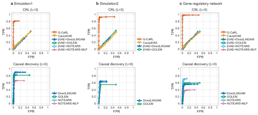
Figure 6: Illustration of the effect of the threshold for each method on Simulation 1 (a), Simulation 2 (b), and the gene regulatory network recovery task (c). The upper panels show the results with unknown observational mixings (CRL), and lower panels show the results when we applied the causal discovery frameworks directly to the latent variables (causal discovery). For each panel, ROC curve shows false positive rate (FPR) and true positive rate (TPR) with varying level of threshold, from 0% to 100% with interval of 5%, for each method. The values are the averages of 10 runs for each threshold. This result shows that G-CaRL was not so sensitive to the selection of the threshold values.

For evaluations of the estimated causal structures $\tilde{\mathbf{\bm{L}}}^{mm^{\prime}}=({\tilde{\lambda}}_{ab}^{mm^{\prime}})=(w_{1ab}^{mm^{\prime}}|w_{2ab}^{mm^{\prime}}|)$ (see Supplementary Fig. 7a for some examples), we at first converted them into binary directed (not necessarily DAG) adjacency matrices by the following procedure: we determined the causal direction on every pairs $(a,b)\in{{\mathcal{V}}_{\mathcal{S}}^{m}}\times{{\mathcal{V}}_{\mathcal{S}}^{m^{\prime}}}$ by comparing the absolute values of ${\tilde{\lambda}}_{ab}^{mm^{\prime}}$ and ${\tilde{\lambda}}_{ba}^{m^{\prime}m}$; direction is $s_{a}^{m}\rightarrow s_{b}^{m^{\prime}}$ if $|{\tilde{\lambda}}_{ab}^{mm^{\prime}}|>|{\tilde{\lambda}}_{ba}^{m^{\prime}m}|$, and vice versa. We then removed edges whose absolute weights were less than a specific ratio (35% for Simulation 1) of the maximum absolute values of both $\tilde{\mathbf{\bm{L}}}^{mm^{\prime}}$ and $\tilde{\mathbf{\bm{L}}}^{m^{\prime}m}$ for each group-pair $(m,m^{\prime})$. If both $|{\tilde{\lambda}}_{ab}^{mm^{\prime}}|$ and $|{\tilde{\lambda}}_{ba}^{m^{\prime}m}|$ are under the threshold, $s_{a}^{m}$ and $s_{b}^{m^{\prime}}$ are considered to have no direct causal relation. The obtained adjacency matrices were then compared with the (binarized) true causal structure $(\lambda_{ab}^{mm^{\prime}})$, and evaluated by F1-score ($=$ 2 $\cdot$ precision $\cdot$ recall / (precision $+$ recall)) and Structural Hamming Distance (SHD) normalized by the number of variables $D_{\mathcal{S}}$. This kind of hard thresholding is known to be effective to reduce the number of false discoveries (Zheng et al., 2018), and seems to be especially important for methods like G-CaRL which do not explicitly impose sparseness or DAG structure constraints for the estimation. The threshold-ratio was determined separately for each experiment (simulation 1 and 2, and gene regulatory network recovery), but it was not changed across the parameter settings or runs within each experiment. Our preliminary analyses showed that the G-CaRL framework was not so sensitive to the selection of the threshold values, which can be seen from the ROC curves with varying threshold (Supplementary Fig. 6). Although G-CaRL is supposed to have indeterminacy of the causal graphs with its group-pair-wise matrix-transposes (Theorem 3), we solved that indeterminacy by giving some level of constraints to the function $\psi$ (Eq. 75), where the function cannot be fitted into the opposite direction by its design. Therefore we directly used $\tilde{\mathbf{\bm{L}}}^{mm^{\prime}}$ as the final guess of $\mathbf{\bm{L}}^{mm^{\prime}}$ for each group-pair $(m,m^{\prime})$ without considering the possible matrix transpose. For solving the possible permutation of variables, we used the same permutations $\mathbf{\bm{\sigma}}^{m}$ and $\mathbf{\bm{\sigma}}^{m^{\prime}}$ estimated based on the latent variables above. We only evaluated the inter-group causal connections, since only those are identifiable in our model (Theorem 3).

Baselines

The baselines only include unsupervised frameworks with instantaneous causal interactions, since our experimental setting does not include supervision, intervention, nor temporal causality. Specifically, we used CausalVAE (Yang et al., 2021) in unsupervised setting, and the causal discovery frameworks DirectLiNGAM (Shimizu et al., 2011), NOTEARS (Zheng et al., 2018), NOTEARS-MLP (Zheng et al., 2020), GOLEM (Ng et al., 2020), PC (Spirtes and Glymour, 1991), CAM (Bühlmann et al., 2014), and CCD (Lacerda et al., 2008) (See Supplementary Material J). We cannot apply Sturma et al. (2023) since the groups have no overlap in our setting. Briefly, CausalVAE is a CRL framework, assuming linear DAG on the latent space, and the others are causal discovery frameworks. DirectLiNGAM, NOTEARS, and GOLEM are specialized at linear DAGs, CAM and NOTEARS-MLP are for nonlinear DAGs, and CCD assumes existence of directed cycles. We used publicly available implementations of them. We do not consider frameworks based on temporal causality, such as Lachapelle et al. (2022); Lippe et al. (2022); Yao et al. (2022b, a), since the samples are generated independently, with only instantaneous causality in this experiment. Note that we cannot apply many of the existing CRL frameworks designed for instantaneous causal models (e.g., Shen et al. (2022)) since they usually require supervision or interventions, which are not available in this experiment. Although CausalVAE originally requires supervision of the latent variables for the identifiability unlike our framework, we used its unsupervised setting (CausalVAE-unsup in Yang et al. (2021)), which is a reduced version of CausalVAE whose structure is the same as CausalVAE except that the Mask Layer and the supervision conditional prior were removed. For a fair comparison, we used the same architecture (group-wise disentanglement) for the encoders and the decoders of CausalVAE as in the feature extractors ${\mathbf{\bm{h}}}^{m}$ of G-CaRL.

For the baselines which do not perform representation learning by themselves (other than CausalVAE), we first applied $\beta$-VAE (Higgins et al., 2017) to achieve some level of disentanglement, although this may have little theoretical justification (we cannot use identifiable-VAE (Khemakhem et al., 2020a) since it requires weak supervision). The $\beta$-VAE has an adjustable parameter $\beta$ controlling the strength of the regularization of the latent variable distributions. We used the setting of $\beta=1$, which actually corresponds to the original-VAE (Kingma and Welling, 2014), since it gives the best estimation performance of the latent variables. For a fair comparison, we used the same architecture (group-wise disentanglement) for the encoders and the decoders of $\beta$-VAE as in the feature extractors ${\mathbf{\bm{h}}}^{m}$ of G-CaRL, similarly to CausalVAE mentioned above.

For the frameworks which output weighted adjacency matrices (CausalVAE, DirectLiNGAM, NOTEARS-linear, NOTEARS-MLP, and GOLEM), we used the same evaluation criteria to that of G-CaRL (causal direction determination, thresholding, and variable assignments). The threshold was determined separately for each method, so as to maximize the F1-score (see Supplementary Fig. 6 for the effect of the varying threshold). Although some baselines have a function to adjust the threshold so as to make the estimated graphs DAG, we instead applied the same thresholding method to ours, without constraining the acyclicity on the final graph. The other frameworks which output a binarized adjacency matrix, we directly compared them with the binarized true adjacency matrices, after variable assignments. Since some of them output graphs possibly with some bi-directional (or undetermined) edges, we gave the true directions to them favorably.

We also evaluated the causal discovery performances of the causal discovery baselines (other than CausalVAE), by applying them directly to the latent variables. In this case, we applied them after standardizing the latent variables (zero-mean and unit-variance for each variable), as suggested by (Reisach et al., 2021).

Appendix H Implementation Detail for Simulation 2

We give here more detail on the data generation and training in Simulation 2 (Section 7.2). Evaluation methods are the same to those in Simulation 1 (see Supplementary Material G), though we excluded NOTEARS and NOTEARS-MLP from the baselines because they did not give reasonable estimations, possibly due to the presence of causal cycles.

Data Generation

We generated artificial data in a similar manner to Simulation 1, though the causal graphs were designed to be much more complex, due to the presence of directed cycles and latent confounders. Basically, we firstly generated latent variables with twice of the target size of variables with possible cycles, and then simply masked half of them as unobservable variables (latent confounders) alternately for each group; there are 10 observable (non-confounder) variables and 10 latent confounders for each group $m$ (${d_{\mathcal{S}}^{m}}=10,D=30$ for observable variables).

The whole causal graph (including latent confounders) was generated separately for each group-pair as in Simulation 1, but here without considering the causal order. The intra-group sub-graphs $\mathbf{\bm{L}}^{mm}$ was generated randomly so that each variable $s_{a}^{m}$ has one other randomly selected variable $s_{a^{\prime}}^{m}$, $a^{\prime}\neq a$, in the same group as a parent. The inter-group sub-graphs $\mathbf{\bm{L}}^{mm^{\prime}}$ were generated randomly for each group-pair $(m,m^{\prime})$ so that each variable $s_{a}^{m}$ on a group $m$ has two children on other groups $m^{\prime}$, and conversely, each variable $s_{b}^{m^{\prime}}$ on a group $m^{\prime}$ has (almost) two parents on the group $m$. And similarly for the opposite direction $\mathbf{\bm{L}}^{m^{\prime}m}$. At this point, each variable is supposed to have $2M-1$ causal parents (including the latent confounders). The non-zero values of $\mathbf{\bm{L}}$ were randomly drawn from $[0.9,1]$.

The latent variables were then sampled based on the following conditional distribution for each variable $s_{a}^{m}$ at $n$-th sample:

$$s_{a}^{m(n)}\sim\exp\left(\sum_{m^{\prime}\neq m}\sum_{b\in{{\mathcal{V}}_{\mathcal{S}}^{m^{\prime}}}}-\frac{\lambda_{ba}^{m^{\prime}m}}{|\text{pa}(s_{a}^{m})|}\left(s_{b}^{m^{\prime}(n)}+|\text{pa}(s_{a}^{m})|\text{Relu}(s_{a}^{m(n)})\right)^{2}\right),$$ (76)

where $\text{pa}(s_{a}^{m})$ is the set of parents (including latent confounders) of variable $s_{a}^{m}$, deduced from the adjacency matrix, $|\text{pa}(s_{a}^{m})|$ is the number of parents, and $\text{Relu}(x)=\max(0,x)$ is a rectified linear unit. This indicates that the activity $s_{a}^{m(n)}$ is randomly generated through a Gaussian distribution with a standard deviation modulated by the inverse of root of summation of $\lambda_{ba}^{m^{\prime}m}$, and its average is negatively biased by the positive-, but not by negative-, activities of its parents (nonlinear inhibitory connection). The non-parental variables do not directly influence $s_{a}^{m}$ because the corresponding coefficients $\lambda_{ba}^{m^{\prime}m}$ are zeros as mentioned above. The inverse-scaling of $\lambda_{ba}^{m^{\prime}m}$ by $|\text{pa}(s_{a}^{m})|$ was used so that the (conditional) standard deviations of variables were approximately the same regardless of the number of parents. This sampling distribution indicates that the function $\phi$ in Eq. 8 is given by, with a simple calculation,

$$\phi(x,y)=y\text{Relu}(x).$$ (77)

Since this causal graph can have a directed cycle, we generated the data realizations based on Gibbs sampling.

After generating the latent variables, we masked half of the variables as latent confounders alternately. Since each variable needs to be causally related to at least one of the variables on some other group (Assumption A1), we generated the causal graph under a constraint that each variable $s_{a}^{m}$ has one observable child and one observable parent on all of the other groups $m^{\prime}\neq m$ after the masking, in the graph generation above.

We used MLPs for the observation models ${\mathbf{\bm{f}}}^{m}:\mathbb{R}^{{d_{\mathcal{S}}^{m}}}\rightarrow\mathbb{R}^{{d_{\mathcal{X}}^{m}}}$, as in Simulation 1.

The number of groups ($M$) was 3, the number of the observable variables was 10 for all groups (i.e., ${d_{\mathcal{S}}^{m}}={d_{\mathcal{X}}^{m}}=d^{m}=10$; the number of variables $D_{\mathcal{S}}$ was $30$ in total, and the number of latent confounds was also 30), The number of data points $n$ was $2^{20}$, and the complexity (the number of layers) of the observational mixing model $L$ was 3. We also evaluated the performances with changing those parameters to see how they affect the estimation performances (Supplementary Fig. 5).

Training (G-CaRL)

We train the nonlinear regression function in Eq. 6 with the observed data by G-CaRL. The model is basically the same as that used in Simulation 1, except for the regression function. The function $\psi:\mathbb{R}^{2}\rightarrow\mathbb{R}$ in the regression function (Eq. 6) was parameterized by

$$\psi(x,y)=y\max(a_{1}^{mm^{\prime}}(x-b_{1}^{mm^{\prime}}),a_{2}^{mm^{\prime}}(x-b_{2}^{mm^{\prime}}))$$ (78)

with some scalar parameters $a_{1}^{mm^{\prime}},b_{1}^{mm^{\prime}},a_{2}^{mm^{\prime}}$ and $b_{2}^{mm^{\prime}}$. This is based on the idea of maxout unit, and has enough degree of freedom to represent the causal effect function $\phi$ (Eq. 77). The intra-group functions $\bar{\psi}^{m}$ were parameterized by MLP. The weight parameters $w_{ab}^{mm^{\prime}}$ in the regression function (Eq. 6) are supposed to give the estimation of the causal structure $({\tilde{\lambda}}_{ab}^{mm^{\prime}})$ after training (Theorem 3; see Supplementary Fig. 7b for some examples).

Appendix I Implementation Detail for Recovery of Gene Regulatory Network

We used synthetic single-cell gene expression data generated by SERGIO (Dibaeinia and Sinha, 2020), where each gene expression is governed by a stochastic differential equation (SDE) derived from a chemical Langevin equation, with activating or repressing causal interactions with the other genes. The gene expression data generated by SERGIO were shown to be statistically comparable to real experimental data (Dibaeinia and Sinha, 2020). We used the same parameters for the differential equations as in (Dibaeinia and Sinha, 2020), but changed the hill coefficient from 2 to 6 to make the causal relations more nonlinear.

The causal graph was designed to be a DAG (as required of SERGIO) similarly to Simulation 1, but with latent confounders similarly to Simulation 2 (Supplementary Fig. 7c shows examples). More specifically, the intra-group sub-graphs $\mathbf{\bm{L}}^{mm}$ was generated randomly in same way used in Simulation 1, while the inter-group sub-graphs $\mathbf{\bm{L}}^{mm^{\prime}}$ were generated randomly for each group-pair $(m,m^{\prime})$ in the same way used in Simulation 2, but only for the group pairs $m<m^{\prime}$. To make almost all genes have children on some other group, we designated the last gene of each group $m<M$ as the leaves (have no children), and connected genes on the last group (group-$M$) to those genes as parents. The number of variables (genes) including the latent confounders was fixed to 60, we then masked half of them as the latent confounders, and divided them into 3 groups (i.e., $M=3$, and ${d_{\mathcal{S}}^{m}}=10,D=30$ for non-latent-confounder variables). The maximum contributions (weights of edges) from parental genes to target genes were set to 0.25 for all edges. We set half of the parents as activating, and the others as repressing for each gene. See Supplementary Fig. 7c for some example. The genes (variables) which do not have any parents were assigned as master regulators (MRs), and controlled by basal production rates, randomly selected from $[0.25,0.75]$. We fixed the number of samples to $2^{18}$.

For the observation model ${\mathbf{\bm{f}}}:\mathbb{R}^{{d_{\mathcal{S}}^{m}}}\rightarrow\mathbb{R}^{{d_{\mathcal{X}}^{m}}}$, we used a multilayer perceptron (MLP) with $L$ layers (excluding the input layer) similarly to Simulations 1 and 2 because there is no known realistic settings of the observational mixings in this kind of gene expression data, to the best of our knowledge. The complexity (the number of layers) of the observational mixing model $L$ was fixed 3, similarly to Simulations 1 and 2.

The function $\psi:\mathbb{R}^{2}\rightarrow\mathbb{R}$ in the regression function (Eq. 6) was parameterized as

$$\psi(x,y)=y\sum_{k=1}^{K}a_{k}\tanh(b_{k}x+c_{k}),$$ (79)

where $K=5$ is a model order, $a_{k}$, $b_{k}$, and $c_{k}$ are trainable scalar parameters. The weight parameters $w_{ab}^{mm^{\prime}}$ in the regression function (Eq. 6) are supposed to give the estimation of the causal structure $({\tilde{\lambda}}_{ab}^{mm^{\prime}})$ after training (Theorem 3; see Supplementary Fig. 7c for some examples).

Appendix J Details of Baselines

CausalVAE

CausalVAE (Yang et al., 2021) is a CRL framework based on VAE. The model is composed of an encoder and a decoder, as in vanilla VAE, while it also includes Causal Layer to represent the causal relations of the latent variables. More specifically, the input signal passes through an encoder to obtain independent exogenous factors, which are passed through a Causal Layer to generate causal representation, and then taken by the decoder to reconstruct the original input. Assumptions of linear directed acyclic causal graphs and (weak) supervision on the latent variables give the identifiability of the model up to some indeterminacy. We especially used its unsupervised setting (CausalVAE-unsup, (Yang et al., 2021)) as a baseline.

$\beta$-VAE

$\beta$-VAE (Higgins et al., 2017) is an extension of VAE (Kingma and Welling, 2014); the model architecture is the same as vanilla-VAE, while it incorporates additional regularization parameter $\beta$ for adjusting the strength of KL-divergence regularization controlling the discrepancy between the encoded latent variable distributions and their models (Gaussian). When $\beta=1$, $\beta$-VAE simply leads to the vanilla-VAE.

DirectLiNGAM

DirectLiNGAM (Shimizu et al., 2011) assumes SEMs with linear DAG and non-Gaussian errors. In the first step, DirectLiNGAM finds the causal order of variables by iteratively finding a root variable by performing regression and independence testing for each pair of variables, extracting one which is exogenous to the others, and then removing the effect of the root variable from the other ones. DirectLiNGAM then eliminates unnecessary edges using AdaptiveLasso (Zou, 2006), and outputs a weighted adjacency matrix.

NOTEARS

NOTEARS (Zheng et al., 2018) assumes linear SEMs of DAG. It estimates a weighted adjacency matrix by minimizing a least-squares loss in scoring DAGs with regularization terms imposing sparseness and DAG-ness of the adjacency matrix. Since NOTEARS formulates the structure learning problem as a continuous optimization problem over real matrices, it can effectively avoid the traditional combinatorial optimization problem (NP-hard) of learning DAGs. We used the default parameters.

NOTEARS-MLP

NOTEARS-MLP (Zheng et al., 2020) is an extension of NOTEARS (Zheng et al., 2018) to general nonparametric DAG models. NOTEARS-MLP models variable-wise nonlinear causal functions by MLPs, which are learned based on continuous optimization problem with regularizations for the sparseness of the MLP parameters and for DAG-ness of the causal functions. We used the default parameters.

GOLEM

GOLEM (Ng et al., 2020) is an efficient version of NOTEARS (Zheng et al., 2018), which can reduce number of optimization iterations. GOLEM assumes linear DAGs, and performs multivariate Gaussian maximum likelihood estimation (MLE) with a soft version of the differentiable acyclicity constraint proposed in (Zheng et al., 2018). There are two proposed models; equal(EV) or unequal (NV) noise variances. We used EV here since the estimation performances were better than NV. We used the hyper-parameters used in (Ng et al., 2020).

PC

PC algorithm (Spirtes and Glymour, 1991) is a constraint-based method. PC algorithm firstly constructs an undirected graph by removing edges from a fully connected graph based on independence and conditional independence tests. It then constructs a DAG by directing the edges based on the information of separation sets and with some additional assumptions (no new v-structures and directed cycles).

CAM

Causal additive model (CAM) (Bühlmann et al., 2014) assumes SEMs specified by DAG and additive Gaussian errors, which is an extension of linear SEMs by allowing for variable-wise scalar nonlinear functions (Collorary 31 in (Peters et al., 2014)). CAM at first estimates the causal order of variables based a greedy search algorithm so as to maximize the likelihood, then non-relevant edges were removed (pruning) by a sparse regression technique implemented based on significance testing of covariates.

CCD

Cyclic causal discovery algorithm (CCD) (Lacerda et al., 2008) assumes that the data are causally sufficient (no latent variables), while possibly includes directed cycles. CCD extracts cyclic models using conditional independence tests, as with PC (Spirtes and Glymour, 1991). The output of CCD algorithm is a cyclic partial ancestral graph (PAG), which is a graphical object that represents a set of causal Bayesian networks that cannot be distinguished by the algorithm.

References

- Acosta et al. (2022) J. N. Acosta, G. J. Falcone, P. Rajpurkar, and E. J. Topol. Multimodal biomedical ai. Nature Medicine, 28(9):1773–1784, 2022.
- Ahuja et al. (2022a) K. Ahuja, J. S Hartford, and Y. Bengio. Weakly supervised representation learning with sparse perturbations. In Advances in Neural Information Processing Systems, volume 35, pages 15516–15528, 2022a.
- Ahuja et al. (2022b) K. Ahuja, Y. Wang, D. Mahajan, and Y. Bengio. Interventional causal representation learning. In NeurIPS 2022 Workshop on Neuro Causal and Symbolic AI (nCSI), 2022b.
- Andersson et al. (1997) S. A. Andersson, D. Madigan, and M. D. Perlman. A characterization of Markov equivalence classes for acyclic digraphs. The Annals of Statistics, 25(2):505–541, 1997.
- Bengio et al. (2013) Y. Bengio, A. Courville, and P. Vincent. Representation learning: A review and new perspectives. IEEE Transactions on Pattern Analysis and Machine Intelligence, 35(8):1798–1828, 2013.
- Bollen (1989) K. A. Bollen. Structural Equations with Latent Variables. John Wiley & Sons, 1989.
- Brehmer et al. (2022) J. Brehmer, P. de Haan, P. Lippe, and T. S Cohen. Weakly supervised causal representation learning. In Advances in Neural Information Processing Systems, volume 35, pages 38319–38331, 2022.
- Bühlmann et al. (2014) P. Bühlmann, J. Peters, and J. Ernest. CAM: Causal additive models, high-dimensional order search and penalized regression. The Annals of Statistics, 42(6):2526 – 2556, 2014.
- Burkhardt et al. (2022) D. Burkhardt, M. Luecken, A. Benz, P. Holderrieth, J. Bloom, C. Lance, A. Chow, and R. Holbrook. Open problems - multimodal single-cell integration. Kaggle, 2022.
- Chen et al. (2018) R. T. Q. Chen, X. Li, R. B Grosse, and D. K Duvenaud. Isolating sources of disentanglement in variational autoencoders. In Advances in Neural Information Processing Systems, volume 31, 2018.
- Choi et al. (2020) J. Choi, R. Chapkin, and Y. Ni. Bayesian causal structural learning with zero-inflated Poisson bayesian networks. In Advances in Neural Information Processing Systems, volume 33, pages 5887–5897, 2020.
- Dibaeinia and Sinha (2020) P. Dibaeinia and S. Sinha. SERGIO: A single-cell expression simulator guided by gene regulatory networks. Cell Systems, 11(3):252–271.e11, 2020.
- Geiger and Heckerman (1994) D. Geiger and D. Heckerman. Learning Gaussian networks. In Proceedings of the Tenth international conference on Uncertainty in artificial intelligence, pages 235–243, 1994.
- Gong et al. (2015) M. Gong, K. Zhang, B. Schoelkopf, D. Tao, and P. Geiger. Discovering temporal causal relations from subsampled data. In Proceedings of the 32nd International Conference on Machine Learning, pages 1898–1906, 2015.
- Gresele et al. (2020) L. Gresele, P. K. Rubenstein, A. Mehrjou, F. Locatello, and B. Schölkopf. The incomplete Rosetta Stone problem: Identifiability results for multi-view nonlinear ICA. In Proceedings of The 35th Uncertainty in Artificial Intelligence Conference, volume 115, pages 217–227, 2020.
- Gresele et al. (2021) L. Gresele, J. Von Kügelgen, V. Stimper, B. Schölkopf, and M. Besserve. Independent mechanism analysis, a new concept? In Advances in Neural Information Processing Systems, 2021.
- Gutmann and Hyvärinen (2012) M. U. Gutmann and A. Hyvärinen. Noise-contrastive estimation of unnormalized statistical models, with applications to natural image statistics. Journal of Machine Learning Research, 13(11):307–361, 2012.
- Hälvä and Hyvärinen (2020) H. Hälvä and A. Hyvärinen. Hidden Markov nonlinear ICA: Unsupervised learning from nonstationary time series. In Proceedings of the 36th Conference on Uncertainty in Artificial Intelligence (UAI), volume 124, pages 939–948, 2020.
- Hälvä et al. (2021) H. Hälvä, S. Le Corff, L. Lehéricy, J. So, Y. Zhu, E. Gassiat, and A. Hyvarinen. Disentangling identifiable features from noisy data with structured nonlinear ica. In Advances in Neural Information Processing Systems, volume 34, pages 1624–1633, 2021.
- Hastie et al. (2001) T. Hastie, R Tibshirani, and J. Friedman. The Elements of Statistical Learning. Springer, New York, NY, 2001.
- Hebart et al. (2023) M. N Hebart, O. Contier, L. Teichmann, A. H Rockter, C. Y Zheng, A. Kidder, A. Corriveau, M. Vaziri-Pashkam, and C. I Baker. Things-data, a multimodal collection of large-scale datasets for investigating object representations in human brain and behavior. eLife, 12:e82580, 2023.
- Higgins et al. (2017) I. Higgins, L. Matthey, A. Pal, C. Burgess, X. Glorot, M. Botvinick, S. Mohamed, and A. Lerchner. -vae: Learning basic visual concepts with a constrained variational framework. In International Conference on Learning Representations, 2017.
- Horan et al. (2021) D. Horan, E. Richardson, and Y. Weiss. When is unsupervised disentanglement possible? In Advances in Neural Information Processing Systems, volume 34, pages 5150–5161, 2021.
- Hornik et al. (1989) K. Hornik, M. Stinchcombe, and H. White. Multilayer feedforward networks are universal approximators. Neural Networks, 2(5):359 – 366, 1989.
- Hoyer et al. (2008a) P. O. Hoyer, D. Janzing, J. Mooij, J. Peters, and B. Schölkopf. Nonlinear causal discovery with additive noise models. In Proceedings of the 21st International Conference on Neural Information Processing Systems, pages 689–696, 2008a.
- Hoyer et al. (2008b) P. O. Hoyer, S. Shimizu, A. J. Kerminen, and M. Palviainen. Estimation of causal effects using linear non-Gaussian causal models with hidden variables. International Journal of Approximate Reasoning, 49(2):362–378, 2008b.
- Hyvärinen and Morioka (2016) A. Hyvärinen and H. Morioka. Unsupervised feature extraction by time-contrastive learning and nonlinear ICA. In Advances in Neural Information Processing Systems (NIPS) 29, pages 3765–3773. 2016.
- Hyvarinen and Morioka (2017) A. Hyvarinen and H. Morioka. Nonlinear ICA of temporally dependent stationary sources. In AISTATS, pages 460–469, 2017.
- Hyvärinen and Pajunen (1999) A. Hyvärinen and P. Pajunen. Nonlinear independent component analysis: Existence and uniqueness results. Neural Netw., 12(3):429 – 439, 1999.
- Hyvärinen and Smith (2013) A. Hyvärinen and S. M. Smith. Pairwise likelihood ratios for estimation of non-Gaussian structural equation models. Journal of Machine Learning Research, 14(1):111–152, 2013.
- Hyvärinen et al. (2010) A. Hyvärinen, K. Zhang, S. Shimizu, and P. O. Hoyer. Estimation of a structural vector autoregression model using non-Gaussianity. Journal of Machine Learning Research, 11(56):1709–1731, 2010.
- Hyvarinen et al. (2019) A. Hyvarinen, H. Sasaki, and R. Turner. Nonlinear ICA using auxiliary variables and generalized contrastive learning. In AISTATS, pages 859–868, 2019.
- Khemakhem et al. (2020a) I. Khemakhem, D. P. Kingma, R. P. Monti, and A. Hyvärinen. Variational autoencoders and nonlinear ICA: A unifying framework. In AISTATS, 2020a.
- Khemakhem et al. (2020b) I. Khemakhem, R. Monti, D. Kingma, and A. Hyvarinen. Ice-beem: Identifiable conditional energy-based deep models based on nonlinear ica. In Advances in Neural Information Processing Systems, volume 33, pages 12768–12778, 2020b.
- Kim and Mnih (2018) H. Kim and A. Mnih. Disentangling by factorising. In Proceedings of the 35th International Conference on Machine Learning, volume 80, pages 2649–2658, 2018.
- Kingma and Welling (2014) D. P Kingma and M. Welling. Auto-encoding variational bayes. In ICLR, 2014.
- Kivva et al. (2021) B. Kivva, G. Rajendran, P. Ravikumar, and B. Aragam. Learning latent causal graphs via mixture oracles. In Advances in Neural Information Processing Systems, volume 34, pages 18087–18101, 2021.
- Klindt et al. (2021) D. A. Klindt, L. Schott, Y. Sharma, I. Ustyuzhaninov, W. Brendel, M. Bethge, and D. Paiton. Towards nonlinear disentanglement in natural data with temporal sparse coding. In International Conference on Learning Representations, 2021.
- Lacerda et al. (2008) G. Lacerda, P. Spirtes, J. Ramsey, and P. O. Hoyer. Discovering cyclic causal models by independent components analysis. In Proceedings of the Twenty-Fourth Conference on Uncertainty in Artificial Intelligence, pages 366–374, 2008.
- Lachapelle et al. (2022) S. Lachapelle, P. Rodriguez, Y. Sharma, K. E Everett, R. LE PRIOL, A. Lacoste, and S. Lacoste-Julien. Disentanglement via mechanism sparsity regularization: A new principle for nonlinear ICA. In Proceedings of the First Conference on Causal Learning and Reasoning, volume 177, pages 428–484, 2022.
- Leeb et al. (2022) F. Leeb, G. Lanzillotta, Y. Annadani, M. Besserve, S. Bauer, and B. Schölkopf. Structure by architecture: Disentangled representations without regularization. In UAI 2022 Workshop on Causal Representation Learning, 2022.
- Li et al. (2020) Y. Li, A. Torralba, A. Anandkumar, D. Fox, and A. Garg. Causal discovery in physical systems from videos. In Advances in Neural Information Processing Systems, volume 33, pages 9180–9192, 2020.
- Lippe et al. (2022) P. Lippe, S. Magliacane, S. Löwe, Y. M Asano, T. Cohen, and E. Gavves. CITRIS: Causal identifiability from temporal intervened sequences. In ICLR2022 Workshop on the Elements of Reasoning: Objects, Structure and Causality, 2022.
- Lippe et al. (2023) P. Lippe, S. Magliacane, S. Löwe, Y. M Asano, T. Cohen, and E. Gavves. Causal representation learning for instantaneous and temporal effects in interactive systems. In The Eleventh International Conference on Learning Representations, 2023.
- Locatello et al. (2019) F. Locatello, S. Bauer, M. Lucic, G. Raetsch, S. Gelly, B. Schölkopf, and O. Bachem. Challenging common assumptions in the unsupervised learning of disentangled representations. In Proceedings of the 36th International Conference on Machine Learning, volume 97, pages 4114–4124, 2019.
- Locatello et al. (2020) F. Locatello, B. Poole, G. Raetsch, B. Schölkopf, O. Bachem, and M. Tschannen. Weakly-supervised disentanglement without compromises. In Proceedings of the 37th International Conference on Machine Learning, volume 119, pages 6348–6359, 2020.
- Longman et al. (2018) R. J. Longman, T. W. Giambelluca, M. A. Nullet, A. G. Frazier, K. Kodama, S. D. Crausbay, P. D. Krushelnycky, S. Cordell, M. P. Clark, A. J. Newman, and J. R. Arnold. Compilation of climate data from heterogeneous networks across the Hawaiian islands. Scientific Data, 5(1):180012, 2018.
- Maeda and Shimizu (2020) T. N. Maeda and S. Shimizu. RCD: Repetitive causal discovery of linear non-Gaussian acyclic models with latent confounders. In Proceedings of the Twenty Third International Conference on Artificial Intelligence and Statistics, pages 735–745, 2020.
- Monti et al. (2020) R. P. Monti, K. Zhang, and A. Hyvärinen. Causal discovery with general non-linear relationships using non-linear ICA. In Proceedings of The 35th Uncertainty in Artificial Intelligence Conference, volume 115, pages 186–195, 2020.