A posteriori error estimates for nonconforming discretizations of singularly perturbed biharmonic operators

Abstract.

For the pure biharmonic equation and a biharmonic singular perturbation problem, a residual-based error estimator is introduced which applies to many existing nonconforming finite elements. The error estimator involves the local best-approximation error of the finite element function by piecewise polynomial functions of the degree determining the expected approximation order, which need not coincide with the maximal polynomial degree of the element, for example if bubble functions are used. The error estimator is shown to be reliable and locally efficient up to this polynomial best-approximation error and oscillations of the right-hand side.

1. Introduction

Given an open and bounded polytopal Lipschitz domain $\Omega\subseteq\mathbb{R}^{d}$ in dimension $d\in\{2,3\}$, we consider the following model problem of the biharmonic type. Given a parameter $\varepsilon\in(0,1]$ and $\alpha\in\{0,1\}$ and a right-hand side function $f$, we seek the solution $u$ to

(1.1) $$\begin{cases}\varepsilon^{2}\triangle^{2}u-\alpha\triangle u=f\quad&\text{in }\Omega,\\ u=\frac{\partial u}{\partial n}=0\quad&\text{on }\partial\Omega.\end{cases}$$

Here, $n$ denotes the outer unit normal to $\partial\Omega$. We focus on two choices of parameters. For $\varepsilon=1$ and $\alpha=0$, we obtain the biharmonic equation

$$\triangle^{2}u=f\quad\text{in }\Omega$$

subject to clamped boundary conditions. For the choice of a possibly small positive parameter $\varepsilon$ and $\alpha=1$, we obtain the singularly perturbed fourth-order problem

$$\varepsilon^{2}\triangle^{2}u-\triangle u=f\quad\text{in }\Omega$$

with clamped boundary conditions. These are the two relevant scenarios because for $\alpha=0$, the problem can always be reduced to the biharmonic equation after scaling of the right-hand side. If $\alpha=1$, the problem is singularly perturbed and the solution $u_{0}$ to

$$-\triangle u_{0}=f\quad\text{in }\Omega\quad\text{and}\quad u_{0}=0\quad\text{on }\partial\Omega$$

corresponds to the formal limit $\varepsilon=0$.

It is known that some nonconforming finite element methods are convergent for the pure biharmonic equation but not for Poisson’s equation and therefore perform poorly for the singularly perturbed problem (1.1). For example, in [22] the failure of the Morley element was rigorously shown and a $C^{0}$ conforming alternative similar to the Morley element was proposed.

For the biharmonic equation, a posteriori error estimators were established for the Morley element [1] and for some low-order rectangular elements [4]. Under additional regularity assumptions, an a posteriori error estimate for the Specht element was derived in [26]. Beyond these references, there are no a posteriori error estimates available for nonconforming discretizations of (1.1). The difficulty typically encountered in the a posteriori error analysis of nonconforming finite element methods for the biharmonic equation is that they usually do not contain a suitable conforming subspace. In the reliability proof, the error can therefore not be approximated by a conforming finite element function that is a valid test function for the discrete problem. When the error is interpolated by a nonconforming function, care has to be taken that non-residual face terms resulting from an integration by parts have suitable orthogonality properties. Such properties fail to hold for most of the existing methods because the maximal polynomial degree (henceforth denoted by $L$) of the shape functions is higher than the degree of weak continuity across the elements in the triangulation. Such high-degree polynomial are, however, often relevant to the well-posedness (stability) of the method (a set of shape functions for which the degrees of freedom are linear independent is required), but irrelevant, in the generic case, to the approximation order prescribed by the maximal degree $\ell$ of polynomials that are fully included in the local shape function space. The technique we propose in this work is therefore to include a new term in the residual-based a posteriori error estimator. For a simplex $T$ in the triangulation and the finite element solution $u_{h}$ it reads

$$\lvert\!\lvert\!\lvert u_{h}-\Pi_{\ell}u_{h}\rvert\!\rvert\!\rvert_{T}$$

for the $L^{2}$ projection $\Pi_{\ell}$ to the polynomial functions of degree not larger than $\ell$ over $T$. The precise definition of the energy seminorm $\lvert\!\lvert\!\lvert\cdot\rvert\!\rvert\!\rvert_{T}$ can be found in Section 2.3. Scaling arguments and the triangle inequality show that this term is locally efficient up to the best approximation of the exact solution $u$ by piecewise polynomials of degree $\ell$. It turns out that this approach enables a posteriori error estimates for a large class of nonconforming elements characterized by the weak continuity from Assumption 2.1 below and covers many existing methods for which no a posteriori estimates have been available before, see Table 1.

An important application of this idea is the design of a posteriori error estimators for the fourth-order singular perturbation problem. For discontinuous $H^{2}$-nonconforming elements, the weak continuity properties of the function value jump are usually weaker than those of the the gradient jump, see, e.g., [21, 18]. Consequently, such nonconforming elements tend to lose two orders of approximation when the parameter $\epsilon$ becomes small. Consequently, as mentioned above, employing the Morley element directly in this problem does not lead to convergence. One remedy proposed in [34] is to utilize a modified bilinear form with the $P_{1}$ Lagrange interpolation in the second-order term. This technique, known as the modified Morley method, can also be extended to three-dimensional cases [30]. The idea of the modified Morley element in 2D extends to other discontinuous $H^{2}$-nonconforming methods as outlined in [18]. However such methods still do not reach the full convergence rate when $\epsilon$ is small. Hence, $C^{0}$-conforming but $H^{2}$-nonconforming elements are particularly attractive for the singular perturbation problem [22, 14]. In the literature, Wang and Zhang [37] developed error estimators for some low-order nonconforming elements assuming $H^{3}$ regularity. Nevertheless, there have been no results under minimal regularity assumptions or for high-order methods or $d\geq 3$ so far. For the singularly perturbed Laplacian, parameter-robust a posteriori error estimators were derived [28]. We combine these techniques with the approach outlined above for proving a posteriori error estimates for the bi-Laplacian in the singularly perturbed case.

The remaining parts of this article are organized as follows. Section 2 provides preliminaries on the model problem and the finite element discretization. The reliability and efficiency of the error estimator are proven in Section 3. Section 4 is devoted to examples and Section 5 reports numerical experiments. For convenient reading, some technical details are listed as Appendix A and B.

Standard notation for function spaces is used throughout the article. The inner product in the Lebesgue space $L^{2}(\omega)$ with respect to $\omega\subseteq\Omega$ is denoted by $(\cdot,\cdot)_{0,\omega}$, and the $L^{2}$ norm over $\omega$ is denoted by $\|\cdot\|_{0,\omega}$. If $\omega=\Omega$, we simply write $(\cdot,\cdot)_{0}$ and $\|\cdot\|_{0}$. The second-order $L^{2}$-based Sobolev space with clamped boundary condition is denoted by $V:=H^{2}_{0}(\Omega)$. The Euclidean inner product of $x,y\in\mathbb{R}^{n}$ is denoted by $x\cdot y$. The divergence operator for matrix-valued functions is understood row-wise. The notation $a\lesssim b$ means the inequality $a\leq Cb$ up to a multiplicative constant $C$ that does not depend on the mesh-size $h$ or the parameter $\varepsilon$.

2. Preliminaries

2.1. Weak formulation of the model problem

The weak formulation of (1.1) is based on the Sobolev space $V:=H^{2}_{0}(\Omega)$. Given $f\in L^{2}(\Omega)$, it seeks $u\in V$ such that

(2.1) $$a(u,v)=(f,v)_{0}\quad\text{for all }v\in V$$

for the bilinear form

$$a(u,v)=\varepsilon^{2}(D^{2}u,D^{2}v)_{0}+\alpha(\nabla u,\nabla v)_{0}.$$

We denote the induced energy norm by $\|v\|_{a}:=a(v,v)^{1/2}$.

2.2. Discrete functions

Throughout this work, we assume an underlying regular simplicial triangulation $\mathcal{T}$ of the domain $\Omega$ from a shape-regular family. For each element $T\in\mathcal{T}$, the diameter of $T$ is denoted by $h_{T}$, and by $h$ we denote the piecewise constant mesh-size function defined by $h|_{T}=h_{T}$ for any $T\in\mathcal{T}$. The set of $(d-1)$-dimensional hyperfaces is denoted by $\mathcal{F}$. The subset of interior faces is denoted by $\mathcal{F}(\Omega)$. The diameter of a face $F$ is denoted by $h_{F}$. Any interior face $F\in\mathcal{F}(\Omega)$ is shared by two elements, which we denote by $T_{+},T_{-}\in\mathcal{T}$. If $F$ is a boundary face, $T_{+}$ is the unique element containing $F$ and we use the convention $T_{-}=\emptyset$. The interior of $T_{+}\cup T_{-}$ is denoted by $\omega_{F}$ and referred to as the face patch of $F$. To every face $F\in\mathcal{F}$ we assign a unit normal vector $n_{F}$. If $F\subset\partial\Omega$ is a boundary face, we choose $n_{F}$ to be outward-pointing with respect to $\Omega$. The set of vertices in the triangulation is denoted by $\mathcal{N}$. Given a vertex $y\in\mathcal{N}$, its vertex patch $\omega_{y}$ is the interior of the union of all elements of $\mathcal{T}$ that contain $y$; the diameter of the vertex patch is denoted by $h_{y}$. The jump and the average of a function $v$ on an interior face $F\in\mathcal{F}(\Omega)$ are defined as $[v]|_{F}:=v_{+}-v_{-}$ and $\{v\}|_{F}:=2^{-1}(v_{+}+v_{-})$. Here we set $v_{\pm}:=v|_{T_{\pm}}$. If $F\subseteq\partial\Omega$ is a boundary face, we set $[v]|_{F}=\{v\}_{F}=v|_{T_{+}}$.

The symbols $\nabla_{h}$, $\operatorname{div}_{h}$, $D^{2}_{h}$, $\triangle_{h}$ denote the $\mathcal{T}$-piecewise application of the differential operators $\nabla$, $\operatorname{div}$, $D^{2}$, $\triangle$, respectively. Given a subdomain $\omega\subseteq\bar{\Omega}$, the space of polynomial functions over $\omega$ of degree not larger than $\ell\geq 0$ is denoted by $P_{\ell}(\omega)$. The piecewise polynomial functions with respect to $\mathcal{T}$ are denoted by

$$P_{\ell}(\mathcal{T})=\{v\in L^{2}(\Omega):v|_{T}\in P_{\ell}(T)\text{ for any }T\in\mathcal{T}\}.$$

The $L^{2}(\Omega)$-orthogonal projection onto $P_{\ell}(\mathcal{T})$ is denoted by $\Pi_{\ell}$.

2.3. Finite element discretization

The finite element space $V_{h}$ is assumed to be a subspace of the piecewise polynomial functions with some given maximal degree $L$, i.e., $V_{h}\subseteq P_{L}(\mathcal{T})$. On $V+V_{h}$, we introduce the semidefinite bilinear form

$$a_{h}(u,v)=\varepsilon^{2}(D_{h}^{2}u,D_{h}^{2}v)_{0}+\alpha(\nabla_{h}u,\nabla_{h}v)_{0}$$

with seminorm $\|v\|_{a,h}:=a_{h}(v,v)^{1/2}$. We assume throughout that any element $v_{h}\in V_{h}$ satisfies the weak continuity condition

(2.2) $$\|[v_{h}]_{F}\|_{0,F}\lesssim h_{F}\|\nabla_{F}[v_{h}]_{F}\|_{0,F}\quad\text{for all }F\in\mathcal{F}$$

where $\nabla_{F}$ is the tangential gradient operator on $F$. Condition (2.2) and Assumption 2.1 below guarantee that $a_{h}$ is positive definite over $V_{h}$ such that $\|\cdot\|_{a,h}$ is a norm on $V_{h}$, see Lemma 2.2 for a proof. We further assume the existence of an operator $J_{h}:V\to V_{h}$ with the approximation and stability properties

(2.3a) $$\|h^{-2}(v-J_{h}v)\|_{0}+\|h^{-1}\nabla_{h}(v-J_{h}v)\|_{0}+\|D_{h}^{2}(v-J_{h}v)\|_{0}\lesssim\|D^{2}v\|_{0}$$

and

(2.3b) $$\|h^{-1}(v-J_{h}v)\|_{0}+\|\nabla_{h}(v-J_{h}v)\|_{0}\lesssim\|\nabla v\|_{0}$$

for all $v\in V$. Such operators, referred to as quasi-interpolation operators, are usually defined as a regularization by local averaging, see [9]. We will also use, for measurable subsets $\omega\subseteq\Omega$, the localized seminorm

$$\lvert\!\lvert\!\lvert w\rvert\!\rvert\!\rvert_{\omega}:=\left(\varepsilon^{2}\|D^{2}_{h}w\|_{0,\omega}^{2}+\alpha\|\nabla_{h}w\|_{0,\omega}^{2}\right)^{1/2}\quad\text{for any }w\in V+V_{h},$$

for which we have $\lvert\!\lvert\!\lvert w\rvert\!\rvert\!\rvert_{\Omega}=\|w\|_{a,h}$. An application of inverse inequalities shows that the $L^{2}$ projection $\Pi_{\ell}$ is quasi-optimal with respect to the seminorm $\lvert\!\lvert\!\lvert\cdot\rvert\!\rvert\!\rvert_{T,\alpha,\omega}$, i.e.,

(2.4) $$\lvert\!\lvert\!\lvert w_{L}-\Pi_{\ell}w_{L}\rvert\!\rvert\!\rvert_{T,\alpha,\omega}\lesssim\min_{v_{\ell}\in P_{\ell}(T)}\lvert\!\lvert\!\lvert w_{L}-v_{\ell}\rvert\!\rvert\!\rvert_{T,\alpha,\omega}\quad\text{for any }w_{L}\in P_{L}(T).$$

While $L$ denotes the highest polynomial degree used for the local shape functions of $V_{h}$, usually $P_{L}(T)$ will not be a subset of the local shape function space defining the underlying finite element; a typical instance of such incomplete polynomial shape function spaces is the enrichment by bubble functions. It is instead assumed that the shape function space contains $P_{\ell}(T)$ for some $\ell\leq L$. Following [18], we formulate the following consistency condition for the inter-element jumps.

Assumption 2.1.

There exists $\ell\geq 2$ such that any element $v_{h}\in V_{h}$ from the finite element space $V_{h}$ with respect to $\mathcal{T}$ satisfies, for any $F\in\mathcal{F}$,

(2.5a) $$[v_{h}]_{F}=0 \text{if }\alpha=1,$$ pointwise

(2.5b) $$\int_{F}[v_{h}]_{F}q\mathrm{d}S=0 \text{for all }q\in P_{\ell-3}(F) \text{if }\alpha=0,$$

(2.5c) $$\int_{F}[\nabla_{h}v_{h}]_{F}\cdot Q\mathrm{d}S=0\quad \text{for all }Q\in(P_{\ell-2}(F))^{d}.$$

Here, we follow the convention that $P_{-1}(F)=\{0\}$.

The finite element discretization of (2.1) seeks $u_{h}\in V_{h}$ such that

(2.6) $$a_{h}(u_{h},v_{h})=(f,v_{h})_{0}\quad\text{for all }v_{h}\in V_{h}.$$

The well-posedness of the discrete problem is a consequence of the following lemma.

Lemma 2.2.

The weak continuity (2.2) and Assumption 2.1 imply that $a_{h}$ is positive definite over $V+V_{h}$.

Proof.

Any $v\in V+V_{h}$ with $a_{h}(v,v)=0$ is piecewise affine. The combination of (2.2) and (2.5c) (recall $\ell\geq 2$) therefore shows that $v$ is globally continuous. Since by (2.5c) the gradient does not jump across the inter-element faces, $v$ is globally affine. By employing (2.2) and (2.5c) on the boundary faces, we deduce $v=0$. ∎

3. A posteriori error estimates

3.1. Preparatory identities

We use the following error decomposition [4] based on the Pythagorean identity.

Lemma 3.1.

Any $u\in V$ and $u_{h}\in V_{h}$ satisfy

$$\|u-u_{h}\|_{a,h}^{2}=\sup_{v\in V,\|v\|_{a}=1}|a_{h}(u-u_{h},v)|^{2}+\min_{v\in V}\|u_{h}-v\|_{a,h}^{2}.$$

In order to estimate the first term on the right-hand side of the foregoing error decomposition, we note some basic identities based on integration by parts.

Lemma 3.2 (integration by parts).

Let Assumption 2.1 hold. Let $u_{h}\in V_{h}$ and $w\in V+V_{h}$ be given. Then, for $\ell$ as in Assumption 2.1 and any $p_{h}\in P_{\ell}(\mathcal{T})$,

$$(D_{h}^{2}u_{h},D_{h}^{2}w)_{0}=(\triangle_{h}^{2}u_{h},w)_{0}+T_{1}+T_{2}$$

where

$$T_{1}:=\sum_{F\in\mathcal{F}(\Omega)}\left(\int_{F}[D_{h}^{2}u_{h}]_{F}n_{F}\cdot\{\nabla_{h}w\}_{F}\mathrm{d}S-\int_{F}[\operatorname{div}_{h}D_{h}^{2}u_{h}]_{F}\cdot n_{F}\{w\}_{F}\mathrm{d}S\right)$$

and

$$T_{2}:=\sum_{F\in\mathcal{F}}\left(\int_{F}\{D_{h}^{2}(u_{h}-p_{h})\}_{F}n_{F}\cdot[\nabla_{h}w]_{F}\mathrm{d}S-\int_{F}\{\operatorname{div}_{h}D_{h}^{2}(u_{h}-p_{h})\}_{F}\cdot n_{F}[w]_{F}\mathrm{d}S\right).$$

If $\alpha=1$, we have

$$(\nabla_{h}u_{h},\nabla_{h}w)_{0}=-(\triangle_{h}u_{h},w)_{0}+T_{3}$$

where

$$T_{3}:=\sum_{F\in\mathcal{F}(\Omega)}\int_{F}[\nabla_{h}u_{h}]_{F}\cdot n_{F}\{w\}_{F}\mathrm{d}S.$$

Proof.

The first identity follows from piecewise integration by parts and the properties (2.5), which guarantee that on every face $F$, the functions $[\nabla_{h}w]_{F}$ and $[w]_{F}$ are orthogonal to $\{D_{h}^{2}p_{h}\}_{F}n_{F}$ and $\{\operatorname{div}_{h}D_{h}^{2}p_{h}\}_{F}\cdot n_{F}$, respectively. The second stated identity follows from piecewise integration by parts and the property (2.5a) for $\alpha=1$. ∎

3.2. Error estimator contributions

As in [28], we define the comparison coefficient $\kappa_{T}=\min\{1,h_{T}/\varepsilon\}$ of the mesh size $h_{T}$ and $\varepsilon$. Similarly, we write $\kappa_{F}=\min\{1,h_{F}/\varepsilon\}$ and $\kappa_{y}=\min\{1,h_{y}/\varepsilon\}$ for a face $F$ or a vertex $y$. We denote

$$\mu_{0}^{2}(T):=\lvert\!\lvert\!\lvert u_{h}-\Pi_{\ell}u_{h}\rvert\!\rvert\!\rvert_{T}^{2}, \mu_{1}^{2}(T):=\kappa_{T}^{2}h_{T}^{2}\|\varepsilon^{2}\triangle_{h}^{2}u_{h}-\alpha\triangle_{h}u_{h}-f\|^{2}_{0,T},$$

$$\mu_{2}^{2}(F):=\varepsilon^{3}\kappa_{F}\|[D_{h}^{2}u_{h}]_{F}n_{F}\|_{0,F}^{2}, \mu_{3}^{2}(F):=\kappa^{2}_{F}h_{F}\|[\alpha\nabla_{h}u_{h}-\varepsilon^{2}\mathrm{div}_{h}D^{2}_{h}u_{h}]_{F}\cdot n_{F}\|^{2}_{0,F}$$

for any $T\in\mathcal{T}$ and any interior face $F\in\mathcal{F}(\Omega)$. For boundary faces $F\subseteq\partial\Omega$ we set $\mu_{2}^{2}(F)=\mu_{3}^{2}(F)=0$. We abbreviate

$$\mu_{j}(\mathcal{T}):=\sqrt{\sum_{T\in\mathcal{T}}\mu_{j}^{2}(T)},\quad\mu_{k}(\mathcal{F}):=\sqrt{\sum_{F\in\mathcal{F}}\mu_{k}^{2}(F)},\quad\text{ for }j=0,1\text{ and }k=2,3.$$

We further define, for any face $F\in\mathcal{F}$,

$$\xi^{2}(F):=\frac{\varepsilon}{\kappa_{F}}\|[\nabla_{h}u_{h}]_{F}\cdot n_{F}\|^{2}_{0,F}+\frac{1}{\varepsilon\kappa_{F}^{3}}\|[u_{h}]_{F}\|^{2}_{0,F}\;\text{and}\;\xi(\mathcal{F}):=\sqrt{\sum_{F\in\mathcal{F}}\xi^{2}(F)}.$$

3.3. Error estimator reliability

We begin by bounding the first term of the decomposition from Lemma 3.1.

Lemma 3.3 (equilibrium residual).

Let Assumption 2.1 hold. Let $u\in V$ solve (2.1) and let $u_{h}\in V_{h}$ solve (2.6). Then, for any $v\in V$ with $\|v\|_{a}=1$ we have

$$a(u-u_{h},v) \lesssim\mu_{0}(\mathcal{T})+\mu_{1}(\mathcal{T})+\mu_{2}(\mathcal{F})+\mu_{3}(\mathcal{F}).$$

Proof.

We consider the quasi-interpolation $J_{h}v\in V_{h}$ of the function $v$ satisfying (2.3) and abbreviate $w:=v-J_{h}v$. We deduce from the solution properties (2.1) and (2.6) of $u$ and $u_{h}$ that

$$a_{h}(u-u_{h},v)=(f,w)_{0}-a_{h}(u_{h},w).$$

We apply integration by parts to the second term on the right-hand side: from Lemma 3.2 with $p_{h}:=\Pi_{\ell}u_{h}$ we obtain

$$(f,w)_{0}-a_{h}(u_{h},w)=(f-\varepsilon^{2}\triangle_{h}^{2}u_{h}+\alpha\triangle_{h}u_{h},w)_{0}-\varepsilon^{2}T_{1}-\varepsilon^{2}T_{2}-\alpha T_{3}$$

with $T_{1},T_{2},T_{3}$ as in Lemma 3.2. For the first term on the right-hand side of this identity, (2.3) leads to

$$(f-\varepsilon^{2}\triangle_{h}^{2}u_{h}+\alpha\triangle_{h}u_{h},w)_{0}\lesssim\mu_{1}(\mathcal{T}).$$

The trace inequality, properties (2.3), and the bounded overlap of patches show

$$\sum_{F\in\mathcal{F}}\kappa_{F}^{-2}h_{F}^{-1}\|\{w\}_{F}\|_{0,F}^{2}\lesssim\sum_{F\in\mathcal{F}}\kappa_{F}^{-2}(h_{F}^{-2}\|w\|_{0,\omega_{F}}^{2}+\|\nabla_{h}w\|_{0,\omega_{F}}^{2})\lesssim\|v\|_{a}=1.$$

Similarly, with the multiplicative trace inequality

$$\|\{\nabla_{h}w\}_{F}\|_{0,F}\lesssim h_{F}^{-1/2}\|\nabla_{h}w\|_{0,\omega_{F}}+\|\nabla_{h}w\|_{0,\omega_{F}}^{1/2}\|D^{2}_{h}w\|_{0,\omega_{F}}^{1/2}$$

we obtain

$$\sum_{F\in\mathcal{F}}\varepsilon\kappa_{F}^{-1}\|\{\nabla w\}_{F}\|_{0,F}^{2}\lesssim\|v\|_{a}=1.$$

The Cauchy inequality and the foregoing trace estimates therefore establish

$$|\varepsilon^{2}T_{1}+\alpha T_{3}|\lesssim\mu_{2}(\mathcal{F})+\mu_{3}(\mathcal{F}).$$

Similarly, trance and inverse inequalities and (2.3) give

$$|\varepsilon^{2}T_{2}|\lesssim\mu_{0}(\mathcal{T}).$$

This concludes the proof. ∎

We proceed with estimating the second term in the error decomposition of Lemma 3.1, which refer to as the conformity residual. As in [4], we shall bound that term from above by designing a suitable conforming finite element approximation to $u_{h}$. The construction is based on averaging operators employing generalized Hsieh–Clough–Tocher (HCT) spaces, the details of which are summarized in Appendix A for convenient reading. The general design of such averaged approximations is well known, see [3, 12]. In the case of a singular perturbation, such average approximation may be required on some local sub-mesh. We use the following localization argument.

Lemma 3.4 (localization).

Given any $u_{h}\in V_{h}$, we have

$$\min_{v\in V}\|u_{h}-v\|_{a,h}^{2}$$

$$\lesssim\sum_{y\in\mathcal{N}}\min_{v_{y}\in V(\omega_{y})}\left(\frac{1}{h_{y}^{2}\kappa_{y}^{2}}\|u_{h}-v_{y}\|_{0,\omega_{y}}^{2}+\frac{1}{\kappa_{y}^{2}}\|\nabla_{h}(u_{h}-v_{y})\|_{0,\omega_{y}}^{2}+\varepsilon^{2}\|D^{2}_{h}(u_{h}-v_{y})\|_{0,\omega_{y}}^{2}\right)$$

where $V(\omega_{y})$ is the space of functions over the vertex patch $\omega_{y}$ that admit an extension to $\Omega$ that belongs to $V$.

Proof.

The proof is postponed to Appendix B. ∎

Lemma 3.5 (conformity residual).

Let Assumption 2.1 hold. For $u_{h}\in V_{h}$, we have $\min_{v\in V}\|u_{h}-v\|_{a,h}\lesssim\xi(\mathcal{F}).$

Proof.

We begin with the localization from Lemma 3.4 and consider a vertex $y\in\mathcal{N}$ with vertex patch $\omega_{y}$ of diameter $h_{y}$. We denote by $\mathcal{F}(y)$ the set faces $F\in\mathcal{F}$ with $y\in F$. We denote by $\hat{\mathcal{T}}=\hat{\mathcal{T}}(\omega_{y})$ a uniformly refined triangulation of the patch $\omega_{y}$ of mesh size

(3.1) $$\max_{\hat{T}\in\hat{\mathcal{T}}}\operatorname{diam}(\hat{T})=:\hat{h}\leq\varepsilon\lesssim\kappa_{y}^{-1}\hat{h}$$

Let $\hat{V}_{C}\subseteq V(\omega_{y})$ denote the conforming generalized HCT finite element space [6, 12, 15] whose local shape functions contain $P_{L}(\hat{T})$ for any $\hat{T}\in\hat{\mathcal{T}}$. The operator $\hat{\Pi}_{C}:V_{h}|_{\omega_{F}}\to\hat{V}_{C}$ assigns a lifted object $\hat{\Pi}_{C}u_{h}$ to $u_{h}|_{\omega_{z}}$ by setting any global degree of freedom (with respect to $\hat{V}_{C}$) as the average of the evaluation of the local node functionals applied to $u_{h}|_{\omega_{z}}$. Since the degrees of freedom of the HCT functions are point evaluations of the function and the gradient in the vertices, evaluations of the normal derivative over the faces, and evaluations inside the element, standard arguments with triangle and inverse inequalities show that

$$\hat{h}^{-4}\|u_{h}-\hat{\Pi}_{C}u_{h}\|_{0,\hat{T}}^{2}\lesssim\sum_{\begin{subarray}{c}\hat{F}\in\hat{\mathcal{F}}(\hat{T})\\ \exists F\in\mathcal{F}:\hat{F}\subseteq F\in\mathcal{F}(y)\end{subarray}}(\hat{h}^{-1}\|[\nabla_{h}u_{h}]_{\hat{F}}\cdot n_{\hat{F}}\|^{2}_{0,\hat{F}}+\hat{h}^{-3}\|[u_{h}]_{\hat{F}}\|^{2}_{0,\hat{F}})$$

for any $\hat{T}\in\hat{\mathcal{T}}$ with set of faces $\hat{\mathcal{F}}(\hat{T})$. The sum is taken over all (fine) faces of $\hat{T}$ that are included in an element of $\mathcal{F}(y)$. Since $u_{h}$ is a polynomial function in each coarse simplex, its jumps are only nontrivial along the faces $F\in\mathcal{F}(y)$. We conclude

$$\hat{h}^{-4}\|u_{h}-\hat{\Pi}_{C}u_{h}\|_{0,\omega_{y}}^{2}\lesssim\sum_{F\in\mathcal{F}(y)}(\hat{h}^{-1}\|[\nabla_{h}u_{h}]_{F}\cdot n_{F}\|^{2}_{0,F}+\hat{h}^{-3}\|[u_{h}]_{F}\|^{2}_{0,F}).$$

Using inverse estimates over $\hat{\mathcal{T}}$ and the above scaling (3.1) of $\hat{h}$, we thus obtain

$$\frac{1}{h_{y}^{2}\kappa_{y}^{2}}\|u_{h}-\hat{\Pi}_{C}u_{h}\|_{0,\omega_{y}}^{2}+\frac{1}{\kappa_{y}^{2}}\|\nabla_{h}(u_{h}-\hat{\Pi}_{C}u_{h})\|_{0,\omega_{y}}^{2}+\varepsilon^{2}\|D^{2}_{h}(u_{h}-\hat{\Pi}_{C}u_{h})\|_{0,\omega_{y}}^{2}$$

$$\qquad\lesssim\sum_{F\in\mathcal{F}(y)}\left[\frac{\varepsilon}{\kappa_{F}}\|[\nabla_{h}u_{h}]_{F}\cdot n_{F}\|^{2}_{0,F}+\frac{1}{\varepsilon\kappa_{F}^{3}}\|[u_{h}]_{F}\|^{2}_{0,F}\right]=\sum_{F\in\mathcal{F}(y)}\xi^{2}(F).$$

Inserting this upper bound in the sum on the right hand side of the displayed formula from Lemma 3.4 concludes the proof. ∎

We conclude the reliability of the error estimator

$$\eta(\mathcal{T}):=\mu_{0}(\mathcal{T})+\mu_{1}(\mathcal{T})+\mu_{2}(\mathcal{F})+\mu_{3}(\mathcal{F})+\xi(\mathcal{F}).$$

Theorem 3.6 (reliability).

Let Assumption 2.1 hold. The solutions $u\in V$ to (2.1) and $u_{h}\in V_{h}$ to (2.6) satisfy

$$\|u-u_{h}\|_{a,h}\lesssim\eta.$$

Proof.

The result follows from combining Lemma 3.3 and Lemma 3.5. ∎

3.4. Error estimator efficiency

The error estimator $\eta$ is locally efficient up to data oscillations and the best-approximation by piecewise polynomials of degree $\ell$. The proofs partly follow standard arguments [29, 28] and we only highlight some important aspects in the analysis. Given $f\in L^{2}(\Omega)$, we define its oscillations of order $\ell$ with respect to $T\in\mathcal{T}$ as

$$\operatorname{osc}^{2}(f,\ell,T)=h_{T}^{2}\kappa_{T}^{2}\|f-\Pi_{\ell}f\|^{2}_{0,T}.$$

Theorem 3.7 (local efficiency).

Let Assumption 2.1 hold. Let $u\in V$ solve (2.1) and $u_{h}\in V_{h}$ solve (2.6). The local error estimator contributions satisfy for any $T\in\mathcal{T}$ and any $F\in\mathcal{F}$ that

$$\xi^{2}(F) \lesssim\lvert\!\lvert\!\lvert u-u_{h}\rvert\!\rvert\!\rvert_{\omega_{F}}^{2},$$

$$\mu_{0}^{2}(T) \lesssim\lvert\!\lvert\!\lvert u-u_{h}\rvert\!\rvert\!\rvert_{T}^{2}+\min_{p_{h}\in P_{\ell}(T)}\lvert\!\lvert\!\lvert u-p_{h}\rvert\!\rvert\!\rvert_{T}^{2},$$

$$\mu_{1}^{2}(T) \lesssim\lvert\!\lvert\!\lvert u-u_{h}\rvert\!\rvert\!\rvert_{T}^{2}+\operatorname{osc}^{2}(f,\ell,T),$$

$$\mu_{2}^{2}(F)+\mu_{3}^{2}(F) \lesssim\lvert\!\lvert\!\lvert u-u_{h}\rvert\!\rvert\!\rvert_{\omega_{F}}^{2}+\sum_{K\in\{T_{+},T_{-}\}}\operatorname{osc}^{2}(f,\ell,K).$$

Proof.

We begin by estimating $\xi^{2}(F)$. If $\alpha=0$, the efficiency follows from standard arguments as in [1, 16]. The same applies to the case $\alpha=1$ and $h_{F}\leq\varepsilon$. Let now $\alpha=1$ and $\varepsilon\leq h_{F}$. In particular, $u_{h}$ is continuous due to Assumption 2.1. We have $\kappa_{F}=1$ and therefore the weighted trace inequality

$$\varepsilon\|[\nabla_{h}u_{h}]_{F}\cdot n_{F}\|^{2}_{0,F}\lesssim\frac{\varepsilon}{h_{F}}\|\nabla_{h}(u-u_{h})\|_{0,\omega_{F}}^{2}+\varepsilon\|\nabla_{h}(u-u_{h})\|_{0,\omega_{F}}\|D^{2}_{h}(u-u_{h})\|_{0,\omega_{F}}$$

proves the bound

$$\xi^{2}(F)\lesssim\lvert\!\lvert\!\lvert u-u_{h}\rvert\!\rvert\!\rvert_{\omega_{F}}^{2}.$$

The local efficiency of $\mu_{0}^{2}(T)$ follows from the triangle inequality and the quasi-optimality of the piecewise $L^{2}$ projection displayed in (2.4). The local efficiency of $\mu_{1}^{2}(T)$ follows from a rather standard argument [29, 28]. We include a brief proof to highlight the role of the parameter $\kappa_{T}$. We denote by $b_{T}=\prod_{j=1}^{d+1}\lambda_{j}$ (with barycentric coordinates $\lambda_{j}$ over $T$) the usual volume bubble function. We define $\psi_{T}:=b_{T}^{2}(\varepsilon^{2}\triangle_{h}^{2}u_{h}-\triangle_{h}u_{h}-\bar{f})$ for $\bar{f}:=\Pi_{\ell}f$. Equivalence of finite-dimensional norms and the scaling $\|b_{T}^{2}\|_{L^{\infty}(T)}\leq 1$ show

$$\mu_{1}^{2}(T)\lesssim\kappa_{T}^{2}h_{T}^{2}\left[(\varepsilon^{2}\triangle_{h}^{2}u_{h}-\alpha\triangle_{h}u_{h}-f,\psi_{T})_{0}+\|f-\bar{f}\|_{0,T}^{2}\right]$$

so that, after integration by parts, we conclude

$$\mu_{1}^{2}(T)\lesssim\kappa_{T}^{2}h_{T}^{2}\lvert\!\lvert\!\lvert u-u_{h}\rvert\!\rvert\!\rvert_{T}\lvert\!\lvert\!\lvert\psi\rvert\!\rvert\!\rvert_{T}+\kappa_{T}^{2}h_{T}^{2}\|f-\bar{f}\|_{0,T}^{2}.$$

The inverse estimate and the pointwise bound on $b_{T}$ imply

$$\lvert\!\lvert\!\lvert\psi\rvert\!\rvert\!\rvert_{T}\lesssim h_{T}^{-1}\kappa_{T}^{-1}\|\varepsilon^{2}\triangle_{h}^{2}u_{h}-\alpha\triangle_{h}u_{h}-\bar{f}\|_{0,T}$$

such that

$$\mu_{1}^{2}(T)\lesssim\lvert\!\lvert\!\lvert u-u_{h}\rvert\!\rvert\!\rvert_{T}^{2}+\kappa_{T}^{2}h_{T}^{2}\|f-\bar{f}\|_{0,T}^{2}.$$

We proceed with the proof of efficiency of $\mu_{2}^{2}(F)$ for an interior face $F\in\mathcal{F}(\Omega)$. Since the norm tangential-normal jump of $D^{2}_{h}u_{h}$ can be bounded by the terms included in $\xi^{2}(F)$ after an inverse estimate along $F$, we focus on bounding the normal-normal jump of the discrete Hessian. To this end, we follow an idea from [28] and use a face bubble function

$$\chi_{F,\delta}:=(b_{T_{+},\delta}-\frac{|T_{-}|}{|T_{+}|}b_{T_{-},\delta})b_{F,\delta}$$

where the volume and face bubble functions

$$b_{K,\delta}:=\prod_{j=1}^{d+1}\lambda_{j,K,\delta}\quad\text{and}\quad b_{F,\delta}:=\prod_{\begin{subarray}{c}j=1\\ z_{j}\in F\end{subarray}}^{d+1}\lambda_{j,K,\delta}$$

for a simplex $K$ with vertices $z_{1},\dots,z_{d+1}$ and a face $F\subseteq K$ are defined with respect to the barycentric coordinates $\lambda_{j,K,\delta}$ of a subsimplex of $K$ that contains $F$ and has a height over $F$ of order $\delta h_{K}$. The bubble functions are extended by zero to the patch $\overline{\omega}_{F}$. Details on the construction can be found in [28]. The function $\chi_{F,\delta}$ vanishes on $F$ and belongs to $H^{2}_{0}(\omega_{F})$. The bounds

$$\|\chi_{F,\delta}\|_{0,\omega_{F}}\lesssim(h_{F}\delta)^{1/2}|F|^{1/2}\quad\text{and}\quad\|\frac{\partial\chi_{F,\delta}}{\partial n_{F}}\|_{L^{\infty}(F)}\lesssim(h_{F}\delta)^{-1}$$

can be verified by scaling arguments with the shape regularity. The function

$$\psi:=\chi_{F,\delta}n_{F}^{\top}[D_{h}^{2}u_{h}]_{F}n_{F}$$

therefore satisfies, after a continuation to the patch $\omega_{F}$ as in [29], that

$$|\psi|_{m,\omega}\lesssim(\delta h)^{1/2-m}\|n_{F}^{\top}[D_{h}^{2}u_{h}]_{F}n_{F}\|_{0,F},\quad m=0,1,2.$$

With equivalence of norms and integration by parts we deduce

$$\varepsilon^{3}\kappa_{F}\|n_{F}^{\top}[D_{h}^{2}u_{h}]_{F}n_{F}\|_{0,F}^{2} \lesssim\varepsilon^{3}\kappa_{F}h_{F}\delta([D_{h}^{2}u_{h}]_{F}n_{F},\nabla\psi)_{0,F}$$

$$=\varepsilon\kappa_{F}h_{F}\delta(\varepsilon^{2}(D^{2}_{h}u_{h},D^{2}\psi)_{0}-(\varepsilon^{2}\Delta_{h}^{2}u_{h},\psi)_{0}).$$

After adding and subtracting $\Delta_{h}u_{h}$ and $f$ we therefore obtain

$$\varepsilon^{3}\kappa_{F}\|n_{F}^{\top}[D_{h}^{2}u_{h}]_{F}n_{F}\|_{0,F}^{2}$$

$$\lesssim\varepsilon\kappa_{F}h_{F}\delta(a_{h}(u_{h},\psi)-(f,\psi)_{0})-(\varepsilon^{2}\Delta_{h}^{2}u_{h}-\Delta_{h}u_{h}-f,\psi)_{0})$$

$$\lesssim\varepsilon\kappa_{F}h_{F}\delta(\lvert\!\lvert\!\lvert u-u_{h}\rvert\!\rvert\!\rvert_{\omega_{F}}\|\psi\|_{a}+(\mu_{1}(T_{+})+\mu_{1}(T_{-}))\kappa_{F}^{-1}h_{F}^{-1}\|\psi\|_{0}).$$

The choice $\delta:=\min\{1,\varepsilon/h_{F}\}$ and direct computations lead to

$$\varepsilon\kappa_{F}h_{F}\delta(\|\psi\|_{a}+\kappa_{F}^{-1}h_{F}^{-1}\|\psi\|_{0})\lesssim\varepsilon^{3/2}\kappa_{F}^{1/2}\|n_{F}^{\top}[D_{h}^{2}u_{h}]_{F}n_{F}\|_{0,F}.$$

This and the efficiency of $\mu_{1}^{2}(T_{\pm})$ imply the efficiency of $\mu_{2}^{2}(F)$. The proofs of efficiency of $\mu_{3}^{2}(F)$ follows from a more standard argument [29, 28]. Indeed, using a standard $H^{2}$ conforming face bubble function and integration by parts, it can be shown that

$$\mu_{3}^{2}(F)\lesssim\mu_{1}^{2}(T_{-})+\mu_{1}^{2}(T_{+})+\mu_{2}^{2}(F)+\lvert\!\lvert\!\lvert u-u_{h}\rvert\!\rvert\!\rvert_{\omega_{F}}^{2}.$$

The details are omitted for brevity. ∎

Remark 3.8.

Parts of the analysis are still valid under the weaker assumption that in case $\alpha=1$ the jump $[u_{h}]_{F}$ be orthogonal to all polynomials from $P_{\ell-1}(F)$ instead of the continuity assumption (2.5a). Our efficiency proof for the error estimator contribution $\xi^{2}$ will, however, not be robust with respect to $\varepsilon$, which is the reason why we assume continuity of $u_{h}$ in the case $\alpha=1$.

Remark 3.9.

An alternative to our treatment of the tangential-normal part of the Hessian jump is to perform an additional integration by parts with the surface gradient on the face $F$ in the formula of Lemma 3.2. This would, however, require stronger continuity requirements on the nonconforming finite element space in three dimensions than assumed in this paper.

4. Some Examples

In this section, we list some nonconforming finite elements to which our theory applies. A summary is displayed in Table 1. We begin with discussing some classical nonconforming methods.

Example 4.1 (Morley element).

The Morley element is based on piecewise quadratic polynomials, $\ell=2$. The local degrees of freedom are the evaluations of function averages over the $(d-2)$-dimensional hyperfaces and the averages of the normal derivative over the $(d-1)$-dimensional hyperfaces. In two dimensions, there exists a higher-order generalization to enriched $P_{\ell}(T)$ shape function spaces by Blum and Rannacher [2] as an equivalent displacement method for the classical Hellan–Herrmann–Johnson scheme. For $\alpha=0$, theses elements satisfy Assumption 2.1.

Example 4.2 (Fraeijs de Veubeke (FV) elements).

There are two elements referred to as Fraeijs de Veubeke (FV) element. Both are two-dimensional first-order elements. The shape function space of the element FV1 is the sum of $P_{2}(T)$ and three cubic functions (see [19] for details). The degrees of freedom are the point evaluations in the vertices and the edge midpoints and the averages of the normal derivative along the edges. If $\alpha=0$, the element FV1 satisfies Assumption 2.1 with $\ell=2$. The element FV2 is based on piecewise cubic polynomials. The degrees of freedom are the evaluation of the function in the vertices and in the barycentre and the evaluation of the normal derivative in two Gauss points of each edge. This element does not satisfy Assumption 2.1.

Example 4.3 (Specht elements).

The shape function space of the classical triangular Specht element is the sum of $P_{2}(T)$ and three fourth-order polynomials. The nine local degrees of freedom are the evaluations of the function and the gradient in the vertices. The Specht finite element space is $C^{0}$ conforming. As shown in [27] the Specht element satisfies Assumption 2.1 with $\ell=2$ for $\alpha=0,1$. A generalization to higher dimensions $d\geq 3$ was proposed in [31], therein named the NZT element. The second-order version of the Specht element proposed in [25, 20, 11] is based on a shape function space consisting of $P_{3}(T)$ plus three quintic bubble functions. The three additional degrees of freedom compared with the classical version are the averages of the normal derivatives along the edges. For $\alpha=0,1$, this element satisfies Assumption 2.1 with $\ell=3$.

Example 4.4 (Nilssen–Tai–Winther (NTW) element).

The local shape function space of this triangular element is the sum of $P_{2}(T)$ and the three functions resulting from multiplication of the cubic volume bubble with a barycentric coordinate. The degrees of freedom are the evaluations in the vertices and the edge midpoints and averages of the normal derivative along the edges. This $C^{0}$ conforming element satisfies Assumption 2.1 for $\ell=2$ and $\alpha=0,1$.

Example 4.5 (further simplicial elements).

For $\alpha=0,1$, our error estimator applies to the Guzmán–Leykekhman–Neilan family [14] ($d=2,3$, $\ell\geq 2$), the modified Specht element [10] ($d=2,3$, $\ell\geq 2d-1$), the Wang-Zu-Zhang element [35] ($d=2,3$, $\ell=3$), and the Chen–Chen–Qiao element [5] ($d=3$, $\ell=3$). For $\alpha=0$, the theory applies to the Hu–Zhang element [18] ($d=2,3$, $\ell=3$) and the Hu–Tian–Zhang element [18, 17] ($d=3$, $\ell\geq 3$).

Example 4.6 (rectangular elements).

If $\alpha=0$, Assumption 2.1 can be verified with $\ell=2$ for the rectangular Morley element and the incomplete biquadratic element [24, 32] where the degrees of freedom are the evaluations at the vertices and the averages of the normal derivative over the edges. As a negative example, we mention the Adini element [6, 19], which our theory does not apply to.

Element	$d$	$\ell$	Ref.	$\alpha=0$	$\alpha=1$
Morley	2,3	2	[6, 33]	yes	no
Blum–Rannacher	2	$\geq 3$	[2]	yes	no
FV1	2	2	[6, 19]	yes	no
FV2	2	3	[6, 19]	no	no
Specht	2	2,3	[27, 20]	yes	yes
NZT	2, 3	2	[27, 31]	yes	yes
NTW	2	2	[22]	yes	yes
Guzmán–Leykekhman–Neilan	2,3	$\geq 2$	[14]	yes	yes
modified Specht	2, 3	$\geq 2d-1$	[10]	yes	yes
Wang–Zu–Zhang	2, 3	3	[35]	yes	yes
Chen–Chen–Qiao	3	3	[5]	yes	yes
Hu–Zhang	2	$3$	[18]	yes	no
Hu–Tian–Zhang	3	$\geq 2$	[18, 17]	yes	no
rectangular Morley	2	2	[32]	yes	no
incomplete biquadratic	2	2	[24, 32]	yes	no
Adini	2	3	[6]	no	no

Table 1. Applicability of the proposed error estimator to some existing finite elements.

5. Numerical experiments

In this section we present numerical experiments in two space dimensions.

5.1. Setup

The two methods we consider are the Nilssen–Tai–Winther element (first-order method, abbreviated by NTW in the diagrams) and the modified Specht element from [10] with polynomial order $\ell=3$ (second-order method, abbreviated by MS in the diagrams). We use uniform mesh refinement as well as adaptive meshes generated by the local contributions of our error estimator $\eta$ and Dörfler marking [7] with marking parameter $1/2$. Our convergence history plots display the error quantities in dependence of the number of degrees of freedom (ndof).

5.2. Example 1: The biharmonic equation

In the first example we consider the biharmonic equation with $\varepsilon=1$ and $\alpha=0$. Let $\Omega=(-1,1)^{2}\backslash([0,1]\times[-1,0])$ be the L-shaped domain. The right-hand side $f$ is computed according to the exact solution [13, 3], given in polar coordinates by

$$u(r,\theta)=(r^{2}\cos^{2}\theta-1)^{2}(r^{2}\sin^{2}\theta-1)^{2}r^{1+\alpha}g(\theta),$$

for $\omega=3\pi/2$, $\alpha=0.5444837$, and the cutoff function

$$g(\theta)=\left(\frac{s_{-}(\omega)}{\alpha-1}-\frac{s_{+}(\omega)}{\alpha+1}\right)(c_{-}(\theta)-c_{+}(\theta))-\left(\frac{s_{-}(\theta)}{\alpha-1}-\frac{s_{+}(\theta)}{\alpha+1}\right)(c_{-}(\omega)-c_{+}(\omega)).$$

with the abbreviations $s_{\pm}(z)=\sin((\alpha\pm 1)z)$ and $c_{\pm}(z)=\cos((\alpha\pm 1)z)$. Figure 1 shows the convergence history of the absolute $\|\cdot\|_{a,h}$ norm errors and the error estimators $\eta$. We observe the proven equivalence of the error and the error estimator. Furthermore, we observe that the adaptive method converges with the optimal rate, while on uniform meshes the methods converge with the expected suboptimal rate.

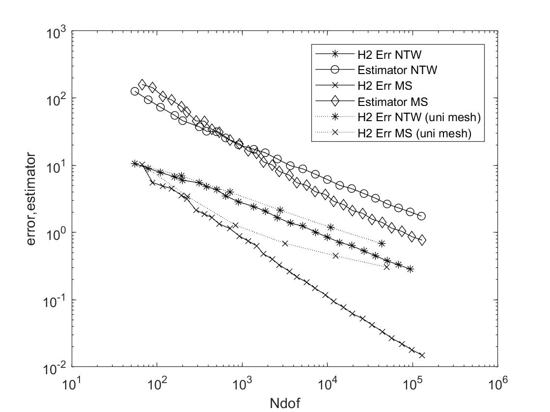
Figure 1. Convergence history for Example 1.

5.3. Example 2: Singularly perturbed problem on the square

In this example, we consider the unit square $\Omega=(0,1)^{2}$ and parameters $\alpha=1$, $\varepsilon=10^{-2}$. The exact solution

$$u=(\sin\pi x-\pi\varepsilon\frac{\cosh\frac{1}{2\varepsilon}-\cosh\frac{2x-1}{2\varepsilon}}{\sinh\frac{1}{2\varepsilon}})(\sin\pi y-\pi\varepsilon\frac{\cosh\frac{1}{2\varepsilon}-\cosh\frac{2y-1}{2\varepsilon}}{\sinh\frac{1}{2\varepsilon}})$$

has a boundary layer due to the incompatibility of the boundary condition with the limiting solution

$$\lim_{\varepsilon\rightarrow 0}u=\sin\pi x\sin\pi y.$$

Figure 2 displays the convergence history the absolute $\|\cdot\|_{a,h}$ norm errors and the error estimators $\eta$. Due to the boundary layer, the asymptotic convergence regime starts after approximately $2\,000$ degrees of freedom only. After that, the adaptive methods show the optimal convergence rate, which indicates that the layer has been resolved by the adaptive method. The optimal convergence rate with uniform refinement is observed starting from about $10^{4}$ degrees of freedom.

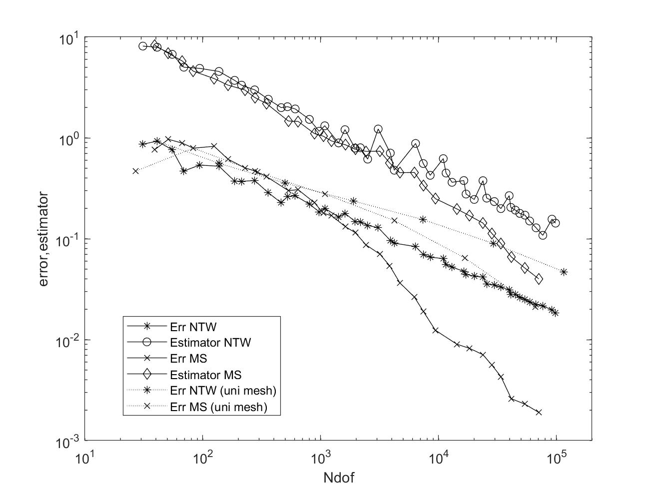
Figure 2. Convergence history for Example 2.

5.4. Example 3: Singularly perturbed problem on the L-shaped domain

We consider the L-shaped domain, $\alpha=1$ and $\varepsilon\in\{1/100,10^{-4}\}$ and the the right hand side $f(x,y)=(|x+y|)^{-1/3}$. In this example, no exact solution is known. Figure 3 and 4 display the convergence history the error estimators $\eta$. For the choice $\varepsilon=1/100$, both methods are observed to converge at the optimal rate. A mesh with $120\,577$ degrees of freedom generated with the MS element is displayed in Figure 5. For the more challenging choice $\varepsilon=10^{-4}$, all methods show only first-order rates within the range of numbers of degrees of freedom under consideration, which indicates that the boundary layer has not been resolved, yet.

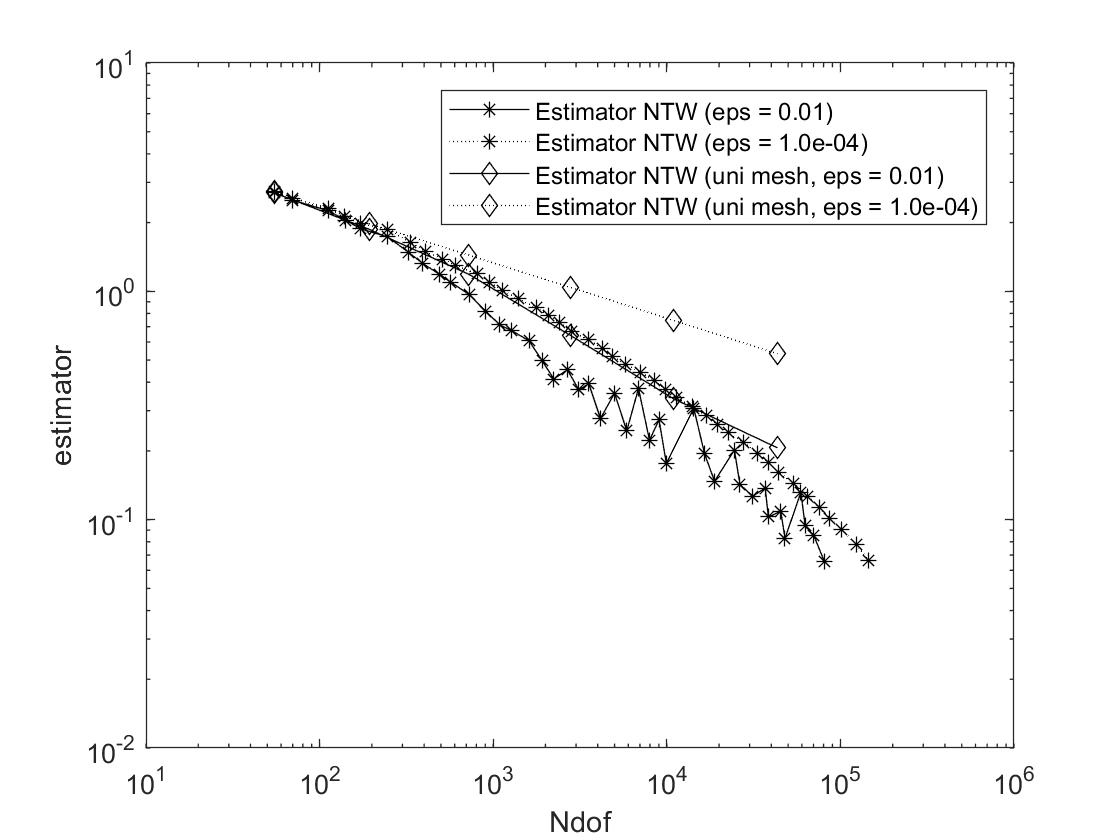
Figure 3. Values of the error and estimator for Example 3 with the NTW element.

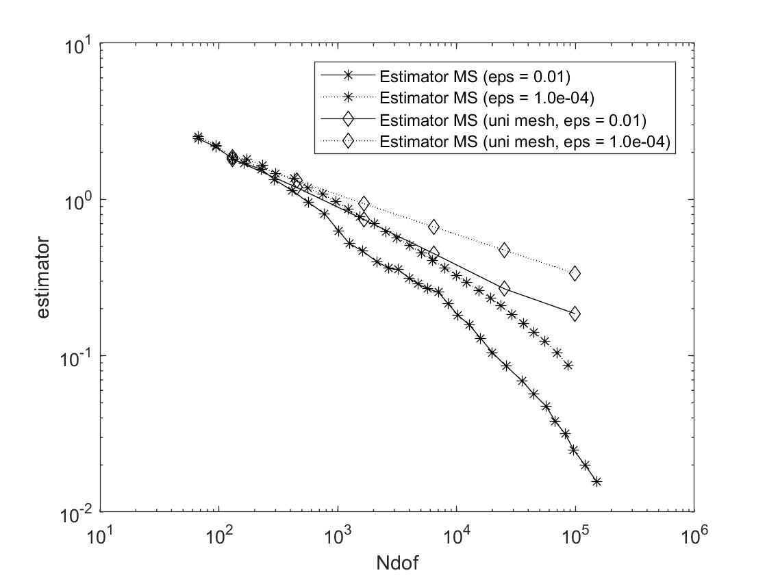
Figure 4. Values of the error and estimator for Example 3 with the MS element.

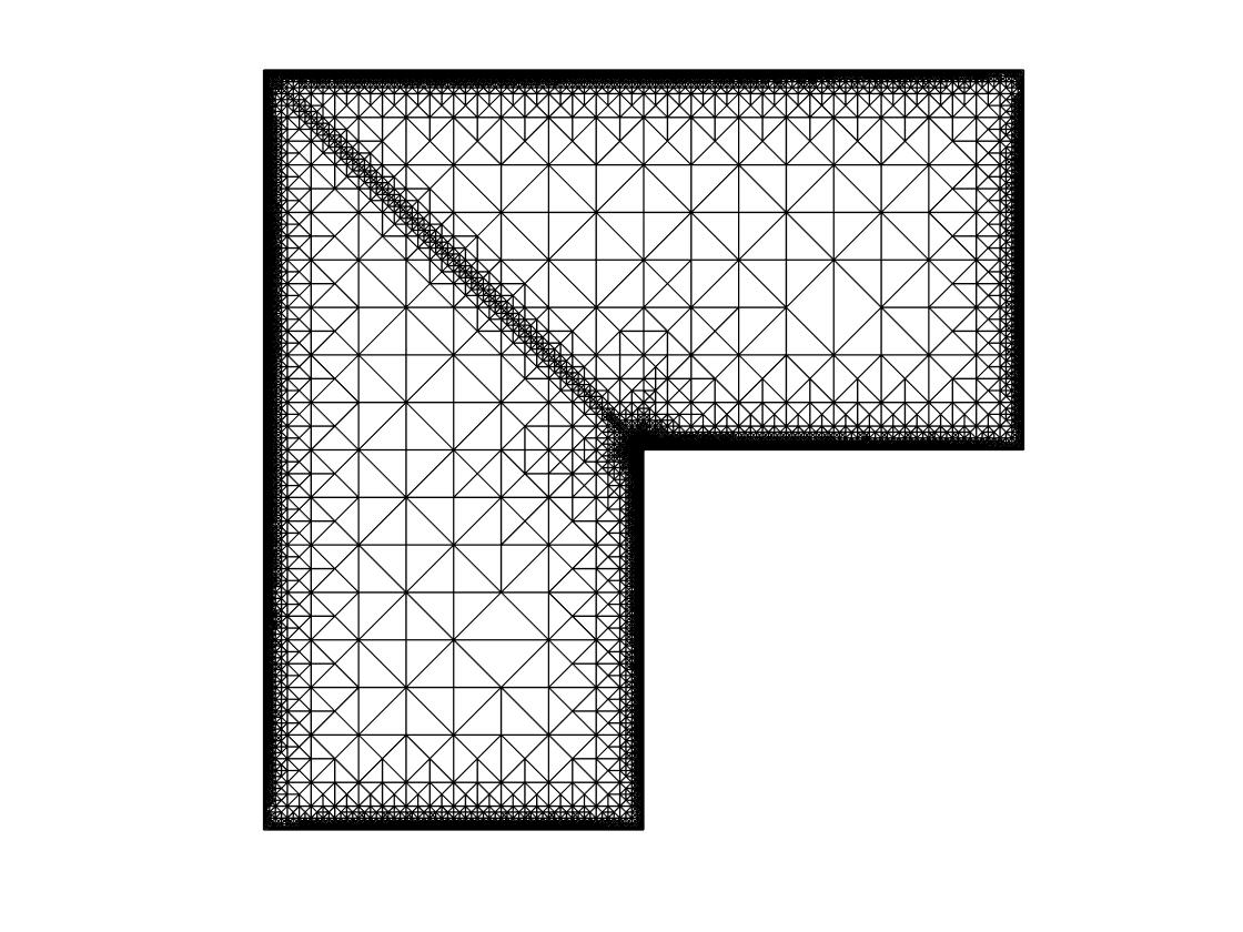
Figure 5. Adaptive mesh with 120 577 degrees of freedom generated by MS element when $\varepsilon=1/100$ in Example 3.

Appendix A Generalized Hsieh–Clough–Tocher elements

For $d=2$, the interpolation operator is defined on the HCT splits [23] and for $d=3$ on the Worsey–Farin splits [36]. The degrees of freedom for interpolation in the lowest order case (piecewise cubic) on both splits are the function value and the gradient value on the vertices and the directional derivatives at the midpoints in $d-1$ directions normal to the edge. The high order case can be found in [12, 15]. For convenient reading, we briefly describe the construction here.

Given a simplex $K\subseteq\mathbb{R}^{d}$ triangulated by a subdivision $\mathcal{T}_{K}$, we denote by $\mathcal{P}_{\ell}(\mathcal{T}_{K})$ the space of $C^{1}(K)$ functions that are piecewise polynomials of degree $\leq\ell$ with respect to $\mathcal{T}_{K}$. We furthermore denote

$$\tilde{\mathcal{P}}_{\ell}(\mathcal{T}_{K}):=\{v\in\mathcal{P}_{\ell}(\mathcal{T}_{K})|\nabla v|_{\partial K}=0\}\quad\text{and}\quad\tilde{\mathcal{P}}_{\ell,0}(\mathcal{T}_{K}):=\{v\in\tilde{\mathcal{P}}_{\ell}(\mathcal{T}_{K})|v_{\partial K}=0\}.$$

A.1. High order HCT element in 2D

Figure 6 shows an HCT split. The three vertices of the triangle $K$ are denoted as $a_{1},a_{2},a_{3}$ and the edge opposite to $a_{i}$ is denoted as $e_{i}$, $i=1,2,3$. Let as $c_{K}$ denote a given interior point of $K$. The sub-triangulation $\mathcal{T}_{K,c_{K}}^{\mathrm{HCT}}$ is formed by dividing $K$ in three sub-triangles $K_{i},i=1,2,3$, where $K_{i}$ is the convex hull of $c$ and $e_{i}$. The three interior edges $g_{i}$, $i=1,2,3$, are the line segments connecting $a_{i}$ and $c$. The high order ($\ell\geq 4$) HCT element is determined by the following degrees of freedom. A function $v\in\mathcal{P}_{\ell}(\mathcal{T}_{K,c_{K}}^{\mathrm{HCT}})$ is uniquely determined by

$$v(a_{i}),\nabla v(a_{i}),\quad v(c),\nabla v(c),$$

$$\fint_{e_{i}}vq_{\ell-4}\mathrm{d}s \text{ for all }q_{\ell-4}\in P_{\ell-4}(e_{i}),$$

$$\fint_{e_{i}}\partial_{n_{e_{i}}}vq_{\ell-3}\mathrm{d}s, \text{ for all }q_{\ell-3}\in P_{\ell-3}(e_{i}),$$

$$\fint_{g_{i}}\partial_{n_{g_{i}}}vq_{\ell-5}\mathrm{d}s,\leavevmode\nobreak\ \fint_{g_{i}}vq_{\ell-5}\mathrm{d}s \text{ for all }q_{\ell-5}\in P_{\ell-5}(g_{i}),$$

$$\fint_{K_{i}}vq_{\ell-6}\mathrm{d}s \text{ for all }q_{\ell-6}\in P_{\ell-6}(K_{i}),$$

for $i=1,2,3$. For proofs we refer to [8].

A.2. High order element in 3D on Worsey-Farin splits

The four vertices of the simplex $K$ are denoted as $a_{1},a_{2},a_{3},a_{4}.$ Let $c_{K}$ denote the midpoint of $K$. Let $F_{i}$ denote the face opposite to $a_{i}$. If $F_{i}$ is an interior face of the triangulation containing $K$, it is shared by two element $K$ and $K^{\prime}$, and $c_{i}\in F_{i}$ is defined as $c_{i}=\overline{c_{K}c_{K^{\prime}}}\cap F_{i}$, i.e., the intersection of the line connecting $c_{K}$ and $c_{K^{\prime}}$, and $F_{i}$. The Worsey–Farin split, dispayed in Figure 6, consists of the 12 simplices $[c_{K},a_{i},a_{j},c_{k}],\leavevmode\nobreak\ 1\leq i\neq j\neq k\leq 4$ and is denoted by $\mathcal{T}_{K}^{\mathrm{WF}}$. The high order ($\ell\geq 4$) Worsey–Farin element is determined by the following degrees of freedom. A function $v\in\mathcal{P}_{\ell}(\mathcal{T}_{K}^{\mathrm{WF}})$ is uniquely determined by

$$v(a_{m}),\nabla v(a_{m}),$$

$$\fint_{e_{i}}vq_{\ell-4}\mathrm{d}s \text{ for all }q_{\ell-4}\in P_{\ell-4}(e_{i}),$$

$$\fint_{e_{i}}\partial_{n_{e,j}}vq_{\ell-3}\mathrm{d}s \text{ for all }q_{\ell-3}\in P_{\ell-3}(e_{i}),$$

$$\fint_{F_{m}}(\nabla_{F_{m}}v\cdot g)dS \text{ for all }g\in\tilde{\mathcal{P}}_{\ell,0}(\mathcal{T}_{F_{m},c_{m}}^{\mathrm{HCT}}),$$

$$\fint_{F_{m}}(\partial_{n_{F_{m}}}v)g\mathrm{d}S \text{ for all }g\in\tilde{\mathcal{P}}_{\ell-1}(\mathcal{T}_{F_{m},c_{m}}^{\mathrm{HCT}}),$$

$$\fint_{T}\nabla v\cdot g\mathrm{d}x \text{ for all }g\in\nabla\tilde{\mathcal{P}}_{\ell,0}(\mathcal{T}_{K}^{\mathrm{W}F}).$$

for all $i=1,\dots,6$, $m=1,\dots,4$, and $j=1,2$. Here $\nabla_{F}$ is the surface gradient on $F$. The six edges of $K$ are denoted by $e_{1},\dots,e_{6}$, and $n_{e_{i},j},\leavevmode\nobreak\ j=1,2$ are two linear independent vectors orthogonal to the edge $e_{i}$. For proofs we refer to [15].

Figure 6. Hsieh–Clough–Tocher split (left) and Worsey–Farin split (right).

Appendix B Proof of Lemma 3.4

Without loss of generality we consider the most relevant case $\alpha=1$. We consider a $H^{2}$-conforming partition of unity with respect to the triangulation $\mathcal{T}$ and its vertices $\mathcal{N}$. This family $(\varphi_{y})_{y\in\mathcal{N}}$ consists of continuous and bounded functions and has the property $\sum_{y\in\mathcal{N}}\varphi_{y}=1$ in $\Omega$ and $\operatorname{supp}(\varphi_{j})=\overline{\omega}_{y}$ where $\omega_{y}$ is the vertex patch of diameter $h_{y}$. The partial derivatives satisfy

(B.1) $$\max_{\omega_{y}}|\partial^{\beta}\varphi_{y}|\lesssim h_{y}^{-|\beta|}$$

for any multi-index $\beta$ of length $|\beta|\leq 2$. Such partition is provided by the basis functions of a $H^{2}$-conforming finite element space with respect to $\mathcal{T}$ corresponding to the point evaluation in the vertices. Since any function of the format

$$v=\sum_{y\in\mathcal{N}}v_{y}\varphi_{y}$$

with functions $v_{y}\in V(\omega_{y})$ belongs to $V$, and since the functions $\varphi_{j}$ form a partition of unity, we can write

$$\min_{v\in V}\lvert\!\lvert\!\lvert u_{h}-v\rvert\!\rvert\!\rvert^{2}=\min_{(v_{y})_{y}\in V(\omega_{y})_{y}}\lvert\!\lvert\!\lvert\sum_{y\in\mathcal{N}}\varphi_{y}(u_{h}-v_{y})\rvert\!\rvert\!\rvert^{2}\lesssim\sum_{y\in\mathcal{N}}\min_{v_{y}\in V(\omega_{y})}\lvert\!\lvert\!\lvert\varphi_{y}(u_{h}-v_{y})\rvert\!\rvert\!\rvert^{2}$$

due to the bounded overlap of vertex patches. We abbreviate $w:=u_{h}-v_{y}$. From the product rule and the scaling (B.1) we infer

$$\lvert\!\lvert\!\lvert\varphi_{y}w\rvert\!\rvert\!\rvert^{2}\lesssim(h_{y}^{-2}+\varepsilon^{2}h_{y}^{-4})\|w\|_{0,\omega_{y}}^{2}+(1+\varepsilon^{2}h_{y}^{-2})\|\nabla_{h}w\|_{0,\omega_{y}}^{2}+\varepsilon^{2}\|D^{2}_{h}w\|_{0,\omega_{y}}^{2}.$$

From $(1+\varepsilon^{2}/h_{y}^{2})\leq 2\kappa_{y}^{-2}$ we deduce

$$\lvert\!\lvert\!\lvert\varphi_{y}w\rvert\!\rvert\!\rvert^{2}\lesssim h_{y}^{-2}\kappa_{y}^{-2}\|w\|_{0,\omega_{y}}^{2}+\kappa_{y}^{-2}\|\nabla_{h}w\|_{0,\omega_{y}}^{2}+\varepsilon^{2}\|D^{2}_{h}w\|_{0,\omega_{y}}^{2}.$$

The combination of the above arguments concludes the proof.

References

- [1] L. Beirão da Veiga, J. Niiranen, and R. Stenberg. A posteriori error estimates for the Morley plate bending element. Numer. Math., 106(2):165–179, 2007.
- [2] H. Blum and R. Rannacher. On mixed finite element methods in plate bending analysis. Comput. Mech., 6(3):221–236, 1990.
- [3] S. C. Brenner, T. Gudi, and L.-Y. Sung. An a posteriori error estimator for a quadratic -interior penalty method for the biharmonic problem. IMA J. Numer. Anal., 30(3):777–798, 2010.
- [4] C. Carstensen, D. Gallistl, and J. Hu. A posteriori error estimates for nonconforming finite element methods for fourth-order problems on rectangles. Numerische Mathematik, 124(2):309–335, 2013.
- [5] H. Chen, S. Chen, and Z. Qiao. -nonconforming tetrahedral and cuboid elements for the three-dimensional fourth order elliptic problem. Numer. Math., 124(1):99–119, 2013.
- [6] P. G. Ciarlet. The finite element method for elliptic problems, volume 40 of Classics in Applied Mathematics. Society for Industrial and Applied Mathematics (SIAM), Philadelphia, PA, 2002. Reprint of the 1978 original.
- [7] W. Dörfler. A convergent adaptive algorithm for Poisson’s equation. SIAM J. Numer. Anal., 33(3):1106–1124, 1996.
- [8] J. Douglas, Jr., T. Dupont, P. Percell, and R. Scott. A family of finite elements with optimal approximation properties for various Galerkin methods for 2nd and 4th order problems. RAIRO Anal. Numér., 13(3):227–255, 1979.
- [9] A. Ern and J.-L. Guermond. Finite elements I—Approximation and interpolation, volume 72 of Texts in Applied Mathematics. Springer, Cham, 2021.
- [10] D. Gallistl and S. Tian. Continuous finite elements satisfying a strong discrete Miranda–Talenti identity, 2022.
- [11] B. Gao, S. Zhang, and M. Wang. A note on the nonconforming finite elements for elliptic problems. J. Comput. Math., 29(2):215–226, 2011.
- [12] E. H. Georgoulis, P. Houston, and J. Virtanen. An a posteriori error indicator for discontinuous galerkin approximations of fourth-order elliptic problems. IMA Journal of Numerical Analysis, 31(1):281–298, 2011.
- [13] P. Grisvard. Singularities in boundary value problems, volume 22 of Recherches en Mathématiques Appliquées. Masson, Paris, 1992.
- [14] J. Guzmán, D. Leykekhman, and M. Neilan. A family of non-conforming elements and the analysis of Nitsche’s method for a singularly perturbed fourth order problem. Calcolo, 49(2):95–125, 2012.
- [15] J. Guzmán, A. Lischke, and M. Neilan. Exact sequences on Worsey–Farin splits. Mathematics of Computation, 91(338):2571–2608, 2022.
- [16] J. Hu and Z. C. Shi. A new a posteriori error estimate for the Morley element. Numer. Math., 112(1):25–40, 2009.
- [17] J. Hu, S. Tian, and S. Zhang. A family of 3D -nonconforming tetrahedral finite elements for the biharmonic equation. Sci. China Math., 63(8):1505–1522, 2020.
- [18] J. Hu and S. Zhang. An error analysis method SPP-BEAM and a construction guideline of nonconforming finite elements for fourth order elliptic problems. J. Comput. Math., 38(1):195–222, 2020.
- [19] P. Lascaux and P. Lesaint. Some nonconforming finite elements for the plate bending problem. Revue française d’automatique, informatique, recherche opérationnelle. Analyse numérique, 9(R1):9–53, 1975.
- [20] H. Li, P. Ming, and Z. C. Shi. The quadratic Specht triangle. J. Comput. Math., 38(1):103–124, 2020.
- [21] L. Morley. The triangular equilibrium element in the solution of plate bending problems. Aero. Quart., 19:149–169, 05 1968.
- [22] T. Nilssen, X. Tai, and R. Winther. A robust nonconforming -element. Math. Comp., 70(234):489–505, 2001.
- [23] P. Percell. On cubic and quartic Clough-Tocher finite elements. SIAM J. Numer. Anal., 13(1):100–103, 1976.
- [24] Z. C. Shi. On the convergence of the incomplete biquadratic nonconforming plate element. Math. Numer. Sinica, 8(1):53–62, 1986.
- [25] Z. C. Shi, S. C. Chen, and H. Huang. Plate elements with high accuracy. In Collection of papers on geometry, analysis and mathematical physics, pages 155–164. World Sci. Publ., River Edge, NJ, 1997.
- [26] Z. C. Shi and M. Wang. Finite Element Methods. Beijing: Science Press, 2013.
- [27] B. Specht. Modified shape functions for the three-node plate bending element passing the patch test. Internat. J. Numer. Methods Engrg., 26(3):705–715, 1988.
- [28] R. Verfürth. Robust a posteriori error estimators for a singularly perturbed reaction-diffusion equation. Numer. Math., 78(3):479–493, 1998.
- [29] R. Verfürth. A posteriori error estimation techniques for finite element methods. Oxford University Press, Oxford, 2013.
- [30] M. Wang and X. Meng. A robust finite element method for a 3-d elliptic singular perturbation problem. Journal of Computational Mathematics, pages 631–644, 2007.
- [31] M. Wang, Z. Shi, and J. Xu. A new class of zienkiewicz-type non-conforming element in any dimensions. Numer. Math., 106(2):335–347, 2007.
- [32] M. Wang, Z.-C. Shi, and J. Xu. Some -rectangle nonconforming elements for fourth order elliptic equations. J. Comput. Math., 25(4):408–420, 2007.
- [33] M. Wang and J. Xu. Minimal finite element spaces for -th-order partial differential equations in . Math. Comp., 82(281):25–43, 2013.
- [34] M. Wang, J. Xu, and Y. Hu. Modified Morley element method for a fourth order elliptic singular perturbation problem. J. Comput. Math., 24(2):113–120, 2006.
- [35] M. Wang, P. Zu, and S. Zhang. High accuracy nonconforming finite elements for fourth order problems. Sci. China Math., 55(10):2183–2192, 2012.
- [36] A. Worsey and G. Farin. An n-dimensional Clough-Tocher interpolant. Constructive Approximation, 3:99–110, 1987.
- [37] S. Zhang and M. Wang. A posteriori estimator of nonconforming finite element method for fourth order elliptic perturbation problems. J. Comput. Math., 26(4):554–577, 2008.