Expression Syntax Information Bottleneck
for Math Word Problems

Abstract.

Math Word Problems (MWP) aims to automatically solve mathematical questions given in texts. Previous studies tend to design complex models to capture additional information in the original text so as to enable the model to gain more comprehensive features. In this paper, we turn our attention in the opposite direction, and work on how to discard redundant features containing spurious correlations for MWP. To this end, we design an Expression Syntax Information Bottleneck method for MWP (called ESIB) based on variational information bottleneck, which extracts essential features of expression syntax tree while filtering latent-specific redundancy containing syntax-irrelevant features. The key idea of ESIB is to encourage multiple models to predict the same expression syntax tree for different problem representations of the same problem by mutual learning so as to capture consistent information of expression syntax tree and discard latent-specific redundancy. To improve the generalization ability of the model and generate more diverse expressions, we design a self-distillation loss to encourage the model to rely more on the expression syntax information in the latent space. Experimental results on two large-scale benchmarks show that our model not only achieves state-of-the-art results but also generates more diverse solutions. The code is available.

1. Introduction

Math Word Problems (MWP) is challenging and draws much attention from researchers in the field of natural language processing (Bobrow, 1964; Xiong et al., 2023) and information retrieval (e.g., mathematical understanding) (Huang et al., 2020; Zanibbi et al., 2021). MWP aims to automatically answer mathematical questions given in a natural language, which requires the model not only understand what facts are presented in a text, but also possess the reasoning capability to answer the mathematical question. Table 1 shows three examples of MWP with three mathematical problems and their solution expressions with answer.

Inspired by the success of deep learning (Wang et al., 2023; Pan et al., 2022), the encoder-decoder framework with attention mechanisms (Bahdanau et al., 2014) have been dominated in MWP (Wang et al., 2019, 2018a, 2018b), which bring the state-of-the-art to a new level. The key idea is to use an encoder to learn representations of problem text and employ a decoder to generate the corresponding solution expression and answer. Subsequently, several studies propose sequence-to-tree models, which explore the tree structure information presented in the text and improve the generation of solution expressions (Xie and Sun, 2019; Zhang et al., 2020b; Wu et al., 2021).

However, the previous MWP methods appear to rely on spurious correlations between the shallow heuristics in problem and solution expression (Patel et al., 2021). For example, as shown in Table 1, previous models may associate Problem 1 and Problem 2 with the mathematical formula “x$\times$y$\div$z”, since these two problems have similar semantic patterns, e.g., calculating the speed. Based on this association, the models could generate wrong solution expression for Problem 3 which has similar semantic problem expression like the text segment ”place A to place B” in Problems 1-2. In particular, the models that learn spurious correlations are more likely to generate wrong solution expression “$220\times 25\%\div 30\%$”, rather than “$220\div(25\%+30\%)$” for Problem 3. We define such a false association as spurious correlation. Some recent studies have revealed that MWP solvers relying on spurious correlations could achieve high accuracy (Patel et al., 2021; Kumar et al., 2021). These models can even compute correct answers without paying attention to the question part in the problem such as the text segment “how many kilometers is the total length of the two places?” in Problem 3 calculating the distance. In addition, the solution expression is sensitive to the perturbed latent representations (Liang and Zhang, 2021), since the semantically similar mathematical problems, even with totally different solution expressions and questions, can be encoded closely in the latent space. We believe it is an evidence that redundant information containing spurious correlations is encoded in the latent representation. Therefore, it is necessary to alleviate the spurious correlations by compressing the latent representations for math expressions while filtering latent-specific redundancy.

To solve the above challenges, we design a Expression Syntax Information Bottleneck method for MWP based on variational information bottleneck (VIB) (Alemi et al., 2016), which aims to discard redundant information containing spurious correlations (Fischer, 2020; Mukherjee et al., 2020). Our key idea is to encourage multiple models to predict the same math expression with different problem representations of the same problem so as to capture consistent information about expression syntax tree in expressions and discard latent-specific redundancy containing syntax-irrelevant information. In addition, we leverage mutual learning (Zhang et al., 2018) for learning variational information bottleneck, which can effectively reduce the latent-specific redundancy. Inspired by the observation that there are usually multiple solutions to solve a problem, we also design a self-distillation loss which encourages the decoder to rely on the syntax information in latent space, enabling the model to generate diverse solutions.

We summarize our main contributions as follows. (1) We are the first to reduce spurious correlations so as to improve the performance of MWP. (2) We propose a novel expression syntax information bottleneck method for MWP, which extracts essential syntax information of math expression and filters redundant information containing spurious correlations. (3) We design a self-distillation loss to encourage the model to generate more diverse solution expressions. (4) Extensive experiments on two benchmark datasets show that our model outperforms the strong baselines in a noticeable margin.

Table 1. Three examples of MWP.

Problem 1: From place A to place B, if a bicycle travels 16 kilometers per hour, it can be reached in 4 hours. If it only takes 2 hours by car, how many kilometers per hour does the car travel?
Solution Expression 1: 16$\times$4$\div$2  Answer: 32
Problem 2: Uncle Jack drove from place A to place B, and it took 6 hours to arrive at the speed of 70 kilometers per hour. When I returned, I accelerated the speed due to the task. It only took 4 hours to return to the first place. What was the speed when I returned?
Solution Expression 2: 70$\times$6$\div$4  Answer: 105
Problem 3: A car travels 25% of the whole journey from place A to place B in the first hour, 30% of the whole journey in the second hour, a total of 220 kilometers in two hours, how many kilometers is the total length of the two places?
Solution Expression 3: $220\div(25\%+30\%)$  Answer: 400
Wrong Solution Expression 3: $220\times 25\%\div 30\%$

2. Methodology

A math word problems (MWP) can be denoted by a projection $F:x\mapsto z\mapsto y$, where ${x}=\{w_{1},w_{2},\dots,w_{m}\}$ is the problem sequence with $m$ words, $z$ is the compressed representation of the original problem $x$ and $y=\{o_{1},o_{2},\dots,o_{n}\}$ is the solution expression of the problem with $n$ words. The goal of MWP is to establish a model $F$ which generates a correct solution expression $y$ and calculates the correct answer for the problem $x$.

As illustrated in Figure 1, the proposed ESIB is composed of a source network (denoted as SN) and a collaborator network (denoted as CN). The two networks are optimised collaboratively and capture consistent information across different problem representations throughout the training process. We use the deep variational information bottleneck (VIB) framework as the backbone of both SN and CN. The VIB aims to generate problem representation $z\in\mathbb{R}^{s}$ by compressing and discarding redundant information in latent representation $v\in\mathbb{R}^{d}$ without reducing essential information related to the target $y$, where $d$ denotes hidden size of decoder and $s$ denotes the dimension of problem representation. So the above projection $F$ can be rewritten as $F:x\mapsto v\mapsto z\mapsto y$, where $v$ denotes latent representation and $z$ denotes problem representation sampled from $e^{\mu}(v)\sim N\left(e^{\mu}(v),e^{\sigma}(v)\right)$ ($e$ denotes a dense layer).

2.1. Encoder-Compressor-Decoder Architecture

Encoder

We adopt the RoBERTa model (Liu et al., 2019) as our encoder. We pass the problem sequence $x$ into the RoBERTa model and obtain latent representation $v$ ([CLS] vector output by the pre-trained language model (PLM) and its dimension is converted from 768 to $d$ by a dense layer). In order to model the relationship between the quantities in the PLM, we set up a learnable quantity embedding matrix $\emph{Q}_{t}=\{q_{1},q_{2},\dots,q_{n}\}$, similar to the learnable position embedding in BERT (Devlin et al., 2018). When passing the sequence $x$ into the encoder, we replace the each quantity in the sequence $x$ (i.e., the numbers in the problem) with a embedding $q_{i}\in\emph{Q}_{t}$.

Compressor

Our model takes the encoder output $v$ and feeds it into a variational information bottleneck (Alemi et al., 2016) module which outputs a sampled vector $z$. This part removes redundant information by optimizing a variational upper bound $\mathcal{V}_{IB}$. We will detail how to optimize $\mathcal{V}_{IB}$ in Section 2.2.

Figure 1. Overview of the proposed method ESIB.

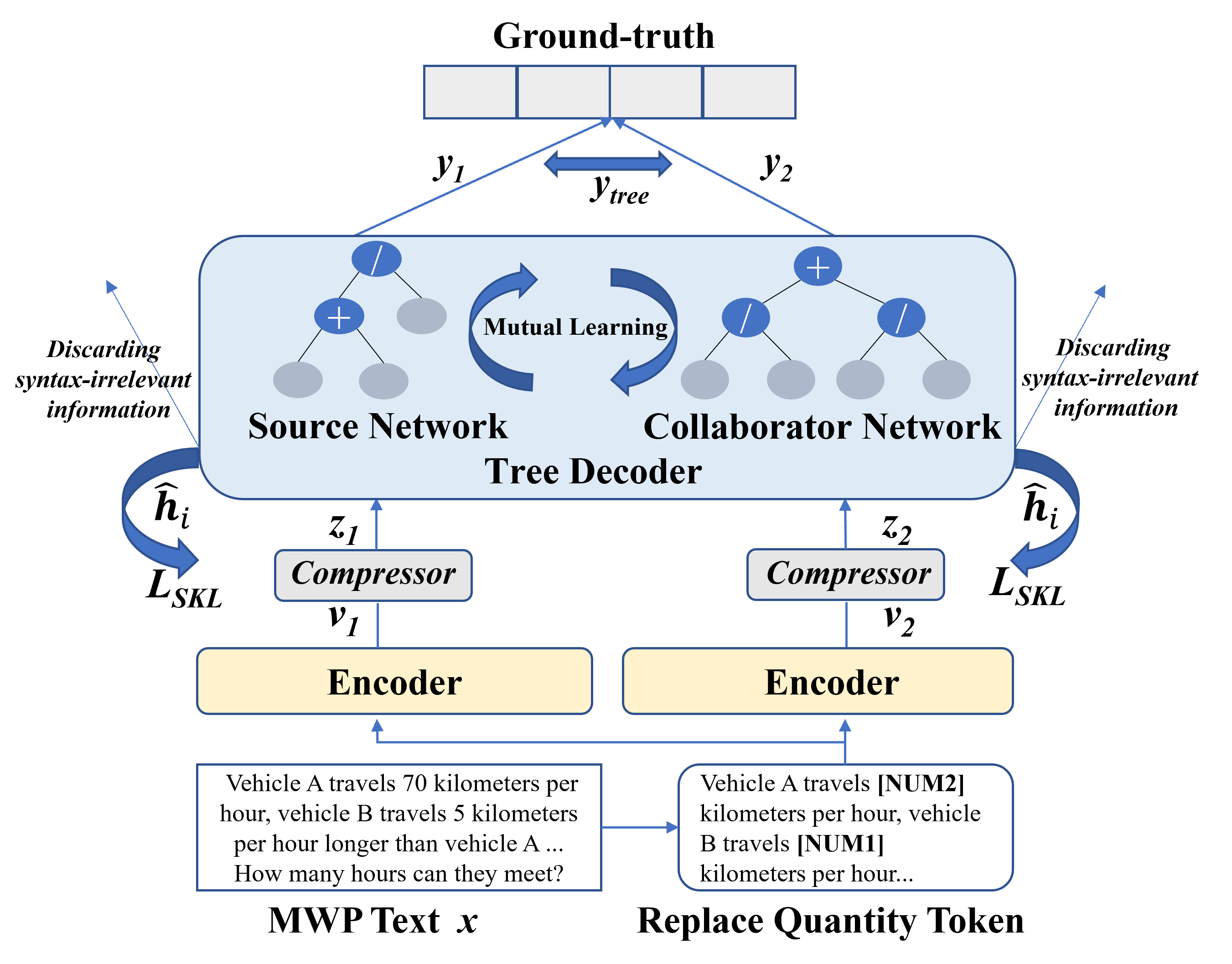
Decoder

Our decoder follows the GTS model (Xie and Sun, 2019). We use the sampled representation $z$ to initialize the initial state of the decoder and the recursive operation of the decoder to construct $y$ by the order of pre-order traversal. First, the root node $q_{\rm root}$ (middle operator part) is first generated. Then, we generate the left child node $q_{l}$. Finally, we generate the right child node $q_{r}$. This process has been iterated until the leaf nodes are generated. The attention mechanism is applied to learn the global context vector $G_{i}$ which is utilized to generate the current node token $\hat{y}_{i}$. Here we denote the digital embedding after being encoded by the encoder as $Q$. Mathematically, we define the attention mechanism as follows:

(1) $$G_{i}=\left\{\begin{array}[]{lll}\text{ Attention }(x,\emph{q}_{\rm root},\emph{q}_{l}),\ \ \emph{q}_{l}\notin\emptyset.\\ \text{ Attention }(x,\emph{q}_{\rm root},\emph{q}_{sl}),\ \ \emph{q}_{sl}\notin\emptyset.\\ \text{ Attention }(x,\emph{q}_{\rm root}),\ \ \emph{q}_{l},\emph{q}_{sl}\in\emptyset.\end{array}\right.$$

(2) $$\hat{y}_{i},\hat{h}_{i}={\rm Predict}(G_{i},Q),$$

where ${\rm Predict}(\cdot)$ is prediction layer for producing tree nodes $\hat{y}_{i}$ and hidden state of decoding step $i$ (denoted as $\hat{h}_{i}\in\mathbb{R}^{d}$).

If the current node is an operator, we will generate the left and right child nodes and push them into the stack in the tree decoder according to the top-down method. If it is a number, we will perform the merge operation until the leaf nodes in the stack pop out, and the result of the merge is pushed into the left child node stack for attention operation. The merge operation will pop the required node $\emph{q}_{\rm op}$ and $\emph{q}_{\rm subtree}$ from an embedding stack. Finally, the merge operation outputs the answer of the mathematical expression. This recursive construction process can be defined as follows:

(3) $$q_{l}={\rm Left}(\hat{G},\hat{y_{i}},q_{\rm root}).$$

(4) $$q_{r}={\rm Right}(\hat{G},\hat{y_{i}},q_{\rm root}).$$

(5) $$q_{m}={\rm Merge}(q_{\rm op},q_{\rm subtree},q_{m-1}).$$

2.2. Information Bottleneck

Our ESIB method is driven by Information Bottleneck (IB) (Tishby et al., 2000; Alemi et al., 2016) that forces features to be concise by filtering the task-irrelevant information (i.e., syntax-irrelevant spurious correlations for MWP). Specifically, suppose we know the joint distribution $p(x,y)$, our goal is to learn a problem representation $z$ that maximizes its predictive power for generating $y$, subject to the constraints of the amount of information it carries about $x$:

(6) $$\mathcal{L}_{IB}=I(y;z)-\lambda I(x;z),$$

where $I(\cdot;\cdot)$ denotes the mutual information. $\lambda$ is a Lagrangian multiplier that controls the trade-off between the sufficiency (the task performance quantified by $I(y;z)$) and the minimality (the complexity of the representation quantified by $I(x;z)$). In this paper, we focus on compressing the redundancy in latent representation $v$ (denoted as a substitute for the problem $x$). Following (Alemi et al., 2016), Equation (6) can be variationally upper bounded by:

(7) $$\begin{aligned} \mathcal{V}_{IB}=\frac{1}{N}\sum_{n=1}^{N}\left\{\lambda D_{\mathrm{KL}}\left(e\left(z\mid v^{n}\right)\|b(z)\right)-\mathbb{E}_{\epsilon}\log d\left(y^{n}\mid e\left(z^{n},\epsilon\right)\right)\right\}\end{aligned},$$

where $N$ is the number of data, $e\left(z^{n},\epsilon\right)$ transforms the $z$ into initial state of the decoder (denoted as $\bar{z}\in\mathbb{R}^{m\cdot d}$) and $e\left(z\mid v^{n}\right)$ transforms the representation $v$ into two tensors: $e^{\mu}(v)$ denotes the features-mean and $e^{\sigma}(v)$ denotes the diagonal features-covariance. We use the reparameterization to obtain the compressed representation $z=e(v,\epsilon)=e^{\mu}(v)+\epsilon e^{\sigma}(v)$ with $\epsilon\sim N(0,1)$. The prior distribution of $z$ (denoted as $b(z)$) is a standard normal distribution. The decoder $d$ converts the sampled representation $z$ into a mathematical expression $y$, and calculates the answer.

With the compression capability of VIB, it is possible to lose the necessary information about the target $y$ in the feature $z$ when optimizing the trade-off between the compression and redundancy. We will introduce how to identify the syntax-irrelevant information in Section 2.3.

2.3. Latent-specific Redundancy

In this section, we demonstrate that the latent-specific redundancy containing syntax-irrelevant information can be effectively reduced by using mutual learning (Zhang et al., 2018). Inspired by the method forcing two networks to learn from each other (Zhang et al., 2018), we encourage two networks to produce compressed representation $z$ filtered latent-specific redundancy for keeping all predictive information about expression syntax trees in expression $y$ by passing an representation of expression syntax tree (denoted as $y_{tree}$ obtained by concatenating each $\hat{h}_{i}$ defined in equation(2) when decoder predicts the expression syntax tree of the math expression) to each other.

We attempt to learn a vector $z$ that contains expression syntax tree information about solution expression $y$ as much as possible and achieve this goal by optimizing the mutual information of $v$ and $z$. We take CN as an example, and factorize the mutual information (Federici et al., 2020) between $v_{1}$ and $z_{1}$ as follows:

(8) $$I\left(v_{1};z_{1}\right)=\underbrace{I\left(v_{1};z_{1}\mid v_{2}\right)}_{\text{Latent-specific Redundancy }}+\underbrace{I\left(v_{2};z_{1}\right)}_{\text{Consistent Information}},$$

where $v_{1}$ and $z_{1}$ denote latent and problem representation for CN respectively; $v_{2}$ and $z_{2}$ denote that of SN. $I\left(v_{1};z_{1}\mid v_{2}\right)$ indicates that the information contained in $z_{1}$ is unique to $v_{1}$ and cannot be inferred by representation $v_{2}$ (Federici et al., 2020). We call $I\left(v_{1};z_{1}\mid v_{2}\right)$ as latent-specific redundancy or syntax-irrelevant information. It can be discarded by minimizing $I\left(v_{1};z_{1}\mid v_{2}\right)$(Federici et al., 2020) which can be upper bounded by the following inequality:

(9) $$I\left(v_{1};z_{1}\mid v_{2}\right)=\mathbb{E}_{v_{1},v_{2}\sim S_{1}(v\mid x)}\mathbb{E}_{z_{1},z_{2}\sim S_{2}(z\mid v)}\left[\log\frac{p\left(z_{1}\mid v_{1}\right)}{p\left(z_{1}\mid v_{2}\right)}\right]$$

$$=\mathbb{E}_{v_{1},v_{2}\sim S_{1}(v\mid x)}\mathbb{E}_{z_{1},z_{2}\sim S_{2}(z\mid v)}\left[\log\frac{p\left(z_{1}\mid v_{1}\right)p\left(z_{2}\mid v_{2}\right)}{p\left(z_{2}\mid v_{2}\right)p\left(z_{1}\mid v_{2}\right)}\right]$$

$$=D_{KL}\left[p\left(z_{1}\mid v_{1}\right)\|p\left(z_{2}\mid v_{2}\right)\right]-D_{KL}\left[p\left(z_{2}\mid v_{1}\right)\|p\left(z_{2}\mid v_{2}\right)\right]$$

$$\leq D_{KL}\left[p\left(z_{1}\mid v_{1}\right)\|p\left(z_{2}\mid v_{2}\right)\right].$$

Inspired by (Federici et al., 2020), we approximate the upper bound above by replacing $z$ with $y_{tree}$. Since $y_{tree}$ generated from $z$ contains all the information of the representation $z$ and all the latent-specific redundancy to be discarded. In addition, the parameters to be optimized about $z$ are included in the decoder. Considering the above points, we utilize $D_{\mathrm{KL}}\left(\mathbb{P}_{z_{1}}\|\mathbb{P}_{z_{2}}\right)$ ($\mathbb{P}_{z_{1}}$ denotes $p\left(y_{{tree}_{1}}\mid z_{1}\right)$ and $\mathbb{P}_{z_{2}}$ denotes $p\left(y_{{tree}_{2}}\mid z_{2}\right)$ right) as an upper bound to approximate $D_{KL}\left[p\left(z_{1}\mid v_{1}\right)\|p\left(z_{2}\mid v_{2}\right)\right]$. Similarly, we can use $D_{\mathrm{KL}}\left(\mathbb{P}_{z_{2}}\|\mathbb{P}_{z_{1}}\right)$ to minimize $I\left(v_{2};z_{2}\mid v_{1}\right)$ for SN. We introduce the objective $\mathcal{L}_{SKL}$ to minimize the latent-specific redundancy for both $z_{1}$ and $z_{2}$:

(10) $$\small\mathcal{L}_{SKL}=\min_{\theta,\phi}\mathbb{E}_{v_{1},v_{2}\sim E_{\theta}(v\mid x)}\mathbb{E}_{z_{1},z_{2}\sim E_{\phi}(z\mid v)}\left[D_{SKL}\left[\mathbb{P}_{z_{1}}\|\mathbb{P}_{z_{2}}\right]\right]$$

where $\theta$ and $\phi$ denote the parameters of CN and SN. The two networks are optimized alternately during training. $\mathbb{P}_{z_{1}}=p_{\theta}\left(y_{1}\mid z_{1}\right)$ and $\mathbb{P}_{z_{2}}=p_{\phi}\left(y_{2}\mid z_{2}\right)$ denote the concatenation of the output distributions at each step of the model prediction of CN and SN respectively. $D_{SKL}$ denotes symmetrized KL divergence obtained by averaging the expected value of $D_{\mathrm{KL}}\left(\mathbb{P}_{z_{1}}\|\mathbb{P}_{z_{2}}\right)$ and $D_{\mathrm{KL}}\left(\mathbb{P}_{z_{2}}\|\mathbb{P}_{z_{1}}\right)$. We calculate this loss by mutual learning (Zhang et al., 2018) between CN and SN. In the mutual learning setup, in an iteration, the model will compute $\mathcal{L}_{SKL_{1}}$ and $\mathcal{L}_{SKL_{2}}$ for CN and SN respectively. In addition, we need to maximize $I\left(v_{2};z_{1}\right)$ to ensure that the compressed representation $z_{1}$ has enough information to predict $y$. We use the chain rule to decompose $I\left(v_{2};z_{1}\right)$ into the following two terms:

(11) $$I\left(v_{2};z_{1}\right)=\underbrace{I\left(v_{2};z_{1}\mid y\right)}_{\text{Redundancy }}+\underbrace{I\left(z_{1};y\right)}_{\text{Predictive Information}},$$

where $y$ represents ground-truth solution expression. In practice, we can maximize $I\left(z_{1};y\right)=\mathbb{E}_{\epsilon}\log d\left(y^{n}\mid e\left(x^{n},\epsilon\right)\right.$ (included in $\mathcal{V}_{IB}$) which is calculated to compress redundant information $I\left(v_{2};z_{1}\mid y\right)$ and indirectly maximize $I\left(v_{2};z_{1}\right)$. Ideally, $I\left(v_{2};z_{1}\mid y\right)$ should be zero. As suggested in (Federici et al., 2020), we minimize latent-specific redundancy by jointly minimizing $I\left(v_{1};z_{1}\mid v_{2}\right)$ and maximizing $I\left(v_{2};z_{1}\right)$. We define the redundancy terms in Eq. (8) and Eq. (11) as the syntax-irrelevant information.

2.4. Self-distillation Loss

In this section, we introduce a novel self-distillation loss to increase the diversity of generated expressions. Suggested by (Fischer, 2020), the $I(v;z\mid y)$ in conditional information bottleneck can be variationally upper bounded by:

(12) $$D_{\mathrm{KL}}\left(e\left(z\mid v^{n}\right)\|b\left(z\mid y^{n}\right)\right),$$

where $e\left(z\mid v^{n}\right)$ defined in equation (2) is moved towards the conditional marginal $b^{\mu}(y)\sim N\left(b^{\mu}(y),b^{\sigma}(y)\right)$. We modify equation (12) as:

(13) $$\mathcal{V}_{SDL}=\frac{1}{N}\sum_{n=1}^{N}D_{SKL}\left(\bar{y}\|\bar{z}\right),$$

where $\bar{y}$ denotes that averaging the all $\hat{h}_{i}$. Intuitively, $\mathcal{V}_{SDL}$ make the decoder more rely on latent space of $z$ which contains expression syntax tree information for all expressions when predicting expression $y$. Benefiting from the randomness of $z$, the model can generate more diverse solution expressions. Finally, we calculate the loss functions $\mathcal{L}_{1}$ for SN and $\mathcal{L}_{2}$ for CN as follows:

(14) $$\mathcal{L}_{1}=\mathcal{V}_{IB_{1}}+\mathcal{V}_{SDL_{1}}+\alpha\times\mathcal{L}_{SKL_{1}}.$$

(15) $$\mathcal{L}_{2}=\mathcal{V}_{IB_{2}}+\mathcal{V}_{SDL_{2}}+\alpha\times\mathcal{L}_{SKL_{2}}.$$

where $\alpha$ is a proportional coefficient. $\mathcal{V}_{IB_{1}}$, $\mathcal{V}_{SDL_{1}}$, $\mathcal{L}_{SKL_{1}}$ are the training objectives for SN. $\mathcal{V}_{IB_{2}}$, $\mathcal{V}_{SDL_{2}}$, $\mathcal{L}_{SKL_{2}}$ are the training objectives for CN. Based on empirical observation, although $\mathcal{V}_{SDL}$ can increase the diversity of solution expressions, it also reduces accuracy of the final answer.

3. Experimental Setup

Datasets

We conduct experiments on two benchmark MWP datasets: Math23k (Wang et al., 2017) and Ape210k (Zhao et al., 2020). Math23k contains 22162/1000 questions for training/testing, respectively. Ape210k is composed of 166,270 questions for training, 4,157 questions for validation, and 4,159 questions for testing.

Implementation Details

The word embedding size of decoder is set to 1024 and proportional coefficient $\alpha$ in loss function is set to 0.005. We set the dimension of vectors $z$ to 50. When the encoder is BERT, we set the dimension of $z$ to 32. We adopt RoBERTa (Liu et al., 2019) as the problem encoder. Following RoBERTa’s setting, the hidden size of the encoder is set to 768, and we set the hidden size of the decoder to 1024. We used Adamw (Loshchilov and Hutter, 2018) as the optimizer with the learning rate as 5e-5. The mini-batch size is set to 16. We adopt a beam search with the size of 5. Dropout (dropout rate = 0.5) is employed to avoid overfitting. For Ape210K, we set the maximum sequence length of questions as 150 and that of solution expressions as 50, similar to (Wu et al., 2021). Our model takes 80 epochs on Math23k and 50 epochs on Ape210k for convergence.

Baselines

We compare our model with several strong baseline methods, including NumS2T (Wu et al., 2021), TSN-MD (Zhang et al., 2020a), MATH-EN (Wang et al., 2018a), Multi-E/D (Shen and Jin, 2020), GTS (Xie and Sun, 2019), StackDecoder (Chiang and Chen, 2018), KAS2T (Wu et al., 2021), Graph2tree (Zhang et al., 2020b), and Ape (Zhao et al., 2020).

4. Experimental Results

4.1. Main Results

The evaluation metric is answer accuracy. Table 2 show the performance comparison of our model with baseline methods on Math23K and Ape210k, respectively. In Table 2, since there is a trade-off between the variety of expressions and the correctness of the answer, we do not add ${V}_{SDL}$ into the source network (SN) and the collaborator network (CN). From Table 2 we can observe that our models (both CN and SN) achieve consistently and substantially better performance than the compared methods. In addition, the accuracy of CN is higher than that of SN. This is because, in one iteration, CN is provided with $y_{tree}$ predicted by SN when SN has not been trained by ground-truth then SN is provided with $y_{tree}$ predicted by CN when CN has been trained by ground-truth.

We also measure the accuracy of solution expression. We consider a solution expression as correct when the predicted expression exactly matches the ground truth solution. Generally, the mathematical expression generated by the tree decoder conforms to the syntactic specification. As long as the answer obtained by the expression operation is consistent with the ground-truth, then we consider the expression to be a valid solution. We take the subtraction value between answer accuracy (denoted as Answer-Acc) and solution expression accuracy (denoted as Expression-Acc) as the diversity evaluation metric (denoted as Diversity) of the generated solution expressions. As shown in Table 3, our model can generate more diverse solution expressions that are not included in ground-truth expressions. As expected, the model with $\mathcal{V}_{SDL}$ has better diversity but lower answer accuracy.

Table 2. Solution accuracy of ESIB and various baselines. Note that Math23K denotes results on public test set.

Models	Math23k	Ape210k
StackDecoder	-	52.2
GTS	75.6	67.7
KAS2T	76.3	68.7
TSN-MD	77.4	-
Graph2Tree	77.4	-
Ape	-	70.2
NumS2T	78.1	70.5
Multi-E/D	78.4	-
SN	84.2	76.3
CN	85.9	76.8

Table 3. Accuracy of diversity generation on Math23k with Self-distillation Loss.

Models	Answer-Acc	Equation-Acc	Diversity
MATH-EN	66.7	60.1	6.6
GTS	75.6	64.8	10.8
TSN-MD	77.4	65.8	11.6
CN with $\mathcal{V}_{SDL}$	85.4	71.9	13.5
CN	85.9	73.5	12.4

Table 4. Ablation study on Math23k.

Models	Math23k
CN	85.9
CN w/o MT	85.2
CN w/o VIB	84.8
CN w/o MT+VIB	83.1
CNBERT	84.3
CNBERT w/o MT+VIB	82.4

Table 5. Case study from Math23k. Demonstrates the ability of the model to generate multiple solutions.

Problem Text:	A train leaves from place A at 7 o’clock and arrives at place B at 17 o’clock. The train travels 75 kilometers per hour. How many kilometers is the distance between the two places?
Ground-truth:	(17 $-$ 7) $\times$ 75
Source Network:	(17 $-$ 7) $\times$ 75
Collaborator Network:	17 $\times$ 75 $-$ 7 $\times$ 75

4.2. Ablation Study

We conduct ablation test on Math23k to analyze the impact of different components in ESIB. Since the best results are produced by CN, we only conduct ablation study on CN. First, we remove the mutual learning, denoted as CN w/o MT. Second, we remove the VIB from SN and CN to evaluate the impact of VIB (denoted as CN w/o VIB). In addition, we report the results by removing both MT and VIB (denoted as CN w/o MT+VIB). To evaluate the impact of the pre-training model, we also replaced the RoBERTa encoder with BERT (Devlin et al., 2018) (denoted as CN_BERT). We summarize the results in Table 4. Both the VIB strategy and mutual learning contribute greatly to the performance of ESIB.

4.3. Case Study

As an intuitive way to show the performance of ESIB, we randomly choose one problem form Math23k and show its solution expression generated by our model. As shown in Table 5, we observe that our model can produce two different but equivalent solutions. In addition, our model can correctly solve the problems in Table 1, which proves that our model does effectively reduce spurious correlations.

5. Conclusion

In this paper, we proposed an expression syntax information bottleneck method for MWP with mutual learning, which discards redundant features containing spurious correlations. Furthermore, we designed a self-distillation loss to encourage the model to rely more on the syntax information in the latent space. Extensive experiments on two benchmark MWP datasets demonstrated the effectiveness of our model.

References

- (1)
- Alemi et al. (2016) Alexander A Alemi, Ian Fischer, Joshua V Dillon, and Kevin Murphy. 2016. Deep variational information bottleneck. arXiv preprint arXiv:1612.00410 (2016).
- Bahdanau et al. (2014) Dzmitry Bahdanau, Kyunghyun Cho, and Yoshua Bengio. 2014. Neural machine translation by jointly learning to align and translate. arXiv preprint arXiv:1409.0473 (2014).
- Bobrow (1964) Daniel G Bobrow. 1964. Natural language input for a computer problem solving system. (1964).
- Chiang and Chen (2018) Ting-Rui Chiang and Yun-Nung Chen. 2018. Semantically-aligned equation generation for solving and reasoning math word problems. arXiv preprint arXiv:1811.00720 (2018).
- Devlin et al. (2018) Jacob Devlin, Ming-Wei Chang, Kenton Lee, and Kristina Toutanova. 2018. Bert: Pre-training of deep bidirectional transformers for language understanding. arXiv preprint arXiv:1810.04805 (2018).
- Federici et al. (2020) Marco Federici, Anjan Dutta, Patrick Forré, Nate Kushman, and Zeynep Akata. 2020. Learning robust representations via multi-view information bottleneck. arXiv preprint arXiv:2002.07017 (2020).
- Fischer (2020) Ian Fischer. 2020. The conditional entropy bottleneck. Entropy 22, 9 (2020), 999.
- Huang et al. (2020) Zhenya Huang, Qi Liu, Weibo Gao, Jinze Wu, Yu Yin, Hao Wang, and Enhong Chen. 2020. Neural mathematical solver with enhanced formula structure. In Proceedings of the 43rd International ACM SIGIR Conference on Research and Development in Information Retrieval. 1729–1732.
- Kumar et al. (2021) Vivek Kumar, Rishabh Maheshwary, and Vikram Pudi. 2021. Adversarial Examples for Evaluating Math Word Problem Solvers. arXiv preprint arXiv:2109.05925 (2021).
- Liang and Zhang (2021) Zhenwen Liang and Xiangliang Zhang. 2021. Solving Math Word Problems with Teacher Supervision. IJCAI (2021).
- Liu et al. (2019) Yinhan Liu, Myle Ott, Naman Goyal, Jingfei Du, Mandar Joshi, Danqi Chen, Omer Levy, Mike Lewis, Luke Zettlemoyer, and Veselin Stoyanov. 2019. Roberta: A robustly optimized bert pretraining approach. arXiv preprint arXiv:1907.11692 (2019).
- Loshchilov and Hutter (2018) Ilya Loshchilov and Frank Hutter. 2018. Fixing weight decay regularization in adam. (2018).
- Mukherjee et al. (2020) Sudipto Mukherjee, Himanshu Asnani, and Sreeram Kannan. 2020. CCMI: Classifier based conditional mutual information estimation. In Uncertainty in artificial intelligence. PMLR, 1083–1093.
- Pan et al. (2022) Yu Pan, Zeyong Su, Ao Liu, Jingquan Wang, Nannan Li, and Zenglin Xu. 2022. A Unified Weight Initialization Paradigm for Tensorial Convolutional Neural Networks. In ICML (Proceedings of Machine Learning Research, Vol. 162). PMLR, 17238–17257.
- Patel et al. (2021) Arkil Patel, Satwik Bhattamishra, and Navin Goyal. 2021. Are NLP Models really able to Solve Simple Math Word Problems? arXiv preprint arXiv:2103.07191 (2021).
- Shen and Jin (2020) Yibin Shen and Cheqing Jin. 2020. Solving math word problems with multi-encoders and multi-decoders. In Proceedings of the 28th International Conference on Computational Linguistics. 2924–2934.
- Tishby et al. (2000) Naftali Tishby, Fernando C Pereira, and William Bialek. 2000. The information bottleneck method. arXiv preprint physics/0004057 (2000).
- Wang et al. (2018a) Lei Wang, Yan Wang, Deng Cai, Dongxiang Zhang, and Xiaojiang Liu. 2018a. Translating a math word problem to an expression tree. arXiv preprint arXiv:1811.05632 (2018).
- Wang et al. (2018b) Lei Wang, Dongxiang Zhang, Lianli Gao, Jingkuan Song, Long Guo, and Heng Tao Shen. 2018b. Mathdqn: Solving arithmetic word problems via deep reinforcement learning. In Proceedings of the AAAI Conference on Artificial Intelligence, Vol. 32.
- Wang et al. (2019) Lei Wang, Dongxiang Zhang, Jipeng Zhang, Xing Xu, Lianli Gao, Bing Tian Dai, and Heng Tao Shen. 2019. Template-based math word problem solvers with recursive neural networks. In Proceedings of the AAAI Conference on Artificial Intelligence, Vol. 33. 7144–7151.
- Wang et al. (2023) Maolin Wang, Yu Pan, Xiangli Yang, Guangxi Li, and Zenglin Xu. 2023. Tensor Networks Meet Neural Networks: A Survey. CoRR abs/2302.09019 (2023).
- Wang et al. (2017) Yan Wang, Xiaojiang Liu, and Shuming Shi. 2017. Deep neural solver for math word problems. In Proceedings of the 2017 Conference on Empirical Methods in Natural Language Processing. 845–854.
- Wu et al. (2021) Qinzhuo Wu, Qi Zhang, Zhongyu Wei, and Xuan-Jing Huang. 2021. Math word problem solving with explicit numerical values. In Proceedings of the 59th Annual Meeting of the Association for Computational Linguistics and the 11th International Joint Conference on Natural Language Processing (Volume 1: Long Papers). 5859–5869.
- Xie and Sun (2019) Zhipeng Xie and Shichao Sun. 2019. A Goal-Driven Tree-Structured Neural Model for Math Word Problems. In IJCAI. 5299–5305.
- Xiong et al. (2023) Jiong Xiong, Zixuan Li, Chuanyang Zheng, Zhijiang Guo, Yichun Yin, Enze Xie, Zhicheng Yang, Qingxing Cao, Haiming Wang, Xiongwei Han, et al. 2023. DQ-LORE: DUAL QUERIES WITH LOW RANK APPROX-IMATION RE-RANKING FOR IN-CONTEXT LEARNING. arXiv preprint arXiv:2310.02954 (2023).
- Zanibbi et al. (2021) Richard Zanibbi, Behrooz Mansouri, Anurag Agarwal, and Douglas W Oard. 2021. ARQMath: a new benchmark for math-aware CQA and math formula retrieval. In ACM SIGIR Forum, Vol. 54. ACM New York, NY, USA, 1–9.
- Zhang et al. (2020a) Jipeng Zhang, Ka Wei LEE, Ee-Peng Lim, Wei Qin, Lei Wang, Jie Shao, Qianru Sun, et al. 2020a. Teacher-student networks with multiple decoders for solving math word problem. (2020).
- Zhang et al. (2020b) Jipeng Zhang, Lei Wang, Roy Ka-Wei Lee, Yi Bin, Yan Wang, Jie Shao, and Ee-Peng Lim. 2020b. Graph-to-tree learning for solving math word problems. Association for Computational Linguistics.
- Zhang et al. (2018) Ying Zhang, Tao Xiang, Timothy M Hospedales, and Huchuan Lu. 2018. Deep mutual learning. In Proceedings of the IEEE conference on computer vision and pattern recognition. 4320–4328.
- Zhao et al. (2020) Wei Zhao, Mingyue Shang, Yang Liu, Liang Wang, and Jingming Liu. 2020. Ape210k: A large-scale and template-rich dataset of math word problems. arXiv preprint arXiv:2009.11506 (2020).