Feynman’s inverse problem

Abstract

We analyse an inverse problem for water waves posed by Richard Feynman in the BBC documentary Fun to Imagine. The problem can be modelled as an inverse Cauchy problem for gravity-capillary waves on a bounded domain. We do a detailed analysis of the Cauchy problem and give a uniqueness proof for the inverse problem. This results, somewhat surprisingly, in a positive answer to Feynman’s question. In addition, we derive stability estimates for the inverse problem both for continuous and discrete measurements, propose a simple inversion method and conduct numerical experiments to verify our results.

1 Introduction

Richard Feynman is perhaps the most iconic scientist of the 20th century, and needs little introduction. In contrast to most earlier giants of science, Feynman was alive after the invention of the video camera, and this resulted in numerous entertaining and inspiring recordings of him talking about science and philosophy. In one such recording, the BBC documentary series Fun to Image from 1983, there is a segment where Feynman talks about waves. We quote:

If I’m sitting next to a swimming pool, and somebody dives in […], I think of the waves and things that have formed in the water. And when there’s lots of people who have dived in the pool there is a very great choppiness of all these waves all over the water. And to think that it’s possible, maybe, that in those waves is a clue to what’s happening in the pool, that some sort of insect or something, with sufficient cleverness could sit in the corner of the pool and, just be disturbed by the waves, and by the nature of the irregularities and bumping of the waves, have figured out who jumped in where and when, and whats happening all over the pool.

With Feynman’s characteristic enthusiasm we are presented with an inverse problem for water waves, that is, a problem where one attempts to estimate some unknown information (”what’s happening all over the pool”) from an indirect measurement (”the irregularities and bumping of the waves” observed by the insect), causally related through the physics of water waves. Inverse problems are a central part of modern science, with applications in for example medical imaging, seismology, astronomy and machine learning. Inverse problems are challenging, and they are often called ill-posed problems, due to the possible lack of a unique solution and the instability of the inversion procedure; it is often intractable to determine the exact cause of a measurement. However, inverse problems for wave propagation, such as electromagnetic and acoustic waves, are among the more tractable ones, with a long list of successful applications [27, 21]. We, on the other hand, are dealing with a rather different type of waves, namely water waves. Again, Feynman in his ”Lecture on Physics, Vol. 1” gives the following characterisation of such waves:

Now, the next wave of interest, that are easily seen by everyone and which are usually used as an example of waves in elementary courses, are water waves. As we shall soon see, they are the worst possible example, because they are in no respects like sound and light: they have all the complications that waves can have.

In this paper we introduce a model for Feynman’s inverse problem. Using a linear 2D-3D wave model, we do a detailed analysis of the forward and inverse problem. The question we want to answer is ”How well does information propagate in water waves?”. We show that the answer to this question is ”quite well”, and explain some of the reasons for why this is the case. First, we give a positive answer to Feynman’s question (Section 4.1, Theorem 2), in the form of a uniqueness result. The answer is a bit surprising; it says that an observer measuring the wave amplitude and water velocity at an arbitrary, small part on the surface for an arbitrary short time can, in principle, determine the cause of the waves. The result relies on the non-locality of the system of PDEs.

Furthermore, we use a spectral observability technique to obtain stability estimates for the inverse problem in the case where we have amplitude measurements of the waves along two adjacent sides of the pool in Section 4.2. In Section 4.3 we give a similar estimate for discrete measurements. Last, in Section 5.2 we present an inversion method and test it on simulated data.

This is not the first investigation of inverse problems for water waves. For example, in [29], the authors use measurements of the surface wave to compute the near-surface currents, and in [34] and [13] the authors aim to reconstruct the bottom topography from similar measurements. The paper [28] surveys several inverse problems related to free surface flows, and the topic of control and observability of both linear and non-linear water waves have been studied in, e.g., [3, 24, 23].

2 Mathematical model

2.1 The forward problem

We consider a rectangular pool of uniform depth. The geometry is then described by the length $L$, the width $W$ and the depth $H$. We assume $W\leq L$. Let $X=(x_{1},x_{2})$. The domain occupied by the calm water is

$$\Omega_{P}=\left\{(X,z)\in\mathbb{R}^{3}:0<x_{1}<L,0<x_{2}<W,-H<z<0\right\}.$$

Next, we define

$$\Gamma_{P} =\left\{(X,z)\in\overline{\Omega}_{P}\setminus\Omega_{P}:-H\leq z<0\right\},$$

$$\Gamma_{S} =\left\{X:0<x_{1}<L,0<x_{2}<W\right\},$$

where $\overline{\Omega}_{P}$ denotes the closure of $\Omega_{P}$ and $\Gamma_{P}$ and $\Gamma_{S}$ represent the walls and bottom of the pool and the flat surface, respectively. Furthermore, $\partial_{\nu}$ denotes the outward pointing normal derivative on both $\Gamma_{P},\Gamma_{S}$ and $\partial\Gamma_{S}$, and we define the Laplacians $\Delta_{X}=\partial^{2}_{x_{1}}+\partial^{2}_{x_{2}}$ and $\Delta_{X,z}=\partial^{2}_{x_{1}}+\partial^{2}_{x_{2}}+\partial^{2}_{z}$.

Denote surface wave amplitude by $\eta(X,t)$, i.e., the height of the wave at the point $X\in\Gamma_{S}$ at time $t$ is ${z=\eta(X,t)}$. Next, we make the prevalent assumption that the water is incompressible and irrotational, and consequently the flow can be described in terms of a velocity potential $\phi(X,z,t)$. The velocity potential satisfies the Laplace equation $\Delta_{X,z}\phi=0$, and the velocity field is given by $V=\nabla_{X,z}\phi.$ Since there is no flow through $\Gamma_{P}$, we impose a Neumann boundary condition on the velocity potential

$$V\cdot\mathbf{\nu}=\partial_{\nu}\phi=0,\quad(X,z)\in\Gamma_{P},t>0.$$

Figure 1 illustrates the domain and the involved quantities.

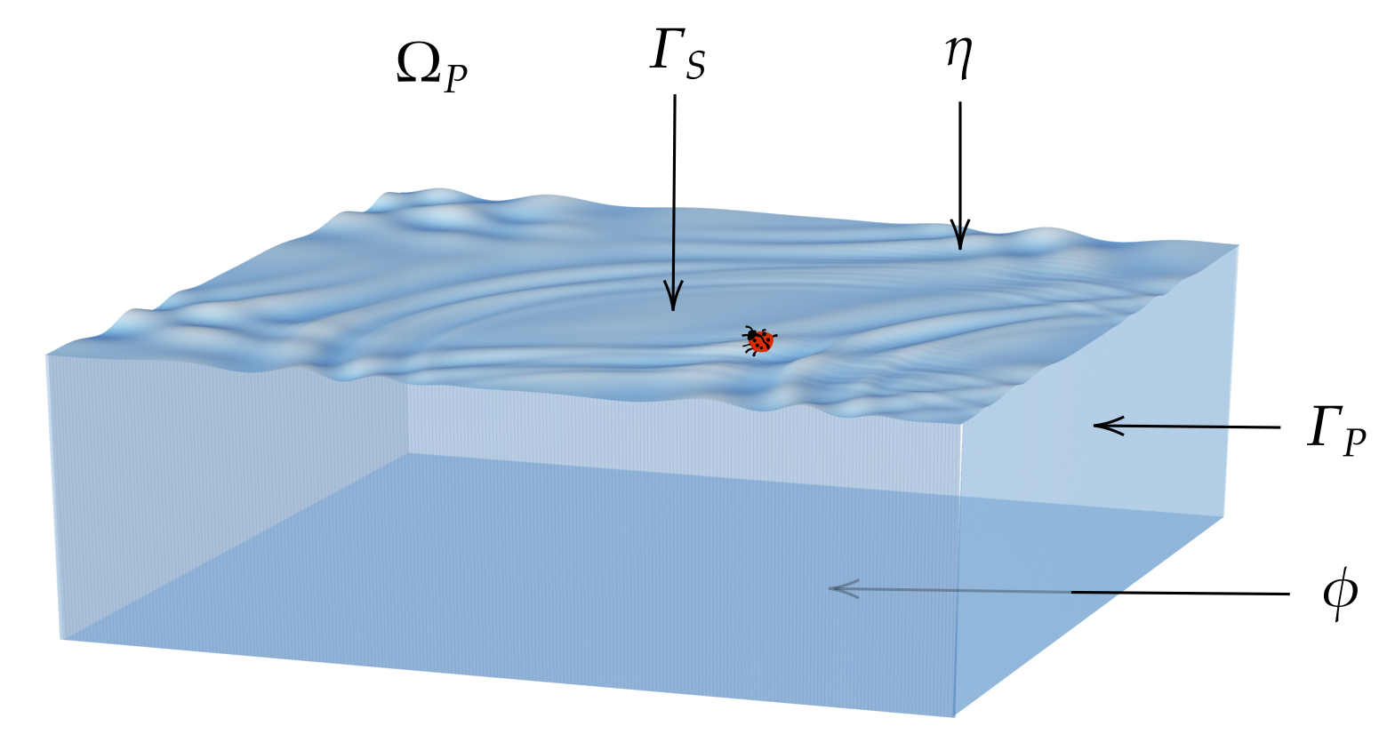
Figure 1: The domain $\Omega_{P}$. The surface wave amplitude $\eta$ lives on $\Gamma_{S}$, while $\phi$ is defined in all of $\Omega_{P}$, with homogeneous Neumann condition on the submerged pool boundary $\Gamma_{P}$. Is it possible for the ladybug to figure out the inital configuration of this seemingly chaotic wave field?

We model the disturbance of the initially calm water, the ”lots of people who have dived in the pool”, as the initial condition for the surface wave amplitude denoted by $\eta_{0}$, together with initial condition for the velocity potential $\phi$ at the surface, denoted $\varphi_{0}$. The model we consider is a linearized wave model with surface tension, the so-called Airy wave model. A derivation of this model together with a discussion of its validity can be found in, e.g., Ch. 5 in [1]. The small parameter in the linearization is the wave steepness $s=ka$, where $k$ is the wave number and $a$ is the maximum amplitude, and the linearization is known to be a good approximation when $s\ll 1$ (cf. Ch. 1 in [17] and references therein). The system of PDEs is

$$\begin{cases}\partial_{t}\eta-\partial_{z}\phi\big{|}_{z=0}=0,\quad X\in\Gamma_{S},t>0,\\ \partial_{t}\phi\big{|}_{z=0}+g\eta-S\Delta_{X}\eta=0,\quad X\in\Gamma_{S},t>0,\\ \Delta_{X,z}\phi=0,\quad(X,z)\in\Omega_{P},t>0,\\ \partial_{\nu}\phi=0,\quad(X,z)\in\Gamma_{P},t>0,\\ \partial_{\nu}\eta=0,\quad X\in\partial\Gamma_{S},t>0,\\ \left(\eta\big{|}_{t=0},\phi\big{|}_{z=0,t=0}\right)=\left(\eta_{0},\varphi_{0}\right),\quad X\in\Gamma_{S}.\end{cases}$$ (1)

Above, $g$ is the gravitational acceleration and $S=\frac{\sigma}{\rho}$, where $\sigma$ is the surface tension coefficient and $\rho$ is the mass density of water.

In (1), the first equation says that the velocity of the surface amplitude should equal the velocity of the water at the surface, while the second equation results from a linearization of the dynamic Bernoulli equation at the surface, and $\Delta_{X,z}\Phi=0$ is the incompressibility condition. The boundary condition on $\eta$ ensures that the waves are reflected at the edges of the pool, and the last equation is the initial condition.

2.2 Measurements

We will consider several different measurements. Let $\Gamma_{M}\subset\Gamma_{S}$ be some subset of the surface and for $0\leq t_{0}<t_{1}$, let $I_{T}=[t_{0},t_{1}]$ be the measurement time interval. In the analysis of the inverse problem for Feynman’s insect, we consider the measurement $\mathcal{M}$ to be

$$\mathcal{M}(X,t)=(\eta(X,t),\nabla_{X}\phi(X,0,t),\quad X\in\Gamma_{M},\quad t\in I_{T}.$$

That is, we assume we can measure the wave amplitude $\eta$ and horizontal water velocity $(V_{1},V_{2})=\nabla_{X}\phi(X,0,t)$ on the set $\Gamma_{M}$, i.e., the ”the irregularities and bumping of the waves” observed by the insect on the surface. In sections 4.2 and 4.3 we will assume that we only measure the amplitude, and consider noisy measurements, measurements of the wave velocity and discrete measurements.

3 Analysis of the water waves equation

Although linear water waves have been analysed by many before (cf. [14, 8, 17, 10, 1]), we were not able to find a complete analysis applicable to the initial-boundary value problem (1), and we therefore present it here.

3.1 Preliminaries

We can simplify equation (1) by considering the trace of the velocity potential at the surface. Let $\varphi(X,t)=\phi(X,z,t)|_{z=0}$. To reduce (1) to an equation for $(\eta,\varphi)$, we introduce the Dirichlet-to-Neumann (DN) operator $\mathcal{G}$,

$$\mathcal{G}\varphi=\partial_{z}\phi|_{z=0},\quad\text{where}\quad\begin{cases}\Delta_{X,z}\phi=0,\quad\text{in}\quad\Omega_{P},\\ \partial_{\nu}\phi=0,\quad\text{on}\quad\Gamma_{P},\\ \phi\big{|}_{z=0}=\varphi,\quad\text{on}\quad\Gamma_{S}.\end{cases}$$ (2)

Furthermore, we write $\mathcal{L}=(S\Delta_{X}-g)$. Formally, we can now write (1) as

$$\frac{\mathrm{d}}{\mathrm{d}t}\begin{pmatrix}\eta\\ \varphi\end{pmatrix}=\begin{bmatrix}0&\mathcal{G}\\ \mathcal{L}&0\end{bmatrix}\begin{pmatrix}\eta\\ \varphi\end{pmatrix},\quad\begin{pmatrix}\eta\\ \varphi\end{pmatrix}_{t=0}=\begin{pmatrix}\eta_{0}\\ \varphi_{0}\end{pmatrix}.$$ (3)

This is known as the Craig/Sulem–Zakharov formulation (cf. [18]), and it reduces the 2D-3D-system (1) to a 2D-2D-system for $(\eta,\varphi)$, at the expense of introducing the non-local DN operator.

To show well-posedness of (3), we follow the approch in [23] and apply semigroup theory. We first introduce some function spaces and show some properties of the operators $\mathcal{G}$ and $\mathcal{L}$.

First, note that for conservation of mass to hold in the pool, we must have $\text{vol}(\Omega_{P})=\int_{\Gamma_{S}}(H+\eta(X,t))\mathrm{d}X$ and hence $\int_{\Gamma_{S}}\eta(X,t)\mathrm{d}X=0,\forall t\geq 0.$ This motivates the use of the function space

$$\dot{L}^{2}=\left\{u\in L^{2}(\Gamma_{S}):\int_{\Gamma_{S}}u\mathrm{d}X=0\right\},$$

equipped with the $L^{2}$-inner product. Note that ${L^{2}(\Gamma_{S})=\{\text{constant functions}\}\cup\dot{L}^{2}(\Gamma_{S})}$, and so $\dot{L}^{2}$ is a Hilbert space. Moreover, the functions

$$\psi_{m,n}(X)=C_{m,n}\cos(\pi mx_{1}/L)\cos(\pi nx_{2}/W),\hskip 4.5ptC_{m,n}=\begin{cases}\frac{\sqrt{2}}{\sqrt{LW}},\quad\text{if }m\text{ or }n=0,\\ \frac{2}{\sqrt{LW}},\quad\text{else, }\end{cases}\hskip 4.5pt$$

with $m,n\in\mathbb{N}_{0},$ will be off use, and one can check that $\{\psi_{m,n}\}_{m+n>0}$ is an orthonormal basis for $\dot{L^{2}}$. We write $\hat{u}_{m,n}=(u,\psi_{m,n})_{L^{2}}$, and so $u\in\dot{L}^{2}$ has the expansion $u=\sum\psi_{m,n}\hat{u}_{m,n}.$ We also introduce the Sobolev spaces $\dot{H}^{s}$:

$$\dot{H}^{s}=\left\{u\in\dot{L}^{2}:\sum_{m+n>0}(m^{2}+n^{2})^{s}|\hat{u}_{m,n}|^{2}<\infty\right\},\quad s\in\mathbb{R}.$$

with the inner product $(u,v)_{\dot{H}^{s}}=\sum_{m+n>0}(m^{2}+n^{2})^{s}\hat{u}_{m,n}\hat{v}_{m,n}.$

3.2 The operators $\mathcal{G}$ and $\mathcal{L}$

We first consider the Dirichlet-to-Neumann operator. This operator is central in another inverse problem known as Electrical Impedance Tomography. Here one attempts to reconstruct the electrical conductivity in the interior of an object by applying a voltage to the boundary and measuring the resulting boundary current [21]. We now show that $\mathcal{G}$ from (2) is a self-adjoint and invertible operator from $\dot{H}^{1/2}$ to $\dot{H}^{-1/2}$.

Due to the simple geometry of the domain, we apply separation of variables to find that the solution to (2) is

$$\phi(X,z)=\sum_{m+n>0}\psi_{m,n}(X)\frac{\cosh(k_{m,n}(z+H))}{\sinh(k_{m,n}H)}\tanh(k_{m,n}H)(\varphi,\psi_{m,n})_{L^{2}(\Gamma_{S})},$$

where $k_{m,n}=\pi\sqrt{(m/L)^{2}+(n/W)^{2}}$. Hence

$$\mathcal{G}\varphi=\frac{\partial}{\partial z}\phi|_{z=0}=\sum_{m+n>0}k_{m,n}\tanh(k_{m,n}H)(\varphi,\psi_{m,n})_{L^{2}(\Gamma_{S})}\psi_{m,n}(X),$$

and we have expressed $\mathcal{G}$ in terms of the Fourier multiplier $|D|\tanh(|D|H)$. Injectivity of $\mathcal{G}$ follows by considering $\phi\in H^{2}(\Omega_{P})$ solution to (2) with Dirichlet data $\varphi\in\dot{H}^{1/2}$, and taking $\psi\in H^{1}(\Omega_{P})$. Integrating by parts, we have

$$-\int_{\Omega_{P}}\Delta_{X,z}\phi\psi\mathrm{d}V=\int_{\Omega_{P}}\nabla_{X,z}\phi\cdot\nabla_{X,z}\psi\mathrm{d}V-\int_{\Gamma_{S}}\partial_{z}\phi\psi\mathrm{d}X.$$ (4)

The requirement $\int\varphi\mathrm{d}X=0$ ensures uniqueness of $\mathcal{G}\varphi$: Assume $\mathcal{G}\varphi_{1}=\mathcal{G}\varphi_{2}$ for some $\varphi_{1}\neq\varphi_{2}$. With $\phi$ and $\psi$ solutions of (4) with boundary data $\varphi_{1}-\varphi_{2}$, we get that $\int_{\Omega_{P}}|\nabla_{X,z}\phi|^{2}\mathrm{d}V=0$, and hence $\phi=C$ for some constant $C$. But since $\int_{\Gamma_{S}}\phi|_{z=0}\mathrm{d}X=0$ we must have $C=0$ and so $\varphi_{1}=\varphi_{2}$. Moreover, for $\varphi_{1},\varphi_{2}\in\dot{H}^{1/2}$ and corresponding solutions $\phi,\psi$ of (2), we have

$$\int_{\Gamma_{S}}\partial_{z}\varphi_{1}\varphi_{2}\mathrm{d}X=\int_{\Omega_{P}}\nabla_{X,z}\phi\cdot\nabla_{X,z}\psi\mathrm{d}V=\int_{\Gamma_{S}}\varphi_{1}\partial_{z}\varphi_{2}\mathrm{d}X,$$

and so $\mathcal{G}$ is self-adjoint. Additionally, since we can find constants $a_{1},a_{2}>0$ such that

$$a_{1}|m^{2}+n^{2}|^{1/2}\leq k_{m,n}\tanh(k_{m,n}H)\leq a_{2}|m^{2}+n^{2}|^{1/2},$$

we infer that $\mathcal{G}:\dot{H}^{s}\to\dot{H}^{s-1}$, that $\mathcal{G}$ is invertible and that $(\mathcal{G}u,v)_{L^{2}}$ is an inner product on $\dot{H}^{1/2}$. We end with a physical observation: From (4) we get $(\mathcal{G}\varphi,\varphi)_{L^{2}}=\int_{\Omega_{P}}|\nabla_{X,z}\phi|^{2}\mathrm{d}X\geq 0$. Since $\nabla_{X,z}\phi=V$ is the velocity of the water, the latter integral is proportional to the kinetic energy $E_{k}$ of the water in the pool, since $E_{k}=\rho\int_{\Omega_{P}}V^{2}\mathrm{d}V.$

The boundary value problem associated with $\mathcal{L}$ (and $\eta$) is

$$\begin{cases}\mathcal{L}u=f,\quad\text{in}\quad\Gamma_{S},\\ \partial_{\nu}u=0\quad\text{on}\quad\partial\Gamma_{S}.\end{cases}$$

It has a unique solution $u\in\dot{H}^{1}$ for every $f\in\dot{L}^{2}$, and $u$ satisfies

$$(\mathcal{L}u,v)_{L^{2}}=S(\nabla u,\nabla v)_{L^{2}}+g(u,v)_{L^{2}}=-(f,v)_{L^{2}},\forall v\in\dot{H}^{1}.$$

Moreover, $\mathcal{L}$ is self-adjoint on $\dot{H}^{1}$ (cf. Ch. 8 in [26] for details), and it is a light calculation to check that

$$\mathcal{L}\psi_{m,n}=-(g+Sk_{m,n}^{2})\psi_{m,n},\quad m,n\in\mathbb{N}_{0}.$$

Consequently

$$u=\mathcal{L}^{-1}f=\sum_{m+n>0}\frac{\hat{f}_{m,n}}{-(g+Sk_{m,n}^{2})}\psi_{m,n}.$$

3.3 Well-posedness of the waves in the pool

We now introduce the energy space $H_{E}$ for the system (3). We write

$$A=\begin{bmatrix}0&\mathcal{G}\\ \mathcal{L}&0\end{bmatrix}\quad\text{and}\quad U=\begin{bmatrix}\eta\\ \varphi\end{bmatrix},$$

and set $D(A)=\{H^{2}\cap\dot{H^{1}}\times\dot{H}^{3/2}\}$. Now, let $H_{E}=\dot{H}^{1}\times\dot{H}^{1/2}$, equipped with the inner product

$$\langle U,V\rangle_{E} =S(\nabla u_{1},\nabla v_{1})_{L^{2}}+g(u_{1},v_{1})_{L^{2}}+(\mathcal{G}u_{2},v_{2})_{L^{2}},\quad U=\begin{pmatrix}u_{1}\\ u_{2}\end{pmatrix},V=\begin{pmatrix}v_{1}\\ v_{2}\end{pmatrix}\in H_{E}.$$

The $H_{E}$ norm is indeed a physical energy norm: the term $S(\nabla\eta,\nabla\eta)_{L^{2}}$ represents the elastic energy due to the surface tension and the terms $g(\eta,\eta)_{L^{2}}$ and $(\mathcal{G}\varphi,\varphi)_{L^{2}}$ are proportional to the potential and kinetic energy of the water, respectively. Next, note that

$$\langle U,V\rangle_{E} =S(\nabla u_{1},\nabla v_{1})_{L^{2}}+g(u_{1},v_{1})_{L^{2}}+(\mathcal{G}u_{2},v_{2})_{L^{2}}$$

$$=-(u_{1},\mathcal{L}v_{1})_{L^{2}}+(u_{2},\mathcal{G}v_{2})_{L^{2}},\quad U=\begin{pmatrix}u_{1}\\ u_{2}\end{pmatrix},V=\begin{pmatrix}v_{1}\\ v_{2}\end{pmatrix}\in D(A).$$

Since $\dot{U}=AU$, we now see that $\|U\|_{E}^{2}=\langle U,U\rangle_{E}^{2}$ is conserved: Assuming $U$ solves (3), we have

$$\frac{\mathrm{d}}{\mathrm{d}t}\left(\frac{1}{2}\|U\|_{E}^{2}\right)=\langle\dot{U},U\rangle_{E}=-(\mathcal{G}u_{2},\mathcal{L}u_{1})_{L^{2}}+(\mathcal{L}u_{1},\mathcal{G}u_{2})_{L^{2}}=0.$$

We are now in a position to show well-posedness of (3).

Theorem 1.

For each $U_{0}=(\eta_{0},\varphi_{0})\in H_{E}$, the water waves system (3) has a unique solution $U=(\eta,\varphi)^{T}\in C([0,\infty);H_{E}).$ The solution is given by

$$\begin{split}U(t)&=\sum_{m,n\geq 0}\cos(\omega_{m,n}t)\psi_{m,n}\begin{bmatrix}(\eta_{0},\psi_{m,n})_{L^{2}}\vspace{3mm}\\ (\varphi_{0},\psi_{m,n})_{L^{2}}\end{bmatrix}\\ &+\sin(\omega_{m,n}t)\psi_{m,n}\begin{bmatrix}\frac{\omega_{m,n}}{g+Sk^{2}_{m,n}}(\varphi_{0},\psi_{m,n})_{L^{2}}\vspace{3mm}\\ -\frac{g+Sk_{m,n}^{2}}{\omega_{m,n}}(\eta_{0},\psi_{m,n})_{L^{2}}\end{bmatrix},\end{split}$$ (5)

and satisfies $\|U(t)\|_{E}=\|U_{0}\|_{E}$ for all $t$. Above

$$\omega_{m,n}=\sqrt{(gk_{m,n}+Sk_{m,n}^{3})\tanh(k_{m,n}H)})$$ (6)

is the dispersion relation for gravity-capillary waves. Moreover, for $(\eta_{0},\varphi_{0})\in\dot{H}^{s+\frac{1}{2}}\times\dot{H}^{s}$ with $s\geq 1/2,$ we have that

$$\eta\in\dot{H}^{s+\frac{1}{2}}\quad\text{and}\quad\varphi\in\dot{H}^{s}\quad\text{for all }t\geq 0.$$

Note: To ease notation later, the sum above includes $(m,n)=(0,0)$, although the term is always zero since $(\psi_{0,0},f)_{L^{2}}=0$ for $f\in\dot{L}^{2}$.

Proof.

We first show that $A:D(A)\to H_{E}$ is skew-adjoint. One readily verifies that $A$ is skew-symmetric:

$$\langle AU,V\rangle_{E}=-\langle U,AV\rangle_{E},\quad\forall U,V\in D(A).$$

If in addition $R(A)=H_{E}$, where $R(A)$ denotes the range of $A$, we can conclude that $A$ is skew-adjoint (cf. Ch. 3.7 in [33]). But this is immediate, since both $\mathcal{L}$ and $\mathcal{G}$ are invertible and we have

$$A^{-1}=\begin{bmatrix}0&\mathcal{L}^{-1}\\ \mathcal{G}^{-1}&0\end{bmatrix}.$$

Since $A$ is skew-adjoint, it is the generator of a strongly continuous, unitary semigroup $\mathbb{T}_{t}$ (cf. Thm. 3.8.6, [33]). Hence the unique solution to the initial value problem $\dot{z}=Az,z(0)=z_{0}$ in (3) is given by $z(t)=\mathbb{T}_{t}z_{0}$, and $z\in C([0,\infty);H_{E})$ satisfies $\|z(t)\|_{E}=\|z_{0}\|_{E}$.

Moreover, $A$ is diagonizable. Indeed, one can check that

$$AV_{m,n}^{\pm}=\pm i\omega_{m,n}V_{m,n}^{\pm},$$

where

$$V_{m,n}^{\pm}=\begin{bmatrix}(2(g+Sk_{m,n}^{2}))^{-1/2}\vspace{3mm}\\ \pm i(2k_{m,n}\tanh(k_{m,n}H))^{-1/2}\end{bmatrix}\psi_{m,n}\quad\text{and}\quad\omega_{m,n}=\sqrt{(gk_{m,n}+Sk_{m,n}^{3})\tanh(k_{m,n}H)}.$$

The eigenvectors here are chosen such that $\{V^{+}_{m,n}\}$ and $\{V^{-}_{m,n}\}$ are biorthogonal sequences, i.e., $\langle V_{m,n}^{+},V_{i,j}^{-}\rangle_{E}=\delta_{m,n,i,j}.$ Consequently,

$$U(t)=\sum_{m,n\geq 0}e^{i\omega_{m,n}t}\langle U_{0},V^{-}_{m,n}\rangle_{E}V_{m,n}^{+}+e^{-i\omega_{m,n}t}\langle U_{0},V^{+}_{m,n}\rangle_{E}V^{-}_{m,n}.$$

Since

$$e^{i\omega_{m,n}t}\langle U_{0},V^{-}_{m,n}\rangle_{E}V_{m,n}^{+}+e^{-i\omega_{m,n}t}\langle U_{0},V^{-}_{m,n}\rangle_{E}V^{+}_{m,n}=2\text{Re}(e^{i\omega_{m,n}t}\langle U_{0},V^{-}_{m,n}\rangle_{E}V^{+}_{m,n}),$$

and

$$\langle U_{0},V^{-}_{m,n}\rangle_{E}V_{m,n}^{+}=\frac{1}{2}\begin{bmatrix}(\eta_{0},\psi_{m,n})_{L^{2}}-i\frac{(k_{m,n}\tanh(k_{m,n}H))^{1/2}}{(g+Sk_{m,n}^{2})^{1/2}}(\varphi_{0},\psi_{m,n})_{L^{2}}\vspace{3mm}\\ (\varphi_{0},\psi_{m,n})_{L^{2}}+i\frac{(g+Sk_{m,n}^{2})^{1/2}}{(k_{m,n}\tanh(k_{m,n}H))^{1/2}}(\eta_{0},\psi_{m,n})_{L^{2}}\end{bmatrix}\psi_{m,n},$$

it follows that

$$U(t)=\sum_{m,n\geq 0}\cos(\omega_{m,n}t)\psi_{m,n}\begin{bmatrix}(\eta_{0},\psi_{m,n})_{L^{2}}\vspace{3mm}\\ (\varphi_{0},\psi_{m,n})_{L^{2}}\end{bmatrix}+\sin(\omega_{m,n}t)\psi_{m,n}\begin{bmatrix}\frac{\omega_{m,n}}{g+Sk^{2}_{m,n}}(\varphi_{0},\psi_{m,n})_{L^{2}}\vspace{3mm}\\ -\frac{g+Sk_{m,n}^{2}}{\omega_{m,n}}(\eta_{0},\psi_{m,n})_{L^{2}}\end{bmatrix}.$$

Last, note that for $m+n>0$, we can find positive constants such that

$$\begin{split}c_{1}|m^{2}+n^{2}|^{-1/4}&\leq\frac{\omega_{m,n}}{g+Sk^{2}_{m,n}}\leq c_{2}|m^{2}+n^{2}|^{-1/4},\\ \tilde{c}_{1}|m^{2}+n^{2}|^{1/4}&\leq\frac{g+Sk_{m,n}^{2}}{\omega_{m,n}}\leq\tilde{c}_{2}|m^{2}+n^{2}|^{1/4}.\end{split}$$

Assuming $(\eta_{0},\varphi_{0})\in\dot{H}^{s+\frac{1}{2}}\times\dot{H}^{s}$, we see that

$$\|\eta(X,t)\|_{\dot{H}^{s+\frac{1}{2}}} \leq\|\eta_{0}\|_{\dot{H}^{s+\frac{1}{2}}}+\left\|\sum_{m,n}\frac{\omega_{m,n}}{g+Sk^{2}_{m,n}}(\varphi_{0},\psi_{m,n})_{L^{2}}\psi_{m,n}\right\|_{\dot{H}^{s+\frac{1}{2}}}$$

$$\leq C\left(\|\eta_{0}\|_{\dot{H}^{s+\frac{1}{2}}}+\|\varphi_{0}\|_{\dot{H}^{s}}\right),$$

$$\|\varphi(X,t)\|_{\dot{H}^{s}} \leq\|\varphi_{0}\|_{\dot{H}^{s}}+\left\|\sum_{m,n}\frac{g+Sk^{2}_{m,n}}{\omega_{m,n}}(\eta_{0},\psi_{m,n})_{L^{2}}\psi_{m,n}\right\|_{\dot{H}^{s}}$$

$$\leq\tilde{C}\left(\|\varphi_{0}\|_{\dot{H}^{s}}+\|\varphi_{0}\|_{\dot{H}^{s+\frac{1}{2}}}\right).$$

∎

With the well-posedness of the forward problems established, we are ready to tackle the inverse problem.

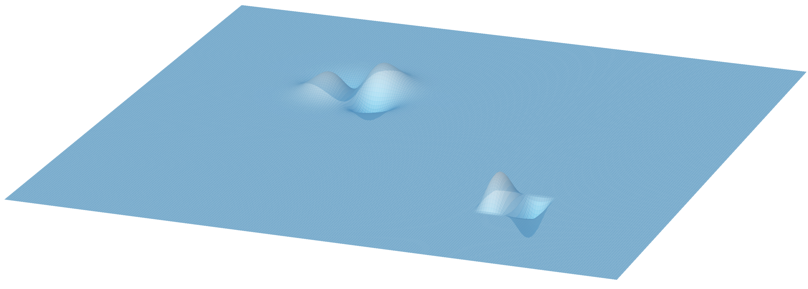
(a) $t=0$

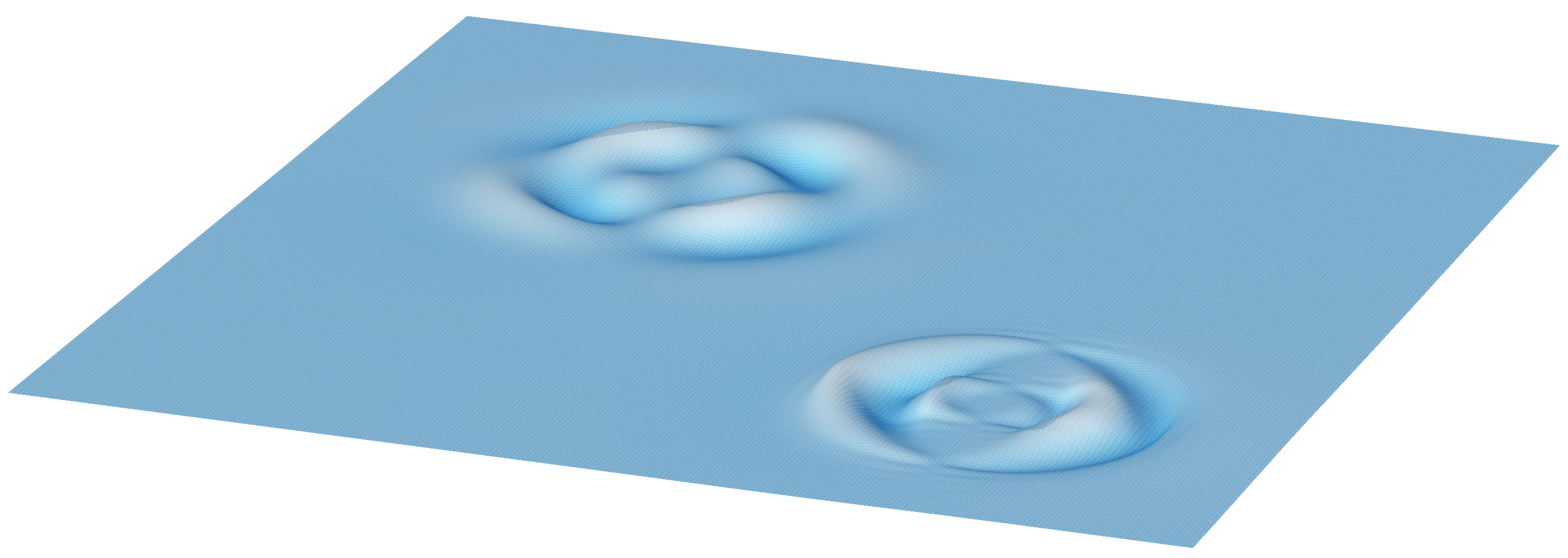
(b) $t=0.5$

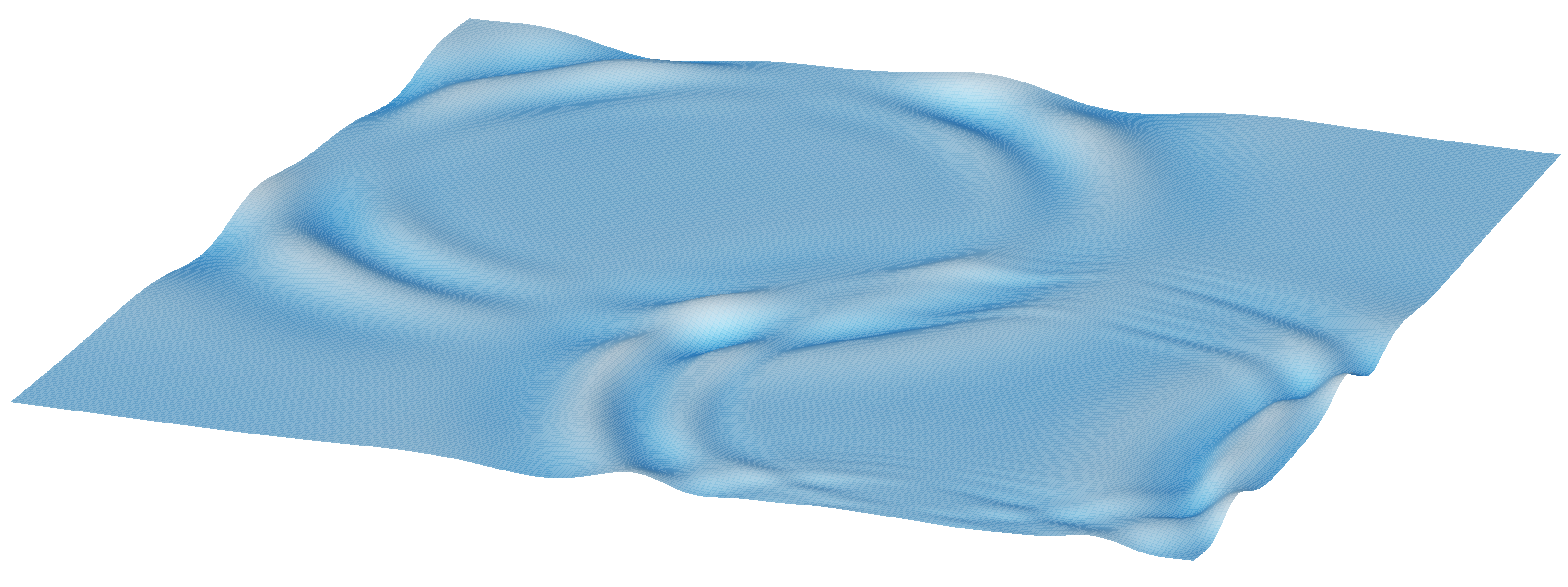
(c) $t=1.5$

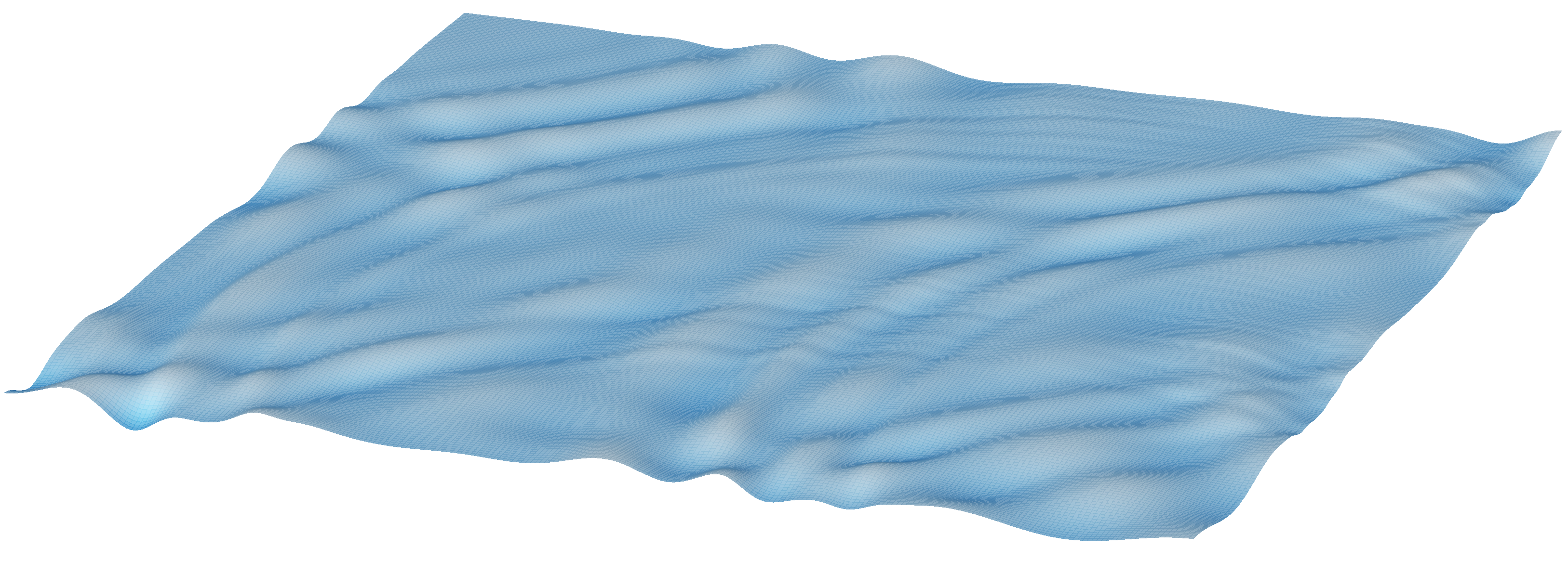
(d) $t=3.5$

Figure 2: The figure shows four snapshots of the wave amplitude $\eta$, with the initial condition and pool parameteres as given in Section 5.2.

4 The inverse problem

We now analyse the inverse problem for several different measurement scenarios. We consider the following problems:

• Unique determination of the initial disturbance from measurement on a small domain.

• Stability of reconstructing the initial disturbance from measurements along the side of the pool.

• Stability of reconstruction of from discrete measurements.

4.1 Problem 1: Unique determination of the initial disturbance for Feynman’s clever insect

Assume the domain $\Gamma_{M}$ is a non-empty, open subset of the surface $\Gamma_{S}$, and let $I_{T}=[t_{0},t_{1}]$ be the measurement time interval. Let the measurement be $\mathcal{M}(X,t)=(\eta(X,t),\nabla_{X}\varphi(X,t))$ with $(X,t)\in\Gamma_{M}\times I_{T}$.

Theorem 2.

Assume $(\eta_{0},\varphi_{0})\in\dot{H}^{\frac{3}{2}}\times\dot{H}^{1}$. Then the measurement $\mathcal{M}(X,t)$ uniquely determines the initial disturbance $(\eta_{0},\varphi_{0})$.

Remark 1.

The above result might seem strange at first, as this type of result is not true for many other type of waves, e.g., acoustic and electromagnetic waves. Consider for example the Cauchy problem for the wave equation in $\mathbb{R}^{n}$,

$$(\partial_{t}^{2}-\Delta)u=0,\quad(u(0),\partial_{t}u(0))=(u_{0},u_{1}).$$

Then Huygens’ principle says that if for some ball $B_{R}(0)$ with radius $R$ we have that $\text{supp}(u_{0})\cup\text{supp}(u_{1})\subset B_{R}(0)$, then $\text{supp}(u(t,x))\subset B_{R+t}$ for all $t\geq 0$ (cf. Ch 6 in [11]). The propagation speed is finite and the wavefront of a compactly supported source $u_{0}$ will propagate as ${u_{0}(x-ct)}$, and hence not be detectable on arbitrary space-time domains $\Gamma_{M}\times I_{T}$ (cf. [30]). The result also has the bizarre consequence that if the water is still on some open set on the surface for a tiny duration of time, then the the whole body of water must have been still everywhere and for all time. As becomes clear in the proof, it is the non-local behaviour of the DN operator that is the mechanism enabling this property; due to the modeling of the fluid as incompressible and irrotational, the velcoity potential is harmonic. This allows for the application of unqiue continuation, but it is still suprising that this property propagates enough information to ensure uniqueness for the surface wave. However, for the Schrödinger equation, which is also a dispersive PDE, results like the above are known to hold (cf. [32]). Moreover, there has recently been much interest in inverse problems related to fractional PDEs (cf. [25, 15]). Fractional differential operators are also non-local operators, and, e.g., in [9] the authors prove unqiue continuation for an inverse problem in fractional elasticity.

Proof.

The proof relies on the following unique continuation result from [2]: Let $\Omega$ be a convex domain and assume $\Delta u=0$ in $\Omega$. Let $\Gamma\subset\partial\Omega$ be a subset of the boundary with positive surface measure. Then $u|_{\Gamma}=\partial_{\nu}u|_{\Gamma}=0$ implies that $u=0\text{ in }\Omega$.

By Theorem 1, the measurement is well-defined in the sense that $\int_{\Gamma_{S}}\mathcal{M}h\mathrm{d}X$ is bounded for all $h\in C^{\infty}(\Gamma_{S})$. Now, assume $\mathcal{M}(X,t)=0$ for $(X,t)\in\Gamma_{M}\times I_{T}$. Then $\dot{\eta}=0$ in some space-time cylinder $Q_{\varepsilon}=B_{\epsilon}\times I_{\varepsilon}\subset\Gamma_{M}\times I_{T}$, and by (3) this implies that $\mathcal{G}\varphi=0$ and $\dot{\varphi}=0$ in $Q_{\varepsilon}$. Moreover, since $\nabla_{X}\varphi=0$ in $Q_{\varepsilon}$, we must have $\varphi|_{Q_{\varepsilon}}=C_{\varepsilon}$ for some constant $C_{\varepsilon}$. But this implies $\phi=C_{\varepsilon}$: Assume there is some $\tilde{\phi}\neq C_{\varepsilon}$, and such that $\tilde{\phi}|_{Q_{\varepsilon}}=C_{\varepsilon}$ and $\partial_{z}\tilde{\phi}|_{Q_{\varepsilon}}=0$. Then $\tilde{\phi}-C_{\varepsilon}$ is harmonic in $\Omega_{P}$ and satisfies ${(\tilde{\phi}-C_{\varepsilon})|_{Q_{\varepsilon}}=\partial_{z}(\tilde{\phi}-C_{\varepsilon})|_{Q_{\varepsilon}}=0}$. Since $\Omega_{P}$ is convex, we can apply the unique continuation result and conclude that $\tilde{\phi}=C_{\varepsilon}$ in $\Omega_{P}$. Therefore $\varphi=C_{\varepsilon}$, and since $\varphi\in\dot{L}^{2}$, $\varphi=0$. Hence, with $\dot{\varphi}=0$, we have that $(S\Delta_{X}-g)\eta=0$ on $\Gamma_{S}$. But since $g/S>0$, the only solution to $-\Delta_{X}\eta=-\frac{g}{S}\eta$ on $\Gamma_{S}$ with homogeneous Neumann conditions is $\eta=0$. By Theorem 1 we have $\|(\eta(X,t),\varphi(X,t))\|_{E}=\|(\eta_{0},\varphi_{0})\|_{E}$ for all $t\geq 0$ and hence $(\eta_{0},\varphi_{0})=0$, and since the map $(\eta_{0},\varphi_{0})\mapsto\mathcal{M}$ is linear, the conclusion now follows. ∎

For waves in the linear regime, the answer to Feynman’s question is therefore positive:

Corollary 1.

A sufficiently clever insect can determine the initial disturbance in the pool.

However, the above result is based on a unique continuation argument, it says nothing about the stability of the procedure of inversion. In fact, unique continuation is known to be a severely ill-posed problem [12]. Hence, an observer not sufficiently clever that makes imperfect measurements would very likely not succeed with the task of computing the initial conditions. In the next section we investigate the stability properties of the inverse problem.

4.2 Problem 2: Uniqueness and stability from measurements along two adjacent sides of the pool

From the study of the observability of wave equations, it is well known that the part of the boundary where one measures the wave should satisfy certain geometric conditions. Typically, one relies on microlocal analysis or the multiplier method for to show this (cf. [7, 33]), but we have not found these methods suitable for our problem. Instead, we utilize the explicit solution in Theorem 1 and a so-called spectral observability method used in, e.g., [32, 16, 33]. We assume now that we measure the wave amplitude along two adjacent sides of the pool, i.e.,

$$\mathcal{M}(X,t)=\eta(X,t)|_{X\in\Gamma_{M}},\quad\text{with }\Gamma_{M}=\left\{(x_{1},0):x_{1}\in(0,L)\right\}\cup\left\{(0,x_{2}):x_{2}\in(0,W)\right\}.$$

We then obtain the following result:

Theorem 3.

Assume the measurement time satisfies

$$T\geq\frac{6L\sqrt{L^{2}+W^{2}}}{W}\left(\frac{Hg}{2\sqrt{1+\frac{H^{2}g}{3S}}}-\frac{3S}{2H}\right)^{-1/2}.$$ (7)

Then there is a constant $C$, independent of $(\eta_{0},\varphi_{0})$, such that following stability estimate holds

$$\int_{0}^{T}\int_{\Gamma_{M}}|\mathcal{M}(X,t)|^{2}\mathrm{d}X\mathrm{d}t\geq CT\left(\|\eta_{0}\|_{L^{2}}^{2}+\|\varphi_{0}\|_{\dot{H}^{-\frac{1}{2}}}^{2}\right).$$ (8)

Remark 2.

In the above estimate, the term

$$\tiny{\left(\frac{Hg}{2\sqrt{1+\frac{H^{2}g}{3S}}}-\frac{3S}{2H}\right)^{-1/2}}$$

is a lower bound on the group velocity $c_{g}=\partial_{k}\omega(k)$ of the water waves. The group velocity is the velocity with which a localized wave group/wavelet propagates, and it is also the velocity of the energy transport (cf. [1]). The lower bound on the observation time $T$ is given by a term proportional to the maximal length of the pool times the minimal group velocity. This is comparable to similar bounds for acoustic or electromagnetic waves, where the bound is proportional to the the minimal wave velocity times the maximal distance (cf. [4]). Moreover, as we will see in the proof of Theorem 8, the presence of capillary waves is necessary to have stability. In fact, for pure gravitational waves ($S=0$ in (6)), the group speed $c_{g}(k)=\partial_{k}\omega(k)\sim k^{-1/2}$ approaches zero as the wavenumber $k$ increases. Consequently, one can for any $T>0$ imagine a compactly supported source comprised of modes with frequencies so high that they do not reach the boundary during the measurement time $T$. In contrast, for gravity-capillary waves, this cannot happen, as $c_{g}(k)\sim k^{1/2}$.

The above result implies uniqueness, but more important, stability. If we have a noisy measurement $\tilde{\mathcal{M}}=\mathcal{M}+\varepsilon$, and we obtain from $\tilde{\mathcal{M}}$ a reconstruction $(\tilde{\eta}_{0},\tilde{\varphi}_{0})$ of $(\eta_{0},\varphi_{0})$, it shows that the reconstruction error (if the reconstruction is done correctly) is bounded by the measurement error, i.e.,

$$\int_{0}^{T}\int_{\Gamma_{M}}|\varepsilon|^{2}\mathrm{d}X\mathrm{d}t\geq C\frac{T}{L\pi}\left(\|\eta_{0}-\tilde{\eta}_{0}\|_{L^{2}}^{2}+\|\varphi_{0}-\tilde{\varphi}_{0}\|_{\dot{H}^{-\frac{1}{2}}}^{2}\right).$$

Additional stability

When analysing inverse problems, a rule-of-thumb is that the more precise measurement we are able to make, the more accurate our reconstruction should be. For example, if we can measure the amplitude with such precision that we can compute the (vertical) wave velocity without too much error, or if we are able to directly measure the velocity or acceleration, this information should result in a better reconstruction. We can quantify is by expressing the stability estimate in terms of stronger topologies, i.e., norms that include derivatives, and as simple consequence of Theorem 8, we get the following corollary.

Corollary 2.

Assume $k\in\mathbb{N}_{0}$, $(\eta_{0},\varphi_{0})\in\dot{H}^{\frac{3}{2}k}\times\dot{H}^{\frac{3}{2}k-\frac{1}{2}}$, and that $T$ satisfies the same bound as in Theorem 8. Then there is a constant $C_{k}$, independent of $(\eta_{0},\varphi_{0})$, such that following stability estimate holds

$$\int_{0}^{T}\int_{\Gamma_{M}}|\partial_{t}^{k}\eta(X,t)|^{2}\mathrm{d}X\mathrm{d}t\geq C_{k}T(\|\eta_{0}\|_{\dot{H}^{\frac{3}{2}k}}^{2}+\|\varphi_{0}\|_{\dot{H}^{\frac{3}{2}k-\frac{1}{2}}}^{2}).$$ (9)

Theorem 8 relies on some results from non-harmonic Fourier analysis.

Measurements and non-harmonic Fourier series

The measurement operator takes the form

$$\mathcal{M}(X,t)=\sum_{m,n\geq 0}^{\infty}\psi_{m,n}(X)\left(\cos(\omega_{m,n}t)q_{m,n}+\sin(\omega_{m,n}t)\frac{\omega_{m,n}}{g+Sk_{m,n}^{2}}p_{m,n}\right),$$ (10)

with and $q_{m,n}=(\eta_{0},\psi_{m,n})_{L^{2}(\Gamma_{S})}$ and $p_{m,n}=(\varphi_{0},\psi_{m,n})_{L^{2}(\Gamma_{S})}$. With

$$c_{m,n}=\frac{1}{2}\left(q_{m,n}-i\frac{\omega_{m,n}}{g+Sk_{m,n}^{2}}p_{m,n}\right)\quad\text{for}\quad m,n\geq 0,$$

we may now write

$$\mathcal{M}(X,t)=\sum_{m\geq 0}\left(\sum_{n\geq 0}^{\infty}\psi_{m,n}(X)c_{m,n}e^{i\omega_{m,n}t}+c.c.\right),$$

where $c.c.$ denotes the complex conjugate of $\sum_{n\geq 0}^{\infty}\psi_{m,n}(X)c_{m,n}e^{i\omega_{m,n}t}$. If we now fix $m$ and temporarily ignore the spatial dependence in the above expression, we have a function on the form

$$f_{m}(t)=\sum_{n\geq 0}c_{m,n}\mathrm{e}^{i\omega_{m,n}t}+c.c..$$ (11)

Such functions are called non-harmonic Fourier series (or almost periodic functions) [35, 33]. In general, they are functions on the form

$$f(t)=\sum_{n\in\mathbb{Z}}a_{n}\mathrm{e}^{i\lambda_{n}t},\quad(a_{n})\in\ell^{2},\lambda_{n}\in\Lambda,$$

where the frequency set $\Lambda=\{\lambda_{n}\}_{n\in\mathcal{I}}$ differs from the classical $\{2\pi n/T\}_{n\in\mathbb{Z}}$. When the frequency set is non-harmonic, as is the case with $\{\omega_{m,n}\}$, we cannot immediately apply Fourier inversion. But under certain conditions, we can get a result similar to Parseval’s identitiy; Ingham’s theorem (cf. [33]) states that if ${\inf_{m\neq n}|\lambda_{n}-\lambda_{m}|=\gamma>0}$ and $T>2\pi/\gamma$, then there are positive constants $c_{-},c_{+}$ such that

$$c_{-}\sum_{n}|a_{n}|^{2}\leq\int_{0}^{T}\big{|}\sum_{n}a_{n}e^{i\lambda_{n}t}\big{|}^{2}\mathrm{d}t\leq c_{+}\sum_{n}|a_{n}|^{2}.$$

For fixed $m$ (or $n$), the set $\{\omega_{m,n}\}_{n}$ satisfies the requirements of Ingham’s theorem, and we will use this is section 4.3. However, one can check that $|\omega_{m,0}-\omega_{m,1}|\to 0$ as $m\to\infty.$, i.e., if both indices are allowed to vary, the gap condition does not hold. To circumvent this, we will use the following, weaker version of Ingham’s theorem, invented in [19] and used to prove observability of the wave equation in [20, 16].

Theorem 4.

(Weakened Ingham’s Theorem)(Proposition 3.1 in [16]) Let $\{\lambda_{k}\}_{k\in\mathbb{Z}}$ be a sequence of real numbers and $N$ a positive integer, and assume there exists some $\gamma>0$ such that

$$|\lambda_{k}-\lambda_{l}|\geq|k-l|\gamma\quad\text{if}\quad\max(|k|,|l|)\geq N.$$

Then it holds for any $(a_{n})\in\ell^{2}$ and $T>0$ that

$$\int_{0}^{T}\big{|}\sum_{k\in\mathbb{Z}}a_{k}e^{i\lambda_{k}t}\big{|}^{2}\mathrm{d}t\geq\frac{2T}{\pi}\left(\sum_{|k|\geq N}|a_{k}|^{2}-\left(\frac{2\pi}{T\gamma}\right)^{2}\sum_{k\in\mathbb{Z}}|a_{k}|^{2}\right).$$ (12)

We now want to adapt the observability proof from [20, 16] to water waves. To show that Theorem 12 is satisfied for $f_{m}(t)$ in (11), we note that with

$$\lambda_{k}^{m}=\begin{cases}\text{sgn}(k)\omega_{m,|k|-1},\quad|k|>0,\\ 0,\quad k=0,\end{cases}\quad\text{and}\quad a_{k}^{m}=\begin{cases}c_{m,k-1},\quad k>0\\ \bar{c}_{m,|k|-1},\quad k<0,\\ 0,\quad k=0,\end{cases}\quad\text{for }k\in\mathbb{Z},$$

we have

$$\sum_{k\in\mathbb{Z}}a_{k}^{m}e^{i\lambda_{k}^{m}t}=f_{m}(t).$$

Hence, if the gap condition in Theorem 12 holds for the frequency set $\{\lambda_{k}^{m}\}_{k\in\mathbb{Z}}$, then (12) holds for $f_{m}(t)$.

Lemma 1.

For any $m,n\in\mathbb{N}_{0}$, let

$$\{\lambda_{k}^{m}=\text{sgn}(k)\omega_{m,|k|-1}\}_{k\in\mathbb{Z}}\quad\text{and}\quad\{\tilde{\lambda}_{k}^{n}=\text{sgn}(k)\omega_{|k|-1,n}\}_{k\in\mathbb{Z}}.$$

It then holds for $k,l\in\mathbb{Z}$ that

$$|\lambda_{k}^{m}-\lambda_{l}^{m}| \geq|k-l|\gamma,\quad\text{for }\max(|k|,|l|)\geq m,$$

$$|\tilde{\lambda}_{k}^{n}-\tilde{\lambda}_{l}^{n}| \geq|k-l|\gamma,\quad\text{for }\max(|k|,|l|)\geq n,$$

with

$$\gamma=\frac{\pi W}{2L\sqrt{L^{2}+W^{2}}}\sqrt{\frac{Hg}{2\sqrt{1+\frac{H^{2}g}{3S}}}-\frac{3S}{2H}}.$$

Proof.

If $\text{sgn}(k)=\text{sgn}(l)$, then $|\lambda^{m}_{k}-\lambda^{m}_{l}|=|\omega_{m,|k|-1}-\omega_{m,|l|-1}|$. On the other hand, for $k,l>0$

$$\lambda_{k}^{m}-\lambda_{-l}^{m}=\omega_{m,k-1}+\omega_{m,l-1}\geq\omega_{m,k-1}-\omega_{m,l-1},$$

and so if for any $p,q\geq 0$ it holds that

$$|\omega_{m,p}-\omega_{m,q}|\geq|p-q|\gamma\quad\text{and}\quad\omega_{m,p}\geq p\gamma\quad\text{for }\max(p,q)\geq m,$$

then the gap condition holds for $\{\lambda_{k}\}_{k\in\mathbb{Z}\setminus\{0\}}$.

Consider now the function $G(t)=\sqrt{(gt+St^{3})\tanh(tH)}$ for $t>0$. We have

$$G^{\prime}(t)=\frac{(g+3St^{2})\tanh(tH)+H(gt+St^{3})\text{sech}(tH)^{2}}{2\sqrt{(gt+St^{3})\tanh(tH)}}$$

Using elementary inequalities together with the lower bound $\tanh(t)>t/\sqrt{1+t^{2}},t>0,$ (see Lemma 4 in [6]), we find that

$$G^{\prime}(t)>\sqrt{\frac{H(g+3St^{2})}{4(1+Ht)}}\geq\sqrt{\frac{Hg}{2\sqrt{1+\frac{H^{2}g}{3S}}}-\frac{3S}{2H}}\tilde{\gamma}$$

Fixing $m$ and assuming $p\geq m$ and $p>q\geq 0$, we have that

$$k_{m,p}\leq\pi p\sqrt{L^{-2}+W^{-2}}<\pi(p+q)\sqrt{L^{-2}+W^{-2}}\quad\text{and}\quad k_{m,p}^{2}-k_{m,q}^{2}=\frac{\pi^{2}}{W^{2}}(p^{2}-q^{2}).$$

Hence

$$|k_{m,p}-k_{m,q}|=\frac{|k_{m,p}^{2}-k_{m,q}^{2}|}{|k_{m,p}+k_{m,q}|}>\frac{\frac{\pi^{2}}{W^{2}}|p-q||p+q|}{2\pi|p+q|\sqrt{L^{-2}+W^{-2}}}\geq\frac{\pi L}{2W\sqrt{L^{2}+W^{2}}}|p-q|.$$

We now get

$$\begin{split}|\omega_{m,p}-\omega_{m,q}|&=|G(k_{m,p})-G(k_{m,q})|\\ &=\bigg{|}\int_{k_{m,p}}^{k_{m,q}}G^{\prime}(t)\mathrm{d}t\bigg{|}\geq\frac{\pi L}{2W\sqrt{L^{2}+W^{2}}}|p-q|\tilde{\gamma}.\end{split}$$ (13)

We also have that $k_{m,p}\geq\frac{\pi}{W}p$ and so $\omega_{m,p}\geq\frac{\pi}{W}p\tilde{\gamma}$. By the same procedure we find the estimate

$$|\omega_{p,n}-\omega_{q,n}|\geq\frac{\pi W}{2L\sqrt{L^{2}+W^{2}}}|p-q|\tilde{\gamma},$$

and since we have assumed $L\geq W$, we get the result. ∎

We can now prove Theorem 8.

Proof.

On the boundary we have

$$\mathcal{M}(X,t)|_{x_{2}=0} =\sum_{m\geq 0}\frac{C_{m,|n|}}{\sqrt{WL}}\cos(\pi mx_{1}/L)\sum_{n\in\mathbb{Z}}a_{k}^{n}e^{i\lambda_{n}^{m}t},$$

$$\mathcal{M}(X,t)|_{x_{1}=0} =\sum_{n\geq 0}\frac{C_{|m|,n}}{\sqrt{WL}}\cos(\pi nx_{2}/L)\sum_{m\in\mathbb{Z}}b_{m}^{n}e^{i\tilde{\lambda}_{m}^{n}t},$$

where

$$b_{m}^{n}=\begin{cases}c_{m-1,n},\quad m>0\\ \bar{c}_{|m|-1,n},\quad km0,\\ 0,\quad m=0,\end{cases}\quad\text{for }k\in\mathbb{Z}.$$

We write

$$I_{1}=\int_{0}^{T}\int_{0}^{L}|\mathcal{M}(X,t)|^{2}\mathrm{d}x_{1}\mathrm{d}t\quad\text{and}\quad I_{2}=\int_{0}^{T}\int_{0}^{W}|\mathcal{M}(X,t)|^{2}\mathrm{d}x_{2}\mathrm{d}t,$$

and by orthogonality and Theorem 12 and Lemma 1, we now have

$$I_{1}=\frac{2}{W}\sum_{m\geq 0}\int_{0}^{T}\bigg{|}\sum_{n\in\mathbb{Z}}a_{n}^{m}e^{i\lambda_{n}^{m}t}\bigg{|}^{2}\mathrm{d}t\geq\frac{4T}{W\pi}\sum_{m\geq 0}\left(\sum_{\begin{subarray}{c}n\in\mathbb{Z}\\ |n|\geq m\end{subarray}}|a_{n}^{m}|^{2}-\left(\frac{2\pi}{T\gamma}\right)^{2}\sum_{\begin{subarray}{c}n\in\mathbb{Z}\end{subarray}}|a_{n}^{m}|^{2}\right)$$

and

$$I_{2}=\frac{2}{L}\sum_{n\geq 0}\int_{0}^{T}\bigg{|}\sum_{m\in\mathbb{Z}}b_{m}^{n}e^{i\tilde{\lambda}_{m}^{n}t}\bigg{|}^{2}\mathrm{d}t\geq\frac{4T}{L\pi}\sum_{n\geq 0}\left(\sum_{\begin{subarray}{c}m\in\mathbb{Z}\\ |m|\geq n\end{subarray}}|b_{m}^{n}|^{2}-\left(\frac{2\pi}{T\gamma}\right)^{2}\sum_{m\in\mathbb{Z}}|b_{m}^{n}|^{2}\right).$$

Consequently, we get

$$I_{1}/L+I_{2}/W \geq\frac{4T}{WL\pi}\left(\sum_{m\geq 0}\sum_{\begin{subarray}{c}n\in\mathbb{Z}\\ |n|\geq m\end{subarray}}|a_{n}^{m}|^{2}+\sum_{n\geq 0}\sum_{\begin{subarray}{c}m\in\mathbb{Z}\\ |m|\geq n\end{subarray}}|b_{m}^{n}|^{2}-\left(\frac{2\pi}{T\gamma}\right)^{2}\sum_{k\geq 0}\sum_{\begin{subarray}{c}l\in\mathbb{Z}\end{subarray}}|a_{l}^{k}|^{2}+|b_{l}^{k}|^{2}\right).$$

In terms of $c_{m,n}$, we have that

$$\sum_{m\geq 0}\sum_{\begin{subarray}{c}n\in\mathbb{Z}\\ |n|\geq m\end{subarray}}|a_{n}^{m}|^{2}+\sum_{n\geq 0}\sum_{\begin{subarray}{c}m\in\mathbb{Z}\\ |m|\geq n\end{subarray}}|b_{m}^{n}|^{2} =2\sum_{m\geq 0}\sum_{\begin{subarray}{c}n\in\mathbb{N}\\ n\geq m\end{subarray}}|c_{m,n-1}|^{2}+2\sum_{n\geq 0}\sum_{\begin{subarray}{c}m\in\mathbb{N}\\ m\geq n\end{subarray}}|c_{m-1,n}|^{2}$$

$$\geq 2\sum_{m\geq 0}\sum_{n\geq 0}|c_{m,n}|^{2},$$

and

$$\sum_{k\geq 0}\sum_{\begin{subarray}{c}l\in\mathbb{Z}\end{subarray}}|a_{l}^{k}|^{2}+|b_{l}^{k}|^{2}=2\sum_{m\geq 0}\sum_{n\geq 0}|c_{m,n}|^{2}.$$

As a result, we find that

$$I_{1}/L+I_{2}/W \geq\frac{8T}{WL\pi}\left(\left(1-\left(\frac{2\pi}{T\gamma}\right)^{2}\right)\sum_{m\geq 0}\sum_{n\geq 0}|c_{m,n}|^{2}\right)$$

$$=\frac{8T}{WL\pi}\left(\left(1-\left(\frac{2\pi}{T\gamma}\right)^{2}\right)\sum_{m\geq 0}\sum_{n\geq 0}q_{m,n}^{2}+\left(\frac{\omega_{m,n}}{g+Sk_{m,n}^{2}}p_{m,n}\right)^{2}\right)$$

Since $\frac{\omega_{m,n}}{g+Sk_{m,n}^{2}}\sim(m^{2}+n^{2})^{-1/4}$, we can find a constant $C_{s}$ such that

$$\sum_{m\geq 0}\sum_{n\geq 0}q_{m,n}^{2}+\left(\frac{\omega_{m,n}}{g+Sk_{m,n}^{2}}p_{m,n}\right)^{2}\geq C_{s}\left(\|\eta_{0}\|_{L^{2}}^{2}+\|\varphi_{0}\|_{\dot{H}^{-1/2}}^{2}\right).$$

With $T$ as in theorem we get $1-\left(\frac{2\pi}{T\gamma}\right)^{2}=3/4$. Then, with $C=\frac{2}{L\pi}C_{s}$, we have

$$\int_{0}^{T}\int_{\Gamma_{M}}|\mathcal{M}(X,t)|^{2}\mathrm{d}X\mathrm{d}t=I_{1}+I_{2}\geq TC\left(\|\eta_{0}\|_{L^{2}}^{2}+\|\varphi_{0}\|_{\dot{H}^{-1/2}}^{2}\right).$$

Proof of Corollary 9: For $k=1,2,...$ we have that $\omega_{m,n}^{2k}\sim(m^{2}+n^{2})^{3k/2}$. Assuming that the initial data is sufficiently smooth, we differentiate $\mathcal{M}$ with respect to time $k$ times and carry out the argument above to find

$$I_{1}/L+I_{2}/W=\frac{8T}{WL\pi}\left(\left(1-\left(\frac{2\pi}{T\gamma}\right)^{2}\right)\sum_{m\geq 0}\sum_{n\geq 0}q_{m,n}^{2}\omega_{m,n}^{2k}+\left(\frac{\omega_{m,n}^{1+k}}{g+Sk_{m,n}^{2}}p_{m,n}\right)^{2}\right).$$

The conclusion now follows since we can find a constant $C_{k}$ such that

$$\sum_{m\geq 0}\sum_{n\geq 0}q_{m,n}^{2}\omega_{m,n}^{2k}+\left(\frac{\omega_{m,n}^{1+k}}{g+Sk_{m,n}^{2}}p_{m,n}\right)^{2}\geq C_{k}\left(\|\eta_{0}\|_{\dot{H}^{\frac{3}{2}k}}^{2}+\|\varphi_{0}\|_{\dot{H}^{\frac{3}{2}k-1/2}}^{2}\right).$$

∎

4.3 Problem 3: Discrete measurements and bandlimited reconstructions

We now investigate the more practical question of reconstruction from discrete, noisy boundary measurements. By discrete measurements, we mean that we measure the wave at a finite number of points in time and space, in contrast to what is assumed in the continuous case of Theorems 2 and 8. This is of course always the case in any real world experiment or application. The experimental setup we consider could be a water tank with transparent walls and a camera recording the waves as they hit the wall. The resulting measurement will be of the form

$$\{\eta(x_{i},0,t_{j}):0\leq i\leq N,0\leq j\leq M\}.$$

Even in the absence of noise, from such data we can only hope to fully reconstruct finite dimensional data. We therefore introduce the space

$$\dot{H}_{\beta}=\{u\in\dot{L}^{2}:u\in\text{span}\{\psi_{m,n}:0\leq m,n\leq\beta\}\}.$$

The space $\dot{H}_{\beta}$ is a space of bandlimited functions, i.e., functions that are finite linear combinations of the basis functions $\psi_{m,n}$, and where maximal spatial frequency is given by the bandwidth $\beta$. For $f\in\dot{L}^{2}$, we denote by $P_{\beta}f$ the projection of $f$ on to $\dot{H}_{\beta}$, i.e.,

$$P_{\beta}f=\sum_{m,n\leq\beta}(f,\psi_{m,n})_{L^{2}}\psi_{m,n}(X).$$

Consider now a measurement along one side of the pool, $\Gamma_{M}=\{(x_{1},0):0\leq x_{1}\leq L\}$, and assume $\eta_{0}\in\dot{H}^{s},s\geq 1$ and $\varphi_{0}=0$. Given $\beta>0$, we sample $\eta$ as follows: Let $N_{x}=\beta+1$ and set $x_{k}=(k+1/2)\frac{L}{N_{x}}$. For some $T$ and $N_{t}$ to be decided, set $\Delta t=T/N_{t}$ and $t_{j}=j\Delta t$. We now introduce two different measurements:

$$\begin{split}\mathcal{M}=\left[\eta(x_{k},0,t_{j})\right]+\varepsilon_{k,j},\\ \mathcal{M}_{\beta}=\left[P_{\beta}\eta(x_{k},0,t_{j})\right],\end{split}\qquad 0\leq k\leq N_{x}-1,\quad 0\leq j\leq N_{t}.$$ (14)

Here $\mathcal{M}$ is the noisy measurement of the true wave, while $\mathcal{M}_{\beta}$ is the exact measurement of $\eta$ with initial condition $P_{\beta}\eta_{0}\in\dot{H}_{\beta}$, i.e., with a finite dimensional initial condition. The noise is modelled by the terms $\varepsilon_{j,k}$ which will be specified in the numerical experiment section. We will use the Frobenius norm $\|\mathcal{M}\|_{F}^{2}=\sum_{k,j}|m_{k,j}|^{2}$ as a norm on the measurement, and we denote by $R_{\beta}\eta_{0}$ the reconstruction of $\eta_{0}$ from the measurement $\mathcal{M}$.

Given a bandwidth $\beta$, the following theorem shows how to chose $T$ and $N_{t}$ such that we can stably approximate $P_{\beta}\eta_{0}$ from the measurements $\mathcal{M}$. The proof is constructive, leading to a simple reconstruction method.

Theorem 5.

Choose $\beta\in\mathbb{N}$, and let

$$\delta=\frac{4\pi}{5\omega_{\beta,\beta}}\min\left(1/5,\frac{\pi}{L}\left(\sqrt{\beta^{2}+1}-\beta\right)\sqrt{\frac{Hg}{2\sqrt{1+\frac{H^{2}g}{3S}}}-\frac{3S}{2H}}\right).$$

Take $N_{t}\in\mathbb{N}$ such

$$N_{t}>\max\left(2\beta+2,\frac{1}{\delta}\right)\quad\text{and}\quad T=\frac{4\pi N_{t}}{5\omega_{\beta,\beta}}.$$

Let $\mathcal{M}$ and $\mathcal{M}_{\beta}$ be as described in (14), and assume $\eta_{0}\in\dot{H}^{s},s\geq 1$. Then the following estimates holds:

$$\|P_{\beta}\eta_{0}-R_{\beta}\eta_{0}\|_{L^{2}}\leq\sqrt{\frac{LW}{2N_{x}\left(N_{t}-\frac{1}{\delta}\right)}}\|\mathcal{M}_{\beta}-\mathcal{M}\|_{F},$$

$$\|\eta_{0}-R_{\beta}\eta_{0}\|_{L^{2}}\leq\frac{2}{\beta^{s}}\|\eta_{0}\|_{\dot{H}^{s}}+\sqrt{\frac{LW}{2N_{x}\left(N_{t}-\frac{1}{\delta}\right)}}\|\mathcal{M}_{\beta}-\mathcal{M}\|_{F}.$$

Remark 3.

For a given bandwidth $\beta$, the above result quantifies the reconstruction error in terms of how much the true measurement $\mathcal{M}$ deviates from the the ideal measurement $\mathcal{M}_{\beta}$ and in terms of how well $\eta_{0}$ is approximated by $P_{\beta}\eta_{0}$. Moreover, one can infer that as the bandwidth $\beta$ increases, longer observation time and higher sampling frequency is needed for the stability estimate to hold. This makes sense, since as $\beta$ increases, we need to ”filter out” frequencies that are closer together. However, as we mention in Section 5.2, the estimates one gets from the above theorem on $N_{t}$ and $T$ are pessimistic, and it turns out that one also can get good reconstructions from taking fewer samples.

Proof.

Set $\mathcal{A}=[a_{n}^{m}]$ and $\mathcal{C}=[C_{m,|n|}a_{n}^{m}]$ the matrix of the Fourier coefficients of $P_{\beta}\eta_{0}$, where $C_{m,|n|}$ are the normalisation constant for $\psi_{m,n}$, and note that $\|P_{\beta}\eta_{0}\|_{L^{2}}=\|\mathcal{A}\|_{F}$. We have that

$$P_{\beta}\eta(X,t)|_{\Gamma_{M}}=\sum_{0\leq m\leq\beta}\cos(\pi mx_{1}/L)\sum_{0<|n|\leq\beta+1}C_{m,|n|}a_{n}^{m}e^{i\lambda_{n}^{m}t},$$

and for a fixed time $t_{j}$, we get

$$\mathcal{M}_{\beta}(k,j)=\sum_{0\leq m\leq\beta}\cos(\pi m(k+1/2)/N_{x})\sum_{0<|n|\leq\beta+1}C_{m,|n|}a_{n}^{m}e^{i\lambda_{n}^{m}t},\quad 0\leq k\leq N_{x}-1.$$

Writing

$$u_{j}=\begin{bmatrix}\sum_{0<|n|\leq\beta+1}a_{n}^{0}e^{i\lambda_{n}^{m}t_{j}}\\ \sum_{0<|n|\leq\beta+1}a_{n}^{1}e^{i\lambda_{n}^{1}t_{j}}\\ \vdots\\ \sum_{0<|n|\leq\beta+1}a_{n}^{\beta}e^{i\lambda_{n}^{\beta}t_{j}},\end{bmatrix},$$

we see that the measurement at time $t_{j}$ is given by $\mathcal{M}_{\beta}(:,j)=D_{3}u_{j}$, where $D_{3}$ is the discrete cosine transform matrix of the third type (cf. [31]), i.e.,

$$D_{3}=[\cos(\pi(k+1/2)m/N_{x})]\in\mathbb{R}^{N_{x}\times N_{x}},\quad 0\leq k\leq N_{x}-1,\quad 0\leq m\leq N_{x}-1.$$

The matrix $D_{3}$ is orthogonal and can be made unitary by scaling the first row by $1/\sqrt{N}$ and the others by $\sqrt{2/N}$. Writing $U=[u_{0}\enspace u_{1}\enspace\ldots\enspace u_{N_{t}}]$, we have

$$\mathcal{M}_{\beta}=D_{3}U\implies U=D_{3}^{-1}\mathcal{M}_{\beta}.$$

The point of this is that the row $U(m,:)$ contain the sampled values of $\sum_{0<|n|\leq\beta+1}a_{n}^{m}e^{i\lambda_{n}^{m}t}$. Recalling that $\lambda_{n}^{m}=\text{sgn}(n)\omega_{m,|n|-1}$, we now define a non-harmonic Vandermonde matrix $V_{m}$ as follows: let $v_{n}^{m}=e^{i\omega_{m,n}\Delta t}$ and

$$V_{m}(j,:)=\begin{bmatrix}(\overline{v_{\beta}^{m}})^{j}\quad\cdots\quad(\overline{v_{0}^{m}})^{j}\quad(v_{0}^{m})^{j}\quad\cdots\quad(v_{\beta}^{m})^{j}\end{bmatrix},\quad\text{for }0\leq j\leq N_{t}.$$ (15)

In terms of $V_{m}$ we can write

$$U(m,:)^{T}=V_{m}\mathcal{C}(m,:)^{T}.$$

To show that $V_{m}$ is stably invertible (in the least squares sense) under our choice of $T$ and $N_{t}$, we rely on a type of discrete Ingham’s inequality. The result is found in [5] and is presented in a suitable way for our setting in [22] (Theorem 10.23): Let $\{\xi_{n}\}_{n\leq N_{\beta}}\subset[-1/2,1/2)$, and let

$$\tilde{\delta}=\min_{k\neq l}\left(\min_{n\in\mathbb{Z}}|\xi_{k}-\xi_{l}-n|\right).$$ (16)

Moreover, let $v_{n}=\exp(i2\pi\xi_{n})$, and let $N_{t}>\max(N_{\beta},1/\tilde{\delta})$. Then the Vandermonde matrix

$$V=[v_{n}^{j}],\quad 0\leq j\leq N_{t},\quad 0\leq n\leq N_{\beta},$$

satisfies

$$(N_{t}-1/\tilde{\delta})\|x\|_{2}^{2}\leq\|Vx\|_{2}^{2}\leq(N_{t}+1/\tilde{\delta})\|x\|_{2}^{2},\quad\text{for all }x\in\mathbb{C}^{N_{\beta}}.$$

We now show that the under the proposed choice on $N_{t}$ and $T$, the matrix $V_{m}$ defined in (15) satisfies the conditions of the discrete Ingham’s inequality. For fixed $m\geq 0$, we have

$$\{\xi_{n}\}=\{-\omega_{m,n}\Delta t/2\pi\}_{n\leq\beta}\cup\{\omega_{m,n}\Delta t2/\pi\}_{n\leq\beta}.$$

The so-called ”wrap around” metric in (16) ensures that the matrix entries $e^{i2\pi\xi_{n}}$ are separated. For example, for $\xi_{0}=0,\xi_{1}=0.75,\xi_{2}=1$, we have $\min_{n\in\mathbb{Z}}|\xi_{0}-\xi_{2}-n|=0$ and ${\min_{n\in\mathbb{Z}}|\xi_{0}-\xi_{1}-n|=0.25}$. We now choose $\Delta t=\frac{4\pi}{5\omega_{\beta,\beta}}$, as this ensures that $\{\omega_{m,n}\Delta t/2\pi\}_{|n|\leq\beta}\subset[-2/5,2/5]$ for all $m\leq\beta$. From Lemma 1 we find a bound on the distance between $\omega_{m,n}$ for varying $n$ and fixed $m$: Assume $n,p\geq 0$. From equation (13) in Lemma 1 we have that $|\omega_{m,n}-\omega_{m,p}|\geq|k_{m,n}-k_{m,p}|\tilde{\gamma}$. For $m>0$,

$$\begin{split}\min_{n\neq p}|k_{m,n}-k_{m,p}|&=|k_{m,1}-k_{m,0}|=\pi\frac{m}{L}\left(\sqrt{1+(L/Wm)^{2})}-1\right)\\ &\geq\pi\frac{\beta}{L}\left(\sqrt{1+(L/W\beta)^{2})}-1\right)\geq\frac{\pi}{L}\left(\sqrt{\beta^{2}+1}-\beta\right),\end{split}$$

and since $\pi/W\geq\frac{\pi}{L}\left(\sqrt{\beta^{2}+1}-\beta\right)$, this estimate also holds for $m=0$. Finally, the smallest distance between two frequencies with opposite sign satisfies $2\omega_{1,0}\geq k_{1,0}\tilde{\gamma}$, and we now get a lower bound on the minimal wrap around distance:

$$\delta=\min_{k\neq l}\left(\min_{n\in\mathbb{Z}}|\omega_{m,k}\frac{\Delta t}{2\pi}-\omega_{m,l}\frac{\Delta t}{2\pi}-n|\right)\geq\frac{\Delta t}{2\pi}\min\left(1/5,\frac{\pi}{L}\left(\sqrt{\beta^{2}+1}-\beta\right)\tilde{\gamma}\right).$$

Recalling now the choice of $N_{t}=\bigg{\lceil}1+\frac{1}{\delta}\bigg{\rceil}$ and $T=\frac{4\pi N_{t}}{5\omega_{\beta,\beta}}$, we have $\Delta t=\frac{T}{N_{t}}=\frac{4\pi}{5\omega_{\beta,\beta}}$. Hence, with $N_{\beta}=2\beta+2$ the conditions of discrete Ingham’s inequality hold. For each $m$ we therefore have

$$\left(N_{t}-\frac{1}{\delta}\right)\|\mathcal{C}(m,:)\|_{2}^{2} \leq\|V_{m}\mathcal{C}(m,:)^{T}\|_{2}^{2}=\|U(m,:)\|_{2}^{2}$$

$$=\|\left(D_{3}^{-1}\mathcal{M}\right)^{T}(m,:)\|_{2}^{2}\leq\|D_{3}^{-1}\|_{2}^{2}\|\mathcal{M}(:,m)\|_{2}^{2}$$

Taking $S=\text{diag}(1/\sqrt{N_{x}},\sqrt{2/N_{x}},...,\sqrt{2/N_{x}})$, we have that $SD_{3}$ is unitary, and so ${D_{3}^{-1}=D_{3}^{T}S^{2}}$. Consequently, we find that

$$\|D_{3}^{-1}\|_{2}=\sqrt{\lambda_{\text{max}}(D_{3}^{-1}(D_{3}^{-1})^{T})}=\sqrt{\lambda_{\text{max}}(D_{3}^{T}S(S^{2})SD_{3})}=\sqrt{\frac{2}{N_{x}}}.$$

Hence

$$\|\mathcal{C}\|_{F}^{2}=\sum_{m}\|\mathcal{C}(m,:)\|_{2}^{2}\leq\sum_{m}\frac{2/N_{x}}{\left(N_{t}-\frac{1}{\delta}\right)}\|\mathcal{M}_{\beta}(:,m)\|_{2}^{2}\leq\frac{2}{N_{x}\left(N_{t}-\frac{1}{\delta}\right)}\|\mathcal{M}_{\beta}\|_{F}^{2},$$

and since $\|\mathcal{A}\|_{F}^{2}\leq\frac{4}{LW}\|\mathcal{C}\|_{F}^{2}$, we get

$$\|\mathcal{A}\|_{F}^{2}\leq\frac{LW}{2N_{x}\left(N_{t}-\frac{1}{\delta}\right)}\|\mathcal{M}_{\beta}\|_{F}^{2}.$$

Denote by $\mathcal{A}_{R}$ the matrix of Fourier coefficients of the reconstruction $R_{\beta}\eta_{0}$ obtained by applying procedure outlined above to $\mathcal{M}$ . It now follows by linearity that

$$\|P_{\beta}\eta_{0}-R_{\beta}\eta_{0}\|_{L^{2}}^{2}=\|\mathcal{A}-\mathcal{A}_{R}\|_{F}^{2}\leq\frac{LW}{2N_{x}\left(N_{t}-\frac{1}{\delta}\right)}\|\mathcal{M}_{\beta}-\mathcal{M}\|_{F}^{2}.$$

Last, for $f\in\dot{H}^{s},s>0$, we have that

$$\|f-P_{\beta}f\|_{L^{2}}^{2}=\sum_{m,n>\beta}\hat{f}_{m,n}^{2}\leq 2\beta^{-2s}\sum_{m,n>\beta}(m^{2}+n^{2})^{s}\hat{f}_{m,n}^{2},$$

and hence

$$\|f-P_{\beta}f\|_{L^{2}}\leq\frac{\sqrt{2}}{\beta^{s}}\|f\|_{\dot{H}^{s}}.$$

Consequently, we get

$$\|\eta_{0}-R_{\beta}\eta_{0}\|_{L^{2}} =\|\eta_{0}-P_{\beta}\eta_{0}+P_{\beta}\eta_{0}-R_{\beta}\eta_{0}\|_{L^{2}}\leq\|\eta_{0}-P_{\beta}\eta_{0}\|_{L^{2}}+\|P_{\beta}\eta_{0}-R_{\beta}\eta_{0}\|_{L^{2}}$$

$$\leq\frac{\sqrt{2}}{\beta^{s}}\|f\|_{\dot{H}^{s}}+\sqrt{\frac{LW}{2N_{x}\left(N_{t}-\frac{1}{\delta}\right)}}\|\mathcal{M}_{\beta}-\mathcal{M}\|_{F}.$$

∎

5 Inversion - method and numerical experiments

We now propose a reconstruction method for the measurement setup in Theorem 5 and test it on synthetic data.

5.1 Numerical solution of the forward problem

When generating synthetic data for inverse problems, it is important not commit a so-called ”inverse crime”. An inverse crime is, roughly speaking, when one uses the same method to compute a synthetic measurement as one uses to invert it (cf. [21]). There are many ways to avoid this, and ideally one should use a different numerical method to compute the data than the one involved in the inversion. One could, for example, solve (1) using a finite element or finite difference method. However, due to the very high frequencies and long time scales involved in our problem, this becomes very computationally costly. Instead, we follow the approach of [21], and compute a high precision approximation to $\mathcal{M}$ from the solution formula (5) and add noise to the measurement.

• Choose the number $N_{a}$ of eigenfunctions included in the solution (5), and take $N_{a}\gg\beta$, where $\beta$ is the bandwidth of the reconstruction.

• For initial data $\eta_{0}$, compute the coefficents $q_{m,n}=(\eta_{0},\psi_{m,n})_{L^{2}}$ using a numerical quadrature method.

• Given the sampling points $(x_{k},t_{j})$, let

  $$\mathcal{M}(k,j)=\sum_{m,n\leq N_{a}}\cos(\omega_{m,n}t_{j})\psi_{m,n}(x_{k},0)q_{m,n},\quad 0\leq k\leq N_{x}-1,\quad 0\leq j\leq N_{t}.$$

• Add noise. Let $N_{\varepsilon}$ be the relative noise level, i.e.,

  $$\frac{\|\varepsilon\|_{F}}{\|\mathcal{M}\|_{F}}\leq N_{\varepsilon}.$$

  We assume that the noise is $\mathbf{\varepsilon}\sim\mathcal{N}(0,I_{N_{x}N_{t}})$, i.e., independent and identically distributed Gaussian random variables. Given a realization of $\varepsilon^{\prime}$ of the noise, we make sure the relative error is achieved by setting $\varepsilon=\varepsilon^{\prime}N_{\varepsilon}\|\mathcal{M}\|_{F}/\|\varepsilon^{\prime}\|_{F}$, and take the noisy measurement to be $\mathcal{M}^{\varepsilon}=\mathcal{M}+\varepsilon$.

5.2 Inversion method and numerical experiments

Based on the the proof of Theorem 5, we propose the following inversion method.

Reconstruction method (Non-harmonic Fourier inversion)

• Choose a bandwidth $\beta$. Given the problem parameters $L,W,H,g$ and $S$, compute the minimal frequency gap $\delta$ and choose the sampling parameters $N_{x},N_{t}$ and $T$ according to Theorem 5.

• Obtain the measurement $\mathcal{M}$.

• Compute $U=D_{3}^{-1}\mathcal{M}$. For $m=0,1,2,...,\beta$, solve the linear system

  $$\mathcal{C}^{T}(m,:)=(V_{m}^{T}V_{m})^{-1}V_{M}^{T}U(m,:)^{T},$$

  where $V_{m}$ is given in (15).

• Extract coefficients $\{p_{m,n}\}$ from $\mathcal{C}$ and set $R_{\beta}\eta_{0}=\sum_{m,n\leq\beta}p_{m,n}\psi_{m,n}(X).$

Numerical experiments

Table 1 summarise the physical parameters used in the experiments. For the initial condition $\eta_{0}$, we choose

$$\eta_{0}(X) =-\frac{0.1}{\sigma^{2}}(x_{1}-x_{1}^{g})(x_{2}-x_{2}^{g})\exp\left(-\frac{(x_{1}-x_{1}^{g})^{2}+(x_{2}-x_{1}^{g})^{2}}{\sigma^{2}}\right)$$

$$+0.05\chi_{x_{1}^{s},x_{2}^{s},I}\sin(\pi(x_{1}-(x_{1}^{s}-I/2))/I)\sin(2\pi(x_{2}-(x_{1}^{s}/2-I/2)/I))-C_{0},$$

where $\sigma=0.05,(x_{1}^{g},x_{2}^{g})=(L/3,W/3),(x_{1}^{s},x_{2}^{s})=(3L/4,3W/4),I=L/10$, $\chi_{x_{1}^{s},x_{2}^{s},I}$ is the indicator function for the square with side length $I$ centered at $(x_{1}^{s},x_{2}^{s})$, and $C_{0}$ is a constant such that $\int_{\Omega}\eta_{0}\mathrm{d}X=0$.

g	S	L	W	H
$9.81$\mathrm{m}\mathrm{/}\mathrm{s}^{2}$$	$7.08\times 10^{-5}$\mathrm{m}^{3}\mathrm{/}\mathrm{s}^{2}$$	$1$\mathrm{m}$$	$1$\mathrm{m}$$	$0.5$\mathrm{m}$$

Table 1:

We take the relative noise level to be $N_{\varepsilon}=0.1$ (i.e., $10\%)$. Furthermore, we take three different values of the bandwidth parameter $\beta$ and conduct the inversion for each one. The sampling parameters for the different values of $\beta$ are shown in Table 2.

$\beta$	$N_{t}$	$T$	$\Delta t$	$N_{x}$
8	770	103 $\mathrm{s}$	0.134 $\mathrm{s}$	9
16	2979	278 $\mathrm{s}$	0.093 $\mathrm{s}$	17
32	11090	697 $\mathrm{s}$	0.062 $\mathrm{s}$	33

Table 2:

Here we see that the number of samples in time $N_{t}$ and the sampling time $T$ increases substantially as a function of $\beta$. As the conditions in Theorem 5 are only sufficient, we in addition carry out the inversion for each given $\beta$ with $N_{t}/2$ samples (but $\Delta t$ as in Table 2).

Figure 2 shows the initial condition and some snapshots the resulting wave produced by the method outlined in Section 5.1, while figure 3 shows a section of a measurement $\mathcal{M}$.

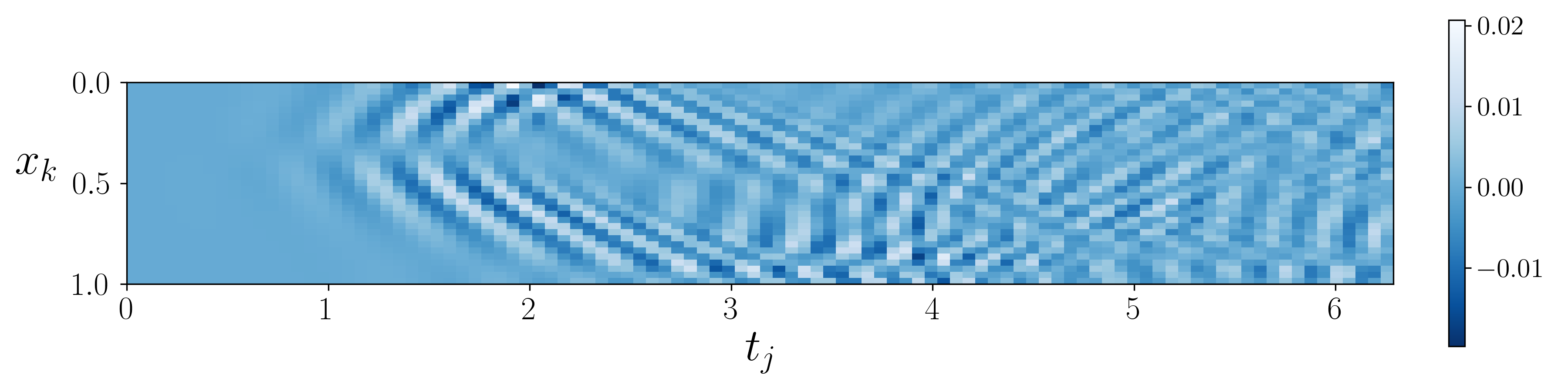
Figure 3: The figure is a plot of the sampled data in $\mathcal{M}$. The pixel $\mathcal{M}(k,j)$ is the measurement value at position $x_{k}$ and time $t_{j}$.

5.3 Results

Tables 3-5 give the relevant measures of error in the reconstructions $R_{\beta}\eta_{0}$, and in Figure 4 we show the reconstructions $R_{\beta}\eta_{0}$ and the pointwise error. We can see that the quality of the reconstruction, both pointwise and in the $L^{2}$-norm, goes from quite poor to quite good as we increase $\beta$. Moreover, we see that the inequalities in Theorem 5 holds true, but that they are not very sharp. If envisioning doing a real experiment, it is also clear that the lack of any dissipation mechanism in (1) makes the model unrealistic, as there would probably be very few waves bouncing around in a small wave tank after the 10 minute measurement time required for Theorem 5 to hold. However, the relative errors on inversion with $T/2$ (as compared to the values in Table 2) are almost identical to those with $T$, indicating the possibility for improving the bounds on the sampling parameteres.

$\beta$	$\frac{\|\eta_{0}-R_{\beta}\eta_{0}\|_{L^{2}}}{\|\eta_{0}\|_{L^{2}}}$	$\frac{\|P_{\beta}\eta_{0}-R_{\beta}\eta_{0}\|_{L^{2}}}{\|P_{\beta}\eta_{0}\|_{L^{2}}}$	$\frac{\|\eta_{0}-P_{\beta}\eta_{0}\|_{L^{2}}}{\|\eta_{0}\|_{L^{2}}}$
8	0.9329	0.0989	0.9322
16	0.5769	0.0177	0.5767
32	0.111	0.008	0.110

Table 3:

$\beta$	$\|P_{\beta}\eta_{0}-R_{\beta}\eta_{0}\|_{L^{2}}$	$\sqrt{\frac{LW}{2(N_{t}-1/\delta)N_{x}}}\|\mathcal{M}_{\beta}-\mathcal{M}\|_{F}$
8	0.00014	0.0227
16	0.00005	0.0270
32	0.000033	0.0107

Table 4:

$\beta$	$\|\eta_{0}-R_{\beta}\eta_{0}\|_{L^{2}}$	$\frac{\sqrt{2}}{\beta}\|\eta_{0}\|_{\dot{H}^{1}}+\sqrt{\frac{LW}{2(N_{t}-1/\delta)N_{x}}}\|\mathcal{M}_{\beta}-\mathcal{M}\|_{F}$
8	0.0037	0.0709
16	0.0023	0.0433
32	0.0005	0.0218

Table 5:

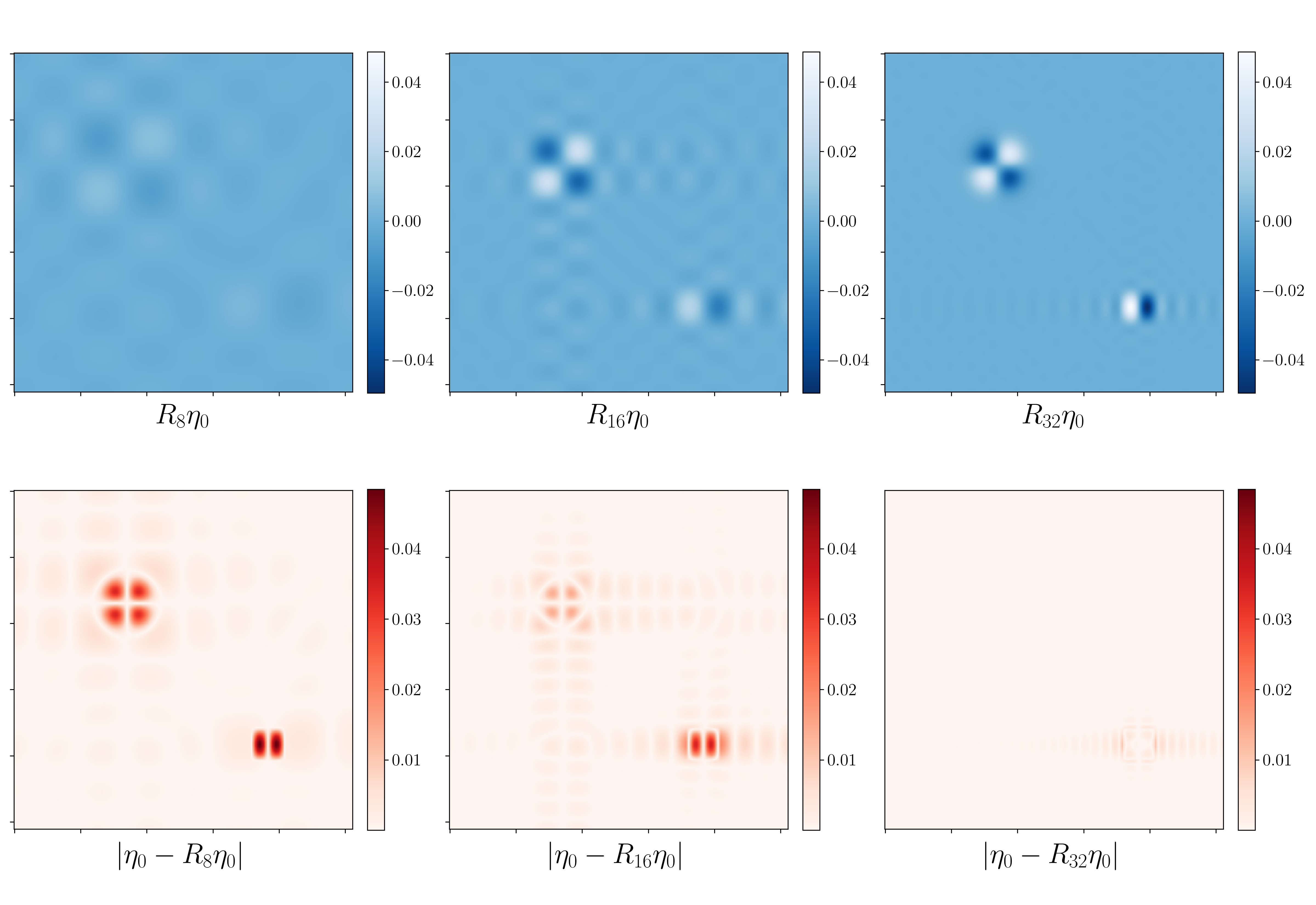
Figure 4: Plot of the reconstruction $R_{\beta}\eta_{0}$ and pointwise error $|R_{\beta}\eta_{0}-\eta_{0}|$ for various $\beta$. The results are in line with the estimates in Theorem 5, and the quality of the reconstruction increases substantially with each doubling of $\beta$

6 Conclusion

We have conducted a rather complete analysis of the linear version of Feynman’s inverse problem. The main finding is the unique continuation property in Section 4.1. We have also shown that one can obtain stability results similar to those known for acoustic and electromagnetic waves for water waves, and that the presence of surface tension is necessary for this to be the case. Moreover, we have proposed and numerically tested a simple reconstruction method applicable to real measurements.

As far as we know, these results are new, and it is tempting to speculate if some the ideas can be applied to other problems; indeed, it seems plausible that it will work for non-linear water wave models like the Stokes wave equation, and we plan pursue this question further. Moreover, it might be that one can rewrite other classical $d$-dimensional PDE as a coupled systems alá (3), and obtain new insights. It would be interesting to consider the inverse problem using one of the (many) non-linear models for water waves, or a compressible fluid model, or the problem where one has a free surface between two non-mixing fluids.

It remains to see if there are any real world applications of the theory, and the author is very open to any suggestions.

We end by going back to the BBC recording. Feynman continues by saying:

And that’s what we’re doing when we’re looking at something. The light that comes out is waves, just like in the swimming pool, except in three dimensions instead of the two dimensions of the pool […] And we have an eight of an inch black hole, into which these things go […] It’s quite wonderful that we figure out so easy… that’s really because the light waves are easier than the waves in the water, [they are] a little bit more complicated. It would have been harder for the bug than for us, but it’s the same idea: to figure out what we are looking at at a distance.

We can reasonably say, at least for waves in a truly incompressible fluid in the linear regime, that Feynman was not entirely correct in his argument. It might be harder for the insect to figure out what is happening in the pool, but it is actually possible, in contrast to what would have been the case if it where observing electromagnetic waves like the eye does.

References

- [1] Mark J Ablowitz. Nonlinear dispersive waves: asymptotic analysis and solitons, volume 47. Cambridge University Press, 2011.
- [2] Vilhelm Adolfsson, Luis Escauriaza, and Carlos E Kenig. Convex domains and unique continuation at the boundary. Revista Matemática Iberoamericana, 11(3):513–525, 1995.
- [3] Thomas Alazard, Pietro Baldi, and Daniel Han-Kwan. Control of water waves. Journal of the European Mathematical Society, 20(3):657–745, 2018.
- [4] Giovanni S Alberti and Yves Capdeboscq. Lectures on elliptic methods for hybrid inverse problems, volume 25. Société Mathématique de France, Paris, 2018.
- [5] Céline Aubel and Helmut Bölcskei. Vandermonde matrices with nodes in the unit disk and the large sieve. Applied and Computational Harmonic Analysis, 47(1):53–86, 2019.
- [6] Yogesh J Bagul, Ramkrishna M Dhaigude, Christophe Chesneau, and Marko Kostić. Tight exponential bounds for hyperbolic tangent. 2021.
- [7] Claude Bardos, Gilles Lebeau, and Jeffrey Rauch. Sharp sufficient conditions for the observation, control, and stabilization of waves from the boundary. SIAM journal on control and optimization, 30(5):1024–1065, 1992.
- [8] Thomas J Bridges, Mark D Groves, and David P Nicholls. Lectures on the theory of water waves, volume 426. Cambridge University Press, 2016.
- [9] Giovanni Covi, Maarten de Hoop, and Mikko Salo. Uniqueness in an inverse problem of fractional elasticity. Proceedings of the Royal Society A, 479(2278):20230474, 2023.
- [10] Walter Craig. Surface water waves and tsunamis. Journal of Dynamics and Differential Equations, 18:525–549, 2006.
- [11] Walter Craig. A course on partial differential equations, volume 197. American Mathematical Soc., 2018.
- [12] A Elcrat, Victor Isakov, Everett Kropf, and D Stewart. A stability analysis of the harmonic continuation. Inverse Problems, 28(7):075016, 2012.
- [13] Marco A Fontelos, Rodrigo Lecaros, JC López, and Jaime H Ortega. Bottom detection through surface measurements on water waves. SIAM Journal on control and optimization, 55(6):3890–3907, 2017.
- [14] Robin Stanley Johnson. A modern introduction to the mathematical theory of water waves. Number 19. Cambridge university press, 1997.
- [15] Barbara Kaltenbacher and William Rundell. Inverse Problems for Fractional Partial Differential Equations, volume 230. American Mathematical Society, 2023.
- [16] Vilmos Komornik and Bernadette Miara. Cross-like internal observability of rectangular membranes. Evolution Equations & Control Theory, 3(1), 2014.
- [17] Nikolai Germanovich Kuznetsov, Vladimir Maz’ya, and Boris Vainberg. Linear water waves: a mathematical approach. Cambridge University Press, 2002.
- [18] David Lannes. The water waves problem: mathematical analysis and asymptotics. American Mathematical Society, 2013.
- [19] Paola Loreti and Vanda Valente. Partial exact controllability for spherical membranes. SIAM journal on control and optimization, 35(2):641–653, 1997.
- [20] Michel Mehrenberger. An ingham type proof for the boundary observability of a n- d wave equation. Comptes Rendus Mathematique, 347(1-2):63–68, 2009.
- [21] Jennifer L Mueller and Samuli Siltanen. Linear and nonlinear inverse problems with practical applications. SIAM, 2012.
- [22] Gerlind Plonka, Daniel Potts, Gabriele Steidl, and Manfred Tasche. Numerical fourier analysis. Springer, 2018.
- [23] Russell M Reid. Control time for gravity-capillary waves on water. SIAM journal on control and optimization, 33(5):1577–1586, 1995.
- [24] Russell M Reid and David L Russell. Boundary control and stability of linear water waves. SIAM journal on control and optimization, 23(1):111–121, 1985.
- [25] Angkana Rüland and Mikko Salo. The fractional calderón problem: low regularity and stability. Nonlinear Analysis, 193:111529, 2020.
- [26] Sandro Salsa. Partial differential equations in action: from modelling to theory, volume 99. Springer, 2016.
- [27] Otmar Scherzer. Handbook of mathematical methods in imaging. Springer Science & Business Media, 2010.
- [28] Mathieu Sellier. Inverse problems in free surface flows: a review. Acta Mechanica, 227(3):913–935, 2016.
- [29] Benjamin K Smeltzer, Eirik Æsøy, Anna Ådnøy, and Simen Å Ellingsen. An improved method for determining near-surface currents from wave dispersion measurements. Journal of Geophysical Research: Oceans, 124(12):8832–8851, 2019.
- [30] Plamen Stefanov. Conditionally stable unique continuation and applications to thermoacoustic tomography. Mathematics in Engineering, 1(4):789–799, 2019.
- [31] Gilbert Strang. The discrete cosine transform. SIAM review, 41(1):135–147, 1999.
- [32] Gerald Tenenbaum and Marius Tucsnak. Fast and strongly localized observation for the schrödinger equation. Transactions of the American Mathematical Society, 361(2):951–977, 2009.
- [33] Marius Tucsnak and George Weiss. Observation and control for operator semigroups. Springer Science & Business Media, 2009.
- [34] Vishal Vasan and Bernard Deconinck. The inverse water wave problem of bathymetry detection. Journal of Fluid Mechanics, 714:562–590, 2013.
- [35] Robert M Young. An introduction to non-Harmonic fourier series, revised edition, 93. Elsevier, 2001.